A General Framework for Mixed Graphical Models

Abstract

“Mixed Data” comprising a large number of heterogeneous variables (e.g. count, binary, continuous, skewed continuous, among other data types) are prevalent in varied areas such as genomics and proteomics, imaging genetics, national security, social networking, and Internet advertising. There have been limited efforts at statistically modeling such mixed data jointly, in part because of the lack of computationally amenable multivariate distributions that can capture direct dependencies between such mixed variables of different types. In this paper, we address this by introducing a novel class of Block Directed Markov Random Fields (BDMRFs). Using the basic building block of node-conditional univariate exponential families from Yang et al. (2012), we introduce a class of mixed conditional random field distributions, that are then chained according to a block-directed acyclic graph to form our class of Block Directed Markov Random Fields (BDMRFs). The Markov independence graph structure underlying a BDMRF thus has both directed and undirected edges. We introduce conditions under which these distributions exist and are normalizable, study several instances of our models, and propose scalable penalized conditional likelihood estimators with statistical guarantees for recovering the underlying network structure. Simulations as well as an application to learning mixed genomic networks from next generation sequencing expression data and mutation data demonstrate the versatility of our methods.

1 Introduction

1.1 Motivation

Acquiring and storing data is steadily becoming cheaper in this Big Data era. A natural consequence of this is more varied and complex data sets, that consist of variables of mixed types; we refer to mixed types as variables measured on the same set of samples that can each belong to differing domains such as binary, categorical, ordinal, counts, continuous, and/or skewed continuous, among others. Consider, for instance, three popular Big Data applications, all of which are comprised of such mixed data:

• High-throughput biomedical data. With new biomedical technologies, scientists can now measure full genomic, proteomic, and metabolomic scans as well as biomedical imaging on a single subject or biological sample.

• National security data. Technologies exist to collect varied information such as call-logs, geographic coordinates, text messages, tweets, demographics, purchasing history, and Internet browsing history, among others.

• Internet-scale marketing data. Internet companies in an effort to optimize advertising revenues collect information such as Internet browsing history, social media postings, friends in social networks, status updates, tweets, purchasing history, ad-click history, and online video viewing history, among others.

In each of these examples, variables of many different types are collected on the same samples, and these variables are clearly dependent. Consider the motivating example of high-throughput “omics” data in further detail. There has been a recent proliferation of genomics technologies that can measure nearly every molecular aspect of a given sample. These technologies, however, produce mixed types of variables: mutations and aberrations such as SNPs and copy number variations are binary or categorical, functional genomics comprising gene expression and miRNA expression as measured by RNA-sequencing are count-valued, and epigenetics as measured by methylation arrays are continuous. Clearly, all of these genomic biomarkers are closely inter-related as they belong to the same complex biological system. Multivariate distributions such as graphical models applied to one type of data, typically gene expression, are popularly used, for tasks ranging from data visualization, finding important biomarkers, and estimating regulatory relationships. Yet, to understand the complete molecular basis of diseases, requires us to understand relationships not only within a specific type of biomarkers, but also between different types of biomarkers. Thus, developing a class of multivariate distributions that can directly model dependencies between genes based on gene expression levels (counts) as well as the mutations (binary) that influence gene expression levels is needed, to holistically model the genomic system. Few such multivariate distributions exist, however, that can directly model dependencies between mixed types of variables. In this paper, our goal is to address this lacuna, and define a parametric family of multivariate distributions, that can model rich dependence structures over mixed variables. We leverage theory of exponential family distributions to do so, and term our resulting novel class of statistical models as mixed Block Directed Markov Random Fields (BDMRFs).

A popular class of statistical studies of such mixed, multivariate data sidestep multivariate densities altogether. Instead, they relate a set of multivariate response variables of one type to multivariate covariate variables of another type, using multiple regression models or multi-task learning models [2]. These are especially popular in expression quantitative trait loci (eQTL) analyses, which seek to link changes in functional gene expression levels to specific genomic mutations [22]. Recent approaches [51] further allow these multiple regression models to associate covariates with mixed types of responses. More general regression and predictive models such as Classification and Regression Trees have also been proposed for such mixed types of covariates [17]. Other approaches implicitly account for variables of mixed types in many machine learning procedures using suitable distance or entropy-based measures [17, 18]. There have also been non-parametric extensions of probabilistic graphical models using copulas [13, 33] or rank-based estimators [45, 31], which could potentially be used for mixed data; non-parametric methods, however, may suffer from a loss of statistical efficiency when compared to parametric families, especially under very high-dimensional sampling regimes. Others have proposed to build network models based on random forests [14] which are able to handle mixed types of variables, but these do not correspond to a multivariate density.

Among parametric statistical modeling approaches for such mixed data, the most popular, especially in survey statistics and spatial statistics [12], are hierarchical models that permit dependencies through latent variables. For example, Sammel et al. [37] propose a latent variable model for mixed continuous and count variables, while Rue et al. [36] propose latent Gaussian models that permit dependencies through a latent Gaussian MRF. While these methods provide statistical models for mixed data, they model dependencies between observed variables via a latent layer that is not observed; estimating these models with strong statistical guarantees is thus typically computationally expensive and possibly intractable.

In this paper, we seek to specify parametric multivariate distributions over mixed types of variables, that directly model dependencies among these variables, without recourse to latent variables, and that are computationally tractable with statistical guarantees for high-dimensional data. Due in part to its importance, there has been some recent set of proposals towards such direct parametric statistical models, building on some seminal earlier work by Lauritzen and Wermuth [26]. We review these in the next sub-section after first providing some background on Markov Random Fields (MRFs). As we will show in the next sub-section, these are however largely targeted to the case where there are variables of two types: discrete and continuous. Some other recent proposals, including some of our prior work, consider more general mixed multivariate distributions, but as we will show these are not sufficiently expressive to allow for rich dependencies between disparate data types. Our proposed class of Block Directed Markov Random Fields (BDMRFs) serve as a vast generalization of these proposals, and indeed as the teleological porting of the work by Lauritzen and Wermuth [26] to the completely heterogeneous mixed data setting.

1.2 Background and Related Work

1.2.1 Markov Random Fields

Suppose $X=(X_{1},\ldots,X_{p})$ is a random vector, with each variable $X_{i}$ taking values in a set $\mathcal{X}$. Let $G_{X}=(V_{X},E_{X})$ be an undirected graph over $p$ nodes corresponding to the $p$ variables $\{X_{s}\}_{s=1}^{p}$. The graphical model over $X$ corresponding to $G_{X}$ is a set of distributions that satisfy Markov independence assumptions with respect to the graph $G_{X}$ [25]. By the Hammersley-Clifford theorem [11], any such distribution that is strictly positive over its domain also factors according to the graph in the following way. Let $\mathcal{C}_{X}$ be a set of cliques (fully-connected subgraphs) of the graph $G_{X}$, and let $\{\phi_{c}(X_{c})\}_{c\in\mathcal{C}_{X}}$ be a set of clique-wise sufficient statistics. Then, any strictly positive distribution of $X$ within the graphical model family represented by the graph $G_{X}$ takes the form:

$$\mathbb{P}[X] \propto \exp\biggr{\{}\sum_{c\in\mathcal{C}_{X}}\theta_{c}\phi_{c}(X_{c})\biggr{\}},$$ (1)

where $\{\theta_{c}\}$ are weights over the sufficient statistics. Popular instances of this model include Ising models [44] for discrete-valued qualitative variables, and Gaussian MRFs [40] for continuous-valued quantitative variables. Ising models specify joint distributions over a set of binary variables each with domain $\mathcal{X}=\{0,1\}$, with the form

$$\mathbb{P}[X]\propto\exp\bigg{\{}\sum_{(s,t)\in E_{X}}\theta_{st}\,X_{s}\,X_{t}\bigg{\}},$$

where we have ignored singleton terms for simplicity. Gaussian MRFs on the other hand specify joint distributions over a set of continuous real-valued variables each with domain $\mathcal{X}=\mathbb{R}$, with the form

$$\mathbb{P}[X]\propto\exp\Bigg{\{}\sum_{s\in V_{X}}\frac{\theta_{s}}{\sigma_{s}}X_{s}+\sum_{(s,t)\in E_{X}}\frac{\theta_{st}}{\sigma_{s}\sigma_{t}}\,X_{s}\,X_{t}-\sum_{s\in V_{X}}\frac{X_{s}^{2}}{2\sigma_{s}^{2}}\Bigg{\}}.$$ (2)

1.2.2 Conditional Gaussian Models

We now review conditional Gaussian models, which were the first proposed class of mixed graphical models, introduced in [26], and further studied in [16, 24, 27, 25]. Let $Y:=(Y_{1},\ldots,Y_{p})\in\mathbb{R}^{p}$ be a continuous response random vector, and let $X:=(X_{1},\ldots,X_{q})\in\{1,\ldots,k\}^{q}$ be a discrete covariate random vector. Taken together, $(X,Y)$ is then a mixed random vector with both continuous and discrete components. For such a mixed random vector, [26] proposed the following joint distribution:

$$\mathbb{P}[X,Y]=\exp\left\{g(X)+h(X)^{T}Y-\frac{Y^{T}K(X)Y}{2}\right\},$$ (3)

parameterized by $g(X)\in\mathbb{R}$, $h(X)\in\mathbb{R}^{p}$, and $K(X)\in\mathbb{R}^{p\times p}$, such that $K(X)\succeq 0$. They termed this model a conditional Gaussian (CG) model, since the conditional distribution of $\mathbb{P}[Y|X]$ given the joint distribution in (3) is given by a multivariate Gaussian distribution:

$$\mathbb{P}[Y|X]\equiv\mathcal{N}(K(X)^{-1}h(X),\,K(X)^{-1}).$$

Consider the set of vertices $V_{X}$ and $V_{Y}$ corresponding to random variables in $X$ and $Y$ respectively, and consider the set joint vertices $V=V_{X}\cup V_{Y}$. Would Markov assumptions with respect to a graph $G=(V,E)$ over all the vertices entail restrictions on $g(X),h(X),K(X)$ in the joint distribution in (3)? In the following theorem from Lauritzen and Wermuth [26], which we reproduce for completeness, they provide an answer to this question:

Theorem 1.

If the CG distribution in (3) is Markov with respect to a graph $G$, then $g(X),h(X),K(X)$ can be written as

$$g(X)=\sum_{d\subseteq[q]}g_{d}(X),\ h(X)=\sum_{d\subseteq[q]}h_{d}(X),\ K(X)=\sum_{d\subseteq[q]}K_{d}(X),$$

where we use $[q]$ to denote $\{1,\ldots,q\}$ and

• $g_{d}(X),h_{d}(X),K_{d}(X)$ depend on $X$ only through the subvector $X_{d}$,

• for any subset $d\subseteq[q]$ which is not complete with respect to $G$, the corresponding components are zero, so that $g_{d}(X)=0,h_{d}(X)=0,K_{d}(X)=0$.

Recently, there have been several proposals for estimating the graph structure of these CG models in high-dimensional settings. Lee and Hastie [28] consider a specialization of CG models involving only pairwise interactions between any two variables and propose sparse node-wise estimators for graph selection. Cheng et al. [8] further consider three-way interactions between two binary variables and one continuous variable and also propose sparse node-wise estimators to select the network structure.

1.2.3 Graphical Models beyond Ising and Gaussian MRFs, via Exponential Families

A key caveat with the CG models as defined in (3) and [26], however, is that it is specifically constructed for mixed discrete and thin-tailed continuous data. What if the responses and/or the covariates were count-valued, or skewed-continuous, or belonged to some other non-categorical non-thin-tailed-continuous data type? This is the question we address in this paper. Towards this, we first briefly review here a recent line of work [46, 48, 50] (which extends earlier work by Besag [5]) which specified undirected graphical model distributions where the variables all belong to one data-type, but which could be any among a wide class of data-types. Their development was as follows. Consider the general class of univariate exponential family distributions (which include many popular distributions such as Bernoulli, Gaussian, Poisson, negative binomial, and exponential, among others):

$$\mathbb{P}[Z;\theta]=\exp\Big{\{}\theta\,B(Z)+M(Z)-D(\theta)\Big{\}},$$ (4)

with sufficient statistics $B(Z)$, base measure $M(Z)$, and log-normalization constant $D(\theta)$. Suppose that $p$-dimensional random vector $X$ has node-conditional distributions specified by an exponential family,

$$\log\mathbb{P}[X_{s}|X_{V_{X}\backslash s}]=E(X_{V_{X}\backslash s})\,B(X_{s})+M(X_{s})-\bar{D}(X_{V_{X}\backslash s}),$$

where the function $E(X_{V_{X}\backslash s})$ is any function that depends on the rest of all random variables except $X_{s}$. Further suppose that the corresponding joint distribution $\mathbb{P}_{\exp}[X]$ factors according to the set of cliques $\mathcal{C}_{X}$ of a graph $G_{X}$. Yang et al. [46] then showed that such a joint distribution consistent with the above node-conditional distributions exists, and moreover necessarily has the form

$$\log\mathbb{P}_{\exp}[X]=\sum_{C\in\mathcal{C}_{X}}\theta_{C}\prod_{s\in C}B(X_{s})+\sum_{s\in V_{X}}M(X_{s})-A(\theta)$$ (5)

where the function $A(\theta)$ is so-called log-partition function, that provides the log-normalization constant for the multivariate distribution.

Yang et al. [48] then developed the conditional extension of (5) above. Consider a response random vector $Y:=(Y_{1},\ldots,Y_{p})\in\mathcal{Y}^{p}$ and a covariate random vector $X:=(X_{1},\ldots,X_{q})\in\mathcal{X}^{q}$. Suppose that the node conditional distributions of $Y_{s}$ for all $s\in V_{Y}$ follow exponential families:

$$\log\mathbb{P}[Y_{s}|Y_{V_{Y}\backslash s},X]=E(Y_{V_{Y}\backslash s},X)\,B(Y_{s})+M(Y_{s})-\bar{D}(Y_{V_{Y}\backslash s},X),$$

and that the corresponding joint $\mathbb{P}_{\exp}[Y|X]$ factors according to set of cliques $\mathcal{C}_{Y}$ among random variables in $Y$. Then, [48] showed that such a joint distribution consistent with the node-conditional distributions does exist, and necessarily has the form:

$$\log\mathbb{P}_{\exp}[Y|X]=\sum_{C\in\mathcal{C}_{Y}}\theta_{C}(X)\prod_{s\in C}B(Y_{s})+\sum_{s\in V_{Y}}M(Y_{s})-A_{Y|X}\big{(}\theta(X)\big{)},$$ (6)

where $\theta_{C}(X)$ is any function that only depends on the random vector $X$.

1.2.4 Mixed MRFs

While (5),(6) specify multivariate distributions for variables of varied data-types, they are nonetheless specified for the setting where all the variables belong to the same type. Accordingly, there have been some recent extensions [50, 7] of the above for the more general setting of interest in this paper, where each variable belongs to a potentially different type. Their construction was as follows, and can be seen to be an extension not only of the class of exponential family MRFs in (5), but also of the class of conditional Gaussian models in (3). Suppose that the node conditional distributions of each variable $X_{s}$ for $s\in V_{X}$ now belongs to potentially differing univariate exponential families:

$$\log\mathbb{P}[X_{s}|X_{V_{X}\backslash s}]=E_{s}(X_{V_{X}\backslash s})\,B_{s}(X_{s})+M_{s}(X_{s})-\bar{D}_{s}(X_{V_{X}\backslash s}),$$

while as before, we require the corresponding joint distribution $\mathbb{P}_{\exp}[X]$ to factor according to the set of cliques $\mathcal{C}_{X}$ of a graph $G_{X}$. In a precursor to this paper Yang et al. [50], we showed that such a joint distribution consistent with the node-conditional distributions does exist, and moreover necessarily has the form

$$\log\mathbb{P}_{\exp}[X]=\sum_{C\in\mathcal{C}_{X}}\theta_{C}\prod_{s\in C}B_{s}(X_{s})+\sum_{s\in V_{X}}M_{s}(X_{s})-A(\theta)$$ (7)

where the sufficient statistics $B_{s}(\cdot)$ and base measure $M_{s}(\cdot)$ in this case can be different across random variables. While these provide multivariate distributions over heterogeneous variables, as we will show in the main section of the paper, this class of distributions sometimes have stringent normalizability restrictions on the set of parameters $\{\theta_{C}\}$. In this paper, we thus develop a far more extensive generalization that leverages block-directed graphs.

1.3 Summary & Organization

This paper is organized as follows. In Section 2, we first introduce the class of Elementary Block Directed Markov Random Fields (EBDMRFs), which are the simplest subclass of our class of graphical models. Here, we assume the heterogeneous set of variables can be grouped into two groups: $X$ and $Y$ (each of which could have heterogeneous variables in turn). Our class of EBDMRFs are then specified via a simple application of the chain rule as $\mathbb{P}[X,Y]=\mathbb{P}_{\exp}[Y|X]\,\mathbb{P}_{\exp}[X]$, where $\mathbb{P}_{\exp}[X]$ is set to an exponential family mixed MRF as in (7) from [50], and $\mathbb{P}_{\exp}[Y|X]$ is a novel class of what we call exponential family mixed CRFs, that extend our prior work on exponential family CRFs in (6) from [48], and exponential family mixed MRFs in (7) from [50]. This can be seen as a generalization of the seminal mixed graphical models work of [26]. We then discuss the properties of this class of distribution, including conditions or restrictions on the parameter space under which the distribution is normalizability. As we show, our formulation of EBDMRFs have substantially weaker normalizability restrictions when compared with our preliminary work on exponential family mixed MRFs [50].

In Section 3, we then extend this construction further by recursively applying the chain rule respecting a directed acyclic graph over blocks of variables, resulting in a class of graphical models we call Block Directed Markov Random Fields (BDMRFs). The overall underlying graph of this class of graphical models thus has both directed edges between blocks of variables and undirected edges within blocks of variables. Our construction yields a very general and flexible class of mixed graphical models that directly parameterizes dependencies over mixed variables. We study the problem of parameter estimation and graph structure learning for our class of BDMRF models in Section 4, providing statistical guarantees on the recovery of our models even under high-dimensional regimes. Finally, in Section 5 and Section 6, we demonstrate the flexibility and applicability of our models via both an empirical study of our estimators through a series of simulations, as well as an application to high-throughput cancer genomics data.

2 Elementary Block Directed Markov Random Fields (EBDMRFs)

In this section, we will introduce a simpler subclass of our eventual class of graphical models which we term Elementary Block Directed Markov Random Fields (EBDMRFs). Before doing so, we first develop a key building block: a novel class of conditional distributions.

2.1 Exponential Family Mixed CRFs

We now consider the modeling of the conditional distribution of a heterogeneous random response vector $Y:=(Y_{1},\ldots,Y_{p})\in\mathcal{Y}_{1}\times\ldots\times\mathcal{Y}_{p}$, conditioned on a heterogeneous random covariate vector $X:=(X_{1},\ldots,X_{q})\in\mathcal{X}_{1}\times\ldots\times\mathcal{X}_{q}$. Suppose that we have a graph $G_{Y}=(V_{Y},E_{Y})$, with nodes $V_{Y}$ associated with variables in $Y$. Denote the set of cliques of this graph by $C_{Y}$, and the set of response neighbors in $V_{Y}$ for any response node $s\in V_{Y}$ by $N_{Y}(s)$. Suppose further that we also have a set of nodes $V_{X}$ associated with the covariate variables in $X$, and that for any response node $s\in V_{Y}$, we have a set of covariate neighbors in $V_{X}$ denoted by $N_{YX}(s)$.

Suppose that the response variables $Y$ are locally Markov with respect to their specified neighbors, so that

$$\mathbb{P}[Y_{s}|Y_{V_{Y}\backslash s},X]=\mathbb{P}[Y_{s}|Y_{N_{Y}(s)},X_{N_{YX}(s)}].$$ (8)

Moreover, suppose that this conditional distribution $Y_{s}$ conditioned on the rest of $Y_{V_{Y}\backslash s}$ and $X$ is given by an arbitrary univariate exponential family:

$$\log\mathbb{P}[Y_{s}|Y_{V_{Y}\backslash s},X]=E_{s}\big{(}Y_{V_{Y}\backslash s},X\big{)}\,B_{s}(Y_{s})+M_{s}(Y_{s})-\bar{D}_{s}\big{(}Y_{V_{Y}\backslash s},X\big{)},$$ (9)

with sufficient statistic $B_{s}(\cdot)$ and base measure $M_{s}(\cdot)$. Note that there is no assumption on the form of functions $E_{s}\big{(}Y_{V_{Y}\backslash s},X\big{)}$. The following theorem then specifies the algebraic form of the conditional distribution $\mathbb{P}_{\exp}[Y|X]$.

Theorem 2.

Consider a $p$-dimensional random vector $Y=(Y_{1},\ldots,Y_{p})$ denoting the set of responses, and let $X=(X_{1},\ldots,X_{q})$ be a $q$-dimensional covariate vector. Then, the node-wise conditional distributions satisfying the Markov condition in (8) as well as the exponential family condition in (9), are indeed consistent with a graphical model joint distribution, that factors according to $G_{Y}$, and has the form:

$$\log\mathbb{P}_{\exp}[Y|X]=\sum_{C\in\mathcal{C}_{Y}}\theta_{C}\big{(}X_{N_{YX}(C)}\big{)}\prod_{s\in C}B_{s}(Y_{s})+\sum_{s\in V_{Y}}M_{s}(Y_{s})-A_{Y|X}\big{(}\theta(X)\big{)},$$ (10)

where $N_{YX}(C)={\cap_{s\in C}}N_{YX}(s)$ and $A_{Y|X}\big{(}\theta(X)\big{)}$ is the log-normalization function, which is the function on the set of parameters $\{\theta_{C}\big{(}X_{N_{YX}(C)}\big{)}\}_{C\in\mathcal{C}_{Y}}$.

The proof of the theorem follows along similar lines to that of the Hammersley Clifford Theorem, and is detailed in Appendix 8.1. In Appendix 8.5, we also discuss constraints on the covariate parameter functions $\{\theta_{C}(\cdot)\}_{C\in\mathcal{C}_{Y}}$ that ensure the distribution is normalizable. Note that to ensure the Global Markov Property holds, these can be arbitrarily specified as long as they are functions solely of the covariate neighborhoods.

We term this class of conditional distributions as exponential family mixed CRFs. Notice that this framework provides a multivariate density over the random response vector $Y$, but not a joint density over both $X$ and $Y$ as we ultimately desire.

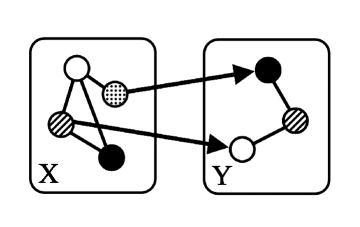
Figure 1: Elementary Block Directed MRF

2.2 Model Specification: EBDMRFs

We assume that the heterogeneous set of variables can be partitioned into two groups $X:=(X_{1},\ldots,X_{q})\in\mathcal{X}_{1}\otimes\ldots\mathcal{X}_{q}$ and $Y:=(Y_{1},\ldots,Y_{p})\in\mathcal{Y}_{1}\otimes\ldots\mathcal{Y}_{p}$; note that each group could in turn be heterogeneous. Such a delineation of the overall set of variables into two groups is natural in many settings. For instance, the variables in $X$ could be the set of covariates, while the variables in $Y$ could be the set of responses, or $X$ could be cause variables, while $Y$ could be effect variables, and so on. Given the ordering of variables $(X,Y)$, suppose it is of interest to specify dependencies among $Y$ conditioned on $X$, and then of the marginal dependencies among $X$.

Towards this, suppose that we have an undirected graph $G_{Y}=(V_{Y},E_{Y})$, with nodes $V_{Y}$ associated with variables in $Y$, and set of cliques $C_{Y}$, and in addition, an undirected graph $G_{X}=(V_{X},E_{X})$, with nodes $V_{X}$ associated with variables in $X$, and set of cliques $C_{X}$. Suppose in addition, we have directed edges $E_{XY}$ from nodes in $V_{X}$ to $V_{Y}$. Thus, the overall graph structure has both undirected edges $E_{X}$ and $E_{Y}$ among nodes solely in $X$ and $Y$ respectively, as well as directed edges $E_{XY}$, from nodes in $X$ to $Y$, as shown in Fig. 1. For any response node $s\in V_{Y}$, we will denote the set of response-specific neighbors in $G_{Y}$ by $N_{Y}(s)$, and we will again denote covariate-specific neighbors in $V_{X}$, by $N_{YX}(s)$.

Armed with this notation, we propose the following natural joint distribution over $(X,Y)$:

$$\mathbb{P}[X,Y]=\mathbb{P}_{\exp}[Y|X]\,\mathbb{P}_{\exp}[X],$$

where the two pieces, $\mathbb{P}_{\exp}[Y|X]$ and $\mathbb{P}_{\exp}[X]$, are specified as follows. The conditional distribution $\mathbb{P}_{\exp}[Y|X]$ is specified by an exponential family mixed CRF as in (10),

$$\log\mathbb{P}_{\exp}[Y|X]=\sum_{C\in\mathcal{C}_{Y}}\theta_{C}\big{(}X_{N_{YX}(C)}\big{)}\prod_{s\in C}B_{s}(Y_{s})+\sum_{s\in V_{Y}}M_{s}(Y_{s})-A_{Y|X}\big{(}\theta(X)\big{)},$$

while the marginal distribution $\mathbb{P}_{\exp}[X]$ is specified by an exponential family mixed MRF as in (7),

$$\log\mathbb{P}_{\exp}[X]=\sum_{C\in\mathcal{C}_{X}}\theta_{C}\prod_{t\in C}B_{t}(X_{t})+\sum_{t\in V_{X}}M_{t}(X_{t})-A_{X}(\theta).$$

Thus, the overall joint distribution, which we call an Elementary Block Directed Markov Random Field (EBDMRF) is given as:

$$\log\mathbb{P}[X,Y] =\sum_{C\in\mathcal{C}_{Y}}\theta_{C}\big{(}X_{N_{YX}(C)}\big{)}\prod_{s\in C}B_{s}(Y_{s})+\sum_{s\in V_{Y}}M_{s}(Y_{s})+\sum_{C\in\mathcal{C}_{X}}\theta_{C}\prod_{t\in C}B_{t}(X_{t})$$

$$\qquad+\sum_{t\in V_{X}}M_{t}(X_{t})-A_{Y|X}\big{(}\theta(X)\big{)}-A_{X}(\theta).$$ (11)

We provide additional intuition on our class of EBDMRF distributions in the next few sections. First, we compare the conditional independence assumptions entailed by the mixed graph of the EBDMRF with the Global Markov assumptions entailed by an undirected graph in Section 2.3. Then in Section 2.4, we compare the form of the EBDMRF class of distributions with that of the mixed MRF distributions introduced earlier in Section 1.2.4. Next, we analyze the domain of the parameters of the distribution by considering parameter restrictions to ensure normalizability in Section 2.5. Finally, in Section 2.6, we provide several examples of our EBDMRF distributions, compare these to Mixed MRF distribution counterparts, and place them in the context of the larger graphical models literature.

2.3 Global Markov Structure

The EBDMRF distribution is specified by a mixed graph with both directed edges from $V_{X}$ to $V_{Y}$ and undirected edges within $V_{X}$ and $V_{Y}$. A natural question that arises then is what are the conditional independence assumptions specified by the edges in the mixed graph? Consider the undirected edges in $G_{X}$: by construction, these represent the Markov conditional independence assumptions in the marginal distribution $\mathbb{P}_{\exp}[X]$. The remaining undirected and directed edges incident on the response nodes $V_{Y}$ in turn represent Markov assumptions in the conditional distribution $\mathbb{P}_{\exp}[Y|X]$ as described in (8) in the previous section. It can thus be seen that the set of conditional independence assumptions entailed by the mixed graph differ from those of a purely undirected graph obtained from the mixed graph by dropping the orientations of the edges from nodes in $V_{Y}$ to nodes in $V_{X}$.

But under what additional restrictions would a EBDMRF entail Markov independence assumptions with respect to an undirected graph over the joint set of vertices $V=V_{X}\cup V_{Y}$? This was precisely the question asked in the classical mixed graphical model work of [26]. Specifically, we are interested in outlining what restrictions on $\theta(\cdot)$ in the joint distribution in (11) would entail global Markov assumptions with respect to a graph $G=(V,E)$ over all the vertices $V=V_{X}\cup V_{Y}$. In the following theorem, we provide an answer to this question:

Theorem 3.

Consider an EBDMRF distribution of the form (11), with graph structure specified by undirected edges $E_{X}$ among nodes in $V_{X}$, and $E_{Y}$ among nodes in $V_{Y}$, as well as directed edges $E_{XY}$ from nodes in $V_{X}$ to $V_{Y}$. Then, if this distribution is globally Markov with respect to a graph $G=(V,E)$ with nodes $V=V_{X}\cup V_{Y}$ and edges $E\subseteq V\times V$, then

• $E_{X},E_{Y},E_{XY}\subseteq E$.

• For all response cliques $C\in\mathcal{C}_{Y}$,

  $$\theta_{C}(X)=\sum_{d\subseteq N_{YX}(C)}\theta_{C,d}(X),$$

  where $\theta_{C,d}(X)$ depends on $X$ only through the subvector $X_{\{d\}\cup C}$, and that for any subset $d\subseteq[q]$ such that $\{d\}\cup C$ is not complete with respect to $G$, $\theta_{C,d}(X)=0$.

The theorem thus entails that the covariate parameters $\theta$ and $\theta(\cdot)$ in (11) factor with respect to the overall graph $G$. In other words to ensure the Global Markov structure holds, the covariate parameters can be arbitrarily specified as long as they are functions solely of the covariate-neighborhoods.

2.4 Comparison to Mixed MRFs

The previous section investigated the implications as far as global Markov properties for our EBDMRF distribution with both directed and undirected edges as compared to the undirected edges of the mixed MRF distribution. Here, we compare and contrast the factorized form of these distributions, in part because the key reason for the popularity of graphical model distributions is the factored form of their joint distributions.

Suppose we have two sets of variable, $X$ and $Y$, and consider the case of pairwise interactions. Then, this special case of the mixed MRF distributions in Section 1.2.4 can be written as:

$$\log\mathbb{P}_{\exp}[X,Y]= \sum_{s\in V_{Y}}\theta_{s}B_{s}(Y_{s})+\sum_{t\in V_{X}}\theta_{t}B_{t}(X_{t})+\sum_{(s,s^{\prime})\in E_{Y}}\theta_{ss^{\prime}}\,B_{s}(Y_{s})\,B_{s^{\prime}}(Y_{s^{\prime}})$$

$$+\sum_{(t,t^{\prime})\in E_{X}}\theta_{tt^{\prime}}\,B_{t}(X_{t})\,B_{t^{\prime}}(X_{t^{\prime}})+\sum_{(s,t)\in E_{XY}}\theta_{st}\,B_{s}(Y_{s})\,B_{t}(X_{t})$$

$$+\sum_{s\in V_{Y}}M_{s}(Y_{s})+\sum_{t\in V_{X}}M_{t}(X_{t})-A(\theta)$$ (12)

For this same pairwise case, the EBDMRF class of distributions in (11) can be written as:

$$\log\mathbb{P}[X,Y]= \sum_{s\in V_{Y}}\theta_{s}(X_{N_{YX}(s)})B_{s}(Y_{s})+\sum_{(s,s^{\prime})\in E_{Y}}\theta_{ss^{\prime}}(X_{N_{YX}(s,s^{\prime})})\,B_{s}(Y_{s})\,B_{s^{\prime}}(Y_{s^{\prime}})$$

$$+\sum_{t\in V_{X}}\theta_{t}B_{t}(X_{t})+\sum_{(t,t^{\prime})\in E_{X}}\theta_{tt^{\prime}}\,B_{t}(X_{t})\,B_{t^{\prime}}(X_{t^{\prime}})$$

$$+\sum_{s\in V_{Y}}M_{s}(Y_{s})+\sum_{t\in V_{X}}M_{t}(X_{t})-A_{Y|X}\big{(}\theta(X)\big{)}-A_{X}(\theta).$$ (13)

Noting that covariate functions can be set arbitrarily, it can be seen that the two distributions have almost similar forms when we set the covariate functions $\{\theta_{s}(X_{N_{YX}(s)}),\theta_{ss^{\prime}}(X_{N_{YX}(s,s^{\prime})})\}$ as

$$\theta_{s}(X_{N_{YX}(s)}):=\theta_{s}+\sum_{t\in N_{YX}(s)}\theta_{st}\,B_{t}(X_{t}),\quad\text{and}\quad\theta_{ss^{\prime}}(X_{N_{YX}(s,s^{\prime})}):=\theta_{ss^{\prime}}.$$ (14)

In this case, the EBDMRF distribution in (2.4) and the mixed MRF distribution in (2.4) differ primarily due to the non-linear term $A_{Y|X}(\theta(X))$. Notice that in (2.4), $A(\theta)$ is only dependent on parameters and hence the form (2.4) and indeed more generally all mixed MRFs belong to the class of multivariate exponential family distributions. On the other hand, $A_{Y|X}(\theta(X))$ in (2.4) depends on $X$ and hence even when the covariate functions are simple linear forms as in (14), these are not exponential family distributions.

Similarly, the conditional distribution $\mathbb{P}_{\exp}[X|Y]$ of mixed MRF distribution in (2.4) can be easily derived as:

$$\log\mathbb{P}[X|Y]\propto \sum_{t\in V_{X}}\Big{(}\theta_{t}+\sum_{s\,|\,(s,t)\in E_{XY}}\theta_{st}\,B_{s}(Y_{s})\Big{)}B_{t}(X_{t})$$

$$+\sum_{(t,t^{\prime})\in E_{X}}\theta_{tt^{\prime}}\,B_{t}(X_{t})\,B_{t^{\prime}}(X_{t^{\prime}})+\sum_{t\in V_{X}}M_{t}(X_{t}),$$

while the conditional distribution $\mathbb{P}[X|Y]$ for the case of the EBDMRF, when setting the covariate functions $\{\theta_{s}(X_{N_{YX}(s)}),\theta_{ss^{\prime}}(X_{N_{YX}(s,s^{\prime})})\}$ as in (14), can be written as

$$\log\mathbb{P}[X|Y]\propto\sum_{t\in V_{X}}\Big{(}\theta_{t}+\sum_{s\,|\,(s,t)\in E_{XY}}\theta_{st}\,B_{s}(Y_{s})\Big{)}B_{t}(X_{t})$$

$$+\sum_{(t,t^{\prime})\in E_{X}}\theta_{tt^{\prime}}\,B_{t}(X_{t})\,B_{t^{\prime}}(X_{t^{\prime}})+\sum_{t\in V_{X}}M_{t}(X_{t})-A_{Y|X}(\theta(X)),$$

which can again be seen to differ primarily due to the term $A_{Y|X}(\theta(X))$.

It is also instructive to consider the differing forms of the conditional distributions $\mathbb{P}[Y|X]$ in general. For pairwise mixed MRFs, this can be written as

$$\log\mathbb{P}_{\exp}[Y|X] \propto\sum_{s\in V_{Y}}\Big{(}\theta_{s}+\sum_{t\,|\,(s,t)\in E_{XY}}\theta_{st}\,B_{t}(X_{t})\Big{)}B_{s}(Y_{s})$$

$$+\sum_{(s,s^{\prime})\in E_{Y}}\theta_{ss^{\prime}}\,B_{s}(Y_{s})\,B_{s^{\prime}}(Y_{s^{\prime}})+\sum_{s\in V_{Y}}M_{s}(Y_{s}),$$ (15)

while that for the pairwise EBDMRF can be written as

$$\log\mathbb{P}[Y|X] \propto\sum_{s\in V_{Y}}\theta_{s}(X_{N_{YX}(s)})B_{s}(Y_{s})$$

$$+\sum_{(s,s^{\prime})\in E_{Y}}\theta_{ss^{\prime}}(X_{N_{YX}(s,s^{\prime})})\,B_{s}(Y_{s})\,B_{s^{\prime}}(Y_{s^{\prime}})+\sum_{s\in V_{Y}}M_{s}(Y_{s}).$$ (16)

Thus, the two distributions differ only because the covariate functions $\{\theta_{s}(X_{N_{YX}(s)})\}$, $\{\theta_{ss^{\prime}}(X_{N_{YX}(s,s^{\prime})})\}$ in the EBDMRF distribution can be set arbitrarily. However, when they are set precisely equal to the expressions in (14), these two distributions can be seen to identical. Overall, the pairwise EBDMRF and Mixed MRF distributions are strikingly similar in the case where the EBDMRF distribution has linear covariate functions, differing only by the normalization terms $A_{Y|X}(\theta(X))$. This seemingly minor difference, however, has important consequences in terms of normalizability discussed next.

2.5 Normalizability

An important advantage of our EBDMRF class of distributions is that the parameter restrictions for normalizability of (11) can be characterized simply. Recall that the problem of normalizability refers to the set of restrictions on the parameter space that is required to ensure the joint density integrates to one; this entails ensuring that the log-partition functions are finitely integrable.

Theorem 4.

For any given set of parameters, the joint distribution in (11) exists and is well-defined, so long as the corresponding marginal MRF $\mathbb{P}_{\exp}[X]$, as well as the conditional distribution $\mathbb{P}_{\exp}[Y|X]$ are well-defined.

Thus the normalizability conditions for the joint distribution in (11) reduces to those for the marginal MRF $\mathbb{P}_{\exp}[X]$ and for the mixed CRF $\mathbb{P}_{\exp}[Y|X]$.

In the previous section, we saw that the pairwise EBDMRF and the pairwise mixed MRF distributions have very similar form when the covariate functions $\{\theta_{s}(X_{N_{YX}(s)}),\theta_{ss^{\prime}}(X_{N_{YX}(s,s^{\prime})})\}$ are set as in (14). It will thus be instructive to compare the normalizability restrictions imposed on the mixed MRF parameters with those on the EBDMRF parameters in this special case.

Let us introduce shorthand notations for the following expressions:

$$F(X;\theta)=\sum_{t\in V_{X}}\theta_{t}B_{t}(X_{t})+\sum_{(t,t^{\prime})\in E_{X}}\theta_{tt^{\prime}}\,B_{t}(X_{t})\,B_{t^{\prime}}(X_{t^{\prime}})+\sum_{t\in V_{X}}M_{t}(X_{t})\,,$$

$$F(X,Y;\theta)=\sum_{s\in V_{Y}}\theta_{s}B_{s}(Y_{s})+\sum_{(s,s^{\prime})\in E_{Y}}\theta_{ss^{\prime}}\,B_{s}(Y_{s})\,B_{s^{\prime}}(Y_{s^{\prime}})$$

$$+\sum_{(s,t)\in E_{XY}}\theta_{st}\,B_{s}(Y_{s})\,B_{t}(X_{t})+\sum_{s\in V_{Y}}M_{s}(Y_{s}).$$

Then, the log-partition function $A(\theta)$ in the mixed MRF distribution (2.4) can be written as

$$A(\theta) :=\log\left(\sum_{X,Y}\exp\Big{\{}F(X;\theta)+F(X,Y;\theta)\Big{\}}\right)$$

$$=\log\left(\sum_{X}\Big{[}\exp\{F(X;\theta)\}\sum_{Y}\exp\{F(X,Y;\theta)\}\Big{]}\right).$$ (17)

On the other hand, the pairwise EBDMRF distribution in (2.4) has the following two “normalization” terms:

$$A_{Y|X}\big{(}\theta(X)\big{)} :=\log\left(\sum_{Y}\exp\{F(X,Y;\theta)\}\right)\,,$$

$$A_{X}(\theta) :=\log\left(\sum_{X}\exp\{F(X;\theta)\}\right).$$

Thus, the overall “normalization” term in (2.4) can be written as:

$$A_{Y|X}\big{(}\theta(X)\big{)}+A_{X}(\theta)= \log\left(\sum_{Y}\exp\{F(X,Y;\theta)\}\right)+\log\left(\sum_{X}\exp\{F(X;\theta)\}\right)$$

$$= \log\left\{\left(\sum_{X}\exp\{F(X;\theta)\}\right)\left(\sum_{Y}\exp\{F(X,Y;\theta)\}\right)\right\}.$$ (18)

In contrast to those of the mixed MRF, these terms are not normalization constants as the term $A_{Y|X}\big{(}\theta(X)\big{)}$ is a function of $X$. Comparing (2.5) and (2.5), it can be seen that the two expressions become identical in the special case where $\theta_{st}=0$ for all $(s,t)\in E_{XY}$, which would entail that $X$ and $Y$ are independent, and that $F(X,Y;\theta)$ is only a function of $Y$.

But more generally, how would the two different normalization terms affect the normalizability of the two classes of distributions? Would one necessarily be more restrictive than the other? Interestingly, the following theorem indicates that the EBDMRF distribution imposes strictly weaker conditions for normalizability.

Theorem 5.

Consider the pairwise mixed MRF distribution (2.4). Then, if its log-partition function $A(\theta)$ is finite, then the EBDMRF distribution form in (2.4), with the covariate functions $\{\theta_{s}(X_{N_{YX}(s)}),\theta_{ss^{\prime}}(X_{N_{YX}(s,s^{\prime})})\}$ set to the linear forms in (14), is normalizable as well.

We provide a proof of this assertion in Appendix 8.4. Namely if the log-partition function $A(\theta)$ in (2.5) is finite, then both $A_{Y|X}(\theta(X))$ and $A_{X}(\theta)$ in (2.5) must also be finite; thus, if pairwise mixed MRFs are normalizable, then so are EBDMRFs. The inverse of statement in Theorem 5 does not hold in general, which can be demonstrated by several counter-examples discussed in the next section.

2.6 Examples

We provide several examples of EBDMRFs to better illustrate the properties and implications of our models, and relate them to the broader graphical models literature.

Gaussian-Ising EBDMRFs

Gaussian-Ising mixed graphical models have been well studied in the literature [26, 8, 28, 50]. Here, we show that each of these studied classes are a special case of our class of EBDMRF models, and which in addition provide other formulations of these mixed models. Suppose we have a set of binary valued random variables $X$, each with domain $\mathcal{X}\in\{-1,1\}$, and a set of continuous valued random variables $Y$, each with domain, $\mathcal{Y}\in\mathbb{R}$. We can specify the node-conditional distributions associated with $X$ as Bernoulli with sufficient statistics and base measure given by $B_{t}(X_{t})=X_{t}$, $M_{t}(X_{t})=0$ for all $t\in V_{X}$; similarly, we can specify the node-conditionals associated with $Y$ as Gaussian with sufficient statistics and base measure given by $B_{s}(Y_{s})=\frac{Y_{s}}{\sigma_{s}}$, and $M_{s}(Y_{s})=-\frac{Y_{s}^{2}}{2\sigma^{2}_{s}}$, respectively for all $s\in V_{Y}$. Given these two sets of binary and real valued random variables, there are then three primary ways of specifying joint EBDMRF distributions: the mixed MRF $\mathbb{P}_{\exp}[X,Y]$ from Yang et al. [50], Chen et al. [7] , the EBDMRF specified by $\mathbb{P}_{\exp}[Y|X]\,\mathbb{P}_{\exp}[X]$, and the EBDMRF specified by $\mathbb{P}_{\exp}[X|Y]\,\mathbb{P}_{\exp}[Y]$; note that these various formulations do not coincide and give distinct ways of modeling a joint density. When we consider only pairwise interactions and linear covariate functions as in (14), these models all take a similar form, only differing in the log-normalization terms:

$$\log\mathbb{P}[X,Y] =\sum_{s\in V_{Y}}\frac{\theta_{s}}{\sigma_{s}}Y_{s}+\sum_{t\in V_{X}}\theta_{t}X_{t}+\sum_{(s,s^{\prime})\in E_{Y}}\frac{\theta_{ss^{\prime}}}{\sigma_{s}\sigma_{s^{\prime}}}Y_{s}Y_{s^{\prime}}$$

$$+\sum_{(t,t^{\prime})\in E_{X}}\theta_{tt^{\prime}}\,X_{t}\,X_{t^{\prime}}+\sum_{(s,t)\in E_{XY}}\frac{\theta_{st}}{\sigma_{s}}\,Y_{s}\,X_{t}-\sum_{s\in V_{Y}}\frac{Y_{s}^{2}}{2\sigma^{2}_{s}}$$

$$-A(\theta)$$ (19)

$$\ \ \textrm{or}\ \ -A_{Y|X}\big{(}\theta(X)\big{)}-A_{X}(\theta)$$ (20)

$$\ \ \textrm{or}\ \ -A_{X|Y}\big{(}\theta(Y)\big{)}-A_{Y}(\theta).$$ (21)

As discussed in Section 2.4, the only differences between these three models are the differing normalization terms, which are determined by the directionality of the edges between nodes of different types. If we define $\Theta$ as the matrix, $[\Theta]_{ss^{\prime}}=\left\{\begin{array}[]{l l}-\frac{1}{\sigma_{s}^{2}}&\quad\text{if $s=s^{\prime}$}\\[3.50006pt] \frac{\theta_{ss^{\prime}}}{\sigma_{s}\sigma_{s^{\prime}}}&\quad\text{otherwise.}\end{array}\right.$, then as discussed in Yang et al. [50] the Gaussian-Ising mixed MRF is normalizable when $\Theta\prec 0$. Then following from Theorem 5, both forms of the Gaussian-Ising EBDMRF are also normalizable when $\Theta\prec 0$. Upon inspection, we can see that this restriction cannot be further relaxed. We further examine these three formulations of pairwise MRF models for a set of binary and continuous random variables through numerical examples in Section 5.

Notice that the form of (19) is precisely that of a special case of the conditional Gaussian (CG) models first proposed by Lauritzen and Wermuth [26] and reviewed previously. This class of models can also be extended to the case of higher-order interactions. For example, the higher-order interactions in Cheng et al. [8] for the CG model are another special case of mixed MRF models. Also, this formulation of mixed MRF model can easily be extended further to consider categorical random variables as Lauritzen and Wermuth [26] and more recently Lee and Hastie [28] considered for the CG models.

Besides the class of mixed MRFs, our EBDMRF models in (20) and (21) are also normalizable joint distributions, and have many potential applications. Returning to our genomics motivating example, Gaussian-Ising EBDMRFs may be particularly useful for joint network modeling of binary mutation variables (SNPs) and continuous gene expression variables (microarrays). Biologically, SNPs are fixed point mutations that influence the dynamic and tissue specific gene expression. Thus, we can take the directionality of our EBDMRFs following from known biological processes: $\mathbb{P}_{\exp}[Y|X]\mathbb{P}_{\exp}[X]$ where binary random variables associated with SNPs influence and hence form directed edges with continuous random variables associated with genes.

Gaussian-Poisson EBDMRFs

Existing classes of mixed MRF distributions do not permit dependencies between types of variables for Gaussian-Poisson graphical models [50, 7], which is a major limitation. Here, we show that in contrast our EBDMRF formulation permits a full dependence structure with Gaussian-Poison graphical models, due to its weaker normalizability conditions. Consider a set of count-valued random variables $X$, each with domain $\mathcal{X}=\{0,1,2,\ldots\}$, and a set of continuous real-valued random variables $Y$, each with domain $\mathcal{Y}=\mathbb{R}$, with corresponding node-conditional distributions specified by the Poisson and Gaussian distributions respectively.

Let us consider the simple case of pairwise models with linear covariate functions from (14). Then to specify normalizable EBDMRF distributions, Theorem 4 says that we need only show that the corresponding CRF and MRF distributions are normalizable. First, consider the EBDMRF defined by $\mathbb{P}_{\exp}[Y|X]\,\mathbb{P}_{\exp}[X]$ and consider the conditional Gaussian CRF distribution, $\mathbb{P}_{\exp}[Y|X]$, defined as

$$\log\mathbb{P}_{\exp}[Y|X]\propto \sum_{s\in V_{Y}}\Big{(}\theta_{s}+\sum_{t\text{ s.t }(s,t)\in E_{XY}}\theta_{st}\,X_{t}\Big{)}\frac{Y_{s}}{\sigma_{s}}+\sum_{(s,s^{\prime})\in E_{Y}}\frac{\theta_{ss^{\prime}}}{\sigma_{s}\sigma_{s^{\prime}}}\,Y_{s}\,Y_{s^{\prime}}-\sum_{s\in V_{Y}}\frac{Y_{s}^{2}}{2\sigma^{2}_{s}}.\,$$ (22)

This conditional Gaussian distribution is well defined for any value of $X$ as long as $\Theta\prec 0$ where $\Theta$ is the matrix defined in the previous section. Hence, as long as $\theta_{st}\leq 0$ for all $s,t\in V_{X}$ and the Poisson MRF is normalizable [49], then the EBDMRF distribution given by $\mathbb{P}_{\exp}[X,Y]=\mathbb{P}_{\exp}[Y|X]\,\mathbb{P}_{\exp}[X]$ is normalizable and has the following form:

$$\log\mathbb{P}[X,Y] =\sum_{s\in V_{Y}}\Big{(}\theta_{s}+\sum_{t\text{ s.t }(s,t)\in E_{XY}}\theta_{st}\,X_{t}\Big{)}\frac{Y_{s}}{\sigma_{s}}+\sum_{(s,s^{\prime})\in E_{Y}}\theta_{ss^{\prime}}\,\frac{Y_{s}\,Y_{s^{\prime}}}{\sigma_{s}\sigma_{s^{\prime}}}-\sum_{s\in V_{Y}}\frac{Y_{s}^{2}}{2\sigma^{2}_{s}}$$

$$+\sum_{X\in V_{X}}\theta_{t}X_{t}+\sum_{(t,t^{\prime})\in E_{X}}\theta_{tt^{\prime}}\,X_{t}\,X_{t^{\prime}}-\sum_{t\in V_{X}}\log(X_{t}!)-A_{Y|X}\big{(}\theta(X)\big{)}-A_{X}(\theta)\,$$ (23)

where $A_{Y|X}\big{(}\theta(X)\big{)}$ is the log normalization constant of conditional Gaussian CRF and $A_{X}(\theta)$ is that of Poisson MRF.

Similarly, consider the EBDMRF over count and continuous valued variables given by $\mathbb{P}_{\exp}[X|Y]\,\mathbb{P}_{\exp}[Y]$. Again, we have that the Gaussian MRF is normalizable if $\Theta\prec 0$; the Poisson CRF is also normalizable if $\theta_{st}\leq 0$ for all $s,t\in V_{X}$ as discussed in Yang et al. [48]. Thus, both forms of our Gaussian-Poison EBDMRF permit non-trivial dependencies between count-valued and continuous variables.

This interesting consequence should be contrasted with that for the mixed MRF (2.4), which does not allow for interaction terms between the count-valued and continuous variables, since otherwise the log partition function (2.5) cannot be bounded [50, 7]. In other words, the only way for a Gaussian-Poisson mixed MRF distribution to exist would be a product of independent distributions over the count-valued random vector and the continuous-valued vector. Thus, our EBDMRF construction has important implications permitting non-trivial dependencies in certain classes of mixed graphical models that were previously unachievable.

Other Examples of pairwise EBDMRF models

As our EBDMRF framework yields a flexible class of models, there are many possible other forms that these can take. Here, we outline classes of normalizable homogeneous pairwise EBDMRFs for easy reference. Note that we state normalizability conditions for these classes of models without proof as these can easily be derived from Theorem 4 and the conditions outlined in [50].

• Poisson-Ising EBDMRFs. If we let $X$ be a count-valued random vector and $Y$ a binary random vector, then we can specify the appropriate node-conditional distributions of $X$ as Poisson and of $Y$ as Bernoulli. This gives us three ways of modeling Poisson-Ising mixed graphical models: $\mathbb{P}_{\exp}[X,Y]$ via mixed MRFs and $\mathbb{P}_{\exp}[Y|X]\,\mathbb{P}_{\exp}[X]$ or $\mathbb{P}_{\exp}[X|Y]\,\mathbb{P}_{\exp}[Y]$ via our EBDMRFs. All three of these mixed graphical model distributions are normalizable only if $\theta_{tt^{\prime}}\leq 0$ for all $t,t^{\prime}\in V_{X}$.

• Exponential-Ising EBDMRFs. Similar to the above classes of models, now let $X$ be a positive real-valued random vector and specify its node-conditional distributions via the exponential distribution, and let $Y$ be a binary random vector with Bernoulli node-conditional distributions as before. Then, the normalizability conditions for the construction of $\mathbb{P}_{\exp}[Y|X]\,\mathbb{P}_{\exp}[X]$ will be simply $\theta_{t}<0$ and $\theta_{tt^{\prime}}\leq 0$ for all $t,t^{\prime}\in V_{X}$. The constructions of $\mathbb{P}_{\exp}[X|Y]\,\mathbb{P}_{\exp}[Y]$ and mixed MRF $\mathbb{P}_{\exp}[X,Y]$ require the additional condition that $\theta_{st}\leq 0$ for all $(s,t)\in E_{XY}$.

• Gaussian-Exponential EBDMRFs. Let $X$ be a positive real-valued random vector and $Y$ a real-valued random vector; then we can specify the appropriate node-conditional distributions of $X$ as exponential and of $Y$ as Gaussian. Similar to the Gaussian-Poisson case, the mixed MRF distribution does not permit dependencies between $X$ and $Y$ [50, 7]. But again, our EBDMRF distribution $\mathbb{P}_{\exp}[Y|X]\,\mathbb{P}_{\exp}[X]$ exists, permits non-trivial dependencies between nodes in $X$ and $Y$, and is normalizable under very similar conditions as the Gaussian-Poisson EBDMRF case.

• Exponential-Poisson EBDMRFs. Interestingly, we can specify all three classes of mixed graphical model distributions for $X$, a count-valued random vector with node-conditionals specified as Poisson, and for $Y$, a positive real-valued random vector with node-conditionals specified as exponential. Here, the normalizability conditions for the construction of $\mathbb{P}_{\exp}[X|Y]\,\mathbb{P}_{\exp}[Y]$ will be $\theta_{tt^{\prime}}\leq 0$ for all $t,t^{\prime}\in V_{X}$ and $\theta_{s}<0$, $\theta_{ss^{\prime}}\leq 0$ for all $s,s^{\prime}\in V_{Y}$. The constructions of $\mathbb{P}_{\exp}[Y|X]\,\mathbb{P}_{\exp}[X]$ and mixed MRF $\mathbb{P}_{\exp}[X,Y]$ additionally require the condition that $\theta_{st}\leq 0$ for all $(s,t)\in E_{XY}$.

Note also, that other univariate exponential family distributions can be used to specify these homogeneous pairwise EBDMRFs. A particularly interesting class of these could be the variants of the Poisson distribution proposed by Yang et al. [49] to build Poisson graphical models that permit both positive and negative conditional dependencies. Within our EBDMRFs, these could be used to expand the possible formulations of mixed Poisson graphical models that are not restricted to negative conditional dependence relationships.

Additionally, we have only studied homogeneous pairwise models, but heterogeneous pairwise EBDMRFs may be of interest in many applications. For example, suppose we have count-valued nodes, $X$, associated with Poisson node-conditional distributions, and let $Y=(Y_{1},Y_{2})$ be a set of mixed nodes with $Y_{1}$ binary-valued associated with Bernoulli node-conditionals and $Y_{2}$ continuous associated with Gaussian node-conditionals. Then, we could use heterogeneous EBDMRFs to model dependencies between these three sets of variables resulting in a form of Gaussian-Ising-Poisson mixed graphical model: $\mathbb{P}[Y_{1},Y_{2},X]=\mathbb{P}_{\exp}[Y_{1},Y_{2}|X]\,\mathbb{P}_{\exp}[X]$ where $\mathbb{P}_{\exp}[Y_{1},Y_{2}|X]$ is the mixed Gaussian-Ising CRF as defined in (10). This distribution is normalizable if $\Theta\prec 0$ and $\theta_{tt^{\prime}}\leq 0$ for all $t,t^{\prime}\in V_{X}$, which follows from the above discussion.

Finally, the examples we have highlighted were focused on pairwise MRFs with linear covariate functions. Our class of models, however, is more flexible and permits non-linear relationships in the covariate functions $\theta$. Note that these non-linear covariate functions are not permitted in the mixed MRF construction, giving our EBDMRFs yet another important advantage for flexibly modeling mixed multivariate data.

3 Block Directed Markov Random Fields (BDMRFs)

The class of EBDMRF distributions in the earlier section was specified in terms of a marginal MRF and a conditional CRF distribution given a binary partition of the set of all variables. We will now consider a generalization of this construction.

3.1 Model Specification.

Let $X$ denote the set of random variables which will form the nodes or vertices, $V$, of our network model. Suppose that $V$ can be partitioned into an ordered set of disjoint exhaustive sets $V_{1},\ldots,V_{m}$, so that $V_{i}\cap V_{j}=\emptyset,\,\forall i\neq j$ and $\cup_{j=1}^{m}V_{j}=V$. Consider a mixed graph $G=(V,E)$ with both directed and undirected edges. Suppose that the undirected edges are purely between vertices within a single subset, so that for any undirected edge $(s,t)\in E$, we have that $s,t\in V_{i}$, for some $i\in[m]$. Suppose further that any directed edge points from a vertex in a set with a lower index to that in a set with a higher index, so that for any directed edge $(s,t)\in E$, we have that $s\in V_{i},t\in V_{j}$, with $i<j$. In the existing literature, note that such a mixed graph with ordered blocks, directed edges between nodes in different blocks, and undirected edges within blocks, has been referred to as a block-recursive or chain-graph [25].

This mixed graph induces a directed acyclic graph (DAG) over the subsets $\{V_{i}\}_{i=1}^{m}$, since there can be no directed cycles due to the ordering constraint on the directed edges. Conversely, any DAG over the subsets $\{V_{i}\}_{i=1}^{m}$ in turn induces a partial ordering over these subsets which can be used as a ordering constraint on the directed edges in the mixed graph. Our mixed graph is thus specified by a partial ordering of the blocks, and correspondingly, the vertices. The previous section on elementary chain models over random vectors $(X,Y)$ can be understood as using an elementary mixed graph with the partition $V_{1}=V_{X}$ and $V_{2}=V_{Y}$ of the set of vertices $V=V_{X}\cup V_{Y}$, and with the directed edges only leading from nodes in $X$ to nodes in $Y$.

Now, we seek to define the general class of mixed graphical models associated with this blocked construction tat we term Block Directed Markov Random Fields (BDMRFs). First, however, we need to set up some graph-theoretic notation. For any $i\in[m]$, indexing the $m$ subsets $\{V_{i}\}_{i=1}^{m}$, we define the set of “parent” subsets

$$\text{PA}(i)=\cup_{j=1}^{m}\big{\{}V_{j}:\exists\,\text{directed}(s,t)\in E,\,s\in V_{j},t\in V_{i}\big{\}}.$$

We will also overload notation, and use $\text{PA}(t)$ to denote the set of parent nodes of any node $t\in V$:

$$\text{PA}(t)=\big{\{}s:\exists\,\text{directed}(s,t)\in E\big{\}}.$$

For any subset of nodes $C\subset V$, we also let $\text{PA}(C)={\cap_{s\in C}}\text{PA}(s)$. For $i\in[m]$, let $E_{i}:=E\cap(V_{i}\otimes V_{i})$ denote the set of undirected edges within block $V_{i}$, and let $\mathcal{C}_{V_{i}}$ denote the set of cliques (fully connected subgraphs) with respect to just the edges in $E_{i}$.

Armed with all this graph-theoretic notation, we can then define the following general class of Block Directed Markov Random Fields (BDMRFs):

$$\mathbb{P}[X]=\prod_{i=1}^{m}\mathbb{P}_{\exp}[X_{V_{i}}|X_{\textnormal{PA}(i)}],$$

where $\mathbb{P}_{\exp}[X_{V_{i}}|X_{\textnormal{PA}(i)}]$ is specified by an exponential family mixed CRF of the form detailed in (10):

$$\log\mathbb{P}_{\exp}[X_{V_{i}}|X_{\textnormal{PA}(i)}]=\sum_{C\in\mathcal{C}_{V_{i}}}\theta_{C}\left(X_{\text{PA}(C)}\right)\prod_{s\in C}B_{s}(X_{s})+\sum_{s\in V_{i}}M_{s}(X_{s})-A_{i}\left(\theta\left(X_{\textnormal{PA}(i)}\right)\right),$$ (24)

Substituting in these expressions for exponential mixed CRFs in the overall joint distribution of BDMRFs, we arrive at the following form:

$$\log\mathbb{P}[X]=\sum_{i=1}^{m}\left\{\sum_{C\in\mathcal{C}_{V_{i}}}\theta_{C}\left(X_{\text{PA}(C)}\right)\prod_{s\in C}B_{s}(X_{s})+\sum_{s\in V_{i}}M_{s}(X_{s})-A_{i}\left(\theta\left(X_{\textnormal{PA}(i)}\right)\right)\right\}.$$ (25)

Because of the recursive conditioning which results in directed edges between nodes in different blocks, our BDMRFs are distinct from the mixed MRFs of Yang et al. [50] which consist of only undirected edges. Note also that like the EBDMRF counterparts and unlike mixed MRFs, our BDMRFs do not necessarily correspond to an exponential family distribution because of the log-normalization constants (see Section 2.4). Arguably, these could be considered as the teleological endpoint of the CG chain models first proposed by Lauritzen and Wermuth [26].

3.2 Global Markov Structure & Normalizability.

As in the classical CG chain model as well as our EBDMRFs discussed previously, we can derive the form the covariate parameters, $\theta(X_{\textnormal{PA}(i)})$, must take to ensure global Markov assumptions hold. Recall the notation that for any $i\in[m]$, $E_{i}:=E\cap(V_{i}\otimes V_{i})$ denotes the set of undirected edges within block $V_{i}$, and $\mathcal{C}_{V_{i}}$ denotes the set of cliques with respect to just the edges in $E_{i}$. Then it can be seen that the BDMRF distribution in (25) is specified by covariate functions $\{\theta_{C}(X)\}$ for $C\in\mathcal{C}_{V_{i}},i\in[m]$. The question then remains: Under what additional restrictions on these parameters $\{\theta_{C}(X)\}$ would the BDMRF joint distribution in (25) entail Markov independence assumptions with respect to an undirected graph $G=(V,E)$ over all the vertices $V$? In the following theorem, we provide an answer to this question:

Theorem 6.

Consider a BDMRF distribution of the form (25), with an underlying mixed graph $G=(V,E)$. Now, suppose this distribution is globally Markov with respect to a graph $H=(V,E^{\prime})$, with undirected edges $E^{\prime}\subseteq V\times V$. Then,

• The undirected skeleton, $\text{skeleton}(E)$, of the mixed graph $G=(V,E)$, consisting of all its edges sans directions, satisfies: $\text{skeleton}(E)\subset E^{\prime}$.

• For all $i\in[m]$, and within-block cliques $C\in\mathcal{C}_{V_{i}}$,

  $$\theta_{C}(X_{\text{PA}(C)})=\sum_{d\subseteq\text{PA}(C)}\theta_{C,d}(X),$$

  where $\theta_{C,d}(X)$ depends on $X$ only through the subvector $X_{\{d\}\cup C}$, and that for any subset $d\subseteq[p]$ such that $\{d\}\cup C$ is not complete with respect to $H$, $\theta_{C,d}(X)=0$.

The theorem thus entails that the covariate parameters $\theta(\cdot)$ in (25) factor with respect to the overall undirected graph $H$. Thus as with our EBDMRFs, to ensure a graph consistent with the global Markov structure, covariate parameters can be arbitrarily specified as long as they are functions solely of the node-neighborhoods.

Additionally, we can easily generalize the conditions for normalizability discussed in Section 2 from our EBDMRFs to our new BDMRF distributions:

Theorem 7.

For any given set of parameters, the joint distribution in (25) exists and is well-defined, so long as the corresponding conditional mixed CRFs $\mathbb{P}_{\exp}[X_{V_{i}}|X_{\textnormal{PA}(i)}]$ in (24) are well-defined.

Hence, the distributional form in (25) is normalizable and valid as long as each individual mixed CRF $\mathbb{P}_{\exp}[X_{V_{i}}|X_{\textnormal{PA}(i)}]$ (24) is normalizable. The conditions under which individual mixed CRF is normalizable are detailed in Appendix 8.5 in Propositions 1 and 2. As with our EBDMRFs, these BDMRF normalizability conditions are weaker than those for mixed MRFs, as can be easily seen in the analogous extension of Theorem 5.

3.3 Examples.

Our class of BDMRF distributions are a very flexible class that allows one to specify mixed graphical models in numerous ways. We illustrate this flexibility through a simple example: Gaussian-Ising-Poisson graphical models for mixed multivariate distributions over continuous, count, and binary-valued random variables.

Gaussian-Ising-Poisson Mixed Graphs.

Consider a partition of variables into three homogeneous blocks, $X,Y,Z$, such that that variables $\{X_{t}\}$ in block $X$ are binary, with domain $\mathcal{X}_{t}=\{-1,1\}$, variables $\{Y_{s}\}$ in block $Y$ are continuous, with domain $\mathcal{Y}_{s}=\mathbb{R}$, and variables $\{Z_{u}\}$ in block $Z$ are count-valued, with domain $\mathcal{Z}_{u}=\{0,1,\ldots\}$. We can specify the corresponding node-conditional distributions as follows: Bernoulli for block $X$ with sufficient statistic and base measure $B_{t}(X_{t})=X_{t}$ and $M_{t}(X_{t})=0$ respectively; Gaussian with known variance $\sigma^{2}$ for block $Y$ with $B_{s}(Y_{s})=\frac{Y_{s}}{\sigma_{s}}$ and $M_{s}(Y_{s})=-\frac{Y_{s}^{2}}{2\sigma_{s}^{2}}$; and finally, Poisson for block $Z$ with $B_{u}(Z_{u})=Z_{u}$ and $M_{u}(Z_{u})=-\log(Z_{u}!)$.

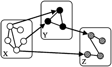
Figure 2: Block Directed MRFs: The joint distribution of $(X,Y,Z)$ can be written as $\mathbb{P}_{\exp}[X]\mathbb{P}_{\exp}[Y|X]\mathbb{P}_{\exp}[Z|X,Y]$

Then, one possible way of specifying a joint distribution, $\mathbb{P}(X,Y,Z)$ over these variables is given by the following BDMRF: $\mathbb{P}_{\exp}[X,Y,Z]=\mathbb{P}_{\exp}[X]\allowbreak\mathbb{P}_{\exp}[Y|X]\,\mathbb{P}_{\exp}[Z|X,Y]$. For pairwise graphical models, this distribution is denoted by directed edges extending from nodes in $X$ to nodes in $Z$ and $Y$ and from nodes in $Y$ to nodes in $Z$ as illustrated in Figure 2. We can write the form of this joint BDMRF distribution as follows:

$$\log\mathbb{P}[X,Y,Z]=\log\mathbb{P}_{\exp}[X]+\log\mathbb{P}_{\exp}[Y|X]+\log\mathbb{P}_{\exp}[Z|X,Y]$$

where $\mathbb{P}_{\exp}[X]$ is an Ising MRF, $\mathbb{P}_{\exp}[Y|X]$ is a Gaussian CRF as described earlier, and $\mathbb{P}_{\exp}[Z|X,Y]$ follows a Poisson CRF. When we specify linear covariate functions as in (14), these take the following forms:

$$\log\mathbb{P}_{\exp}[X]=\sum_{t\in V_{X}}\theta_{t}\,X_{t}+\sum_{(t,t^{\prime})\in E_{X}}\theta_{tt^{\prime}}\,X_{t}\,X_{t^{\prime}}-A_{X}(\theta)\,,$$

$$\log\mathbb{P}_{\exp}[Y|X]=\sum_{s\in V_{Y}}\Big{(}\theta_{s}+\sum_{t\text{ s.t }(s,t)\in E_{XY}}\theta_{st}\,X_{t}\Big{)}\frac{Y_{s}}{\sigma_{s}}+\sum_{(s,s^{\prime})\in E_{Y}}\frac{\theta_{ss^{\prime}}}{\sigma_{s}\sigma_{s^{\prime}}}\,Y_{s}\,Y_{s^{\prime}}$$

$$\hskip 56.9055pt-\sum_{s\in V_{Y}}\frac{Y_{s}^{2}}{2\sigma^{2}_{s}}-A_{Y|X}\big{(}\theta(X)\big{)}\,,$$

$$\log\mathbb{P}_{\exp}[Z|X,Y]=\sum_{u\in V_{Z}}\Big{(}\theta_{u}+\sum_{t\text{ s.t }(t,u)\in E_{XZ}}\theta_{tu}\,X_{t}+\sum_{s\text{ s.t }(s,u)\in E_{YZ}}\theta_{su}\,\frac{Y_{s}}{\sigma_{s}}\Big{)}Z_{u}$$

$$\hskip 56.9055pt+\sum_{(u,u^{\prime})\in E_{Z}}\theta_{uu^{\prime}}\,Z_{u}\,Z_{u^{\prime}}-\sum_{u\in V_{Z}}\log(Z_{u}!)-A_{Z|X,Y}\big{(}\theta(X,Y)\big{)}\,.$$

Notice that our BDMRF model is normalizable if each of the Ising MRF, Gaussian CRF and Poisson CRFs are normalizable. We discussed these conditions in Section 2.6; namely, $\Theta\prec 0$ for the Gaussian CRF as defined previously and $\theta_{uu^{\prime}}\leq 0$ for all $u,u^{\prime}\in V_{Z}$ for the Poisson CRF. This particular BDMRF formulation then exists and permits non-trivial dependencies between count-valued, continuous and binary-valued random vectors.

Even in this simple case of three homogeneous blocks of variables, we have given just one possible formulation of a BDMRF model and there exists a combinatorial number of ways to specify a valid BDMRF model in this case as the Ising CRF, Gaussian CRF, and Poisson CRF distributions exist under fairly mild conditions. Thus, even for fixed variable types, our BDMRFs allow for a most flexibly and rich class of dependence structures between data of mixed types. Furthermore, the recursive conditioning via our mixed CRFs substantially weakens the normalizability conditions so that non-trivial dependencies are permitted in many more cases such as our above example where the mixed MRF distribution does not permit dependencies between variables of different types.

Applicability of BDMRFs

To specify our BDMRF model, one must know both the block partitions of variables as well as the ordering of these blocks which determine the directionality of edges between nodes in different blocks. While these assumptions may seem restrictive, they naturally arise in many settings. For example, sets of variables measured over time naturally form blocks corresponding to each time point and the blocks can clearly be ordered according to a chain graph. Analogously, this natural ordering arises with applications to sequential treatments and natural language processing among many others.

While it may be less obvious, natural directionality between blocks of variables can also arise in settings that are not associated with time or sequences. Consider the example of different types of high-throughput genomics data measured on the same set of samples as previously discussed in Section 1. Here, we have mutations and aberrations (via SNPs and copy number aberrations) which are binary, gene expression (via RNA-sequencing) which are counts, and epigenetic markers (via methylation arrays) which are continuous. Thus, each set of genetic variables forms a natural block of binary sequence genetic markers, $X$, count-valued functional genetic markers, $Y$, and continuous epigenetic markers, $Z$. Biologically, however, scientists have established how these genomic variables interact with each other. For example, mutations and aberrations are fixed alterations in the DNA sequence that influence gene expression. An epigenetic marker or methylated region determines whether a sequence of DNA is ready for transcription, and thus also influences gene expression. Then based on scientific knowledge, we expect both mutation and methylation markers to point to gene expression markers, thus determining the directionality between these blocks of variables. Within these types of genomic biomarkers, however, we expect Markov conditional dependencies corresponding to undirected edges, which precisely correspond to the mixed graph construction underlying our BDMRFs.

4 Learning BDMRFs

Algorithm 1 Graph Selection Algorithm for BDMRFs

  Input: $n$ i.i.d. samples $\big{\{}X^{(j)}\big{\}}_{j=1}^{n}$ and the set of partial DAG orderings $\{V_{1},V_{2},\ldots,V_{m}\}$.

  for $i=1$ to $m$ do

     Learn conditional mixed CRF $\mathbb{P}_{\exp}[X_{V_{i}}|X_{\textnormal{PA}(i)}]$ via neighborhood selection.

  end for

  Output: $\mathbb{P}[X]=\prod_{i=1}^{m}\mathbb{P}_{\exp}[X_{V_{i}}|X_{\textnormal{PA}(i)}]$.

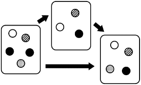
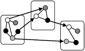
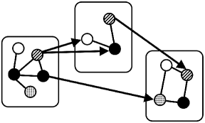
Figure 3: Graphical model structural learning. Given $n$ i.i.d. samples and the partial DAG orderings as in fgure (a), our goal is to recover the graphical model structure of underlying distribution such as in figure (b) or figure (c).

In this section, we investigate fitting our class of BDMRF models in (25) to data, under high-dimensional settings where the number of variables or nodes in the graph may potentially be larger than the number of samples. Specifically, suppose we observe $n$ i.i.d. samples $\big{\{}X^{(j)}\big{\}}_{j=1}^{n}$ from an underlying BDMRF distribution with unknown parameters $\theta^{*}$:

$$\log\mathbb{P}[X]=\sum_{i=1}^{m}\bigg{\{}\sum_{C\in\mathcal{C}_{V_{i}}}\theta^{*}_{C}(X_{\textnormal{PA}(i)})\prod_{s\in C}B_{s}(X_{s})+\sum_{s\in V_{i}}M_{s}(X_{s})-A_{i}\big{(}\theta^{*}(X_{\textnormal{PA}(i)})\big{)}\bigg{\}}.$$ (26)

Then, our objective is two-fold: (a) parameter learning, or to estimate the unknown parameters $\theta^{*}$, and (ii) structure learning, or to estimate the unknown edge-set $E$ of the underlying mixed graph. These tasks are frequently also referred to as graphical model estimation and selection respectively.

These two problems are especially challenging for our class of BDMRF models. As with classical MRFs, the normalization constant for BDMRF distributions is not available in closed form. Further, our class of distributions need not even belong to an exponential family as noted in earlier sections. Thus, estimating our class of models by directly maximizing the full likelihood is typically intractable. Secondly, the set of variables in our class of models is not only high-dimensional, but also heterogeneous, belonging to varied data-types. Lastly, the edge structure of the mixed graph underlying our class of BDMRF distributions have both directed and undirected edges - directed edges between variables from a parent block to variables in a child block, and undirected edges connecting variables within each block. Learning the structure of even solely directed edges of directed graphical models is known to be an NP-hard problem [25], unless a partial ordering of the variables is known [39]. Accordingly, in this paper, we assume that the partial ordering of the blocked DAG is known a-priori, based on domain knowledge. This assumption is especially relevant in areas such as high-throughput genomics, as we discussed in Section 3.3. Assuming these partial orderings over the DAG blocks, our learning task is reduced to recovering the undirected skeleton of the mixed graph in Figure 3.

By construction, our class of BDMRF distributions in (25) is completely specified by mixed CRF distributions (24) over the DAG blocks. Accordingly, we can reduce the problem of estimating the overall BDMRF distribution to that of estimating the corresponding mixed CRFs, as outlined in Algorithm 1. In order to learn any of the mixed CRFs $\mathbb{P}_{\exp}[X_{V_{i}}|X_{\textnormal{PA}(i)}]$, only the sample sub-vectors restricted to $X_{V_{i}}$ and $X_{\textnormal{PA}(i)}$ are required. Therefore, the overall BDMRF estimation problem can be reduced to the set of sub-problems of estimating the mixed CRFs comprising the BDMRF:

$$\log\mathbb{P}_{\exp}[X_{V_{i}}|X_{\textnormal{PA}(i)}]\propto\sum_{C\in\mathcal{C}_{V_{i}}}\theta^{*}_{C}(X_{\text{PA}(C)})\prod_{s\in C}B_{s}(X_{s})+\sum_{s\in V_{i}}M_{s}(X_{s}).$$ (27)

In the following, we focus on pairwise graphical models with linear covariate functions meaning that the parameter functions corresponding to node-wise cliques $C:=\{s\}$, have the following form:

$$\theta^{*}_{C}(X_{\textnormal{PA}(i)}):=\theta^{*}_{s}+\sum_{t\in\textnormal{PA}(s)}\theta^{*}_{st}\,B_{t}(X_{t}),$$ (28)

while the parameter functions corresponding to pair-wise cliques $C:=\{s,s^{\prime}\}$, will be simply a constant parameterized by $\theta^{*}_{ss^{\prime}}$:

$$\theta^{*}_{C}(X_{\textnormal{PA}(i)}):=\theta^{*}_{ss^{\prime}}.$$ (29)

Thus, overall the mixed CRF distribution in (27), when restricted to be pairwise, takes the form:

$$\log\mathbb{P}_{\exp}[X_{V_{i}}|X_{\textnormal{PA}(i)}]\propto \sum_{s\in V_{i}}\bigg{\{}\theta^{*}_{s}+\sum_{t\in\textnormal{PA}(s)}\theta^{*}_{st}\,B_{t}(X_{t})\bigg{\}}B_{s}(X_{s})$$

$$+\sum_{s^{\prime}\in V_{i}\text{ s.t. }(s,s^{\prime})\in E}\theta^{*}_{ss^{\prime}}\,B_{s}(X_{s})\,B_{s^{\prime}}(X_{s^{\prime}})+\sum_{s\in V_{i}}M_{s}(X_{s}).$$ (30)

As noted above, the task of estimating a BDMRF distribution from data reduces to the task of estimating these mixed CRFs (4); since the graph factors according to these mixed CRFs, we can estimate each one independently. We propose to do so following the node-wise neighborhood estimation approach of [34, 35, 47, 48], which allows us to side-step the task of computing the log-partition function of the mixed CRFs. These neighborhood selection approaches seek to learn the network structure through an $\ell_{1}$-norm penalty that sparsely estimates the set of edge parameters, the non-zeros of which correspond to the selected node-neighbors. Estimating the block mixed CRF (4) in turn reduces to estimating the univariate node-conditional distributions of variables $X_{s}$ for $s\in V_{i}$ given all other nodes in $V_{i}$ and $\textnormal{PA}(i)$: have the form:

$$\log\mathbb{P}_{\exp}[X_{s}|X_{V_{i}\setminus s}, X_{\textnormal{PA}(i)}]\propto\bigg{\{}\theta^{*}_{s}+\sum_{t\in\textnormal{PA}(s)}\theta^{*}_{st}\,B_{t}(X_{t})$$

$$+\sum_{s^{\prime}\in V_{i}\text{ s.t. }(s,s^{\prime})\in E}\theta^{*}_{ss^{\prime}}\,B_{s^{\prime}}(X_{s^{\prime}})\bigg{\}}B_{s}(X_{s})+M_{s}(X_{s}).$$ (31)

Therefore, for each node $X_{s}$ in $V_{i}$, the node-conditional distribution is specified by a parameter vector $\boldsymbol{\theta^{*}}(s)$ with three components $\boldsymbol{\theta^{*}}(s):=(\theta^{*}_{s},\boldsymbol{\theta^{*}}_{V_{i}},\boldsymbol{\theta^{*}}_{\textnormal{PA}(i)})$. Here, $\theta^{*}_{s}\in\mathbb{R}$ is the nodewise weight in the nodewise parameter function in (28). $\boldsymbol{\theta^{*}}_{V_{i}}:=\{\theta^{*}_{ss^{\prime}}\}_{s^{\prime}\in{V_{i}\backslash s}}\in\mathbb{R}^{p_{i}-1}$, where $p_{i}=|V_{i}|$, is the vector of intra-block edge-weights in the nodewise parameter function in (28). And finally, $\boldsymbol{\theta^{*}}_{\textnormal{PA}(i)}:=\{\theta^{*}_{st}\}_{t\in\textnormal{PA}(i)}\in\mathbb{R}^{q_{i}-1}$, where $q_{i}:=|\textnormal{PA}(i)|$, is the vector of inter-block edge weights in the pairwise parameter function in (29).

Let $\mathcal{N}^{*}_{V_{i}}(s)=\{s^{\prime}\in{V_{i}\backslash s}:\theta^{*}_{ss^{\prime}}\neq 0\}$ denote the set of true intra-block neighbors of $s\in V_{i}$. Let $d_{V_{i}}=\max_{s\in V_{i}}|\mathcal{N}^{*}_{V_{i}}(s)|$ denote the number of these intra-block neighbors. Similarly, let $\mathcal{N}^{*}_{\textnormal{PA}(i)}(s)=\{t\in\textnormal{PA}(i):\theta^{*}_{st}\neq 0\}$ denote the set of true inter-block neighbors of $s\in V_{i}$. Let $d_{\textnormal{PA}(i)}=\max_{s\in V_{i}}|\mathcal{N}^{*}_{\textnormal{PA}(i)}(s)|$ denote the number of these inter-block neighbors.

Then, given $n$ i.i.d. samples from our pairwise BDMRF of the form in (4) with unknown parameters, we estimate the node-conditional distributions in (4) by solving for the $\ell_{1}$-regularized conditional MLEs:

$$\min_{\boldsymbol{\theta}(s)\in\mathbb{R}^{1+p_{i}+q_{i}}}-\frac{1}{n}\sum_{j=1}^{n} \log\mathbb{P}\Big{(}X_{s}^{(j)}|X_{V_{i}\setminus s}^{(j)},X_{\textnormal{PA}(i)}^{(j)};\theta\Big{)}+\lambda\|\boldsymbol{\theta}_{V_{i}}\|_{1}+\mu\|\boldsymbol{\theta}_{\textnormal{PA}(i)}\|_{1}\,,$$ (32)

where $\lambda$, $\mu$ are regularization constants, with $\lambda$ determining the degree of sparsity in the connections between $X_{s}$ and $X_{V_{i}\setminus s}$, and $\mu$ determining the degree of sparsity in the connections between $X_{s}$ and the nodes in $\textnormal{PA}(i)$. Note that if the sufficient statistics are linear, $B_{s}(X_{s})=X_{s}$, then (32) can in turn be written in via exponential family natural parameters, $\boldsymbol{\beta}$, in the form of an $\ell_{1}$ regularized Generalized Linear Model as first presented in Yang et al. [46, 48]:

$$\min_{\boldsymbol{\beta}(s)\in\mathbb{R}^{1+p_{i}+q_{i}}} -\frac{1}{n}\sum_{j=1}^{n}\ell\left(X_{s}^{(j)};\beta_{s}+\sum_{t\in\textnormal{PA}(i)}\beta_{st}\,B_{t}\big{(}X_{t}^{(j)}\big{)}+\sum_{s^{\prime}\in V_{i}}\beta_{ss^{\prime}}\,B_{s^{\prime}}\big{(}X_{s^{\prime}}^{(j)}\big{)}\right)$$

$$+\lambda\|\boldsymbol{\beta}_{V_{i}}\|_{1}+\mu\|\boldsymbol{\beta}_{\textnormal{PA}(i)}\|_{1}\,.$$

Given the solution $\widehat{\boldsymbol{\theta}}(s)$ of the $M$-estimation problem (32) above, we can obtain an estimate of the true intra-block neighbors $\mathcal{N}^{*}_{V_{i}}(s)$ of a node $s\in V_{i}$ by:

$$\widehat{\mathcal{N}}_{V_{i}}(s)=\{s^{\prime}\in{V_{i}\backslash s}:\widehat{\boldsymbol{\theta}}_{ss^{\prime}}\neq 0\},$$

and obtain an estimate of the true inter-block neighbors $\mathcal{N}^{*}_{PA(i)}(s)$ of $s\in V_{i}$ by:

$$\widehat{\mathcal{N}}_{PA(i)}(s)=\{t\in\textnormal{PA}(i):\widehat{\boldsymbol{\theta}}_{st}\neq 0\}.$$

As we show below, these graph-structure estimates $\{\widehat{\mathcal{N}}_{V_{i}}(s),\widehat{\mathcal{N}}_{PA(i)}(s)\}$ from our $M$-estimator come with strong statistical guarantees.

Theorem 8.

Consider a pairwise mixed CRF distribution as specified in (4). Suppose we solve the $M$-estimation problem in (32) with the regularization parameters set as

$$\lambda\geq M_{1}\sqrt{\frac{\log p_{i}}{n}}\quad\mu\geq M_{1}\sqrt{\frac{\log q_{i}}{n}},\quad\textrm{and}\quad\max\{\lambda,\mu\}\leq M_{2},$$

where $M_{1}$ and $M_{2}$ are some constants that depend on the types of exponential family in (4). Further suppose that the minimum intra-block and inter-block edge-weights satisfy:

$$\min_{t\in V_{i}\setminus s\cup\textnormal{PA}(i)}|\theta_{st}^{*}|\geq\frac{10}{\rho_{\min}}\max\Big{\{}\lambda\sqrt{d_{V_{i}}}\,,\,\mu\sqrt{d_{\textnormal{PA}(i)}}\Big{\}},$$

where $\rho_{\min}$ is the minimum eigenvalue of the Hessian of the loss function at $\boldsymbol{\theta}^{*}(s)$, where we recall the notation that $p_{i}$ and $q_{i}$ are the number of intra-block and inter-block neighbors respectively of node $s\in V_{i}$. Then, for some universal positive constants $L$, $c_{1}$, $c_{2}$, and $c_{3}$, if

$$n\geq L\big{(}d_{V_{i}}+d_{\textnormal{PA}(i)}\big{)}^{2}\big{(}\log p_{i}+\log q_{i}\big{)}\Big{(}\max\big{\{}\log n,\log(p_{i}+q_{i})\big{\}}\Big{)}^{2},$$

then with probability at least $1-c_{1}\max\{n,p_{i}+q_{i}\}^{-2}-\exp(-c_{2}n)-\exp(-c_{3}n)$, the solution $\widehat{\boldsymbol{\theta}}$ of the M-estimation problem in (32) satisfies the following:

(a)

(Parameter Error) For each node $s\in V$, the solution $\widehat{\boldsymbol{\theta}}$ is unique with error bound:

$$\|\widehat{\boldsymbol{\theta}}_{\textnormal{PA}}-\boldsymbol{\theta}^{*}_{\textnormal{PA}}\|_{2}+\|\widehat{\boldsymbol{\theta}}_{V_{i}}-\boldsymbol{\theta}^{*}_{V_{i}}\|_{2}\leq\,\frac{5}{\rho_{\min}}\max\Big{\{}\lambda\sqrt{d_{V_{i}}}\,,\,\mu\sqrt{d_{\textnormal{PA}(i)}}\Big{\}}$$

(b)

(Structure Recovery in $V_{i}$) The solution recovers the true intra-block neighborhoods exactly, so that $\widehat{\mathcal{N}}_{V_{i}}(s)=\mathcal{N}^{*}_{V_{i}}(s)$, for all $s\in V_{i}$.

(c)

(Structure Recovery between $V_{i}$ and $\textnormal{PA}(i)$) The solution recovers the true inter-block neighborhoods exactly, so that $\widehat{\mathcal{N}}_{\textnormal{PA}(i)}(s)=\mathcal{N}^{*}_{\textnormal{PA}(i)}(s)$, for all $s\in V_{i}$.

Note that since the neighborhood of each node is recovered with high-probability, the entire graph structure estimate in turn is recovered exactly with high-probability, by a simple application of a union bound. These statistical guarantees extend the graph estimation and selection results from Yang et al. [46, 48] to our BDMRF setting.

5 Numerical Examples

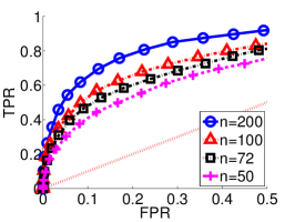
(a) Gau-Ising Mixed MRF

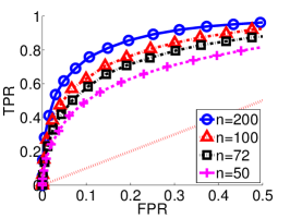
(b) Gau MRF-Ising CRF

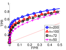
(c) Gau CRF-Ising MRF

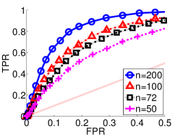
(d) Poi-Ising Mixed MRF

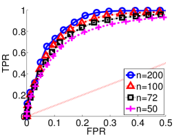
(e) Poi MRF-Ising CRF

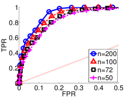
(f) Poi CRF-Ising MRF

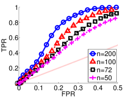
(g) Gau-TPGM Mixed MRF

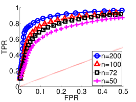
(h) Gau MRF-Poi CRF

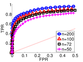
(i) Gau CRF-Poi MRF

Figure 4: Receiver Operator Characteristic (ROC) curves for graph selection of various examples of homogeneous mixed MRFs and our EBDMRFs whose form is specified by the MRF and CRF component as labeled(Gau indicates Guassian and Poi does Poisson). Data was generated from our models via Gibbs samplers with $p=72$ nodes on a lattice structure; curves are generated by varying the regularization parameter and shown for several samples sizes, $n$.

We first evaluate the performance of our $M$-estimator in the previous section for estimating our class of BDMRF models from data through a series of simulated numerical examples. All simulated examples used a two-dimensional lattice graph structure. Care was taken to ensure that all parameters meet normalizability conditions discussed in Section 2.5; specific parameter values for all our simulated examples are given in Appendix 8.6. We generated samples from the models via a Gibbs sampler based on the node conditional distributions specified in (4). Our $M$-estimator, based on $\ell_{1}$-penalized node-conditional maximum likelihood as described in Section 4, was implemented via projected gradient descent [4].

5.1 EBDMRFs

Our first set of simulations are for our class of Elementary Block Directed Markov Random Fields (EBDMRFs), with two blocks of variables, as described in Section 2. We constructed models with $p=72$ variables, with two blocks of $p_{x}=36$ and $p_{y}=36$ variables each. For various instances of our model, we generated datasets of four different sample sizes, $n=50,72,100,200$. We computed Receiver operator characteristic (ROC) curves for graph structure recovery averaged over 10 replicates by varying the regularization parameter as shown in Figure 4. The top two panels display graph structure recovery for three instances of our EBDMRF class of distributions $\mathbb{P}[X,Y]$ over the two blocks of variables $(X,Y)$, by varying the block-DAG over the two blocks. The left panels use a mixed MRF [50], where all the variables are in a single block, the middle panels use the decomposition $\mathbb{P}_{\exp}[Y|X]\,\mathbb{P}_{\exp}[X]$, while the right panels use the decomposition $\mathbb{P}[X,Y]=\mathbb{P}_{\exp}[X|Y]\,\mathbb{P}_{\exp}[Y]$, employing products of mixed CRFs and mixed MRFs. As the figure shows, our $M$-estimators (specified by the corresponding model) are able to recover the underlying network structure, even in high-dimensional sampling regimes.

The bottom panel in particular highlights the modeling advantages of our class of models when compared with the mixed MRFs [50]. As we have noted earlier in Section 2.6, the mixed MRF framework does not permit dependencies between Gaussian and Poisson type variables for reasons of normalizability. Our class of EBDMRF distributions, on the other hand, allow for such dependencies. Figure 4(h) and Figure 4(i) show graph structure recovery for EBDMRFs through Gaussian MRF-Poisson CRF, and Gaussian CRF-Poisson MRF, respectively; these represent instances where the corresponding mixed MRF does not permit inter-data-type dependencies. Figure 4(g) provides an additional way to model inter-data-type dependencies using the class of mixed MRFs, by using a truncated variant of the Poisson MRF instead as introduced in  [49]. Overall, as these simulations suggest, our class of EBDMRFs permit a wide class of normalizable distributions.

5.2 BDMRFs

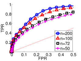
(a) $\mathbb{P}[X|Y,Z]\,\mathbb{P}[Y|Z]\,\mathbb{P}[Z]$

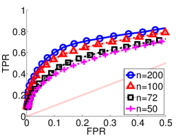
(b) $\mathbb{P}[Y|X,Z]\,\mathbb{P}[X|Z]\,\mathbb{P}[Z]$

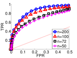
(c) $\mathbb{P}[Y|X]\,\mathbb{P}[X|Z]\,\mathbb{P}[Z]$

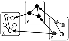
(d) DAG structure of (a)

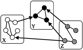
(e) DAG structure of (b)

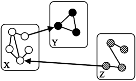
(f) DAG structure of (c)

Figure 5: Receiver Operator Characteristic (ROC) curves (top) for graphical structural learning for various configurations of our BDMRFs for three homogeneous blocks of variables: binary (Ising, $X$), continuous (Gaussian, $Y$) and counts (Poisson, $Z$). Model formulations with an illustrative picture are given in the bottom panel.

Our next set of simulations study graph selection recovery for our general class of BDMRF distributions with three homogeneous blocks of variables where we know the partial ordering over the variable blocks. Data was again generated via Gibbs sampler with a lattice graph structure connecting nearest neighbors on a two dimensional grid and with $p=75$ variables split into three blocks of $p_{X}=25$, $p_{Y}=25$, and $p_{Z}=25$ variables. In Figure 5, we plot ROC curves for graph structure recovery of three instances of our model with three blocks of variables: binary (for which we use Ising CRFs and MRFs), counts (for which we use Poisson CRFs and MRFs) and continuous (for which we use Gaussian CRFs and MRFs). The specific models with illustrated directionality are given in the bottom panel. These results show that our class of $M$-estimators are able to reasonably recover the underlying network even under extremely sample-limited settings. We note that as before, we cannot model dependencies between these three sets of variables in the classical mixed MRF framework for reasons of normalizability. Thus again, these illustrate the breadth and flexibility of our class of models.

5.3 BDMRFs: When the DAG Partial Ordering is Unknown

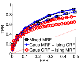
(a) Mixed MRF

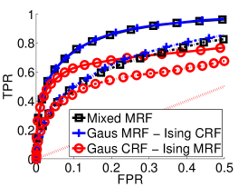
(b) Gaussian MRF-Ising CRF

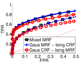
(c) Gaussian CRF-Ising MRF

Figure 6: Receiver Operator Characteristic (ROC) curves for graphical structural learning with two sets of homogeneous variables, binary (Ising) and continuous (Gaussian) when the true model (a) mixed MRF (b) Gaussian MRF-Ising CRF or (c) Gaussian CRF-Ising MRF, is unknown. Solid lines show the results for $n=200$ and dotted lines do for $n=50$.

In the previous simulations, and in the main section of the paper, we studied graph structure recovery assuming the partial ordering between the variable blocks of our BDMRF is known. Graph structure recovery when this partial ordering of the blocked DAG is unknown is a much more challenging problem. While a complete theoretical and empirical treatment of this question is beyond the scope of this paper, in this section, we provide brief numerical results demonstrating that even under this setting, recovering some dependencies is achievable via node-neighborhood estimation. In Figure 6, we plot ROC curves for graph structure recovery for BDMRFs with two blocks of variables, binary (corresponding to Ising CRF and MRF components), and continuous (corresponding Gaussian CRF and MRF components), for the same three BDMRF instances and simulations settings as in the top panel of Figure 4. Here however, for each of the model instances, we do not just present results for the $M$-estimator corresponding to the specific model instance, but for three different $M$-estimators corresponding to the three different model instances. As seen in the figure, the $M$-estimator corresponding to the true model is not always the best estimator under extremely sample-limited-settings (though we might expect it to be so as $n$ increases). As the plots in this brief investigation show, the $M$-estimator corresponding to the mixed MRF model may be the most robust to model misspecification, which in turn indicates that we could use this estimator to learn dependencies even when the true partial ordering between the variable blocks may be unknown or misspecified. A full study extending these preliminary results is left as a promising area of future work.

6 Case Study: High-Throughput Genomics

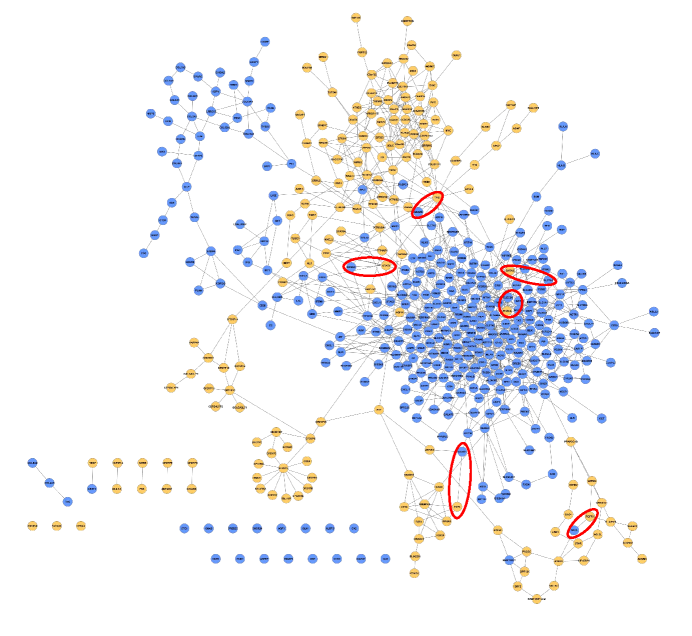
Figure 7: Invasive breast carcinoma network of gene expression (blue; counts via RNA-sequencing; $Y$) and genomic aberrations (yellow; binary via mutations and copy number aberrations; $X$) estimated via our BDMRF distribution. We learn the graph structure assuming the components $\mathbb{P}_{\exp}[Y|X]$ and $\mathbb{P}_{\exp}[X]$ are specified by a sub-linear Poisson CRF and an Ising MRF respectively. Our method discovered several biologically important connections between different types of biomarkers (circled in red).

We apply our class of BDMRF models to high-throughput cancer genomics data to find connections both within and between different types of biomarkers. Specifically, we study how genomic aberrations, which include both SNPs and copy number variations, affect gene expression levels. Note that the standard method for finding connections between mutations and expression levels, commonly called expression Quantitative Trait Loci (eQTL) analysis [29], uses regression models to find connections between the two different types of biomarkers but cannot model the connections within the set of mutations and gene expression levels.

For our analysis, we use publicly available data on invasive breast carcinoma available from the Cancer Genome Atlas (TCGA) [6]. Level III RNA-sequencing data for 806 patients was downloaded and pre-processed using techniques described in Allen and Liu [1], so that the expression levels can be well-modeled with the Poisson distribution. For the aberration data, we used Level II non-silent somatic mutations and Level III copy number variation data for 951 patients. The later was segmented using standard techniques [52] and merged with the mutation data at the gene level to form a binary matrix, indicating whether a mutation or copy number aberration is present or absent in the coding region of the gene. This leaves us with $n=697$ patients that are common to both the gene expression, $Y$, and aberration, $X$, data sets. We filtered the biomarkers further to consider the top 2% of genes whose expression levels had the highest variance across patients, $p_{X}=329$, and only the aberrations present in at least 10% of patients, $p_{Y}=169$, yielding $p=498$ total biomarkers.

We fit our BDMRF model to this data to learn the structure of the breast cancer genomic network. As we know that aberrations affect expression levels but not the converse, we set the partial ordering of the mixed graph underlying our BDMRF to have the aberration variable block ordered before the expression level variable block. Specifically, we used the factorization $\mathbb{P}[X,Y]=\mathbb{P}_{\exp}[Y|X]\mathbb{P}_{\exp}[X]$, where $\mathbb{P}_{\exp}[Y|X]$ is a pairwise Poisson conditional random field as RNA-sequencing data is count-valued and $\mathbb{P}_{\exp}[X]$ is a pair-wise Ising model as aberration data is binary. Recall that for the Poisson MRF or CRF, only negative conditional dependencies are permitted, which is unrealistic for genomics data. Thus, instead of the usual Poisson CRF, we fit a Sub-Linear Poisson CRF, an extension of the Sub-Linear Poisson MRF model described in Yang et al. [49], which uses a sub-linear function as the exponential family sufficient statistic to relax the resulting normalizability conditions, permitting both positive and negative conditional dependencies; see Yang et al. [49] for further details. Node-wise neighborhood selection as described in Section 4 was employed to learn the edge structure of the network. Stability selection, as described in Liu et al. [32], was used with parameter level $\beta=0.01$ to determine the optimal level of regularization.

Our estimated network is presented in Figure 7 where blue nodes denote gene expression biomarkers and yellow nodes denote aberration biomarkers. Our network identified several key connections between biomarkers of different types; these are denoted via red circles in Figure 7. These include both links that have been previously indicated in the literature, as well as some novel discoveries. First, several connections that we identify are well-known breast cancer biomarkers: the GATA3 mutation is linked to SLC39A6 expression; the ratio of these gene’s expressions levels are used to define breast cancer sub-types [21] and both of these biomarkers have been previously implicated in breast cancer [43]. The FGFR1 mutation is linked to PEG3 expression; the former regulates growth factors that are known to be amplified in breast cancer [19] while the latter modulates the related process of cancer progression [41]. The STAT3 mutation is linked to ERBB2 expression; these are known to be amplified in HERB2 sub-types [9].

Our estimated network also discovers several novel connections to be investigated and further validated in future work; these include: the TP53 mutation is linked to ADAM6 expression; TP53 is a well known tumor suppressor gene [30] and ADAM6 is a long non-coding RNA over-expressed in breast cancer [38]. The FGF3 mutation is linked to CCND1 expression; FGF3 regulates estrogen expanding breast cancer stem cells [15] and CDN1 leads to over-expression of hormone receptors in breast cancer [3]. The PIK3CA mutation is linked to CLEC3A expression and NAT1 expression; PIK3CA is a known oncogene [10], CLEC3A affects tumor metastasis [42], and NAT1 is a potential marker for the estrogen receptor positive sub-type [23].

Overall, this genomics example demonstrates the direct applicability of our class of BDMRF models for learning relevant connections both within and between cancer biomarkers of different types.

7 Discussion

In this paper, we have constructed a general class of mixed graphical models through block directed exponential family mixed conditional random fields. Our work generalizes much of the existing literature on parametric Markov Random Field (MRF) and Conditional Random Field (CRF) distributions, all of which are special cases of our framework. Our so-called class of Block Directed Markov Random Fields (BDMRFs) are an extremely flexible class of models, that are represented by mixed graphs, with both directed edges (through a DAG over blocks of variables) and undirected edges (within these blocks), between mixed types of variables. We have also shown that these are normalizable under fairly relaxed conditions.

To our knowledge, these models represent the first class of multivariate densities over mixed variables that directly permits and parameterizes such a rich set of dependencies. Our work thus has broad implications for multivariate analysis in general, especially that involving integrative analysis of mixed variables. At the very least, we have greatly expanded the class of off-the-shelf graphical models beyond canonical instances such as Ising and Gaussian graphical models, and have also provided estimators for our class of models that come with strong statistical guarantees even under high-dimensional settings.

While the main contributions of this paper are theoretical in nature, our novel class of BDMRF distributions has broad applicability in a variety of fields that yield mixed, big data. Beyond the high-throughput genomics example discussed in this paper, these include imaging genetics, national security, climate studies, spatial statistics, Internet data, marketing and advertising, and economics, among many others.

There are several avenues for further research building on the work in this paper. These include providing a goodness of fit test for understanding whether our models are applicable to any particular data set. Yang et al. [47] discuss a heuristic for this, but further work needs to be done to develop a proper post selection inferential procedure. While we have shown that our BDMRF distributions impose fairly relaxed conditions upon their parameters for normalizability, these conditions can still be limiting in practice, and more work is needed on general strategies for relaxing these normalizability conditions; for instance, this could be achieved by potentially extending the work in [49] on relaxing normalizability conditions for Poisson MRFs. Additionally, our work has concentrated on constructing models via single-parameter univariate exponential family distributions, which can be further extended to the case of multi-parameter exponential families. Finally, in this paper, we assumed that the partial ordering or DAG over the variable blocks is known a priori based on domain knowledge. For mixed genomics data, this assumption is realistic as we know how various biomarkers affect each other in the biological system. For other application areas, the directionality of links between blocks of variables may be unknown or the block designations of the variables may be unknown. In these situations, the question remains: can we still learn the dependence structure between mixed variables and/or estimate both the edges are their directionality? Our final set of simulations in Figure 5 suggests that we may be able to learn dependencies even if the true underlying BDMRF is unknown; further theoretical and empirical investigations that build on these are needed. Also, while there are several popular algorithms for learning DAGs [20], little is known about estimating MRFs with mixed directed and undirected edges, an open area of future research.

Overall, we have proposed a novel class of distributions for mixed variables, that has broad theoretical and practical implications across many statistical and scientific domains.

8 Appendix

8.1 Proof of Theorem 2

We follow the proof policy of [46, 48]: Define $Q({Y}|X)$ as

$$Q({Y}|X):=\log(\mathbb{P}[{Y}|X]/\mathbb{P}[{\bf 0}|X]),$$

for any ${Y}=(Y_{1},\ldots,Y_{p})\in\mathcal{Y}^{p}$ given $X$ where ${\bf 0}$ indicates a zero vector (The number of zeros vary appropriately in the context below). For any ${Y}$, also denote $\makebox[0.0pt][l]{\hskip 1.02495pt\rule[8.12498pt]{5.67886pt}{0.43057pt}}{Y}_{s}:=(Y_{1},\ldots,Y_{s-1},0,Y_{s+1},\ldots,Y_{p})$.

Now, consider the following general form for $Q({Y}|X)$:

$$Q({Y}|X)= \sum_{t_{1}\in V}Y_{t_{1}}G_{t_{1}}\big{(}Y_{t_{1}},X\big{)}+\ldots+$$ (33)

$$\sum_{t_{1},\ldots,t_{k}\in V}Y_{t_{1}}\ldots Y_{t_{k}}G_{t_{1},\ldots,t_{k}}\big{(}Y_{t_{1}},\ldots,Y_{t_{k}},X\big{)},$$

where $k$ is the maximum clique size of $G_{Y}$. It can then be seen that

$$\exp\Big{(}Q({Y}|X)-Q(\makebox[0.0pt][l]{\hskip 1.02495pt\rule[8.12498pt]{5.67886pt}{0.43057pt}}{Y}_{s}|X)\Big{)}=\mathbb{P}[{Y}|X]/\mathbb{P}[\makebox[0.0pt][l]{\hskip 1.02495pt\rule[8.12498pt]{5.67886pt}{0.43057pt}}{Y}_{s}|X]$$

$$=\ \frac{\mathbb{P}[Y_{s}|Y_{1},\ldots,Y_{s-1},Y_{s+1},\ldots,Y_{p},X]}{\mathbb{P}[0|Y_{1},\ldots,Y_{s-1},Y_{s+1},\ldots,Y_{p},X]},$$ (34)

where the first equality follows from the definition of $Q$, and the second equality follows from some algebra. Now, consider simplifications of both sides of (8.1). Given the form of $Q({Y}|X)$ in (33), we have

$$Q({Y}|X)-Q(\makebox[0.0pt][l]{\hskip 1.02495pt\rule[8.12498pt]{5.67886pt}{0.43057pt}}{Y}_{1}|X)=$$ (35)

$$Y_{1}\bigg{(}G_{1}\big{(}Y_{1},X\big{)}+\sum_{t=2}^{p}Y_{t}G_{1t}\big{(}Y_{1},Y_{t},X\big{)}+\ldots+$$

$$\sum_{t_{2},\ldots,t_{k}\in\{2,\ldots,p\}}Y_{t_{2}}\ldots Y_{t_{k}}G_{1,t_{2},\ldots,t_{k}}\big{(}Y_{1},\ldots,Y_{t_{k}},X\big{)}\bigg{)}.$$

Also, given the exponential family form of the node-conditional distribution specified in (9), we obtain

$$\log\frac{\mathbb{P}[Y_{s}|Y_{1},\ldots,Y_{s-1},Y_{s+1},\ldots,Y_{p},X]}{\mathbb{P}[0|Y_{1},\ldots,Y_{s-1},Y_{s+1},\ldots,Y_{p},X]}=$$ (36)

$$E_{s}(Y_{V\backslash s},X)(B_{s}(Y_{s})-B_{s}(0))+(C_{s}(Y_{s})-C_{s}(0)).$$

Setting $Y_{t}=0$ for all $t\neq s$ in (8.1), and using the expressions for the left and right hand sides in (35) and (36), we obtain,

$$Y_{s}G_{s}\big{(}Y_{s},X\big{)}$$

$$=\ E_{s}({\bf 0},X)(B_{s}(Y_{s})-B_{s}(0))+(C_{s}(Y_{s})-C_{s}(0)).$$

Setting $Y_{r}=0$ for all $r\not\in\{s,t\}$,

$$Y_{s}G_{s}\big{(}Y_{s},X\big{)}+Y_{s}Y_{t}G_{st}\big{(}Y_{s},Y_{t},X\big{)}$$

$$=\ E_{s}({\bf 0},Y_{t},{\bf 0},X)(B_{s}(Y_{s})-B_{s}(0))+(C_{s}(Y_{s})-C_{s}(0)).$$

Combining these two equations yields

$$Y_{s}Y_{t}G_{st}\big{(}Y_{s},Y_{t},X\big{)}$$

$$=\ \big{(}E_{s}({\bf 0},Y_{t},{\bf 0},X)-E_{s}({\bf 0},X)\big{)}(B_{s}(Y_{s})-B_{s}(0)).$$ (37)

Similarly, from the same reasoning for node $t$, we have

$$Y_{t}G_{t}\big{(}Y_{t},X\big{)}+Y_{s}Y_{t}G_{st}\big{(}Y_{s},Y_{t},X\big{)}$$

$$=\ E_{t}({\bf 0},Y_{s},{\bf 0},X)(B_{t}(Y_{t})-B_{t}(0))+(C_{t}(Y_{t})-C_{t}(0)),$$

and at the same time,

$$Y_{s}Y_{t}G_{st}\big{(}Y_{s},Y_{t},X\big{)}$$

$$=\ \big{(}E_{t}({\bf 0},Y_{s},{\bf 0},X)-E_{t}({\bf 0},X)\big{)}(B_{t}(Y_{t})-B_{t}(0)).$$ (38)

From the assumption of the statement of (8), $E_{s}(\cdot)$ depends $X$ only through $N_{YX}(s)$, and similarly $E_{t}(\cdot)$ does only through $N_{YX}(t)$. Furthermore, by the equality of (8.1) and (8.1), we obtain

$$E_{t}({\bf 0},Y_{s},{\bf 0},X)-E_{t}({\bf 0},X)=\frac{E_{s}({\bf 0},Y_{t},{\bf 0},X)-E_{s}({\bf 0},X)}{B_{t}(Y_{t})-B_{t}(0)}(B_{s}(Y_{s})-B_{s}(0)).$$ (39)

Since (39) should hold for all possible combinations of $Y_{s}$, $Y_{t}$ and $N_{YX}(s)\cap N_{YX}(t)$, for any fixed $Y_{t}\neq 0$,

$$E_{t}({\bf 0},Y_{s},{\bf 0},X)-E_{t}({\bf 0},X)=\theta_{st}\big{(}N_{YX}(s)\cap N_{YX}(t)\big{)}(B_{s}(Y_{s})-B_{s}(0))$$ (40)

where $\theta_{st}(\cdot)$ is a function on $N_{YX}(s)\cap N_{YX}(t)$. Plugging (40) back into (8.1),

$$Y_{s}Y_{t}G_{st}\big{(}Y_{s},Y_{t},X\big{)}$$

$$=\ \theta_{st}\big{(}N_{YX}(s)\cap N_{YX}(t)\big{)}(B_{s}(Y_{s})-B_{s}(0))(B_{t}(Y_{t})-B_{t}(0)).$$

More generally, by considering non-zero triplets, and setting $Y_{r}=0$ for all $r\not\in\{s,t,u\}$, we obtain,

$$Y_{s}G_{s}\big{(}Y_{s},X\big{)}+Y_{s}Y_{t}G_{st}\big{(}Y_{s},Y_{t},X\big{)}$$

$$+Y_{s}Y_{u}G_{su}\big{(}Y_{s},Y_{u},X)+Y_{s}Y_{t}Y_{u}G_{stu}\big{(}Y_{s},Y_{t},Y_{u},X\big{)}$$

$$=\, E_{s}({\bf 0},Y_{t},{\bf 0},Y_{u},{\bf 0},X)(B_{s}(Y_{s})-B_{s}(0))$$

$$+(C_{s}(Y_{s})-C_{s}(0)),$$

so that by a similar reasoning we can obtain

$$Y_{s}Y_{t}Y_{u}G_{stu}\big{(}Y_{s},Y_{t},Y_{u},X\big{)}=$$

$$\theta_{stu}\big{(}N_{YX}(s)\cap N_{YX}(t)\cap N_{YX}(u)\big{)}(B_{s}(Y_{s})-B_{s}(0))(B_{t}(Y_{t})-B_{t}(0))(B_{u}(Y_{u})-B_{u}(0)).$$

More generally, we can show that

$$Y_{t_{1}}\ldots Y_{t_{k}}G_{t_{1},\ldots,t_{k}}\big{(}Y_{t_{1}},\ldots,Y_{t_{k}},N_{Y}(X)\big{)}=$$

$$\theta_{t_{1},\ldots,t_{k}}\big{(}\cap_{t=t_{1},\ldots,t_{k}}N_{YX}(t)\big{)}(B_{t_{1}}(Y_{t_{1}})-B_{t_{1}}(0))\ldots(B_{t_{k}}(Y_{t_{k}})-B_{t_{k}}(0)).$$

Thus, the $k$-th order factors in the joint distribution as specified in (33) are tensor products of $(B_{s}(Y_{s})-B_{s}(0))$, thus proving the statement of the theorem.

8.2 Proof of Theorem 3 and 6

The joint distribution (11) factors according to $E_{X}$ and $E_{Y}$ by construction. Hence, (a) and (b) hold by Hammersley-Clifford theorem. Now, suppose that $\{d\}\cup C$ is not complete with respect to $G$. Then, since $C$ is complete and every node in $d$ is fully connected to $C$, we can conclude that again by Hammersley-Clifford theorem, $\theta_{C,d}(X)$ is decomposable $\sum_{j=1}^{i}\theta_{C,d_{j}}(X)$ where $d_{1},\ldots,d_{i}$ are the disjoint sets such that $\cup_{j=1,\ldots,i}{d_{j}}=d$ and $d_{j}\cup C$ is complete with respect to $G$ for all $j$, which means $\theta_{C,d}(X)=0$.

The proof of Theorem 6 can be trivially derived by extending this proof.

8.3 Proof of Theorem 4

We first introduce shorthand notations for unnormalized probabilities:

$$U_{X}=\exp\Big{(}\sum_{C\in\mathcal{C}_{X}}\theta_{C}\prod_{t\in C}B_{t}(X_{t})+\sum_{t\in V_{X}}M_{t}(X_{t})\Big{)}\,,$$

$$U_{XY}=\exp\Big{(}\sum_{C\in\mathcal{C}_{Y}}\theta_{C}\big{(}X_{N_{YX}(C)}\big{)}\prod_{s\in C}B_{s}(Y_{s})+\sum_{s\in V_{Y}}M_{s}(Y_{s})-A_{Y|X}\big{(}\theta\big{)}\Big{)}\,.$$

Suppose that $\mathbb{P}_{\exp}[X]$ and $\mathbb{P}_{\exp}[Y|X]$ are well-defined and normalizable, which means that $\sum_{X}U_{X}<\infty$, and $\sum_{Y}U_{XY}<\infty$ for any $X$. Note that $\sum$ operator can be substituted by integral for continuous case. Then, the log partition function of (11) can be shown to be finite as follows:

$$\sum_{X,Y}\Big{[}U_{X}U_{XY}\Big{]}=\sum_{X}\Big{[}U_{X}\big{(}\sum_{Y}U_{XY}\big{)}\Big{]}$$

$$\leq\, \sum_{X}\Big{[}U_{X}\max_{X}\big{(}\sum_{Y}U_{XY}\big{)}\Big{]}=\Big{[}\max_{X}\sum_{Y}U_{XY}\Big{]}\,\Big{[}\sum_{X}U_{X}\Big{]}<\infty.$$

8.4 Proof of Theorem 5

Since the unnormalized probability mass $\exp\{F(X;\theta)+F(X,Y;\theta)\}$ is strictly positive, $\exp\{F(X;\theta)\}>0$ and $\exp\{F(X,Y;\theta)\}>0$ for any $(X,Y)\in\mathcal{X}^{q}\times\mathcal{Y}^{p}$.

Suppose that $A(\theta)=\log\sum_{X}\Big{[}\exp\{F(X;\theta)\}\sum_{Y}\exp\{F(X,Y;\theta)\}\Big{]}<\infty$ as in the statement. Then, for any $X\in\mathcal{X}^{q}$, the partial summation of $A(\theta)$, $\exp\{F(X;\theta)\}\sum_{Y}\exp\{F(X,Y;\theta)\}$ is also summable;

$$\exp\{F(X;\theta)\}\sum_{Y}\exp\{F(X,Y;\theta)\}=c_{1},$$

which implies that $\sum_{Y}\exp\{F(X,Y;\theta)\}=c_{1}/\exp\{F(X;\theta)\}<\infty$, and $A_{Y|X}\big{(}\vartheta(X)\big{)}$ is summable.

Now, we consider the second term $A_{X}(\theta)$ in (2.4). Since $\exp\{F(X,Y;\theta)\}>0$ for any $X\in\mathcal{X}^{q}$, $\min_{X}\sum_{Y}\exp\{F(X,Y;\theta)\}$ is strictly positive; let us define $c_{\min}:=\min_{X}\sum_{Y}\exp\{F(X,Y;\theta)\}>0$. We then have:

$$c_{\min}\sum_{X}\exp\{F(X;\theta)\}=\sum_{X}\Big{[}c_{\min}\exp\{F(X;\theta)\}\Big{]}$$

$$\leq\, \sum_{X}\Big{[}\exp\{F(X;\theta)\}\sum_{Y}\exp\{F(X,Y;\theta)\}\Big{]}.$$

Therefore,

$$\sum_{X}\exp\{F(X;\theta)\}\leq\frac{1}{c_{\min}}\sum_{X}\Big{[}\exp\{F(X;\theta)\}\sum_{Y}\exp\{F(X,Y;\theta)\}\Big{]}.$$

Since $c_{\min}>0$ and $\Big{[}\exp\{F(X;\theta)\}\sum_{Y}\exp\{F(X,Y;\theta)\}\Big{]}<\infty$ by assumption, we can conclude $A_{X}(\theta)<\infty$, which completes the proof.

8.5 Normalizability of Mixed CRFs

The normalizability conditions for the mixed MRF $\mathbb{P}_{\exp}[X]$ is well developed in Yang et al. [50]. This can be seamlessly extended for the mixed CRF (10) case as well.

Proposition 1.

Suppose that some random variables in $Y$ are finite. Let $Z$ be a set of such random variables: $\mathcal{Z}_{s}$ is finite, with $\max\{z:z\in\mathcal{Z}_{s}\}<\infty$ and $\min\{z:z\in\mathcal{Z}_{s}\}>-\infty$. We also define $W$ to denote the remaining (infinite) random variables in $Y$ so that $Y=(Z,W)$. Suppose that the following conditional distribution given $Z$ is well-defined (i.e. normalizable) for all possible $Z\in\prod_{s\in V_{Z}}\mathcal{Z}_{r}$:

$$\log\mathbb{P}_{\exp}[W|Z,X]\propto\sum_{C\in\mathcal{C}_{W}}\theta_{C}(Z,X)\prod_{s\in C}B_{s}(W_{s})+\sum_{s\in V_{W}}M_{s}(W_{s}).$$

Then, $\mathbb{P}_{\exp}[W|Z,X]$ is normalizable if and only if mixed CRF $\mathbb{P}_{\exp}[Y|X]$ (10) is normalizable.

Proposition 2.

Suppose that all domains $\mathcal{Y}_{s}$ for $Y$ are infinite, and that the maximum size of cliques is limited to two with linear sufficient statistics $B_{s}(Y_{s})=Y_{s}$ for $\forall s\in V_{Y}$. Then the mixed CRF in (10) is normalizable only if at least one of the following conditions is satisfied for all $s,t\in V_{Y}$ with non-zero $\theta_{st}(X)$:

(a)

Both $\mathcal{Y}_{s}$ and $\mathcal{Y}_{t}$ are infinite only from one side, so that $\sup\{y:y\in\mathcal{Y}_{s}\}<\infty$ or $\inf\{y:y\in\mathcal{Y}_{s}\}>-\infty$, and similarly for $\mathcal{Y}_{t}$.

(b)

For all $\alpha,\beta>0$ such that $-M_{s}(Y_{s})=O(Y_{s}^{\alpha})$ and $-M_{t}(Y_{t})=O(Y_{t}^{\beta})$, it holds that $(\alpha-1)(\beta-1)\geq 1$.

Even though Proposition 1 and 2 are simply the generalization of analogous results on normalizability conditions of mixed MRF [50], they are useful to study to better understand why our BDMRF formulations are less restrictive than mixed MRFs. In Proposition 2, consider that conditions (a) and (b) only depend on the response variables $Y$ instead of both $X$ and $Y$. This can dramatically relax normalizability restrictions in many settings. For example, consider the Gaussian-Poisson EBDMRF studied in Section 2.6 for Poisson-associated variables $X$ and Gaussian-associated variables $Y$. For the mixed MRF, $\mathbb{P}_{\exp}[X,Y]$, we would consider both $X$ and $Y$ as response variables and neither (a) nor (b) in Proposition 2 hold. (For (a), $Y_{s}$ is not infinite only from one side, and for (b), $-M_{s}(Y_{s})=O(Y_{s}^{2})$ and $-M_{t}(X_{t})=O(X_{t}^{1.5})$, $(2-1)(1.5-1)$ is not larger than $1$). Hence, the Gaussian-Poisson mixed MRF is not normalizable.

On the other hand, both of our EBDMRF formulations are normalizable because of the relaxed restrictions with our mixed CRFs. Consider taking the variables $X$ and $Y$ to be two homogeneous blocks. Then the conditions in Proposition 2 need only to be satisfied for $X$ or $Y$. For the Gaussian-Poisson case, the statement in (a) holds for the Poisson CRF, $\mathbb{P}_{\exp}[X|Y]$ as all Poisson variables $X$ are unbounded in only one direction. Similarly, statement (b) holds for the Gaussian CRF, $\mathbb{P}_{\exp}[Y|X]$ since $-M_{s}(Y_{s})=O(Y_{s}^{2})$ for all Gaussian variable $Y_{s}$. (Further conditions on the normalizability of these Poisson and Gaussian CRFs are given in Section 2.6). Hence, both the Poisson and Gaussian CRFs are normalizable meaning that both of our EBDMRF formulations, $\mathbb{P}_{\exp}[X|Y]\mathbb{P}_{\exp}[Y]$ and $\mathbb{P}_{\exp}[Y|X]\mathbb{P}_{\exp}[X]$, are normalizable and permit dependencies in Gaussian-Poisson mixed graphical models.

8.6 Simulation Settings

Figure 8: Lattice Graph Structure

Table 1: Parameters used in data generation for various examples of homogeneous mixed MRFs and our EBDMRFs in Figure 4 whose form is specified by the MRF and CRF component as labeled.

Model	$\theta_{xx}$	$\theta_{yy}$	$\theta_{xy}$
Gaussian (X) - Ising (Y) Mixed MRF	0.2	0.3	0.1
Gaussian MRF - Ising CRF	0.5	0.3	0.1
Gaussian CRF - Ising MRF	0.5	0.3	0.1
Poisson (X) - Ising (Y) Mixed MRF	-0.8	0.4	0.6
Poisson MRF - Ising CRF	-0.8	0.4	0.6
Poisson CRF - Ising MRF	-0.8	0.4	0.6
Gaussian (X) CRF - TPGM (Y) MRF	0.1	0.1	0.2
Gaussian (X) MRF - Poisson (Y) CRF	0.6	-1	1
Gaussian (X) CRF - Poisson (Y) MRF	0.6	-1	1

Table 2: Parameters used in data generation for various configurations of our BDMRFs in Figure 5, for three homogeneous blocks of variables: binary (Ising, X), continuous (Gaussian, Y) and counts (Poisson, Z).

Model	$\theta_{xx}$	$\theta_{yy}$	$\theta_{zz}$	$\theta_{xy}$	$\theta_{xz}$	$\theta_{yz}$
$\mathbb{P}_{\exp}[X|Y,Z]\,\mathbb{P}_{\exp}[Y|Z]\,\mathbb{P}_{\exp}[Z]$	0.1	0.3	-0.8	0.1	0.1	0.1
$\mathbb{P}_{\exp}[Y|X,Z]\,\mathbb{P}_{\exp}[X|Z]\,\mathbb{P}_{\exp}[Z]$	0.1	0.3	-0.8	0.1	0.1	0.1
$\mathbb{P}_{\exp}[Y|X]\,\mathbb{P}_{\exp}[X|Z]\,\mathbb{P}_{\exp}[Z]$	0.1	0.3	-0.8	0.1	-	0.1

We generate samples from our BDMRF models using Gibbs sampling for the lattice network structure shown in Figure 8. Parameters for each model were specified as constant edge weights for each block corresponding to the values given in Table 1 and Table 2.

8.7 Genomics Case Study Comparisons

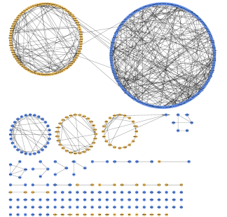
(a) EBDMRF

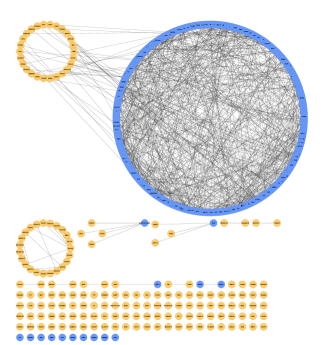
(b) Mixed MRF

Figure 9: Comparison of breast cancer genomics networks estimated via our EBDMRF vs. the mixed MRF.

In circle plots in Figure 9, we compare our EBDMRF network estimate to that of the mixed MRF network studied in [50] and reviewed in Section 1.2. We see that the mixed MRF finds many connections within gene expression biomarkers, but few within aberration biomarkers. In contrast, our BDMRF model finds both within connections as well as a few key between connections. Biologically, this result is not surprising as gene expression levels are known to be highly dependent, and thus when conditioning on all biomarkers as in the mixed MRF, connections within gene expressions dominate. With our network, conditioning based on the directions of known biological influence (i.e. aberrations influence gene expression), allows us to estimate a more biologically meaningful network.

References

- Allen and Liu [2013] G. I. Allen and Z. Liu. A local poisson graphical model for inferring networks from sequencing data. IEEE transactions on nanobioscience, 12(3):189, 2013.
- Argyriou et al. [2007] A. Argyriou, T. Evgeniou, and M. Pontil. Multi-task feature learning. Advances in neural information processing systems, 19:41, 2007.
- Arnold and Papanikolaou [2005] A. Arnold and A. Papanikolaou. Cyclin d1 in breast cancer pathogenesis. Journal of Clinical Oncology, 23(18):4215–4224, 2005.
- Beck and Teboulle [2009] A. Beck and M. Teboulle. A fast iterative shrinkage-thresholding algorithm for linear inverse problems. SIAM Journal on Imaging Sciences, 2(1):183–202, 2009.
- Besag [1974] J. Besag. Spatial interaction and the statistical analysis of lattice systems. Journal of the Royal Statistical Society. Series B (Methodological), pages 192–236, 1974.
- Cancer Genome Atlas Research Network [2012] Cancer Genome Atlas Research Network. Comprehensive molecular portraits of human breast tumours. Nature, 490(7418):61–70, 2012.
- Chen et al. [2014] S. Chen, D. Witten, and A. Shojaie. Selection and estimation for mixed graphical models. Arxiv preprint arXiv:1311.0085, 2014.
- Cheng et al. [2013] J. Cheng, E. Levina, and J. Zhu. High-dimensional mixed graphical models. arXiv preprint arXiv:1304.2810, 2013.
- Chung et al. [2014] S. S. Chung, N. Giehl, Y. Wu, and J. V. Vadgama. Stat3 activation in her2-overexpressing breast cancer promotes epithelial-mesenchymal transition and cancer stem cell traits. International journal of oncology, 44(2):403, 2014.
- Cizkova et al. [2012] M. Cizkova, A. Susini, S. Vacher, G. Cizeron-Clairac, C. Andrieu, K. Driouch, E. Fourme, R. Lidereau, and I. Bièche. Pik3ca mutation impact on survival in breast cancer patients and in era, pr and erbb2-based subgroups. Breast Cancer Res, 14:R28, 2012.
- Clifford [1990] P. Clifford. Markov random fields in statistics. In G. Grimmett and D. J. A. Welsh, editors, Disorder in physical systems. Oxford Science Publications, 1990.
- Cressie and Cassie [1993] N. A. Cressie and N. A. Cassie. Statistics for spatial data, volume 900. Wiley New York, 1993.
- Dobra and Lenkoski [2011] A. Dobra and A. Lenkoski. Copula gaussian graphical models and their application to modeling functional disability data. The Annals of Applied Statistics, 5(2A):969–993, 2011.
- Fellinghauer et al. [2013] B. Fellinghauer, P. Bühlmann, M. Ryffel, M. Von Rhein, and J. D. Reinhardt. Stable graphical model estimation with random forests for discrete, continuous, and mixed variables. Computational Statistics & Data Analysis, 64:132–152, 2013.
- Fillmore et al. [2010] C. M. Fillmore, P. B. Gupta, J. A. Rudnick, S. Caballero, P. J. Keller, E. S. Lander, and C. Kuperwasser. Estrogen expands breast cancer stem-like cells through paracrine fgf/tbx3 signaling. Proceedings of the National Academy of Sciences, 107(50):21737–21742, 2010.
- Frydenberg and Lauritzen [1989] M. Frydenberg and S. L. Lauritzen. Decomposition of maximum likelihood in mixed graphical interaction models. Biometrika, 76(3):539–555, 1989.
- Hastie et al. [2009] T. Hastie, R. Tibshirani, and J. J. H. Friedman. The elements of statistical learning. Springer, 2 edition, 2009.
- Hsu et al. [2007] C.-C. Hsu, C.-L. Chen, and Y.-W. Su. Hierarchical clustering of mixed data based on distance hierarchy. Information Sciences, 177(20):4474–4492, 2007.
- Hynes and Dey [2010] N. E. Hynes and J. H. Dey. Potential for targeting the fibroblast growth factor receptors in breast cancer. Cancer research, 70(13):5199–5202, 2010.
- Kalisch and Bühlmann [2007] M. Kalisch and P. Bühlmann. Estimating high-dimensional directed acyclic graphs with the pc-algorithm. The Journal of Machine Learning Research, 8:613–636, 2007.
- Kapp et al. [2006] A. V. Kapp, S. S. Jeffrey, A. Langerød, A.-L. Børresen-Dale, W. Han, D.-Y. Noh, I. R. Bukholm, M. Nicolau, P. O. Brown, and R. Tibshirani. Discovery and validation of breast cancer subtypes. BMC genomics, 7(1):231, 2006.
- Kim and Xing [2009] S. Kim and E. P. Xing. Statistical estimation of correlated genome associations to a quantitative trait network. PLoS genetics, 5(8):e1000587, 2009.
- Kim et al. [2008] S. J. Kim, H.-S. Kang, H. L. Chang, Y. C. Jung, H.-B. Sim, K. S. Lee, J. Ro, and E. S. Lee. Promoter hypomethylation of the n-acetyltransferase 1 gene in breast cancer. Oncology reports, 19(3):663–668, 2008.
- Lauritzen [1992] S. L. Lauritzen. Propagation of probabilities, means, and variances in mixed graphical association models. Journal of the American Statistical Association, 87(420):1098–1108, 1992.
- Lauritzen [1996] S. L. Lauritzen. Graphical Models. Oxford University Press, Oxford, 1996.
- Lauritzen and Wermuth [1989] S. L. Lauritzen and N. Wermuth. Graphical models for associations between variables, some of which are qualitative and some quantitative. The Annals of Statistics, pages 31–57, 1989.
- Lauritzen et al. [1989] S. L. Lauritzen, A. H. Andersen, D. Edwards, K. G. Jöreskog, and S. Johansen. Mixed graphical association models [with discussion and reply]. Scandinavian Journal of Statistics, pages 273–306, 1989.
- Lee and Hastie [2012] J. D. Lee and T. J. Hastie. Learning mixed graphical models. arXiv preprint arXiv:1205.5012, 2012.
- Lee et al. [2010] S. Lee, J. Zhu, and E. P. Xing. Adaptive multi-task lasso: with application to eqtl detection. In Advances in neural information processing systems, pages 1306–1314, 2010.
- Levine et al. [1991] A. J. Levine, J. Momand, and C. A. Finlay. The p53 tumour suppressor gene. Nature, 351(6326):453–456, 1991.
- Liu et al. [2009] H. Liu, J. Lafferty, and L. Wasserman. The nonparanormal: Semiparametric estimation of high dimensional undirected graphs. The Journal of Machine Learning Research, 10:2295–2328, 2009.
- Liu et al. [2010] H. Liu, K. Roeder, and L. Wasserman. Stability approach to regularization selection (stars) for high dimensional graphical models. Arxiv preprint arXiv:1006.3316, 2010.
- Liu et al. [2012] H. Liu, F. Han, M. Yuan, J. Lafferty, L. Wasserman, et al. High-dimensional semiparametric gaussian copula graphical models. The Annals of Statistics, 40(4):2293–2326, 2012.
- Meinshausen and Bühlmann [2006] N. Meinshausen and P. Bühlmann. High-dimensional graphs and variable selection with the Lasso. Annals of Statistics, 34:1436–1462, 2006.
- Ravikumar et al. [2010] P. Ravikumar, M. J. Wainwright, and J. Lafferty. High-dimensional ising model selection using -regularized logistic regression. Annals of Statistics, 38(3):1287–1319, 2010.
- Rue et al. [2009] H. Rue, S. Martino, and N. Chopin. Approximate bayesian inference for latent gaussian models by using integrated nested laplace approximations. Journal of the royal statistical society: Series b (statistical methodology), 71(2):319–392, 2009.
- Sammel et al. [1997] M. D. Sammel, L. M. Ryan, and J. M. Legler. Latent variable models for mixed discrete and continuous outcomes. Journal of the Royal Statistical Society: Series B (Statistical Methodology), 59(3):667–678, 1997.
- Seals and Courtneidge [2003] D. F. Seals and S. A. Courtneidge. The adams family of metalloproteases: multidomain proteins with multiple functions. Genes & development, 17(1):7–30, 2003.
- Shojaie and Michailidis [2010] A. Shojaie and G. Michailidis. Penalized likelihood methods for estimation of sparse high-dimensional directed acyclic graphs. Biometrika, 97(3):519–538, 2010.
- Speed and Kiiveri [1986] T. P. Speed and H. T. Kiiveri. Gaussian Markov distributions over finite graphs. Annals of Statistics, 14(1):138–150, March 1986.
- Su et al. [1999] Z.-Z. Su, N. I. Goldstein, H. Jiang, M.-N. Wang, G. J. Duigou, C. S. Young, and P. B. Fisher. Peg-3, a nontransforming cancer progression gene, is a positive regulator of cancer aggressiveness and angiogenesis. Proceedings of the National Academy of Sciences, 96(26):15115–15120, 1999.
- Tsunezumi et al. [2009] J. Tsunezumi, S. Higashi, and K. Miyazaki. Matrilysin (mmp-7) cleaves c-type lectin domain family 3 member a (clec3a) on tumor cell surface and modulates its cell adhesion activity. Journal of cellular biochemistry, 106(4):693–702, 2009.
- Voduc et al. [2008] D. Voduc, M. Cheang, and T. Nielsen. Gata-3 expression in breast cancer has a strong association with estrogen receptor but lacks independent prognostic value. Cancer Epidemiology Biomarkers & Prevention, 17(2):365–373, 2008.
- Wainwright and Jordan [2008] M. J. Wainwright and M. I. Jordan. Graphical models, exponential families and variational inference. Foundations and Trends in Machine Learning, 1(1–2):1—305, December 2008.
- Xue et al. [2012] L. Xue, H. Zou, et al. Regularized rank-based estimation of high-dimensional nonparanormal graphical models. The Annals of Statistics, 40(5):2541–2571, 2012.
- Yang et al. [2012] E. Yang, P. Ravikumar, G. I. Allen, and Z. Liu. Graphical models via generalized linear models. In Neur. Info. Proc. Sys., 25, 2012.
- Yang et al. [2013a] E. Yang, P. Ravikumar, G. I. Allen, and Z. Liu. On graphical models via univariate exponential family distributions. Arxiv preprint arXiv:1301.4183, 2013a.
- Yang et al. [2013b] E. Yang, P. Ravikumar, G. I. Allen, and Z. Liu. Conditional random fields via univariate exponential families. In Neur. Info. Proc. Sys., 26, 2013b.
- Yang et al. [2013c] E. Yang, P. Ravikumar, G. I. Allen, and Z. Liu. On poisson graphical models. In Neur. Info. Proc. Sys., 26, 2013c.
- Yang et al. [2014] E. Yang, Y. Baker, P. Ravikumar, G. I. Allen, and Z. Liu. Mixed graphical models via exponential families. In Inter. Conf. on AI and Statistics (AISTATS), 17, 2014.
- Yang et al. [2009] X. Yang, S. Kim, and E. P. Xing. Heterogeneous multitask learning with joint sparsity constraints. In NIPS, pages 2151–2159, 2009.
- [52] J. Zhang. Convert segment data into a region by sample matrix to allow for other high level computational analyses. Bioconductor Package.