Evidence on the absence of critical transition in AMPT
for Pb–Pb collisions at $\sqrt{s_{\mathrm{NN}}}$ = 2.76 TeV

Abstract

Event-by-event fluctuations in the spatial patterns in charged particles generated in Pb–Pb collisions at the center-of-mass energy $\sqrt{s_{\mathrm{NN}}}=2.76$ TeV are studied within A MultiPhase Transport (AMPT) model. The spatial patterns of the particles generated in the ($\eta,\phi$) space for $|\eta|\leq 0.8$ are studied using the methodology of intermittency and erraticity analysis. We find negative intermittency for charged particles generated in a range of $p_{\mathrm{T}}$ windows. This result contrasts sharply from what is expected for a quark-gluon plasma undergoing hadronization by a second-order phase transition. Appropriate scaling behavior is examined, resulting in definitive scaling exponent $\nu_{-}$. Event-by-event fluctuations in the spatial patterns quantified by an index, named erraticity index are determined for different $p_{\mathrm{T}}$ bins $\leq 1$ GeV/c, for AMPT model. This is the first time that the intermittency and erraticity indices are determined for any model at such high energies. The results presented here can be used for comparison with the fluctuation properties of the experimental data and hence can help the development of a wider scope of understanding of validity of the particle production process by AMPT at these energies on the one hand, and of the true nature of the real data on the other.

I Introduction

Heavy ion collisions at RHIC ref1a:rhic ; ref1b:rhic ; ref1c:rhic ; ref1d:rhic and recently at LHC ref2a:lhc ; ref2b:lhc have revealed that a state of matter is created which comprises of strongly interacting quarks and gluons commonly now known as sQGP  ref3a:sqgp ; ref3b:sqgp . No comprehensive theoretical model exists which can address all the complexities of the physics involved in these relativistic heavy-ion collisions. Different treatments and techniques are applied to various aspects of the collision process, each with its own set of assumptions and parameters to describe the system created by these collisions. From the final state of hadrons that emerge in these collisions, one can extract relevant information about different properties of the dense medium that is created. Global observables, such as multiplicity distributions, describe the behavior of the system as a whole in contrast to local observables, such as high-$p_{\mathrm{T}}$ jets. A successful model focused on one aspect of the problem may not say much about other aspects, but should at least not contradict what is observed. Our study here is an initial attempt to understand the detailed nature of the global properties as manifested in local fluctuations. We use simulated events from a well-known event generator as a tool to develop our method of analysis so that at a later stage the same method can be applied to the real data.

Phase diagram of the strongly interacting matter is still not understood completely. Widely acceptable school of thought, based on the lattice QCD calculations and the study of experimental data, believes that the QGP at low baryon chemical potential cools and forms hadrons in a continuous cross over manner and expects a first order phase transition for $\mu_{B}$ above a critical point. Thus, among the various properties of the dense matter created in heavy-ion collisions that have been of interest to investigators is the nature of phase transition (PT), both in the initial stage from hadrons to quarks and in the final stage from quarks back to hadrons ref:b and to locate the critical point. A fair amount of effort has been devoted to the former problem of formation in the Beam Energy Scan (BES) program at low energies. Less attention has been given to the latter problem of hadronization because of complications arising from various factors related to fluctuations in particle momenta and their multiplicity in each event. It is known in statistical physics that a fundamental characteristic of the critical behavior of a system undergoing PT is that it exhibits fluctuations of all scales. Thus to find signals of quark-hadron PT and thus learn whether the system has underwent critical behavior, one should look for clustering of produced particles of various sizes.

In dealing with the complications associated with fluctuations, scaling properties of factorial moments (to be described late) have been studied at the intermediate energies $\sqrt{s_{NN}}<100$ GeV ref:c ; ref:e . However, insufficient number of particles are produced at those energies to allow bin sizes to be small unless particles produced at all transverse momentum ($p_{\mathrm{T}}$) are included. Such integration over all $p_{\mathrm{T}}$ results in including particles produced at all times, thus smearing out signals of critical behavior and PT that occurs at different times of the evolution in different parts of the medium. At LHC the collision energy is high enough so that it is possible to have $p_{\mathrm{T}}$ cuts and yet still have sufficient number of particles in a small $p_{\mathrm{T}}$ bin to render feasible the study of scaling behavior over a wide range of bin sizes in $(\eta,\phi)$. That is the main reason why we embark on this analysis of investigating the possibility of finding observable signals of quark-hadron PT and the quantitative measure of the critical behavior of the system, since extensive data on global multiplicities at LHC are now available.

We develop here the method of analysis to be carried out. Before applying it to the real data we simulate the event structure by use of an event generator, the A Multi-Phase Transport (AMPT) model ampt:ref1 ; ampt:ref1split ; ampt:ref2 ; ampt:ref3 . Recently the AMPT model has successfully reproduced many of the experimental data obtained from Pb–Pb collisions at $\sqrt{s_{\mathrm{NN}}}$ = 2.76 TeV, such as the pseudorapidity and $p_{\mathrm{T}}$ distributions ref:amptwork1 , harmonic flows  ref:amptwork2 ; ref:amptwork3 and reconstructed jet observables, including $\gamma$-jet $p_{\mathrm{T}}$ imbalance ref:amptwork4 . However, the model does not contain the dynamics of collective interaction, so it is not known whether the model can generate evidence for critical behavior. Nevertheless, it is a good model for us to use in testing the effectiveness of our method of analysis in search for such evidences in the real data to be analyzed in the future.

The organization of this paper is as follows. In Sec. II we review the factorial moments, their scaling behaviors and the moments of the event-by-event fluctuations of the spatial patterns. In Sec. III the methodology for studying fluctuations in spatial patterns is discussed. A brief introduction to the AMPT model and the simulated data is presented in Sec. IV. Results of the analysis are discussed in Sec. V followed by summary of the present work in Sec. VI.

II Scaling Behavior of Factorial Moments

II.1 Local Multiplicity Fluctuations of spatial patterns

Bialas and Peschanski first proposed the use of factorial moments to study fluctuations because of their property that statistical fluctuations can be filtered out ref:abialas . The normalised factorial moment $F_{q}$ is defined as

$$F_{q}(\delta^{d})=\frac{\langle n!/(n-q)!\rangle}{\langle n\rangle^{q}},$$ (1)

where $q$ is the order of the moment and is an integer. $n$ is the number of particles in a bin of size $\delta^{d}$ in a $d$-dimensional space of observables and only $n\geq q$ are counted. The averages are weighted by the multiplicity distribution $P_{n}$. It is shown in ref:abialas that if $P_{n}$ is Poissonian, then $F_{q}(\delta)=1$ for any $\delta$. It is in that sense that the statistical fluctuations are filtered out. Thus any increase of $F_{q}(\delta)$ above 1 implies non-trivial dynamical fluctuations. A power-law behavior

$$F_{q}(\delta)\propto\delta^{-\varphi_{q}}$$ (2)

over a range of small $\delta$ is referred to as intermittency, analogous to a similar behavior at the onset of turbulence in fluids for such a dependence. Intermittency implies the lack of any particular spatial scale in the system and has been observed in many systems of collisions with positive intermittency index ($\varphi_{q}$) inter:exp . In terms of the number of bins $M\propto 1/\delta$, thus Eq. (2) may be written as

$$F_{q}(M)\propto M^{\varphi_{q}},$$ (3)

where $\varphi_{q}$ is the intermittency index, a positive number.

The possibility of finding a signal of quark-gluon plasma by means of intermittency was first pointed out in bh . The use of $F_{q}$ was then applied by Hwa and Nazirov ref:hn to the quantification of the nature of fluctuations in a system undergoing second-order PT in the Ginzburg-Landau (GL) theory ref:GL . It was found that to a high degree of accuracy $F_{q}$ satisfies the power-law behavior

$$F_{q}\propto F_{2}^{\beta_{q}},$$ (4)

referred to as F-scaling. Of importance to note is that Eq. (4) can be valid even if the scaling behavior in Eq. (3) is not valid. It is derived in ref:hn that

$$\beta_{q}=(q-1)^{\nu},\qquad\nu=1.304\ .$$ (5)

The scaling exponent $\nu$ is essentially independent of the details of the GL parameters. This behavior has been experimentally verified for optical systems at the threshold of lasing ref:photon . Theoretically, simulation of quark-hadron PT in the 2D Ising model done in ref:ising results in scaling behavior of $F_{q}$ that is in agreement with the Eqs. (4) and (5).

II.2 Moments of Event-by-event Fluctuations of spatial patterns

Vertically averaged horizontal moments can gauge the spatial fluctuations, neglecting the event space fluctuations whereas horizontally averaged vertical moments lose information about spatial fluctuations and only measure the fluctuations from event-to-event. However to fully account for all the fluctuations that a system formed in the heavy ion collisions exhibits, Hwa and Cao ref:errpap introduced Moments of Factorial Moment distributions which takes into account the spatial fluctuations as well as the event space fluctuations. Hwa and Cao have suggested the study of event factorial moments of the spatial patterns, to gauge the degree of event-by-event fluctuations, instead of the sample factorial moments. The analysis is referred to as the erraticity analysis and the measure of fluctuations of the spatial patterns so determined quantifies this in terms of an index named as erraticity index ($\mu_{q}$). In hy it has been proposed to study the erraticity analysis at the LHC energies, to look for the local mutiplicity fluctuations and hence to quantify these in terms of $\mu_{q}$. It is observed to be a measure, sensitive to the dynamics of the particle production mechanism and hence to the different classes of quark-hadron phase transition. Below we give a brief introduction to the erraticity analysis.

For an $e^{th}$ event, the event factorial moment is defined as

$$F_{q}^{e}(M)=\frac{f_{q}^{e}(M)}{[f_{1}^{e}(M)]^{q}},$$ (6)

where $q$ the order of moment, is a positive integer $\geq 2$ and $M$ is the number of bins. In this equation, the numerator is defined as

$$f_{q}^{e}(M)=\langle n_{m}(n_{m}-1)......(n_{m}-q+1)\rangle_{h},$$ (7)

where $n_{m}\geq q$ is the bin multiplicity of the $m^{th}$ bin. $\langle\ldots\rangle_{h}$ defines an average over all bins in one event and is called horizontal average — in a practice that regards different events as being vertically stacked. For a two dimensional phase space partitioned into $M^{2}$ bins (each of width $\delta$ on each side) Eq. (7) can be rewritten as

$$f_{q}^{e}(M)=\frac{1}{M^{2}}\sum_{m=1}^{M^{2}}n_{m}(n_{m}-1)\ldots(n_{m}-q+1).$$ (8)

The denominator in Eq. (6) is defined as

$$[f_{1}^{e}(M)]^{q}=(\frac{1}{M^{2}}\sum_{m=1}^{M^{2}}n_{m})^{q}.$$ (9)

For every chosen pair of $q$ and $M$, $F^{e}_{q}(M)$ is a number characterizing the spatial fluctuations of particles produced in the $e^{th}$ event. Now for a sample of $N$ events, we have a distribution $P(F_{q}^{e}(M))$, since $F_{q}^{e}(M)$ fluctuates from event-to-event. If vertical average of $F_{q}^{e}(M)$ over all the events is denoted as $\langle F_{q}(M)\rangle_{v}$, then the deviation of $F_{q}(M)$ from $\langle F_{q}(M)\rangle_{v}$ for each event can be given as

$$\phi_{q}(M)=\frac{F_{q}^{e}(M)}{\langle F_{q}(M)\rangle_{v}}.$$ (10)

To quantify the fluctuation of $\phi_{q}(M)$ from event-to-event one can study (vertical) moments of the $p^{th}$ power of the normalised $q^{th}$ order factorial (horizontal) moments, i.e., $\phi_{q}(M)$, and define the double moment $C_{p,q}$ as

$$C_{p,q}(M)=\langle\phi_{q}^{p}(M)\rangle_{v}=\frac{1}{N}\sum_{e=1}^{N}[\phi_{q}^{p}(M)]_{e},$$ (11)

where $p$ is a positive real number, not necessarily an integer, and

$$\phi_{q}^{p}(M)=\frac{[F_{q}^{e}(M)]^{p}}{\langle F_{q}(M)\rangle_{v}^{p}}.$$ (12)

To search for $M$-independent property of $C_{p,q}(M)$ one looks for a power-law behavior of $C_{p,q}(M)$ in $M$,

$$C_{p,q}(M)\propto M^{\psi_{q}(p)}.$$ (13)

If this behavior exists, it is referred to as erraticity ref:errpap . If $\psi_{q}(p)$ is found to have a linear dependence on $p$, then erraticity index $\mu_{q}$ is defined as

$$\mu_{q}=\frac{d\psi_{q}(p)}{dp},$$ (14)

in the linear region so that it is independent of both $M$ and $p$. Thus $\mu_{q}$ is a number that characterizes the fluctuations of spatial patterns. It is found in hy that $\mu_{4}$ can be an effective measure to distinguish different criticality classes, viz., critical, quasicritical, pseudocritical and noncritical. For systems with critical transitions $\mu_{4}$ is observed to have low value in comparison to those with random hadronization. $\mu_{q}$ index gives numerical summary of the different critical cases that is only mildly dependent on $\Delta p_{\mathrm{T}}$. To a good approximation, it is observed hy for the models having contraction owing to confinement, $\mu_{4}$(critical and quasicritical case) = $1.87\pm 0.84$. For models without contraction $\mu_{4}$(pseudocritical and noncritical) = $4.65\pm 0.06$. These are just model values, but suggestive of the significance of erraticity index to characterize dynamical processes.

III Methodology

As an effective measure of the fluctuations in the spatial patterns, we find what are known as horizontal factorial moments or the event factorial moments of the multiplicity distributions. We have studied charged particles generated in the five $p_{\mathrm{T}}$ windows with $\Delta p_{\mathrm{T}}$ = 0.1 GeV/c for $p_{\mathrm{T}}\leq 1.0$ GeV/c so as to avoid smearing of recognizable features, due to superposition of different patterns at different $\Delta p_{\mathrm{T}}$ intervals.

Figure 1: (Left) Dependence of $dN_{ch}/d\eta$ on $\langle N_{part}\rangle$ for DF and SM AMPT compared to the ALICE fig:alicedata1 and CMS data fig:cmsdata . (Right) Dependence of $dN_{ch}/d\eta$ on $\eta$ for DF and SM AMPT compared to the ALICE Data fig:alicedata2 .

Since the single-particle density distribution in pseudorapidity and azimuthal space is non-flat, the shape of this distribution may influence the scaling behavior of the moments. Thus the cumulative variable $X(\eta)$ and $X(\phi)$ are used  och:dist which are defined as

$$X(y)=\frac{\int_{y_{min}}^{y}\rho(y)dy}{\int_{y_{min}}^{y_{max}}\rho(y)dy},$$ (15)

where $y$ is $\eta$ or $\phi$. Here $y_{min}$ and $y_{max}$ denote respectively the minimum and maximum values of $y$ interval considered, and $\rho(y)$ is the single particle $\eta$ or $\phi$ density. Thus the accessible range of $\eta$ and $\phi$ is mapped to X($\eta$) and X($\phi$) between $0$ and $1$ such that the density of particles is uniform. ($X(\eta),X(\phi)$) unit square of an event in a selected $p_{\mathrm{T}}$ window, is binned into a square matrix with $M^{2}$ bins where the maximum value that $M$ can take depends on the multiplicity in the $\Delta p_{\mathrm{T}}$ interval, so that the important part of the $M$ dependence is captured. Thus for an ‘$e^{th}$’ event, the $q^{th}$ order event factorial moments ($F_{q}^{e}(M)$) as defined in Eq. (6) are determined so as to obtain a simple characterization of the spatial patterns. $F_{q}^{e}(M)$ which is thus a numerical value that describes the pattern of distribution of produced particles of the $e^{\rm th}$ event are studied for their dependence on $M$ and hence the binning resolution.

Figure 2: Average particle distributions in AMPT in DF (red) and SM (blue): (a) Distribution in multiplicity $N/N_{event}$ in $|\eta|\leq 0.8$, $0\leq\phi\leq 2\pi$ and all $p_{\mathrm{T}}$. (b) Distribution in $p_{\mathrm{T}}$. (c) Distribution in $\eta$. (d) Distribution in $\phi$.

If the fluctuations among the bins are Poissonian, then $F_{q}^{e}(M)=1$ for any $M$. If the patterns change from event to event, $F_{q}^{e}(M)$ also changes or fluctuates from event to event and thus one obtains a distribution $P(F_{q}^{e})$ for the whole event sample. Using $\langle F_{q}^{e}(M)\rangle_{v}$ to denote the (vertical) average of $F_{q}^{e}$ over all events determined from $P(F_{q}^{e})$, one can study $\langle F_{q}^{e}(M)\rangle_{v}$ or simply $\langle F_{q}\rangle$ as a function of $M$ and find out whether there is intermittency in the data (i.e., Eq. (3)) or F-scaling with its associated scaling exponent $\nu$ defined in Eq. (5). In the future we will consider higher moments of $F_{q}^{e}(M)$, weighted by $P(F_{q}^{e})$, as suggested in ch .

$p_{\mathrm{T}}$ window	Default (DF)	String Melting (SM)
(GeV/c)	$<N>$	$<N>$
$0.2\leq p_{\mathrm{T}}\leq 0.3$	285.2	434.8
$0.3\leq p_{\mathrm{T}}\leq 0.4$	279.2	355.5
$0.4\leq p_{\mathrm{T}}\leq 0.5$	243.7	271.6
$0.6\leq p_{\mathrm{T}}\leq 0.7$	163.3	155.5
$0.9\leq p_{\mathrm{T}}\leq 1.0$	80.5	66.1

Table 1: Average Multiplicity of the Simulated Data sets analyzed in different $p_{\mathrm{T}}$windows.

To quantify the degree of fluctuations in the $F_{q}$, we determine the $p^{th}$ power moments of the $F_{q}$, as defined in Eq. (11). The dependence of the $C_{p,q}$ on $M$ is studied for $q$ = 2, 3, 4 and 5 and $p$ = 1.0, 1.25, 1.50, 1.75 and 2.0. The degree of the event-by-event fluctuations in the spatial patterns, which is quantified by an index $\mu_{q}$, as defined in Eq. (14), is determined for the charged particles generated using the two modes of AMPT model. An introduction to the AMPT model and the data generated using it, is given in the next section.

IV A Multi-Phase Transport Model

The present knowledge of heavy ion collisions demand multi-module modelling to know the detailed description about the entire history of such collisions. The AMPT model has been quite useful in understanding recent experimental results ampt:ref1 ; ampt:ref1split ; ampt:ref2 ; ampt:ref3 ; ref:amptwork1 ; ref:amptwork2 ; ref:amptwork3 ; ref:amptwork4 . A brief introduction of the AMPT model is given here, for details refer to ampt:ref4 ; ampt:ref5 ; ampt:ref6 ; ampt:ref7 .

Figure 3: Lego plot of ($X(\eta),X(\phi)$) phase space of an event in the interval $0.6\leq p_{\mathrm{T}}\leq 0.7$ GeV/c for $M$ = 32: (a) DF and (b) SM.

The AMPT model is framed to study the nuclear collisions lying in the centre of mass energy range from 5 GeV to 5.5 TeV. It is a hybrid model that includes both initial partonic and the final hadronic state interactions and transition between these two phases and addresses the non-equilibrium many-body dynamics of system. In fact, the model consists of four main parts: the initial conditions, partonic interactions, hadronization and hadron rescattering. The initial conditions of spatial and momentum distributions of minijet partons and soft string excitations, for modelling the heavy-ion collisions, are obtained from Heavy Ion Jet INteraction Generator (HIJING) model ref:hij . The subsequent parton-parton elastic scatterings are modelled via the Zhang’s Parton Cascade (ZPC) model ref:zpc . There are two modes of the AMPT model $viz$, the Default and the String Melting, depending on how the partons are hadronized. In the Default (DF) mode, which is string and minijet model, minijets partons and strings are produced with the HIJING event generator. The partons are recombined with their parent strings when they stop interacting and the resulting strings are converted to hadrons using the Lund String Fragmentation model. A Relativistic Transport (ART) ref:art model is used to describe how the produced hadrons will interact. In the String Melting (SM) mode of AMPT, the strings produced from HIJING are decomposed into patons which are fed into the parton cascade along with the minijet partons. A quark coalescence model is used to obtain hadrons from partons and the hadronic interactions are subsequently modelled using ART. It is based on the idea that for energy densities beyond a critical value $1{\rm GeV/fm}^{3}$, it is difficult to visualize the coexistence of strings (or hadrons) and partons. Hence there is need to melt the strings to partons. This is done by converting the mesons to a quark and antiquark pair, baryons to three quarks, etc. Thus the SM mode includes a fully partonic phase that may be regarded as a QGP, although no thermalization is assumed. It hadronizes through quark coalescence. Studying the events generated by the AMPT model, one can thus investigate systems that may or may not have gone through a QGP phase.

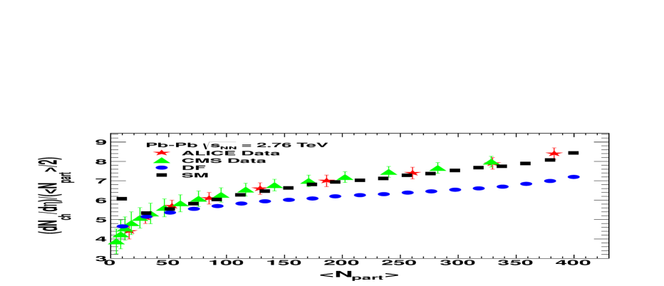
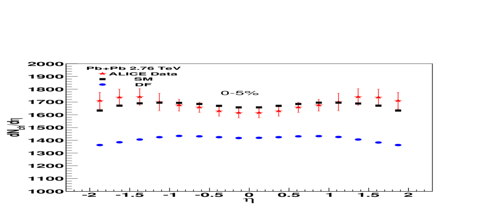
We have generated events, with parameters $a=2.2$, $b=0.5$ $\rm GeV^{-2}$, in the HIJING model for Lund string Fragmentation function as used in ampt:ref1 . Also the values $\mu=1.8$ $\rm fm^{-1}$ and $\alpha_{s}=0.47$, are used for the screening mass in the partonic matter and the strong coupling constant respectively, as used in the AMPT model to describe elliptic flow ampt:alphamu1 ; ampt:alphamu2 and two-pion correlations ampt:alphamu3 . These values for the parameters $a$, $b$, $\mu$ and $\alpha_{s}$ were used in the AMPT for the study of beam energy dependence of anisotropy in the azimuthal distribution ($v_{2}$ and $v_{3}$) of the produced particles  dronika:sumit . Fig. 1 (left) shows the dependence of charged particle density ($dN_{ch}/d\eta$) on the participating nucleons ($N_{part}$) and (right) on the $\eta$ for $0-5\%$ central Pb–Pb collisions. AMPT DF and SM data values are compared with the experimental data from LHC. SM mode of AMPT is observed to be in good agreement with the experimental data. We have generated a total of $23424$ DF and $19669$ SM events with impact parameter $\leq 5$. 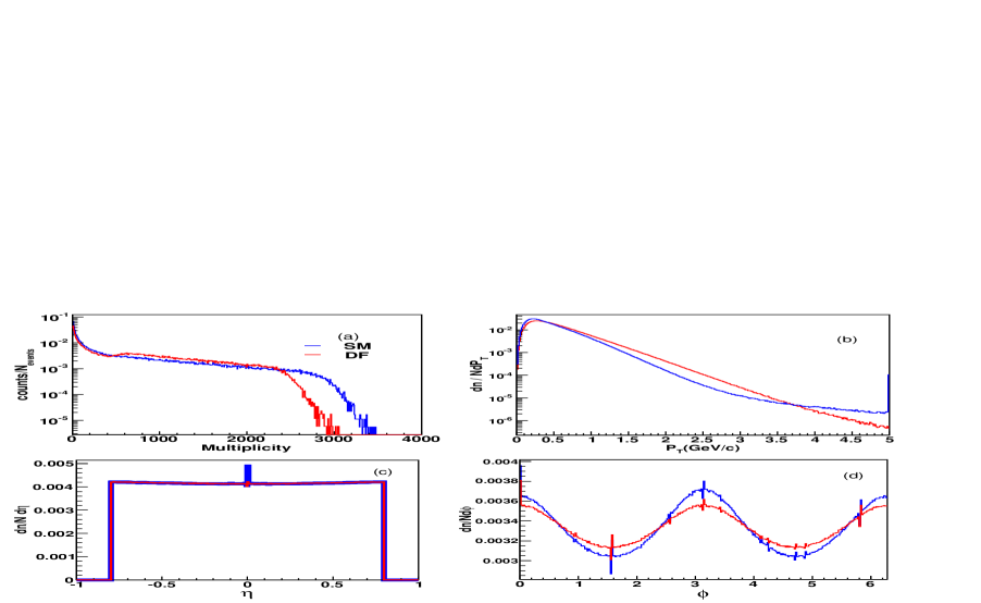For charged particles (pions, kaons and protons) with $|\eta|\leq 0.8$ and full azimuthal coverage in the $p_{\mathrm{T}}$ windows with width $\Delta p_{\mathrm{T}}=0.1$ GeV/c, we have studied their local multiplicity fluctuations. Fig. 2 shows (a) the multiplicity distributions (normalised with the number of events), (b) $p_{\mathrm{T}}$ distributions ($\leq 5$ GeV/c), (c, d) $\eta$ and $\phi$ distributions of the generated data. These $p_{\mathrm{T}}$ bins and respective average charged particle multiplicities are tabulated in Table 1. In those figures we see the differences in the results from the SM and DF settings in AMPT. We note that Ref. [16] shows a good agreement of the $p_{T}$ distribution of the SM version of the AMPT model with that of the LHC data. In the following we move on to observables that have not been analyzed for the LHC data, but we study them first for the simulated data from AMPT.

Figure 4: Average charged particle bin multiplicities in the $p_{\mathrm{T}}$ bins : (a) DF (b) SM AMPT model.

V Results of Analysis

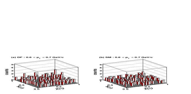
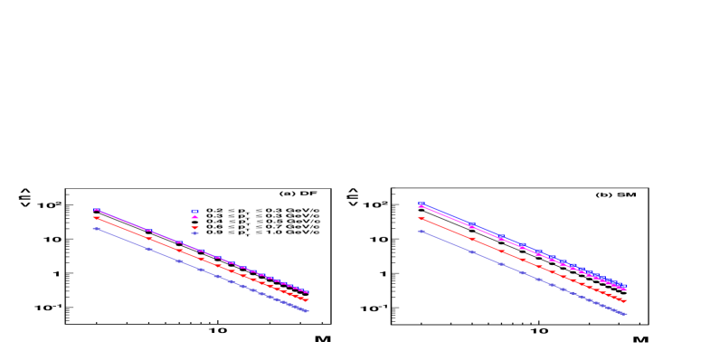
From the $X(\eta)$ and $X(\phi)$ distributions obtained from the $\eta$ and $\phi$, as defined in Eq. (15), we get the $(X(\eta),X(\phi))$ phase space, for each event, which is binned into $M^{2}$ cells with the minimum value of $M$ being $2$ and the maximum value going anywhere between $10$ to $32$. The maximum $M$ value depends on the average bin multiplicity and the order of the moment. Fig. 3 shows a lego plot for some arbitrary DF and SM data event in $0.6\leq p_{\mathrm{T}}\leq 0.7$ $p_{\mathrm{T}}$ bin, of the $(X(\eta),X(\phi))$ phase space, having $M$ = 32. We note that there are no bins with $n>2$. That does not mean that there are no events with larger $n$. What we see in Fig. 3 is that there is no obvious clustering. In Fig. 4 the dependence of the average bin multiplicity ($\langle n\rangle$) on $M$ clearly shows the $1/M^{2}$ decrease in log-log plot in each case of the $p_{T}$ cuts, as it should. The point of exhibiting Fig. 4 is to show how small $\langle n\rangle$ becomes at high $M$. Furthermore, at low $p_{\mathrm{T}}$, $\langle n\rangle$ is smaller for the DF mode compared to the SM, but the relative magnitudes are reversed at higher $p_{\mathrm{T}}$.

Figure 5: Distributions in $F_{q}$ for $0.6\leq p_{\mathrm{T}}\leq 0.7$ GeV/c. (a) q = 2 in DF, (b) q = 4 in DF, (c) q = 2 in SM, (d) q = 4 in SM.

Note that at high $M$, $\langle n\rangle$ becomes less than $0.1$ for $p_{\mathrm{T}}>0.9$ GeV/c in both modes. That means that the ($\eta,\phi$) space is very empty. But how the particles in an event under such conditions are distributed over the whole space can fluctuate greatly. Because of the denominator in Eq. (1), a cluster of particles with multiplicity $n\geq q$ in an event would produce a large value for $F_{q}(M)$ for that event. On the other hand, if the particles are evenly distributed, $F_{q}(M)$ would be smaller. Thus the spatial pattern of the event structure should be revealed in the distribution of $F_{q}(M)$ after collecting all events.

Figure 6: M dependence of $\langle F_{q}\rangle$ in various $p_{\mathrm{T}}$ bins. Solid symbols for DF and open symbols for SM.

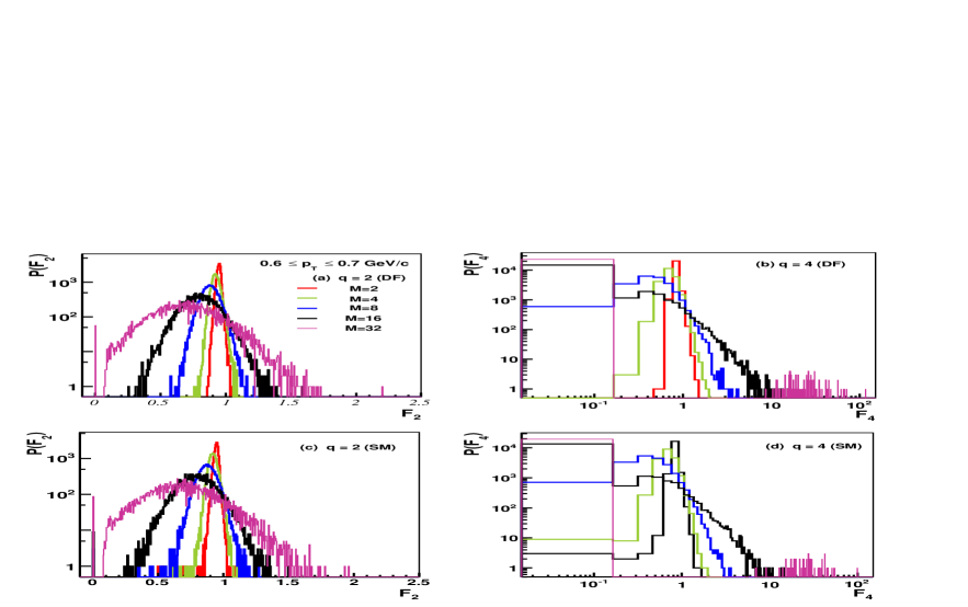
We have determined the $P(F_{q}^{e})$ distributions for each data set for $q=2,3,4,5$ and for different $M$ values. We show the $P(F_{q}^{e})$ distributions in the $p_{\mathrm{T}}$ window $0.6\leq p_{\mathrm{T}}\leq 0.7$ GeV/c in Fig. 5 for $q=2$ in (a) and (c) and for $q=4$ in (b) and (d); the DF and the SM simulated events are in the two rows in the figure. We show only the $M$ values in multiples of 2. Similar distributions are obtained for the other cases also, i.e., for the $q=3$ & $5$ and for all the $p_{\mathrm{T}}$ bins for both modes, but are not exhibited here. It is observed that for $q=2$ in (a) and (c), the distributions $F_{2}$ become wider as $M$ increases; however for $q=4$ in (b) and (d) the $F_{4}$ distributions develop long tails, particularly when $M$ is large. Note the log scale on the horizontal axes. In Fig. 5 (a) and (c), for $q$ = 2, the peaks are moving to the left as $M$ increases, thus decreasing $\left<F_{2}\right>$; however, for $q$ = 4, in Fig. 5 (b) and (d), the upper tails move towards right as $M$ increases, while the lower sides move more and more towards left thereby decreasing the $\langle F_{q}\rangle$. It means that in small bins the average bin multiplicity $\left<n\right>$ [which is also $f_{1}(M)$] is so small that when there is a spike of particles in one such bin with $n\geq 4$, the non-vanishing numerator in Eq. (6) results in a large value for $F^{e}_{q}(M)$ for that $e^{\rm th}$ event. In other words, for low average bin multiplicity and at higher moment-order $q$, there are not many events having $n\geq q$, but when such an event occurs, we have $P(F_{q}^{e})\neq 0$ at a high value of $F_{q}^{e}$. That is the nature of fluctuations in event structure that we look for, as quantified by $P(F_{q}^{e})$. As it turns out (to be discussed below), AMPT does not generate enough fluctuations to exhibit properties of PT.

Figure 7: F-scaling plots of $\langle F_{q}\rangle$ vs $\langle F_{2}\rangle$ for various $p_{\mathrm{T}}$ intervals. Solid symbols for DF and open symbols for SM.

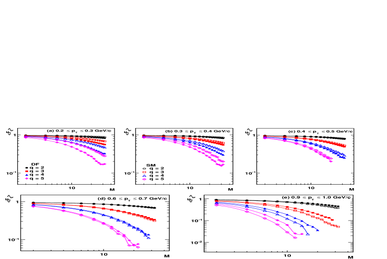
The first moment of $P(F_{q}^{e})$ is $\langle F_{q}^{e}\rangle$, whose dependence on $M$ can be studied in log-log plots as shown in Fig. 6 for various $p_{T}$ cuts. From the plots, it is observed that values of the moments decrease as the bin size decreases or as $M$ value increases. For both the DF and SM in AMPT that relationship between $F_{q}(M)$ and $M$ is inverse of that in the Eq. (3) such that we represent here the intermittency index as $\varphi_{q}^{-}$ instead of with $\varphi_{q}$; that is

$$F_{q}^{\rm AMPT}(M)\propto M^{\varphi^{-}_{q}},\qquad\varphi^{-}_{q}<0.$$ (16)

Figure 8: Log-Log plots of $\beta_{q}$ vs $q-1$ for (a) DF and (b) SM. Errors plotted here are the fitting errors, as obtained from the line fit of the F-scaling plot.

Hence, with negative $\varphi^{-}_{q}$ it is found that the charged particles generated by the Default and the String Melting modes of the AMPT model exhibit inverse of the intermittency behavior, which we term here as negative intermittency. Eq. (16) suggests that $F_{q}^{\rm AMPT}(M)\to 0$ at large $M$ and $q$, implying that the fluctuation is even less than Poissonian. Thus in AMPT there are too few rare high-multiplicity spikes anywhere in phase space. Eq. (16) is a quantification of the phenomenon exemplified by Fig. 3 for one event, and is a mathematical characterization after averaging over many events. This same behavior was generated in hy for the events belonging to the non-critical class.

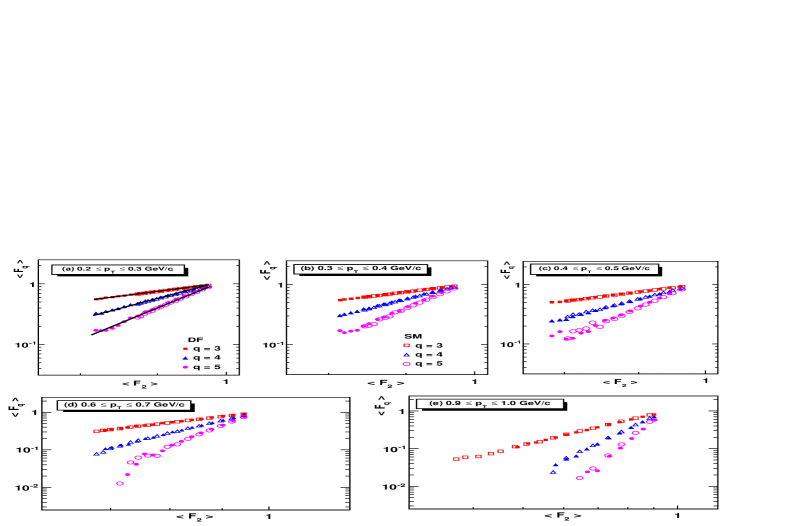
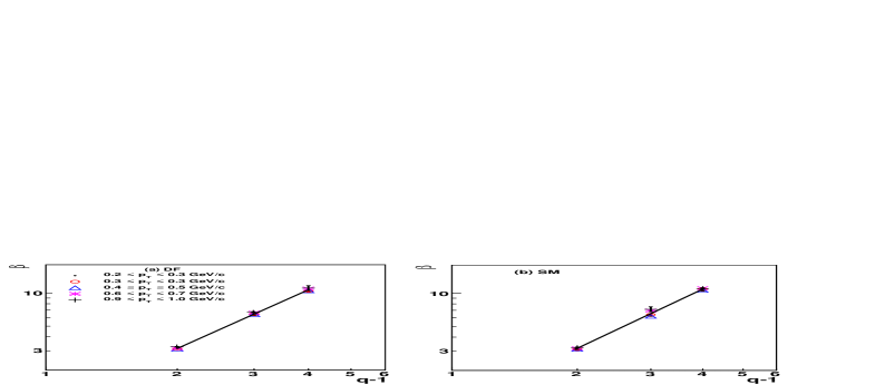
Though, we observe negative intermittency for both DF and SM mode of the AMPT data, it is of interest to check whether there is F-scaling in accordance to Eq. (4). We plot $F_{\mathrm{q}}(M)$ versus $F_{2}(M)$ as is shown in Fig. 7. Evidently, there is remarkable linearity in the log-log plots, thus revealing the absence of any relevant scale. For each set of points linear fit has been performed to determine the value of the slope, $\beta_{q}$, as exemplified by the straight lines in Fig. 7 (a). Thus we obtain a scaling exponent $\nu_{-}$ in

$$\beta_{q}=(q-1)^{\nu_{-}},$$ (17)

similar to that in Eq. (5), but for negative intermittency. The dependence of $\beta_{q}$ on ($q-1$) is shown in Fig. 8, which exhibits good linearity in the log-log plots. The values of $\nu_{-}$ are given in Table 2 for different $p_{\mathrm{T}}$ windows and for both modes of the AMPT model studied here. Those values (which are positive) should not be compared with $\nu=1.304$ in Eq. (5) because $\nu$ is fundamentally different from $\nu_{-}$ on account of the difference between the positivity of $\varphi_{q}$ and the negativity of $\varphi^{-}_{q}$. It is to be noted that the errors on the values are the fitting errors.

$p_{\mathrm{T}}$ window	$\nu_{-}$	$\nu_{-}$
(in GeV/c)	(DF)	(SM)
$0.2\leq p_{\mathrm{T}}\leq 0.3$	$1.738\pm 0.008$	$1.753\pm 0.004$
$0.3\leq p_{\mathrm{T}}\leq 0.4$	$1.774\pm 0.007$	$1.793\pm 0.005$
$0.4\leq p_{\mathrm{T}}\leq 0.5$	$1.758\pm 0.006$	$1.755\pm 0.006$
$0.6\leq p_{\mathrm{T}}\leq 0.7$	$1.824\pm 0.008$	$1.869\pm 0.016$
$0.9\leq p_{\mathrm{T}}\leq 1.0$	$1.778\pm 0.013$	$1.781\pm 0.011$

Table 2: Scaling exponents for negative intermittency in the Default and String Melting modes of the AMPT Model.

Figure 9: $M$ dependence of $C_{p,q}$ for the $p_{\mathrm{T}}$ window $0.6\leq p_{\mathrm{T}}\leq 0.7$ GeV/c in case of DF and SM modes of the AMPT model.

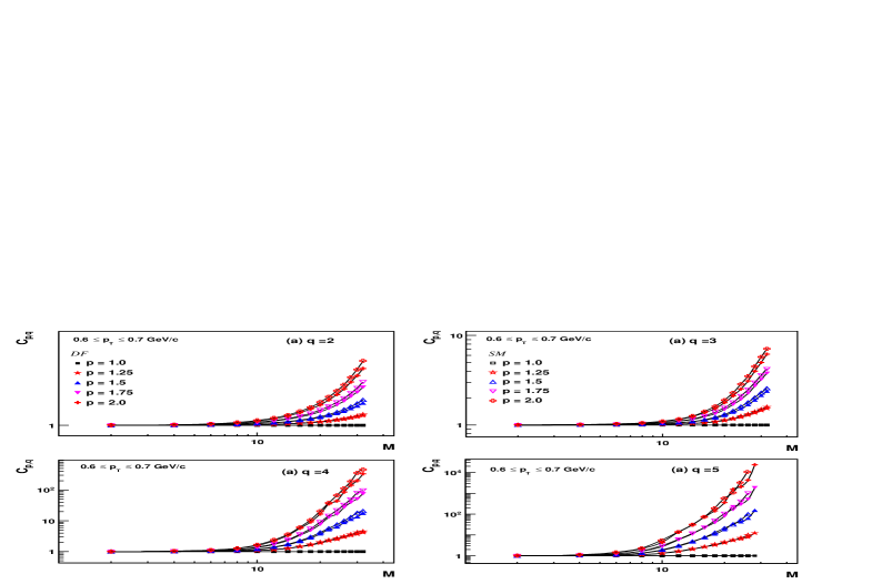
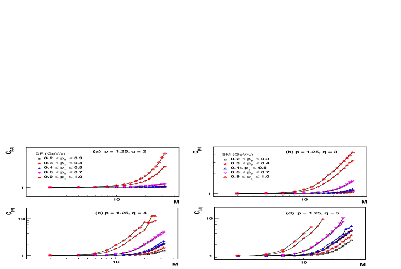
Since large fluctuations result in the high $F_{q}$ tails of $P(F_{q})$, as exemplified in Fig. 5 (b) and (d), it is advantageous to put more weight on the high $F_{q}$ side in averaging over $P(F_{q})$. That is just what the double moment $C_{p,q}(M)$ does. We have determined $C_{p,q}\rm(M)$ for q = 2, 3, 4, 5 and p = 1.0, 1.25, 1.5, 1.75 and 2.0. The number of bins, $M$, takes on values from 2 to the maximum value possible while having reasonable $\langle n_{m}\rangle$ such that $F_{q}^{e}\neq 0$. For example for the $0.9\leq p_{\mathrm{T}}\leq 1.0$ GeV/c window for q = 5, the average bin multiplicity is very small, so we take $M$ maximum to 12 for DF data. To check whether $C_{p,q}\rm(M)$ follows the scaling behavior with $M$, $C_{p,q}$ is plotted against $M$. Fig. 9 (a) to (d) shows respectively, for $q$ = 2, 3, 4 and 5, the $C_{p,q}$ versus $M$ plot in the log-log scale for the window $0.6\leq p_{\mathrm{T}}\leq 0.7$ GeV/c, and for various values of $p$ between 1 and 2. It can be seen that the plots of $C_{p,q}$ versus $M$ have similar shapes for all cases but only with different scales. Further as expected for all values of $q$, for $p$ = 1.0, the $C_{p,q}=1$ . For $p>1.0$, $C_{p,q}$ increases with $M$ and $q$ values. Similar calculations are also done for the other $p_{\mathrm{T}}$ windows as is shown in Fig. 10 (a) to (d) for the case of fixed $p=1.25$ and $q$ = 2, 3, 4, 5 respectively. From the Fig. 9 and 10 we observe that the moment $C_{p,q}$ increases with $M$. Note especially that $C_{p,q}(M)$ in Fig.  10 increases as $p_{T}$ increases. That is due to the fact that at higher $p_{T}$ the window multiplicity is lower so the bin fluctuation must be larger to register larger $F_{q}(M)$.

Figure 10: $M$ dependence of $C_{p,q}$ in different $p_{\mathrm{T}}$ windows for DF and SM AMPT model, for $p=1.25$.

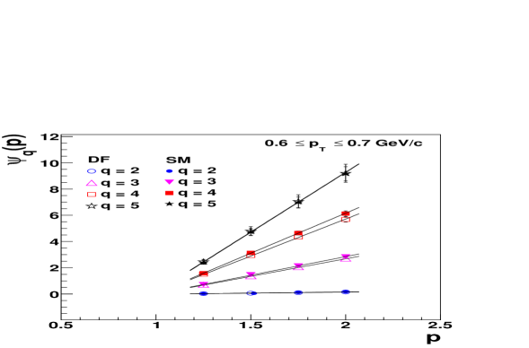
To extract the erraticity behavior we consider the high $M$ region where linear fits are performed for each $q$ and $p$ value so as to determine $\psi_{q}(p)$. We see in Fig. 11 that for $0.6\leq p_{\mathrm{T}}\leq 0.7$  $\psi_{q}(p)$ depends on $p$ linearly for each $q$. Thus the erraticity indices defined in Eq. (14) can be determined. Similar plots are obtained for the other $p_{\mathrm{T}}$ windows also. The values of $\mu_{q}$ with the fitting errors are given in Table 3. It can be seen from the table that as $p_{T}$ value increases (thus decreasing bin multiplicity), the erraticity indices increase for both modes of the AMPT model.

Comparing the $\mu_{q}$ values for the DF and SM data within the same window and for the same values of $q$, it is observed that $\mu_{q}$ has higher values for the DF mode in comparison to SM for the $p_{\mathrm{T}}$ windows below $0.6$ GeV/c, but the values are mixed for $p_{\mathrm{T}}>0.6$ GeV/c. That phenomenon is related to the average multiplicities of the two modes reversing their relative magnitudes at higher $p_{T}$, as pointed earlier in connection to Fig. 4. However it is to be noted from Fig. 11 that the dependence of $\psi_{q}(p)$ on $p$ is distinguishable for the two modes of the AMPT for only $q$ = 4. Coincidentally, as observed in hy , $\mu_{4}$ seems to be a good measure to compare the erraticity indices of the different systems and data sets at these energies.

Figure 11: The $\psi_{q}$ dependence on the $p$ for DF and SM AMPT in the $0.6\leq p_{\mathrm{T}}\leq 0.7$ GeV/c window. The slope of this gives the $\mu_{q}$.

We observe that the values of $\mu_{4}^{DF}$ and $\mu_{4}^{SM}$ for all windows are larger than those obtained for the critical data set in hy , on the same side as the non-critical case. To reflect on the significance of this result, let us point out the difference between erraticity and intermittency. We have found $\varphi^{-}$ to be negative because $P(F_{q})$ broadens, as $M$ increases, with the average $\left<F_{q}\right>$ shifting to the lower region of $F_{q}$, thus resulting in negative intermittency. We did notice that the upper tails move to the right, suggesting the presence of some degree of clustering. To emphasize that part of $P(F_{q})$ we have taken higher $p$-power moments of $\phi_{q}(M)$, which suppress the lower side of $F_{q}$ while boosting the upper side. The scaling properties of $C_{p,q}(M)$ therefore deemphasize what leads to negative intermittency. Thus the erraticity indices $\mu_{q}$ reveal a different aspect of the fluctuation patterns than the scaling indices $\nu^{-}$. Perhaps they are influenced by the production of jets which show up as clusters, although high-$p_{T}$ jets are towers in the lego plots in $\eta$-$\phi$ with large $p_{T}$, while we make low $p_{T}$ cuts. Details of that aspect of physics require special focused investigation to be done elsewhere. Our study here has revealed interesting properties of scale-invariant fluctuations that should be compared to the real data. Since AMPT contains no dynamics of collective behavior, we should not expect $\nu^{-}$ and $\mu_{q}$ to exhibit properties of phase transition.

VI Summary

We have studied the local multiplicity fluctuations in the spatial patterns of charged particles and their event-by-event fluctuations, in central events generated by the Default and the String Melting modes of the AMPT model, using the intermittency and erraticity analysis methodology. We find that the factorial moments decrease with increasing bin numbers, contrary to the usual properties of intermittency observed at lower energies. It means that events with localization of even moderate multiplicities in small bins at low $p_{T}$ are not generated by AMPT. That is not the property of critical phenomenon, which is supposed to generate fluctuations of all cluster sizes. Since the dynamics of collective behavior is not built into AMPT, no phase transition of the GL type or critical behavior discussed in Ref. [22] is expected. The erraticity analysis that we have performed shed further light on the nature of fluctuations, showing that the system generated by AMPT is not near criticality. The scaling exponent $\nu^{-}$ and $\mu_{q}$ that we have determined are useful quantification of our results so that they can be used effectively to compare with other models irrespective of the issues about phase transition. Lastly, the experience that we have gained in this study is extremely beneficial for our analysis of the real data collected at LHC.

VII Acknowledgements

We are thankful to Dr. R.C. Hwa for the very useful discussions and continuous guidance during the analysis of this work. His patience to discuss and timely response to various queries throughout are really appreciated. We are thankful to Prof. S.K. Badyal, Dr. Y.P. Viyogi for the motivation and guidance. We are also thankful to Dr. Tapan K. Nayak and Dr. Premmoy Ghosh of VECC, Kolkata, Dr. Shakeel Ahmad of AMU, Aligarh and Prof. Anju Bhasin of University of Jammu for their inputs on various analysis related details from time to time. We acknowledge the services provided by the grid computing facility at VECC-Kolkata, India for facilitating to perform a part of the computation used in this work.

q	$0.2\leq p_{T}\leq 0.3$	$0.3\leq p_{T}\leq 0.4$	$0.4\leq p_{\mathrm{T}}\leq 0.5$	$0.6\leq p_{\mathrm{T}}\leq 0.7$	$0.9\leq p_{\mathrm{T}}\leq 1.0$
			(in GeV/c)
DF
2	$0.043\pm 0.002$	$0.045\pm 0.002$	$0.062\pm 0.003$	$0.154\pm 0.008$	$0.739\pm 0.043$
3	$0.901\pm 0.081$	$0.940\pm 0.081$	$1.304\pm 0.118$	$2.678\pm 0.155$	$4.502\pm 0.147$
4	$4.325\pm 0.243$	$4.532\pm 0.234$	$5.478\pm 0.258$	$5.640\pm 0.203$	$7.484\pm 0.361$
5	$6.202\pm 0.302$	$6.150\pm 0.175$	$7.396\pm 0.437$	$9.107\pm 0.693$	$8.643\pm 0.537$
SM
2	$0.016\pm 0.001$	$0.027\pm 0.001$	$0.048\pm 0.002$	$0.174\pm 0.011$	$1.014\pm 0.064$
3	$0.328\pm 0.025$	$0.531\pm 0.043$	$1.019\pm 0.077$	$2.832\pm 0.137$	$4.960\pm 0.150$
4	$2.481\pm 0.183$	$3.385\pm 0.235$	$3.935\pm 0.021$	$6.101\pm 0.214$	$7.359\pm 0.305$
5	$5.143\pm 0.022$	$5.745\pm 0.312$	$6.159\pm 0.280$	$8.360\pm 0.533$	$7.655\pm 0.358$

Table 3: Erraticity index in DF and SM modes of the AMPT Model

References

- (1) I. Arsene et.al., Nucl. Phys. A 757, 1 (2005).
- (2) B.B. Back et. al., Nucl. Phys. A 757, 28 (2005).
- (3) J. Adams et. al., Nucl. Phys. A 757, 102 (2005).
- (4) K. Adcox et. al., Nucl. Phys. A 757 184, (2005).
- (5) J. Schukraft for ALICE Collaboration, J. Phys. G 124003, (2011).
- (6) B. Wyslouch for the CMS Collaboration, J. Phys. G 38, 124005 (2011).
- (7) M. Gyulassy and L. McLerran, Nucl. Phys. A 750, 30 (2005).
- (8) E.V. Shuryak, Nucl. Phys. A 750, 64 (2005).
- (9) Heiselberg Phys. Rep. 351, 161 (2001).
- (10) E.A. DeWolf, I.M. Dremin and W. Kittle, Phys. Rep. 270,1 (1996), I.G. Knowler and G.D. Lafferty, J. Phys. G 23, 73(1997).
- (11) P. Bozek, M. Plozajezak and R. Botet Phys. Rep. 252, 101 (1995).
- (12) Z.W. Lin, S. Pal, C.M. Ko, B.A. Li & B. Zhang, Phys. Rev. C 64, 011902 (2001);
- (13) Z.W. Lin, S. Pal, C.M. Ko, B.A. Li & B. Zhang, Nucl. Phys. A 698, 375 (2002).
- (14) B. Zhang, C.M. Ko, B.A. Li, Z.W. Lin and B.H. Sa Phys. Rev. C 62, 054905 (2000).
- (15) S. Pal, C.M. Ko and Z.W. Lin Nucl. Phys. A 730, 143 (2004).
- (16) Jun Xu and Che Ming Ko, Phys. Rev C 83, 034904 (2011).
- (17) Jun Xu and Che Ming Ko, Phys. Rev C 84, 014903 (2011).
- (18) Jun Xu and Che Ming Ko, Phys. Rev C 84, 044907 (2011).
- (19) G.-L. Ma, Phys. Lett. B 724, 278 (2013).
- (20) A. Bialas and R. Peschanski, Nucl. Phys. B 273, 703 (1986); B 308, 867 (1988).
- (21) W. Kittle and E.A. De Wolf, Soft Multihadron Dynamics (World Scientific, Singapore 2005), p. 429.
- (22) A. Bialas and R.C. Hwa, Phys. Lett. B 253, 436 (1991).
- (23) R.C. Hwa and M.T. Nazirov, Phys. Rev. Lett. 69, 741 (1992).
- (24) R.C. Hwa, Phys. Rev. D 47, 2773 (1993). R.C. Hwa, “Scaling Properties of Quark-Hadron Phase Transition” in Quark-Gluon Plasma 2, edited by R.C. Hwa (World Scientific, Singapore, 1995).
- (25) M.R. Young, Y. Qu, S. Singh and R.C. Hwa, Opt. Commun. 105, 325 (1994).
- (26) Z. Cao, Y. Gao and R.C. Hwa, Z. Phys. C 72, 661 (1996).
- (27) Z. Cao, R. Hwa, Phys. Rev. Lett. 75, 1268 (1995), Phys. Rev. D 53, 6608 (1996); Phys. Rev D 54, 6674 (1996).
- (28) R.C. Hwa and C.B. Yang, Phys. Rev. C 85,044914(2012).
- (29) W. Ochs, Z Phys. C 50, 339 (1991).
- (30) Z. Cao and R.C. Hwa, Phys. Rev. D 61, 074011(2000).
- (31) B. Zhang, C.M. Ko, B.A. Li & Z.W. Lin, Phys. Rev. C 61, 067901 (2000).
- (32) Z. W. Lin, C.M. Ko, B.A. Li, B. Zhang and S. Pal Phys. Rev. C 72, 064901 (2005).
- (33) B. Zhang, C.M. Ko, B.A. Li, Z.W. Li & S. Pal Phys. Rev. C 65, 054909 (2002).
- (34) C.M. Ko, Z.W. Lin and S. Pal, Heavy Ion Physics 17, 219 (2003).
- (35) X.N. Wang and M. Gyulassy, Phys Rev. D 44, 3501 (1991).
- (36) B. Zhang, Comput. Phys. Comm. 109, 193 (1998).
- (37) B.A. Li and C.M. Ko, Phys. Rev. C 52, 2037 (1995).
- (38) Z.W. Lin and C.M. Ko, Phys. Rev. C 65, 034904 (2002).
- (39) L.W. Chen, C.M. Ko, and Z.W. Lin, Phys. Rev. C 69, 031901(R) (2004).
- (40) Z.W. Lin, C.M. Ko, and S. Pal, Phys. Rev. Lett. 89, 152301 (2002).
- (41) Dronika Solanki, Paul Sorensen, Sumit Basu, Rashmi Raniwala and Tapan Kumar Nayak, Phys. Lett. B 720, 352-357 (2013).
- (42) K. Aamodt et. al. (ALICE Collaboration), Phys. Rev. Lett. 106, 032301 (2011).
- (43) S. Chatrchyan et. al. (CMS Collaboration), JHEP 08 141, (2011).
- (44) E. Abbas et. al. (ALICE Collaboration), Phys. Lett. B 726, 610-622 (2013).