Many-body microhydrodynamics of colloidal particles with active boundary layers

Abstract

Colloidal particles with active boundary layers - regions surrounding the particles where non-equilibrium processes produce large velocity gradients - are common in many physical, chemical and biological contexts. The velocity or stress at the edge of the boundary layer determines the exterior fluid flow and, hence, the many-body interparticle hydrodynamic interaction. Here, we present a method to compute the many-body hydrodynamic interaction between $N$ spherical active particles induced by their exterior microhydrodynamic flow. First, we use a boundary integral representation of the Stokes equation to eliminate bulk fluid degrees of freedom. Then, we expand the boundary velocities and tractions of the integral representation in an infinite-dimensional basis of tensorial spherical harmonics and, on enforcing boundary conditions in a weak sense on the surface of each particle, obtain a system of linear algebraic equations for the unknown expansion coefficients. The truncation of the infinite series, fixed by the degree of accuracy required, yields a finite linear system that can be solved accurately and efficiently by iterative methods. The solution linearly relates the unknown rigid body motion to the known values of the expansion coefficients, motivating the introduction of propulsion matrices. These matrices completely characterize hydrodynamic interactions in active suspensions just as mobility matrices completely characterize hydrodynamic interactions in passive suspensions. The reduction in the dimensionality of the problem, from a three-dimensional partial differential equation to a two-dimensional integral equation, allows for dynamic simulations of hundreds of thousands of active particles on multi-core computational architectures. In our simulation of $10^{4}$ active colloidal particle in a harmonic trap, we find that the necessary and sufficient ingredients to obtain steady-state convective currents, the so-called “self-assembled pump”, are (a) one-body self-propulsion and (b) two-body rotation from the vorticity of the Stokeslet induced in the trap.

I Introduction

There are many examples in physics, chemistry and biology, where non-equilibrium processes at the surface of a particle drive exterior fluid flow and lead, possibly, to motion of the particle. Such non-equilibrium processes are frequently confined to a thin region surrounding the particle, as for example in phoretic phenomena anderson1989colloid , motion in chemically reacting flows paxton2006chemical , and in ciliary propulsion blake1971a . Following the pioneering efforts of Helmholtz helmholtz1879studien , Smoluchowski smoluchowski1903 and Derjaguin derjaguin1947kinetic , methods have been developed, to relate the rigid body motion of a particle to the structure of the active boundary layer that surrounds it anderson1989colloid . The corresponding many-body problem, of determining the collective motion and exterior flow of $N$ particles with active boundary layers, has received much less attention anderson1981concentration ; chen1988electrophoresis ; rider1993dynamic .

In this paper, we present a systematic method of computing many-body hydrodynamic interactions between colloidal particles due to the exterior microhydrodynamic flow produced by active boundary layers at their surfaces. The hydrodynamic interaction between particles is mediated by the ambient fluid which, in the microhydrodynamic limit, obeys Stokes equation. The boundary conditions are determined by the flow in the active boundary layer. Depending on the structure of the boundary layer, these may be Dirichlet conditions specifying the active surface velocity, or, Neumann conditions specifying the surface traction. In either case, the fluid flow in the bulk admits an integral representation in terms of the velocities and tractions on the particle boundaries. We use the integral representation to derive the rigid body motion of the particles, in terms of the boundary conditions and any external forces and torques that may be applied to the particles.

In section II we present the Galerkin method of solving the boundary integral equation. In this method, the boundary tractions and velocities are expanded in an infinite-dimensional basis of complete, orthogonal functions defined on the particle boundaries. On enforcing the boundary condition to this bulk fluid velocity, an integral equation is obtained for the unknown boundary traction (when Dirichlet conditions are specified) or the unknown boundary velocities (when Neumann conditions are specified). The solution of this boundary integral equation provides both the particle velocities and angular velocities and the bulk fluid flow. On enforcing the boundary conditions in a weighted residual sense, with weighting functions that are identical to the expansion functions, a system of linear equations is obtained for the unknown expansion coefficients. The solution of the linear system determines the expansion coefficients of the unknown boundary traction (when Dirichlet conditions are specified) or that of the unknown boundary velocities (when Neumann conditions are specified). We focus attention on the former situation, where the velocity profile in the boundary layer is provided. The velocity seen by the exterior fluid is the sum of the rigid body motion of the particle and the velocity at the outer edge of the boundary layer. When the boundary layer is thin compared to the size of the particle, the boundary condition can be applied directly on the surface of the particle as the sum of a rigid body motion and an active slip. The problem is solved when the rigid body motion and the exterior fluid flow are determined completely in terms of the slip velocities specified on each particle surface. As the Stokes equations are linear, the rigid body motion must be a linear functional of the active slip. We show how this linear functional relationship is expressed through propulsion matrices, which appear naturally in the solution of linear system of equations. The propulsion matrices relate the vector of rigid body motions of the particle to the vector of expansion coefficients of the active slip. The problem of computing hydrodynamic interactions between active colloidal particles is, thereby, reduced to that of computing the propulsion matrices. The analysis also reveals that the propulsion matrices are a sum of two parts : one is the contribution from the superposition of flows due to each particle and the other is a correction required to satisfy the boundary conditions. The first is the two-body contribution to hydrodynamic interactions while the second contains the genuine many-body contribution.

In section III, which contains the central results of this paper, we focus on spherical colloidal particles with active slip. We chose tensorial spherical harmonics as the Galerkin expansion basis, which are complete and orthogonal on the surface of the sphere. The simplicity of the spherical shape allows us to calculate all boundary integrals and matrix elements analytically, in terms of derivatives of the Green’s function of Stokes flow. The structure of the flow has a pleasing simplicity, as shown in Table 2. At any order, there are at most three kinds of derivatives, which are the irreducible gradient of the Green’s function, its curl and its Laplacian. This leads to a simple classification of the flow in terms of irreducible tensors of increasing rank. As numerical quadrature is no longer necessary to evaluate the matrix elements, the linear system can be solved both efficiently and accurately. This linear solution yields the mobility and propulsion matrices which completely describe the many-body hydrodynamic interactions in active suspensions.

In section IV we truncate the infinite series expansion of the boundary fields to the minimal number of terms required to produce active translations and rotations. At this order of truncation, all long-ranged hydrodynamic interactions are also automatically included. We show that there are exactly two coefficients in the expansion of the active slip that produce translation and rotation. The translational coefficient produces a flow that decays inverse cubically with distance while the rotational coefficient produces a flow that decays inverse quartically with distance. We plot the flows generated by all terms in the truncated expansion in figure 2.

In section V we illustrate our general formalism with a detailed study of the dynamics of active colloidal particles in a harmonic trap. For the squirming motion of a sphere, we recast the leading terms of Lighthill lighthill1952 and Blake’s blake1971a solution in our formalism. The problem of squirmers in a harmonic potential has been studied earlier by Nash et al. nash2010 , and more recently, by Hennes, Wolff and Stark hennes2014self . In our study, we attempt to find out the necessary and sufficient ingredients to obtain steady-state convective currents, the so-called “self-assembled pump”. We find that the key ingredients necessary for the pumping state are (a) one-body self-propulsion and (b) two-body rotation from the vorticity of the Stokeslet induced in the trap. Thus, neither tumbling (as included in Nash et al.) nor stresslet flows (as included in Hennes et al.) are necessary. Our simulation of $10^{4}$ squirmers, the largest such simulation till date, displays the formation of the self-assembled pump with greater clarity than previous studies.

We conclude with a comparison of our approach with existing theories of collective hydrodynamics of active particles and with a discussion of applications of the integral equation technique to rheology in active colloidal suspensions.

II Boundary integral equation for microhydrodynamics

We consider $N$ active particles, of arbitrary shape, in an incompressible fluid of viscosity $\eta$. The position of the center of mass, the translational velocity and the rotational velocity about the center of the mass are $\mathbf{R}_{n}$, $\mathbf{V}_{n}$ and $\mathbf{\Omega}_{n}$ respectively. Points on the particle boundary $S_{n}$ are labelled, in the frame attached to the center of the mass, by $\bm{\rho}_{n}$, or equivalently, in the laboratory frame by $\mathbf{r}_{n}=\mathbf{R}_{n}+\bm{\rho}_{n}$. Particle trajectories are obtained from Newton’s equations, where the right hand sides include both contact and body contributions,

$$M\ \dot{\mathbf{V}}_{n}=\mathbf{F}_{n}+\mathbf{F}_{n}^{\mathrm{e}},\qquad I\ \dot{\mathbf{\Omega}}_{n}=\mathbf{T}_{n}+\mathbf{T}_{n}^{\mathrm{e}}.$$ (1)

The stress $\bm{\sigma}$ of the ambient fluid provides the surface traction $\mathbf{n}\cdot\bm{\sigma}_{n}$ on each particle, from which the net contact force $\mathbf{F}_{n}=\int\mathbf{n}\cdot\bm{\sigma}_{n}\,\mathrm{d}S_{n}$ and the net contact torque $\mathbf{T}_{n}=\int\bm{\rho_{n}}\times(\mathbf{n}\cdot\bm{\sigma}_{n})\,\mathrm{d}S_{n}$ can be computed. Here $\mathbf{n}$ is the unit normal pointing away from the particle into the fluid, $M$ and $I$ are the mass and the moment of inertia of the particle respectively, and $\mathbf{F}^{e}$ and $\mathbf{T}^{e}$ are external body forces and torques. In the absence of inertia, as appropriate to the microhydrodynamic regime, Newton’s equations reduce to a pair of constraints,

$$\mathbf{F}_{n}+\mathbf{F}_{n}^{\mathrm{e}}=0,\qquad\mathbf{T}_{n}+\mathbf{T}_{n}^{\mathrm{e}}=0.$$ (2)

There is an instantaneous balance between contact and body forces at all times, which precludes any acceleration of the particles. In the absence of external forces, Newton’s equations reduce further to

$$\mathbf{F}_{n}=0,\qquad\mathbf{T}_{n}=0.$$ (3)

The trivial solution to this is $\bm{\sigma}=0$, that is, there is no motion in the absence of external forces and torques. The non-trivial solutions describe active motion, in which translation and rotation are possible in the absence of external forces and torques. It is these non-trivial solutions that we seek here. The velocity and angular velocity, having being determined from non-trivial solutions of the stress, determine the evolution of the positions and orientations through the kinematical equations,

$$\dot{\mathbf{R}}_{n}=\mathbf{V}_{n},\quad\dot{\mathbf{p}}_{n}=\bm{\Omega}_{n}\times{\mathbf{p}}_{n},$$ (4)

where ${\mathbf{p}}_{n}$ is a fixed axis passing through the center of mass of the body. If the shape is not a figure of revolution about this axis, two additional evolution equations, which together describe the motion of the orthogonal triad attached to the center of mass, are necessary.

The contact forces on the particles are determined from the state of flow in the ambient fluid. In the region bounded by the particles, the fluid satisfies Stokes equation landau1987fluid ; batchelor2000introduction ,

$$\bm{\nabla}\cdot\mathbf{v}=0,\quad\bm{\nabla}\cdot\bm{\sigma}=0,$$ (5a)

$$\bm{\sigma}=-p\mathbb{I}+\eta\left(\bm{\nabla}\mathbf{v}+\bm{\nabla}\mathbf{v}^{\mathrm{T}}\right),$$ (5b)

where $\mathbf{v}$, $p$ and $\bm{\sigma}$ are the fluid velocity, pressure and stress respectively. The solution of this equation, with the appropriate boundary conditions, provides the surface traction and hence the contact forces and torques that determine the rigid body motion.

As discussed in the Introduction, a generic consequence of activity on the surface of rigid bodies is the appearance of a boundary layer. When the boundary layer is thin compared to the particle size, its effect appears as a boundary condition, on either the velocity or the traction, at the particle surface. A detailed discussion of both forms of boundary conditions and their applicability to different boundary layer problems is available in anderson1989colloid .

The problem of determining the surface traction is substantially simplified by recognising that the solution of the three-dimensional partial differential equation in (5) can be expressed as an integral of the velocity and traction fields over the boundaries of the particles fkg1930bandwertaufgaben ; ladyzhenskaya1969 ; pozrikidis1992 ; kim2005

$$8\pi\eta\,v_{i}(\mathbf{r}) =-\sum_{m=1}^{N}\int\left[G_{ij}(\mathbf{r},\mathbf{r}_{m})f_{j}(\mathbf{r}_{m})-\eta\,K_{jik}(\mathbf{r},\mathbf{r}_{m})n_{k}v_{j}(\mathbf{r}_{m})\right]\,\mathrm{d}S_{m},\quad\begin{subarray}{c}\displaystyle\mathbf{r}\in V\\ \\ \displaystyle\quad\,\mathbf{r}_{m}\in S_{m}\end{subarray}$$ (6)

$$\nabla_{j}G_{ij}(\mathbf{r},\mathbf{r}^{\prime})=0,$$ (7a)

$$-\nabla_{i}p_{j}(\mathbf{r},\mathbf{r}^{\prime})+\nabla^{2}G_{ij}(\mathbf{r},\mathbf{r}^{\prime})=-\delta\left(\mathbf{r}-\mathbf{r}^{\prime}\right)\delta_{ij},$$ (7b)

$$K_{ijk}(\mathbf{r},\mathbf{r}^{\prime})=-\delta_{ik}\,p_{j}+\nabla_{k}G_{ij}+\nabla_{i}G_{kj}.$$ (7c)

Here $\bm{\rho}=\mathbf{r}-\mathbf{r}^{\prime}$ and $\mathbf{f}(\mathbf{r}_{m})=\mathbf{n}\cdot\bm{\sigma}$ and $\mathbf{v}(\mathbf{r}_{m})$ are, respectively, the traction and velocity on the boundary of the $m$-th particle. $\mathbf{G}(\mathbf{r},\mathbf{r}^{\prime})$ is a Green’s function of Stokes flow, $\mathbf{p}$ is the corresponding pressure vector and $\mathbf{K}(\mathbf{r},\mathbf{r}^{\prime})$ is the stress tensor associated with this Green’s function. The contribution from the boundary which encloses both the fluid and the particles is not included here, since it is assumed that both the Green’s function and the flow vanish on this boundary.

Equating the expression for the bulk fluid velocity to the boundary condition and evaluating the second integral as a principal value leads to an integral equation on the particle boundaries fkg1930bandwertaufgaben ; ladyzhenskaya1969 ; pozrikidis1992 ; kim2005 ,

$$4\pi\eta\,v_{i}(\mathbf{r}_{n}) =-\sum_{m=1}^{N}\int\left[G_{ij}(\mathbf{r}_{n},\mathbf{r}^{\prime}_{m})f_{j}(\mathbf{r}^{\prime}_{m})-\eta\,K_{jik}(\mathbf{r}_{n},\mathbf{r}^{\prime}_{m})n_{k}v_{j}(\mathbf{r}^{\prime}_{m})\right]\,\mathrm{d}S_{m},\quad\begin{subarray}{c}\displaystyle\mathbf{r}_{n}\in S_{n}\\ \\ \displaystyle\,\,\mathbf{r}^{\prime}_{m}\in S_{m}\end{subarray}.$$ (8)

For Dirichlet boundary conditions, this is a self-adjoint Fredholm integral equation of the first kind for the unknown boundary tractions. For Neumann boundary conditions, this is a self-adjoint Fredholm integral equation of the second kind for the unknown boundary velocities. In both cases, the solution linearly relates the surface traction to the surface velocity and the balance of contact and body forces then determines the rigid body motion. The problem of determining the traction is thus reduced to solving a two-dimensional integral equation on the boundaries of the domain instead of a three-dimensional partial differential equation in the bulk.

Here we use the Galerkin method to discretize and solve the boundary integral equation. In this method, the boundary fields are expanded in a complete, orthogonal basis of functions $\phi^{(l)}(\bm{\rho}_{n})$,

$$\mathbf{f}(\mathbf{R}_{n}+\bm{\rho}_{n}) =\sum_{l=0}^{\infty}\mathbf{F}_{n}^{(l)}{\phi}^{(l)}(\bm{\rho}_{n}),$$ (9a)

$$\mathbf{v}(\mathbf{R}_{n}+\bm{\rho}_{n}) =\sum_{l=0}^{\infty}\mathbf{V}_{n}^{(l)}{\phi}^{(l)}(\bm{\rho}_{n}).$$ (9b)

The coefficients corresponding to the constant function and the antisymmetric linear function are, respectively, the force and torque in the traction expansion and the velocity and angular velocity in the velocity expansion. Inserting this in the boundary integral representation, (6), provides an expression for the bulk flow

$$8\pi\eta\,\mathbf{v}(\mathbf{r}) =-\sum_{m=1}^{N}\sum_{l=0}^{\infty}\left[\bm{G}^{(l)}(\mathbf{r},\,\mathbf{R}_{m})\cdot\mathbf{F}_{m}^{(l)}-\eta\bm{K}^{(l)}(\mathbf{r},\,\mathbf{R}_{m})\cdot\mathbf{V}_{m}^{(l)}\right],$$ (10)

in terms of the coefficients of each surface mode $\phi^{(l)}(\bm{\rho}_{m})$ of the velocity and traction fields and the two boundary integrals

$$\bm{G}^{(l)}(\mathbf{r},\,\mathbf{R}_{m}) =\int\mathbf{G}(\mathbf{r},\mathbf{R}_{m}+\bm{\rho}_{m})\,{\phi}^{(l)}(\bm{\rho}_{m})\,\mathrm{d}S_{m},$$ (11a)

$$\bm{K}^{(l)}(\mathbf{r},\,\mathbf{R}_{m}) =\int\mathbf{K}(\mathbf{r},\mathbf{R}_{m}+\bm{\rho}_{m})\cdot\mathbf{n}\,\,{\phi}^{(l)}(\bm{\rho}_{m})\,\mathrm{d}S_{m}.$$ (11b)

To determine the traction coefficients in terms of the velocity coefficients (or vice versa) we insert the velocity and traction expansions in the boundary integral equation, (8), multiply by the $l$-th basis function and integrate both sides over the $n$-th boundary.The boundary conditions are thus enforced in a weighted integral, or weak, sense and not point wise. The expansion and weighting basis functions are chosen to be identical. This Galerkin procedure yields an infinite dimensional system of linear equations which relate the velocity and traction coefficients

$$4\pi\eta\,\mathbf{V}_{n}^{(l)} =-\sum_{m=1}^{N}\sum_{l^{\prime}=0}^{\infty}\left[\bm{G}_{nm}^{(l,\,l^{\prime})}(\mathbf{R}_{n},\,\mathbf{R}_{m})\cdot\mathbf{F}_{m}^{(l^{\prime})}-\eta\bm{K}_{nm}^{(l,\,l^{\prime})}(\mathbf{R}_{n},\,\mathbf{R}_{m})\cdot\mathbf{V}_{m}^{(l^{\prime})}\right].$$ (12)

The matrix elements of this linear system are integrals of the Green’s function and the stress tensor over pairs of boundaries, weighted by the basis functions on each boundary,

$$\bm{G}_{nm}^{(l,\,l^{\prime})}(\mathbf{R}_{n},\,\mathbf{R}_{m}) =\int\int{\phi}^{(l)}(\bm{\rho}_{n})\,\mathbf{G}(\mathbf{R}_{n}+\bm{\rho}_{n},\mathbf{R}_{m}+\bm{\rho}^{\prime}_{m})\,{\phi}^{(l^{\prime})}(\bm{\rho}^{\prime}_{m})\,\mathrm{d}S_{m}\mathrm{d}S_{n},$$ (13a)

$$\bm{K}_{nm}^{(l,\,l^{\prime})}(\mathbf{R}_{n},\,\mathbf{R}_{m}) =\int\int{\phi}^{(l)}(\bm{\rho}_{n})\,\mathbf{K}(\mathbf{R}_{n}+\bm{\rho}_{n},\mathbf{R}_{m}+\bm{\rho}^{\prime}_{m})\cdot\mathbf{n}\,\,{\phi}^{(l^{\prime})}(\bm{\rho}^{\prime}_{m})\,\mathrm{d}S_{m}\mathrm{d}S_{n}.$$ (13b)

This linear system is valid for any shape of particle, any geometry of the enclosing boundary and for both Neumann and Dirichlet boundary conditions.

For concreteness, we shall focus on Dirichlet boundary conditions in the remaining part of this paper. In this case, the velocity seen by the fluid at the outer edge of the boundary layer is the sum of the rigid body motion of the particle and the asymptotic value, $\mathbf{v}^{a}$, of the velocity in the boundary layer,

$$\mathbf{v}({\mathbf{r}})={\mathbf{V}}_{n}+\bm{\Omega}_{n}\times{\bm{\rho}}_{n}+{\mathbf{v}}^{a}({\bm{\rho}}_{n}), \quad{\mathbf{r}}={\mathbf{R}}_{n}+{\bm{\rho}}_{n}\in S_{n},$$ (14a)

$$\int\mathbf{v}\cdot\mathbf{n}\,\mathrm{d}S_{n}=0.$$ (14b)

Here, the active velocity $\mathbf{v}^{a}$ is assumed given while the rigid body motion, $\mathbf{V}$ and $\mathbf{\Omega}$, is to be determined for all $N$ particles. The only constraint we place on the active velocity is that it conserves mass, as reflected in the integral condition of (14b). This makes our theory completely general. In specific cases, the active velocity may be determined by other local fields like the temperature (in thermophoresis), ionic species (in electrophoresis) and chemical species (in diffusiophoresis). Here we assume that any non-fluid degree of freedom necessary to specify the active velocity has already been determined, and thus, our work treats the purely hydrodynamic aspect of the problem.

The structure of the linear system for the Dirichlet problem can be better understood by clearly separating the known quantities from the unknown quantities in (12). In the velocity expansion, the velocity and angular velocity are unknowns, while all remaining coefficients are fixed by the active velocity. In the traction expansion, the contact force and contact torque are determined from Newton’s equations and are, therefore, known quantities, while all remaining coefficients are unknowns. Therefore, we seek to obtain the unknown velocity and angular velocity in terms of the active velocity, constrained by the balance of contact and external forces as required by Newton’s equation.

To the above end, we group the expansion coefficients for all particles into vectors and separate them into “lower” and “higher” vectors

$$\mathsf{V}^{\mathrm{L}} =\left(\mathbf{V}_{1}-\mathbf{V}_{1}^{a},\ldots,\mathbf{V}_{N}-\mathbf{V}_{N}^{a},\,\mathbf{\Omega}_{1}-\mathbf{\Omega}_{1}^{a},\ldots,\mathbf{\Omega}_{N}-\mathbf{\Omega}_{N}^{a}\right)^{T},$$ (15a)

$$\mathsf{V}^{\mathrm{H}} =\left(\cdots,\mathbf{V}^{(l)}_{1},\ldots,\mathbf{V}^{(l)}_{N},\ldots\right)^{T},\qquad\not\in\mathbf{V},\,\mathbf{\Omega},$$ (15b)

$$\mathsf{F}^{\mathrm{L}} =\left(\mathbf{F}_{1},\ldots,\mathbf{F}_{N},\,\mathbf{T}_{1},\ldots,\mathbf{T}_{N}\right)^{T},$$ (15c)

$$\mathsf{F}^{\mathrm{H}} =\left(\cdots,\mathbf{F}^{(l)}_{1},\ldots,\mathbf{F}^{(l)}_{N},\ldots\right)^{T},\qquad\not\in\mathbf{F},\,\mathbf{T}.$$ (15d)

The “lower” vectors contain the constant and linear antisymmetric coefficients, while the “higher” vectors contain all the remaining coefficients. The “lower” vectors in the velocity expansion contain contributions from both the rigid body motion and the active velocity, while the “higher” vectors contain contributions from the active velocity alone. In these variables, the boundary integral equation takes the form of a matrix equation,

$$4\pi\eta\left(\begin{array}[]{c}\mathsf{V}^{\mathrm{L}}\\ \hline\cr\mathsf{V}^{\mathrm{H}}\end{array}\right)=-\left(\begin{array}[]{c | c}\mathsf{G}^{\mathrm{LL}}&\mathsf{G}^{\mathrm{LH}}\\ \hline\cr\mathsf{G}^{\mathrm{HL}}&\mathsf{G}^{\mathrm{HH}}\end{array}\right)\left(\begin{array}[]{c}\mathsf{F}^{\mathrm{L}}\\ \hline\cr\mathsf{F}^{\mathrm{H}}\end{array}\right)+\eta\left(\begin{array}[]{c | c}\mathsf{K}^{\mathrm{LL}}&\mathsf{K}^{\mathrm{LH}}\\ \hline\cr\mathsf{K}^{\mathrm{HL}}&\mathsf{K}^{\mathrm{HH}}\end{array}\right)\left(\begin{array}[]{c}\mathsf{V}^{\mathrm{L}}\\ \hline\cr\mathsf{V}^{\mathrm{H}}\end{array}\right).$$ (26)

Here, the matrix elements that relate “lower” velocity vector to “lower” traction vector are collected together into $\mathsf{G}^{\mathrm{LL}}$ and $\mathsf{K}^{\mathrm{LL}}$, and so on for the remaining three part of the linear system. The linear system can be simplified by recalling that second term in (12) has the eigenfunctions, $\mathsf{K}^{\mathrm{LL}}\mathsf{V}^{\mathrm{L}}=-4\pi\mathsf{V}^{\mathrm{L}}$, and produces no exterior flow for the rigid body component of the motion, $\mathsf{K}^{\mathrm{HL}}=0$. With these, the linear system becomes

$$8\pi\eta\,\mathsf{V}^{\mathrm{L}} =-\mathsf{G}^{\mathrm{LL}}\,\mathsf{F}^{\mathrm{L}}-\mathsf{G}^{\mathrm{LH}}\,\mathsf{F}^{\mathrm{H}}+\eta\mathsf{K}^{\mathrm{LH}}\,\mathsf{V}^{\mathrm{H}},$$ (27a)

$$4\pi\eta\,\mathsf{V}^{\mathrm{H}} =-\mathsf{G}^{\mathrm{HL}}\,\mathsf{F}^{\mathrm{L}}-\mathsf{G}^{\mathrm{HH}}\,\mathsf{F}^{\mathrm{H}}+\eta\mathsf{K}^{\mathrm{HH}}\,\mathsf{V}^{\mathrm{H}}.$$ (27b)

The unknown traction coefficients are determined from the solution of (27b),

$$\mathsf{F}^{\mathrm{H}} =-(\mathsf{G}^{\mathrm{HH}})^{-1}\big{[}\mathsf{G}^{\mathrm{HL}}\,\mathsf{F}^{\mathrm{L}}+\left(4\pi\eta\,\mathbb{I}-\eta\mathsf{K}^{\mathrm{HH}}\right)\mathsf{V}^{\mathrm{H}}\big{]}.$$ (28)

Eliminating the unknown traction coefficients in (27a) gives the following expression

$$\Big{[}\mathsf{G}^{\mathrm{LL}}-\mathsf{G}^{\mathrm{LH}}\,(\mathsf{G}^{\mathrm{HH}})^{-1}\mathsf{G}^{\mathrm{HL}}\,\Big{]}\mathsf{F}^{\mathrm{L}} =-8\pi\eta\,\mathsf{V}^{\mathrm{L}}+\Big{[}\eta\mathsf{K}^{\mathrm{LH}}\,+\mathsf{G}^{\mathrm{LH}}\,(\mathsf{G}^{\mathrm{HH}})^{-1}\big{(}4\pi\eta\,\mathbb{I}-\eta\mathsf{K}^{\mathrm{HH}}\big{)}\Big{]}\mathsf{V}^{\mathrm{H}}.$$ (29)

This formal solution achieves the objective of relating the known contact forces and torques, $\mathsf{F}^{\mathrm{L}}$ to the rigid body motion, and the known coefficients, $\mathsf{V}^{\mathrm{H}}$, of the active velocity. The solution can then be written as

$$\sum_{m=1}^{N}\left[\bm{\mu}^{\mathrm{TT}}_{nm}\cdot\mathbf{F}_{m}+\bm{\mu}^{\mathrm{TR}}_{nm}\cdot\mathbf{T}_{m}\right] =-\mathbf{V}_{n}+\sum_{m=1}^{N}\sum_{l=0}^{\infty}\bm{\pi}^{(\mathrm{T},\,l)}_{nm}\cdot\mathbf{V}_{m}^{(l)},$$ (30a)

$$\sum_{m=1}^{N}\left[\bm{\mu}^{\mathrm{RT}}_{nm}\cdot\mathbf{F}_{m}+\bm{\mu}^{\mathrm{RR}}_{nm}\cdot\mathbf{T}_{m}\right] =-\mathbf{\Omega}_{n}+\sum_{m=1}^{N}\sum_{l=0}^{\infty}\bm{\pi}^{(\mathrm{R},\,l)}_{nm}\cdot\mathbf{V}_{m}^{(l)}.$$ (30b)

Here, $\bm{\mu}$ are the mobility matrices familiar from the theory of passive suspensions mazur1982 ; nunan1984effective ; felderhof1977hydrodynamic ; cichocki1994friction ; ichiki2002improvement ; ladd1988 ; durlofsky1987dynamic ; brady1988dynamic . The $\bm{\pi}$ are propulsion matrices, introduced here for the first time, which relate the rigid body motion to modes of the active velocity. Eliminating the contact forces and torques in favour of the body forces and torques using (2), the formal solution for the rigid body motion can be expressed as

$$\mathbf{V}_{n} =\sum_{m=1}^{N}\left[\bm{\mu}^{\mathrm{TT}}_{nm}\cdot\mathbf{F}^{e}_{m}+\bm{\mu}^{\mathrm{TR}}_{nm}\cdot\mathbf{T}^{e}_{m}\right]+\sum_{m=1}^{N}\sum_{l=0}^{\infty}\bm{\pi}^{(\mathrm{T},\,l)}_{nm}\cdot\mathbf{V}_{m}^{(l)},$$ (31a)

$$\mathbf{\Omega}_{n} =\sum_{m=1}^{N}\left[\bm{\mu}^{\mathrm{RT}}_{nm}\cdot\mathbf{F}^{e}_{m}+\bm{\mu}^{\mathrm{RR}}_{nm}\cdot\mathbf{T}^{e}_{m}\right]+\sum_{m=1}^{N}\sum_{l=0}^{\infty}\bm{\pi}^{(\mathrm{R},\,l)}_{nm}\cdot\mathbf{V}_{m}^{(l)}.$$ (31b)

The above shows clearly that particles can both rotate and translate in the absence of body forces and torques. In this force-free, torque-free scenario, it is the propulsion matrices, and not the mobility matrices that determine the hydrodynamic interaction of the particles. In contrast to the four mobility matrices, there are, in principle, an infinite number of propulsion matrices, corresponding to each distinct mode of the active velocity. Active hydrodynamic interactions are, thus, intrinsically more rich and allow for a greater variety in the dynamics than passive hydrodynamic interactions. The propulsion matrices allow for a coupling between active translations and rotations which can lead to non-rectilinear trajectories in the motion of even a single, isolated active particle.

The linear system is symmetric in both mode and particle indices, a property that follows from the symmetry of the Green’s function under interchange of arguments and the tensorial indices. The positivity of energy dissipation ensures that linear system has only positive eigenvalues. If the expansion is truncated at $l=l_{max}$ the linear system has $Nl_{max}$ unknowns and involves matrices of size $Nl_{max}\times Nl_{max}$.

The formal solution also shows that both the mobility and propulsion matrices are always a sum of two parts : a direct superposition contribution $(\mathsf{G}^{\mathrm{LL}}$ and $\mathsf{K}^{\mathrm{LH}})$ and many-body contributions involving matrix inverses that ensure that the boundary conditions are satisfied simultaneously on all particles. These many-body contributions become increasingly important as the distance between particles decreases. The formal solution provides a systematic method of obtaining the many-body hydrodynamic interactions in colloidal particles with active boundary layers, thereby, the problem is reduced to computing the mobility and propulsion matrices.

It is instructive to compare the Galerkin method employed here with the more popular boundary element method of solution of Stokes flows. In Table (1) we have contrasted boundary integral formulations and methods of discretization. Here, we have used a direct formulation, in which the densities in (8) are the physical quantities. In indirect formulations, the boundary integral equation has either one of the terms in (8), but not both. In such formulations, the densities are not directly related to physical quantities. The advantage in using indirect formulations is that they yield better conditioned linear systems when discretized. The discretization of the boundary integral equation, in either formulation, can be done either through a collocation method, which enforces the equation point-wise in a strong sense, or through a Galerkin method which enforces the equation as a weighted integral in a weak sense. Youngren and Acrivos youngren1975stokes used a direct formulation of the boundary integral equation but used a collocation method of solution. Zick and Homsy zick1982stokes were the first to use a Galerkin discretization but used an indirect formulation. Our work is, to the best of our knowledge, the first Galerkin discretization using a direct formulation. The direct formulation is essential with slip velocities and when a formulation using physical quantities is desired. Galerkin methods yield symmetric discretization of self-adjoint problems and are thus preferred, when feasible, over collocation discretization which usually do not preserve self-adjointness youngren1975stokes ; power1987second . For certain smooth boundaries, for example spheres, Galerkin methods provides the most accurate results for the least number of unknowns muldowney1995spectral .

$\mathbf{Discretization}$	$\mathbf{~{}~{}~{}~{}~{}\qquad Formulation}$
	Direct (single and double layer)	Indirect (single or double layer)
Collocation	Youngren and Acrivos (1975)	Power and Miranda (1987)
Galerkin	This work	Zick and Homsy (1982)

Table 1: Methods for the solution of the boundary integral equation of the Stokes equation. In this work, we have done a direct, involving both single and the double layer, formulation of the boundary integral method with Galerkin discretization.

To summarize, the main result of this section is an explicit expression for the rigid body motion of $N$ particles, in terms of the mobility and the propulsion matrices. The propulsion matrices are infinite in number as compared to only four mobility matrices and this explains the much richer dynamics and interesting orbits seen in active particles, even in the absence of external forces and torques. The mobility and propulsion matrices are obtained in terms of matrix elements of the Green’s function and the stress tensor, in a basis of complete orthogonal functions on the particle boundaries. The results in this section are valid, for any shape of particle and any geometry of the boundary enclosing the fluid. In the next section, we specialize to spherical particles and an unbounded fluid. For spherical particles, the boundary integrals and the matrix elements can be expressed in terms of derivatives of the Green’s function, and additionally, the one-particle matrix element is diagonal in an unbounded fluid. The explicit analytical form of the matrix elements leads to an efficient numerical method of simulating active suspensions, as we explain below.

III Microhydrodynamics of active spheres in an unbounded fluid

We now consider the problem of $N$ colloidal spheres of radius $a$ with active boundary layers in an unbounded Stokes flow. The sphere centers are at $\mathbf{R}_{n}$ and their velocities and angular velocities are $\mathbf{V}_{n}$ and $\mathbf{\Omega}_{n}$ respectively. Additionally, the orientation of each sphere is specified by an unit vector $\mathbf{p}_{n}$, which represents the symmetry axis of the active velocity. The system of coordinates is shown in figure 1. We assume Dirichlet boundary conditions on the surface of each sphere and fluid to be at rest at infinity,

$$\mathbf{v}({\mathbf{r}})={\mathbf{V}}_{n}+\bm{\Omega}_{n}\times{\bm{\rho}}_{n}+{\mathbf{v}}^{a}({\bm{\rho}}_{n}), \quad{\mathbf{r}}={\mathbf{R}}_{n}+{\bm{\rho}}_{n}\in S_{n},$$ (32a)

$$\int\mathbf{v}\cdot\mathbf{n}\,\mathrm{d}S_{n}=0,$$ (32b)

$$|{\mathbf{v}}|\rightarrow 0,\,\,|p|\rightarrow 0, \quad|{\mathbf{r}}|\rightarrow\infty.$$ (33)

We now obtain explicit expressions for the boundary integrals and matrix elements from which the solution of (5) can be obtained. The Green’s function $\mathbf{G}(\mathbf{r},\mathbf{r}^{\prime})$ of Stokes flow that vanishes at infinity, $\mathbf{p}$ the corresponding pressure vector, and $\mathbf{K}(\mathbf{r},\mathbf{r}^{\prime})$ the stress tensor associated with this Green’s function are

$$p_{j}(\mathbf{r},\mathbf{r}^{\prime})=-\nabla_{j}\nabla^{2}{\rho}=2\frac{\rho_{j}}{\rho^{3}},$$ (34a)

$$G_{ij}(\mathbf{r},\mathbf{r}^{\prime})=\left(\delta_{ij}\nabla^{2}-\nabla_{i}\nabla_{j}\right)\rho=\frac{\delta_{ij}}{\rho}+\frac{\rho_{i}\rho_{j}}{\rho^{3}},$$ (34b)

$$K_{ijk}(\mathbf{r},\mathbf{r}^{\prime})=-\delta_{ik}\,p_{j}+\nabla_{k}G_{ij}+\nabla_{i}G_{jk}=-6\frac{\rho_{i}\rho_{j}\rho_{k}}{\rho^{5}},$$ (34c)

where, as before, $\bm{\rho}=\mathbf{r}-\mathbf{r}^{\prime}$.

Figure 1: Coordinate system used to describe active spherical particles. The $m$-th and $n$-th particles are shown. Center of mass coordinates are ${\bf R}_{m}$ and ${\bf R}_{n}$ while orientations are the unit vectors ${\bf p}_{m}$ and ${\bf p}_{n}$. Points on the boundaries of the spheres are ${\bf r}_{m}={\bf R}_{m}+\bm{\rho}_{m}$ and ${\bf r}_{n}={\bf R}_{n}+\bm{\rho}_{n}$.

The natural choice of Galerkin basis functions $\phi^{(l)}(\bm{\rho}_{n})$ on the sphere are spherical harmonics. However, they are less convenient for expanding vector fields as the expansion coefficients no longer transform as Cartesian tensors under rotations. This inconvenience can be circumvented by choosing tensorial spherical harmonics as the Galerkin expansion basis weinert1980spherical ; brunn1976effect ; ghose2014irreducible . The $l$-th tensorial spherical harmonic is an irreducible Cartesian tensor of rank $l$. Consequently, the expansion coefficients are Cartesian tensors of rank ($l+1)$, symmetric irreducible in their last $l$ indices. Elementary angular momentum algebra shows that they must each be a sum of three irreducible tensors of rank $(l-1)$, $l$ and $(l+1)$ tung1985group . This leads to a very convenient classification of boundary integrals, matrix elements, and rigid body motion, as we shall show below.

The tensorial spherical harmonics are defined as

$$Y_{\alpha_{1}\alpha_{2}\dots\alpha_{l}}^{(l)}(\widehat{\mathbf{\bm{\rho}}}) =(-1)^{l}\,\rho^{l+1}\left(\nabla_{\alpha_{1}}\nabla_{\alpha_{2}}\dots\nabla_{\alpha_{l}}\right)\frac{1}{\rho}.$$ (35)

We write this in a more compact notation

$$\mathbf{Y}^{(l)}(\widehat{\mathbf{\bm{\rho}}}) =(-1)^{l}\,\rho^{l+1}\bm{\nabla}^{(l)}\frac{1}{\rho}.$$ (36)

The tensorial spherical harmonics are orthogonal on the sphere hess1980formeln ,

$$\frac{1}{4\pi a^{2}}\int\mathbf{Y}^{(l)}(\widehat{\mathbf{\bm{\rho}}}_{n})\,\mathbf{Y}^{(l^{\prime})}(\widehat{\mathbf{\bm{\rho}}}_{n})\,\mathrm{d}S =\delta_{ll^{\prime}}\,\frac{l!\,(2l-1)!!}{(2l+1)}\mathbf{\Delta}^{(l)},$$ (37)

where $\mathbf{\Delta}^{(l)}$ is a tensor of rank $2l$ that projects any $l$-th order tensor to its symmetric irreducible form hess1980formeln ; mazur1982 .

We expand both velocities and tractions on the surface of the particles in tensorial spherical harmonics as

$$\mathbf{f}(\mathbf{R}_{n}+\bm{\rho}_{n}) =\sum_{l=0}^{\infty}\frac{(2l+1)}{4\pi a^{2}}\,\mathbf{F}_{n}^{(l+1)}\odot\mathbf{Y}^{(l)}(\widehat{\mathbf{\bm{\rho}}}_{n}),$$ (38a)

$${\mathbf{v}}(\mathbf{R}_{n}+\bm{\rho}_{n}) =\,\sum_{l=0}^{\infty}\frac{1}{l!\,(2l-1)!!}\,{\mathbf{V}}_{n}^{(l+1)}\odot{\mathbf{Y}}^{(l)}(\widehat{\mathbf{\bm{\rho}}}_{n}),$$ (38b)

where $\odot$ indicates a $l$-fold contraction between a tensor of rank-$l$ and a higher rank tensor. From the orthogonality of the tensorial harmonics, it follows that

$$\mathbf{F}_{n}^{(l+1)}=\frac{1}{l!\,(2l-1)!!}\int\mathbf{f}(\mathbf{R}_{n}+\bm{\rho}_{n})\,\mathbf{Y}^{(l)}(\widehat{\mathbf{\bm{\rho}}}_{n})\,\mathrm{d}S_{n},$$ (39a)

$${\mathbf{V}}_{n}^{(l+1)}= \,\frac{(2l+1)}{4\pi a^{2}}\int_{S^{\prime}}{\mathbf{v}}(\mathbf{R}_{n}+\bm{\rho}_{n})\,{\mathbf{Y}}^{(l)}(\widehat{\mathbf{\bm{\rho}}}_{n})\,\mathrm{d}S_{n}.$$ (39b)

From these definitions, it is clear that $\mathbf{F}_{n}^{(l+1)}$ and $\mathbf{V}_{n}^{(l+1)}$ are tensors of rank $l+1$, symmetric irreducible in their last $l$ indices. As mentioned before, it follows from angular momentum algebra that $\mathbf{F}^{(l+1)}$ and $\mathbf{V}^{(l+1)}$ can be expressed as the sum of three irreducible tensors of rank $(l+1)$, $l$, and $(l-1)$. These are schmitz1980 ; brunn1976effect

$$\mathbf{F}^{(l)} =\bm{\Delta}^{(l)}\mathbf{F}^{(l0)}-\frac{l-1}{l}\bm{\Delta}^{(l-1)}\bm{\epsilon}\cdot\mathbf{F}^{(l1)}+\frac{l(l-1)}{2(2l-1)}\bm{\Delta}^{(l-1)}\bm{\delta}\,\mathbf{F}^{(l2)},$$ (40a)

$$\mathbf{V}^{(l)} =\bm{\Delta}^{(l)}\mathbf{V}^{(l0)}-\frac{l-1}{l}\bm{\Delta}^{(l-1)}\bm{\epsilon}\cdot\mathbf{V}^{(l1)}+\frac{l(l-1)}{2(2l-1)}\bm{\Delta}^{(l-1)}\bm{\delta}\,\mathbf{V}^{(l2)},$$ (40b)

where $\mathbf{F}^{(l\sigma)}$ and $\mathbf{V}^{(l\sigma)}$ are symmetric irreducible tensors of rank $l-\sigma$. The irreducible parts are obtained from the reducible tensors by complete symmetrization and detracing and by appropriate contractions with the Levi-Civita and identity tensors,

$$\mathbf{F}^{(l0)}=\overbracket{\mathbf{F}^{(l)}},\qquad\mathbf{F}^{(l1)}=\overbracket{\bm{\epsilon}\cdot\mathbf{F}^{(l)}},\qquad\mathbf{F}^{(l2)}={\bm{\delta}:\mathbf{F}^{(l)}},$$ (41a)

$$\mathbf{V}^{(l0)}=\overbracket{\mathbf{V}^{(l)}},\qquad\mathbf{V}^{(l1)}=\overbracket{\bm{\epsilon}\cdot\mathbf{V}^{(l)}},\qquad\mathbf{V}^{(l2)}={\bm{\delta}:\mathbf{V}^{(l)}}.$$ (41b)

Inserting the velocity and traction expansions in the boundary integral representation gives the flow as

$$8\pi\eta\,\mathbf{v}(\mathbf{r}) =-\sum_{m=1}^{N}\sum_{l=0}^{\infty}\left[\bm{G}^{(l+1)}(\mathbf{r},\,\mathbf{R}_{m})\odot\mathbf{F}_{m}^{(l+1)}-\eta\bm{K}^{(l+1)}(\mathbf{r},\,\mathbf{R}_{m})\odot\mathbf{V}_{m}^{(l+1)}\right],$$ (42)

where the boundary integrals are

$$\bm{G}^{(l+1)}(\mathbf{r},\,\mathbf{R}_{m}) =\frac{2l+1}{4\pi a^{2}}\,\int\mathbf{G}(\mathbf{r},\mathbf{R}_{m}+\bm{\rho}_{m})\,{\mathbf{Y}}^{(l)}(\widehat{\mathbf{\bm{\rho}}})\,\mathrm{d}S,$$ (43a)

$$\bm{K}^{(l+1)}(\mathbf{r},\,\mathbf{R}_{m}) =\frac{1}{l!\left(2l-1\right)!!}\,\int\mathbf{K}(\mathbf{r},\mathbf{R}_{m}+\bm{\rho}_{m})\cdot\mathbf{n}\,{\mathbf{Y}}^{(l)}(\bm{\rho})\,\mathrm{d}S.$$ (43b)

As we show in the Appendix B, these boundary integrals can be expressed as derivatives of the Green’s function and the stress tensor,

$$\bm{G}^{(l+1)}(\mathbf{r},\,\mathbf{R}_{m})= a^{l}\bm{\Delta}^{(l)}\left(1+\frac{a^{2}}{4l+6}\nabla_{m}^{2}\right)\bm{\nabla}_{m}^{(l)}\mathbf{G}(\mathbf{r},\,\mathbf{R}_{m}),$$ (44a)

$$\bm{K}^{(l+1)}(\mathbf{r},\,\mathbf{R}_{m})= \frac{4\pi a^{l+1}\bm{\Delta}^{(l)}}{(l-1)!(2l+1)!!}\left(1+\frac{a^{2}}{4l+6}\nabla_{m}^{2}\right){\bm{\nabla}_{m}}^{(l-1)}\mathbf{K}(\mathbf{r},\,\mathbf{R}_{m}),$$ (44b)

where $\bm{K}^{(l+1)}(\mathbf{r},\,\mathbf{R}_{m})$ is defined for $l\geq 1$ and vanishes identically for $l=0$. Using (40a) and (40b), the $l$-th order gradient in the first flow integral can be decomposed into a sum of three irreducible gradients, corresponding to each irreducible component of the coefficients. Further, as we show in Appendix C, expressing the stress tensor in terms of the Green’s function and pressure vector, and utilizing the equation of motion, (2), that connects them, the $l$-th term in the second flow integral can be expressed as gradients of the Green’s function alone. The irreducible decomposition of the gradient again yields exactly three irreducible terms, corresponding to the irreducible components of the velocity coefficients. Grouping both the first and second series together, then provides a compact expression for the exterior flow due to $N$ active spheres,

$$\mathbf{v}(\mathbf{r})=-\sum_{m}\sum_{l}\sum_{\sigma}\mathbf{v}^{(l\sigma)}(\mathbf{r},\mathbf{R}_{m}),$$ (45)

$$8\pi\eta\,\mathbf{v}^{(l\sigma)}(\mathbf{r},\mathbf{r}_{m})=\left\{\begin{array}[]{l l l }a^{l}\bm{\Delta}^{(l+1)}\mathcal{F}_{m}^{l}\bm{\nabla}_{m}^{(l)}\mathbf{G}(\mathbf{r},\mathbf{r}_{m})\odot\mathbf{Q}_{m}^{(l0)},&\sigma=0\\ \\ -a^{l}\frac{l}{l+1}\bm{\Delta}^{(l)}\left(\bm{\nabla}_{m}^{(l)}\times\mathbf{G}(\mathbf{r},\mathbf{r}_{m})\right)\odot\mathbf{Q}_{m}^{(l1)},&\sigma=1\\ \\ a^{l}\frac{l(l+1)}{2(2l+1)}\bm{\Delta}^{(l)}\bm{\nabla}_{m}^{(l-2)}\nabla_{m}^{2}\mathbf{G}(\mathbf{r},\mathbf{r}_{m})\odot\mathbf{Q}_{m}^{(l2)},&\sigma=2,\end{array}\right.$$ (51)

where

$$\mathcal{F}_{n}^{l}=\left(1+\frac{a^{2}}{4l+6}\nabla_{n}^{2}\right),$$ (52)

is an operator which encodes the finite size of the sphere. The flow is expressed as irreducible gradients of the Green’s function with coefficients which are linear combinations of the irreducible traction and velocity coefficients. In this form, the flow field is manifestly incompressible and biharmonic. Thus far, no use has been made of the properties of the Green’s function in an unbounded fluid, and thus, these results are valid for any bounding geometry. The irreducible combinations of the velocity and traction coefficients are

$$\mathbf{Q}^{(l\sigma)}=\left\{\begin{array}[]{l l l }\mathbf{F}^{(l0)}-\left(1-\delta_{l0}\right)\frac{8\pi\eta a}{(l-2)!(2l-1)!!}\mathbf{V}^{(l0)},&\sigma=0\\ \\ \mathbf{F}^{(l1)}-\frac{8(l-1)\pi\eta a}{l(l-2)!(2l-1)!!}\mathbf{V}^{(l1)},&\sigma=1\\ \\ \mathbf{F}^{(l2)}+\frac{12\pi\eta a}{(l-2)!(2l-1)!!}\mathbf{V}^{(l2)},&\sigma=2.\end{array}\right.$$ (58)

The contributions from the velocity vanish for $l=0$ and $l=1,\sigma=1$, as the second integral vanishes for a rigid body motion. For $l=1,\sigma=0$, we recognize the combination of symmetric traction and velocity moments first introduced by Landau and Lifshitz landau1987fluid and subsequently called the stresslet by Batchelor batchelor1970 . The above provides a generalization of this coefficient to arbitrary orders in tensorial harmonic expansion. The flow due to the $l$-th term has contributions that decay as $1/\rho^{l+1}$ and $1/\rho^{l+3}$. Thus, an expansion truncated at $l=2$ includes all long-ranged contributions to the flow.

The structure of the irreducible components of the flow are shown explicitly for $l=0,1,2,3$ in table 2, together with the contribution from a general $l$. From this table, we see that only $\sigma=0$ terms have finite-sized corrections. Further, the finite-size correction for any $l$ has the same form as the $\sigma=2$ contribution from $l+2$. This pattern is clearly seen at each order in the table. The flows corresponding to $l=0,1,2,3$ are plotted in figure 2 and discussed further in the next section.

$8\pi\eta\,\mathbf{v}^{(l\sigma)}$	$\sigma=0$	$\sigma=1$	$\sigma=2$
$l=0$	$\mathcal{F}_{m}^{0}\mathbf{G}\cdot\mathbf{Q}^{(10)}$	—	—
$l=1$	$\mathcal{F}_{m}^{1}\bm{\nabla}\mathbf{G}\odot\mathbf{Q}^{(20)}$	$-\frac{1}{2}\big{(}\bm{\nabla}\times\mathbf{G}\big{)}\cdot\mathbf{Q}^{(21)}$	—
$l=2$	$\mathcal{F}_{m}^{2}\bm{\nabla}\bm{\nabla}\mathbf{G}\odot\mathbf{Q}^{(30)}$	$-\frac{2}{3}\bm{\nabla}\big{(}\bm{\nabla}\times\mathbf{G}\big{)}\odot\mathbf{Q}^{(31)}$	$\frac{2}{5}\nabla^{2}\mathbf{G}\odot\mathbf{Q}^{(32)}$
$l=3$	$\mathcal{F}_{m}^{3}\bm{\nabla}\bm{\nabla}\bm{\nabla}\mathbf{G}\odot\mathbf{Q}^{(40)}$	$-\frac{3}{4}\bm{\nabla}\bm{\nabla}\cdot\big{(}\bm{\nabla}\times\mathbf{G}\big{)}\odot\mathbf{Q}^{(41)}$	$\frac{36}{35}\bm{\nabla}\nabla^{2}\mathbf{G}\odot\mathbf{Q}^{(42)}$
$\vdots$	$\vdots$	$\vdots$	$\vdots$
$l$	$\mathcal{F}_{m}^{l}\bm{\Delta}^{(l+1)}\bm{\nabla}^{(l)}\mathbf{G}\odot\mathbf{Q}^{(l0)}$	$-\frac{l}{l+1}\bm{\Delta}^{(l)}\left(\bm{\nabla}^{(l)}\times\mathbf{G}\right)\odot\mathbf{Q}^{(l1)}$	$\frac{l(l+1)}{2(2l+1)}\bm{\Delta}^{(l)}\bm{\nabla}^{(l-2)}\nabla^{2}\mathbf{G}\odot\mathbf{Q}^{(l2)}$

Table 2: Fluid flow due to a sphere in a Stokes flow consists of three terms at any order $l$, given by $\sigma=0,~{}1,\text{and }2$. We use the fact the $\mathbf{Q}^{(l)}$ can be broken into three parts, $\mathbf{Q}^{(l\sigma)}$ which are individually symmetric and traceless in their last $l-\sigma$ indices. The fluid flow can then be written in terms of the Green’s function of the Stokes flow which manifestly ensures incompressibility and biharmonicity (see Appendix C).

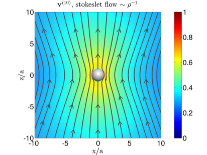
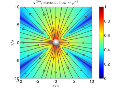
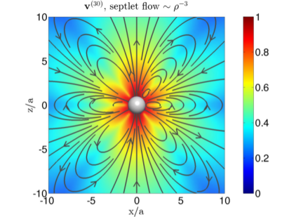
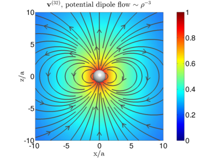
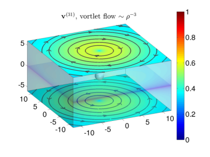
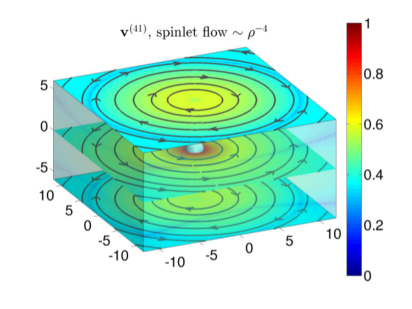
Figure 2: Axisymmetric and swirling flows due to traction and velocity modes on the surface of a sphere. Streamlines are overlaid on a pseudocolor plot of the logarithm of the magnitude of the fluid velocity in a planes containing the axis of the symmetry in the first four figures and in planes normal to it in the last two figures. The vectorial and septorial quadratic modes produce force-free, torque-free translation. The cubic spinlet mode produces force-free, torque-free rotation.

The system of linear equations that relate the velocity and traction coefficients are

$$4\pi\eta\,\mathbf{V}_{n}^{(l+1)} =-\sum_{m=1}^{N}\sum_{l^{\prime}=0}^{\infty}\left[\bm{G}_{nm}^{(l+1,\,l^{\prime}+1)}(\mathbf{R}_{n},\,\mathbf{R}_{m})\odot\mathbf{F}_{m}^{(l^{\prime}+1)}-\eta\bm{K}_{nm}^{(l+1,\,l^{\prime}+1)}(\mathbf{R}_{n},\,\mathbf{R}_{m})\odot\mathbf{V}_{m}^{(l^{\prime}+1)}\right],$$ (59)

where the matrix elements are given by double integrals of the Greens’ function and the stress tensor,

$$\bm{G}_{nm}^{(l+1,\,l^{\prime}+1)} =\frac{(2l+1)(2l^{\prime}+1)}{(4\pi a^{2})^{2}}\,\int{\mathbf{Y}}^{(l)}(\bm{\rho_{n}})\,\mathbf{G}(\mathbf{R}_{n}+\bm{\rho}_{n},\mathbf{R}_{m}+\bm{\rho_{m}})\,{\mathbf{Y}}^{(l^{\prime})}(\bm{\rho_{m}})\,\mathrm{d}S_{m}\mathrm{d}S,$$ (60a)

$$\bm{K}_{nm}^{(l+1,\,l^{\prime}+1)} =\frac{2l+1}{4\pi a^{2}(l^{\prime}-1)!(2l^{\prime}+1)!!}\,\int\mathbf{Y}^{(l)}(\bm{\rho_{n}})\mathbf{K}(\mathbf{R}_{n}+\bm{\rho}_{n},\mathbf{R}_{m}+\bm{\rho}_{m})\cdot\mathbf{n}\,\mathbf{Y}^{(l^{\prime})}(\bm{\rho_{m}})\,\mathrm{d}S_{m}\mathrm{d}S_{n}.$$ (60b)

As we show in Appendix D, these matrix elements can be expressed in terms of derivatives of the Greens’ functions and the stress tensor when the particle indices are not equal. For equal particle indices, the Green’s function matrix element is reduced to an angular integration and the stress tensor matrix element is the identity tensor. These results are collected below,

$$\bm{G}_{nm}^{(l+1,\,l^{\prime}+1)} =\left\{\begin{array}[]{l l l }\delta_{ll^{\prime}}\,\frac{(2l+1)}{(2\pi a)}\,\int d\Omega\,\mathbf{Y}^{(l)}(\widehat{\mathbf{\bm{\rho}}})\left(\mathbb{I}-\widehat{\mathbf{\bm{\rho}}}\widehat{\mathbf{\bm{\rho}}}\right)\mathbf{Y}^{(l)}(\widehat{\mathbf{\bm{\rho}}}),&m=n\\ \\ a^{l+l^{\prime}}\mathcal{F}_{m}^{l}\mathcal{F}_{m}^{l^{\prime}}\,\bm{\nabla}_{n}^{(l)}\,\bm{\nabla}_{m}^{(l^{\prime})}\,\mathbf{G}(\mathbf{R}_{n},\,\mathbf{R}_{m}),&m\neq n,\end{array}\right.$$ (61d)

$$\bm{K}_{nm}^{(l+1,\,l^{\prime}+1)} =\left\{\begin{array}[]{l l l }-\delta_{ll^{\prime}}\,4\pi\mathbb{I}\,\bm{\Delta}^{(l)},&m=n\\ \\ \frac{4\pi a^{(l+l^{\prime}+1)}}{(l^{\prime}-1)!(2l^{\prime}+1)!!}\mathcal{F}_{m}^{l}\mathcal{F}_{m}^{l^{\prime}}\,\bm{\nabla}_{n}^{(l)}\bm{\nabla}_{m}^{(l^{\prime}-1)}\,\mathbf{K}(\mathbf{R}_{n},\,\mathbf{R}_{m}),&m\neq n.\end{array}\right.$$ (61h)

We note that the diagonal ($m=n$) expression of the $\bm{K}^{(l+1,\,l^{\prime}+1)}_{nm}$ is defined for $l^{\prime}\geq 1$ and $\bm{K}^{(l+1,\,l^{\prime}+1)}_{nm}=0$ for $l^{\prime}=0$. We emphasize that the diagonal matrix elements are evaluated using the translational invariance of the Green’s function and the stress tensor. For the off-diagonal matrix elements, no such property is used, and the results, therefore, are valid for any bounding geometry.

The matrix elements having been determined, the rigid body motion can now be obtained from the formal solution of the previous section, in terms of the mobility and propulsion matrices, (10),

$$\mathbf{V}_{n} =\mathbf{V}_{n}^{a}+\sum_{m}^{N}\Big{[}\bm{\mu}^{\mathrm{TT}}_{nm}\cdot\mathbf{F}^{e}_{m}+\bm{\mu}^{\mathrm{TR}}_{nm}\cdot\mathbf{T}^{e}_{m}\Big{]}+\sum_{m\neq n}^{N}\sum_{l=1}^{\infty}\left[\bm{\pi}_{nm}^{(\mathrm{T},\,l+1)}\odot\mathbf{V}_{m}^{(l+1)}\right],$$ (62a)

$$\bm{\Omega}_{n} =\bm{\Omega}_{n}^{a}+\sum_{m}^{N}\Big{[}\bm{\mu}^{\mathrm{RT}}_{nm}\cdot\mathbf{F}^{e}_{m}+\bm{\mu}^{\mathrm{RR}}_{nm}\cdot\mathbf{T}^{e}_{m}\Big{]}+\sum_{m\neq n}^{N}\sum_{l=1}^{\infty}\left[\bm{\pi}_{nm}^{(\mathrm{R},\,l+1)}\odot\mathbf{V}_{m}^{(l+1)}\right].$$ (62b)

The active velocity $\mathbf{V}^{a}_{n}$ and active angular velocity $\bm{\Omega}_{n}^{a}$ are

$$4\pi a^{2}\,\mathbf{V}_{n}^{a} =-\int\mathbf{v}^{a}(\mathbf{r}_{n})\,\mathrm{d}S_{n},$$ (63a)

$$4\pi a^{2}\,\bm{\Omega}^{a}_{n} =-\frac{3}{2a}\int\widehat{\mathbf{\bm{\rho}}}_{n}\times\mathbf{v}^{a}(\mathbf{r}_{n})\,\mathrm{d}S_{n},$$ (63b)

the mobility matrices are

$$8\pi\eta\,\bm{\mu}_{nm}^{\mathrm{TT}} =\delta_{nm}\bm{G}^{(1,\,1)}_{nn}+\left(1-\delta_{nm}\right)\Big{(}\bm{G}^{(1,\,1)}_{nm}-\big{[}\mathsf{G}^{\mathrm{LH}}(\mathsf{G}^{\mathrm{HH}})^{-1}\mathsf{G}^{\mathrm{HL}}\big{]}_{nm}^{(1,\,1)}\Big{)},$$ (64a)

$$8\pi\eta\,\bm{\mu}_{nm}^{\mathrm{TR}} =\frac{1}{2}\bm{\epsilon}:\left(1-\delta_{nm}\right)\Big{(}\bm{G}^{(1,\,2)}_{nm}-\big{[}\mathsf{G}^{\mathrm{LH}}(\mathsf{G}^{\mathrm{HH}})^{-1}\mathsf{G}^{\mathrm{HL}}\big{]}_{nm}^{(1,\,2)}\Big{)},$$ (64b)

$$8\pi\eta\,\bm{\mu}_{nm}^{\mathrm{RT}} =\frac{1}{2}\bm{\epsilon}:\left(1-\delta_{nm}\right)\Big{(}\bm{G}^{(2,\,1)}_{nm}-\big{[}\mathsf{G}^{\mathrm{LH}}(\mathsf{G}^{\mathrm{HH}})^{-1}\mathsf{G}^{\mathrm{HL}}\big{]}_{nm}^{(2,\,1)}\Big{)},$$ (64c)

$$8\pi\eta\,\bm{\mu}_{nm}^{\mathrm{RR}} =\frac{1}{4}\delta_{nm}\bm{G}^{(2,\,2)}_{nn}+\frac{1}{4}\left(1-\delta_{nm}\right)\Big{(}\bm{G}^{(2,\,2)}_{nm}-\big{[}\mathsf{G}^{\mathrm{LH}}(\mathsf{G}^{\mathrm{HH}})^{-1}\mathsf{G}^{\mathrm{HL}}\big{]}_{nm}^{(2,\,2)}\Big{)},$$ (64d)

and the propulsion matrices are

$$8\pi\,\bm{\pi}_{nm}^{(\mathrm{T},\,l+1)} =\bm{K}^{(1,\,l+1)}_{nm}+\big{[}\mathsf{G}^{\mathrm{LH}}(\mathsf{G}^{\mathrm{HH}})^{-1}(4\pi\,\mathbb{I}-\mathsf{K}^{\mathrm{HH}})\big{]}^{(1,\,l+1)}_{nm},$$ (65a)

$$8\pi\,\bm{\pi}_{nm}^{(\mathrm{R},\,l+1)} =\bm{K}^{(2,\,l+1)}_{nm}+\big{[}\mathsf{G}^{\mathrm{LH}}(\mathsf{G}^{\mathrm{HH}})^{-1}(4\pi\,\mathbb{I}-\mathsf{K}^{\mathrm{HH}})\big{]}^{(2,\,l+1)}_{nm}.$$ (65b)

The above expressions are generalizations of Stokes law, which expresses the linearity of tractions and velocities, to the motion of $N$ active particles and are central results of this section.

It is useful to compare these results with existing results for computing many-body hydrodynamic interactions of spheres. In the absence of active velocities the boundary condition reduces to the usual no-slip boundary condition on the surface of each sphere. Then, there is no contribution from the second integral of the boundary integral representation and we obtain a single-layer formulation, first used by Zick and Homsy zick1982stokes , for computing the mobility of a periodic suspension. We should emphasise that Zick and Homsy used a reducible polynomial basis, in which redundant polynomials have to be manually removed from the sum. In contrast, the tensorial spherical harmonics are irreducible and, therefore, do not contain any redundant terms. In this limit of vanishing active velocity, truncating the Galerkin expansion to linear terms yields the method of computing far-field hydrodynamic interactions in the so-called “FTS” Stokesian dynamics method of Brady and colleagues durlofsky1987dynamic ; brady1988dynamic . This low-order truncation has been subsequently extended upto to $7$-th order in polynomials by Ichiki ichiki2002improvement . However, Ichiki’s extension requires six separate steps to relate the velocity coefficients to the traction coefficients. In contrast, the method provided here, since it uses identical basis functions for both velocity and traction, directly provides expressions for the coefficient matrices and the problem is reduced, directly, to solving the linear system. The extension of Stokesian dynamics method to active particles and its comparison to the method presented here, has been been done in section VI.

Returning to the case of active velocities, several authors have used the method of reflections for computing hydrodynamic interactions between pairs of spheres. Keh and Chen chen1988electrophoresis ; keh1995particle consider both the electrophoretic and thermophoretic interactions between particle pairs, computed to $\mathcal{O}(\rho^{-7})$ in particle separation $\rho$. Anderson anderson1981concentration has computed the change in the electrophoretic mobility in an infinite suspension as a function of volume fraction using the superposition approximation. Rider and O’Brien rider1993dynamic computed the AC electrophoretic mobility as a function of volume fraction and frequency of applied field, again in the superposition approximation. None of these papers have recognised, though, that hydrodynamic interactions between active particles can be completely described by propulsion matrices, nor have any of them provided a recipe for their evaluation, both of which have been accomplished in this paper.

IV Minimal truncation and superposition approximation

In this section, we consider a truncated version of the theory developed in the previous section, that retains the essential aspects of the hydrodynamic interactions between active spheres. Our truncation retains the least number of terms that are necessary to produce force-free translations and torque-free rotations of a single active spheres and to include all long-ranged contributions to the hydrodynamic interaction between many active spheres. It is, in this sense, a minimally truncated version of the general theory of the previous section. As we now show, expanding the boundary fields to cubic order in surface polynomials, that is retaining terms up to $\mathbf{Y}^{(3)}(\widehat{\mathbf{\bm{\rho}}})$, provides the desired minimal truncation.

In this minimal truncation, only terms corresponding to $l=0,1,2,3$ in (38) are retained

$$4\pi a^{2}\,\mathbf{f}(\mathbf{R}+\bm{\rho})=\Big{[}\mathbf{F}^{(1)}+3\,\mathbf{F}^{(2)}\odot\mathbf{Y}^{(1)}(\widehat{\mathbf{\bm{\rho}}})+5\,\mathbf{F}^{(3)}\odot\mathbf{Y}^{(2)}(\widehat{\mathbf{\bm{\rho}}})+7\,\mathbf{F}^{(4)}\odot\mathbf{Y}^{(3)}(\widehat{\mathbf{\bm{\rho}}})\Big{]},$$ (66a)

$$\mathbf{v}(\mathbf{R}+\bm{\rho})=\Big{[}\mathbf{V}^{(1)}+\mathbf{V}^{(2)}\odot\mathbf{Y}^{(1)}(\widehat{\mathbf{\bm{\rho}}})+\frac{1}{6}\,\mathbf{V}^{(3)}\odot\mathbf{Y}^{(2)}(\widehat{\mathbf{\bm{\rho}}})+\frac{1}{90}\,\mathbf{V}^{(4)}\odot\mathbf{Y}^{(3)}(\widehat{\mathbf{\bm{\rho}}})\Big{]}.$$ (66b)

The reducible traction coefficients are expressed in terms of their irreducible parts as (40a)

$$\mathbf{F}^{(1)} =-\mathbf{F}^{e},$$ (67a)

$$a\,\mathbf{F}^{(2)} =\mathbf{S}+\frac{1}{2}\bm{\epsilon}\cdot\mathbf{T}^{e},$$ (67b)

$$a^{2}\,\mathbf{F}^{(3)} =\mathbf{\Gamma}-\frac{2}{3}\bm{\Delta}^{(2)}\odot\left(\bm{\epsilon}\cdot\mathbf{\Psi}\right)+\frac{3}{5}\bm{\Delta}^{(2)}\odot\bm{\delta}\mathbf{D},$$ (67c)

$$a^{3}\,\mathbf{F}^{(4)} =\mathbf{\Theta}-\frac{3}{4}\bm{\Delta}^{(3)}\odot\left(\bm{\epsilon}\cdot\mathbf{\Lambda}\right)+\frac{6}{7}\bm{\Delta}^{(3)}\odot\bm{\delta}\mathbf{\Xi},$$ (67d)

while the reducible velocity coefficients are, similarly, expressed in terms of their irreducible parts as (40b)

$$\mathbf{V}^{(1)} =\mathbf{V}-\mathbf{V}^{a},$$ (68a)

$$\frac{1}{a}\,\mathbf{V}^{(2)} =\bm{s}-\bm{\epsilon}\cdot(\mathbf{\Omega}-\mathbf{\Omega}^{a}),$$ (68b)

$$\frac{1}{a^{2}}\,\mathbf{V}^{(3)} =\bm{\gamma}-\frac{2}{3}\bm{\Delta}^{(2)}\odot\left(\bm{\epsilon}\cdot\bm{\psi}\right)+\frac{3}{5}\bm{\Delta}^{(2)}\odot\bm{\delta}\bm{d},$$ (68c)

$$\frac{1}{a^{3}}\,\mathbf{V}^{(4)} =\bm{\theta}-\frac{3}{4}\bm{\Delta}^{(3)}\odot\left(\bm{\epsilon}\cdot\bm{\lambda}\right)+\frac{6}{7}\bm{\Delta}^{(3)}\odot\bm{\delta}\bm{\xi}.$$ (68d)

Here, $\mathbf{F}^{e}$, $\mathbf{T}^{e}$ and $\mathbf{S}$ are the familiar force, torque and stresslet strengths. $\mathbf{D}$, $\mathbf{\Psi}$ and $\mathbf{\Gamma}$ are the irreducible parts of the quadratic coefficients $\mathbf{F}^{(3)}$. They are irreducible tensors of rank 1, 2, and 3 as expected from angular momentum algebra. Similarly, $\mathbf{\Theta}$, $\mathbf{\Lambda}$ and $\mathbf{\Xi}$ are the irreducible parts of the cubic coefficients $\mathbf{F}^{(4)}$, and again, are tensors of rank 2, 3 and 4 coope1965 ; jerphagnon1970 ; jerphagnon1978 ; andrews1982 . The respective velocity coefficients are written in lower case. The flow expression (44) for a single particle for each $l,\,\sigma$ is given in table (2). The coefficients are linear combinations of the traction and velocity coefficients, to four of which we give explicit names

$$\mathbf{Q}^{(20)} =\mathbf{F}^{(20)}-\frac{8\pi\eta a}{3}\,\mathbf{V}^{(20)} \text{(Stresslet)},$$ (69a)

$$\mathbf{Q}^{(30)} =\mathbf{F}^{(30)}-\frac{8\pi\eta a}{15}\,\mathbf{V}^{(30)} \text{(Septlet)},$$ (69b)

$$\mathbf{Q}^{(31)} =\mathbf{F}^{(31)}-\frac{16\pi\eta a}{45}\,\mathbf{V}^{(31)} \text{(Vortlet)},$$ (69c)

$$\mathbf{Q}^{(41)} =\mathbf{F}^{(41)}-\frac{\pi\eta a}{35}\mathbf{V}^{(41)} \text{(Spinlet)}.$$ (69d)

Recalling the definition of the expansion coefficients, (39), we find that

$$a\mathbf{Q}^{(20)}= \int\left[\frac{1}{2}\left(\mathbf{f}\,{\bm{\rho}}+\left(\mathbf{f}\,{\bm{\rho}}\right)^{{T}}\right)-{\eta}\,\left(\mathbf{v}\,\widehat{\bm{\rho}}+\left(\mathbf{v}\,\widehat{\bm{\rho}}\right)^{{T}}\right)\right]\mathrm{d}S,$$ (70)

which, as we mentioned earlier, is the stresslet batchelor1970 introduced by Landau and Lifshitz landau1987fluid . The direct formulation of the boundary integral equation used here yields this combination in a natural manner and clearly shows the origin of each of the contributions from the Green’s function and the stress tensor integrals. It also provides a natural extension of this combination for expansion coefficients for any value of $l$ and $\sigma$. The three combinations explicitly named in the above, are particularly useful for the minimal description of spheres with active boundary layers. Their significance is as follows. The septlet is a third rank irreducible tensor and its flow decays as $1/\rho^{3}$. The vortlet and spinlet are, respectively, second rank and third rank irreducible tensors. They are, respectively, the leading and next to leading order terms that produce torque-free swirling flows. All these flows are plotted in figure 2 when the expansion tensors are uniaxial.

The irreducible traction and velocity coefficients are related by the solution of the diagonal part of (59), and on using (61d) and (61h), we find that the relation is both diagonal and scalar,

$$8\pi\eta\,\mathbf{V}_{n}^{(l\sigma)}=\delta_{ll^{\prime}}\delta_{\sigma\sigma^{\prime}}\,G_{nn}^{(l\sigma,\,l\sigma)}\mathbf{F}_{n}^{(l^{\prime}\sigma^{\prime})}.$$ (71)

Explicitly, for each irreducible part we have

$$\mathbf{V} =\mathbf{V}^{a}+\frac{\mathbf{F}^{e}}{6\pi\eta\,a},\qquad~{}\qquad\mathbf{\Omega}=\mathbf{\Omega}^{a}+\frac{\mathbf{T}^{e}}{8\pi\eta\,a^{3}}$$ (72a)

$$\mathbf{S} =-\frac{20\pi\eta\,a^{3}}{3}\mathbf{s},\qquad\,~{}~{}\qquad\bm{\Gamma}=-\frac{7\pi\eta\,a^{5}}{6}\mathbf{\gamma},$$ (72b)

$$\bm{\Psi} =\frac{4\pi\eta\,a^{5}}{3}\bm{\psi},\qquad~{}~{}~{}~{}~{}\qquad\mathbf{D}=-2\pi\eta\,a^{5}\mathbf{d},$$ (72c)

$$\bm{\Lambda} =-\frac{2\pi\eta\,a^{7}}{15}\bm{\lambda}.\qquad$$ (72d)

The first of these equations shows that translation and rotation are possible in the absence of external forces and torques. In their absence, the strengths of the potential dipole and the spinlet are related to the active translation and rotational velocities. This is evident from the expressions of these coefficients given in Appendix (C).

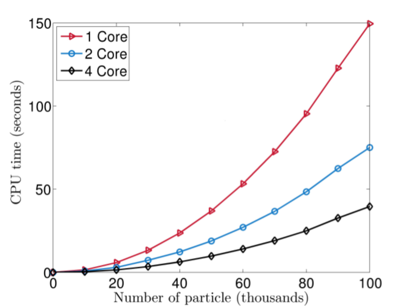
Figure 3: Benchmarks for calculation of stresslet propulsion matrix $\pi^{\mathrm{Ts}}$ in the superposition approximation on a 4-core machine using the PyStokes library pystokes . The present implementation of the library shows a linear scaling with the number of cores and quadratic scaling with the number of particles.

At each order $l$, there are $(2l+3)+(2l+1)+(2l-1)$ coefficients, from each of the three irreducible parts at that order. This gives $3$ coefficients at $l=0$, which are the three components of the force, $8$ coefficients at $l=1$, which are the $5$ components of the stresslet and $3$ components of the torque, $15$ coefficients at $l=2$, which are the $7$ components of the septet, $5$ components of the vortlet, and $3$ components of the potential dipole, and $21$ components at $l=3$. The linear system at this order of truncation, then, is of size $47N\times 47N$. For particles that number between tens to hundreds of thousands, this leads to a large numerical system that must be solved efficiently. The full details of the numerical implementation, using matrix-free iterative solvers and fast methods for matrix vector products, will be presented in a future contribution.

A significant simplification occurs at small concentrations, when the distance between particles is large compared to their radius. At small volume fractions, the mean distance between active particles is large compared to their size. The off-diagonal terms in the linear system, which depend on the distance between particles, are therefore small. Consequently, all off-diagonal terms in (61d, 61d) can be neglected, and the boundary integral equation becomes diagonal in the particle indices. The values of the tractions obtained from the one-body solution are, then, a good approximation for the many-body situation. At this order of approximation, the off-diagonal matrix elements in the mobility and propulsion matrices are negligible, and only the direct superposition contribution remains. This superposition approximation to the hydrodynamic interaction was first utilised by Kirkwood and Riseman kirkwood1948intrinsic in their study of polymer dynamics. With this approximation, the mobility matrices are

$$8\pi\eta\,\bm{\mu}_{nm}^{\mathrm{TT}} =\mathcal{F}_{n}^{0}\mathcal{F}_{m}^{0}\mathbf{G},~{}~{}~{}\qquad 8\pi\eta\,\bm{\mu}_{nm}^{\mathrm{TR}}=\frac{1}{2}\bm{\nabla}_{m}\times\mathbf{G},$$ (73a)

$$8\pi\eta\,\bm{\mu}_{nm}^{\mathrm{RT}} =\frac{1}{2}\bm{\nabla}_{n}\times\mathbf{G},\qquad 8\pi\eta\,\bm{\mu}_{nm}^{\mathrm{RR}}=\frac{1}{4}\bm{\nabla}_{n}\times\left(\bm{\nabla}_{m}\times\mathbf{G}\right),$$ (73b)

and the propulsion matrices are

$$8\pi\eta\,\bm{\pi}_{nm}^{\mathrm{Ts}} =C_{20}\,\mathcal{F}_{n}^{0}\mathcal{F}_{m}^{1}\bm{\nabla}_{m}\mathbf{G},\qquad~{}~{}~{}~{}~{}8\pi\eta\,\bm{\pi}_{nm}^{\mathrm{Rs}}=\frac{C_{20}}{2}\bm{\nabla}_{n}\times(\bm{\nabla}_{m}\mathbf{G}),$$ (74a)

$$8\pi\eta\,\bm{\pi}_{nm}^{\mathrm{T\gamma}} =C_{30}\,\mathcal{F}_{n}^{0}\mathcal{F}_{m}^{2}\bm{\nabla}_{m}\bm{\nabla}_{m}\mathbf{G},\qquad 8\pi\eta\,\bm{\pi}_{nm}^{\mathrm{R\gamma}}=\frac{C_{30}}{2}\bm{\nabla}_{n}\times(\bm{\nabla}_{m}\bm{\nabla}_{m}\mathbf{G}),\qquad$$ (74b)

$$8\pi\eta\,\bm{\pi}_{nm}^{\mathrm{T\psi}} =C_{31}\,\bm{\nabla}_{m}(\bm{\nabla}_{m}\times\mathbf{G}),\qquad~{}~{}8\pi\eta\,\bm{\pi}_{nm}^{\mathrm{R\psi}}=\frac{C_{31}}{2}\bm{\nabla}_{n}\times(\bm{\nabla}_{m}(\bm{\nabla}_{m}\times\mathbf{G})),$$ (74c)

$$8\pi\eta\,\bm{\pi}_{nm}^{\mathrm{Td}} =C_{32}\,\nabla_{m}^{2}\mathbf{G},\qquad\qquad\qquad~{}8\pi\eta\,\bm{\pi}_{nm}^{\mathrm{Rd}}=0$$ (74d)

$$8\pi\eta\,\bm{\pi}_{nm}^{\mathrm{T\lambda}} =C_{41}\,\bm{\nabla}_{m}\bm{\nabla}_{m}(\bm{\nabla}_{m}\times\mathbf{G}),~{}~{}~{}8\pi\eta\,\bm{\pi}_{nm}^{\mathrm{R\lambda}}=\frac{C_{41}}{2}\bm{\nabla}_{n}\times(\bm{\nabla}_{m}\bm{\nabla}_{m}(\bm{\nabla}_{m}\times\mathbf{G})).$$ (74e)

The coefficients $C_{l\sigma}$ are derived using (72). The specific values can be found in table 3. This level of approximation yields a very simple and direct method for studying active hydrodynamic interactions in dilute systems, through a pairwise summation of the mobility and propulsion matrices. We have implemented this superposition method, using a direct summation, in the PyStokes library pystokes . In figure 3, we have plotted the time for computing the contribution from a typical propulsion matrix, in this case the $l=1$ contribution. The library takes less than a minute for evaluating the velocity of $\mathcal{O}(10^{5})$ particles with prescribed stresslets. The method scales quadratically in the number of particles and linearly in the number of cores. Therefore, this provides method to compute the collective dynamics of a large number of hydrodynamically interacting active particles on multi-core computational architectures.

V Squirmers in a harmonic potential

Lighthill lighthill1952 and Blake blake1971a considered a sphere with a general axisymmetric slip velocity on the surface as a model for ciliated organisms. Retaining only tangential surface flows and the first two terms of their velocity expansion, the active velocity is

$$v^{a}_{\rho}=\widehat{\mathbf{\bm{\rho}}}\cdot\mathbf{v}^{a}=0,\qquad v^{a}_{\phi}=\widehat{\mathbf{\bm{\phi}}}\cdot\mathbf{v}^{a}=0,\qquad v^{a}_{\theta}=\widehat{\mathbf{\bm{\theta}}}\cdot\mathbf{v}^{a}=B_{1}\sin\theta+B_{2}\sin\theta\cos\theta.$$ (75a)

which can be written more compactly as,

$$\mathbf{v}^{a}=\left(\widehat{\mathbf{\bm{\rho}}}\widehat{\mathbf{\bm{\rho}}}-\mathbb{I}\right)\cdot\left[B_{1}\mathbf{p}+B_{2}\left(\mathbf{p}\mathbf{p}-\frac{\mathbb{I}}{3}\right)\cdot\widehat{\mathbf{\bm{\rho}}}\right],$$ (76)

where $\mathbf{p}$ is the orientation vector and $B_{1}$ and $B_{2}$ are constants. In terms of tensorial spherical harmonics, this is

$$\mathbf{v}^{a}=-\frac{2B_{1}}{3}\mathbf{p}-\frac{3B_{2}}{5}\left(\mathbf{p}\mathbf{p}-\frac{\mathbb{I}}{3}\right)\cdot\mathbf{Y}^{(1)}(\widehat{\mathbf{\bm{\rho}}})+\frac{B_{1}}{3}\mathbf{p}\mathbb{I}\odot\mathbf{Y}^{(2)}(\widehat{\mathbf{\bm{\rho}}})+\frac{B_{2}}{15}\left(\mathbf{p}\mathbf{p}-\frac{\mathbb{I}}{3}\right)\mathbb{I}\odot\mathbf{Y}^{(3)}(\widehat{\mathbf{\bm{\rho}}}).$$ (77)

Comparing (80) with the velocity expansion in tensorial spherical harmonics (38b), we note that $l=1,2,3$ contribute to the flow created by the squirmer. Also, the specific form of the coefficients of $\mathbf{Y}^{(l)}$ ensures that only $\mathbf{V}^{(20)}$, $\mathbf{V}^{(32)}$, $\mathbf{V}^{(42)}$ have non-vanishing contributions. These are

$$\mathbf{V}^{(10)} =\mathbf{V}-\mathbf{V}_{n}^{a},\qquad\mathbf{V}^{(20)}=-\frac{3}{5}B_{2}\left(\mathbf{p}\mathbf{p}-\frac{\mathbb{I}}{3}\right),$$ (78a)

$$\mathbf{V}^{(32)} =\frac{15}{2}\mathbf{V}^{a}_{n},\qquad\quad\mathbf{V}^{(42)}=\frac{140}{3}B_{2}\left(\mathbf{p}\mathbf{p}-\frac{\mathbb{I}}{3}\right),$$ (78b)

where the active translational velocity $\mathbf{V}^{a}_{n}$ of the squirmer is

$$\mathbf{V}^{a}_{n}=-\langle\mathbf{v}^{a}\rangle=\frac{2B_{1}}{3}\mathbf{p}.$$ (79)

This is an example of a non-trivial solution of the traction, which satisfies the zero-force, zero-torque constraint of (3), and yet, produces particle translation. The exterior flow due this boundary velocity consists of a stresslet, a potential dipole, and a degenerate octupole. Also, once the velocity coefficients are known then the tractions coefficients can be calculated using (61d) and (72).

$$4\pi a^{2}\,\mathbf{f}=4\pi\eta aB_{2}\left(\mathbf{p}\mathbf{p}-\frac{\mathbb{I}}{3}\right)\cdot\mathbf{Y}^{(1)}(\widehat{\mathbf{\bm{\rho}}})-12\pi\eta aB_{1}\mathbf{p}\cdot\mathbf{Y}^{(2)}(\widehat{\mathbf{\bm{\rho}}})-\frac{560}{3}\pi\eta aB_{2}\left(\mathbf{p}\mathbf{p}-\frac{\mathbb{I}}{3}\right)\odot\mathbf{Y}^{(3)}(\widehat{\mathbf{\bm{\rho}}}).$$ (80)

So the flow expression due to the squirmer is a linear combination of the flow due to these three terms as per table (2)

$$8\pi\eta\,\mathbf{v}=C_{20}\mathcal{F}_{m}^{1}\bm{\nabla}\mathbf{G}\odot\mathbf{Q}^{(20)}+C_{32}\nabla_{n}^{2}\mathbf{G}\odot\mathbf{Q}^{(32)}+C_{42}\bm{\nabla}\nabla^{2}\mathbf{G}\odot\mathbf{Q}^{(42)}.$$ (81)

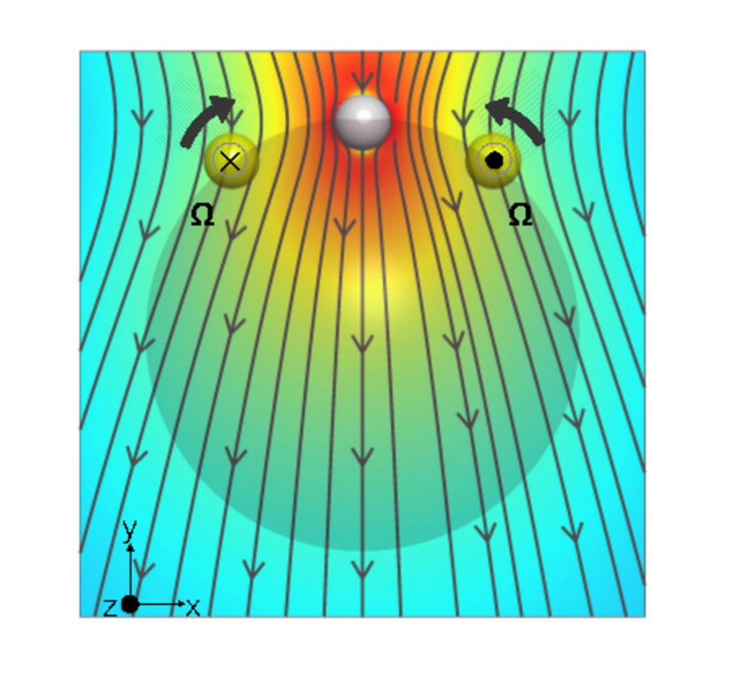
Figure 4: Flow generated by a test sphere (white) with a body force acting on it in the downward direction. This is the Stokeslet flow due to the particle at the north pole. The particles are situated on the surface of the schematic sphere. The two tracer particles (yellow ones) on the surface of the sphere then swim towards the test particle by orientating along it.

Active suspensions under confinement produces interesting dynamical phases nash2010 ; woodhouse2012 ; hennes2014self ; ezhilan2015transport . Here we study effects of confinement on hydrodynamically interacting finite sized squirmers of radius $a$. To do a minimal modeling of the squirmers, we truncate the velocity and angular velocity update equation (62) at $l=2$. The equations of the motion of the squirmers in the external harmonic potential is then

$$\dot{\mathbf{R}}_{n}= \underbrace{\mu^{\mathrm{TT}}_{nn}}_{\mathcal{O}(1)}(-\bm{\nabla}_{n}U)+\sum_{m\neq n}^{N}\bigg{[}\underbrace{\bm{\mu}^{\mathrm{TT}}_{nm}}_{\mathcal{O}(\rho^{-1})}\cdot(-\bm{\nabla}_{m}U)+\underbrace{\bm{\pi}_{nm}^{\mathrm{{Ts}}}}_{\mathcal{O}(\rho^{-2})}\odot\bm{s}_{m}+\underbrace{\bm{\pi}_{nm}^{\mathrm{{Td}}}}_{\mathcal{O}(\rho^{-3})}\odot\bm{d}_{m}\bigg{]}+\underbrace{\mathbf{V}^{a}_{n}}_{\mathcal{O}(1)},$$ (82a)

$${\mathbf{\Omega}}_{n}= \sum_{m\neq n}^{N}\bigg{[}\underbrace{\bm{\mu}^{\mathrm{RT}}_{nm}}_{\mathcal{O}(\rho^{-2})}\cdot(-\bm{\nabla}_{m}U)+\underbrace{\bm{\pi}_{nm}^{\mathrm{Rs}}}_{\mathcal{O}(\rho^{-3})}\odot\bm{s}_{m}\bigg{]},$$ (82b)

where $U$ is the potential due to the external force on each particle and the active velocity $\mathbf{V}^{a}_{n}=v_{s}\mathbf{p}_{n}$, where $v_{s}$ is the squirmer speed. We use the following uniaxial parametrization for the stresslet $\bm{s}$ and potential dipole $\bm{d}$,

$$\bm{s}=s_{0}\left(\mathbf{p}\mathbf{p}-\frac{1}{3}\mathbb{I}\right),\qquad\bm{d}=d_{0}\mathbf{p},$$ (83)

where $s_{0}$ and $d_{0}$ are stresslet and potential dipole strengths respectively. Since the particles are harmonically confined, the force due to the potential is the usual spring force $\mathbf{F}_{n}=-\bm{\nabla}_{n}U=-k\mathbf{R}_{n}$, where $k$ is the stiffness of the trap.

The equation describing the motion of a single passive particle in harmonic trap of spring constant $k$ can be written as,

$$\mathbf{\dot{R}}=\mu_{nn}^{\mathrm{TT}}\mathbf{F}^{e}=\frac{\mathbf{F^{e}}}{6\pi\eta a}=-\frac{k\mathbf{R}}{6\pi\eta a}.$$ (84)

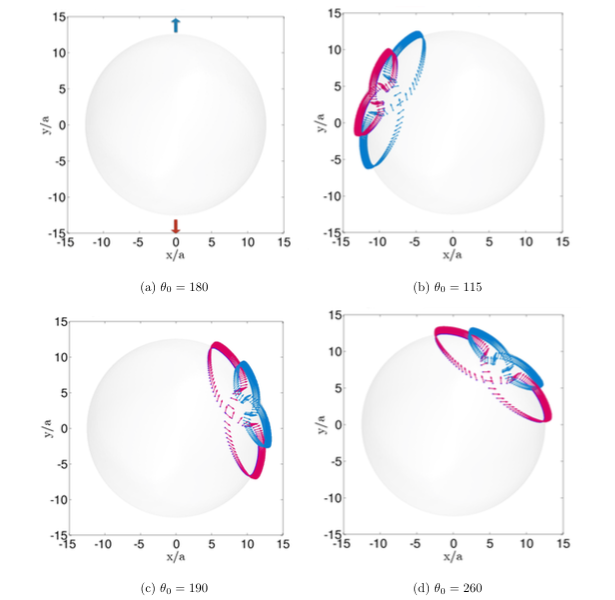
Figure 5: Dynamics of two particles in a harmonic trap. The particles are initialised on the surface of the sphere, with radius $R^{*}=\mathcal{A}a=12.56a$ (indicated by a schematic sphere), which is their stable state without HI. The first particle (blue) is initialised at the north pole and the second particle is kept at an angle $\theta_{0}$ measured in anticlockwise direction from the position of the first particle. In panel (a) $\theta_{0}=180$ and hence the angular velocity (85) of each particle is identically zero and hence there is no dynamics. In panel (b) $\theta_{0}=115$ and particles form a closed 8-like orbit. In panel (c) and (d), the final orbit is plotted for $\theta_{0}$ taking the values 190 and 260. It can be thus seen that two particle dynamics depends critically on the initial condition. The axis of the orbit, thus formed, is also dependent on the initial conditions.

The given dynamical equation for the particle is solved exactly by, $\mathbf{R}(t)=\mathbf{R}_{0}e^{-t/\tau}$. So, there is a time scale, $\tau_{1}$ in the system, given by ${\tau}_{1}=\frac{6\pi\eta a}{k}$. This is the time scale due to the overdamped motion of the particle in a harmonic potential. The final stable state is where all the particles are near the origin of the harmonic potential. If the particle is active, there is an additional term due to the active velocity of the particle $\mathbf{\dot{R}}=-\frac{k\mathbf{R}}{6\pi\eta a}+v_{s}\mathbf{p}$. The stable state of this system is found by setting the right hand side to zero, which defines a radius of confinement given by, $R^{*}=\frac{6\pi\eta v_{s}}{k}a=\mathcal{A}a$, such that at the confinement radius, the net radial velocity of the particle is zero. The stable configuration is now inverted and hence in the long time limit all the particle are found on the surface of the sphere of radius $R^{*}$ tailleur2008statistical ; tailleur2009sedimentation ; nash2010 . So a system of the non-interacting squirmer will have a stable state on the surface of the sphere of the radius $R^{*}$. We use this as the initial condition for our simulations and study the evolution of this stable initial state once the hydrodynamic interactions are turned on.

The lowest order terms in the velocity update equation (82) are the self terms $\mu^{\mathrm{TT}}_{nn}(-\bm{\nabla}_{n}U)$ and $\mathbf{V}^{a}_{n}$. The lowest order term from the HI (hydrodynamic interactions) is the Stokeslet $\bm{\mu}^{\mathrm{TT}}_{nm}$ and decays inversely $\rho^{-1}$, as the distance between the particles increases. In figure 4, the flow due to a Stokeslet on the north pole of the schematic sphere, is plotted. It is shown that the two other particles, which are moving in the field of the Stokeslet on north pole, move towards the source sphere by orienting towards it. This observation is crucial for the motion of particles in the harmonic potential, as Stokeslet is the most dominant term in the velocity and angular velocity equations once a large number of particles are considered.

Here we discuss simplest possible treatment of the HI in the trap. Since we are working in the superposition approximation, the HI is pairwise additive, hence the two particles dynamics should give us insight for problem of many squirmers in the harmonic potential. Consider the $\mathcal{O}(1)$ terms in the position update equation, we see that the stable position is the surface of the sphere, which we take as the initial condition. So unless we rotate the particle towards the trap center, nothing interesting will happen. The angular equations then determine the stability of this state. The leading terms in the angular velocity equation are $\bm{\mu}_{nm}^{\mathrm{RT}}$ and $\bm{\mu}_{nm}^{\mathrm{Rs}}$ as the potential dipole does not contribute to the angular velocity.

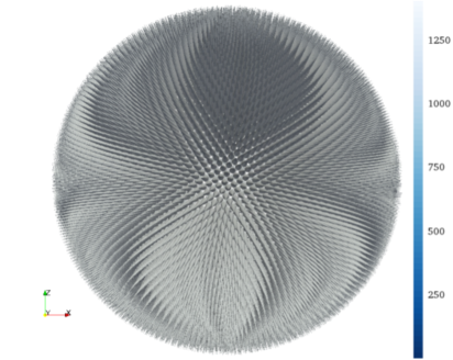
(a)  t=$0$

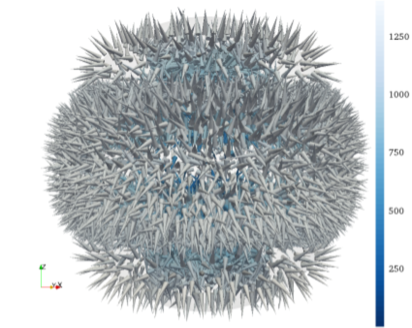
(b)  t=$\tau_{r}$

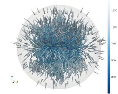
(c)  t=$2\tau_{r}$

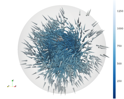
(d)  t=$8\tau_{r}$

Figure 6: Snapshots from the simulation of $10^{4}$ active particles, confined in a harmonic potential, at different times in terms of the rotational time scale $\tau_{r}=\frac{8\pi\eta a}{k}$. Squirmers are spherical particles with a radius $a$ and orientation vector $\mathbf{p}$. In the figures, the squirmers are denoted by cones located at the particle position and pointing in the direction of their orientation vector. The colormap shows the distance of the particles from the origin. The initial condition at time $t=0$ corresponding to a uniform distribution of the squirmers on the surface of trap sphere of radius $R^{*}=\mathcal{A}a=1256.6a$ (indicated by a schematic sphere). With time, steady-state convective currents are established and, the so-called self-assembled pump is formed in the system. See the supplementary material for the Movie. The simulations were performed using the PyStokes library pystokes .

For two particles the orientational dynamics is then given by

$$\mathbf{\dot{p_{1}}} =\left(\frac{-k\,(\mathbf{R_{2}}\times\mathbf{R_{1}})}{8\pi\eta\rho^{3}}+\frac{3C_{20}s_{0}\,(\mathbf{p}_{2}\cdot\bm{\rho})\,(\mathbf{p_{2}}\times\bm{\rho})}{\rho^{5}}\right)\times\mathbf{p}_{1},$$ (85a)

$$\dot{\mathbf{p_{2}}} =\left(\frac{-k\,(\mathbf{R_{1}}\times\mathbf{R_{2}})}{8\pi\eta\rho^{3}}+\frac{3C_{20}s_{0}\,(\mathbf{p}_{1}\cdot\bm{\rho})\,(\mathbf{p_{1}}\times\bm{\rho})}{\rho^{5}}\right)\times\mathbf{p}_{2}.$$ (85b)

Thus the angular velocity depends on the coordinates of other particles and not their orientations, at lowest order. This dominant term sets the rotational time scale in the system $\tau_{r}=\frac{8\pi\eta a}{k}$.

The dynamics of the two particles depends critically on their initial condition. If two particles are initialised on two diametrically opposite points then the there is no contribution to the angular velocity as $\bm{\mu}_{nm}^{\mathrm{RT}}$ and $\bm{\mu}_{nm}^{\mathrm{Rs}}$ are identically zero and hence the particle do not rotate. Therefore the dynamics is frozen. If the angle between particles is different from 180 degrees, then they form an 8-like structure which is a closed orbit. In figure 5 we have plotted the closed orbits formed by a system of two particles. The two-particle dynamics is then strongly determined by the initial condition. As the angular velocity (85) of each particle is identically zero for $\theta_{0}=180$, there is no rotation for this initial condition. For any other initial angle between the particles, a closed orbit is formed. The axis of this orbit is dependent on the initial condition of the particles as can be seen in figure 5.

In figure 6, snapshots from the simulation of $10^{4}$ finite-sized active particles confined in a harmonic potential have been given at different times in terms of the rotational time scale $\tau_{r}=\frac{8\pi\eta a}{k}$, determined by the Stokeslet contribution to the angular velocity in (82). The initial condition at $t=0$ corresponding to a uniform distribution of the squirmers on the surface of the sphere of radius $R^{*}=\mathcal{A}a=1256.6a$. This corresponds to the stable distribution of active squirmers without HI. We see the destabilization of this structure through the reorientation induced by the HI. The system eventually obtains a steady-state of convective currents, the so-called self-assembled pump nash2010 . Eq. (82) show that the key ingredients necessary for the pumping state are (a) one-body self-propulsion and (b) two-body rotation from the vorticity of the Stokeslet induced in the trap. The interesting things happen near the surface of the particles when the particle can not go any further, as the radial velocity is zero and need a angular velocity to rotate them back. On account of the hydrodynamic interactions from other particles, the particles on the surface are rotated back to the center of the trap. The dynamics is strongly determined by the Stokeslet flow as given in figure 4. The particles tends to come together and move towards the center of the trap but as they approach the center their orientations are rotated and then the one-body active velocity terms start dominating in making them move back to the surface of the confining sphere. Again, as they move towards the confining sphere, the Stokeslet strength picks up and pulls the particle back. This results in a pump-like motion of a macroscopic number of particles inside the trap. We also see that the two particles form a closed orbit about the surface of the trap and hence in the $N$ particle limit the behavior should be qualitatively similar, which is indeed the case. Now since the number of particles is large, they tend to bring the particles more closer to the origin till the Stokeslet contribution are weak and the particles again start moving back to the surface of the confining sphere. We note that only the leading order terms in (82) are important and account for the self-assembled pump. Thus the necessary and sufficient condition to obtain the pumping state are one-body self-propulsion and two-body rotation from the vorticity of the Stokeslet induced in the trap.

VI Discussion and summary

In the preceding sections, we have developed a systematic theory for studying hydrodynamic interactions in active colloidal particles. It is instructive to compare our approach with existing descriptions of active matter. These can be broadly classified into kinematic theories that prescribe active motion, without considering the balance of mass, momentum, angular momentum and energy, and dynamic theories which derive the active motion from the balance of these conserved quantities. The models of Toner and Tu toner1995long , Vicsek vicsek1995novel , and Chate gregoire2004onset belong the former category, while those of Finlayson and Scriven finlayson1969 , Simha and Ramaswamy simha2002a , and Saintillan and Shelley saintillan2008a belong to the latter category ramaswamy2010 ; marchetti2013 ; cates2012diffusive . The models, both kinematic and dynamic, can be also be classified by the length and time scales at which they resolve matter. Hydrodynamic theories operate at the coarsest length and time scales, and retain only variables that relax slowly. Kinetic theories operate at smaller length and time scales and contain in them the hydrodynamic description. Finally, particulate models offer a scale of resolution higher than both of hydrodynamic and kinetic theories and offer a complementary description free of the requirement of a continuum limit.

In the context of the above classification, our approach is a momentum-conserving particulate model for active matter. Active motion in our approach is not prescribed by fiat, but appears as a consequence of the balance of forces and torques, both at the particle boundaries and in the bulk ambient fluid. The contact forces and torques at the boundary are supplied by non-equilibrium processes that occur in the boundary layer which appear, in our approach, as an active velocity. We parametrize this velocity in full generality, and thus, all possible forms of active motion that arise from boundary layer phenomena are, in principle, included in our description. The specificity is contained in the velocity expansion coefficients, which depend on additional fields like electrical or chemical potentials in physico-chemical contexts, or on the motility of organelles, like cilia, in biological contexts. Thus, our approach provides a generic framework for active matter without sacrificing specific detail.

The Stokesian dynamics method has been extended to active particles, as reviewed in the work of Koch and Subramanian koch2011 . In particular, Ishikawa et al. ishikawa2006 ; ishikawa2008development have considered spheres with axisymmetric slip velocities, truncated to the first two non-trivial contributions, and computed the far-field contribution to the rigid body motion in the superposition approximation, while using a lubrication approximation to compute the near-field contribution. In contrast, our work includes both axisymmetric and swirling components of the active velocity and does not make any separation of far-field and near-field hydrodynamic interactions. Ishikawa et al. also use boundary element method, that is, a collocation discretization of the single layer boundary integral equation, to compute near-field hydrodynamic interactions.

Momentum conservation in our approach can be enforced without the need for explicit fluid degrees of freedom. This is possible at low Reynolds numbers, as the momentum balance equation for the fluid reduces to an elliptic partial differential equation whose solution can be represented as integrals over the domain boundaries. In contrast to models that retain explicit fluid degrees of freedom to enforce momentum conservation ramachandran2006lattice ; nash2010 ; nash2008 ; jayaraman2012 ; delmotte2015large ; llopis2006dynamic , our approach eliminates explicit fluid degrees of freedom and yet retains momentum conservation. Momentum conservation is enforced at the boundaries and is automatically ensured in the bulk through the integral representation. This reduction of the three-dimensional partial differential equation to a two-dimensional integral equation leads to efficient numerical methods for dynamic simulations of active particles.

Squirmers have been studied previously in the work of Pagonabarraga and Llopis llopis2006dynamic using lattice Boltzmann (LB) methods. They subtract a constant amount of momentum with fixed magnitude from the fluid, in a solid cone, which lie in predefined direction of motion of the particle. The subtracted momentum is then added to the active particle, such that momentum conservation is ensured. In another work Baskaran and Marchetti baskaran2009statistical model the active swimmer by a asymmetric rigid dumbbell composed of two Stokeslet differing in size, and hence the leading order hydrodynamic interaction in their case is $\mathcal{O}(\rho^{-2})$. They have then used a multipole expansion and a continuum analysis of the model. In contrast, we assume a spherical particle with active velocity specified on its surface which is then expanded in a Galerkin basis which leads to a systematic series of term which has a nice group-theoretic classification. And hence any generic mechanism generating the active velocity can be modeled in our scheme of expansion in a complete orthonormal Galerkin basis.

In this paper, we have provided explicit expression for the boundary integrals and matrix elements for a spherical active particles in an unbounded fluid. The extension to other geometries is accomplished by using a Green’s function appropriate to that geometry. Thus, active colloidal suspensions near plane walls and in periodic domains can be treated straightforwardly within this method. The periodic domain needs special care as a naive flow summation is conditionally convergent and a limiting procedure is needed to render the flow unconditionally convergent o1979method ; brady1988dynamic .

Hierarchical assemblies of active particles like single filaments with free jayaraman2012 or clamped laskar2013 boundary condition and active suspensions of short filaments pandey2014flow can be studied under this framework. Suspension rheology beyond the dilute can be studied systematically within our approach. Extensions of the present study in the above directions will be presented in future contributions.

We thank S. Ambikasaran, M. E. Cates, P. Chaikin, G. Date, A. Donev, L. Greengard, A. J. C. Ladd, I. Pagonabarraga, D. Pine, M. Shelley, H. A. Stone, and P. B. Sunil Kumar for many useful discussions; M. Rao, H. Stark, S. Saha, and R. Winkler for useful comments at the ICSM 2014 in Jaipur where this work was first presented; M. E. Cates and A. Donev for constructive remarks on an earlier version of this manuscript; and the Department of Atomic Energy, Government of India, for financial support.

Appendix A Boundary integral equation for electrostatics

The electrostatic problem of computing the potential due to $N$ spheres has a similar form as (6). Here, the potential is determined by Laplace’s equation,

$$\nabla^{2}\psi=0,$$ (86)

which has an integral representation jackson1962classical

$$4\pi\epsilon\,\psi(\mathbf{r}) =\sum_{m=1}^{N}\int\left[G(\mathbf{r},\mathbf{r_{m}})\,\sigma(\mathbf{r}_{m})-\epsilon\,n_{i}K_{i}(\mathbf{r},\mathbf{r}_{m})\,\psi(\mathbf{r}_{m})\,\right]\,\mathrm{d}S_{m},\quad\begin{subarray}{c}\displaystyle\mathbf{r}\in V\\ \\ \displaystyle\quad\,\mathbf{r}\in S_{m}\end{subarray}$$ (87)

$$G(\mathbf{r},\mathbf{r}^{\prime})=\frac{1}{\rho},\qquad K_{i}(\mathbf{r},\mathbf{r}^{\prime})=\nabla_{i}G=-\frac{\rho_{i}}{\rho^{3}}.$$ (88)

The potential in space, $\psi$, is expressed as integrals over the particle surfaces of the potential and its normal derivative $\mathbf{n}\cdot\bm{\nabla}\psi=\epsilon\sigma$, where $\epsilon$ is the permittivity and $\sigma$ is the surface charge density. Thus, there is a close analogy between the microhydrodynamic and electrostatic problems, with the correspondence

$$\mathbf{v}\leftrightarrow\psi,\qquad\mathbf{f}\leftrightarrow\sigma,\qquad\eta\leftrightarrow\epsilon.$$ (89)

The analogy is not wholly complete since $n_{i}K_{i}$ is the normal derivative of the Green’s function of the Laplace equation, while $n_{k}K_{ijk}$ is the sum of derivatives of the Green’s function of the Stokes equation and the pressure Green’s function. However, it does provide a heuristic for understanding microhydrodynamic phenomena guided by electrostatic analogies.

Appendix B Evaluation of boundary integrals

In this appendix, we outline the derivation of (44), from (43), which expresses the boundary integral in terms of the derivatives of the Green’s function. The key idea is to Taylor expand the Green’s function about the center of the sphere, and express the $l$-th degree polynomial of the radius vector in terms of tensorial spherical harmonics. Orthogonality of the harmonics and biharmonicity of the Green’s function reduces this infinite number of terms in the Taylor series to exactly two, giving the result in (44). To show these steps explicitly, the Taylor expansion is

$$\mathbf{G}(\mathbf{r},\,\mathbf{R}+\bm{\rho})= \sum_{l=0}^{\infty}\frac{1}{l!}(\bm{\rho}\cdot\bm{\nabla})^{(l)}\,\mathbf{G}(\mathbf{r},\,\mathbf{R}+\bm{\rho})\Big{|}_{\bm{\rho}=0},$$ (90)

where the expansion of the symmetric $l$-th degree polynomial in tensorial spherical harmonics is

$$(\bm{\rho}\cdot\bm{\nabla})^{(l)}= (\rho_{\alpha_{1}}\rho_{\alpha_{2}}\rho_{\alpha_{3}}\cdots\rho_{\alpha_{l}})(\nabla_{\alpha_{1}}\nabla_{\alpha_{2}}\nabla_{\alpha_{3}}\cdots\nabla_{\alpha_{l}}).$$ (91)

It should be noted that $(\rho_{\alpha_{1}}\rho_{\alpha_{2}}\rho_{\alpha_{3}}\cdots\rho_{\alpha_{l}})$ is not in its irreducible form. Now to make use of the orthogonality relation of (37) we convert the $\bm{\rho}^{(l)}$ to tensorial spherical harmonics using the following trick mazur1982

$$\rho_{i_{1}}\rho_{i_{2}}\rho_{i_{3}}\cdots\rho_{i_{l+2}}= a^{l}\frac{Y^{(l)}_{i_{1}i_{2}\cdots i_{l+2}}}{(2l-1)!!}+\frac{a^{l}}{2l-1}\sum_{\text{jk pairs}}\delta_{i_{j}i_{k}}\frac{Y^{(l-2)}_{i_{1}i_{2}\cdots i_{j-1}i_{j+1}\cdots i_{k-1}i_{k+1}\cdots i_{l}}}{(2l-5)!!}+\mathcal{O}(l-4).$$ (92)

from which it follows that

$$(\bm{\rho}\cdot\bm{\nabla})^{(l)}= a^{l}\left[\frac{\mathbf{Y}^{(l)}\bm{\nabla}^{(l)}}{(2l-1)!!}+\frac{1}{2l-1}\sum_{\text{jk pairs}}\frac{\mathbf{Y}^{(l-2)}\nabla^{2}\bm{\nabla}^{(l-2)}}{(2l-5)!!}+\mathcal{O}(l-4)\right].$$ (93)

Thus, only two terms remain on integration, giving

$$\bm{G}^{(l+1)}(\mathbf{r},\,\mathbf{R}) =a^{l}\bm{\Delta}^{(l)}\left(1+\frac{a^{2}}{4l+6}\nabla^{2}\right)\bm{\nabla}^{(l)}\,\mathbf{G}(\mathbf{r},\mathbf{R}).$$ (94)

Thus we see that the only terms surviving in the summation correspond to $l$ and the $l-2$ with a Laplacian and all the other terms go to zero by biharmonicity or due to odd powers of $\bm{\rho}$. Following the same method, it is straightforward to show that boundary integral contribution of the stress tensor to the flow is

$$\bm{K}^{(l+1)}(\mathbf{r},\,\mathbf{R}_{m})= \frac{4\pi a^{l+1}\bm{\Delta}^{(l)}}{(l-1)!(2l+1)!!}\left(1+\frac{a^{2}}{4l+6}\nabla_{m}^{2}\right){\bm{\nabla}_{m}}^{(l-1)}\mathbf{K}(\mathbf{r},\,\mathbf{R}_{m}),$$ (95)

Appendix C Irreducible parts of boundary integrals

The flow due to the boundary integral of the Green’s function is easily decomposed, using (40a), into its irreducible parts as

$$8\pi\eta\,\mathbf{v}^{\mathrm{G}}(\mathbf{r})= -a^{l}\sum_{l=0}^{\infty}\left(1+\frac{a^{2}}{4l+6}\nabla^{2}\right)\bm{\nabla}^{(l)}\mathbf{G}\odot\mathbf{F}^{(l)},$$

$$= -a^{l}\sum_{l=0}^{\infty}\Bigg{[}\left(1+\frac{a^{2}}{4l+6}\nabla^{2}\right)\bm{\Delta}^{(l+1)}\bm{\nabla}^{(l)}\mathbf{G}\odot\mathbf{F}^{(l0)}$$

$$-\frac{l}{l+1}\bm{\Delta}^{(l)}\left(\bm{\nabla}^{(l)}\times\mathbf{G}\right)\odot\mathbf{F}^{(l1)}$$

$$+\frac{l(l+1)}{2(2l+1)}\bm{\Delta}^{(l)}\bm{\nabla}^{(l-2)}\nabla^{2}\mathbf{G}\odot\mathbf{F}^{(l2)}\Bigg{]},$$ (96)

The boundary integral of the stress tensor can be reduced to the same form by using (40b). Writing the double layer contribution in the index notation.

$$8\pi\eta\,v^{\mathrm{K}}_{i}(\mathbf{r}) =\eta\sum_{l=0}^{\infty}\left[\left(1+\frac{a^{2}}{4l+6}\nabla^{2}\right)\nabla_{\alpha_{1}}\dots\nabla_{\alpha_{l-1}}K_{jik}V_{jk\alpha_{1}\dots\alpha_{l-1}}\right],$$ (97)

Now we use the (40b) in the previous expression to simplify it. Lets first calculate the $\sigma=0$ contribution due to the double layer. Let consider

$$\nabla_{\alpha_{1}}\dots\nabla_{\alpha_{l-1}}K_{jik}\Delta^{(l)}V_{jk\alpha_{1}\dots\alpha_{l-2}}^{(l0)} =2\Delta^{(l)}\nabla_{k}\nabla_{\alpha_{1}}\dots\nabla_{\alpha_{l-1}}G_{ij}V_{jk\alpha_{1}\dots\alpha_{l-2}}^{(l0)},$$ (98)

$$\nabla_{\alpha_{1}}\dots\nabla_{\alpha_{l-1}}K_{jik}\Delta^{(l-1)}\epsilon_{jk\gamma}V_{\gamma\alpha_{2}\dots\alpha_{l-1}}^{(l1)} =\frac{2l-2}{l}\Delta^{(l-1)}\epsilon_{jk\gamma}\nabla_{k}\nabla_{\alpha_{1}}\dots\nabla_{\alpha_{l-1}}G_{ij},V_{jk\alpha_{1}\dots\alpha_{l-2}}^{(l1)},$$ (99)

$$\nabla_{\alpha_{1}}\dots\nabla_{\alpha_{l-1}}K_{jik}\Delta^{(l-1)}\delta_{jk}V_{\alpha_{2}\dots\alpha_{l-2}}^{(l2)} =-3\Delta^{(l-1)}\nabla_{\alpha_{3}}\dots\nabla_{\alpha_{l-1}}\nabla^{2}G_{i\alpha_{2}}V_{\alpha_{2}\dots\alpha_{l-2}}^{(l2)}.$$ (100)

So all the three terms contribute from all the $three$ of its parts. This can then be generalized to any $l\sigma$ as

$$8\pi\eta\,\mathbf{v}^{\mathrm{K}}(\mathbf{r})= \frac{4\pi a^{(l+1)}}{(l-1)!(2l+1)!!}\sum_{l=0}^{\infty}\Bigg{[}\left(1+\frac{a^{2}}{4l+6}\nabla^{2}\right)\bm{\Delta}^{(l+1)}\bm{\nabla}^{(l)}\mathbf{G}\odot\mathbf{V}^{(l0)}$$

$$-\frac{l(2l-2)}{l(l+1)}\bm{\Delta}^{(l)}\left(\bm{\nabla}^{(l)}\times\mathbf{G}\right)\odot\mathbf{V}^{(l1)}$$

$$-\frac{3l(l+1)}{2(2l+1)}\bm{\Delta}^{(l)}\bm{\nabla}^{(l-2)}\nabla^{2}\mathbf{G}\odot\mathbf{V}^{(l2)}\Bigg{]},$$ (101)

The two expressions due to single layer and double layer can then be added to obtain the fluid flow (45) in terms of the $\mathbf{Q}^{(l\sigma)}$. The expressions of $\mathbf{Q}^{l\sigma}$ is given in (58). We also provide the integral expressions below

$$a\mathbf{Q}^{(20)}= \int\left[\frac{1}{2}\left(\mathbf{f}\,{\bm{\rho}}+\left(\mathbf{f}\,{\bm{\rho}}\right)^{{T}}\right)-\eta\,\left(\mathbf{v}\,\widehat{\bm{\rho}}+\left(\mathbf{v}\,\widehat{\bm{\rho}}\right)^{{T}}\right)\right]\mathrm{d}S,$$ (102a)

$$a^{2}\mathbf{Q}^{(30)}= \int\left[\frac{1}{6}\left(\overbrace{\,\mathbf{f}\,{\bm{\rho}}{\bm{\rho}}\,}-\frac{2}{5}(\mathbf{f}\cdot{\bm{\rho}})\overbrace{{\bm{\rho}}\,\mathbb{I}}-\frac{1}{5}\overbrace{\mathbf{f}\,\mathbb{I}}\right)-\frac{2\eta a}{3}\left(\overbrace{\,\mathbf{v}\,\widehat{\bm{\rho}}\widehat{\bm{\rho}}\,}-\frac{2}{5}(\mathbf{v}\cdot\widehat{\bm{\rho}})\overbrace{\widehat{\bm{\rho}}\,\mathbb{I}}-\frac{1}{5}\overbrace{\mathbf{v}\,\mathbb{I}}\right)\right]\mathrm{d}S,$$ (102b)

$$a^{2}\mathbf{Q}^{(31)}= \int\left[\frac{1}{6}\left((\mathbf{f}\times{\bm{\rho}})\,{\bm{\rho}}+\left\{(\mathbf{f}\times{\bm{\rho}})\,{\bm{\rho}}\right\}^{{T}}\right)-\frac{4\eta a}{9}\left((\mathbf{v}\times\widehat{\bm{\rho}})\,\widehat{\bm{\rho}}+\left\{(\mathbf{v}\times\widehat{\bm{\rho}})\,\widehat{\bm{\rho}}\right\}^{{T}}\right)\right]\mathrm{d}S,$$ (102c)

$$a^{2}\mathbf{Q}^{(32)}= \int\left[\frac{1}{6}\left((\mathbf{f}\cdot{\bm{\rho}})\,{\bm{\rho}}-\frac{1}{3}\mathbf{f}\right)-\eta a\left((\mathbf{v}\cdot\widehat{\bm{\rho}})\,\widehat{\bm{\rho}}-\frac{1}{3}\mathbf{v}\right)\right]\mathrm{d}S,$$ (102d)

$$a^{3}\mathbf{Q}^{(41)}= \int\left[\frac{1}{45}\left(\overbrace{\,\big{(}\mathbf{f}\times{\bm{\rho}}\big{)}\,{\bm{\rho}}\,{\bm{\rho}}\,}-\frac{3}{5}\overbrace{\big{(}\mathbf{f}\times{\bm{\rho}}\big{)}\,\mathbb{I}\,}\right)-\frac{\eta a^{2}}{20}\left(\overbrace{\,\big{(}\mathbf{v}\times\widehat{\bm{\rho}}\big{)}\,\widehat{\bm{\rho}}\,\widehat{\bm{\rho}}\,}-\frac{3}{5}\overbrace{\big{(}\mathbf{v}\times\widehat{\bm{\rho}}\big{)}\,\mathbb{I}\,}\right)\right]\mathrm{d}S.$$ (102e)

	Single layer	Double layer	Total contribution
$C_{20}$	$\frac{20}{3}\pi\eta a^{3}$	$\frac{8}{3}\pi\eta a^{3}$	$\frac{28}{3}\pi\eta a^{3}$
$C_{21}$	$-\frac{1}{2}$		$-\frac{1}{2}$
$C_{30}$	$\frac{7}{6}\pi\eta a^{5}\,$	$\frac{4}{15}\pi\eta a^{5}\,$	$\frac{43}{30}\pi\eta a^{5}$,
$C_{31}$	$\frac{8}{9}\pi\eta a^{5}\,$	$\frac{32}{3}\pi\eta a^{5}\,$	$\frac{13}{9}\pi\eta a^{5}$
$C_{32}$	$\frac{4}{5}\pi\eta a^{5}$	-$\frac{8}{5}\pi\eta a^{5}$	$-\frac{4}{5}\pi\eta a^{5}$
$C_{41}$	- $\frac{1}{10}\pi\eta a^{7}\,$	- $12\pi\eta a^{7}$	-$\frac{121}{10}\pi\eta a^{7}$

Table 3: The coefficients $C_{l\sigma}$.

Appendix D Evaluation of matrix elements

The expression of the diagonal ($m=n$) matrix elements can be obtained by expanding the pressure vector, Green’s function and the stress tensor in Fourier series, and then evaluating the integrals of the matrix elements. The respective Fourier transforms of the pressure vector, Green’s function and the stress tensor are

$$\mathbf{p}(\mathbf{k})=\frac{-i\,8\pi\widehat{\mathbf{k}}}{k},$$ (103a)

$$\mathbf{G}(\mathbf{k})=8\pi\bigg{[}\frac{\mathbb{I}-\widehat{\mathbf{k}}\widehat{\mathbf{k}}}{k^{2}}\bigg{]},$$ (103b)

$$\mathbf{K}(\mathbf{k}) =i\,8\pi\bigg{[}\frac{\overbrace{\widehat{\mathbf{k}}\mathbb{I}}-2\widehat{\mathbf{k}}\widehat{\mathbf{k}}\widehat{\mathbf{k}}}{k}\bigg{]},$$ (103c)

where $\overbrace{\dots}$ implies complete symmetrization and $i$ is the unit imaginary number. The single layer diagonal elements can be then written as

$$\bm{G}_{nn}^{(l+1,\,l^{\prime}+1)} =\frac{(2l+1)(2l^{\prime}+1)}{(4\pi a^{2})^{2}}\,\int\frac{\mathrm{d}\mathbf{k}\,e^{i(\bm{\rho}-\bm{\rho}^{\prime})\cdot\mathbf{k}}}{(2\pi)^{3}}{\mathbf{Y}}^{(l)}(\bm{\rho})\,8\pi\left(\frac{\mathbb{I}-\widehat{\mathbf{k}}\widehat{\mathbf{k}}}{k^{2}}\right){\mathbf{Y}}^{(l^{\prime})}(\bm{\rho^{\prime}})\,\mathrm{d}S_{n}\mathrm{d}S_{n}.$$ (104)

The integration can be performed using the orthogonality of the tensorial spherical harmonics (37) and by doing the plane wave expansion

$$e^{i\mathbf{k}\cdot\bm{\rho}} =\sum_{q=0}^{\infty}\frac{(i)^{q}(2q+1)}{q!\left(2q-1\right)!!}j_{q}(k\rho)\left(\mathbf{Y}^{(q)}(\widehat{\mathbf{k}})\odot\mathbf{Y}^{(q)}(\widehat{\mathbf{\bm{\rho}}}).\right)$$ (105)

We can then use the orthogonality relation of the spherical Bessel function

$$\int_{0}^{\infty}j_{l}(ka)j_{l^{\prime}}(ka)\,\mathrm{d}k =\delta_{ll^{\prime}}\frac{\pi}{2a\,(2l+1)},$$ (106)

to obtain diagonal-matrix elements of the single layer

$$\bm{G}_{nn}^{(l+1,\,l^{\prime}+1)} =\delta_{ll^{\prime}}\,\frac{(2l+1)}{(2\pi a)}\,\int\mathbf{Y}^{(l)}(\widehat{\mathbf{\bm{\rho}}})\left(\mathbb{I}-\widehat{\mathbf{\bm{\rho}}}\widehat{\mathbf{\bm{\rho}}}\right)\mathbf{Y}^{(l)}(\widehat{\mathbf{\bm{\rho}}})\,d\Omega.$$ (107)

The double layer diagonal matrix elements are

$$\bm{K}_{nn}^{(l+1,\,l^{\prime}+1)} =\frac{i8\pi\,(2l+1)}{(4\pi a^{2})\,l^{\prime}!(2l^{\prime}-1)!!}\,\int\frac{e^{i(\bm{\rho}-\bm{\rho}^{\prime})\cdot\mathbf{k}}}{(2\pi)^{3}}{\mathbf{Y}}^{(l)}(\bm{\rho})\,\bigg{[}\frac{\overbrace{\widehat{\mathbf{k}}\mathbb{I}}-2\widehat{\mathbf{k}}\widehat{\mathbf{k}}\widehat{\mathbf{k}}}{k}\bigg{]}\cdot\widehat{\mathbf{\bm{\rho}^{\prime}}}\,{\mathbf{Y}}^{(l^{\prime})}(\bm{\rho^{\prime}})\,\mathrm{d}\mathbf{k}\,\mathrm{d}S_{n}\mathrm{d}S_{n}.$$ (108)

We now expand the plane wave in spherical Bessel function (105). The diagonal matrix elements of the double layer is then

$$\bm{K}_{nn}^{(l+1,\,l^{\prime}+1)} =i^{q-p+1}\frac{(2l+1)\left(2q+1\right)(2p+1)}{4\pi^{3}a^{2}\,l!\,q!p!\left((2p-1)!!\right)^{2}(2q-1)!!}$$

$$\int\mathrm{d}S_{n}\mathbf{Y}^{(l)}({\bm{\rho}})\mathbf{Y}^{(q)}({\bm{\rho}})\int\mathrm{d}k\,k\,j_{q}(ka)j_{p}(ka)$$

$$\int\mathrm{d}\bm{\Omega}_{\mathbf{k}}\,\mathbf{Y}^{(q)}({\mathbf{k}}_{n})\big{[}\overbrace{\mathbf{\widehat{\mathbf{k}}}\mathbb{I}}-2\mathbf{\widehat{\mathbf{k}}}\mathbf{\widehat{\mathbf{k}}}\mathbf{\widehat{\mathbf{k}}}\big{]}\mathbf{Y}^{(p)}({\mathbf{k}}_{n})\cdot\int\widehat{\mathbf{\bm{\rho}^{\prime}}}\,\mathbf{Y}^{(l^{\prime})}(\widehat{\mathbf{\bm{\rho}^{\prime}}})\,\mathbf{Y}^{(p)}(\widehat{\mathbf{\bm{\rho}^{\prime}}})\mathrm{d}S_{n}.$$ (109)

At this point we can use the orthogonality of tensorial spherical harmonics and the following identity of the spherical Bessel function

$$\int_{0}^{\infty}\mathrm{d}k\,k\,j_{p}(ka)j_{q}(ka) =\delta_{p+1,q}\frac{\pi}{4a^{2}}.$$ (110)

Also, the integration over the $m$-th surface can be performed using (92) along with orthogonality relation of (37). The diagonal contribution to the double layer thus reduces to

$$\bm{K}_{nn}^{(l+1,\,l^{\prime}+1)} =-\frac{(2l+1)}{l!\,(2l^{\prime}-1)!!}\int\mathrm{d}\bm{\Omega}_{\mathbf{k}}\,\mathbf{Y}^{(l^{\prime})}({\mathbf{k}}_{n})\left[\widehat{\mathbf{k}}\cdot\left(\overbrace{\mathbf{\widehat{\mathbf{k}}}\mathbb{I}}-2\mathbf{\widehat{\mathbf{k}}}\mathbf{\widehat{\mathbf{k}}}\mathbf{\widehat{\mathbf{k}}}\right)\right]\mathbf{Y}^{(l)}({\mathbf{k}}_{n}).$$ (111)

Now, (92) and the orthogonality of the tensorial spherical harmonics (37) can be used to simplify (111). We also note that $\widehat{\mathbf{\bm{k}}}\cdot\left(\overbrace{\mathbf{\widehat{\mathbf{k}}}\mathbb{I}}-2\mathbf{\widehat{\mathbf{k}}}\mathbf{\widehat{\mathbf{k}}}\mathbf{\widehat{\mathbf{k}}}\right)=\mathbb{I}$. And hence the diagonal contribution of double layer is $-4\pi\mathbb{I}$ at any order

$$\bm{K}_{nn}^{(l+1,\,l^{\prime}+1)} =-\delta_{ll^{\prime}}\,4\pi\mathbb{I}\,\bm{\Delta}^{(l)}.$$ (112)

The unknown traction coefficients can then be written in terms of known velocity coefficients using (37 and 92).

$$8\pi\eta\,(\mathbf{V}-\mathbf{V}^{a}) =\left[\,\frac{1}{(2\pi a)}\,\int d\Omega\,\mathbf{Y}^{(0)}(\widehat{\mathbf{\bm{\rho}}})\left(\mathbb{I}-\widehat{\mathbf{\bm{\rho}}}\widehat{\mathbf{\bm{\rho}}}\right)\mathbf{Y}^{(0)}(\widehat{\mathbf{\bm{\rho}}})\right]\cdot\mathbf{F}^{e}=\frac{4}{3a}\mathbf{F}^{e}.$$ (113)

$$8\pi\eta\,(\mathbf{\Omega}-\mathbf{\Omega}^{a}) =\left[\,\frac{3}{(4\pi a^{3})}\,\int d\Omega\,\mathbf{Y}^{(1)}(\widehat{\mathbf{\bm{\rho}}})\mathbf{Y}^{(1)}(\widehat{\mathbf{\bm{\rho}}})\right]\cdot\mathbf{T}^{e}=\frac{1}{a^{3}}\mathbf{T}^{e},$$ (114)

$$8\pi\eta\,\bm{s} =\left[\,\frac{3}{(2\pi a^{3})}\,\int d\Omega\,\mathbf{Y}^{(1)}(\widehat{\mathbf{\bm{\rho}}})\left(\mathbb{I}-\widehat{\mathbf{\bm{\rho}}}\widehat{\mathbf{\bm{\rho}}}\right)\mathbf{Y}^{(1)}(\widehat{\mathbf{\bm{\rho}}})\right]\odot\mathbf{S}=-\frac{6}{5a^{3}}\mathbf{S}.$$ (115)

The expressions can be similarly calculated for higher $l$. The off-diagonal elements can be calculated exactly by following the steps given in the boundary integral calculations (Appendix B).

References

- (1) J. L. Anderson. Annu. Rev. Fluid Mech., 21(1):61–99, 1989.
- (2) W. F. Paxton, S. Sundararajan, T. E. Mallouk, and A. Sen. Angew. Chem., Int. Ed., 45(33):5420–5429, 2006.
- (3) J. R. Blake. J. Fluid Mech., 46(1):199–208, 1971.
- (4) H. Helmholtz. Annalen der Physik, 243(7):337–382, 1879.
- (5) M. Smoluchowski. Bull. Int. Acad. Sci. Cracovie, 182-199, 1903.
- (6) B. V. Derjaguin, G. P. Sidorenkov, E. A. Zubashchenkov, and E. V. Kiseleva. Kolloidn. Zh, 9:335–47, 1947.
- (7) J. L. Anderson. J. Colloid Interface Sci., 82(1):248–250, 1981.
- (8) S. B. Chen and H. J. Keh. AIChE Journal, 34(7):1075–1085, 1988.
- (9) P. F. Rider and R. W. O’Brien. J. Fluid Mech., 257:607–636, 1993.
- (10) M. J. Lighthill. Commun. Pure. Appl. Math., 5(2):109–118, 1952.
- (11) R. W. Nash, R. Adhikari, J. Tailleur, and M. E. Cates. Phys. Rev. Lett., 104:258101, Jun 2010.
- (12) M. Hennes, K. Wolff, and H. Stark. Phys. Rev. Lett., 111(23):238104, 2014.
- (13) L. D. Landau and E. M. Lifshitz. Fluid mechanics, 2nd. London: Elsevier, 1987.
- (14) G. K. Batchelor. An introduction to fluid dynamics. Cambridge university press, 2000.
- (15) F. K. G. Odqvist. Mathematische Zeitschrift, 32:329–375, 1930.
- (16) O. A. Ladyzhenskaia. The mathematical theory of viscous incompressible flow. Mathematics and its applications. Gordon and Breach, 1969.
- (17) C. Pozrikidis. Boundary Integral and Singularity Methods for Linearized Viscous Flow. Cambridge University Press, Cambridge, 1992.
- (18) S. Kim and S. J. Karrila. Microhydrodynamics: Principles and Selected Applications. Dover Civil and Mechanical Engineering Series. Dover Publications, 2005.
- (19) P. Mazur and W. Van Saarloos. Physica A: Stat. Mech. Appl., 115(1):21–57, 1982.
- (20) K. C. Nunan and J. B. Keller. J. Fluid Mech., 142:269–287, 1984.
- (21) B. U. Felderhof. Physica A: Stat. Mech. Appl., 89(2):373–384, 1977.
- (22) B. Cichocki, B. U. Felderhof, K. Hinsen, E. Wajnryb, and J. Blawzdziewicz. J. Chem. Phys., 100(5):3780–3790, 1994.
- (23) K. Ichiki. J. Fluid Mech., 452:231–262, 2002.
- (24) A. J. C. Ladd. J. Chem. Phys., 88:5051, 1988.
- (25) L. Durlofsky, J. F. Brady, and G. Bossis. J. Fluid Mech., 180:21–49, 1987.
- (26) J. F. Brady, R. J. Phillips, J. C. Lester, and G. Bossis. J. Fluid Mech., 195:257–280, 1988.
- (27) G. Youngren and A. Acrivos. J. Fluid Mech., 69(02):377–403, 1975.
- (28) A. A. Zick and G. M. Homsy. J. Fluid Mech., 115:13–26, 1982.
- (29) H. Power and G. Miranda. SIAM J. Appl. Math., 47(4):689–698, 1987.
- (30) G. P. Muldowney and J. J. L. Higdon. J. Fluid Mech., 298:167–192, 1995.
- (31) U. Weinert. Arch. Rational Mech. Anal., 74(2):165–196, 1980.
- (32) P. Brunn. Rheol. Acta, 15(2):104–119, 1976.
- (33) S. Ghose and R. Adhikari. Phys. Rev. Lett., 112(11):118102, 2014.
- (34) W. K. Tung. Group theory in physics. World Scientific Publishing, 1985.
- (35) S. Hess and W. Köhler. Formeln zur tensor-rechnung. Palm & Enke, 1980.
- (36) R. Schmitz. Physica A: Stat. Mech.Appl., 102(1):161–178, 1980.
- (37) G. K. Batchelor. J. Fluid Mech., 41(3):545–570, 1970.
- (38) H. J. Keh and S. H. Chen. Chem. Eng. Sci., 50(21):3395–3407, 1995.
- (39) J. A. R. Coope, R. F. Snider, and F. R. McCourt. J. Chem. Phys., 43:2269, 1965.
- (40) J. Jerphagnon. Phys. Rev. B, 2(4):1091–1098, 1970.
- (41) J. Jerphagnon, D. Chemla, and R. Bonneville. Adv. Phys., 27(4):609–650, 1978.
- (42) D. L. Andrews and W. A. Ghoul. Phys. Rev. A, 25(5):2647, 1982.
- (43) J. G. Kirkwood and J. Riseman. J. Chem. Phys., 16(6):565–573, 1948.
- (44) R. Singh, A. Laskar, and R. Adhikari. PyStokes: Hampi, Nov 2014.
- (45) F. G. Woodhouse and R. E. Goldstein. Phys. Rev. Lett., 109(16):168105, 2012.
- (46) B. Ezhilan and D. Saintillan. arXiv:1504.02792, 2015.
- (47) J. Tailleur and M. E. Cates. Phys. Rev. Lett., 100(21):218103, 2008.
- (48) J. Tailleur and M. E. Cates. Europhys. Lett., 86(6):60002, 2009.
- (49) J. Toner and Y. Tu. Phys. Rev. Lett., 75(23):4326, 1995.
- (50) T. Vicsek, A. Czirók, E. Ben-Jacob, I. Cohen, and O. Shochet. Phys. Rev. Lett., 75(6):1226, 1995.
- (51) G. Grégoire and H. Chaté. Phys. Rev. Lett., 92(2):025702, 2004.
- (52) B. A. Finlayson and L. E. Scriven. Proc. Roy. Soc. A, 310(1501):183–219, 1969.
- (53) R. A. Simha and S. Ramaswamy. Phys. Rev. Lett., 89:058101, Jul 2002.
- (54) D. Saintillan and M. J. Shelley. Phys. Rev. Lett., 100:178103, 2008.
- (55) S. Ramaswamy. Annu. Rev. Condens. Mat. Phys., 1(1):323–345, 2010.
- (56) M. C. Marchetti, J. F. Joanny, S. Ramaswamy, T. B. Liverpool, J. Prost, M. Rao, and R. A. Simha. Rev. Mod. Phys., 85:1143–1189, 2013.
- (57) M. E. Cates. Rep. Prog. Phys., 75(4):042601, 2012.
- (58) D. L. Koch and G. Subramanian. Annu. Rev. Fluid Mech., 43:637–659, 2011.
- (59) T. Ishikawa, M. P. Simmonds, and T. J. Pedley. J. Fluid Mech., 568(1):119–160, 2006.
- (60) T. Ishikawa, J. T. Locsei, and T. J. Pedley. J. Fluid Mech., 615:401–431, 2008.
- (61) I. Llopis and I. Pagonabarraga. Europhys. Lett., 75(6):999, 2006.
- (62) S. Ramachandran, P. B. Sunil Kumar, and I. Pagonabarraga. Eur. Phys. J. E, 20(2):151–158, 2006.
- (63) R. W. Nash, R. Adhikari, and M. E. Cates. Phys. Rev. E, 77:026709, Feb 2008.
- (64) B. Delmotte, E. Keaveny, F. Plouraboue, and E. Climent. arXiv:1501.02912, 2015.
- (65) G. Jayaraman, S. Ramachandran, S. Ghose, A. Laskar, M. Saad Bhamla, P. B. Sunil Kumar, and R. Adhikari. Phys. Rev. Lett., 109(15):158302, 2012.
- (66) A. Baskaran and M. C. Marchetti. PNAS, 106(37):15567–15572, 2009.
- (67) R. W. O’brien. J. Fluid Mech., 91(01):17–39, 1979.
- (68) A. Laskar, R. Singh, S. Ghose, G. Jayaraman, P. B. Sunil Kumar, and R. Adhikari. Sci. Rep., 3:1964, 2013.
- (69) A. Pandey, P. B. Sunil Kumar, and R. Adhikari. arXiv:1411.0278, 2014.
- (70) J. D. Jackson. Classical electrodynamics. Wiley, 1962.