The roles of a quantum channel on a quantum state

Abstract

When a quantum state undergoes a quantum channel, the state will be inevitably influenced. In general, the fidelity of the state is reduced, so is the entanglement if the subsystems go through the channel. However, the influence on the coherence of the state is quite different. Here we present some state-independent quantities to describe to what degree the fidelity, the entanglement and the coherence of the state are influenced. As applications, we consider some quantum channels on a qubit and find that the infidelity ability monotonically depends on the decay rate, but in usual the decoherence ability is not the case and strongly depends on the channel.

I Introduction

Quantum coherence or quantum superposition is one of the most fundamental feature of quantum mechanics that distinguishes the quantum world from the classical world. It is one of the main manifestation of quantumness in a single quantum system. For a composite quantum system, due to its tensor structure, quantum superposition could directly lead to quantum entanglement, another intriguing feature of quantum mechanics and the very important physical resource in quantum information processing [1]. In fact, safely speaking, quantum coherence is one necessary condition for almost all the mysterious features of a quantum state. For example, both entanglement and quantum discord that has attracted much attention recently [1-10], have been shown to be quantitatively related to some special quantum coherence [11,12]. However, when a quantum system undergoes a noisy quantum channel or equivalently interacts with its environment, the important quantum feature, i.e., the quantum decoherence, could decrease. It is obvious that whether decoherence happens strongly depends on the quantum channel and the state itself, but definitely a quantum channel describes the fate of quantum information that is transmitted with some loss of fidelity from the sender to a receiver. In addition, if the subsystem of an entangled state passes through such a channel, disentangling could happen and go even more quickly.

Decoherence as well as disentangling for composite systems has never been lack of concern from the beginning. A lot of efforts have been paid to decoherence in a wide range such as the attempts of understanding of decoherence [13,14], the dynamical behaviors of decoherence subject to different models [15-20], the reduction or even prevention of decoherence [21-23], the disentangling through various channels and so on [24-26]. Actually, most of the jobs can be directly or indirectly summarized as the research on to what degree a noisy quantum channel or the environment influences (mostly destroys) the coherence, the fidelity or entanglement of the given quantum system of interests. So it is important and interesting to consider how to effectively evaluate the ability of a quantum channel that leads to decoherence, the loss of fidelity of a quantum state, or disentangling of a composite system, in particular, independent of the state.

In this paper, we address the above issues by introducing three particular measure, the decoherence power, the infidelity power and the disentangling factor to describe the abilities, respectively. This is done by considering how much fidelity, coherence or entanglement (for composite systems) is decreased by the considered quantum channel on the average, acting on a given distribution of quantum state or the subsystem of an entangled state. This treatment has not been strange since the entangling power of a unitary operator as well as the similar applications in other cases was introduced [27,28]. However, because the calculation of the abilities of a quantum channel strongly depends on the structure of the quantum states which undergo the channel, the direct result is that only 2- dimensional quantum channel can be effectively considered. For the high dimensional quantum channels, one might have to consider these behaviors on a concrete state, which is analogous to that the entangling power can be only considered for the systems of two qubits [27]. These cases will not be covered in this paper. This paper is organized as follows. In Sec. II, we treat the quantum channel as the reduction mechanism of the fidelity and present the infidelity power accompanied by some concrete examples. In Sec. III, we consider how to influence the coherence of a state and give the decoherence power. Some examples are also provided. In Sec. IV, we analyze the potential confusion if we consider the decoherence of a mixed state and briefly discuss how to consider the influence of quantum channel on the subsystem of a composite quantum system. The conclusion is drawn in Sec. V.

II Infidelity power

II.1 Fidelity

When a quantum state undergoes a quantum channel, the state will generally be influenced. Although some particular features of the state could not be changed, the concrete form of the state, i.e., the fidelity, is usually changed. In order to give a description of the ability to which degree a quantum channel influences a quantum state, we would like to first consider the infidelity power of a quantum channel.

With fidelity of two states $\rho$ and $\rho^{\prime}$ mentioned, one could immediately come up with the fidelity defined by $F^{\prime}\left(\rho,\rho^{\prime}\right)=Tr\sqrt{\sqrt{\rho}\rho^{\prime}\sqrt{\rho}}$ or the trace distance defined by $D^{\prime}\left(\rho,\rho^{\prime}\right)=\left\|\rho-\rho^{\prime}\right\|_{1}$ with $\left\|A\right\|_{1}=Tr\sqrt{AA^{\dagger}}$ [29]. However, consider some given distribution of state $\rho$, one can find that the mentioned definitions are not convenient to derive a state-independent quantity. So we would like to consider another definition of the fidelity based on Frobenius norm $\left\|\cdot\right\|_{2}$.

Definition 1.-The fidelity of the state $\rho$ and $\rho^{\prime}$ is defined by

$$F\left(\rho,\rho^{\prime}\right)=1-\frac{1}{2}\left\|\rho-\rho^{\prime}\right\|_{2}^{2}.$$ (1)

It is clear that if and only if $\rho$ and $\rho^{\prime}$ are the same, the fidelity $F=1$. To proceed, we have to introduce a lemma.

Lemma 1. For any $n$-dimensional matrix $A$, and an $\left(n\otimes n\right)$-dimensional maximally entangled state in the computational basis $\left|\Phi_{n}\right\rangle=\sum\limits_{k}\frac{1}{\sqrt{n}}\left|kk\right\rangle$, the following relations hold:

$$\left(A\otimes\mathbf{1}_{n}\right)\left|\Phi_{n}\right\rangle=\left(\mathbf{1}_{n}\otimes A^{T}\right)\left|\Phi_{n}\right\rangle,$$ (2)

and

$$TrA=n\left\langle\Phi_{n}\right|\left(A\otimes\mathbf{1}_{n}\right)\left|\Phi_{n}\right\rangle.$$ (3)

Proof. The proof is direct, which is also implied in Ref. [27]. $\blacksquare$

Now, let $\$$ denote a quantum channel and $\rho^{\prime}=\$\left(\rho\right)$ denote the final state of $\rho$ going through the channel, the fidelity given in Eq. (1) can be rewritten as

$$F\left(\rho,\$\left(\rho\right)\right) = 1-\frac{1}{2}\left\|\rho-\$\left(\rho\right)\right\|_{2}^{2}$$ (4)

$$= 1-\frac{1}{2}Tr\rho^{2}-\frac{1}{2}Tr\$\left(\rho\right)^{2}+Tr\rho\$\left(\rho\right).$$

Based on Lemma 1, we can find that

$$Tr\rho\$\left(\rho\right)=n\left\langle\Phi_{n}\right|\rho\$\left(\rho\right)\otimes\mathbf{1}_{n}\left|\Phi_{n}\right\rangle$$

$$=n\left\langle\Phi_{n}\right|\rho\otimes\left[\$(\rho)\right]^{T}\left|\Phi_{n}\right\rangle$$

$$=nTr\left[\rho\otimes\rho^{\ast}\right]\left(\$\otimes\mathbf{1}_{n}\right)\left|\Phi_{n}\right\rangle\left\langle\Phi_{n}\right|$$

$$=n^{3}\left\langle\Phi_{n^{2}}\right|\left[\rho\otimes\rho^{\ast}\right]\left(\$\otimes\mathbf{1}_{n}\right)\left|\Phi_{n}\right\rangle\left\langle\Phi_{n}\right|\otimes\mathbf{1}_{n^{2}}\left|\Phi_{n^{2}}\right\rangle$$

$$=n^{3}Tr\left(\$\otimes\mathbf{1}_{n}\right)\left|\Phi_{n}\right\rangle\left\langle\Phi_{n}\right|\otimes\rho^{\ast}\otimes\rho$$

$$\times S_{23}\left(\left|\Phi_{n}\right\rangle\left\langle\Phi_{n}\right|\otimes\left|\Phi_{n}\right\rangle\left\langle\Phi_{n}\right|\right)S_{23}$$ (5)

and

$$Tr\$\left(\rho\right)^{2}=n\left\langle\Phi_{n}\right|\left[\$(\rho)\right]^{2}\otimes\mathbf{1}_{n}\left|\Phi_{n}\right\rangle$$

$$=nTr\left[\$(\rho)\otimes\rho^{\ast}\right]\left(\$\otimes\mathbf{1}_{n}\right)\left|\Phi_{n}\right\rangle\left\langle\Phi_{n}\right|$$

$$=n^{3}\left\langle\Phi_{n^{2}}\right|\left[\$(\rho)\otimes\rho^{\ast}\right]\left(\$\otimes\mathbf{1}_{n}\right)\left|\Phi_{n}\right\rangle\left\langle\Phi_{n}\right|\otimes\mathbf{1}_{n^{2}}\left|\Phi_{n^{2}}\right\rangle$$

$$=n^{3}\left\langle\Phi_{n^{2}}\right|\left(\$\otimes\mathbf{1}_{n}\right)\left|\Phi_{n}\right\rangle\left\langle\Phi_{n}\right|\otimes\left[\$(\rho)\right]^{T}\otimes\rho\left|\Phi_{n^{2}}\right\rangle$$

$$=n^{3}Tr\left\{\left(\$\otimes\mathbf{1}_{n}\right)\left|\Phi_{n}\right\rangle\left\langle\Phi_{n}\right|\otimes\rho^{\ast}\otimes\rho\right\}$$

$$\times S_{23}\left(\$\otimes\mathbf{1}_{n}\right)\left|\Phi_{n}\right\rangle\left\langle\Phi_{n}\right|\otimes\left|\Phi_{n}\right\rangle\left\langle\Phi_{n}\right|S_{23},$$ (6)

where we consider $\left|\Phi_{n^{2}}\right\rangle=S_{23}\left|\Phi_{n}\right\rangle\left|\Phi_{n}\right\rangle$ with $S_{23}$ representing the swapping operations between the 2nd and 3rd subsystems. Let

$$\left\{\begin{array}[]{c}W_{1}=S_{23}\left[\tilde{\$}\left(\varrho_{\Phi}\right)\otimes\varrho_{\Phi}\right]S_{23}\\ W_{2}=S_{23}\left[\varrho_{\Phi}\otimes\varrho_{\Phi}\right]S_{23}\\ Q_{1}=\tilde{\$}\left(\varrho_{\Phi}\right)\otimes\mathbf{1}_{n^{2}}\\ Q_{2}=\varrho_{\Phi}\otimes\mathbf{1}_{n^{2}}\end{array}\right.$$ (7)

with $\tilde{\$}\left(\varrho_{\Phi}\right)=\left(\$\otimes\mathbf{1}_{n}\right)\left|\Phi_{n}\right\rangle\left\langle\Phi_{n}\right|$ and $\varrho_{\Phi}=\left|\Phi_{n}\right\rangle\left\langle\Phi_{n}\right|$, and substitute Eq. (5) and Eq. (6) into Eq. (4), $F\left(\rho,\$\left(\rho\right)\right)$ can be rewritten as

$$F\left(\rho,\$\left(\rho\right)\right)=1-\frac{n^{3}}{2}Tr\left(\mathbf{1}_{n^{2}}\otimes\rho^{\ast}\otimes\rho\right)\mathcal{M}.$$ (8)

with

$$\mathcal{M}=\left[Q_{1}(W_{1}-W_{2})+\left(Q_{2}-Q_{1}\right)W_{2}\right].$$ (9)

Thus $\mathcal{M}$ only depends on the influence of the maximally entangled state $\left|\Phi_{n}\right\rangle$ through the considered quantum channel instead of the information of the state of interests. The infidelity power can be directly defined as the difference of fidelity before and after going through the channel subject to some given distribution. However, different distributions would lead to quite different infidelity power. In this paper, we restrict ourselves to the uniform distribution.

II.2 Infidelity power

In order to describe the difference between the fidelities of the state $\rho$ with and without quantum channel $\$$, we can use

$$\tilde{e}_{F}\left(\rho,\$\left(\rho\right)\right) = F\left(\rho,\rho\right)-F\left(\rho,\$\left(\rho\right)\right)$$ (10)

$$= \frac{n^{3}}{2}Tr\left(\mathbf{1}_{n^{2}}\otimes\rho^{\ast}\otimes\rho\right)\mathcal{M}.$$

Consider the uniform distribution $\mathcal{F}$ of the state $\rho$ [27], we can define the infidelity power as follows.

Definition 2. The infidelity power of the $n$-dimensional quantum channel $\$$ can be defined as

$$e_{\mathcal{F}}\left(\$\right)=\frac{n^{3}}{2}Tr\left(\mathbf{1}_{n^{2}}\otimes\mathcal{F}(\rho)\right)\mathcal{M},$$ (11)

with $\mathcal{F}(\rho)=\frac{1}{\Omega_{\mathcal{F}}}\int_{\mathcal{F}}\rho^{\ast}\otimes\rho du(\rho)$ where $\Omega_{\mathcal{F}}$ is some normalization factor, $du(\rho)$ denotes the measure over the state $\rho$ induced by the uniform distribution $\mathcal{F}$.

It is obvious that $\mathcal{F}(\rho)$ does not depend on the concrete form of a density matrix but only the dimension of the density matrices and the structure of the states. However, it is unfortunate that the structure of the high dimensional states is very complicated. It is difficult to describe a given distribution of such a state space. Therefore, we only present the concrete expression of $\mathcal{F}(\rho)$ for a system of qubit.

Theorem 1. The infidelity power of the quantum channel $\$$ on a qubit can be given by

$$\tilde{e}_{\mathcal{F}}\left(\$\right)=4Tr\left(\mathbf{1}_{n^{2}}\otimes\mathcal{F}(\rho)\right)\mathcal{M},$$ (12)

with

$$\mathcal{F}(\rho)=\frac{1}{5}\mathbf{1}_{4}\otimes\left(\mathbf{1}_{4}+\left|\Phi_{2}\right\rangle\left\langle\Phi_{2}\right|\right).$$ (13)

Proof. The density matrix of any qubit $\rho$ can be given in the Bloch representation as

$$\rho=\frac{1}{2}\left(\mathbf{1}_{2}+r\mathbf{n}\cdot\mathbf{\sigma}\right)$$ (14)

where $\mathbf{\sigma}=[\sigma_{x},\sigma_{y},\sigma_{z}]$ is the Pauli matrices, $\mathbf{n}=[\sin\theta\cos\varphi,\sin\theta\sin\varphi,\cos\theta]$ with $\theta$ the inclination and $\varphi$ the azimuth in the Bloch sphere, respectively, and $r$ is the radius. Since we suppose the state is distributed uniformly, the state density can be given by $r^{2}\sin\theta$. So one can easily find that

$$\Omega_{\mathcal{F}}=\int\limits_{0}^{1}r^{2}dr\int_{0}^{\pi}\sin\theta d\theta\int_{0}^{2\pi}d\varphi=\frac{4\pi}{3},$$ (15)

and

$$\mathcal{F}(\rho) = \frac{3}{16\pi}\int\limits_{0}^{1}r^{2}dr\int_{0}^{\pi}\sin\theta\int_{0}^{2\pi}\left[\mathbf{1}_{4}\right.+r\mathbf{n}\cdot\left(\mathbf{1}_{2}\otimes\mathbf{\sigma}+\mathbf{\sigma}\otimes\mathbf{1}_{2}\right)$$ (16)

$$+r^{2}\left.\left(\mathbf{n}\otimes\mathbf{n}\right)\cdot\left(\mathbf{\sigma}^{\ast}\otimes\mathbf{\sigma}\right)\right]d\varphi d\theta$$

$$= \frac{1}{4}\left[\mathbf{1}_{4}+\frac{1}{5}\left(\sigma_{x}\otimes\sigma_{x}-\sigma_{y}\otimes\sigma_{y}+\sigma_{z}\otimes\sigma_{z}\right)\right],$$

which is consistent with Eq. (13). The proof is completed. $\blacksquare$

II.3 Examples

As applications, we would like to calculate the infidelity power for a qubit of the depolarizing channel $\$_{d}$ given in Kraus representation as

$$M_{0}^{d}=\sqrt{1-p}\mathbf{1}_{2},M_{k}^{d}=\sqrt{\frac{p}{3}}\sigma_{k},k=1,2,3,$$ (17)

the phase-damping channel $\$_{p}$ given by

$$M_{0}^{p} = \sqrt{1-p}\mathbf{1}_{2},$$ (18)

$$M_{1}^{p} = \sqrt{p}\left(\begin{array}[]{cc}1&0\\ 0&0\end{array}\right),$$ (21)

$$M_{2}^{p} = \sqrt{p}\left(\begin{array}[]{cc}0&0\\ 0&1\end{array}\right),$$ (24)

the amplitude-damping channel $\$_{a}$ given by

$$M_{0}^{a} = \left(\begin{array}[]{cc}1&0\\ 0&\sqrt{1-p}\end{array}\right),$$ (27)

$$M_{1}^{a} = \left(\begin{array}[]{cc}0&\sqrt{p}\\ 0&0\end{array}\right),$$ (30)

and the generalized amplitude-damping channel $\$_{g}$ given by

$$M_{0}^{g} = \sqrt{q}M_{0}^{a},M_{1}^{g}=\sqrt{q}M_{1}^{a},$$

$$M_{2}^{g} = \sqrt{1-q}\left(M_{1}^{a}\right)^{{\dagger}},M_{3}^{g}=\sqrt{1-q}\sigma_{x}M_{0}^{a}\sigma_{x}.$$

Substitute these quantum channels [29] into $\$_{i}\left(\rho_{\Phi}\right)$, one can easily find that

$$\tilde{\$}_{d}\left(\varrho_{\Phi}\right)=\left[\begin{array}[]{cccc}\frac{1}{2}-\frac{p}{3}&0&0&\frac{1}{2}-\frac{2p}{3}\\ 0&\frac{p}{3}&0&0\\ 0&0&\frac{p}{3}&0\\ \frac{1}{2}-\frac{2p}{3}&0&0&\frac{1}{2}-\frac{p}{3}\end{array}\right],$$ (31)

$$\tilde{\$}_{p}\left(\varrho_{\Phi}\right)=\left[\begin{array}[]{cccc}\frac{1}{2}&0&0&\frac{1-p}{2}\\ 0&0&0&0\\ 0&0&0&0\\ \frac{1-p}{2}&0&0&\frac{1}{2}\end{array}\right],$$ (32)

$$\tilde{\$}_{a}\left(\varrho_{\Phi}\right)=\left[\begin{array}[]{cccc}\frac{1}{2}&0&0&\frac{\sqrt{1-p}}{2}\\ 0&\frac{p}{2}&0&0\\ 0&0&0&0\\ \frac{\sqrt{1-p}}{2}&0&0&\frac{1-p}{2}\end{array}\right],$$ (33)

and

$$\tilde{\$}_{g}\left(\varrho_{\Phi}\right)=\left[\begin{array}[]{cccc}\frac{1-p+pq}{2}&0&0&\frac{\sqrt{1-p}}{2}\\ 0&\frac{pq}{2}&0&0\\ 0&0&\frac{p(1-q)}{2}&0\\ \frac{\sqrt{1-p}}{2}&0&0&\frac{1-pq}{2}\end{array}\right],$$ (34)

Consider the swap operator $S_{23}=\mathbf{1}_{2}\otimes\sum\limits_{j,k=0}^{1}\left|jk\right\rangle\left\langle kj\right|\otimes$ $\mathbf{1}_{2}$ and substitute Eqs (23-26) into Eq. (12), we have

$$\tilde{e}_{\mathcal{F}}\left(\$_{d}\right) = \frac{4p^{2}}{15},$$ (35)

$$\tilde{e}_{\mathcal{F}}\left(\$_{p}\right) = \frac{p^{2}}{10},$$ (36)

$$\tilde{e}_{\mathcal{F}}\left(\$_{a}\right) = \frac{p(3p-1)}{10}+\frac{(1-\sqrt{1-p})}{5},$$ (37)

$$\tilde{e}_{\mathcal{F}}\left(\$_{g}\right) = \tilde{e}_{\mathcal{F}}\left(\$_{a}\right)-p^{2}q(1-q).$$ (38)

It is apparent that $\tilde{e}_{\mathcal{F}}\left(\$_{i}\right)=0$ for $p=0$, which means there is no quantum channel operating on them. $\tilde{e}_{\mathcal{F}}\left(\$_{g}\right)=\tilde{e}_{\mathcal{F}}\left(\$_{a}\right)$, if $q=0$, or $1$. This is because $\$_{g}$ will become $\$_{a}$ or its dual quantum channel on this condition. It is a natural conclusion that $\$_{i}$ reduce the fidelity due to $\tilde{e}_{\mathcal{F}}\left(\$_{i}\right)>0$, in particular, with the increase of the decay rate $p$, the infidelity power is increasing. But it is not difficult to find that given $p$, the ability of reducing the fidelity can be weakened if we adjust $q$ for the generalized amplitude-damping channel. The minimal infidelity power is obtained if $q=\frac{1}{2}$.

III Decoherence power

III.1 Coherence

For a given density matrix, the definition of quantum coherence depends on not only the density matrix itself, but also the bases on which the density matrix is written. To evaluate whether there exists quantum coherence in a quantum state, physically one has to find some observables to reveal the interference by measuring them. It can be shown that all the quantum states (density matrices) but the maximally mixed state can demonstrate interference because one can always find such an observable that can reveal it so long as the observable doesn’t commute with the density matrix of interests. Based on such a think, one could find various ways to defining quantum coherence. Here we would like to define the maximal distance between the density matrix of interests and the corresponding maximally mixed state with all potential bases taken into account. The rigorous formulae can be given as follows.

Definition 3.-Quantum coherence for an $n$-dimensional density matrix $\rho$ is defined as the maximal distance between $\rho$ and the maximally mixed state $\frac{\mathbf{1}_{n}}{n}$ with all potential bases considered, i.e.,

$$D(\rho)=Tr\rho^{2}-\frac{1}{n},$$ (39)

where $\mathbf{1}_{n}$ denotes the $n$-dimensional identity. $D(\rho)$ is also the maximally potential coherence within all possible bases.

Proof. The density matrix $\rho$ in a different framework can be given by $U\rho U^{\dagger}$ where $U$ is the unitary transformation relating two different bases of $\rho$. So the distance $D(\rho)$ can be written as

$$D(\rho) = \max_{U}\left\|U\rho U^{\dagger}-\frac{1}{n}\right\|_{2}^{2}$$ (40)

$$= \max_{U}Tr\left(U\rho U^{\dagger}-\frac{1}{n}\right)^{2}$$

$$= Tr\rho^{2}-\frac{1}{n},$$

where $\left\|\cdot\right\|$ is the Frobenius norm.

In other words, given a basis in which the density matrix is written by $\rho$, the coherence in this basis can be described completely by the off-diagonal entries of $\rho$ [11]. So if we extract the maximal contribution of coherence with different basis considered, we have

$$D(\rho) = \max_{U}\sum_{i\neq j}\left[U\rho U^{\dagger}\right]_{ij}^{2}$$ (41)

$$= Tr\rho^{2}-\min_{U}\sum_{k}\left[U\rho U^{\dagger}\right]_{kk}^{2}$$

$$= Tr\rho^{2}-\frac{1}{n}.$$

Eq. (33) holds because one can always find a unitary matrix such that $U\rho U^{\dagger}$ have the equal diagonal entries. It is obviously shown that our definition actually quantify the maximal coherence of a state by considering all the possible bases [11]. The proof is completed. $\blacksquare$

From the definition, one will easily see that such a distance does not depend on the bases, i.e., the unitary matrix $U$. This does not contradict with the usual statement of the dependence of bases for quantum coherence. In fact, the dependence of bases is in that the different observables chosen to reveal the interference will lead to the different interference visibilities. This actually implies the ability of the observable that can reveal the quantum coherence of the given state, instead how much quantum coherence could be revealed for a state. In addition, it is obvious that the maximal value of the coherence measure is $\frac{n-1}{n}$ which can be attained by all the pure states. It is easy to understand because all the pure states are equivalent or interconverted under appropriate unitary transformations. It is obvious that Eq. (31) is also closely related to the purity of a quantum state, the quantumness of a single state, so the coherence measure can also be understood as the purity measure or the quantumness measure etc. with a small potential deformation [30,31].

With this definition, we can proceed to consider a quantum system with the state $\rho$ undergoes a quantum channel $\$$ with the final state can be given by $\$(\rho)$. Thus the coherence of the final state $\$(\rho)$ can be easily written as

$$D(\$(\rho))=Tr\left[\$(\rho)\right]^{2}-\frac{1}{n}.$$ (42)

For the latter use, next we would like to present a new form that separates the quantum state and the quantum channel in Eq. (34).

Using Eqs. (6) and (7), one can directly obtain

$$D(\$(\rho))=n^{3}Tr\left(\mathbf{1}_{n^{2}}\otimes\rho^{\ast}\otimes\rho\right)Q_{1}W_{1}-\frac{1}{n}.$$ (43)

Thus Eq. (35) shows that the left quantum coherence of $\rho$ when it passes through the quantum channel $\$$. So the decoherence power that describes to what degree the decoherence has been reduced can be defined as the difference of the coherence before and after the channel subject to some distribution of quantum states.

III.2 Definition of decoherence power

Based on the above analysis, we can obtain the following definition for decoherence power.

Definition 4. The decoherence power of the $n$-dimensional quantum channel $\$$ can be defined as

$$e_{\mathcal{D}}\left(\$\right)=1-n^{3}Tr\left(\mathbf{1}_{n^{2}}\otimes\mathcal{D}(\rho)\right)Q_{1}W_{1},$$ (44)

with $\mathcal{D}(\rho)=\frac{1}{\Omega_{\mathcal{D}}}\int_{\mathcal{D}}\rho^{\ast}\otimes\rho du(\rho)$ where $\Omega_{\mathcal{D}}$ $du(\rho)$ denotes the measure over the pure state $\rho$ induced by the uniform distribution $\mathcal{D}$.

From this definition, we should first note that we only consider the distribution of pure states instead of the whole state space. Why we don’t cover mixed states will be analyzed in the latter part. In addition, one can find that $\mathcal{D}(\rho)$ analogous to infidelity power does not depend on the concrete form of a density matrix but only the dimension of the density matrices and its structure. However, due to the same reason as the infidelity power, we only present the concrete expression of $\mathcal{D}(\rho)$ for a system of qubit.

Theorem 2. The decoherence power of the quantum channel $\$$ on a qubit can be given by

$$\tilde{e}_{\mathcal{D}}\left(\$\right)=1-8TrDQ_{1}W_{1},$$ (45)

with

$$\mathcal{D}(\rho)=\frac{1}{3}\mathbf{1}_{4}\otimes\left(\frac{\mathbf{1}_{4}}{2}+\left|\Phi_{2}\right\rangle\left\langle\Phi_{2}\right|\right).$$ (46)

Proof. The density matrix of any pure qubit can be given in the Bloch representation as

$$\rho=\frac{1}{2}\left(\mathbf{1}_{2}+\mathbf{n}\cdot\mathbf{\sigma}\right)$$ (47)

where $\mathbf{\sigma}=[\sigma_{x},\sigma_{y},\sigma_{z}]$ is the Pauli matrices, $\mathbf{n}=[\sin\theta\cos\varphi,\sin\theta\sin\varphi,\cos\theta]$ with $\theta$ the inclination and $\varphi$ the azimuth in the Bloch sphere, respectively. Since we suppose the state is distributed uniformly, the state density can be given by $\sin\theta$. So one can easily find that

$$\Omega=\int_{0}^{\pi}\sin\theta d\theta\int_{0}^{2\pi}d\varphi=4\pi.$$ (48)

Thus,

$$\mathcal{D}(\rho)=\frac{1}{4}\mathbf{1}_{4}+\frac{1}{12}\left(\sigma_{x}\otimes\sigma_{x}-\sigma_{y}\otimes\sigma_{y}+\sigma_{z}\otimes\sigma_{z}\right).$$ (49)

It is equivalent to Eq. (38). The proof is completed. $\blacksquare$

III.3 Examples

Similarly, we also calculate the decoherence power for a qubit of the depolarizing channel $\$_{d}$, the phase-damping channel $\$_{p}$, the amplitude-damping channel $\$_{a}$ and the generalized amplitude-damping channel $\$_{g}$. Based on the analogous calculation to those in Eqs. (27-30), we have

$$\tilde{e}_{\mathcal{D}}\left(\$_{d}\right) = \frac{4p}{3}\left(1-\frac{2p}{3}\right),$$ (50)

$$\tilde{e}_{\mathcal{D}}\left(\$_{p}\right) = \frac{p}{3}\left(2-p\right),$$ (51)

$$\tilde{e}_{\mathcal{D}}\left(\$_{a}\right) = \frac{2p}{3}(1-p),$$ (52)

$$\tilde{e}_{\mathcal{D}}\left(\$_{g}\right) = \tilde{e}_{\mathcal{D}}\left(\$_{a}\right)+2p^{2}q(1-q).$$ (53)

As is expected again, we can find that $\tilde{e}_{\mathcal{D}}\left(\$_{i}\right)$ will vanish if $p=0$. However, unlike the infidelity power which is a monotone function of $p$, the decoherence power of all the mentioned channels but the phase-damping channel will reach a maximum at some particular $p^{\ast}\in\left[0,1\right]$. This should be distinguished from the case where only the coherence in a fixed basis is considered.

IV Decoherence of mixed states

IV.1 Confusion of decoherence power based on mixed states

In fact, Eq. (35) is suitable for all quantum states including mixed states when we consider the decoherence of a state through a channel. However, it is not hard to see that in the sense of the previous definition of coherence, the reduction of coherence depends on not only the quantum channel itself, but also the quantum state that undergoes the channel. So it is possible that a given quantum channel could reduce the coherence of some states and increase the coherence of the other states. Thus the decoherence power will lead to confusion since it is defined as the average contribution of the reduction of coherence subject to a given state distribution. In order to demonstrate the inconsistent roles of a quantum channel on different states, we would like to take the above three quantum channels as examples to show the reduction and increase of the coherence.

Actually, one can find that the coherence of any states based on definition 1 will be reduced if they undergo the depolarizing channel $\$_{d}$ and the phase-damping channel $\$_{p}$. But the amplitude-damping channel could lead to the increase of the coherence. In Fig. 1, we plot the two regions within and without which the coherence of all the states can be reduced and increased, respectively.

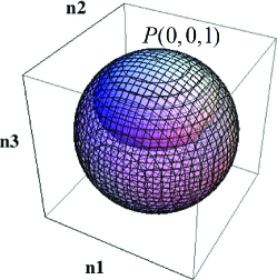
Figure 1: Qubits in Bloch representation undergoing the amplitude-damping channel. For the channel, $p=0.1$. The outer ball represents all the states of a qubit. The inner spheriod denotes the states that loses coherence via the channel. The two balls inscribe at point $P=(0,0,1)$

IV.2 Quantum channels on subsystems: disentangling factor

Since the direct consideration of decoherence of mixed state could lead to the confusion, we have to consider the mixed states in an indirect way, namely, we turn to an entangled bipartite composite system of a pure state with one of its subsystems undergoing a quantum channel. It is obvious that the reduced density matrix of any subsystem is mixed; In addition, any local quantum channel on the subsystem will always reduce the entanglement of the composite system since a good entanglement measure should be an entanglement monotone. However, it should be noted that the decoherence based on disentanglement is different from our initial definition 1. Strictly speaking, we actually characterize the reduction of a special coherence——quantum entanglement. In this sense, what we consider should be called as the disentangling power instead of the decoherence power of the original definition 1.

Consider a bipartite pure state of two qubits $\rho_{AB}$, the entanglement can be reduced if one subsystem undergoes a quantum channel $\$$. If we employ concurrence [32] as entanglement measure, one can easily find that [33]

$$C(\$\left(\rho_{AB}\right))=C(\$\left(\rho_{\Phi}\right))C(\rho_{AB}),$$

with $\rho_{\Phi}=\left|\Phi_{2}\right\rangle\left\langle\Phi_{2}\right|$. So no matter what distribution of quantum states is considered, the concurrence is directly reduced by the factor $C(\$\left(\rho_{\Phi}\right))$. Thus the disentangling power of $\$$ in this case can be directly characterized by $C(\$\left(\rho_{\Phi}\right))$.

In addition, if $\rho_{AB}$ is a mixed state, one can also consider the reduction of entanglement subject to some quantum channel. However, due to the complicated expression of concurrence for mixed states. So far there has not such a factorial form of the reduction of entanglement.

V Conclusions

In this paper, we study how a quantum channel influences the fidelity and the coherence of a state when the state goes through it and briefly discuss the reduction of entanglement when a subsystem undergoes a channel. We give the infidelity power and decoherence power of a quantum channel. They are independent of quantum states and describe an average contribution of the infidelity and the decoherence. As applications, we calculate the infidelity power and decoherence power of depolarizing channel, phase-damping channel, amplitude-damping channel and generalized amplitude-damping channel, respectively. We show that although quantum channels (if it is not trivial) definitely reduce the fidelity of the state through it and the entanglement with subsystems through it, for some channels, they could increase the coherence of some states.

VI Acknowledgements

This work was supported by the National Natural Science Foundation of China, under Grant No. 11175033 and the Fundamental Research Funds of the Central Universities, under Grant No. DUT12LK42.

References

• (1) R. Horodecki, P. Horodecki, M. Horodecki, and K. Horodecki, Rev. Mod. Phys. 81, 865 (2009).
• (2) L. Henderson, and V. Vedral, J. Phys. A 34, 6899 (2001).
• (3) V. Vedral, Phys. Rev. Lett. 90, 050401 (2003).
• (4) H. Ollivier, and W. H. Zurek, Phys. Rev. Lett. 88, 017901(2001).
• (5) Chang-shui Yu, Jia-sen Jin, Heng Fan, He-shan Song, Phys. Rev. A 87, 022113 (2013).
• (6) T. Werlang, S. Souza, F. F. Fanchini, and C. J. VillasBoas, Phys. Rev. A, 80, 024103 (2009); F. F. Fanchini, T. Werlang, C. A. Brasil, L.Β G. E. Arruda, and A. O. Caldeira, ibid., 81, 052107 (2010); J. Maziero, L.C. Celeri, R. M. Serra, and V. Vedral, ibid., 80, 044102 (2009); A. Ferraro, L. Aolita, D. Cavalcanti, F. M. Cucchietti, and A. Acin, ibid., 81, 052318 (2010).
• (7) B. Dakic, V. Vedral, and C. Brukner, Phys. Rev. Lett. 105, 190502 (2010).
• (8) Chang-shui Yu, and Haiqing Zhao, Phys. Rev. A 84, 062123 (2011) .
• (9) D. Cavalcanti, L. Aolita, S. Boixo, K. Modi, M. Piani, and A. Winter, Phys. Rev. A 83, 032324 (2011).
• (10) M. Piani, S. Gharibian, G. Adesso, J. Calsamiglia, P. Horodecki, and A. Winter, Phys. Rev. Lett. 106, 220403 (2011).
• (11) Chang-shui Yu, and He-shan Song, Phys. Rev. A 80, 022324 (2009).
• (12) Chang-shui Yu, Yang Zhang and Haiqing Zhao, unpublished.
• (13) W. H. Zurek, Rev. Mod. Phys. 75, 715 (2003).
• (14) M. Schlosshauer, Rev. Mod. Phys. 76, 1267 (2005).
• (15) A. J. Berkley, H. Xu, M. A. Gubrud, R. C. Ramos, J. R. Anderson, C. J. Lobb, and F. C. Wellstood, Phys. Rev. B 68, 060502 (2003).
• (16) Alessandro Romito, Francesco Plastina, and Rosario Fazio, Phys. Rev. B 68, 140502 (2003).
• (17) T. HakioΗ§lu and Kerim Savran, Phys. Rev. B 71, 115115 (2005).
• (18) J. Bergli, Y. M. Galperin, and B. L. Altshuler, Phys. Rev. B 74, 024509 (2006).
• (19) P. R. Eastham, A. O. Sprachlen, and J. Keeling, Phys. Rev. B 87, 195306 (2013).
• (20) Masahide Sasaki, Atsushi Hasegawa, Junko Ishi-Hayase, Yasuyoshi Mitsumori, and Fujio Minami, Phys. Rev. B 71, 165314 (2005).
• (21) J. Q. You, Xuedong Hu, and Franco Nori, Phys. Rev. B Β 72, 144529 (2005).
• (22) T. Vanderbruggen, R. Kohlhaas, A. Bertoldi, S. Bernon, A. Aspect, A. Landragin, and P. Bouyer, Phys. Rev. Lett. 110, 210503 (2013).
• (23) M. Al-Amri, Gao-xiang Li, Rong Tan, and M. Suhail Zubairy, Phys. Rev. A 80, 022314 (2009).
• (24) T. Yu and J. H. Eberly, Phys. Rev. B 68, 165322 (2003).
• (25) T. Yu and J. H. Eberly, Phys. Rev. Lett. 97, 140403 (2006).
• (26) T. Yu and J. H. Eberly Phys. Rev. Lett. 97, 140403 (2006).
• (27) Paolo Zanardi, Christof Zalka, and Lara Faoro, Phys. Rev. A 62, 030301 (2000).
• (28) L. Clarisse, S. Ghosh, S. Severini, and A. Sudbery, Phys. Letts. A 365, 400 (2007).
• (29) Michael A. Nielsen, Isaac L. Chuang, Quantum Computation and Quantum information, Cambridge University Press, 2010.
• (30) Robert Alicki, Marco Piani and Nicholas Van Ryn, J. Phys. A: Math. Theor. 41, 495303 (2008).
• (31) Chang-shui Yu, Jun Zhang and Heng Fan, Phys. Rev. A 82, 052317 (2012).
• (32) W. K. Wootters, Phys. Rev. Lett. 80, 2245 (1998).
• (33) T. Konrad, F. Melo, M. Tiersch, C. Kasztelan, A. Aragao and A. Buchleitner. Nature physics 4, 99 (2008).