Discrete bright solitons in Bose-Einstein condensates
and dimensional reduction in quantum field theory

Abstract

We first review the derivation of an effective one-dimensional (1D) discrete nonpolynomial Schrödinger equation from the continuous 3D Gross-Pitaevskii equation with transverse harmonic confinement and axial periodic potential. Then we study the bright solitons obtained from this discrete nonpolynomial equation showing that they give rise to the collapse of the condensate above a critical attractive strength. We also investigate the dimensional reduction of a bosonic quantum field theory, deriving an effective 1D nonpolynomial Heisenberg equation from the 3D Heisenberg equation of the continuous bosonic field operator under the action of transverse harmonic confinement. Moreover, by taking into account the presence of an axial periodic potential we find a generalized Bose-Hubbard model which reduces to the familiar 1D Bose-Hubbard Hamiltonian only if a strong inequality is satisfied. Remarkably, in the absence of axial periodic potential our 1D nonpolynomial Heisenberg equation gives the generalized Lieb-Liniger theory we obtained some years ago.

I Introduction

Ultracold bosonic gases in reduced dimensionality are an ideal platform for probing many-body phenomena  giamarchi ; cazalilla2011 . In particular, the use of optical lattices has allowed the experimental realization bloch of the well-known Bose-Hubbard Hamiltonian book-lattice with dilute and ultracold alkali-metal atoms. This achievement has been of tremendous impact on several communities book-lattice , and in particular on theoreticians and mathematicians working with discrete nonlinear Schrödinger equations kevre .

The three-dimensional (3D) Gross-Pitaevskii equation, a cubic nonlinear Schrödinger equations which accurately describes a Bose-Einstein condensate (BEC) made of dilute and ultracold atoms book-bose , is usually analyzed in the case of repulsive interaction strength which corresponds to a positive inter-atomic s-wave scattering length bloch_review . Indeed, a negative s-wave scattering length implies an attractive interaction strength which may bring to the collapse book-bose due to the shrink of the transverse width of a realistic quasi-1D bosonic cloud sala-npse ; sala-dnpse1 ; sala-dnpse2 . Nevertheless, in certain regimes of interaction both continuous and discrete 3D Gross-Pitaevskii equations predict the existence of meta-stable configurations which are usually called continuous and discrete bright solitons sala-npse ; sala-dnpse1 ; sala-dnpse2 . We remark that continuous bright solitons have been observed in various experiments exp-solo1 ; exp-solo2 ; exp-solo3 ; exp-solo4 involving attractive bosons of ⁷Li and ⁸⁵Rb vapors. Instead, discrete (gap) bright solitons in quasi-1D optical lattices have been observed exp-gap only with repulsive bosons made of ⁸⁷Rb atoms.

In the first part we discuss an effective one-dimensional discrete nonpolynomial Schrödinger equation obtained from the continuous 3D Gross-Pitaevskii equation with transverse harmonic confinement and axial periodic potential sala-dnpse1 ; sala-dnpse2 . We show that this 1D discrete nonpolynomial Schrödinger equation reduces to the 1D discrete Gross-Pitaevskii equation only in the weak-coupling regime and we compare the bright soliton of the discrete nonpolynomial Schrödinger equation bright solitons with the bright solitons of the discrete Gross-Pitaevskii equation.

In the second part, we investigate the dimensional reduction of a bosonic quantum field theory, deriving an effective 1D nonpolynomial Heisenberg equation from the 3D Heisenberg equation of the bosonic field operator under the action of transverse harmonic confinement. In particular, we prove that the discrete version of this 1D nonpolynomial Heisenberg equation becomes the 1D discrete nonpolynomial Schrödinger equation only assuming that the quantum many-body state of the system is a Glauber coherent state. As a by-product, we also obtain a reliable generalizaton of the Lieb-Liniger theory for a quasi-1D uniform Bose gas sala-lieb1 .

It is important to stress that some years ago we used this generalized Lieb-Liniger theory (but in the absence of axial lattice) to analyze the transition from a 3D Bose-Einstein condensate to the 1D Tonks-Girardeau gas, showing that the sound velocity and the frequency of the lowest compressional mode give a clear signature of the regime involved sala-lieb1 . In Ref. sala-lieb1 we studied also the case of negative scattering length deriving the phase diagram of the Bose gas (uniform, single soliton, multi soliton and collapsed) in toroidal confinement. Quite remarkably, the experimental data on a Tonks-Girardeau gas of ⁸⁷Rb atoms of Kinoshita, Wenger, and Weiss kinoshita are compatible with the one-dimensional theory of Lieb, Seiringer and Yngvason lieb but are better described by our theory that takes into account variations in the transverse width of the atomic cloud sala-lieb2 . In Ref. sala-lieb2 , by using our generalized theory we investigated also the free axial expansion of the ⁸⁷Rb gas in different regimes: Tonks-Girardeau gas, one-dimensional Bose-Einstein condensate and three-dimensional Bose-Einstein condensate.

II BEC in a quasi-1D optical lattice

We consider a dilute BEC confined in the $z$ direction by a generic axial potential $V(z)$ and in the plane $(x,y)$ by the transverse harmonic potential

$$U(x,y)={m\over 2}\omega_{\bot}^{2}\left(x^{2}+y^{2}\right)\;.$$ (1)

The characteristic harmonic length is given by

$$a_{\bot}=\sqrt{\hbar\over m\omega_{\bot}}\;,$$ (2)

and, for simplicity, we choose $a_{\bot}$ and $\omega_{\bot}^{-1}$, as length and time units, and $\hbar\omega_{\bot}$ as energy unit. In the remaining part of this chapter we use non-dimensional variabiles.

We assume that the system made of fully condensed Bose atoms is well described by the 3D Gross-Pitaevskii equation, and in scaled units it reads

$$i{\frac{\partial}{\partial t}}\psi(\mathbf{r},t) = \Big{[}-{\frac{1}{2}}\nabla^{2}+{1\over 2}\left(x^{2}+y^{2}\right)+V(z)$$ (3)

$$+ 2\pi g|\psi(\mathbf{r},t)|^{2}\Big{]}\psi(\mathbf{r},t)\;,$$

where $\psi(\mathbf{r},t)$ is the macroscopic wave function of the BEC normalized to the total number $N$ of atoms and $g=2a_{s}/a_{\bot}$ with $a_{s}$ the s-wave scattering length of the inter-atomic potential. In addition, we suppose that the axial potential is the combination of periodic and harmonic potentials, i.e.

$$V(z)=V_{0}\cos{(2kz)}+{1\over 2}\lambda^{2}z^{2}\;.$$ (4)

This potential models the quasi-1D optical lattice produced in experiments with Bose-Einstein condensates by using counter-propagating laser beams morsch . Here $\lambda\ll 1$ models a weak axial harmonic confinement.

II.1 Axial discretization of the 3D Gross-Pitaevskii equation

We now perform a discretization of the 3D Gross-Pitaevskii equation along the $z$ axis due to the presence on the periodic potential. In particular we set

$$\psi(\mathbf{r},t)=\sum_{n}\phi_{n}(x,y,t)\ W_{n}(z)\;,$$ (5)

where $W_{n}(z)$ is the Wannier function maximally localized at the $n$-th minimum of the axial periodic potential. This tight-binding ansatz is reliable in the case of a deep optical lattice morsch .

We insert this ansatz into Eq. (3), multiply the resulting equation by $W_{n}^{*}(z)$ and integrate over $z$ variable. In this way we get

$$i{\partial\over\partial t}\phi_{n} = \Big{[}-\frac{1}{2}\nabla_{\bot}^{2}+\frac{1}{2}\left(x^{2}+y^{2}\right)+\epsilon_{n}\Big{]}\phi_{n}$$ (6)

$$- J\left(\phi_{n+1}+\phi_{n-1}\right)+2\pi U\left|\phi_{n}\right|^{2}\phi_{n}\>,$$

where the parameters $\epsilon$, $J$ and $U$ are given by

$$\epsilon_{n}=\int W_{n}^{*}(z)\left[-{1\over 2}{\partial^{2}\over\partial z^{2}}+V(z)\right]W_{n}(z)\ dz\;,$$ (7)

$$J=-\int W_{n+1}^{*}(z)\left[-{1\over 2}{\partial^{2}\over\partial z^{2}}+V(z)\right]W_{n}(z)\ dz\;,$$ (8)

$$U=g\int|W_{n}(z)|^{4}\ dz\;.$$ (9)

The parameters $J$ and $U$ are practically independent on the site index $n$ and in the tight-binding regime $J>0$.

II.2 Transverse dimensional reduction of the 3D discrete Gross-Pitaevskii equation

To further simplify the problem we set sala-dnpse1 ; sala-dnpse2

$$\phi_{n}(x,y)={1\over\pi^{1/2}\sigma_{n}(t)}\exp{\left[-\left({x^{2}+y^{2}\over 2\sigma_{n}(t)^{2}}\right)\right]}\,f_{n}(t)\;,$$ (10)

where $\sigma_{n}(t)$ and $f_{n}(t)$, which account for discrete transverse width and discrete axial wave function, are the effective generalized coordinates to be determined variationally. In Ref. sala-gaussian there is a detailed discussion of the variational approach with time-dependent Gaussian trial wave-functions for the study of Bose-Einstein condensates.

We insert this ansatz into the Lagrangian density associated to Eq. (6) and integrate over $x$ and $y$ variables. In this way we obtain an effective Lagrangian for the fields $f_{n}(t)$ and $\sigma_{n}(t)$.

The Euler-Lagrange equation of the effective Lagrangian with respect to $f_{n}^{*}$ is

$$i{\partial\over\partial t}f_{n} = \left[{1\over 2}\left({1\over\sigma_{n}^{2}}+\sigma_{n}^{2}\right)+\epsilon_{n}\right]f_{n}-J\,\left(f_{n+1}+f_{n-1}\right)$$ (11)

$$+ {U\over\sigma_{n}^{2}}|f_{n}|^{2}f_{n}\;.$$

while the Euler-Lagrange equation with respect to $\sigma_{n}$ gives

$$\sigma_{n}^{4}=1+U|f_{n}|^{2}\;.$$ (12)

Inserting Eq. (12) into Eq. (11) we finally get

$$i{\partial\over\partial t}f_{n}=\epsilon_{n}\,f_{n}-J\,\left(f_{n+1}+f_{n-1}\right)+\frac{1+{(3/2)}U|f_{n}|^{2}}{\sqrt{1+U|f_{n}|^{2}}}f_{n}\;,$$ (13)

that is the 1D discrete nonpolynomial Schrödinger equation, describing the BEC under a transverse anisotropic harmonic confinement and an axial optical lattice sala-dnpse1 ; sala-dnpse2 .

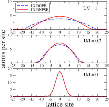
Figure 1: Weakly repulsive bosons in the optical lattice. Axial density profile (atoms per site) of $N=100$ repulsive bosonic atoms in a optical lattice with a super-imposed harmonic potential ($\lambda=0.1$). The three panels correspond (from bottom to top) to increasing values of the adimensional on-site interaction strength $U/J:0,0.2,1$. Solid lines: results obtained by using the 1D discrete nonpolynomial Schrodinger equation (DNPSE); dashed lines: results obtained by using the 1D discrete Gross-Pitaevskii equation (DGPE). In the lower panel ($U/J=0$) the two curves are superimposed.

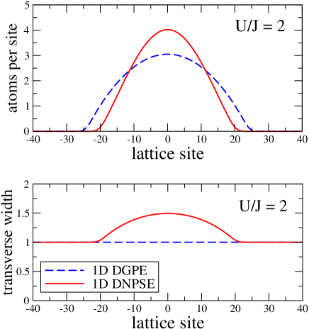
Figure 2: Strongly repulsive bosons in the optical lattice ($U/J=2$). Upper panel: Axial density profile (atoms per site) of $N=100$ repulsive bosonic atoms in a optical lattice with a super-imposed harmonic potential ($\lambda=0.1$). Lower panel: the transverse width of the bosonic cloud. Solid lines: results obtained by using the 1D discrete nonpolynomial Schrodinger equation (DNPSE); dashed lines: results obtained by using the 1D discrete Gross-Pitaevskii equation (DGPE).

The 1D discrete nonpolynomial Schrödinger equation reduces to the familiar 1D discrete Gross-Pitaevskii equation

$$i{\partial\over\partial t}f_{n}=\epsilon_{n}\,f_{n}-J\,\left(f_{n+1}+f_{n-1}\right)+U|f_{n}|^{2}f_{n}\;$$ (14)

in the weak-coupling limit $|U||f_{n}|^{2}\ll 1$, where $U$ can be both positive and negative. On the contrary, 1D discrete nonpolynomial Schrödinger equation becomes a 1D quadratic discrete nonlinear Schrödinger equation

$$i{\partial\over\partial t}f_{n}=\epsilon_{n}\,f_{n}-J\,\left(f_{n+1}+f_{n-1}\right)+(3/2)\sqrt{U}|f_{n}|f_{n}\;$$ (15)

in the strong-coupling limit $U|f_{n}|^{2}\gg 1$, where $U>0$.

II.3 Numerical results

We have solved numerically both 1D discrete nonpolynomial Schrödinger equation and 1D discrete Gross-Pitaevskii equation by using a Crank-Nicolson predictor-corrector algorithm with imaginary time sala-numerics to get the ground-state of the system.

In Fig. 1 and 2 we report our results obtained with $N=100$ atoms in a quasi-1D optical lattice with weak axial harmonic confinement: $\lambda=0.1$. The plots are shown for different values of the repulsive on-site interaction strength $U$: $U>0$. Note that in the experiments $U$ can be tuned by using the technique of Feshbach resonances book-lattice ; book-bose ; morsch .

In Fig. 1 we plot the axial density profile $|f_{n}|^{2}$ of weakly repulsive bosons in a optical lattice with a super-imposed harmonic potential. As described in the caption, the three panels correspond (from bottom to top) to increasing values of the on-site interation strength $U$. Fig. 1 clearly shows that the results (solid lines) obtained by using the 1D discrete nonpolynomial Schrodinger equation strongly differ with respect to the ones (dashed lines) obtained by using the 1D discrete Gross-Pitaevskii equation by increasing the on-site interaction. This effect is better shown in the upper panel of Fig. 2, where we plot the axial density profile for a large value ($U/J=2$) of the on-site interaction. In the lower panel of Fig. 2 we report the transverse width $\sigma_{i}$ of the bosonic cloud as a function of the lattice site $n$. As expected, $\sigma_{i}$ strongly deviates from $1$ (i.e. $a_{\bot}$ is dimensional units) where the axial density $|f_{n}|^{2}$ is large.

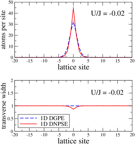
Figure 3: Weakly attractive bosons in the optical lattice ($U/J=-0.02$). Upper panel: Axial density profile (atoms per site) of $N=100$ attractive bosonic atoms in a optical lattice with a super-imposed harmonic potential ($\lambda=0.1$). Lower panel: the transverse width of the bosonic cloud. Solid lines: results obtained by using the 1D discrete nonpolynomial Schrodinger equation (DNPSE); dashed lines: results obtained by using the 1D discrete Gross-Pitaevskii equation (DGPE).

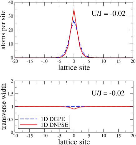
Figure 4: Weakly attractive bosons in the optical lattice ($U/J=-0.02$) without the super-imposed harmonic confinement ($\lambda=0$). Upper panel: Axial density profile (atoms per site) of $N=100$ attractive bosonic atoms in a optical lattice. Lower panel: the transverse width of the bosonic cloud. Solid lines: results obtained by using the 1D discrete nonpolynomial Schrodinger equation (DNPSE); dashed lines: results obtained by using the 1D discrete Gross-Pitaevskii equation (DGPE).

Now we show the results obtained again with $N=100$ atoms in a quasi-1D optical lattice but with an attractive on-site interaction strength $U$: $U<0$. In the attractive case the ground-state is self-localized and it exists also in the absence ($\lambda=0$) of the axial harmonic potential: it is the discrete bright soliton. In Fig. 3 we plot the axial density profile $|f_{n}|^{2}$ in the presence of the super-imposed axial harmonic potential ($\lambda=0.1$) and in Fig. 4 in the absence of the super-imposed axial harmonic potential ($\lambda=0$) choosing $U/J=-0.02$. The two figures show that that the density profiles with and without axial harmonic potential are practically the same. In the figures there is also the comparison between 1D nonpolynomial Schrödinger equation (solid lines) and 1D Gross-PItaevskii equation (dashed lines).

II.4 Collapse of the discrete bright soliton

In Fig. 5 we report the axial width of the bright soliton as a fuction of the (attractive) on-site interaction. As expected, for a small on-site interaction strength the axial width is extremely large and 1D discrete nonpolynomial Schrödinger equation and 1D discrete Gross-Pitaevskii equation give the same results. On the other hand, if the on-site interaction strength is sufficiently large one finds deviations between 1D discrete nonpolynomial Schrödinger equation and 1D discrete Gross-Pitaevskii equation. By further increasing the attractive on-site interaction $U$ 1D discrete Gross-Pitaevskii equation shows that eventually all the atoms accumulate into the same site. 1D discrete nonpolynomial Schrödinger equation shows instead something different: before all the atoms populate the same site there is the collapse of the condensate: 1D discrete nonpolynomial Schrödinger equation does not admit anymore a finite ground-state solution.

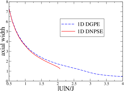
Figure 5: Weakly attractive bosons in the optical lattice without the super-imposed harmonic confinement ($\lambda=0$). Transverse width of the bosonic cloud of $N=100$ atoms as a function of the effective interaction strength $|U|N/J$. Solid lines: results obtained by using the 1D discrete nonpolynomial Schrodinger equation (DNPSE); dashed lines: results obtained by using the 1D discrete Gross-Pitaevskii equation (DGPE).

Numerically we find that the collapse occurs when $U<0$ and

$${|U|N\over J}>2.1$$ (16)

which is consistent with analytical result ${|U|N/J}>8/3$ of the continuum limit sala-npse .

III Dimensional reduction of a continuous quantum field theory

A full quantum treatment of interacting bosons in a optical lattice is obtained by promoting the wavefunction $\psi({\bf r},t)$ of the 3D Gross-Pitaevskii equation (3) to a field operator ${\hat{\psi}}({\bf r},t)$ sala-book , namely

$$\psi(\mathbf{r},t)\to{\hat{\psi}}(\mathbf{r},t)\;,$$ (17)

$$\psi^{*}(\mathbf{r},t)\to{\hat{\psi}}^{+}(\mathbf{r},t)\;.$$ (18)

The bosonic field operator ${\hat{\psi}}({\bf r},t)$ and its adjunct ${\hat{\psi}}^{+}({\bf r},t)$ must satisfy the following equal-time commutation rules

$$[{\hat{\psi}}({\bf r},t),{\hat{\psi}}^{+}({\bf r}^{\prime},t)]=\delta({\bf r}-{\bf r}^{\prime})\;,$$ (19)

$$[{\hat{\psi}}({\bf r},t),{\hat{\psi}}({\bf r}^{\prime},t)]=[{\hat{\psi}}^{+}({\bf r},t),{\hat{\psi}}^{+}({\bf r}^{\prime},t)]=0\;,$$ (20)

By imposing these commutation rules one finds

$${\hat{\psi}}^{+}({\bf r},t)|0\rangle=|{\bf r},t\rangle\;,$$ (21)

that is the operator ${\hat{\psi}}^{+}({\bf r},t)$ creates a particle in the state $|{\bf r},t\rangle$ from the vacuum state $|0\rangle$, and also

$${\hat{\psi}}({\bf r},t)|{\bf r}^{\prime}t\rangle=\delta({\bf r}-{\bf r}^{\prime})\ |0\rangle\;,$$ (22)

that is the operator ${\hat{\psi}}({\bf r},t)$ annihilates a particle which is in the state $|{\bf r},t\rangle$.

After promoting the wavefunction $\psi(\mathbf{r},t)$ to a field operator ${\hat{\psi}}(\mathbf{r},t)$, Eq. (3) becomes

$$i{\frac{\partial}{\partial t}}{\hat{\psi}}(\mathbf{r},t) = \Big{[}-{\frac{1}{2}}\nabla^{2}+{1\over 2}\left(x^{2}+y^{2}\right)+V(z)$$ (23)

$$+ 2\pi g{\hat{\psi}}^{+}(\mathbf{r},t){\hat{\psi}}(\mathbf{r},t)\Big{]}{\hat{\psi}}(\mathbf{r},t)\;,$$

This equation is nothing else than the Heisenberg equation of motion

$$i{\partial\over\partial t}{\hat{\psi}}=[{\hat{\psi}},{\hat{H}}]\;$$ (24)

of the field operator ${\hat{\psi}}(\mathbf{r},t)$, where

$${\hat{H}}=\int d^{3}{\bf r}\ {\hat{\psi}}^{+}\left[-{\frac{1}{2}}\nabla^{2}+{1\over 2}\left(x^{2}+y^{2}\right)+V(z)+2\pi g{\hat{\psi}}^{+}{\hat{\psi}}\right]{\hat{\psi}}$$ (25)

is the many-body quantum Hamiltonian of the system, which is not necessarily a BEC sala-book . Thus, the many-body Hamiltonian (25) describes a dilute gas of bosonic atoms confined in the plane $(x,y)$ by the transverse harmonic potential and by a generic potential $V(z)$ in the $z$ direction.

III.1 Dimensional reduction of the Hamiltonian

To perform the dimensional reduction of the Hamiltonian (25) we suppose that

$${\hat{\psi}}({\bf r})|G\rangle={1\over\pi^{1/2}\sigma(z)}\exp{\left[-\left({x^{2}+y^{2}\over 2\sigma(z)^{2}}\right)\right]}\,{\hat{\phi}}(z)|G\rangle\;,$$ (26)

where $|G\rangle$ is the many-body ground state, while $\sigma(z)$ and ${\hat{\phi}}(z)$ account respectively for the transverse width and for the axial bosonic field operator. We apply this ansatz to Eq. (25) and obtain

$${\hat{H}}|G\rangle={\hat{H}}_{e}|G\rangle$$ (27)

where, neglecting the space derivatives of $\sigma(z)$, the effective 1D Hamiltonian reads

$${\hat{H}}_{e}=\int dz\ {\hat{\phi}}^{+}\Big{[}-{\frac{1}{2}}\partial_{z}^{2}+V(z)+{1\over 2}\left({1\over\sigma^{2}}+\sigma^{2}\right)+{g\over 2\sigma^{2}}\ {\hat{\phi}}^{+}{\hat{\phi}}\Big{]}{\hat{\phi}}\;.$$ (28)

The transverse width $\sigma(z)$ can be determined by averaging the Hamiltonian (28) over the ground state $|G\rangle$ and minimizing the resulting energy functional

$$\langle G|{\hat{H}}_{e}|G\rangle = \int dz\Big{\{}\langle G|{\hat{\phi}}^{+}\Big{[}-{\frac{1}{2}}\partial_{z}^{2}+V(z)\Big{]}{\hat{\phi}}|G\rangle$$ (29)

$$+ {1\over 2}\left({1\over\sigma^{2}}+\sigma^{2}\right)\langle G|{\hat{\phi}}^{+}{\hat{\phi}}|G\rangle$$

$$+ {g\over 2\sigma^{2}}\langle G|{\hat{\phi}}^{+}{\hat{\phi}}^{+}{\hat{\phi}}{\hat{\phi}}|G\rangle\Big{\}}$$

with respect to $\sigma(z)$. In this way one gets

$$\sigma(z)^{4}=1+g{\langle G|{\hat{\phi}}^{+}(z){\hat{\phi}}^{+}(z){\hat{\phi}}(z){\hat{\phi}}(z)|G\rangle\over\langle G|{\hat{\phi}}^{+}(z){\hat{\phi}}(z)|G\rangle}\;.$$ (30)

Thus, the ground state $|G\rangle$ is obtained self-consistently from Eqs. (28) and (30). Notice that introducing the local axial-density operator ${\hat{\rho}}(z)={\hat{\phi}}^{+}(z){\hat{\phi}}(z)$, such that $\rho(z)=\langle G|{\hat{\phi}}^{+}(z){\hat{\phi}}(z)|G\rangle=\langle G|{\hat{\rho}}(z)|G\rangle$ is the local axial density and $\rho_{2}(z)=\langle G|{\hat{\phi}}^{+}(z){\hat{\phi}}^{+}(z){\hat{\phi}}(z){\hat{\phi}}(z)=\langle G|{\hat{\rho}}(z){\hat{\rho}}(z)|G\rangle-\delta(0)\,\rho(z)$ is the two-body axial correlation function, Eq. (30) can be rewritten as

$$\sigma(z)^{4}=1+g{\rho_{2}(z)\over\rho(z)}\;.$$ (31)

Clearly, if $g\rho_{2}(z)\ll\rho(z)$ one has

$$\sigma=1$$ (32)

and the effective Hamiltonian (28) reduces to

$${\hat{H}}_{e}={\hat{H}}_{1D}+1\;,$$ (33)

where ${\hat{H}}_{1D}$ is the strictly one-dimensional Hamiltonian

$${\hat{H}}_{1D}=\int dz\ {\hat{\phi}}^{+}\Big{[}-{\frac{1}{2}}\partial_{z}^{2}+V(z)+{g\over 2}\ {\hat{\phi}}^{+}{\hat{\phi}}\Big{]}{\hat{\phi}}\;$$ (34)

while $1$ is the transverse energy (in units of $\hbar\omega_{\bot}$).

Let us analyze the general case $\sigma(z)\neq 1$. In the superfluid regime, where $|G\rangle$ is the Glauber coherent state $|GCS\rangle$ of ${\hat{\phi}}(z)$ sala-book , i.e. such that

$${\hat{\phi}}(z)|GCS\rangle=\phi(z)|GCS\rangle\;,$$ (35)

from Eq. (30) one finds

$$\sigma(z)^{4}=1+g|\phi(z)|^{2}\;$$ (36)

and the energy functional (29) then becomes

$$\langle GCS|{\hat{H}}_{e}|GCS\rangle=\int dz\ \phi^{*}\Big{[}-{1\over 2}\partial_{z}^{2}+V(z)+\sqrt{1+g|\phi|^{2}}\Big{]}\phi\;.$$ (37)

This is the familiar energy functional of the 1D nonpolynomial Schrödinger equation sala-npse .

III.2 1D nonpolynomial Heisenberg equation

From the effective 1D Hamiltonian (28), the Heisenberg equation of motion

$$i{\partial\over\partial t}{\hat{\phi}}=[{\hat{\phi}},{\hat{H}}_{e}]\;$$ (38)

gives

$$i{\partial\over\partial t}{\hat{\phi}}(z,t) = \Big{[}-{\frac{1}{2}}\partial_{z}^{2}+V(z)+{1\over 2}\left({1\over\sigma^{2}(z,t)}+\sigma^{2}(z,t)\right)$$ (39)

$$+ {g\over\sigma(z,t)^{2}}\ {\hat{\phi}}^{+}(z,t){\hat{\phi}}(z,t)\Big{]}{\hat{\phi}}(z,t)\;,$$

that is a 1D nonpolynomial Heisenberg equation because it must be solved self-consistently with the equation

$$\sigma(z,t)^{4}=1+g{\langle S|{\hat{\phi}}^{+}(z,t){\hat{\phi}}^{+}(z,t){\hat{\phi}}(z,t){\hat{\phi}}(z,t)|S\rangle\over\langle S|{\hat{\phi}}^{+}(z,t){\hat{\phi}}(z,t)|S\rangle}\;,$$ (40)

where $|S\rangle$ is the many-body quantum state on the system. Only if the many-body state $|S\rangle$ coincides with the Glauber coherent state $|GCS\rangle$ sala-book , such that ${\hat{\phi}}(z,t)|GCS\rangle=\phi(z,t)|GCS\rangle$, the 1D nonpolynomial Heisenberg equation reduces to the 1D nonpolynomial Schrodinger equation sala-npse , given by

$$i{\partial\over\partial t}\phi(z,t) = \Big{[}-{\frac{1}{2}}\partial_{z}^{2}+V(z)+{1\over 2}\left({1\over\sigma^{2}(z,t)}+\sigma^{2}(z,t)\right)$$ (41)

$$+ {g\over\sigma(z,t)^{2}}\ |\phi(z,t)|^{2}\Big{]}\phi(z,t)\;,$$

where $\phi(z,t)$ is a complex wavefunction and

$$\sigma(z,t)=\left(1+g|\phi(z,t)|^{2}\right)^{1/4}\;$$ (42)

is the corresponding transverse width.

III.3 Generalized Lieb-Liniger theory

In the time-independent and uniform case, where $V(z)=0$, the space-time dependence in Eq. (40) disappears, i.e.

$$\sigma^{4}=1+g{\rho_{2}\over\rho}\;,$$ (43)

and the energy functional (29) reduces to a function of $\rho$, $\rho_{2}$ and $\sigma$, namely

$$\langle G|{{\hat{H}}_{e}\over L}|G\rangle=\langle G|{\hat{\phi}}^{+}\Big{[}-{\frac{1}{2}}\partial_{z}^{2}\Big{]}{\hat{\phi}}|G\rangle+{g\over 2\sigma^{2}}\rho_{2}+{1\over 2}\left({1\over\sigma^{2}}+\sigma^{2}\right)\rho\;,$$ (44)

where $L$ is the length of the uniform system. Due to the Lieb-Liniger theorem lieb , for $g\geq 0$ the energy function (44) can be rewritten as

$$\langle G|{{\hat{H}}_{e}\over L}|G\rangle={1\over 2}\rho^{3}f({g\over\rho\sigma^{2}})+{1\over 2}\left({1\over\sigma^{2}}+\sigma^{2}\right)\rho\;,$$ (45)

where $f(x)$ is the Lieb-Liniger function, which is defined as the solution of a Fredholm equation and it is such that $f(x)=x-4x^{3/2}/(3\pi)$ for $x\ll 1$ and $f(x)=(\pi^{2}/3)(x/(x+2))^{2}$ for $x\gg 1$. The minimization of (45) with respect to $\sigma$ gives

$$\sigma^{4}=1+g\rho\ f^{\prime}({g\over\rho\sigma^{2}})\;,$$ (46)

and consequently, comparing with Eq. (43), the two-body axial correlation function $\rho_{2}$ must satisfy the equation

$$\rho_{2}=\rho^{2}\ f^{\prime}({g\over\rho\sigma^{2}})\;.$$ (47)

Notice that Eqs. (45) and (46), which are a reliable generalization of the Lieb-Lineger theory, have been obtained for the first time by Salasnich, Parola and Reatto sala-lieb1 using a many-orbitals variational approach. As discussed in the introduction, some years ago we used this generalized Lieb-Liniger theory to analyze the transition from a 3D Bose-Einstein condensate to the 1D Tonks-Girardeau gas sala-lieb1 , showing that the experimental data on a Tonks-Girardeau gas of ⁸⁷Rb atoms of Kinoshita, Wenger, and Weiss kinoshita are very well described by our theory that takes into account variations in the transverse width of the atomic cloud sala-lieb2 .

IV Dimensional reduction for bosons in a quasi-1D lattice

To conclude this chapter, we perform a discretization of the 3D many-body Hamiltonian (25) along the $z$ axis due to the presence of the periodic potential, given by Eq. (4). We use the decomposition book-lattice

$${\hat{\psi}}(\mathbf{r})=\sum_{n}{\hat{\phi}}_{n}(x,y)\ W_{n}(z)\;,$$ (48)

that is the quantum-field-theory analog of Eq. (5) and we set up the quantum-field-theory extension of the mean-field approach developed in the first part of this contribution. In particular we write

$${\hat{\phi}}_{n}(x,y)|G\rangle={1\over\pi^{1/2}\sigma_{n}}\exp{\left[-\left({x^{2}+y^{2}\over 2\sigma_{n}^{2}}\right)\right]}\,{\hat{b}}_{n}|G\rangle\;,$$ (49)

where $|G\rangle$ is the many-body ground state, while $\sigma_{n}$ and ${\hat{b}}_{n}$ account respectively for the on-site transverse width and for the bosonic field operator. We insert these ansatz into Eq. (25) and we easily obtain the effective 1D Bose-Hubbard Hamiltonian sala-barba

$${\hat{H}}_{e} = \sum_{n}\Big{\{}\big{[}{1\over 2}({1\over\sigma_{n}^{2}}+\sigma_{n}^{2})+\epsilon_{n}\big{]}{\hat{n}}_{n}-J\,{\hat{b}}_{n}^{+}\left({\hat{b}}_{n+1}+{\hat{b}}_{n-1}\right)$$ (50)

$$+ {1\over 2}{U\over\sigma_{n}^{2}}{\hat{n}}_{n}({\hat{n}}_{n}-1)\Big{\}}\;.$$

where ${\hat{n}}_{n}={\hat{b}}_{n}^{+}{\hat{b}}_{n}$ is the on-site number operator, $\epsilon_{n}$ is the on-site axial energy, while $J$ and $U$ are the familiar hopping (tunneling) energy and on-site energy, given by Eqs. (7), (8) and (9).

Our Eq. (50) takes into account deviations with respect to the strictly 1D case due to the transverse width $\sigma_{n}$ of the bosonic field. This on-site transverse width $\sigma_{n}$ can be determined by averaging the Hamiltonian (50) over a many-body quantum state $|G\rangle$ and minimizing the resulting energy function with respect to $\sigma_{n}$. In this way one gets sala-barba

$$\sigma_{n}^{4}=1+U{\langle G|{\hat{n}}_{n}^{2}|G\rangle-\langle G|{\hat{n}}_{n}|G\rangle\over\langle G|{\hat{n}}_{n}|G\rangle}\;.$$ (51)

Note that Eqs. (50) and (51) must be solved self-consistently to obtain the ground-state of the system. Clearly, if $U<0$ the transverse width $\sigma_{n}$ is smaller than one (i.e. $\sigma_{n}<a_{\bot}$ in dimensional units) and the collapse happens when $\sigma_{n}$ goes to zero. At the critical strength $U_{c}$ of the collapse all particles are accumulated in few sites and consequently $U_{c}\simeq-1/N$.

We stress that, from Eq. (51), the system is strictly 1D only if the following strong inequality

$$U{\langle{\hat{n}}_{n}^{2}\rangle-\langle{\hat{n}}_{n}\rangle\over\langle{\hat{n}}_{n}\rangle}\ll 1$$ (52)

is satisfied for any $n$, such that $\sigma_{n}=1$ (i.e. $\sigma_{n}=a_{\bot}$ in dimensional units). Under the condition (52) the problem of collapse is fully avoided. In this strictly 1D regime where the effective Hamiltonian of Eq. (50) becomes (neglecting the irrelevant constant transverse energy)

$${\hat{H}}_{1D}=\sum_{n}\epsilon_{n}{\hat{n}}_{n}-J\sum_{n}{\hat{b}}_{n}^{+}\left({\hat{b}}_{n+1}+{\hat{b}}_{n-1}\right)+\frac{U}{2}\sum_{n}{\hat{n}}_{n}({\hat{n}}_{n}-1)$$ (53)

which is the familiar 1D Bose-Hubbard model book-lattice .

Given the generalized Bose-Hubbard Hamiltonian (50), the discrete Heisenberg equation of motion of the bosonic operator ${\hat{b}}_{n}$ reads

$$i{\partial\over\partial t}{\hat{b}}_{n}=[{\hat{b}}_{n},{\hat{H}}_{e}]\;,$$ (54)

that is

$$i{\partial\over\partial t}{\hat{b}}_{n}=\big{[}{1\over 2}({1\over\sigma_{n}^{2}}+\sigma_{n}^{2})+\epsilon_{n}\big{]}{\hat{b}}_{n}-J\,\left({\hat{b}}_{n+1}+{\hat{b}}_{n-1}\right)+{U\over\sigma_{n}^{2}}{\hat{n}}_{n}\ {\hat{b}}_{n}\;.$$ (55)

This is a 1D discrete nonpolynomial Heisenberg equation because it must be solved self-consistently with the equation

$$\sigma_{n}^{4}=1+U{\langle S|{\hat{n}}_{n}^{2}|S\rangle-\langle S|{\hat{n}}_{i}|S\rangle\over\langle S|{\hat{n}}_{n}|S\rangle}\;.$$ (56)

where $|S\rangle$ is the many-body quantum state on the system. Also in this discrete case, only if the many-body state $|S\rangle$ coincides with the Glauber coherent state $|GCS\rangle$, such that

$${\hat{b}}_{n}\ |GCS\rangle=f_{n}\ |GCS\rangle\;,$$ (57)

the 1D discrete nonpolynamial Heisenberg equation reduces to the 1D discrete nonpolynomial Schrödinger equation, given by Eqs. (11) and (12).

V Conclusions

We have investigated the discrete bright solitons of a quasi-one-dimensional Bose-Einstein condensate with axial periodic potential by using an effective one-dimensional discrete nonpolynomial Schrödinger equation sala-dnpse1 ; sala-dnpse2 . We have shown that, contrary to the familiar one-dimensional discrete nonlinear Schrödinger equation, our gives rise to the collapse of the condensate above a critical (attractive) strength, in agreement with experimental data. We have also analyzed the dimensional reduction of a bosonic quantum field theory finding an effective 1D quantum Hamiltionian (and a corresponding effective 1D nonpolynomial Heisenberg equation) which gives a generalized Lieb-Liniger theory in the absence of axial periodic potential sala-lieb1 ; sala-lieb2 and gives instead a generalized Bose-Hubbard model sala-barba in the presence of axial periodic potential. In Ref. sala-barba we have used the Density-Matrix-Renormalization-Group (DMRG) technique to study the bright solitons of the 1D Bose-Hubbard Hamiltonian finding that beyond-mean-field effects become relevant by increasing the attraction between bosons. In particular we have discover that, contrary to the MF predictions based on the discrete nonlinear Schrödinger equation, quantum bright solitons are not self-trapped sala-barba . In other words, we have found that with a small number $N$ of bosons the average of the quantum density profile, that is experimentally obtained with repeated measures of the atomic cloud, is not shape invariant. This remarkable effect can be explained by considering a quantum bright soliton as a MF bright soliton with a center of mass that is randomly distributed due to quantum fluctuations, which are suppressed only for large values of $N$ sala-barba .

References

- (1) Barbiero, L., Salasnich, L.: Quantum bright solitons in a quasi-one-dimensional optical lattice. Phys. Rev. A 89, 063605 (2014)
- (2) Bloch, I., Dalibard, J., Zwerger, W.: Many-body physics with ultracold gases. Rev. Mod. Phys. 80, 885 (2008)
- (3) Cazalilla, M.A., Citro, R., Giamarchi, T., Orignac, E., Rigol, M.: One dimensional Bosons: From Condensed Matter Systems to Ultracold Gases. Rev. Mod Phys. 83 1405 (2011)
- (4) Cerboneschi, E., Mannella, R., Arimondo, E., Salasnich, L.: Oscillation Frequencies for a Bose Condensate in a Triaxial Magnetic Trap. Phys. Lett. A 249, 495 (1998); Mazzarella, G., Salasnich, L.: Collapse of triaxial bright solitons in atomic Bose-Einstein condensates. Phys. Lett. A 373, 4434 (2009)
- (5) Cornish, S.L., Thompson, S.T., Wieman, C.E., Formation of bright matter-wave solitons during the collapse of attractive Bose-Einstein condensates. Phys. Rev. Lett. 96, 170401 (2006)
- (6) Eiermann, B., Anker, Th., Albiez, M., Taglieber, M., Treutlein, P., Marzlin, K.P., Oberthaler, M.K.: Bright Bose-Einstein Gap Solitons of Atoms with Repulsive Interaction. Phys. Rev. Lett. 92, 230401 (2004)
- (7) Giamarchi, T.: Quantum Physics in One Dimension. Oxford Univ. Press, Oxford (2004)
- (8) M. Greiner, O. Mandel, T. Esslinger, T Hänsch, and I. Bloch, Nature 415, 39 (2002).
- (9) Leggett, A.J.: Quantum Liquids. Bose condensation and Cooper Pairing in Condensed-Matter Systems. Oxford Univ. Press, Oxford (2006)
- (10) Lewenstein, M., Sanpera, A., Ahufinger, V.: Ultracold Atoms in Optical Lattices: Simulating Quantum Many-Body Systems. Oxford Univ. Press, Oxford (2012)
- (11) E.H. Lieb and W. Liniger, Exact Analysis of an Interacting Bose Gas. I. The General Solution and the Ground State. Phys. Rev. 130, 1605 (1963)
- (12) A. Maluckov, L. Hadzievski, B.A. Malomed, and L. Salasnich, Solitons in the discrete nonpolynomial Schrödinger equation. Phys. Rev. A 78, 013616 (2008)
- (13) G. Gligoric, A. Maluckov, L. Salasnich, B.A. Malomed, and L. Hadzievski, Two routes to the one-dimensional discrete nonpolynomial Schrd̈inger equation. Chaos 19, 043105 (2009)
- (14) Marchant, A.L., Billam, T.P., Wiles, T.P., Yu, M.M.H., Gardiner S.A., Cornish, S.L.: Controlled formation and reflection of a bright solitary matter-wave. Nat. Commun. 4, 1865 (2013)
- (15) Morsch, O., Oberthaler, M.: Dynamics of Bose-Einstein condensates in optical lattices. Rev. Mod. Phys. 78, 179 (2006)
- (16) Kevrekidis, P.G.: The Discrete Nonlinear Schrodinger Equation: Mathematical Analysis, Numerical Computations and Physical Perspectives (Springer, New York, 2009).
- (17) Khaykovich, L., Schreck, F., Ferrari, F.G., Bourdel, T., Cubizolles, J., Carr, L.D., Castin, Y., Salomon, C.: Formation of a Matter-Wave Bright Soliton. Science 296, 1290 (2002)
- (18) Kinoshita, T., Wenger, T., Weiss, D.S.: Observation of a one-dimensional Tonks-Girardeau gas. Science 305, 1125 (2004)
- (19) Salasnich, L.: Pulsed Quantum Tunneling with Matter Waves. Laser Physics 12, 198(2002); Salasnich, L. Parola, A., Reatto, L., Effective wave-equations for the dynamics of cigar-shaped and disc-shaped Bose condensates. Phys. Rev. A 65, 043614 (2002)
- (20) Salasnich, L.: Quantum Physics of Light and Matter. A Modern Introduction to Photons, Atoms and Many-Body Systems. Springer, Cham (2014)
- (21) Salasnich, L.: Time-dependent variational approach to Bose-Einstein condensation. Int. J. Mod. Phys. B 14, 1 (2000)
- (22) Salasnich, L., Parola, A., Reatto, L.: Transition from 3D to 1D in Bose Gases at Zero Temperature. Phys. Rev. A 70, 013606 (2004)
- (23) Salasnich, L., Parola, A., Reatto, L.: Quasi One-Dimensional Bosons in Three-dimensional Traps: From Strong Coupling to Weak Coupling Regime. Phys. Rev. A 72, 025602 (2005)
- (24) Strecker, K.E., Partridge, G.B., Truscott, A.G. and Hulet, R.G.: Formation and propagation of matter-wave soliton trains. Nature (London) 417, 150 (2002)