Probability density derivation and analysis of SINR in massive MIMO systems with MF beamformer

Shu Feng, Gu Chen, Wang Mao, Stevan Berber, and You Xiaohu This work was supported in part by open research fund of National Mobile Communications Research Laboratory, Southeast University (Grant No. 2013D02), the Fundamental Research Funds for the Central Universities (Grant No. 30920130122004), and the National Natural Science Foundation of China (Grants No. 61271230, and No. 61472190).Shu Feng, Gu Chen, and Wang Mao are with the School of Electronic and Optical Engineering, Nanjing University of Science and Technology, Nanjing, China. Stevan Berber is with the University of Auckland in New Zealand. You Xiaohu, Wang Mao, and Shu Feng are with the National Mobile Communications Research Laboratory, Southeast University. Shu Feng is also with the Ministerial Key Laboratory of JGMT, NJUST.(email: shufeng@njust.edu.cn).
Abstract

In massive MIMO systems, the matched filter (MF) beamforming is attractive technique due to its extremely low complexity of implementation compared to those high-complexity decomposition-based beamforming techniques such as zero-forcing, and minimum mean square error. A specific problem in applying these techniques is how to qualify and quantify the relationship between the transmitted signal, channel noise and interference. This paper presents detailed procedure of deriving an approximate formula for probability density function (PDF) of the signal-to-interference-and-noise ratio (SINR) at user terminal when multiple antennas and MF beamformer are used at the base station. It is shown how the derived density function of SINR can be used to calculate the symbol error rate of massive MIMO downlink. It is confirmed by simulation that the derived approximate expression for PDF is consistent with the simulated PDF in medium-scale and large-scale MIMO systems.

Index Terms:
Massive MIMO, matched filter, signal-to-interference-and-noise ratio, probability density function

I Introduction

Recently, massive multi-user MIMO (MU-MIMO) is an up-to-date active research area in wireless communications due to its extremely high multiplexing and diversity gains, and fine spatial resolution [1, 2, 3, 4]. It has been viewed as a strong candidate for key techniques of the future-generation wireless networks. In traditional MU-MIMO scenarios, several classic linear precoding schemes are developed like matched filter (MF), zero-forcing (ZF)[5, 6], block diagonalization (BD)[7], maximum signal-to-leakage-plus-noise ratio (Max-SLNR)[8], singular value decomposition (SVD)[9], and channel inversion plus regularization including minimum mean square error (MMSE)[10, 11]. These precoders can be readily extended to massive MU-MIMO systems. However, the beamforming performance in massive MU-MIMO is intimately related to pilot structures and degree of precision of channel estimation [4, 12, 13]. In [12], for the assumed channel characterized by the Gauss-Markov random process, a novel pilot design criterion is proposed to minimize the channel estimation mean square error such that sum-rate (channel capacity) is improved. In [13], an orthogonal pilot transmit scheme is proposed for multi-cell environment. Compared to non-orthogonal pattern, it can achieve an over 15dB signal-to-interference-and-noise ratio (SINR) gain.

The decomposition-based precoders such as ZF, BD, MMSE and Max-SLNR require about K​N3𝐾superscript𝑁3KN^{3} complex multiplications (CMs) where N𝑁N and K𝐾K stand for the number of antennas at base station (BS) and the number of users in system, respectively. Thus, precoding complexity is a challenging issue as the number of antennas at BS approaches several hundred even one thousand. In [14], authors design a reduced-complexity ZF precoder for massive MIMO. A truncated polynomial expansion of matrix inversion in [15] is applied to the regularized zero forcing to reduce the computational amount of matrix inversion and the corresponding coefficients are optimized to maximize the SINR in multi-cell MIMO system. However, the complexity of these precoding algorithms is still much larger than K​N𝐾𝑁KN CMs (Complexity of MF). As a low-complexity precoder, MF tends to the optimal linear precoder SVD in the sum-rate sense from [1, 2, 3, 4] as N𝑁N approaches large-scale.

In the development of precoding schemes the main problem is how to find the probability density function of SINR in a massive MIMO system with MF precoder at BS. The solution of this problem is very important,because this PDF is necessary to compute the probability of symbol error and outage performance of massive MIMO. For this reason, an approximate expression of the PDF formula for SINR is derived and confirmed by simulation.

This paper is organized as follows. System model is described in Section II. Section III presents the detailed deriving process and skills of the PDF of SINR. The numerical results are shown and discussed in section IV, and Section V concludes this paper.

Notations: throughout the paper, matrices, vectors, and scalars are denoted by letters of bold upper case, bold lower case, and lower case, respectively. Signs (βˆ™)βˆ—superscriptβˆ™βˆ—(\bullet)^{\ast}, (βˆ™)Tsuperscriptβˆ™π‘‡(\bullet)^{T}, and Tr(βˆ™)βˆ™(\bullet) denote matrix conjugate, transpose, and trace, respectively.

II System model

For a multi-user MIMO system with single BS and K𝐾K users, the MF beamforming vector of user kπ‘˜k at BS is defined as 𝐯k=𝐑kβˆ—β€–π‘π€β€–2subscriptπ―π‘˜superscriptsubscriptπ‘π‘˜βˆ—subscriptnormsubscript𝐑𝐀2{\bf{v}}_{k}{\rm{=}}\frac{{\bf{h}}_{k}^{\ast}}{\parallel{\bf{h}_{k}}\parallel_{2}}, where each user is assumed to have only one antenna, and 𝐑ksubscriptπ‘π‘˜{\bf{h}}_{k} is the NΓ—1𝑁1N\times 1 channel vector of user kπ‘˜k with each component being independent π’žβ€‹π’©β€‹(0,Οƒh2)π’žπ’©0superscriptsubscriptπœŽβ„Ž2{\mathcal{CN}}(0,\sigma_{h}^{2}) and N𝑁N being the number of transmit antennas at BS. When the original MF precoder 𝐯k=𝐑kβˆ—β€–π‘π€β€–2subscriptπ―π‘˜superscriptsubscriptπ‘π‘˜βˆ—subscriptnormsubscript𝐑𝐀2{\bf{v}}_{k}{\rm{=}}\frac{{\bf{h}}_{k}^{\ast}}{\parallel{\bf{h}_{k}}\parallel_{2}} is used at BS, the signal received by user kπ‘˜k is

rk=ρ​1N​σh​𝐑kT​𝐑kβˆ—β€–π‘π€β€–2​sk+ρ​1N​σh​𝐑kTβ€‹βˆ‘l=1,lβ‰ kK𝐑lβˆ—β€–π‘π₯β€–2​sl+nk,subscriptπ‘Ÿπ‘˜πœŒ1𝑁subscriptπœŽβ„Žsuperscriptsubscriptπ‘π‘˜π‘‡superscriptsubscriptπ‘π‘˜βˆ—subscriptnormsubscript𝐑𝐀2subscriptπ‘ π‘˜πœŒ1𝑁subscriptπœŽβ„Žsuperscriptsubscriptπ‘π‘˜π‘‡superscriptsubscriptformulae-sequence𝑙1π‘™π‘˜πΎsuperscriptsubscriptπ‘π‘™βˆ—subscriptnormsubscript𝐑π₯2subscript𝑠𝑙subscriptπ‘›π‘˜\displaystyle r_{k}{\rm{=}}\rho\frac{1}{\sqrt{N}\sigma_{h}}{\bf{h}}_{k}^{T}\frac{{\bf{h}}_{k}^{\ast}}{\parallel{\bf{h}_{k}}\parallel_{2}}s_{k}{\rm{+}}\rho\frac{1}{\sqrt{N}\sigma_{h}}{\bf{h}}_{k}^{T}\sum\limits_{l=1,l\neq k}^{K}\frac{{\bf{h}}_{l}^{\ast}}{\parallel{\bf{h}_{l}}\parallel_{2}}s_{l}{\rm{+}}n_{k}, (1)

where ρ2superscript𝜌2\rho^{2} is a parameter proportional to the transmit power at BS, sksubscriptπ‘ π‘˜s_{k} and slsubscript𝑠𝑙s_{l} are the transmitted data symbols for users kπ‘˜k and l𝑙l, nksubscriptπ‘›π‘˜n_{k} is the additive white Gaussian noise with mean zero and variance Οƒn2superscriptsubscriptπœŽπ‘›2\sigma_{n}^{2}, and the normalized factor 1/(N​σh)1𝑁subscriptπœŽβ„Ž1/(\sqrt{N}\sigma_{h}) is to ensure that the average received signal-to-noise-ratio (SNR) is equal to ρ2/Οƒn2superscript𝜌2subscriptsuperscript𝜎2𝑛\rho^{2}/\sigma^{2}_{n}. From (1), the SINR for user kπ‘˜k is given by

Ξ³k=ρ2N​σh2​(𝐑kT​𝐑kβˆ—)Οƒn2+ρ2N​σh2β€‹βˆ‘l=1,lβ‰ kK𝐑kT​𝐑lβˆ—β€–π‘lβ€–2​𝐑lT‖𝐑lβ€–2​𝐑kβˆ—.subscriptπ›Ύπ‘˜superscript𝜌2𝑁subscriptsuperscript𝜎2β„Žsuperscriptsubscriptπ‘π‘˜π‘‡superscriptsubscriptπ‘π‘˜βˆ—superscriptsubscriptπœŽπ‘›2superscript𝜌2𝑁superscriptsubscriptπœŽβ„Ž2superscriptsubscriptformulae-sequence𝑙1π‘™π‘˜πΎsuperscriptsubscriptπ‘π‘˜π‘‡superscriptsubscriptπ‘π‘™βˆ—subscriptnormsubscript𝐑𝑙2superscriptsubscript𝐑𝑙𝑇subscriptnormsubscript𝐑𝑙2superscriptsubscriptπ‘π‘˜βˆ—\displaystyle\gamma_{k}=\frac{\frac{\rho^{2}}{N\sigma^{2}_{h}}\left(\mathbf{h}_{k}^{T}\mathbf{h}_{k}^{\ast}\right)}{\sigma_{n}^{2}+\frac{\rho^{2}}{N\sigma_{h}^{2}}\sum\limits_{l=1,l\neq k}^{K}\mathbf{h}_{k}^{T}\frac{\mathbf{h}_{l}^{\ast}}{\parallel{\mathbf{h}_{l}}\parallel_{2}}\frac{\mathbf{h}_{l}^{T}}{\parallel{\mathbf{h}_{l}}\parallel_{2}}\mathbf{h}_{k}^{\ast}}. (2)

which can be written as

Ξ³k=ρ2N​σh2​(𝐑kT​𝐑kβˆ—)Οƒn2+ρ2N​σh2​‖𝐑kβ€–22β€‹βˆ‘l=1,lβ‰ kK𝐑kT‖𝐑kβ€–2​𝐑lβˆ—β€–π‘lβ€–2​𝐑lT‖𝐑lβ€–2​𝐑kβˆ—β€–π‘kβ€–2=ρ2N​σh2​(𝐑kT​𝐑kβˆ—)Οƒn2+ρ2N​σh2​(𝐑kT​𝐑kβˆ—)β€‹βˆ‘l=1,lβ‰ kK𝐑k′⁣T​𝐑lβ€²β£βˆ—β€‹π‘l′⁣T​𝐑kβ€²β£βˆ—.subscriptπ›Ύπ‘˜superscript𝜌2𝑁subscriptsuperscript𝜎2β„Žsuperscriptsubscriptπ‘π‘˜π‘‡superscriptsubscriptπ‘π‘˜βˆ—superscriptsubscriptπœŽπ‘›2superscript𝜌2𝑁superscriptsubscriptπœŽβ„Ž2superscriptsubscriptnormsubscriptπ‘π‘˜22superscriptsubscriptformulae-sequence𝑙1π‘™π‘˜πΎsuperscriptsubscriptπ‘π‘˜π‘‡subscriptnormsubscriptπ‘π‘˜2superscriptsubscriptπ‘π‘™βˆ—subscriptnormsubscript𝐑𝑙2superscriptsubscript𝐑𝑙𝑇subscriptnormsubscript𝐑𝑙2superscriptsubscriptπ‘π‘˜βˆ—subscriptnormsubscriptπ‘π‘˜2superscript𝜌2𝑁subscriptsuperscript𝜎2β„Žsuperscriptsubscriptπ‘π‘˜π‘‡superscriptsubscriptπ‘π‘˜βˆ—superscriptsubscriptπœŽπ‘›2superscript𝜌2𝑁subscriptsuperscript𝜎2β„Žsuperscriptsubscriptπ‘π‘˜π‘‡superscriptsubscriptπ‘π‘˜βˆ—superscriptsubscriptformulae-sequence𝑙1π‘™π‘˜πΎsuperscriptsubscriptπ‘π‘˜β€²π‘‡superscriptsubscriptπ‘π‘™β€²βˆ—superscriptsubscript𝐑𝑙′𝑇superscriptsubscriptπ‘π‘˜β€²βˆ—\displaystyle\begin{split}\gamma_{k}&=\frac{\frac{\rho^{2}}{N\sigma^{2}_{h}}\left(\mathbf{h}_{k}^{T}\mathbf{h}_{k}^{\ast}\right)}{\sigma_{n}^{2}+\frac{\rho^{2}}{N\sigma_{h}^{2}}{\parallel{\mathbf{h}_{k}}\parallel_{2}^{2}}\sum\limits_{l=1,l\neq k}^{K}\frac{\mathbf{h}_{k}^{T}}{\parallel{\mathbf{h}_{k}}\parallel_{2}}\frac{\mathbf{h}_{l}^{\ast}}{\parallel{\mathbf{h}_{l}}\parallel_{2}}\frac{\mathbf{h}_{l}^{T}}{\parallel{\mathbf{h}_{l}}\parallel_{2}}\frac{\mathbf{h}_{k}^{\ast}}{\parallel{\mathbf{h}_{k}}\parallel_{2}}}\\ &=\frac{\frac{\rho^{2}}{N\sigma^{2}_{h}}\left(\mathbf{h}_{k}^{T}\mathbf{h}_{k}^{\ast}\right)}{\sigma_{n}^{2}+\frac{\rho^{2}}{N\sigma^{2}_{h}}\left(\mathbf{h}_{k}^{T}\mathbf{h}_{k}^{\ast}\right)\sum\limits_{l=1,l\neq k}^{K}\mathbf{h}_{k}^{\prime T}\mathbf{h}_{l}^{\prime\ast}\mathbf{h}_{l}^{\prime T}\mathbf{h}_{k}^{\prime\ast}}.\end{split} (3)

where

𝐑kβ€²=𝐑k‖𝐑kβ€–2,superscriptsubscriptπ‘π‘˜β€²subscriptπ‘π‘˜subscriptnormsubscriptπ‘π‘˜2\displaystyle\mathbf{h}_{k}^{\prime}=\frac{\mathbf{h}_{k}}{\parallel{\mathbf{h}_{k}}\parallel_{2}}, (4)

and

𝐑lβ€²=𝐑l‖𝐑lβ€–2superscriptsubscript𝐑𝑙′subscript𝐑𝑙subscriptnormsubscript𝐑𝑙2\displaystyle\mathbf{h}_{l}^{\prime}=\frac{\mathbf{h}_{l}}{\parallel{\mathbf{h}_{l}}\parallel_{2}} (5)

The sum-rate of all users is

Rs​u​m=βˆ‘k=1Klog2⁑(1+Ξ³k).subscriptπ‘…π‘ π‘’π‘šsubscriptsuperscriptπΎπ‘˜1subscript21subscriptπ›Ύπ‘˜\displaystyle R_{sum}=\sum^{K}_{k=1}\log_{2}\left(1+\gamma_{k}\right). (6)

III Derived Approximate PDF of SINR

For convenience of deriving the PDF of the SINR defined in (3), we first define

x=ρ2N​σh2​𝐑kT​𝐑kβˆ—,π‘₯superscript𝜌2𝑁subscriptsuperscript𝜎2β„Žsuperscriptsubscriptπ‘π‘˜π‘‡superscriptsubscriptπ‘π‘˜βˆ—\displaystyle x=\frac{\rho^{2}}{N\sigma^{2}_{h}}\mathbf{h}_{k}^{T}\mathbf{h}_{k}^{\ast}, (7)

and

yl=𝐑kβ€²T​𝐑lβ€²βˆ—,subscript𝑦𝑙superscriptsubscript𝐑superscriptπ‘˜β€²π‘‡superscriptsubscript𝐑superscriptπ‘™β€²βˆ—\displaystyle y_{l}=\mathbf{h}_{k^{\prime}}^{T}\mathbf{h}_{l^{\prime}}^{\ast}, (8)

Without loss of generality, we can rewrite (3) as

Ξ³=xΟƒn2+xβ€‹βˆ‘l=1,lβ‰ kKyl​ylβˆ—.𝛾π‘₯superscriptsubscriptπœŽπ‘›2π‘₯superscriptsubscriptformulae-sequence𝑙1π‘™π‘˜πΎsubscript𝑦𝑙superscriptsubscriptπ‘¦π‘™βˆ—\displaystyle\gamma=\frac{x}{\sigma_{n}^{2}+x\sum\limits_{l=1,l\neq k}^{K}y_{l}y_{l}^{\ast}}. (9)

From (9), it is obvious that we can derive the probability density function (PDF) of γ𝛾\gamma provided that the PDFs of xπ‘₯x and y𝑦y are known. Therefore, our first task is to calculate the PDF formulas of random variables xπ‘₯x and y𝑦y.

Random variable xπ‘₯x in (7) is expanded as a sum of squares of 2​N2𝑁2N independent and identically distributed real Gaussian random variables

x=ρ22​Nβ€‹βˆ‘i=1N([2Οƒh​Re​(hk​i)]2+[2Οƒh​Im​(hk​i)]2)⏟x~,π‘₯superscript𝜌22𝑁subscript⏟superscriptsubscript𝑖1𝑁superscriptdelimited-[]2subscriptπœŽβ„ŽResubscriptβ„Žπ‘˜π‘–2superscriptdelimited-[]2subscriptπœŽβ„ŽImsubscriptβ„Žπ‘˜π‘–2~π‘₯\displaystyle x{\rm{=}}\frac{\rho^{2}}{2N}\underbrace{\sum\limits_{i=1}^{N}\left(\left[\frac{\sqrt{2}}{\sigma_{h}}{\rm{Re}}\left(h_{ki}\right)\right]^{2}{\rm{+}}\left[\frac{\sqrt{2}}{\sigma_{h}}{\rm{Im}}\left(h_{ki}\right)\right]^{2}\right)}_{\tilde{x}}, (10)

where Re​(a)Reπ‘Ž{\rm{Re}}(a) and Im​(a)Imπ‘Ž{\rm{Im}}(a) represent the real and imaginary parts of complex scalar aπ‘Ža, respectively. Obviously, the random variable x~~π‘₯\tilde{x} in (10) is a sum of squares of 2​N2𝑁2N independent and identically distributed real Gaussian random variables with zero mean and unit variance, and has a central Ο‡2​(2​N)superscriptπœ’22𝑁\chi^{2}(2N) distribution which yields the PDF of xπ‘₯x from (10)

fx​(x)=xNβˆ’1​eβˆ’x2​cS(2​CS)N​Γ​(N),subscript𝑓π‘₯π‘₯superscriptπ‘₯𝑁1superscript𝑒π‘₯2subscript𝑐𝑆superscript2subscript𝐢𝑆𝑁Γ𝑁\displaystyle f_{x}(x)=\frac{x^{N-1}e^{-\frac{x}{2c_{S}}}}{(2C_{S})^{N}\Gamma(N)}, (11)

with

CS=ρ22​N,subscript𝐢𝑆superscript𝜌22𝑁\displaystyle C_{S}=\frac{\rho^{2}}{2N}, (12)

and

Γ​(a)=∫0+∞taβˆ’1​eβˆ’t​𝑑t.Ξ“π‘Žsuperscriptsubscript0superscriptπ‘‘π‘Ž1superscript𝑒𝑑differential-d𝑑\displaystyle\Gamma(a)=\int_{0}^{+\infty}t^{a-1}e^{-t}dt. (13)

From the definition of ylsubscript𝑦𝑙y_{l} in (8), ylsubscript𝑦𝑙y_{l} is expanded as

yl=βˆ‘n=1Nhk​n′​hl​nβ€²β£βˆ—,subscript𝑦𝑙superscriptsubscript𝑛1𝑁superscriptsubscriptβ„Žπ‘˜π‘›β€²superscriptsubscriptβ„Žπ‘™π‘›β€²βˆ—\displaystyle y_{l}=\sum\limits_{n=1}^{N}h_{kn}^{\prime}h_{ln}^{\prime\ast}, (14)

which is regarded as the sum of N𝑁N independent random variables hk​n′​hl​nβ€²β£βˆ—superscriptsubscriptβ„Žπ‘˜π‘›β€²superscriptsubscriptβ„Žπ‘™π‘›β€²βˆ—h_{kn}^{\prime}h_{ln}^{\prime\ast} for n∈{1,2,β‹―,N}𝑛12⋯𝑁n\in\left\{1,2,\cdots,N\right\}. Due to the central limit theorem, ylsubscript𝑦𝑙y_{l} can be approximated as a complex Gaussian distribution with mean ΞΌysubscriptπœ‡π‘¦\mu_{y} and variance Οƒy2superscriptsubscriptπœŽπ‘¦2\sigma_{y}^{2} for sufficiently large N𝑁N. Since hk​mβ€²superscriptsubscriptβ„Žπ‘˜π‘šβ€²h_{km}^{\prime} and hl​mβ€²superscriptsubscriptβ„Žπ‘™π‘šβ€²h_{lm}^{\prime} are independent of each other for all kβ‰ lπ‘˜π‘™k\neq l or nβ‰ mπ‘›π‘šn\neq m, their products are also independent. Therefore,we may find their means as

E​(hk​m′​hl​mβ€²β£βˆ—)=0.𝐸superscriptsubscriptβ„Žπ‘˜π‘šβ€²superscriptsubscriptβ„Žπ‘™π‘šβ€²βˆ—0\displaystyle E\left(h_{km}^{\prime}h_{lm}^{\prime\ast}\right)=0. (15)

for all cases of kβ‰ lπ‘˜π‘™k\neq l or nβ‰ mπ‘›π‘šn\neq m. Then, the expected value of y𝑦y is given by

ΞΌy=E​(yl)=0,subscriptπœ‡π‘¦πΈsubscript𝑦𝑙0\displaystyle\mu_{y}=E(y_{l})=0, (16)

and its variance is

Οƒy2=E​{[ylβˆ’E​(yl)]2}=E​(yl2)βˆ’[ΞΌyl]2=βˆ‘m=1Nβˆ‘n=1NE​(hk​m′​hl​mβ€²β£βˆ—β€‹hl​n′​hk​nβ€²β£βˆ—),superscriptsubscriptπœŽπ‘¦2Esuperscriptdelimited-[]subscript𝑦𝑙𝐸subscript𝑦𝑙2Esuperscriptsubscript𝑦𝑙2superscriptdelimited-[]subscriptπœ‡subscript𝑦𝑙2superscriptsubscriptπ‘š1𝑁superscriptsubscript𝑛1𝑁Esuperscriptsubscriptβ„Žπ‘˜π‘šβ€²superscriptsubscriptβ„Žπ‘™π‘šβ€²βˆ—superscriptsubscriptβ„Žπ‘™π‘›β€²superscriptsubscriptβ„Žπ‘˜π‘›β€²βˆ—\displaystyle\sigma_{y}^{2}=\text{E}\left\{[y_{l}-E(y_{l})]^{2}\right\}=\text{E}\left(y_{l}^{2}\right)-\left[\mu_{y_{l}}\right]^{2}=\sum\limits_{m=1}^{N}\sum\limits_{n=1}^{N}\text{E}\left(h_{km}^{\prime}h_{lm}^{\prime\ast}h_{ln}^{\prime}h_{kn}^{\prime\ast}\right), (17)

where the expected value of the product of four complex gains within sum operation is equal to 1N21superscript𝑁2\frac{1}{N^{2}} except for m=nπ‘šπ‘›m=n, and zero for other situations due to the independent property between these random variables with zero mean. Thus, Οƒy2superscriptsubscriptπœŽπ‘¦2\sigma_{y}^{2} is given by

Οƒy2=1N.superscriptsubscriptπœŽπ‘¦21𝑁\displaystyle\sigma_{y}^{2}=\frac{1}{N}. (18)

Let us define

z=βˆ‘l=1,lβ‰ kKyl​ylβˆ—=CIβ€‹βˆ‘l=1,lβ‰ kK[Re​(y~l)]2+[Im​(y~l)]2⏟z~,𝑧superscriptsubscriptformulae-sequence𝑙1π‘™π‘˜πΎsubscript𝑦𝑙superscriptsubscriptπ‘¦π‘™βˆ—subscript𝐢𝐼subscript⏟superscriptsubscriptformulae-sequence𝑙1π‘™π‘˜πΎsuperscriptdelimited-[]Resubscript~𝑦𝑙2superscriptdelimited-[]Imsubscript~𝑦𝑙2~𝑧\displaystyle z=\sum\limits_{l=1,l\neq k}^{K}y_{l}y_{l}^{\ast}=C_{I}\underbrace{\sum\limits_{l=1,l\neq k}^{K}\left[\text{Re}\left({\tilde{y}}_{l}\right)\right]^{2}+\left[\text{Im}\left({\tilde{y}}_{l}\right)\right]^{2}}_{\tilde{z}}, (19)

where Re​(y~l)Resubscript~𝑦𝑙\text{Re}\left({\tilde{y}}_{l}\right) and Im​(y~l)Imsubscript~𝑦𝑙\text{Im}\left({\tilde{y}}_{l}\right) are the normalized real and image parts of ylsubscript𝑦𝑙y_{l} with zero mean and unit variance, respectively,

CI=Οƒy22=12​N.subscript𝐢𝐼superscriptsubscriptπœŽπ‘¦2212𝑁\displaystyle C_{I}=\frac{\sigma_{y}^{2}}{2}=\frac{1}{2N}. (20)

From the chi-squared distribution definition, the random variable z~~𝑧\tilde{z} in (19) obeys a central chi-squared distribution with 2​Kβˆ’22𝐾22K-2 degrees of freedom. Thus, the random variable z𝑧z has the PDF as follows

fz​(z)=zKβˆ’2​eβˆ’z2​CI(2​CI)Kβˆ’1​Γ​(Kβˆ’1),subscript𝑓𝑧𝑧superscript𝑧𝐾2superscript𝑒𝑧2subscript𝐢𝐼superscript2subscript𝐢𝐼𝐾1Γ𝐾1\displaystyle f_{z}(z)=\frac{z^{K-2}e^{-\frac{z}{2C_{I}}}}{(2C_{I})^{K-1}\Gamma(K-1)}, (21)

Considering random variables xπ‘₯x and z𝑧z are independent with each other, the joint probability of independent variables xπ‘₯x and z𝑧z is

fx​z​(x,z)=fx​(x)​fz​(z).subscript𝑓π‘₯𝑧π‘₯𝑧subscript𝑓π‘₯π‘₯subscript𝑓𝑧𝑧\displaystyle f_{xz}(x,z)=f_{x}(x)f_{z}(z). (22)

In accordance with the definitions of γ𝛾\gamma, xπ‘₯x and z𝑧z, we have the relationship among them

Ξ³=xΟƒn2+x​z=1t+z,𝛾π‘₯superscriptsubscriptπœŽπ‘›2π‘₯𝑧1𝑑𝑧\displaystyle\gamma=\frac{x}{\sigma_{n}^{2}+xz}=\frac{1}{t+z}, (23)

with

t=Οƒn2x.𝑑superscriptsubscriptπœŽπ‘›2π‘₯\displaystyle t=\frac{\sigma_{n}^{2}}{x}. (24)

Based on (24), using the Jacobian transformation, we can derive the PDF of t𝑑t as follows

ft​(t)=Οƒn2​NtN+1​eβˆ’Οƒn22​CS​t(2​CS)N​Γ​(N).subscript𝑓𝑑𝑑superscriptsubscriptπœŽπ‘›2𝑁superscript𝑑𝑁1superscript𝑒superscriptsubscriptπœŽπ‘›22subscript𝐢𝑆𝑑superscript2subscript𝐢𝑆𝑁Γ𝑁\displaystyle f_{t}(t)=\frac{\sigma_{n}^{2N}}{t^{N+1}}\frac{e^{-\frac{\sigma_{n}^{2}}{2C_{S}t}}}{(2C_{S})^{N}\Gamma(N)}. (25)

Let us define w=t+z𝑀𝑑𝑧w=t+z, then we have the PDF of random variable w𝑀w

fw​(w)=∫0wfz​(z)​ft​(wβˆ’z)​𝑑z=∫0wΟƒn2​N​eΟƒn22​CS​(zβˆ’w)​zKβˆ’2​eβˆ’z2​CI(wβˆ’z)N+1​(2​CS)N​Γ​(N)​(2​CI)Kβˆ’1​Γ​(Kβˆ’1)​𝑑z.subscript𝑓𝑀𝑀subscriptsuperscript𝑀0subscript𝑓𝑧𝑧subscript𝑓𝑑𝑀𝑧differential-d𝑧subscriptsuperscript𝑀0superscriptsubscriptπœŽπ‘›2𝑁superscript𝑒superscriptsubscriptπœŽπ‘›22subscript𝐢𝑆𝑧𝑀superscript𝑧𝐾2superscript𝑒𝑧2subscript𝐢𝐼superscript𝑀𝑧𝑁1superscript2subscript𝐢𝑆𝑁Γ𝑁superscript2subscript𝐢𝐼𝐾1Γ𝐾1differential-d𝑧\displaystyle\begin{split}f_{w}(w)=\int^{w}_{0}f_{z}(z)f_{t}(w-z)dz=\int^{w}_{0}\frac{\sigma_{n}^{2N}e^{\frac{\sigma_{n}^{2}}{2C_{S}(z-w)}}z^{K-2}e^{\frac{-z}{2C_{I}}}}{(w-z)^{N+1}(2C_{S})^{N}\Gamma(N)(2C_{I})^{K-1}\Gamma(K-1)}dz.\end{split} (26)

Considering

Ξ³=1w,𝛾1𝑀\displaystyle\gamma=\frac{1}{w}, (27)

using the single-variable Jacobian transformation, we have the resulting PDF of the SINR γ𝛾\gamma

fγ​(Ξ³)subscript𝑓𝛾𝛾\displaystyle f_{\gamma}(\gamma) =1Ξ³2​fw​(1Ξ³)=1Ξ³2β€‹βˆ«01Ξ³Οƒn2​N​eΟƒn22​CS​(zβˆ’1Ξ³)​zKβˆ’2​eβˆ’z2​CI(1Ξ³βˆ’z)N+1​(2​CS)N​Γ​(N)​(2​CI)Kβˆ’1​Γ​(Kβˆ’1)​𝑑z.absent1superscript𝛾2subscript𝑓𝑀1𝛾1superscript𝛾2subscriptsuperscript1𝛾0superscriptsubscriptπœŽπ‘›2𝑁superscript𝑒superscriptsubscriptπœŽπ‘›22subscript𝐢𝑆𝑧1𝛾superscript𝑧𝐾2superscript𝑒𝑧2subscript𝐢𝐼superscript1𝛾𝑧𝑁1superscript2subscript𝐢𝑆𝑁Γ𝑁superscript2subscript𝐢𝐼𝐾1Γ𝐾1differential-d𝑧\displaystyle=\frac{1}{\gamma^{2}}f_{w}(\frac{1}{\gamma})=\frac{1}{\gamma^{2}}\int^{\frac{1}{\gamma}}_{0}\frac{\sigma_{n}^{2N}e^{\frac{\sigma_{n}^{2}}{2C_{S}(z-\frac{1}{\gamma})}}z^{K-2}e^{\frac{-z}{2C_{I}}}}{(\frac{1}{\gamma}-z)^{N+1}(2C_{S})^{N}\Gamma(N)(2C_{I})^{K-1}\Gamma(K-1)}dz. (28)

If we define Ξ½=(1Ξ³βˆ’z)𝜈1𝛾𝑧\nu=(\frac{1}{\gamma}-z), the above integral can be further simplified as

fγ​(Ξ³)=CΞ³β€‹βˆ«01Ξ³(Ξ³βˆ’1βˆ’Ξ½)Kβˆ’2​eNβ€‹Ξ½βˆ’N​σn2ρ2β€‹Ξ½βˆ’1Ξ½N+1​𝑑ν,subscript𝑓𝛾𝛾subscript𝐢𝛾subscriptsuperscript1𝛾0superscriptsuperscript𝛾1𝜈𝐾2superscriptπ‘’π‘πœˆπ‘superscriptsubscriptπœŽπ‘›2superscript𝜌2superscript𝜈1superscriptπœˆπ‘1differential-d𝜈\displaystyle f_{\gamma}(\gamma)=C_{\gamma}\int^{\frac{1}{\gamma}}_{0}\frac{\left(\gamma^{-1}-\nu\right)^{K-2}e^{N\nu-\frac{N\sigma_{n}^{2}}{\rho^{2}}\nu^{-1}}}{\nu^{N+1}}d\nu, (29)

where

CΞ³=Οƒn2​N​eβˆ’12​CI​γ(2​CS)N​Γ​(N)​(2​CI)Kβˆ’1​Γ​(Kβˆ’1)​γ2=Οƒn2​N​eβˆ’Nγ​NK+Nβˆ’1(ρ)2​N​Γ​(N)​Γ​(Kβˆ’1)​γ2.subscript𝐢𝛾superscriptsubscriptπœŽπ‘›2𝑁superscript𝑒12subscript𝐢𝐼𝛾superscript2subscript𝐢𝑆𝑁Γ𝑁superscript2subscript𝐢𝐼𝐾1Γ𝐾1superscript𝛾2superscriptsubscriptπœŽπ‘›2𝑁superscript𝑒𝑁𝛾superscript𝑁𝐾𝑁1superscript𝜌2𝑁Γ𝑁Γ𝐾1superscript𝛾2\displaystyle C_{\gamma}=\frac{\sigma_{n}^{2N}e^{-\frac{1}{2C_{I}\gamma}}}{(2C_{S})^{N}\Gamma(N)(2C_{I})^{K-1}\Gamma(K-1)\gamma^{2}}=\frac{\sigma_{n}^{2N}e^{-\frac{N}{\gamma}}N^{K+N-1}}{(\rho)^{2N}\Gamma(N)\Gamma(K-1)\gamma^{2}}. (30)

This completes the derivation of the SINR PDF of user kπ‘˜k.

Using (29), we readily attain the following average symbol error rate

PΒ―S​E​R=Ξ±~β€‹βˆ«0+∞Q​(Ξ²~​γ)​fγ​(Ξ³)​𝑑γ,subscript¯𝑃𝑆𝐸𝑅~𝛼superscriptsubscript0𝑄~𝛽𝛾subscript𝑓𝛾𝛾differential-d𝛾\displaystyle\bar{P}_{SER}=\tilde{\alpha}\int_{0}^{+\infty}Q\left(\tilde{\beta}\gamma\right)f_{\gamma}(\gamma)d\gamma, (31)

and average sum-rate

RΒ―s​u​m=Kβ€‹βˆ«0+∞log2⁑(1+Ξ³)​fγ​(Ξ³)​𝑑γ,subscriptΒ―π‘…π‘ π‘’π‘šπΎsuperscriptsubscript0subscript21𝛾subscript𝑓𝛾𝛾differential-d𝛾\displaystyle\bar{R}_{sum}=K\int_{0}^{+\infty}\log_{2}\left(1+\gamma\right)f_{\gamma}(\gamma)d\gamma, (32)

where Ξ±~~𝛼\tilde{\alpha} and Ξ²~~𝛽\tilde{\beta} depend on the modulation method in [17], and the Q𝑄Q function is specified below

Q​(x)=∫x+∞12​π​exp⁑(βˆ’t22).𝑄π‘₯superscriptsubscriptπ‘₯12πœ‹superscript𝑑22\displaystyle Q(x)=\int_{x}^{+\infty}\frac{1}{\sqrt{2\pi}}\exp{\left(-\frac{t^{2}}{2}\right)}. (33)

IV SIMULATION AND DISCUSSION

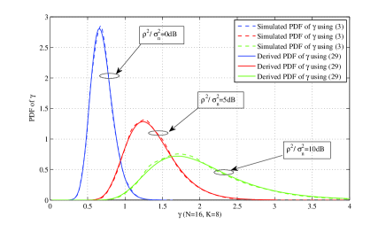
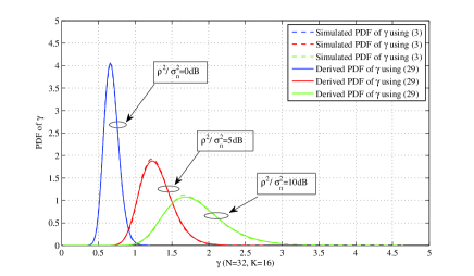
In order to evaluate the validity of the derived approximate PDF of SINR corresponding to the beamformer MF, by randomly generating many samples of 𝐑𝐀subscript𝐑𝐀\bf{h}_{k}, we calculate the exact values of SINR by using (2) and adopt the function ksdensity() in Matlab software to output the simulated PDF provided that parameters ρ𝜌\rho, N𝑁N, K𝐾K, Οƒh2subscriptsuperscript𝜎2β„Ž\sigma^{2}_{h}, and Οƒn2subscriptsuperscript𝜎2𝑛\sigma^{2}_{n} are fixed. The simulated exact PDF is used as a reference and compared with the derived approximate PDF of SINR directly computed by (29).
Refer to caption
Figure 1: PDF of SINR (N=16,K=8)formulae-sequence𝑁16𝐾8(N=16,K=8).
Refer to caption
Figure 2: PDF of SINR (N=32,K=16)formulae-sequence𝑁32𝐾16(N=32,K=16).
Refer to caption
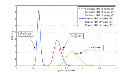
Figure 3: PDF of SINR (N=128,K=64)formulae-sequence𝑁128𝐾64(N=128,K=64).

Fig.Β 1, Fig.Β 2, and Fig.Β 3 demonstrates the curves of PDF of SINR for different typical SNRs defined as ρ2/Οƒn2superscript𝜌2subscriptsuperscript𝜎2𝑛\rho^{2}/\sigma^{2}_{n} for N=2​K𝑁2𝐾N=2K. Obviously, the derived PDFs are in very good agreement with the simulated PDFs for three different scenarios: N=16𝑁16N=16, N=32𝑁32N=32, and N=128𝑁128N=128.

Refer to caption
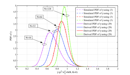
Figure 4: PDF of SINR (ρ2/Οƒn2=0​d​B,K=8)formulae-sequencesuperscript𝜌2subscriptsuperscript𝜎2𝑛0𝑑𝐡𝐾8(\rho^{2}/\sigma^{2}_{n}=0dB,K=8).
Refer to caption
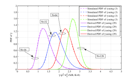
Figure 5: PDF of SINR (ρ2/Οƒn2=5​d​B,K=8)formulae-sequencesuperscript𝜌2subscriptsuperscript𝜎2𝑛5𝑑𝐡𝐾8(\rho^{2}/\sigma^{2}_{n}=5dB,K=8).
Refer to caption
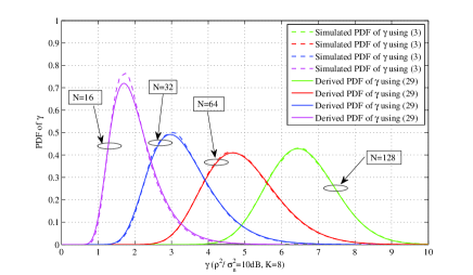
Figure 6: PDF of SINR (ρ2/Οƒn2=10​d​B,K=8)formulae-sequencesuperscript𝜌2subscriptsuperscript𝜎2𝑛10𝑑𝐡𝐾8(\rho^{2}/\sigma^{2}_{n}=10dB,K=8).

Fig.Β 4, Fig.Β 5, and Fig.Β 6 shows the curves of PDF of SINR for different typical values of N𝑁N for fixed K=8𝐾8K=8 and SNR. Obviously, the derived PDF matches well with the simulated PDF for three different scenarios: ρ2/Οƒn2=0​d​Bsuperscript𝜌2subscriptsuperscript𝜎2𝑛0𝑑𝐡\rho^{2}/\sigma^{2}_{n}=0dB, ρ2/Οƒn2=5​d​Bsuperscript𝜌2subscriptsuperscript𝜎2𝑛5𝑑𝐡\rho^{2}/\sigma^{2}_{n}=5dB and ρ2/Οƒn2=10​d​Bsuperscript𝜌2subscriptsuperscript𝜎2𝑛10𝑑𝐡\rho^{2}/\sigma^{2}_{n}=10dB.

From the above six figures, we also find, as N𝑁N increases, the simulated and derived PDFs of SINR converge to the same Gaussian distribution.

V Conclusion

We derived an approximate expression for the probability density function of SINR for medium-scale and large-scale MU-MIMO systems with MF beamformer. It is confirmed that the derived probability density function is very close to its counterpart obtained by simulation. The procedure of using the derived function to calculate the probability of symbol error is presented, which can also be applied to analyze the outage probability and average capacity.

References

  • [1] F. Rusek, D. Persson, Buon Kiong Lau, E.G. Larsson, T.L. Marzetta, O. Edfors, and F. Tufvesson, ”Scaling up MIMO: Opportunities and challenges with very large arrays,” IEEE Signal Process. Mag., vol. 30, no. 1, pp. 40-60, Jan. 2013.
  • [2] Thomas L. Marzetta, ”Noncooperative cellular wireless with unlimited numbers of base station antennas,” IEEE Trans. Wireless Commun., vol. 9, no. 11, pp. 3590-3600, Nov. 2010.
  • [3] Erik G. Larsson, Fredrik Tufvesson, Ove Edfors, and T.L. Marzetta, ”Massive MIMO for next generation wireless systems,” IEEE Commun. Mag., vol. 52, no. 2, pp. 186-195, Feb. 2014.
  • [4] Jacob Hoydis, Stephan ten Brink and M erouane Debbah, ”Massive MIMO in the UL/DL of cellular networks: How many antennas do we need,” IEEE J. Sel. Areas Commun., vol. 31, no. 2, pp. 160-171, Feb. 2013.
  • [5] Q. H. Spencer, A. L. Swindlehust, and M. Haardt, ”Zero-forcing methods for downlink spatial multiplexing in multiuser MIMO channels,” IEEE Trans. Signal Process., vol. 52, no. 2, pp. 461-471, Feb. 2004.
  • [6] Wiesel, Ami, Yonina C. Eldar, and Shlomo Shamai, ”Zero-forcing precoding and generalized inverses,” IEEE Trans. Signal Process., vol. 56, no. 9, pp. 4409-4418, Sept. 2008.
  • [7] Choi L U, and Murch R D, ”A transmit preprocessing technique for multiuser MIMO systems using a decomposition approach,” IEEE Trans. Wireless Commun., vol. 3, no. 1, pp. 20-24, Jan. 2004.
  • [8] M. Sadek, A. Tarighat, A. H. Sayed, ”A leakage-based precoding scheme for downlink mulit-user MIMO channels,” IEEE Trans. Wireless Commun., vol. 6, no. 5, pp. 1711-1721, May 2007.
  • [9] Liu W, Yang L L, and Hanzo L, ”SVD-assisted multiuser transmitter and multiuser detector design for MIMO systems,” IEEE Trans. Veh. Tech., vol. 58, no. 2, pp. 1016-1021, Feb. 2009.
  • [10] Peel C B, Hochwald B M, and Swindlehurst A L, ”A vector-perturbation technique for near-capacity multiantenna multiuser communication-part I: channel inversion and regularization,” IEEE Trans. Commun., vol. 53, no. 1, pp. 195-202, Jan. 2005.
  • [11] Hakjea S, Sang-Rim L, and Inkyu L, ”Generalized channel inversion methods for multiuser MIMO systems,” IEEE Trans. Commun., vol. 57, no. 11, pp. 3489-3499, Nov. 2009.
  • [12] Noh S, Zoltowski M, Sung Y, and D. J. Love, ”Pilot beam pattern design for channel estimation in massive MIMO systems,” IEEE J. Sel. Topics Signal Process., vol. 8, no. 5, pp. 787-801, Sept. 2014.
  • [13] Fernandes F, Ashikhmin A, Marzetta T L, ”Inter-cell Interference in Noncooperative TDD Large Scale Antenna Systems,” IEEE J. Sel. Areas Commun., vol. 31, no. 2, pp. 192-201, Feb. 2013.
  • [14] Chan-Sic Park, Yong-Suk Byun, Aman Miesso Bokiye, and D. J. Love, ”Complexity reduced zero-forcing beamforming in massive MIMO systems,” ITA’14, San Diego, CA, pp. 1-5, Feb. 2014.
  • [15] Kammoun A., Muller A., Bjornson, E., and Debbah M., ”Linear Precoding Based on Polynomial Expansion: Large-Scale Multi-Cell MIMO Systems,” IEEE J. Sel. Topics Signal Process., vol. 8, no. 5, pp. 861-875, Sep. 2014.
  • [16] A. Papoulis, S. U. Pillai, Probability, Random Variables and Stochastic Processes, 4th ed. New York, NY, USA: McGraw-Hill Higher Education, 2002.
  • [17] Andrea Goldsmith, Wireless Communications. Cambridge, England, UK: Cambridge University Press, 2005.