Modelling the Transfer Function for the Dark Energy Survey

Abstract

We present a forward-modelling simulation framework designed to model the data products from the Dark Energy Survey (DES). This forward-model process can be thought of as a transfer function — a mapping from cosmological/astronomical signals to the final data products used by the scientists. Using output from the cosmological simulations (the Blind Cosmology Challenge), we generate simulated images (the Ultra Fast Image Simulator, Bergé et al., 2013) and catalogs representative of the DES data. In this work we demonstrate the framework by simulating the 244 deg² coadd images and catalogs in 5 bands for the DES Science Verification (SV) data. The simulation output is compared with the corresponding data to show that major characteristics of the images and catalogs can be captured. We also point out several directions of future improvements. Two practical examples – star-galaxy classification and proximity effects on object detection – are then used to illustrate how one can use the simulations to address systematics issues in data analysis. With clear understanding of the simplifications in our model, we show that one can use the simulations side-by-side with data products to interpret the measurements. This forward modelling approach is generally applicable for other upcoming and future surveys. It provides a powerful tool for systematics studies which is sufficiently realistic and highly controllable.

1. Introduction

We have entered an exciting era of optical surveys. In recent years, the Kilo Degree Survey (KiDS, de Jong et al., 2013), the Panoramic Survey Telescope and Rapid Response System (Pan-STARRS, Hodapp et al., 2004), the Hyper Suprime-Cam Survey (HSC, Miyazaki et al., 2012), and the Dark Energy Survey (DES, The Dark Energy Survey Collaboration, 2005) have all started to take data. In particular, DES will cover the widest area (one eighth of the sky), and the resulting enormous datasets will allow one to achieve very high statistical precision in measuring cosmological parameters. We will soon be able to test with multiple cosmological probes, the standard $\Lambda$CDM cosmological model, and gain a better understanding of the nature of Dark Energy (Albrecht et al., 2006; Frieman et al., 2008; Huterer, 2010; Allen et al., 2011; Weinberg et al., 2013; Ruiz-Lapuente, 2014).

As the statistical uncertainties are reduced by orders of magnitude in these large datasets, various systematic uncertainties in analysing the data become important (Huterer et al., 2006; Amara & Réfrégier, 2008; Ho et al., 2013; Agarwal et al., 2014; Scolnic et al., 2014). Different cosmological probes are sensitive to different systematic effects. But generally, as all measurements begin from the same processed images and catalogs, the first-order systematic effects in these data products need to be well understood. In other words, one needs to understand how the information coming from the sky is transformed into the processed images and catalogs on which we base our scientific measurements. Moreover, one needs to understand how this transformation depends on the properties of the astronomical sources and the observing conditions. This paper seeks to understand this complicated process – the “transfer function” – for DES via forward-modelling. The goal of this work is to model the coadd images and the catalogs from DES. Although this framework still contains several simplifications (see $\S$3.1), it is the necessary first step in building a fully realistic simulation pipeline. Note also that although we focus on DES in this paper, our methodology is generally applicable for all upcoming and future large surveys.

Figure 1.— Footprint for the DES SV data used in this work. The different colours indicate the different types of fields: the blue and green areas are the SPT wide-field coverage, the grey areas indicate the pointed cluster fields outside of the SPT fields, and the red areas indicate the Supernova fields.

The concept of modelling the transfer function for a specific experiment has a long history in the field of particle physics (Bengtsson & Sjöstrand, 1987; Nelson & Namito, 1990; Marchesini et al., 1992; Agostinelli et al., 2003; Binder & Heermann, 2010; Beringer et al., 2012). In fact, the results of particle physics experiments can only be interpreted in terms of their corresponding Monte Carlo simulations. In optical astronomy, however, the idea of forward-modelling is less mature, despite the fact that highly developed simulation tools exist for individual steps of the transfer function. For example, cosmological simulations such as Hilbert et al. (2009); Kiessling et al. (2011); Gerke et al. (2013); Riebe et al. (2013); White et al. (2013) begin with N-body simulations and develop prescriptions for assigning astronomical objects to dark matter halos. Springel & Hernquist (2003); Smith et al. (2008) and Vogelsberger et al. (2012) use different techniques to simulate various hydrodynamic processes in structure formation and link to observables related to cosmology. Peng et al. (2002) uses simulated galaxy images to help understand the study of galaxy morphology. Bertin (2009); Bridle et al. (2010); Kitching et al. (2012); Bergé et al. (2013) simulate astronomical images with simple instrumental effects to understand how well one can recover information from noisy data. Finally, Peterson & Jernigan (2013) focuses on the detail modelling of the astronomical instrument to understand how the instrument design affects the imaging data. Although these different simulations are very helpful for understanding the technical issues in the separate areas, one cannot straightforwardly infer how the results in different parts of the transfer function couple to each other. The recent attempt described in Connolly et al. (2010) is one of the first efforts to consolidate the issue by connecting all types to an end-to-end simulation framework for one specific project, the Large Synoptics Survey Telescope (LSST). Our work is based on the same philosophy, but instead of modelling a future instrument like LSST, the aim is to model DES, which is currently taking data.

We extend from the Blind Cosmology Challenge simulations (BCC, Busha et al., 2013) to include processed images from the Ultra Fast Image Generator (UFig, Bergé et al., 2013) and catalog products which come from a similar analysis pipeline as that used in the DES Data Management (DESDM, Ngeow et al., 2006; Sevilla et al., 2011; Desai et al., 2012; Mohr et al., 2012). Our implementation is similar to the earlier DES data challenges described in Lin et al. (2010) and Sevilla et al. (2011), where DES simulations were generated before the existence of data to test data management and science analysis software. This work is complementary to the earlier data challenges in that the simulations in this work is guided by the actual DES data and data processing pipeline being used, which was not available at the time of the data challenge.

This paper is organised as follows: In $\S$2, we briefly introduce the Dark Energy Survey and the relevant data products that are used in this paper. In $\S$3 we describe in detail the forward-modelling framework, including individual simulation and analysis tools, as well as the interfacing between them. A series of quality assurance tests are performed in $\S$4 to examine the output products of our framework. We cross-check with early DES data to ensure the output captures the main characteristics of the data. We then demonstrate in $\S$5 two practical applications where we use this forward-modelling framework to address specific technical questions in the data analysis process. Finally, we conclude in $\S$6.

An example of the simulation output and supporting documentation from this work can be found at http://www.phys.ethz.ch/~ast/cosmo/bcc_ufig_public/.

2. The Dark Energy Survey

The Dark Energy Survey (DES) is a wide-field optical survey that officially began in August 2013 (Diehl et al., 2014) and will continue to survey the sky through 2018. The full DES footprint will cover one eighth of the full sky (5,000 deg²) in five optical bands ($grizY$). The homogeneous wide-field nature of the dataset will be important for cosmology studies on very large scales. The primary instrument for DES is a newly assembled wide-field (3 deg²) mosaic camera, the Dark Energy Camera (DECam, Diehl & Dark Energy Survey Collaboration, 2012), installed on the 4m Blanco telescope at the Cerro Tololo Inter-American Observatory (CTIO) in Chile.

The raw images taken each night are collected and jointly processed with the DESDM software. In addition to the zeroth-order image processing (flat-fielding, bias correction, de-trending etc.), the DESDM pipeline contains mainly software packages described in Ngeow et al. (2006); Sevilla et al. (2011); Desai et al. (2012); Mohr et al. (2012) – SCAMP (astrometry, Bertin, 2006), SWARP (image coaddition, Bertin et al., 2002), PSFEx (modelling of the point-spread-function, Bertin, 2011) and SExtractor (object detection and measurement, Bertin & Arnouts, 1996). With continual improvement in the pipeline, DESDM performs regular releases of the data products. The main product from DESDM are images and catalogs of objects with calibrated properties.

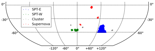
The initial pre-season of DES observations were labeled as Science Verification (SV) imaging, which took place from November 2012 – February 2013. These images were processed by the DESDM pipeline version “SVA1” (Yanny et al., in prep) to produce coadd images and SExtractor catalogs. Additional quality checks and calibration were performed by DES scientists, which included cropping out bad regions contaminated by satellite and airplane trails, as well as the region at declination $<-61^{\circ}$ which has a very high stellar density due to the presence of the Large Megallanic Cloud (SVA1 Gold; Rykoff et al., in prep). After all cuts, the total sky coverage is 244 $\mathrm{deg}^{2}$ of $griz$ imaging. This includes several selected wide fields, pointed cluster fields (RXC J2248.7-4431, 1E 0657-56, SCSO J233227-535827, and El Gordo), and deep supernova (SN) fields. Figure 1 shows the full SVA1 footprint and how the different fields are distributed. The SN fields are revisited every 5-7 days with longer exposures, and are therefore 1-2 magnitudes deeper than the other fields, particularly in the $i$ and $z$ bands. In this work, we base our forward-modelling framework on the SVA1 Gold catalogs. As the DESDM software and image quality continue to improve for future releases, our modelling framework will adjust accordingly.

3. Forward-modelling

In this section we briefly introduce the three major elements of our forward-modelling framework: two simulation tools ($\S$3.2, $\S$3.3) and the analysis software ($\S$3.4). We then describe how the interfaces between the three components are implemented ($\S$3.5) and the computational cost ($\S$3.6). First, however, we list in $\S$3.1 the main simplifications used in this framework.

3.1. Simplifications

The current framework as described below contains several simplifications. As we will discuss in $\S$6, more sophistication and realism is planned to be added to the framework as required from different science cases. The main simplifications of the current framework are the following: (1) We begin the forward-modelling from coadd images instead of single-exposure images, thus bypass the process of stacking images. (2) The PSF, airmass, background (limiting magnitude), quantum efficiency, and throughput are constant in each filter with no spatial variation across an image. (3) The background model is simplistic (Gaussian noise plus Lanczos resampling) and does not properly model the correlation of noise in the images. (4) There are no artefacts such as bad/hot columns on the detectors, satellites, cosmic rays, etc..

It is important to stress that the focus of this forward-modelling framework is not to make simulations that are identical to the data (nor is it possible to do so exactly). Rather, it is to capture the important characteristics of the data in a controlled environment where we know the truth. This allows us to interpret the measurements in a clean fashion within the limitations of the simulations. As a result, despite these simplifications, many data-related issues can already be investigated as we demonstrate in $\S$4 and $\S$5. The results from these simplified simulations would also be important for interpreting more realistic simulations in the future as we incorporate more physics in the forward model.

3.2. The mock sky catalog

The primary input to our framework is a mock sky catalogs of astronomical sources. In this work, we use the Aadvark v1.0d catalogs generated as part of the BCC. The BCC catalog generation begins with particle light cones from a series of large (1-4 Gpc/h) N-body simulations with a defined cosmology (a flat LCDM cosmology in this case). The Adding Density Determined GAlaxies to Lightcone Simulations algorithm (ADDGALS, Busha et al., 2013) associates galaxies to the dark matter particles by using a Sub-Halo Abundance Matching (SHAM) catalog (Conroy et al., 2006; Behroozi et al., 2010) generated from a high resolution, low-volume tuning simulation to determine a probabilistic relation between a galaxy’s magnitude and its local dark matter density. The algorithm then assigns basic properties (luminosity, colour, etc.) to each galaxy using a training set of spectroscopic data from the SDSS DR6 Value-Added Galaxy Catalog (Blanton et al., 2005) to match simulated galaxies to observed counterparts using the local galaxy environment. The training procedure is performed at low redshift and extrapolated to high redshift so that the colour distribution simultaneously matches the photometric data in SDSS DR8 and DEEP2. The intrinsic shape and size of each galaxy is then set to match to observations from the SuprimeCam deep $i^{\prime}$-band data (Dietrich et al., 2012). Finally, the galaxies are lensed by the multiple-plane ray-tracing code, Curved-sky grAvitational Lensing for Cosmological Light conE simulatioNS (CALCLENS, Becker, 2013) to give perturbed shapes, positions and magnitudes. Additionally, a stellar distribution is added based on the TRIdimentional modeL of thE GALaxy code (Trilegal, Girardi et al., 2012; Balbinot et al., 2012), and the quasar model is based on Maddox et al. (2012). The full details of the BCC catalogs would be described in an upcoming paper.

These BCC catalogs serve as the “true” sky after the sources have been lensed by the large scale structures before the light enters the atmosphere. For this work, the main properties used in the BCC catalogs are the magnitude, size, colour, redshift and shape distributions of objects. The main requirement is that these distributions in the BCC catalog are modelled for objects fainter than the limiting magnitude of the dataset we wish to model.

There are several advantages of using such sophisticated cosmological simulations as our input compared to using parametrised star/galaxy distributions [cf. our earlier work in Bergé et al. (2013)]. First, one preserves the cosmological clustering of the galaxies. Second, one simultaneously retains a self-consistent cosmology between clustering, lensing, and redshift evolution of galaxies. Finally, the correlation between the magnitudes of objects in different filter bands (i.e. colours) are also self-consistent. Note however, that the BCC catalogs cut off at a magnitude only slightly deeper than the DES main survey limiting magnitude. This suggests that the fainter objects that contribute to the background will be missing in our images and we cannot simulate properly the deeper Supernova fields. One would need to examine the impact of these missing faint objects on the measurement of interest when using the simulations from this framework.

3.3. The image simulation software

The Ultra Fast Image Generator (UFig, for full detail of the implementation of UFig, see, Bergé et al., 2013) is a fast image simulation code that generates scientific astronomical images that capture the major characteristics of a given instrument, as specified by the user. The computational time required for UFig to generate images in this work is much shorter than the time required to analyse the images (see $\S$3.6).

We briefly describe here the image rendering process in UFig. First, the apparent magnitudes of stars and galaxies are converted into number of photons expected at the focal plane, given the atmosphere and instrumental throughput in the specific filter band. Then, images of the galaxies are generated by drawing probabilistically, one photon at a time, from the galaxy profile model (single Sérsic profile with varying Sérsic index, Sérsic, 1963). Next, we construct a model for the point spread function (PSF) given a desired seeing value. The galaxies are then convolved with the PSF model by displacing the photons randomly according to a probability density function described by the PSF profile. The image is then pixelated. Stars are generated directly on the pixels, with the same profile as the PSF model and appropriate Poisson noise on the pixel values. The stars and galaxies are generated via different approaches to optimise the computational speed. These pixel values are then converted into electronic units (ADUs) and an user-specified Gaussian noise is added. Finally, the full image is convolved with a Lanczos filter of size 3 (Duchon, 1979) to simulate the correlation of the noise in a coadd image. The full image is then rescaled to a given magnitude zeropoint.

3.4. The data processing software

As mentioned in $\S$2, the DESDM pipeline uses a suite of software packages to produce the final catalog. Since we simulate the processed coadd images directly from UFig ($\S$3.3), we bypass several steps in the DESDM pipeline. These are simplifications that can be improved upon in the future. The two main packages involved in our framework are PSFEx and SExtractor.

PSFEx is a software that constructs a model for the PSF of an image. Accurately knowing the PSF is important for later steps in the pipeline such as photometry measurements and galaxy profile-fitting. SExtractor is the main measurement software in the process. It estimates the background, detects objects, and conducts the basic measurements for each object. These include magnitudes estimated with several different approaches, various size estimates, parametrised model of the object profile, and classifiers that help the user identify different types of objects. As the output is sensitive to detailed settings in the PSFEx and SExtractor configuration, we match the setting to that used in the SVA1 catalog whenever possible.

3.5. Bridging heaven and earth

The three basic elements of the forward-modelling framework described above are interfaced and connected as described in the following steps.

Figure 2.— A 500$\times$500 pixel region of an arbitrary $i$-band DES image (left) and its simulation counterpart (right). The scales in both images are the same. Note that the objects are not matched one-to-one in these images, but the statistical clustering and object properties appear qualitatively similar. Note also that the texture of the background is slightly different in the simulations compared to the data, indicating that improvements are needed for the background model.

3.5.1 BCC catalog $\rightarrow$ UFig catalog

The first step involves converting the “sky information” in the BCC catalogs into “image information” that can be used by UFig. We start by defining pointing positions on the sky, from which we draw a 0.75$\times$0.75 deg² area where the image will be simulated. The image size is defined by that of DESDM coadd images.

The information in the BCC catalogs is then translated into UFig internal parameters. Object coordinates are converted into physical positions on the image with the appropriate World Coordinate System (WCS) transformation. All images are linearly projected from the sky with a pixel scale of 0.27 arcsec/pixel. The apparent magnitude of stars and galaxies, as well as the ellipticity of galaxies are taken directly from the BCC catalogs. The intrinsic galaxy size information is based on the BCC catalogs but adjusted slightly so that the 2d distribution in apparent magnitude and intrinsic size is consistent with that derived from the COSMOS data (Jouvel et al., 2009). The adjustment is needed because the BCC catalog takes an approximate approach when converting the observed galaxy size into the intrinsic galaxy size. Finally, the galaxy is modelled by a single Sérsic profile, where the Sérsic indicies are band-independent and drawn randomly from the following distributions:

$$f(n)=0.2\\ +\left\{\begin{array}[]{ll}\exp(N(0.3,0.5)+N(1.6,0.4))&\mbox{if $i<20$};\\ \exp(N(0.2,1))&\mbox{if $i\geq 20$},\end{array}\right.$$ (1)

$N(\mu,\sigma)$ denotes a normal distribution of mean $\mu$ and standard deviation $\sigma$. Equation 1 was derived in Bergé et al. (2013) from fitting deep $i$-band images (Griffith et al., 2012). A more sophisticated Sérsic distribution that also takes into account the band dependencies would be a direction of future improvement. The Sérsic index is the only parameter of the source properties external to the BCC catalogs.

3.5.2 UFig catalog $\rightarrow$ UFig image

Next, we simulate a UFig image from the source catalog generated from the previous step. The instrument characteristics and observing conditions need to be specified for each image. These parameters include the throughput, the Charge-Coupled Device (CCD) characteristics, the seeing condition and the sky brightness.

In all the simulations in this paper, we take the major instrumental parameters from the official DES Exposure Time Calculator (ETC) as listed in Table 1. The atmospheric throughput describes the fraction of light that passes through the atmosphere at zenith. The telescope throughput describes the fraction of light that passes through the telescope and arrives at the focal plane. The mean wavelength and the bandwidth specify the basic properties of the filters. The quantum efficiency measures the fraction of photons that is converted into digital signal in the CCD. All quantities in this table are average values. Note also that we follow the DESDM convention and normalise the coadd images to either 90 ($griz$-band) or 45 ($Y$-band) seconds-equivalent exposures.

On the other hand, the image-specific parameters (eg. exposure time, seeing, background noise) are tuned to the specific data we wish to model. We use a circular Moffat PSF model with $\beta=3.5$ (Moffat, 1969), which is is typically a good description for ground-based optical PSFs. The PSF is assumed to be spatially constant in each image and have a FWHM (which can be specified for a Moffat profile with given $\beta$ parameter) equal to the mean seeing in the data of interest. Similarly, the background level is set so that the expected limiting magnitude agrees with the data (see Appendix A for details on the derivation of the background noise).

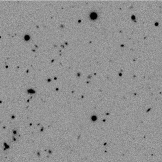
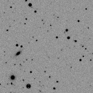
Figure 2 shows one arbitrary DES image in $i$-band and its simulation counterpart. Note that the objects in the images are not matched one-to-one, but the statistical clustering and noise properties appear qualitatively similar from visual inspection. We also note that due to the simplification in the background model (Gaussian noise plus Lanczos resampling), the texture of the background appears to be qualitatively different from the data.

Table 1Basic instrumental parameters for the UFig image simulations.

Filter	$g$	$r$	$i$	$z$	$Y$
Atmosphere throughput	0.8	0.9	0.9	0.9	0.95
Telescope throughput	0.43	0.51	0.56	0.56	0.19
Mean wavelength (nm)	473	638	775	922	995
Bandwidth (nm)	147	141	147	147	50
Quantum efficiency	0.7	0.75	0.85	0.8	0.3

3.5.3 UFig image $\rightarrow$ DESDM catalog

In this step we run the DESDM software on the UFig images to produce SExtractor catalogs. First, the PSF model is estimated by PSFEx on each of the single-band coadd images. Then we follow the procedure implemented in DESDM and make a deep “detection image” by stacking the coadd images in three bands ($riz$). Objects are detected on the “detection image” but the properties of each object are measured on the single-band images using SExtractor. The software versions used in this work are: SExtractor v2.18.10, PSFEx v3.17.0 and SWARP v2.36.2. The configuration files for SExtractor and PSFEx can be found at: http://www.phys.ethz.ch/~ast/cosmo/bcc_ufig_public/bcc_ufig_config.tar.gz

This is the most time-consuming step in the framework, as SExtractor carries out a large number of measurements and galaxy profile-fitting operations. However, depending on the specific science interest, it is possible to eliminate some of the SExtractor functionalities and make this step faster. For instance, eliminating the process of fitting galaxy profiles speeds up the procedure by a factor of $\sim 100$.

Figure 3.— Distribution of the differences in three magnitude measurements and the true input magnitude as a function of the input magnitude. From top to bottom are the SExtractor magnitudes MAG_AUTO, MAG_MODEL and MAG_DETMODEL. Left and right panels are for stars and galaxies respectively. All plots are generated for one arbitrary $i$-band image in our simulation. Note that the colour scales are logarithmic.

3.5.4 DESDM catalog $\rightarrow$ BCC catalog

Finally, to close the loop, the catalogs generated from SExtractor above are matched to the input BCC catalogs by the position on the sky, and a matching file containing the galaxy ID’s in the input and output catalog is written out. The matching process is sped up by first dividing each image into 20 smaller areas, and then matching within the subareas. It is this matching that gives us a model of the transfer function for DES data. We now have a mapping between the input signal from the sky and the final catalogs one uses for science.

Figure 4.— Distribution of of three magnitude measurements and the associated errors as quoted from the SExtractor output. From left to right are the SExtractor magnitudes MAG_AUTO, MAG_APER_4 (2 arcsec) and MAG_MODEL. The top row shows that measured from one arbitrary $i$-band SV image and the bottom shows the measurement from the corresponding simulated image. The colour scales are logarithmic. Note that the middle bottom panel shows that most of the data points lie on a very tight line in this parameter space.

3.6. Data volume and computational cost

The images and catalogs in this work are generated on the Brutus cluster at ETH Zurich. The typical run time to generate the FITS image and SExtractor catalog for a 0.75$\times$0.75 deg² patch of sky in one filter band for our SVA1 simulation set (see $\S$4) is summarised in Table 2, together with the file sizes. The runtimes is calculated for running with one core on AMD Opteron 6174/8380/8384 machines. Generally, the run time of the image generation scales with the number of photons, or exposure time and the run time for the analysis processes scale with the number of objects detected. The run time is dominated by the Source Extractor analysis process.

Note that Table 2 does not include the generation of the BCC catalogs upstream to this work, which includes the N-body simulations and the input galaxy/star/quasar catalogs. To estimate the computational cost for the full end-to-end framework, one would also need to take into account these factors, which adds a total of $\sim 340$k CPU hours to the computational time.

Table 2Summary for the average runtime on one core and size of output files for the SVA1 simulations in this work. All numbers are quoted for one coadd image in one filter, and all data size are quoted after gzip compression.

Output	Run time	Format	Size
Coadd image	7.0 min	FITS	356 M
SExtractor catalog	2.5 hr	FITS	53 M
Matching file	3.8 min	ASCII	1.4 M

4. Quality Assurance: forward-modelling the DES SVA1 data

In this section we present several basic quality assurance tests on the output catalog of the above simulation framework. The main goal is to show that our framework produces reliable catalogs that can be used for interpreting scientific data under well understood assumptions. For regimes where the simulations do not properly model the data, we identify areas for improvement in our model.

We set our target to model the DES SVA1 dataset described in $\S$2. We generate coadd images and catalogs covering the SVA1 footprint (Figure 1) in all 5 filter bands. In addition to the basic parameters listed in Table 1, we also use compiled maps for mean observational parameters from the data themselves (seeing, limiting magnitude, magnitude zeropoint). These maps are generated similar to the systematics maps described in Leistedt et al. (2013). For each of our images in each filter band, we find the corresponding region of sky in the maps. Then, we take the median value of the maps to be the observational parameters for this image. Note that for modelling another dataset, even with the same instrument, the results could differ significantly. A portion of the SVA1 simulation output and supporting documentation can be found at http://www.phys.ethz.ch/~ast/cosmo/bcc_ufig_public/. The total number of coadd images is 480 in $griz$-bands and 432 in $Y$-band.

Below we focus on examining three basic measurements of the detected objects in the images – magnitude, size and object number counts.

4.1. Magnitude

Photometry lies at the centre of many science analyses. Yet, in typical astronomical data, magnitude measurements and the corresponding errors are often hard to predict from first principles due to the noisiness of the data, the non-linear nature of the measurement procedure, and the coupling to the objects’ size and profile. We examine here the relation between the input and different measured magnitudes. Then we compare the general behaviour of the different magnitude measurements in the SVA1 data compared with that in our simulations. Similar analyses have been done in Sevilla et al. (2011); Rossetto et al. (2011) for early DES simulations.

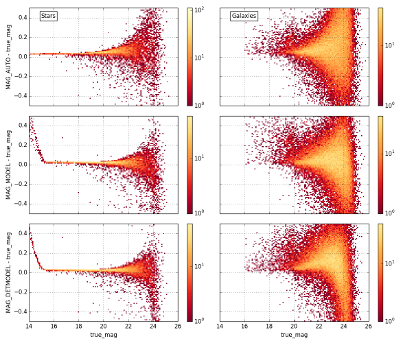
In Figure 3 we show the distribution of the difference between measured and input magnitude as a function of input magnitude for three different magnitude estimates from SExtractor (MAG_AUTO, MAG_MODEL and MAG_DETMODEL) on one arbitrarily selected $i$-band image. MAG_AUTO is measured by summing the flux in an ellipse scaled to the Kron radius (Kron, 1980); MAG_MODEL is measured by fitting the object with a given model and estimating the flux for this model; MAG_DETMODEL is similar to MAG_MODEL but first carries out the model fitting on the detection image, and then fits the overall normalisation of this model to each single-band image separately. MAG_DETMODEL thus has a consistent galaxy model for the same galaxy across all filters, which is primarily useful for colour measurements. For SVA1, MAG_MODEL and MAG_DETMODEL use a single exponential profile for the galaxy model.

The general trend between all three estimates is that the measured magnitudes tend to be biased high and that faint objects have larger photometric errors than bright objects. The bias is due to the fact that the magnitudes are all calculated within some finite pixels defined by the signal-to-noise of each pixel, whereas in reality, light can fall much further out. For the stars, the bias is at the 0.01–0.02 level at the bright end, with MAG_AUTO slightly higher than the other two. This is sensible as the fitting methods (MAG_MODEL and MAG_DETMODEL) does account for some of the low-level wings. Model fitting also results in smaller scatter at the faint end and the sharp turnoff at the very bright end, where the model fails to fit bright star profiles. For galaxies, there is a small “bump” feature at magnitude $\sim 20$. The feature is a result of the input galaxy model, where galaxies have different distribution of profiles above and below $i=20$ (Equation 1). The galaxy MAG_AUTO measurements behave similar to that for the stars with slightly more scatter. MAG_MODEL and MAG_DETMODEL, however, does not improve significantly the magnitude measurements compared to MAG_AUTO. This could indicate that the model for the galaxy profiles used by MAG_MODEL and MAG_DETMODEL is insufficient for the wide range of galaxy profiles in the simulations (and in data). We also see that MAG_MODEL is less biased compared to MAG_DETMODEL. This is because MAG_DETMODEL derives the galaxy model from the detection image ($riz$-coadd) instead of the image where the magnitude is measured. Note that, the difference would be larger in real data, where unlike in our simulations, the galaxy and the PSF profiles change in different filter bands.

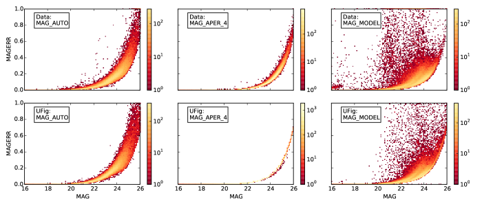
In Figure 4 we show the magnitude error against magnitude for one arbitrary $i$-band DES image and the corresponding UFig simulation. We examine the behaviour of three different magnitude estimates in the SExtractor catalog. All objects in both catalogs are plotted. The broad features in the different panels agree between the simulation and the data with some discrepancies that are expected from the simplifications and assumptions described in $\S$3. First, in the MAGERR_AUTO - MAG_AUTO panel agree down to $i\sim 24.5$, but there are more objects in the simulations compared to the data at $i>24.5$. This shows that the simulation is able to reproduce the behaviour of the magnitude error at $i<24.5$, which is sufficiently deep for DES. For the fainter objects, one should take caution when interpreting results from the simulations in this regime. Second, the MAGERR_APER_4 - MAG_APER_4 relation in the simulation lies on top of that from data. This confirms that our noise model behaves as expected (see $\S$A). The data contains more scatter compared to the simulations. This is expected as the limiting magnitude varies within an image in data, while we have assumed it to be constant in our simulations. Finally, for the MAG_MODEL - MAGERR_MODEL panel, both data and simulation show an overall more complicated shape of the distribution. The same qualitative feature can be seen in both plots, such as the sharp drop of numbers at MAGERR_MODEL$\sim 0.2$, the faint could of objects with large MAGERR_MODEL at MAG_MODEL$\sim 24$. These indicate that our model of the intrinsic galaxy morphology (size and Sérsic index) is reasonable. The details in the two distributions are however difference. This is an indication that improvements are needed in the future in this area, and one should take caution when using MAG_MODEL in our simulations.

Figure 5.— Distribution of the difference in measured size and input size r50 as a function of r50 (left), Sérsic index (middle) and magnitude (right). r50 is defined in Equation 2. All plots are generated for one arbitrary $i$-band image in our simulation. And more that the colour scales are logarithmic.

Figure 6.— Measured size distribution for all objects from the UFig simulations (black) compared to the SVA1 data (red) in the same area. The grey lines show the same distribution as the black line, but for other tiles in our SVA1 simulation that have limiting magnitudes and seeing conditions within 1% of the region of interest. The disagreement in the distributions is consistent with the variation from cosmic variance.

4.2. Size

The first-order morphological information we can measure from an object’s image is its observed size. The measured size of an object in a noisy image is usually defined in terms of the flux in a set of pixels that are assigned to this object – for example, the parameter FLUX_RADIUS  in SExtractor refers to the radius within which 50% of the total flux is enclosed. The measured size is thus coupled with magnitude measurements and is sensitive to the noise in the image, the PSF and the intrinsic object profile.

In Figure 5, we show the distribution of the difference between measured object size and input size (r50) as a function of input size, Sérsic index and true magnitude for all detected objects in one arbitrary $i$-band image. The “input size” r50 here refers to the expected half-light radius of the object after convolving with the PSF. We calculate it via the following empirical relation:

$$\rm{r50}=\sqrt{\rm{r50_{in}}^{2}+\rm{r_{PSF}}^{2}/2.355},$$ (2)

where $\rm{r50_{in}}$ is the intrinsic half-light radius given by the BCC catalog and $\rm{r_{PSF}}$ is the seeing for that image. The numerical factor 2.355 is derived empirically to account for the change of the apparent galaxy size when convolved with the PSF. Note that Equation 2 is only an approximate relation between $\rm{r50_{in}}$ and $\rm{r50}$. Nevertheless, we use it here to illustrate the qualitative behaviour of the size measurements in our catalogs.

Figure 5 shows that small, faint, disk-like galaxies have larger errors on the size measurement. The distribution of the errors are asymmetric with more objects biased small. The origin of the asymmetry comes from the fact that SExtractor measures the sizes with a finite set of pixels while the galaxy profile generally extends beyond that.

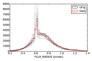
In Figure 6 we compare the measured size distribution of all the detected objects in one arbitrary $i$-band image in the SVA1 data and the corresponding simulation. Also overlaid in grey are 10 other size distributions from the simulations that have limiting magnitude and seeing values within 1% of this image, these curves give an estimate of the variation in the size distribution due to cosmic variance. We find that the measured size distribution in our simulations are consistent with that measured in data within cosmic variance. The narrow peak at FLUX_RADIUS$\sim 0.6$ arcsec corresponds to the seeing value for this image. The peak is broadened in the data since unlike in the simulations, there exists seeing variation within each image. The size distribution of the remaining objects (mostly galaxies) match very well between the data and simulations, especially on the high and low end where it is less sensitive to our assumption of constant seeing. Seeing variation is thus one important factor to improve in future developments.

4.3. Number density

Figure 7.— Galaxy (black) and star (red) number densities as a function of the limiting (2 arcsec) aperture magnitude (left), seeing (middle) and galactic latitude (right). These numbers are calculated from all objects detected in all the $i$-band images in the SVA1 simulations in this work. Each data point represents one image in our simulation. The discontinuous distribution of data points in the x-axis of the right panel reflects the SVA1 footprint.

Table 3Object number density (per sq. arcmin) from data and our simulations under different magnitude (MAG_AUTO) cuts.

	Data	Simulation
All objects	27.79	31.05
$15<i<19$	1.06	1.01
$15<i<21$	3.43	3.85
$15<i<23$	11.95	12.82

Finally, we examine the detected star and galaxy number densities. This is important because it simultaneously checks the input source distribution, the image simulation and the analysis software.

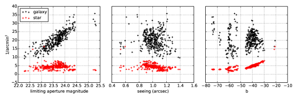
In Figure 7 we show the star and galaxy number density in all the $i$-band simulated SVA1 images as a function of limiting magnitude, seeing and galactic latitude. We observe that the general behaviour of the number counts follows expectation. In deeper fields the number density of stars and galaxies both increase. The group of data points on the far right are the Supernova fields (see Figure 1) where the total exposure time is significantly longer than in the rest of the fields. Note however, the input BCC catalogs are not necessarily complete at those magnitudes, thus one should be careful in interpreting the results there and only treat those data points as lower bounds. The dependence on seeing is also expected (keeping in mind that seeing and limiting magnitude are not independent) – higher seeing gives slightly lower number density since the signal-to-noise of the objects decreases going to higher seeing. Finally, we look at the correlation between number density and the galactic latitude as a check for the input source catalog. We find that the stellar density, as expected, increases towards the galactic plane, whereas the galaxies do not. The discontinuous distribution of data points in the x-axis reflects the SVA1 footprint.

To compare the number counts derived from simulations and data, we calculate the mean source density as a function of magnitude cuts for both the SVA1 catalog and our simulations. We use all objects in the catalogs and do not make distinction between stars and galaxies. We choose to do so to avoid making choices in the object selection. This also means that we are accounting for spurious detections from noise, blended objects and artefacts. Table 3 summarises our results. We find that the data and the simulations agree at the $\sim$10% level. The agreement is best at the bright end, where the errors in the object property as well as the noise is more accurate. The agreement is not perfect, but rather encouraging, given the current uncertainty in the source catalog, the galaxy profile model and the noise model.

5. Applications

In this section we describe two example cases where we use the simulation products described in $\S$4 to help answer questions in the data analysis process. The advantage of using this framework is that the simulations are sufficiently realistic, yet, we have full control over every stage of the simulation and data processing pipeline. For use of our simulations in scientific analyses on the DES SV data, see Rykoff et al. (in prep.).

Figure 8.— Efficiency (E) and purity (P) for the star and galaxy sample of three star-galaxy classifiers for one arbitrary $i$-band images in our SVA1 simulations. The three classifiers are described in Table 4.

Table 4Cuts used in the three classifiers: CLASS_STAR, SPREAD_MODEL and MODEST_CLASS. All of these cuts have an additional cut on FLAGS$<=$3 and 5 sigma detection. For full description of MODEST_CLASS see footnote below.

Galaxies	Stars
CLASS_STAR$<$0.95	CLASS_STAR$>$0.95
SPREAD_MODEL$>0.002$	SPREAD_MODEL$<0.002$
MODEST_CLASS =1a	MODEST_CLASS=2b

Figure 9.— Median efficiency (E) and purity (P) for galaxy classification of all simulated SVA1 images at $18.5<$MAG_AUTO$<19.5$ (left) and $22.5<$MAG_AUTO$<23.5$ (right), as a function of seeing of that image. The three classifiers are described in Table 4. Note that the y-axis has very different scales.

5.1. Star-galaxy classification

Identifying stars and galaxies in optical images is one of the most basic operations in the data analysis pipeline. Depending on the science application, one would demand good efficiency and/or purity in the star sample and/or the galaxy sample. For example, in weak gravitational lensing, one would require a pure star sample for the PSF estimation, and a pure galaxy sample for un-contaminated lensing signal. On the other hand, for study of galaxy evolution, the completeness of the galaxy sample is also important in order for one to extract global behaviours of the galaxy population. We define the star/galaxy classification efficiency ($E$) and purity ($P$) below:

$$E({\rm X})=\frac{{\rm\#\;of\;objects\;correctly\;identified\;as\;X}}{{\rm\#\;of\;all\;X}}$$ (3)

$$P({\rm X})=\frac{{\rm\#\;of\;objects\;correctly\;identified\;as\;X}}{{\rm\#\;of\;objects\;identified\;as\;X}}$$ (4)

where X is either stars or galaxies.

The problem is challenging, however, in typical ground-based imaging data. With typical seeing and noise conditions in these images, small, faint galaxies become indistinguishable from stars. A wide range of techniques have been developed to resolve this problem (Henrion et al., 2011; Fadely et al., 2012; Soumagnac et al., 2013). Standard star-galaxy classifiers use morphological information of the stars, more advanced ones incorporate also the colour information (Pollo et al., 2010). The simulations from this work, with both realistic image characteristics and colour information, offer a generic tool for different methods to be tested on before applying to data. Moreover, since the simulations are tailored for a specific set of data, one can consistently evaluate the effect of star-galaxy separation on specific science measurements performed on the same dataset.

Figure 10.— Degradation of detection efficiency due to proximity effects around bright objects evaluated for one arbitrary $i$-band image in our SVA1 simulation. In the left panel, the four curves indicate the detection efficiency for source galaxies in the magnitude range $18<i<24$ around center galaxies in different magnitude bins. The x-axis shows the distance from the center galaxy. The y-axis shows the fraction of source galaxies detected. All curves are normalized so that the level measured at 20 arcsec is 1. This removes the detection efficiency from the finite depth. The right panel shows only the magnitude bin $19<i<20$ in the left panel, but overlays in grey results for 10 other random images. The grey lines agree with the green line within error bars, despite the different observational conditions. Also plotted in black is the result when we replace the centre galaxies with stars, which results in a qualitatively different shape of curve.

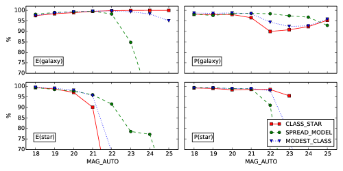
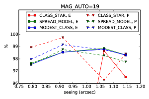
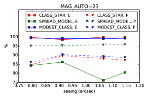
Here, we show an example of quantifying the performance of three single-band cut-based star-galaxy classifiers which are based solely on the SExtractor catalogs. The three classifiers which we label as CLASS_STAR, SPREAD_MODEL, and MODEST_CLASS are described in Table 4. CLASS_STAR is a pre-trained Artificial Neural Network method that uses several of the photometric and shape information in the SExtractor catalogs. It works well at the bright end but is limited by requiring the user to know the approximate seeing of the image prior to processing. SPREAD_MODEL (Mohr et al., 2012; Bouy et al., 2013) uses pixel-level morphological information and compares the profile of each object with the local PSF. For faint objects, where the classification is most challenging, CLASS_STAR with the current settings tends to classify all objects as galaxies at the faint end while a naive SPREAD_MODEL classifier with constant threshold tends to classify all objects as stars. MODEST_CLASS is a new classifier used for SVA1 Gold that has been developed empirically and tested on DES imaging of COSMOS fields with Hubble Space Telescope ACS imaging. It is primarily based on SPREAD_MODEL, and attempts to fix the faint galaxy classification by including the error on SPREAD_MODEL.

We evaluate the $\rm E$ and $\rm P$ statistics for stars and galaxies on one arbitrary $i$-band image in our SVA1 simulations as a function of the measured MAG_AUTO. The results are shown in Figure 8. In this particular image, the simulations confirm nicely what we expect from the construction of the three classifiers (see above). For example, for galaxies, SPREAD_MODEL gives high $\rm P$ and low $\rm E$ at the faint end, CLASS_STAR behaves in the opposite direction, and MODEST_CLASS sits between the two. We also see that all classifiers perform well at the bright end while degrading at the faint end.

In Figure 9, we plot the median of the $\rm E$ and $\rm P$ statistics for galaxies and for all the SVA1 simulations as a function of seeing. The statistics is evaluated at $18.5<$MAG_AUTO$<19.5$ and $22.5<$MAG_AUTO$<23.5$ to illustrate the global performance of the different classifiers at bright and faint magnitudes. We find that CLASS_STAR is unstable at the bright end $i\sim 19$, while the other two perform well. At the faint end, MODEST_CLASS improves from SPREAD_MODEL in $\rm E({\rm galaxy})$, consistent with Figure 8. There are mild dependence on seeing for SPREAD_MODEL and MODEST_CLASS at the bright end and all classifiers at the faint end. Interestingly, the galaxy classification purity rises going towards larger seeing and drops after $\sim 1.05$ arcsec.

As there are simplifications in both our galaxy and PSF, we do not expect these results should reproduce quantitatively exactly the same in data. However, the simulations allow us to study the response of different star-galaxy classifiers to observational parameters and object properties. Understanding the physical interpretation for their behaviours in the simulations then helps us quantify the contamination in our star/galaxy sample in data.

5.2. Proximity effects on object detection

Object detection software for imaging data, such as SExtractor, relies on identifying a group of pixels that have values above the local background level at some predefined signal-to-noise threshold. As a result, the probability of detecting an object depends on the object brightness and the local pixel values around that object – these pixels contain not only the sky background but also photons from other objects nearby. The proximity effect on object detection refers to the fact that for the same object and sky background, we are less likely to detect it when there exist nearby bright objects. This effect is especially pronounced in crowded environments such as galaxy clusters or dense stellar fields (Melchior et al., 2014; Zhang et al., 2014), but can also affect more generally the clustering statistics for large-scale structure (Ross et al., 2012; Huff & Graves, 2014).

Calibrating the effect from data itself is possible, but can be coupled with other factors such as photometric errors and star-galaxy classification. On the other hand, simple catalog-level simulations are inefficient for this specific problem, as the object detection algorithm is a highly non-linear operation and needs to be performed on images. Image-level simulations, such as that developed in this work are ideal for this test, as it contains the following key features that are required to perform this analysis: (1) realistic spatial distribution (clustering) of galaxies and stars, (2) realistic observed magnitude distribution of stars/galaxies and morphology distribution for galaxies, and (3) image-level simulations that are processed through the same object detection software as the data. In this section, we demonstrate an example where we quantify via simulations the degradation in detection efficiency due to the proximity effect. The approach of using simulations to correct for these effects has been used in recent literature. For example, Melchior et al. (2014) used simulations from the Balrog code to asses how the crowded cluster environment reduces the probability of performing weak lensing measurements near the centre of galaxy clusters.

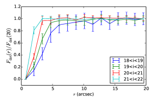
We calculate the detection efficiency $F_{\rm det}(r)$ at a distance $r$ around a particular sample of objects (e.g., bright galaxies). $F_{\rm det}(r)$ is defined as

$$F_{\rm det}(r)=\frac{\Sigma_{i}^{n}N_{i,{\rm det}}(r)}{\Sigma_{i}^{n}N_{i,{\rm true}}(r)}$$ (5)

where $i$ is summed over the $n$ objects in this sample of interest, $N_{i,{\rm det}}(r)$ is the number of objects detected at a distance $r$ and $N_{i,{\rm true}}(r)$ is the true number of objects at this distance. Without the proximity effect, we expect the $F_{\rm det}(r)$ curve to be flat.

In Figure 10 we show the $F_{\rm det}(r)$ for an arbitrary $i$-band image in our SVA1 simulations. Here we set up the calculation to estimate the detection efficiency of galaxies at $18<i<24$ in the surrounding of other galaxies in different (true) magnitude bins. For clarity, we will refer to the objects responsible for the drop in detection efficiency the “center” objects and the objects being detected the “source” objects. We would like to know how many source galaxies are missing in the magnitude range of $18<i<24$ because there is a center galaxy nearby. We find that the proximity effect is most severe in the surrounding of bright center galaxies, and the effect is seen up to several arc seconds away from the centre galaxy. In the most severe case in this test ($18<i<19$ center galaxies), the detection of the source galaxies is 50% less efficient at $\sim 4$ arcsec. For comparison, the average measured galaxy size (FLUX_RADIUS) in this image is $\sim 0.96$ arcsec.

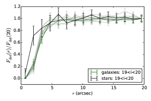
On the right panel of Figure 10 we only show the detection efficiency for the magnitude bin $19<i<20$, and overlay grey curves calculated from 10 random fields that have a range of limiting magnitude and seeing conditions. The grey curves agree well with the blue within error bars. This shows that neither cosmic variance nor seeing and limiting magnitude play a significant role in this calculation, i.e., the proximity effect is roughly at the same level for all galaxies in this magnitude bin across the sky under any observational conditions. However, if we calculate the same effect around stars in the same magnitude bin, as shown by the black curve, the shape of the curve changes and the detection efficiency increases at small separations. This is as expected since the stars have less extended profiles and are less likely to affect measurements in its surrounding pixels.

One can imagine many more similar tests using these simulations to quantify the proximity effects as a function of crowding, galaxy size and profiles etc., which would be required depending on the science analysis of interest. We will not carry out the analyses here, but only point out via the example above that by properly using simulations, one can correct for the proximity effects in the data that are otherwise difficult to estimate.

6. Conclusions

Precision cosmology in ongoing and future optical surveys critically depend on the control of systematic effects. In this generation, end-to-end simulations will play an important role in understanding these systematic effects. In this paper we describe a framework for forward-modelling the transfer function for the Dark Energy Survey (DES) that takes the astronomical sources to realistic pixel-level data products such as images and catalogs. The same framework can be adjusted for other surveys and datasets.

We use the Blind Cosmology Challenge (BCC) catalogs as the source of astronomical objects, and simulate realistic images using the Ultra Fast Image Generator (UFig). We then perform image analysis to output catalog-level products. We demonstrate the usage of this framework by forward modelling the early Science Verification (SV) data products from DES. We design the simulations and the analysis procedure to mimic closely that of the SV data, and show that our simulations reproduce many major characteristics of the data. There are small differences between the data and the simulations in certain areas of parameter spaces (e.g. small faint objects), but they can be explained by our simplified models and do not affect significantly the usage of the simulation as long as one is aware of the simplifications. By connecting the output measurement back to the input object-by-object, we have a powerful tool to investigate data-related systematic issues. We present two examples of such usage looking at star-galaxy classification and proximity effects.

This is the first implementation of such end-to-end simulation efforts for ongoing large optical surveys. In the process we have made simplifications that we understand and will improve on continuing into future work. These include (1) more sophisticated models for the source morphological distribution (2) more realistic and spatially varying models for the PSF and the background and (3) extending the current framework to also model the single-exposure images and the coadd procedure. This constantly developing simulation framework that forward models the data side-by-side as DES continues to release data, provides a powerful tool to understand and interpret data in a clean and controlled fashion. The concept can also be extended to future surveys, where the need to understand details in the data products is even more demanding.

Appendix A A. Noise level in UFig images

The noise level in images affects object detection, photometry measurements, and the completeness of the final catalog. As a result, we want to simulate images with noise properties as close as possible to that of the data. However, characterising the background level in the data is itself a challenging task, let alone the fact that we wish to model the effect of the background noise with just a simple constant Gaussian noise. In this work, we take an approximate approach using SExtractor quantities and empirically calibrate the noise level instead of deriving it from first principles. We defer a more sophisticated background model to future work.

The basic idea is that the aperture magnitude error vs. aperture magnitude relation, for large enough apertures, is only a function of the background noise. Thus, once we know this 1-1 relation as a function of background noise, we could in principle apply the appropriate background noise level to the simulations. In principle, this relation could be derived analytically and the procedure described below is unnecessary. However, since our background model includes a Lanczos resampling, this changes slightly the statistical property of the noise, complicating the relation. In addition, we want to avoid any potential nonlinear processes in SExtractor that we could be missed in the calculation.

Operationally, we calibrate the noise at the 10-$\sigma$ galaxy limiting (2 arcsec) aperture magnitude. That is, the 2 arsec aperture magnitude where the magnitude error is $\frac{2.5}{10\ln(10)}\sim$0.1086. The calibration procedure is described below:

• Generate UFig images with the median seeing of the data and a range of different background levels.

• Run SExtractor on the simulated images in the same way as on the SV data.

• Make cuts FLAGS==0 and CLASS_STAR$<$0.9 on the Source Etractor to get a clean sample of galaxies.

• Bin the galaxies in MAG_APER_4 bins of 0.01 and find the the bin where MAGERR_APER_4$\sim$0.1086, this MAG_APER_4 corresponds roughly to the 10-$\sigma$ galaxy limiting magnitude.

• For these simulations, plot the noise level vs. 2 arcsec aperture limiting magnitude and fit the relation.

In Figure 11, we show the final derived calibration curve used to convert an desired aperture limiting magnitude to a noise level we input to UFig. This calibration will change slightly for images with different seeing and source population, but at the level of accuracy ($\sim$0.02 mag) is sufficient for our purpose here.

Figure 11.— The relation between the 2 arcsec limiting aperture magnitude and the noise level in the UFig images. the blue points are the median of measurements in 10 random fields and the grey dashed line is the 4th-order polynomial fit to these data points.

References

- Agarwal et al. (2014) Agarwal, N., Ho, S., Myers, A. D., et al. 2014, JCAP, 4, 7
- Agostinelli et al. (2003) Agostinelli, S., Allison, J., Amako, K., et al. 2003, Nuclear Instruments and Methods in Physics Research A, 506, 250
- Albrecht et al. (2006) Albrecht, A., Bernstein, G., Cahn, R., et al. 2006, ArXiv Astrophysics e-prints: astro-ph/0609591, arXiv:astro-ph/0609591
- Allen et al. (2011) Allen, S. W., Evrard, A. E., & Mantz, A. B. 2011, ARA&A, 49, 409
- Amara & Réfrégier (2008) Amara, A., & Réfrégier, A. 2008, MNRAS, 391, 228
- Balbinot et al. (2012) Balbinot, E., Santiago, B., Girardi, L., et al. 2012, in Astronomical Society of the Pacific Conference Series, Vol. 461, Astronomical Data Analysis Software and Systems XXI, ed. P. Ballester, D. Egret, & N. P. F. Lorente, 287
- Becker (2013) Becker, M. R. 2013, MNRAS, 435, 115
- Behroozi et al. (2010) Behroozi, P. S., Conroy, C., & Wechsler, R. H. 2010, ApJ, 717, 379
- Bengtsson & Sjöstrand (1987) Bengtsson, H.-U., & Sjöstrand, T. 1987, Computer Physics Communications, 46, 43
- Bergé et al. (2013) Bergé, J., Gamper, L., Réfrégier, A., & Amara, A. 2013, Astronomy and Computing, 1, 23
- Beringer et al. (2012) Beringer, J., Arguin, J.-F., Barnett, R. M., et al. 2012, Phys.Rev.D, 86, 010001
- Bertin (2006) Bertin, E. 2006, in Astronomical Society of the Pacific Conference Series, Vol. 351, Astronomical Data Analysis Software and Systems XV, ed. C. Gabriel, C. Arviset, D. Ponz, & S. Enrique, 112
- Bertin (2009) Bertin, E. 2009, MemSAI, 80, 422
- Bertin (2011) Bertin, E. 2011, in Astronomical Society of the Pacific Conference Series, Vol. 442, Astronomical Data Analysis Software and Systems XX, ed. I. N. Evans, A. Accomazzi, D. J. Mink, & A. H. Rots, 435
- Bertin & Arnouts (1996) Bertin, E., & Arnouts, S. 1996, A&AS, 117, 393
- Bertin et al. (2002) Bertin, E., Mellier, Y., Radovich, M., et al. 2002, in Astronomical Society of the Pacific Conference Series, Vol. 281, Astronomical Data Analysis Software and Systems XI, ed. D. A. Bohlender, D. Durand, & T. H. Handley, 228
- Binder & Heermann (2010) Binder, K., & Heermann, D. W. 2010, Monte Carlo Simulation in Statistical Physics, doi:10.1007/978-3-642-03163-2
- Blanton et al. (2005) Blanton, M. R., Schlegel, D. J., Strauss, M. A., et al. 2005, AJ, 129, 2562
- Bouy et al. (2013) Bouy, H., Bertin, E., Moraux, E., et al. 2013, A&A, 554, A101
- Bridle et al. (2010) Bridle, S., Balan, S. T., Bethge, M., et al. 2010, MNRAS, 405, 2044
- Busha et al. (2013) Busha, M. T., Wechsler, R. H., Becker, M. R., Erickson, B., & Evrard, A. E. 2013, in American Astronomical Society Meeting Abstracts, Vol. 221, American Astronomical Society Meeting Abstracts, 341.07
- Connolly et al. (2010) Connolly, A. J., Peterson, J., Jernigan, J. G., et al. 2010, in Society of Photo-Optical Instrumentation Engineers (SPIE) Conference Series, Vol. 7738, Society of Photo-Optical Instrumentation Engineers (SPIE) Conference Series
- Conroy et al. (2006) Conroy, C., Wechsler, R. H., & Kravtsov, A. V. 2006, ApJ, 647, 201
- de Jong et al. (2013) de Jong, J. T. A., Verdoes Kleijn, G. A., Kuijken, K. H., & Valentijn, E. A. 2013, Experimental Astronomy, 35, 25
- Desai et al. (2012) Desai, S., Armstrong, R., Mohr, J. J., et al. 2012, ApJ, 757, 83
- Diehl & Dark Energy Survey Collaboration (2012) Diehl, H. T., & Dark Energy Survey Collaboration. 2012, in American Astronomical Society Meeting Abstracts, Vol. 219, American Astronomical Society Meeting Abstracts #219, #413.05
- Diehl et al. (2014) Diehl, H. T., Abbott, T. M. C., Annis, J., et al. 2014, in Society of Photo-Optical Instrumentation Engineers (SPIE) Conference Series, Vol. 9149, Society of Photo-Optical Instrumentation Engineers (SPIE) Conference Series
- Dietrich et al. (2012) Dietrich, J. P., Werner, N., Clowe, D., et al. 2012, Nature, 487, 202
- Duchon (1979) Duchon, C. E. 1979, Journal of Applied Meteorology, 18, 1016
- Fadely et al. (2012) Fadely, R., Hogg, D. W., & Willman, B. 2012, ApJ, 760, 15
- Frieman et al. (2008) Frieman, J. A., Turner, M. S., & Huterer, D. 2008, ARA&A, 46, 385
- Gerke et al. (2013) Gerke, B. F., Wechsler, R. H., Behroozi, P. S., et al. 2013, ApJS, 208, 1
- Girardi et al. (2012) Girardi, L., Barbieri, M., Groenewegen, M. A. T., et al. 2012, TRILEGAL, a TRIdimensional modeL of thE GALaxy: Status and Future, ed. A. Miglio, J. Montalbán, & A. Noels, 165
- Griffith et al. (2012) Griffith, R. L., Cooper, M. C., Newman, J. A., et al. 2012, ApJS, 200, 9
- Henrion et al. (2011) Henrion, M., Mortlock, D. J., Hand, D. J., & Gandy, A. 2011, MNRAS, 412, 2286
- Hilbert et al. (2009) Hilbert, S., Hartlap, J., White, S. D. M., & Schneider, P. 2009, A&A, 499, 31
- Ho et al. (2013) Ho, S., Agarwal, N., Myers, A. D., et al. 2013, ArXiv e-prints, arXiv:1311.2597
- Hodapp et al. (2004) Hodapp, K. W., Kaiser, N., Aussel, H., et al. 2004, Astronomische Nachrichten, 325, 636
- Huff & Graves (2014) Huff, E. M., & Graves, G. J. 2014, ApJ, 780, L16
- Huterer (2010) Huterer, D. 2010, General Relativity and Gravitation, 42, 2177
- Huterer et al. (2006) Huterer, D., Takada, M., Bernstein, G., & Jain, B. 2006, MNRAS, 366, 101
- Jouvel et al. (2009) Jouvel, S., Kneib, J.-P., Ilbert, O., et al. 2009, A&A, 504, 359
- Kiessling et al. (2011) Kiessling, A., Heavens, A. F., Taylor, A. N., & Joachimi, B. 2011, MNRAS, 414, 2235
- Kitching et al. (2012) Kitching, T. D., Balan, S. T., Bridle, S., et al. 2012, MNRAS, 423, 3163
- Kron (1980) Kron, R. G. 1980, ApJS, 43, 305
- Leistedt et al. (2013) Leistedt, B., Peiris, H. V., Mortlock, D. J., Benoit-Lévy, A., & Pontzen, A. 2013, MNRAS, 435, 1857
- Lin et al. (2010) Lin, H., Kuropatkin, N., Wechsler, R., et al. 2010, in Bulletin of the American Astronomical Society, Vol. 42, American Astronomical Society Meeting Abstracts 215, 470.07
- Maddox et al. (2012) Maddox, N., Hewett, P. C., Péroux, C., Nestor, D. B., & Wisotzki, L. 2012, MNRAS, 424, 2876
- Marchesini et al. (1992) Marchesini, G., Webber, B. R., Abbiendi, G., et al. 1992, Computer Physics Communications, 67, 465
- Melchior et al. (2014) Melchior, P., Suchyta, E., Huff, E., et al. 2014, ArXiv e-prints, arXiv:1405.4285
- Miyazaki et al. (2012) Miyazaki, S., Komiyama, Y., Nakaya, H., et al. 2012, in Society of Photo-Optical Instrumentation Engineers (SPIE) Conference Series, Vol. 8446, Society of Photo-Optical Instrumentation Engineers (SPIE) Conference Series
- Moffat (1969) Moffat, A. F. J. 1969, A&A, 3, 455
- Mohr et al. (2012) Mohr, J. J., Armstrong, R., Bertin, E., et al. 2012, in Society of Photo-Optical Instrumentation Engineers (SPIE) Conference Series, Vol. 8451, Society of Photo-Optical Instrumentation Engineers (SPIE) Conference Series
- Nelson & Namito (1990) Nelson, W. R., & Namito, Y. 1990, in Presented at the International Conference on Supercomputing in Nuclear Applications, Mito City, Japan, 12-16 Mar. 1990, 12–16
- Ngeow et al. (2006) Ngeow, C., Mohr, J. J., Alam, T., et al. 2006, in Society of Photo-Optical Instrumentation Engineers (SPIE) Conference Series, Vol. 6270, Society of Photo-Optical Instrumentation Engineers (SPIE) Conference Series, 23
- Peng et al. (2002) Peng, C. Y., Ho, L. C., Impey, C. D., & Rix, H.-W. 2002, AJ, 124, 266
- Peterson & Jernigan (2013) Peterson, J. R., & Jernigan, J. G. 2013, phoSim: Photon Simulator, Astrophysics Source Code Library, ascl:1307.011
- Pollo et al. (2010) Pollo, A., Rybka, P., & Takeuchi, T. T. 2010, A&A, 514, A3
- Riebe et al. (2013) Riebe, K., Partl, A. M., Enke, H., et al. 2013, Astronomische Nachrichten, 334, 691
- Ross et al. (2012) Ross, A. J., Percival, W. J., Sánchez, A. G., et al. 2012, MNRAS, 424, 564
- Rossetto et al. (2011) Rossetto, B. M., Santiago, B. X., Girardi, L., et al. 2011, AJ, 141, 185
- Ruiz-Lapuente (2014) Ruiz-Lapuente, P. 2014, Dark Energy
- Scolnic et al. (2014) Scolnic, D., Rest, A., Riess, A., et al. 2014, ApJ, 795, 45
- Sérsic (1963) Sérsic, J. L. 1963, Boletin de la Asociacion Argentina de Astronomia La Plata Argentina, 6, 41
- Sevilla et al. (2011) Sevilla, I., Armstrong, R., Bertin, E., et al. 2011, ArXiv e-prints, arXiv:1109.6741
- Smith et al. (2008) Smith, B., Sigurdsson, S., & Abel, T. 2008, MNRAS, 385, 1443
- Soumagnac et al. (2013) Soumagnac, M. T., Abdalla, F. B., Lahav, O., et al. 2013, ArXiv e-prints, arXiv:1306.5236
- Springel & Hernquist (2003) Springel, V., & Hernquist, L. 2003, MNRAS, 339, 289
- The Dark Energy Survey Collaboration (2005) The Dark Energy Survey Collaboration. 2005, ArXiv Astrophysics e-prints: astro-ph/0510346, arXiv:astro-ph/0510346
- Vogelsberger et al. (2012) Vogelsberger, M., Sijacki, D., Kereš, D., Springel, V., & Hernquist, L. 2012, MNRAS, 425, 3024
- Weinberg et al. (2013) Weinberg, D. H., Mortonson, M. J., Eisenstein, D. J., et al. 2013, Physics Reports, 530, 87
- White et al. (2013) White, M., Tinker, J. L., & McBride, C. K. 2013, MNRAS, arXiv:1309.5532
- Zhang et al. (2014) Zhang, Y., McKay, T. A., Bertin, E., et al. 2014, ArXiv e-prints, arXiv:1409.2885