MIFPA-14-31

We study non-supersymmetric truncations of $\omega$-deformed ${\cal N}=8$ gauged supergravity that retain a $U(1)$ gauge field and three scalars, of which two are neutral and one charged. We construct dyonic domain-wall and black hole solutions with AdS₄ boundary conditions when only one (neutral) scalar is non-vanishing, and examine their behavior as the magnetic field and temperature of the system are varied. In the infrared the domain-wall solutions approach either dyonic AdS${}_{2}\times\mathbb{R}^{2}$ or else Lifshitz-like, hyperscaling violating geometries. The scaling exponents of the latter are $z=3/2$ and $\theta=-2$, and are independent of the $\omega$-deformation. New $\omega$-dependent AdS₄ vacua are also identified. We find a rich structure for the magnetization of the system, including a line of metamagnetic first-order phase transitions when the magnetic field lies in a particular range. Such transitions arise generically in the $\omega$-deformed theories. Finally, we study the onset of a superfluid phase by allowing a fluctuation of the charged scalar field to condense, spontaneously breaking the abelian gauge symmetry. The mechanism by which the superconducting instability ceases to exist for strong magnetic fields is different depending on whether the field is positive or negative. Finally, such instabilities are expected to compete with spatially modulated phases.

1 Introduction

Holographic techniques have recently been applied to probe novel phases of matter and materials whose unconventional behavior is tied to strong coupling, and is therefore poorly understood. In turn these efforts have led to the discovery of new classes of gravitational solutions and instabilities, hinting at a rich structure of infrared (IR) phases. We have seen the emergence of vacua characterized by a number of broken symmetries, and scaling geometries that incorporate a dynamical critical exponent and hyperscaling violation, an anomalous scaling of the free energy. There is a program under way to classify such solutions and to understand how they might arise via renormalization group (RG) flow from an ultraviolet (UV) CFT. Bottom-up gravitational models have been used to generate a variety of these systems. Top-down models have then served as a concrete framework for testing these ideas, confirming many of the features observed in the bottom-up constructions, and giving insight into the competition between different phases.

In this paper we shall work with a non-supersymmetric but consistent truncation of the newly discovered one-parameter family of inequivalent ${\cal N}=8$ gauged $SO(8)$ supergravities. The ${\cal N}=8$ supergravities are characterized by a real parameter $\omega$ that lies in the range $0\leq\omega\leq\pi/8$ [1, 2]. The non-supersymmetric truncation we shall consider was previously studied in [3] as a certain $SO(4)$-invariant truncation of the standard [4] undeformed ${\cal N}=8$ theory (it was called the $SO(4)^{\prime}$ truncation in [3]). The truncation involves setting to zero certain scalar fields that play a role in restricting the range of inequivalent values of the $\omega$ parameter in the deformed ${\cal N}=8$ theory, and in fact after the truncation it turns out that the range of $\omega$ for inequivalent theories is extended to $0\leq\omega\leq\pi/4$. When $\omega=0$ the truncated theory can, of course, be obtained as a truncation of the dimensional reduction of eleven-dimensional supergravity on a seven-dimensional sphere, since the latter gives rise to the standard $\omega=0$ supergravity. On the other hand, the $\omega=\pi/4$ truncated theory can be obtained via a reduction from eleven-dimensions on a seven-dimensional Sasaki-Einstein manifold [5]. The higher-dimensional origin of the general $\omega$-deformed theories, and in particular, whether they can be embedded in eleven dimensions, is still not understood (see [2] for a discussion).

The truncation we consider here retains a $U(1)$ gauge field and three scalars, of which two are neutral and one charged. The $\omega$-deformation parameter controls the couplings of the scalars to the gauge field, and also the structure of the scalar potential. We shall choose the form of the gauge field so that the $(2+1)$ dimensional UV CFT is at finite density, with chemical potential $\mu$ and magnetic field $B$, and then examine the possible ground states of the theory. Throughout the paper our main interest will be in a further truncation of the system in which only one of the neutral scalars is retained. When the charged scalar field is also set to zero it is straightforward to construct numerically solutions both at zero and at non-zero temperatures, and to examine their properties as one varies the magnetic field and temperature in the system.

As we shall see, the behavior of the $\omega$-deformed black holes is highly sensitive to the strength of the magnetic field. Depending on $|B|$, as $T\rightarrow 0$ the IR geometry will approach either a dyonic AdS${}_{2}\times\mathbb{R}^{2}$ or a solution exhibiting hyperscaling violation and Lifshitz-like scaling. For the latter the dynamical critical exponent and the hyperscaling violating exponent are, respectively, $z=3/2$ and $\theta=-2$, independent of the value of the $\omega$ parameter because of the particular structure of the gauge coupling and scalar potential. When the magnetic field lies within a certain range, the thermodynamically preferred black hole solutions will jump between branches that have different IR behaviors as the temperature is changed. This transition will then give rise to a sudden jump in the magnetization of the system, resulting in (a line of) first order metamagnetic phase transitions. The latter will eventually end at a critical point – where the phase transition becomes second-order or higher – when the magnetic field is tuned to a particular critical value. Metamagnetic transitions of this type occur in a variety of materials, including rare earth and transition metals and strongly correlated electron systems. Holographic studies of metamagnetism have appeared in [10, 11, 12, 13]. Here we will follow closely the analysis of [13], which corresponds to $\omega=\pi/4$ in our construction. Finally, when the black holes are cooled down to zero temperature, they become dyonic domain-wall solutions interpolating between AdS₄ in the UV and the two types of IR geometries that we just described. In particular, when the deep IR is AdS${}_{2}\times\mathbb{R}^{2}$, the system exhibits either paramagnetism or diamagnetism depending on the value of $B$. Interestingly, for certain choices of $\omega$ the magnetic field can be tuned so that the system will go from being paramagnetic to diamagnetic, within the same thermodynamically preferred branch.

The well-known extensive zero temperature entropy associated with AdS${}_{2}\times\mathbb{R}^{2}$ suggests that the latter should not describe – generically – the true ground state of the system. Rather, one expects the corresponding black holes to suffer from instabilities at sufficiently low temperatures, leading to the formation of new phases. In the extremal geometry, such instabilities would be signaled by the existence of tachyonic modes violating the Breitenlöhner-Freedman (BF) bound for AdS₂. Indeed, in the theories we are considering the charged scalar field can condense, spontaneously breaking the $U(1)$ symmetry and triggering a superfluid instability as in [14, 15, 16]. Towards the end of the paper we shall study the onset of this instability in a limit in which the scalar does not back react on the geometry. In particular, we shall determine the critical temperature at which the instability sets in, and how it depends on the value of the magnetic field. When $B<0$, we shall see that the charged scalar stops condensing when the field reaches a sufficiently large value, consistent with the Meissner effect. On the other hand, for $B>0$ the instability will stop only when the thermodynamically preferred black hole background is hyperscaling-violating in the IR. The asymmetry between positive and negative values of $B$ is generic for the $\omega$-deformations of the $\omega=0$ theory. In an appropriate range of values for $B$, we also expect to find spatially modulated instabilities – hinting at the presence of striped phases – which are well known to be associated with geometries with an IR AdS${}_{2}\times\mathbb{R}^{2}$ description [17, 18, 19, 20]. Indeed, striped phases have been experimentally observed to compete with superconductivity in e.g. certain high $T_{c}$ superconductors [21]. We shall discuss briefly the range in which we expect spatially modulated instabilities to be present and possibly dominate over the superfluid phase, and leave a more detailed analysis to future work.

Finally, we should mention that the truncations of the $\omega$-deformed theories that we are considering in this paper also admit new AdS₄ vacua. These have linearized instabilities within the the full $SO(4)^{\prime}$ truncation, resulting from the occurrence of scalar flucuations whose masses lie below the Breitenlöhner-Freedman bound. In one of the new AdS₄ vacua there is a single such unstable mode, and the associated scalar could in fact itself be consistently truncated, leaving a stable AdS₄ solution of the further-truncated theory. It would be interesting to construct domain-wall geometries which interpolate between two AdS₄ fixed points, along the lines of [22, 23]. Moreover, given the structure of the scalar potential and gauge couplings in our truncation – and in particular, the fact that they generically give rise to hyperscaling violating solutions – we wonder whether there may be some overlap with the construction of [24], where the intermediate geometry was associated with a scaling regime. We leave these questions to future work.

The outline of the paper is as follows. Section 2 introduces the truncation we shall work with, and the relevant equations of motion, while Section 3 describes the geometries that arise in the IR. In Section 4 we discuss the thermodynamics and construct numerically the dyonic black hole solutions of the theory. We focus on the behavior of the free energy and magnetization as a function of temperature. In Section 5 we cool down our dyonic black hole solutions and describe properties of the resulting domain-wall solutions. We analyze superfluid instabilities triggered by the condensation of the charged scalar field in Section 6, and discuss the competition with striped phases. Concluding remarks are relegated to Section 7. Finally, Appendix A contains a brief discussion of the duality rotation one can perform in the theory, while Appendix B contains a description of new AdS₄ vacua together with a linearized stability analysis.

2 Non-supersymmetric $\omega$-deformed truncation

In this paper we shall study a theory obtained from the $\omega$-deformed ${\cal N}=8$ gauged supergravity by first performing a consistent truncation to an $SO(4)$-invariant subsector of the $SO(8)$ gauged supergravity. This truncation, referred to as the $SO(4)^{\prime}$-invariant theory in [3], can be described conveniently in the symmetric gauge, where the $E_{7}/SU(8)$ scalar coset representative of the $SO(8)$ gauged theory is parameterised as

$${\cal V}=\exp\begin{pmatrix}0&-{\frac{1}{2\sqrt{2}}}\phi_{ijk\ell}\cr-{\frac{1}{2\sqrt{2}}}\phi^{mnpq}&0\end{pmatrix}\,,$$ (2.1)

where $\phi^{ijk\ell}$ are complex scalar fields, totally antisymmetric in the rigid $SU(8)$ indices, and obeying the complex self-duality constraint

$$\phi_{ijk\ell}={\frac{1}{4!}}\,\varepsilon_{ijk\ell mnpq}\,\phi^{mnpq}\,.$$ (2.2)

Note that in the symmetric gauge $SU(8)$ and $SO(8)$ indices are identified. Introducing coordinates $x^{i}$ on ${\mathbb{R}}^{8}$, the 35 complex scalar fields can be written as

$$\Phi={\frac{1}{4!}}\,\phi_{ijk\ell}dx^{i}\wedge dx^{j}\wedge dx^{k}\wedge dx^{\ell}\,.$$ (2.3)

The truncation to the $SO(4)^{\prime}$-invariant subsector is described in detail in section 6 of reference [3]. For our purposes it is convenient to view the ${\mathbb{R}}^{8}$ introduced above as ${\mathbb{C}}^{4}$, with complex coordinates defined by

$$z^{1}=x^{1}+{{\rm i}}x^{3}\,,\quad z^{2}=x^{2}+{{\rm i}}x^{4}\,,\quad z^{3}=x^{5}+{{\rm i}}x^{7}\,,\quad z^{4}=x^{6}+{{\rm i}}x^{8}\,.$$ (2.4)

The $SO(4)^{\prime}$-invariant truncation in [3], which retains six real scalar fields that we shall parameterise as $(\lambda_{0},x,\rho,\chi,\lambda_{4},\lambda_{5})$, is then given by

$$\Phi = -{\frac{\lambda_{0}}{8\sqrt{3}}}\,dz^{\alpha}\wedge dz^{\beta}\wedge d\bar{z}^{\alpha}\wedge d\bar{z}^{\beta}+{\frac{x}{16}}\,\varepsilon_{\alpha\beta\gamma\delta}\,dz^{\alpha}\wedge dz^{\beta}\wedge d\bar{z}^{\gamma}\wedge d\bar{z}^{\delta}$$ (2.5)

$$+{\frac{\rho}{4}}\,\Big{[}e^{{{\rm i}}\chi}\,dz^{1}\wedge dz^{2}\wedge dz^{3}\wedge dz^{4}+\hbox{c.c}\Big{]}$$

$$+{\frac{1}{48}}\Big{[}(\lambda_{4}+{{\rm i}}\lambda_{5})\,\varepsilon_{\alpha\beta\gamma\delta}\,dz^{\alpha}\wedge dz^{\beta}\wedge dz^{\gamma}\wedge d\bar{z}^{\delta}+\hbox{c.c}\Big{]}\,.$$

Note that the $SO(4)^{\prime}$ symmetry is contained within the $SU(4)$ that acts on ${\mathbb{C}}^{4}$, and so it preserves not only the $SU(4)$ invariants $\delta_{\alpha\bar{\beta}}$, $\varepsilon_{\alpha\beta\gamma\delta}$ and $\varepsilon_{\bar{\alpha}\bar{\beta}\bar{\gamma}\bar{\delta}}$ of complex geometry but also $\delta_{\alpha\beta}$ and $\delta_{\bar{\alpha}\bar{\beta}}$. Thus we do not need to distinguished between barred and unbarred indices in the expression (2.5) for $\Phi$, which is $SO(4)^{\prime}$-invariant but not $SU(4)$-invariant.

There is just a single $U(1)$ gauge symmetry that commutes with $SO(4)^{\prime}$, namely the $U(1)$ factor in the $U(4)=SU(4)\times U(1)$ that acts on ${\mathbb{C}}^{4}$. The surviving gauge field $A_{\mu}$ is embedded within the original 28 gauge fields $A_{\mu}^{IJ}$ of $SO(8)$ as

$${\textstyle{\frac{\scriptstyle 1}{\scriptstyle 2}}}A_{\mu}^{IJ}dx^{I}\wedge dx^{J}={\frac{{{\rm i}}}{2}}\,A_{\mu}\,dz^{\alpha}\wedge d\bar{z}^{\alpha}\,.$$ (2.6)

We can equivalently express the embedding of the gauge file as

$$A^{IJ}_{\mu}=A_{\mu}(\sigma_{0}\otimes{\rm i}\sigma_{2}\otimes\sigma_{0})^{IJ}\,.$$ (2.7)

It is evident from (2.6) that the charges of the remaining fields under the residual $U(1)$ gauge symmetry are proportional to $(n-\bar{n})$, where $n$ and $\bar{n}$ count the number of holomorphic and anti-holomorphic coordinate differentials $dz^{\alpha}$ and $d\bar{z}^{\alpha}$ in their expansions as differential forms in ${\mathbb{C}}^{4}$. Normalising the charges to be $Q={\textstyle{\frac{\scriptstyle 1}{\scriptstyle 2}}}(n-\bar{n})$, we see from (2.5) that the scalars $\lambda_{0}$ and $x$ are uncharged; $\rho e^{{{\rm i}}\chi}$ describes a complex scalar with charge 2 and $(\lambda_{4}+{{\rm i}}\lambda_{5})$ describes a complex scalar of charge 1.

With these charge assignments we see that we can make a further consistent truncation in which we set

$$\lambda_{4}=\lambda_{5}=0\,,$$ (2.8)

since retained fields with charges 0 and $\pm 2$ can never act as sources for fields of charge $\pm 1$. In terms of the notation in section 6 of [3], where the scalar fields in the $SO(4)^{\prime}$-invariant truncation were denoted by $(\lambda_{0},\lambda_{1},\lambda_{2},\lambda_{3},\lambda_{4},\lambda_{5})$, the four scalars $(\sigma,x,\rho,\chi)$ that we are retaining correspond to

$$\lambda_{0}=\sigma\,,\quad\lambda_{1}={\textstyle{\frac{\scriptstyle\sqrt{3}}{\scriptstyle 2}}}\,(x-\rho\cos\chi)\,,\quad\lambda_{2}=\rho\sin\chi\,,\quad\lambda_{3}={\textstyle{\frac{\scriptstyle 1}{\scriptstyle 2}}}(3x+\rho\cos\chi)\,.$$ (2.9)

Having obtained the form of the scalar 56-bein ${\cal V}$ for the consistent truncation we are considering, it is a mechanical, if somewhat involved, procedure to substitute it into the expressions given in [2] for the various terms in the Lagrangian of the $\omega$-deformed ${\cal N}=8$ gauged supergravity. We find that the $\omega$-deformed scalar potential is given by

$$V=-f(R,x,\rho)\,\cos^{2}\omega-f(R^{-1},x,\rho)\,\sin^{2}\omega\,,$$ (2.10)

where

$$f={\textstyle{\frac{\scriptstyle 3}{\scriptstyle 4}}}g^{2}R^{-1}\,(\cosh 2x+3)+3g^{2}R\,\cosh x\,\cosh\rho-{\textstyle{\frac{\scriptstyle 1}{\scriptstyle 2}}}g^{2}R^{3}\,\sinh^{2}\rho\,,$$ (2.11)

and we have also defined

$$R=e^{-\sigma/\sqrt{3}}\,.$$ (2.12)

The scalar kinetic terms are constructed as $-{\textstyle{\frac{\scriptstyle 1}{\scriptstyle 48}}}{\cal A}_{\mu}^{ijk\ell}{\cal A}^{\mu}_{ijk\ell}$, where ${\cal A}_{\mu}^{ijk\ell}$ is given by [2]

$$D_{\mu}{\cal V}\,{\cal V}^{-1}=-{\frac{1}{2\sqrt{2}}}\,\begin{pmatrix}0&{\cal A}_{\mu}^{ijk\ell}\cr{\cal A}_{\mu\,ijk\ell}&0\end{pmatrix}\,.$$ (2.13)

The $SO(8)$ gauged covariant derivative of the scalar coset is defined as

$${\cal D}_{\mu}u_{ij}^{~{}~{}IJ}=\partial_{\mu}u_{ij}^{~{}~{}IJ}-{\textstyle{\frac{\scriptstyle 1}{\scriptstyle 2}}}{\cal B}_{\mu~{}i}^{k}u_{kj}^{~{}~{}IJ}-{\textstyle{\frac{\scriptstyle 1}{\scriptstyle 2}}}{\cal B}_{\mu~{}j}^{k}u_{ik}^{~{}~{}IJ}-g(A_{\mu}^{KI}u_{ij}^{~{}~{}JK}-A_{\mu}^{KJ}u_{ij}^{~{}~{}IK})\,,$$ (2.14)

where ${\textstyle{\frac{\scriptstyle 1}{\scriptstyle 2}}}{\cal B}_{~{}j}^{i}$ is the composite SU(8) connection and is determined by requiring that (2.13) hold. Plugging in the ansatz, we obtain

$$e^{-1}{\cal L}_{\rm kin}=-{\textstyle{\frac{\scriptstyle 1}{\scriptstyle 2}}}({\partial}\rho)^{2}-{\textstyle{\frac{\scriptstyle 1}{\scriptstyle 2}}}\sinh^{2}\rho\,({\partial}\chi-2gA)^{2}-{\textstyle{\frac{\scriptstyle 1}{\scriptstyle 2}}}({\partial}\sigma)^{2}-{\textstyle{\frac{\scriptstyle 3}{\scriptstyle 2}}}({\partial}x)^{2}\,.$$ (2.15)

The kinetic term of the $U(1)$ gauge field is given by

$$e^{-1}{\cal L}_{F} = -\Big{(}\frac{e^{\sqrt{3}\sigma}\cos\omega-{\rm i}\sin\omega}{\cos\omega-{\rm i}e^{\sqrt{3}\sigma}\sin\omega}F^{+\mu\nu}F^{+}_{\mu\nu}+{\rm h.c.}\Big{)}$$ (2.16)

$$= -U(\sigma)\,F^{\mu\nu}F_{\mu\nu}-W(\sigma)\,F^{\mu\nu}\,{{}^{*}\!F}_{\mu\nu}\,,$$

with the gauge kinetic couplings taking the form

$$U(\sigma)=\frac{1}{\cosh\sqrt{3}\sigma-\cos 2\omega\sinh\sqrt{3}\sigma}\,,\qquad W(\sigma)=\frac{\sin 2\omega\sinh\sqrt{3}\sigma}{\cosh\sqrt{3}\sigma-\cos 2\omega\sinh\sqrt{3}\sigma}\,.$$ (2.17)

Combining the ingredients above, the bosonic Lagrangian for our system becomes

$$\mathcal{L}= - {\textstyle{\frac{\scriptstyle 1}{\scriptstyle 2}}}({\partial}\rho)^{2}-{\textstyle{\frac{\scriptstyle 1}{\scriptstyle 2}}}\sinh^{2}\rho\,({\partial}\chi-2gA)^{2}-{\textstyle{\frac{\scriptstyle 1}{\scriptstyle 2}}}({\partial}\sigma)^{2}-{\textstyle{\frac{\scriptstyle 3}{\scriptstyle 2}}}({\partial}x)^{2}$$ (2.18)

$$- U(\sigma)\,F^{\mu\nu}F_{\mu\nu}-W(\sigma)\,F^{\mu\nu}\,{{}^{*}\!F}_{\mu\nu}-V(\sigma,x,\rho)\,,$$

with the scalar potential given by

$$V = -3g^{2}[{\textstyle{\frac{\scriptstyle 1}{\scriptstyle 4}}}e^{\,\sigma/\sqrt{3}}\,(\cosh 2x+3)+e^{-\sigma/\sqrt{3}}\,\cosh x\,\cosh\rho-{\textstyle{\frac{\scriptstyle 1}{\scriptstyle 6}}}e^{-3\sigma/\sqrt{3}}\,\sinh^{2}\rho]\cos^{2}\omega$$ (2.19)

$$- 3g^{2}[{\textstyle{\frac{\scriptstyle 1}{\scriptstyle 4}}}e^{-\sigma/\sqrt{3}}\,(\cosh 2x+3)+e^{\,\sigma/\sqrt{3}}\,\cosh x\,\cosh\rho-{\textstyle{\frac{\scriptstyle 1}{\scriptstyle 6}}}e^{3\sigma/\sqrt{3}}\,\sinh^{2}\rho]\sin^{2}\omega\,.$$

Notice that when $x=\rho=0$ the entire $\omega$-dependence drops out of the scalar potential. There is still, however, $\omega$-dependence in the coupling of the scalar field $\sigma$ to the gauge field kinetic terms.

It is important to establish the range of the deformation parameter $\omega$ that characterises inequivalent theories. In the full ${\cal N}=8$ gauged supergravity, one can see that each value of $\omega$ in the line interval $0\leq\omega\leq\pi/8$ describes an inequivalent theory [1, 2]. As is discussed there in detail, there is a symmetry under $\omega\rightarrow\omega+\pi/2$, under which certain scalar fields undergo sign reversal transformations. There is also a symmetry under $\omega\rightarrow-\omega$, combined with a parity reversal. These two symmetries alone would imply that inequivalent theories would correspond to points in the line interval $0\leq\omega\leq\pi/4$. However there is also another rather more subtle symmetry in the ${\cal N}=8$ theory, under the translation $\omega\rightarrow\omega+\pi/4$ [2]. This symmetry requires making phase transformations of some of the (complex) scalar fields. It is this symmetry, combined with $\omega\rightarrow-\omega$, that results in the $0\leq\omega\leq\pi/8$ interval for inequivalent ${\cal N}=8$ theories. In the truncation that we are making, the imaginary parts of some of the complex scalars of the original ${\cal N}=8$ theory are set to zero. In particular, we have the real scalar field $\sigma$ that is retained in the truncation. As a consequence, it is no longer possible to implement the required complex phase transformations on the retained fields that would compensate the translation $\omega\rightarrow\omega+\pi/4$. The upshot is that the interval of $\omega$ corresponding to inequivalent theories in the truncations we are considering here is

$$0\leq\omega\leq{\frac{\pi}{4}}\,.$$ (2.20)

Note that one can indeed see from the gauge-field kinetic terms given by (2.16) and (2.17) that the theory with $\omega=\pi/4$ is inequivalent to the theory with $\omega=0$.

Finally, the equations of motion following from (2.18) are

$$\square\,\rho = \sinh\rho\,\cosh\rho\,({\partial}\chi-2gA)^{2}+{\frac{{\partial}V}{{\partial}\rho}}\,,$$

$$\square\,\sigma = {\frac{{\partial}V}{{\partial}\sigma}}+{\frac{{\partial}U}{{\partial}\sigma}}\,F^{\mu\nu}F_{\mu\nu}+{\frac{{\partial}W}{{\partial}\sigma}}\,F^{\mu\nu}\,{{}^{*}\!F}_{\mu\nu}\,,\qquad\square\,x=\frac{1}{3}{\frac{{\partial}V}{{\partial}x}}\,,$$

$$0 = \nabla^{\mu}\Big{(}\sinh^{2}\rho\,({\partial}_{\mu}\chi-2gA_{\mu})\Big{)}\,,$$

$$0 = \nabla^{\mu}\Big{(}U(\sigma)\,F_{\mu\nu}+W(\sigma)\,{{}^{*}\!\,F}_{\mu\nu}\Big{)}+\frac{g}{2}\sinh^{2}\rho\,({\partial}_{\nu}\chi-2gA_{\nu})\,,$$

$$R_{\mu\nu} = {\textstyle{\frac{\scriptstyle 1}{\scriptstyle 2}}}{\partial}_{\mu}\rho{\partial}_{\nu}\rho+{\textstyle{\frac{\scriptstyle 1}{\scriptstyle 2}}}{\partial}_{\mu}\sigma{\partial}_{\nu}\sigma+{\textstyle{\frac{\scriptstyle 3}{\scriptstyle 2}}}{\partial}_{\mu}x{\partial}_{\nu}x+{\textstyle{\frac{\scriptstyle 1}{\scriptstyle 2}}}\sinh^{2}\rho\,({\partial}_{\mu}\chi-2gA_{\mu})({\partial}_{\nu}\chi-2gA_{\nu})$$ (2.21)

$$+2U(\sigma)\,(F_{\mu\rho}F_{\nu}^{\;\;\rho}-{\textstyle{\frac{\scriptstyle 1}{\scriptstyle 4}}}F^{2}\,g_{\mu\nu})+{\textstyle{\frac{\scriptstyle 1}{\scriptstyle 2}}}V\,g_{\mu\nu}\,.$$

2.1 Restricting to two scalar fields

In the $\omega$-deformed theories discussed above it is consistent to set the neutral scalar field $x$ to zero and retain only $\sigma$ and the charged scalar field $\rho\,e^{\,i\chi}$. Moreover, for the cases we will consider the gauge choice $\nabla^{\mu}A_{\mu}=0$ allows to set the phase $\chi$ to zero. With $x=\chi=0$ and $\nabla^{\mu}A_{\mu}=0$, the equations of motion become

$$\square\rho = 4g^{2}\sinh\rho\,\cosh\rho\,A^{2}+{\frac{{\partial}V}{{\partial}\rho}}\,,$$

$$\square\sigma = {\frac{{\partial}V}{{\partial}\sigma}}+{\frac{{\partial}U}{{\partial}\sigma}}\,F^{\mu\nu}F_{\mu\nu}+{\frac{{\partial}W}{{\partial}\sigma}}\,F^{\mu\nu}\,{{}^{*}\!F}_{\mu\nu}\,,$$

$$0 = \nabla^{\mu}\Big{(}U(\sigma)\,F_{\mu\nu}+W(\sigma)\,{{}^{*}\!\,F}_{\mu\nu}\Big{)}-g^{2}\sinh^{2}\rho\,A_{\nu}\,,$$

$$R_{\mu\nu} = {\textstyle{\frac{\scriptstyle 1}{\scriptstyle 2}}}{\partial}_{\mu}\rho{\partial}_{\nu}\rho+{\textstyle{\frac{\scriptstyle 1}{\scriptstyle 2}}}{\partial}_{\mu}\sigma{\partial}_{\nu}\sigma+2g^{2}\sinh^{2}\rho\,A_{\mu}A_{\nu}$$ (2.22)

$$+2\,U(\sigma)\,(F_{\mu\rho}F_{\nu}^{\;\;\rho}-{\textstyle{\frac{\scriptstyle 1}{\scriptstyle 4}}}F^{2}\,g_{\mu\nu})+{\textstyle{\frac{\scriptstyle 1}{\scriptstyle 2}}}V\,g_{\mu\nu}\,,$$

where the scalar potential depends on the $\omega$-deformation through

$$V = -3g^{2}[e^{\,\sigma/\sqrt{3}}+e^{-\sigma/\sqrt{3}}\,\cosh\rho-{\textstyle{\frac{\scriptstyle 1}{\scriptstyle 6}}}e^{-\sqrt{3}\,\sigma}\,\sinh^{2}\rho]\cos^{2}\omega$$ (2.23)

$$- 3g^{2}[e^{-\sigma/\sqrt{3}}+e^{\,\sigma/\sqrt{3}}\,\cosh\rho-{\textstyle{\frac{\scriptstyle 1}{\scriptstyle 6}}}e^{\sqrt{3}\,\sigma}\,\sinh^{2}\rho]\sin^{2}\omega\,.$$

Again, notice that the $\omega$-dependence cancels when $\rho=0$.

2.1.1 Domain-wall and black hole ansatz

We conclude this section with the particular background ansatz which will be convenient for studying domain-wall and black hole solutions in the rest of the paper. We take the background to be given by

$$ds^{2} = -e^{-\beta(r)}f(r)dt^{2}+\frac{dr^{2}}{f(r)}+r^{2}d\vec{x}^{2}\,,$$

$$A = \phi(r)\,dt+{\textstyle{\frac{\scriptstyle 1}{\scriptstyle 2}}}B(xdy-ydx)\,,\qquad\sigma=\sigma(r)\,,$$ (2.24)

for which we have

$$A^{2} = \frac{B^{2}}{4r^{2}}(x^{2}+y^{2})-\frac{e^{\beta}\phi^{2}}{f}\,,\quad F^{2}=\frac{2B^{2}}{r^{4}}-2e^{\beta}\phi^{\prime\;2}\,,\quad F^{\mu\nu}\,{{}^{*}\!F}_{\mu\nu}=\frac{4\,e^{\beta/2}}{r^{2}}B\phi^{\prime}\,.$$ (2.25)

The scalar equations of motion then take the form

$$\square\,\rho = 4g^{2}\sinh\rho\,\cosh\rho\,\left[\frac{B^{2}}{4r^{2}}(x^{2}+y^{2})-\frac{e^{\beta}\phi^{2}}{f}\right]+{\frac{{\partial}V}{{\partial}\rho}}\,,$$

$$\square\,\sigma = {\frac{{\partial}V}{{\partial}\sigma}}+\left[\frac{2B^{2}}{r^{4}}-2e^{\beta}\phi^{\prime\;2}\right]\,{\frac{{\partial}U}{{\partial}\sigma}}+\left[\frac{4\,e^{\beta/2}}{r^{2}}B\phi^{\prime}\right]{\frac{{\partial}W}{{\partial}\sigma}}\,,$$ (2.26)

while the gauge field equations of motion become

$$0 = fU\phi^{\prime\prime}+\phi^{\prime}[fU^{\prime}+{\textstyle{\frac{\scriptstyle 1}{\scriptstyle 2}}}fU\beta^{\prime}+\frac{2}{r}fU]-g^{2}\sinh\rho^{2}\phi^{2}-\frac{f}{e^{\beta/2}r^{2}}BW^{\prime}\,,$$ (2.27)

$$0 = -\frac{B}{2}g^{2}\,y\,\sinh\rho^{2}\,,$$ (2.28)

$$0 = \frac{B}{2}g^{2}\,x\,\sinh\rho^{2}\,,$$ (2.29)

where $U^{\prime}=\frac{\partial U}{\partial\sigma}\frac{\partial\sigma}{\partial r}$ and similarly $W^{\prime}=\frac{\partial W}{\partial\sigma}\frac{\partial\sigma}{\partial r}$.

It is apparent that the choice $\rho=0$ is consistent with the equations above, and in particular with (2.28) and (2.29) when $B\neq 0$. Notice that these two equations can also be satisfied by working to linear order in perturbations of $\rho$,

$$\rho=\bar{\rho}+\delta\rho\,,$$ (2.30)

assuming that the background value is $\bar{\rho}=0$. The remaining equation (2.27) then fixes $\phi$. Finally, the diagonal components of Einstein’s equations are given by

$$f\beta^{\prime\prime}-f^{\prime\prime}+2\left[\frac{3}{4}f^{\prime}\beta^{\prime}+\frac{f\beta^{\prime}}{r}-{\textstyle{\frac{\scriptstyle 1}{\scriptstyle 4}}}\beta^{\prime\;2}f-\frac{f^{\prime}}{r}\right]=V-2U\left[e^{\beta}\phi^{\prime\;2}+\frac{B^{2}}{r^{4}}\right]-4g^{2}\frac{e^{\beta}\sinh\rho^{2}}{f}\,,$$

$$\rho^{\prime\,2}+\sigma^{\prime\,2}+\frac{2\beta^{\prime}}{r}+4g^{2}\frac{e^{\beta}\sinh\rho^{2}}{f^{2}}\phi^{2}=0\,,$$

$$\frac{1}{r^{2}}\left[2f+2rf^{\prime}-rf\beta^{\prime}\right]=-V-2U\left[e^{\beta}\phi^{\prime\;2}+\frac{B^{2}}{r^{4}}\right]-\frac{g^{2}}{2r^{2}}\,B^{2}\sinh\rho^{2}(x^{2}+y^{2})\,,$$

$$\frac{B^{2}g^{2}}{fr^{2}}\sinh\rho^{2}(x^{2}-y^{2})=0\,.$$ (2.31)

The off-diagonal ($xt$, $yt$, $xy$) components are all proportional to $\sinh\rho$ and therefore vanish trivially if $\rho=0$, as well as with the linearized perturbation (2.30) provided again $\bar{\rho}=0$. The last equation in (2.1.1) is satisfied under the same conditions. As we will see explicitly in Section 6 by working with the linearized perturbation $\delta\rho$, below a certain critical temperature the charged scalar field $\rho$ can condense. However, notice from (2.28) and (2.29) that when $B\neq 0$ the homogeneous ansatz (2.1.1) is not consistent with a fully back-reacted solution for $\rho$. We expect that in the presence of a magnetic field the full non-linear background will be inhomogeneous – with a striped phase being a possible ground state.

Before closing we would like to note that the following transformations connect theories with different values of $\omega$,

$$\omega\rightarrow-\omega \,,\quad B\rightarrow-B\,;$$ (2.32)

$$\omega\rightarrow\omega+\pi/2 \,,\quad\sigma\rightarrow-\sigma\,.$$ (2.33)

When $\omega=\pi/4$, because of the combination of (2.32) and (2.33), the theory has the additional symmetry,

$$\sigma\rightarrow-\sigma\,,\quad B\rightarrow-B\,.$$ (2.34)

Moreover, when $\omega=0$ the theory is invariant under $B\rightarrow-B$. There is another symmetry that needs to be mentioned, which is the sign change of the vector field,

$$\phi \rightarrow -\phi\,,\quad B\rightarrow-B\,,$$ (2.35)

under which $T/\mu$ changes sign. We will return to the role of these transformations when we discuss the behavior of the solutions to the $\omega$-deformed theories.

3 The infrared geometry

Our main interest in this paper is in constructing domain-wall and black hole geometries with AdS₄ asymptotics in the class of $\omega$-deformed SUGRA theories we have just discussed. However, before doing so we would like to ask what types of solutions can arise in the far infrared of the geometry, with an eye on better understanding the possible ground states of the system. The Lagrangian we have constructed above admits a class of dyonic AdS${}_{2}\times\mathbb{R}^{2}$ solutions, as we will show in detail below. While these are exact solutions, they also describe the IR of the domain wall solutions we will construct in Section 5, as well as the zero temperature, near-horizon limit of their non-zero temperature generalizations – the dyonic black holes we will construct in Section 4. In addition to AdS${}_{2}\times\mathbb{R}^{2}$, we will also find zero temperature Lifshitz-like, hyperscaling violating solutions in the IR of the geometry. These, however, are not exact solutions, and break down as one moves slightly towards the UV of the geometry. We will discuss new AdS₄ vacua of the $\omega$-deformed theories in Appendix B.

3.1 AdS${}_{2}\times\mathbb{R}^{2}$ solutions

It is evident from (2.21) and the form of the potential (2.19) that we can perform a consistent truncation of the theory where we set the neutral and charged scalars to zero,

$$x=0\,,\qquad\rho=0\,,\qquad\chi=0\,.$$ (3.1)

We may then seek AdS${}_{2}\times\mathbb{R}^{2}$ solutions where we take the ansatz

$$ds^{2} = -\ell^{2}\,r^{2}\,dt^{2}+{\frac{\ell^{2}\,dr^{2}}{r^{2}}}+dx_{1}^{2}+dx_{2}^{2}\,,$$

$$A = -\ell^{2}E\,rdt+{\textstyle{\frac{\scriptstyle 1}{\scriptstyle 2}}}B\,(x_{1}dx_{2}-x_{2}dx_{1})\,,$$

$$\sigma = \sigma_{0}\,,$$ (3.2)

with $\sigma_{0}$ denoting the constant value of the scalar.

In the vielbein basis

$$e^{0}=\ell rdt\,,\qquad e^{1}={\frac{\ell dr}{r}}\,,\qquad e^{2}=dx_{1}\,,\qquad e^{3}=dx_{2}\,,$$ (3.3)

the non-vanishing spin connection and curvature components are given by

$$\omega_{01}=-\ell^{-1}\,e^{0}\,,\qquad R_{0101}=\ell^{-2}\,,\qquad R_{00}=-R_{11}=\ell^{-2}\,,$$ (3.4)

and the non-vanishing vielbein components of $F=dA$ are given by $F_{01}=E$ and $F_{23}=B$. The equations of motions then imply that

$$\ell^{-2} = -V\,,\qquad E^{2}+B^{2}=-{\frac{V}{2U(\sigma_{0})}}\,,$$

$$0 = 2(B^{2}-E^{2})\,U^{\prime}(\sigma_{0})-4EB\,W^{\prime}(\sigma_{0})+V^{\prime}(\sigma_{0})\,,$$ (3.5)

where a prime denotes a derivative with respect to $\sigma$. These equations imply three conditions on the four constants of integration $E$, $B$, $\ell$ and $\sigma_{0}$. It is convenient to view them as determining $E$, $B$ and $\ell$ as functions of the free parameter $\sigma_{0}$.

The dependence of $E$ and $B$ on the value of $\sigma_{0}$ for our AdS${}_{2}\times\mathbb{R}^{2}$ solutions is shown in Figure 1, where we have taken the $\omega$-deformation parameter to be $\omega=\pi/8$. Notice that for the blue line the electric field never vanishes (as visible from the left panel), while for the red line it is the magnetic field which is never zero (as shown in the right panel). For this reason, and to facilitate the comparison with [13], we will refer to the class of solutions which contain the purely electric (magnetic) AdS${}_{2}\times\mathbb{R}^{2}$ geometry as being the electric (magnetic) family. In Figure 1, then, the blue line describes the electric family, while the red line refers to the magnetic one.

Figure 1: Electric (blue line) and magnetic (red line) families of solutions for $\omega=\pi/8$. The left (right) panel shows the dependence of the electric (magnetic) field on the value of $\sigma_{0}$, expressed as a function of $\tanh\sigma_{0}$ for convenience.

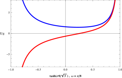
As already visible from Figure 1, in our setup a dyonic AdS${}_{2}\times\mathbb{R}^{2}$ solution is also possible when $\sigma_{0}=0$, i.e. when the scalar is not sourced. In this case the conditions (3.1) become

$$\ell^{-2}=-V\,,\qquad E^{2}+B^{2}=-{\frac{V}{2}}\,,\qquad\tan 2\omega=\frac{B^{2}-E^{2}}{2EB}\,.$$ (3.6)

This is in sharp contrast with the truncation studied in [5], which can be obtained by setting $\omega=\pi/4$ in our setup. In that case $\sigma_{0}=0$ implied $EB=0$, i.e. having both electric and magnetic fields sourced the (pseudo) scalar field. This is no longer true in the presence of a generic $\omega$-deformation – the more complicated structure of the gauge kinetic functions (2.17) when $\omega\neq\pi/4$ allows for a solution with vanishing $\sigma$. As a result, the standard dyonic AdS RN black hole is a solutions to the $\omega$ deformed theories, provided the constraints (3.6) are met.

3.2 Lifshitz and hyperscaling violating solutions

Next, we would like to ask whether our model supports zero temperature (non-relativistic) hyperscaling violating solutions in the deep IR of the geometry, i.e. at leading order in $r$ as $r\rightarrow 0$. Using our metric parametrization (2.1.1), geometries which describe Lifshitz scaling and hyperscaling violation take the form

$$ds^{2}=-r^{\frac{2(\theta-2z)}{\theta-2}}dt^{2}+r^{\frac{4}{\theta-2}}dr^{2}+r^{2}\,d\vec{x}^{2}\,,$$ (3.8)

and are typically supported by a running dilatonic scalar. We consider purely magnetic solutions in which the charged scalar field is not present, and therefore take our ansatz (2.1.1) to be of the form

$$f(r) = f_{0}\,r^{p}\,,\quad\sigma(r)=\frac{1}{\sqrt{3}}\log\sigma_{0}+\kappa\log r\,,\quad\phi(r)=0\,,\quad\rho(t,r,x,y)=0\,,$$ (3.9)

where we have anticipated that we expect the scalar to run logarithmically in the hyperscaling violation background.

An appropriate combination of Einstein’s equations then takes the simple form

$$\sigma^{\prime\,2}+\frac{2\beta^{\prime}}{r}=\frac{\kappa^{2}}{r^{2}}+\frac{2\beta^{\prime}}{r}=0\,,$$ (3.10)

whose solution is

$$\beta(r)=-\frac{\kappa^{2}}{2}\log r+C_{1}\,,$$ (3.11)

where we are allowing for an arbitrary constant. Thus, it will be the parameters $\{\kappa,p\}$ which will determine the scaling exponents $\{z,\theta\}$ through the relations

$$\theta=2-\frac{4}{p}\,,\quad z=\frac{\theta}{2}-1+\frac{\kappa^{2}}{8}(2-\theta)\,.$$ (3.12)

By solving the remaining equations of motion for the system and ensuring that they are satisfied to leading order in $r$, we find that we are forced to set (assuming for now $\kappa>0$)

$$p=1\,,\quad\kappa=\sqrt{3}$$ (3.13)

together with

$$B^{2}=\frac{g^{2}\,\cos^{2}\omega}{6\,\sigma_{0}^{4/3}}\,,\qquad f_{0}=\frac{16g^{2}}{33\,\sigma_{0}^{1/3}}\,.$$ (3.14)

Note that (3.13) implies the following values for the scaling exponents,

$$z=\frac{3}{2}\,,\quad\theta=-2\,.$$ (3.15)

So far we have assumed that the scalar $\sigma$ was positive. There is another branch of solutions on which it is negative,

$$\sigma(r)=-\frac{1}{\sqrt{3}}\sigma_{0}-\kappa\log r\,,$$ (3.16)

with the same scaling exponents but with a rotated value for the magnetic field,

$$p=1\,,\quad\kappa=\sqrt{3}\,,\quad B^{2}=\frac{g^{2}\sin^{2}\omega}{6\sigma_{0}^{4/3}}\,,\quad f_{0}=\frac{16g^{2}}{33\sigma_{0}^{1/3}}\,.$$ (3.17)

The scaling exponents (3.15) are the same as the ones found in [13] for the SUGRA truncation studied in [5], which corresponds to taking $\omega=\frac{\pi}{4}$ and $g=2$. The main difference here is the $\omega$ dependence appearing in (3.14) and (3.17). Recall that in our model the couplings of the scalar $\sigma$ to the gauge field and the scalar potential depend on various combinations of exponentials of the form $e^{\pm\sqrt{3}\sigma}$ as well as $e^{\pm\frac{\sigma}{\sqrt{3}}}$, whose arguments do not depend on $\omega$. Since it is precisely the structure of the argument of the exponentials that fixes the scaling exponents, our construction unfortunately does not allow for $\omega$-dependent values for $\{z,\theta\}$.

4 Black hole solutions

We are now ready to study the behavior of dyonic black hole solutions in the $\omega$-deformed theories described by (2.18), for the case in which the neutral and charged complex scalars vanish, $x=\rho=\chi=0$. We are interested in geometries which are asymptotic to AdS₄, so that the dual gauge theory will be a CFT in $2+1$ dimensions. We also want the latter to be at finite density, with chemical potential $\mu$ and magnetic field $B$. We work with the background ansatz (2.1.1), which we include again here for convenience,

$$ds^{2} = -e^{-\beta(r)}f(r)dt^{2}+\frac{dr^{2}}{f(r)}+r^{2}d\vec{x}^{2}\,,$$

$$A = \phi(r)\,dt+{\textstyle{\frac{\scriptstyle 1}{\scriptstyle 2}}}B(xdy-ydx)\,,\qquad\sigma=\sigma(r)\,,$$ (4.1)

and we start constructing the solutions by writing down the expansions for the geometry about the boundary and the horizon.
UV expansion
At the boundary, as $r\rightarrow\infty$, the metric should approach AdS₄ and the system should be at finite density. We solve the equations of motion perturbatively in $1/r$ (setting $G=1/16\pi$) and find the following expansion,

$$f = g^{2}r^{2}+\frac{g^{2}\sigma_{1}^{2}}{4}-\frac{1}{2r}(\varepsilon-{\textstyle{\frac{\scriptstyle 4}{\scriptstyle 3}}}\sigma_{1}\sigma_{2})+\ldots,$$

$$\beta = \beta_{0}+\frac{\sigma_{1}^{2}}{4r^{2}}+\frac{2\sigma_{1}\sigma_{2}}{3r^{3}}+\ldots,$$

$$\phi = e^{-\beta_{0}/2}\Big{(}\mu-\frac{q}{r}-\frac{\sqrt{3}B\sigma_{1}\sin 2\omega-\sqrt{3}q\sigma_{1}\cos 2\omega}{2r^{2}}\Big{)}+\ldots,$$

$$\sigma = \frac{\sigma_{1}}{r}+\frac{\sigma_{2}}{r^{2}}+\frac{5\sigma_{1}^{3}}{72r^{3}}+\ldots\,.$$ (4.2)

The parameters $\sigma_{1}$ and $\sigma_{2}$ represent, respectively, the source and VEV of the operator $\mathcal{O}_{\sigma}$ dual to the scalar. In our numerics we will turn off the source $\sigma_{1}$ for $\mathcal{O}_{\sigma}$ and take its scaling dimension to be $\Delta=2$, corresponding to a relevant deformation of the UV CFT. Thus, taking into account the choice $\sigma_{1}=0$, we have six parameters describing the UV expansion of the geometry, $\{\varepsilon,\sigma_{2},\beta_{0},\mu,q,B\}$.

IR expansion
The near-horizon $r\sim r_{+}$ behavior of the background takes the form

$$f = f_{+}(r-r_{+})+\ldots,$$

$$\beta = \beta_{+}+\ldots,$$

$$\phi = \phi_{+}(r-r_{+})+\ldots,$$

$$\sigma = \sigma_{+}+.\ldots\,,$$ (4.3)

described by the four parameters $\{\beta_{+},\phi_{+},\sigma_{+},r_{+}\}$, with

$$f_{+}=3r_{+}g^{2}\cosh\frac{\sigma_{+}}{\sqrt{3}}-\frac{B^{2}+\phi_{+}^{2}r^{4}_{+}e^{\beta_{+}}}{r^{3}_{+}(\cosh\sqrt{3}\sigma_{+}-\cos 2\omega\sinh\sqrt{3}\sigma_{+})}.$$ (4.4)

The higher order terms in the IR expansion are somewhat involved and will therefore not be included here. The numerical analysis will take them into account.

Similarly to [13], the equations of motion for our dyonic black hole ansatz are invariant under the two scaling symmetries

$$t\rightarrow\lambda t,\quad e^{\beta}\rightarrow\lambda^{2}e^{\beta},\quad\phi\rightarrow\lambda^{-1}\phi\,;$$

$$r\rightarrow r,\quad(t,x,y)\rightarrow\lambda^{-1}(t,x,y),\quad f\rightarrow\lambda^{2}g,\quad\phi\rightarrow\lambda\phi,\quad B\rightarrow\lambda^{2}B.$$ (4.5)

After solving the full set of equations numerically by integrating out from the horizon to infinity, we will use the first scaling symmetry to fix $\beta_{0}=0$. We will use the second scaling symmetry to identify the scale-invariant quantities $T/\mu$, $B/\mu^{2}$ with which we will label inequivalent solutions.

4.1 Thermodynamics

Following the discussion of [5], we analytically continue by setting $t=-i\tau$, and $I=-iS$. We can then obtain two expressions for the on-shell action for the class of the solutions we are studying. The first expression is given by the integral of a total derivative

$$I_{\rm bulk}=\frac{\Delta\tau{\rm vol}_{2}}{16\pi G}\int_{r_{+}}^{\infty}dr[r^{2}e^{-\beta/2}(f^{\prime}-f\beta^{\prime}-4U(\sigma)e^{\beta}\phi\phi^{\prime})+4BW(\sigma)\phi]^{\prime},$$ (4.6)

where ${\rm vol}_{2}\equiv\int dx^{1}dx^{2}$. The second can be written as

$$I_{\rm bulk}=\frac{\Delta\tau{\rm vol}_{2}}{16\pi G}\int_{r_{+}}^{\infty}dr\{[2rfe^{-\beta/2}]^{\prime}+4B^{2}r^{-2}e^{-\beta/2}U(\sigma)+4BW(\sigma)\phi^{\prime}\}.$$ (4.7)

The total action includes the Gibbons-Hawking surface term supplemented by counterterms

$$I_{\rm tot}=I_{\rm bulk}+I_{\rm surf}+I_{\rm ct},$$ (4.8)

where

$$I_{\rm surf} = \frac{1}{8\pi G}\int_{\partial{\cal M}}d\tau d^{2}x\sqrt{h}K\,,$$

$$I_{\rm ct} = \frac{1}{8\pi G}\int_{\partial{\cal M}}d\tau d^{2}x\sqrt{h}\Big{(}\frac{2}{\ell}+\frac{\ell}{2}{\cal R}\Big{)}+\frac{1}{48\pi G}\int_{\partial{\cal M}}d^{3}x\sqrt{h}\Big{(}\sigma n^{\mu}\partial_{\mu}\sigma-\frac{1}{2\ell}\sigma^{2}\Big{)}\,.$$ (4.9)

In the equation above $K_{\mu\nu}\equiv-{\textstyle{\frac{\scriptstyle 1}{\scriptstyle 2}}}(\nabla_{\mu}n_{\nu}+\nabla_{\nu}n_{\mu})$ is the extrinsic curvature of the boundary surface, with $n_{\mu}$ being the outward unit normal vector. The curvature radius of AdS is $\ell=1/g$, and ${\cal R}$ is the Ricci scalar of the boundary metric. It should be mentioned that here we use the counterterms given in [29], which are different from the ones used in [13]. The reason is that the counterterms chosen by [13] apply specifically to the cases where the scalar $\sigma$ satisfies Dirichlet or Neumann boundary conditions, corresponding to $\sigma_{1}=0$ or $\sigma_{2}=0$. However, from the dyonic black holes found in [29], one can see that the system studied here also admits black hole solutions in which $\sigma$ satisfies the mixed boundary condition $\sigma_{2}\propto\sigma_{1}^{2}$ corresponding to turning on a triple trace deformation in the dual theory. It was shown in [31] that the boundary condition $\sigma_{2}\propto\sigma_{1}^{2}$ preserves all the asymptotic AdS symmetries, therefore the holographic stress tensor should be traceless in this case. As we show below, while the stress tensor calculated using the boundary term [29] has such a property.

Using these counterterms, the renormalized energy-momentum tensor is given by $T^{\mu\nu}\equiv(2/\sqrt{-h})\,\delta I/\delta h_{\mu\nu}$, yielding

$$T_{\mu\nu}=\frac{1}{8\pi G}\Big{(}K_{\mu\nu}-Kh_{\mu\nu}-\frac{2}{\ell}h_{\mu\nu}+\ell\,({\cal R}_{\mu\nu}-{\textstyle{\frac{\scriptstyle 1}{\scriptstyle 2}}}{\cal R}\,h_{\mu\nu})+\frac{1}{6}h_{\mu\nu}(\sigma n^{\rho}\partial_{\rho}\sigma-\frac{1}{2\ell}\sigma^{2})\Big{)}\,.$$ (4.10)

The stress tensor $\tau^{i}_{~{}j}$ of the dual boundary theory can be calculated as

$$\tau^{i}_{~{}j}=2r^{3}T^{i}_{~{}j}|_{r=\infty},$$ (4.11)

from which we find

$$\tau^{t}_{~{}t}=-\varepsilon,\quad\tau^{x}_{~{}x}=\tau^{y}_{~{}y}=\frac{\varepsilon}{2}.$$ (4.12)

We notice that the energy density coincides with the AMD mass density [32], and the stress tensor of the dual CFT is traceless as expected.

Next, we define the thermodynamic potential $W\equiv T[I_{\rm tot}]\equiv{\rm vol}_{2}w$, where the temperature of the black hole is given by

$$T=\frac{e^{(\beta_{0}-\beta_{+})/2}f_{+}}{4\pi}.$$ (4.13)

Using the expression (4.6) and the expansions (4.2) and (4.3), we obtain

$$w=\varepsilon-4\mu q-Ts\,,$$ (4.14)

where the $s$ is the entropy density given by

$$s=4\pi r^{2}_{+}\,.$$ (4.15)

On the other hand, making use of (4.7), we obtain

$$w=-\frac{\varepsilon}{2}+4e^{\beta_{0}/2}\int_{r_{+}}^{\infty}dr\{B^{2}r^{-2}e^{-\beta/2}U(\sigma)+BW(\sigma)\phi^{\prime}\}.$$ (4.16)

Equating this expression with (4.14) would give a Smarr type formula. Following the Wald procedure, the first law of thermodynamics takes the form

$$\delta\varepsilon=T\delta s+4\mu\delta q-m\delta B+{\textstyle{\frac{\scriptstyle 1}{\scriptstyle 3}}}g^{2}(\sigma_{1}\delta\sigma_{2}-2\sigma_{2}\delta\sigma_{1}),$$ (4.17)

where $m$ is the magnetization per unit volume

$$m=-4e^{\beta_{0}/2}\int_{r_{+}}^{\infty}dr\{Br^{-2}e^{-\beta/2}U(\sigma)+W(\sigma)\phi^{\prime}\}.$$ (4.18)

Finally, using the formulae given in Appendix A, we would like to show how the free energy of the $\omega$-deformed theory differs from that of the undeformed theory. Recall that the $U(1)$ field strength in the $\omega$-deformed theory is related to the undeformed one by a duality rotation,

$$F_{\omega}=\cos\omega F_{0}-\sin\omega e^{\sqrt{3}\sigma}*F_{0}\,.$$ (4.19)

Plugging in the dyonic black hole ansätz for $F$,

$$F=-\phi^{\prime}dt\wedge dr+Bdx\wedge dy\,,$$ (4.20)

we obtain

$$\phi^{\prime}_{\omega}=\cos\omega\phi^{\prime}_{0}+\sin\omega e^{\sqrt{3}\sigma}e^{-\beta/2}B_{0}/r^{2},\quad B_{\omega}=\cos\omega B_{0}-r^{2}e^{\beta/2}e^{\sqrt{3}\sigma}\sin\omega\phi^{\prime}_{0}\,.$$ (4.21)

Using the UV expansion of the fields (4.2), we can derive

$$q_{\omega}=\cos\omega q_{0}+\sin\omega B_{0},\quad B_{\omega}=\cos\omega B_{0}-\sin\omega q_{0},\quad\mu_{\omega}=\cos\omega\mu_{0}-{\textstyle{\frac{\scriptstyle 1}{\scriptstyle 4}}}\sin\omega m_{0}.$$ (4.22)

Under the duality rotation the energy, temperature and entropy of the black hole solutions do not change, but the free energy does, so that

$$w_{\omega}=\varepsilon-4\mu_{\omega}q_{\omega}-Ts\;\;\neq\;\;w_{0}=\varepsilon-4\mu_{0}q_{0}-Ts\,.$$ (4.23)

4.2 Magnetic Field Induced Transitions

We have constructed dyonic black hole solutions to our $\omega$-deformed theories numerically by building on the UV and IR expansions (4.2) and (4.3). The solutions have AdS₄ asymptotics, to ensure that in the UV the dual theory is described by a three-dimensional CFT. Moreover, we have taken the source $\sigma_{1}$ for the operator $\mathcal{O}_{\sigma}$ dual to $\sigma$ to be zero – to avoid deforming the UV CFT – and chosen its conformal dimension to be $\Delta=2$, corresponding to a relevant perturbation. We expect to find a rich phase structure as one varies the magnetic field and temperature in the system. In particular, from the analysis of [13] (corresponding to the deformation choice $\omega=\pi/4$) we expect to find a line of first order metamagnetic transitions when the magnetic field becomes sufficiently large. Indeed, this will be a generic feature of our $\omega$-deformed theories. Moreover, as we cool the thermodynamically preferred black holes down to zero temperature, the resulting domain-wall solutions will approach either AdS${}_{2}\times\mathbb{R}^{2}$ or a hyperscaling violating solution in the IR, depending on the strength of $B$. To facilitate the comparison with [13], we will adopt their notation from here on.

Let’s start by discussing how the temperature dependence of the free energy is affected by the magnetic field. In Figure 2 we show a typical plot of the free energy as a function of temperature for a moderately low value of $B$, which we take to be in the range

$$0<\frac{B}{\mu^{2}}<\left(\frac{B}{\mu^{2}}\right)_{I}\,,$$ (4.24)

with $\left(B/\mu^{2}\right)_{I}$ to be defined shortly.

Figure 2: Typical plot of the free energy as a function of temperature for $\omega=\pi/8$ and $g=2$ when the magnetic field is in the range (4.24). The solid lines describe black holes whose zero temperature limits are domain-walls approaching in the IR AdS${}_{2}\times\mathbb{R}^{2}$ (denoted by dots). The thick dashed line describes black holes whose domain-wall limit approach hyperscaling violating solutions in the IR. The thin dashed line is a naive extrapolation of the numerical data (thick dashed line) to very low temperatures.

We have chosen $\omega=\pi/8$, but the structure seen in the figure is insensitive to the specific value of the $\omega$ parameter. We find three branches of solutions, only one of which can seemingly be heated up to arbitrarily high temperatures. The solid lines describe black hole geometries whose zero temperature limit are domain-walls approaching dyonic AdS${}_{2}\times\mathbb{R}^{2}$ solutions in the IR. The latter belong to the electric family we described in Section 3 and are denoted by dots in the plot. On the other hand, the (thick) dashed line describes a black hole whose zero temperature, deep IR limit is a hyperscaling violating solution of the type discussed in Section 3.2. In all the figures in this section the thin dashed lines are a naive extrapolation of the numerics (thick dashed lines) to very low temperatures.

We see from the figure that there are two distinct dyonic AdS${}_{2}\times\mathbb{R}^{2}$ geometries at $T=0$ (denoted by the two dots). The black hole branch which is thermodynamically preferred is the one whose temperature can be arbitrarily high, and approaches the AdS${}_{2}\times\mathbb{R}^{2}$ with the lower free energy. The phase structure shown in Figure 2 turns out to be typical as long as the magnetic field is in the range (4.24). In this discussion we will assume that $B>0$ but the same argument goes through for a negative field. The value $\frac{B}{\mu^{2}}=\left(\frac{B}{\mu^{2}}\right)_{I}$ (which is $\omega$-dependent) is defined to be such that, at zero temperature, the bottom AdS${}_{2}\times\mathbb{R}^{2}$ solution overlaps with the hyperscaling violating one – the two geometries have the same free energy. Thus, if the magnetic field is any larger, at very low temperatures the hyperscaling violating branch becomes thermodynamically preferred. The temperature dependence of the magnetization $m$ when the field is within the range (4.24) is shown by the red curve in Figure 4. In the left panel the thermodynamically preferred black hole branch corresponds to the bottom (red) curve, along which $B>0$ and $m$ becomes more negative as the temperature is raised. Thus, the system is becoming more ordered as it is heated, with the magnetization opposing the direction of the magnetic field. On the other hand in the right panel it is the top (red) curve which is favored, along which both $B$ and $m$ are negative, and the latter becomes less negative as $T$ increases. In this case the magnetization is aligned with the field, and the system becomes less ordered as the temperature is raised.

As $B/\mu^{2}$ is raised above $\left(B/\mu^{2}\right)_{I}$, the two zero temperature AdS${}_{2}\times\mathbb{R}^{2}$ solutions become closer to each other, and overlap when the ratio reaches a critical value which we denote by $\left(B/\mu^{2}\right)_{max}$. At this point there is only a single domain-wall solution whose IR is a dyonic AdS${}_{2}\times\mathbb{R}^{2}$ geometry belonging to the electric family. This behavior is visible in Figure 3, where we plot the free energy as a function of temperature for increasing values of magnetic field and for $\omega=\pi/8$. In the left panel we have taken $B>0$ and the field increases from bottom to top. On the other hand in the right panel $B<0$ and becomes more negative from top to bottom.

Figure 3: Free energy as a function of temperature for $\omega=\pi/8$ and $g=2$, for different values of $B/\mu^{2}$. In the left (right) panel the magnetic field is positive (negative), and $B$ increases (decreases) from bottom to top. The solid/dashed lines and the dots are the same as in Figure 2. The open circles mark the point at which the thermodynamically preferred branch switches from the one with AdS${}_{2}\times\mathbb{R}^{2}$ in the IR to the hyperscaling violating branch.

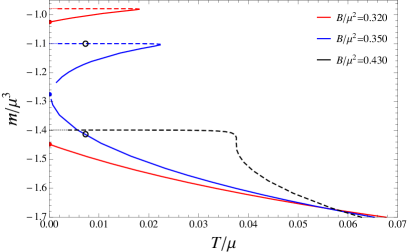
In Figure 3 the overlap of the two $T=0$ AdS${}_{2}\times\mathbb{R}^{2}$ geometries occurs for the choice of magnetic field shown in the blue curve, i.e. $\left(B/\mu^{2}\right)_{max}=0.350$ in the left panel and $\left(B/\mu^{2}\right)_{max}^{neg}=-0.163$ in the right panel. Thus, when the field is such that

$$\left(\frac{B}{\mu^{2}}\right)_{I}<\frac{B}{\mu^{2}}\leq\left(\frac{B}{\mu^{2}}\right)_{max}\,,$$ (4.25)

the branch which is thermodynamically favored at low temperatures is the hyperscaling violating one. As the temperature is raised, we eventually cross over to the black hole branch with an associated $T=0$ AdS${}_{2}\times\mathbb{R}^{2}$ IR description, which dominates at sufficiently high temperatures. We emphasize that this behavior is typical when the magnetic field is within the range (4.25).

The transition between the two branches is first order, as visible from the cusp in the free energy plot where the two lines meet. This is also confirmed by the behavior of the magnetization, displayed in Figure 4. As we move from one black hole branch to the other by following the blue curve in the figure, the magnetization suffers a sudden, discontinuous jump, i.e. it undergoes a metamagnetic first order phase transition. This was already seen in [13] for the particular $\omega=\pi/4$ case, and is generic in our $\omega$-deformed theories.

Figure 4: Magnetization as a function of temperature for $\omega=\pi/8$ and $g=2$, for different values of $B/\mu^{2}$. In the left (right) panel the magnetic field is positive (negative). The solid/dashed lines and the dots are the same as in Figure 2. The open circles mark the point at which the magnetization undergoes a sudden jump, denoting a first order metamagnetic phase transition.

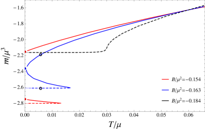
Metamagnetic transitions occur in a number of materials [25, 26], including strongly correlated electrons systems. An example is the layered ruthenate metal $Sr_{3}Ru_{2}O_{7}$, which exhibits – for a sufficiently large value of magnetic field – a line of first order, non-zero temperature metamagnetic phase transitions which end at a critical point. In the particular $Sr_{3}Ru_{2}O_{7}$ compound the critical point can become quantum critical by appropriately tuning the magnetic field [27] (for a related holographic study see [11]). Another interesting feature we notice from Figure 4 is that in all the curves with $B/\mu^{2}>\left(B/\mu^{2}\right)_{I}$ the magnetization saturates to a nearly constant value at low temperatures. We emphasize that the saturation lines correspond to the cases for which the dominant $T=0$ geometry is hyperscaling violating. Such low-temperature plateaus also occur in systems which exhibit metamagnetic phase transitions (see e.g. [28]). It would be interesting to make the connection to real metamagnetic materials more concrete.

When the magnetic field becomes larger than $B_{max}$, the domain walls with AdS${}_{2}\times\mathbb{R}^{2}$ in the deep IR cease to exist, and the only black hole branch which can be cooled down to zero temperature always exhibits hyperscaling violation in the IR. The magnetization suffers a discontinuous jump until we reach a critical value of the magnetic field, $B_{c}>B_{max}$ at which we find only one black hole solution and the magnetization starts changing in a continuous matter. Thus, the line of first order phase transitions stops at a critical point, where the phase transition becomes continuous. This is visible in the black line shown in Figure 4, which corresponds to the critical point $B=B_{c}$ and therefore to the black hole branch exhibiting hyperscaling violation at $T=0$. Following the behavior of $m$ along the black line as the temperature increases, we note that there is a critical temperature at which the derivative of $m/\mu$ with respect to $T/\mu$ is infinite, i.e. the phase transition is second order (or higher). Finally, when $B>B_{c}$ we no longer have a phase transition as we vary $T/\mu$. Before we conclude this discussion we would like to point out that, unlike in the special case $\omega=\pi/4$, the curves we have displayed are not anti-symmetric as $B\rightarrow-B$ (remember that when $\omega=\pi/4$ (2.32) and (2.32) combine to become a symmetry).

To summarize the results of this section, we have seen three distinct regimes, depending on the strength of the magnetic field:

1. For $0<\frac{B}{\mu^{2}}\leq\left(\frac{B}{\mu^{2}}\right)_{I}$ the thermodynamically preferred black holes can always be cooled down to domain-wall solutions with a dyonic AdS${}_{2}\times\mathbb{R}^{2}$ geometry in the IR. The magnetization associated with such black holes changes smoothly and monotonically as a function of temperature.

2. When $\left(\frac{B}{\mu^{2}}\right)_{I}<\frac{B}{\mu^{2}}\leq\left(\frac{B}{\mu^{2}}\right)_{max}$ the black holes favored at low temperatures approach a hyperscaling violating solution in the IR, as they are cooled to $T=0$. On the other hand the black holes which are favored at higher temperatures are those whose domain-walls have an AdS${}_{2}\times\mathbb{R}^{2}$ IR description. The latter domain-wall solutions no longer exist when $\frac{B}{\mu^{2}}>\left(\frac{B}{\mu^{2}}\right)_{max}$. The magnetization undergoes a first order metamagnetic phase transition as a function of temperature when $\left(\frac{B}{\mu^{2}}\right)_{I}<\frac{B}{\mu^{2}}<\left(\frac{B}{\mu^{2}}\right)_{c}$, where the ratio $\left(\frac{B}{\mu^{2}}\right)_{c}>\left(\frac{B}{\mu^{2}}\right)_{max}$ denotes the value at which the transition becomes continuous.

3. Above $\left(\frac{B}{\mu^{2}}\right)_{c}$ there is only one black hole branch, whose $T\rightarrow 0$ limit approaches a hyperscaling violating solution in the IR. The magnetization no longer undergoes a phase transition as we vary the temperature of the system.

The behavior we have discussed is generic, independently of the of the $\omega$-deformation parameter, and its main features agree with the $\omega=\pi/4$ case studied in [5].

5 Domain wall solutions

The zero-temperature description of the black holes we constructed in Section 4 should be domain-wall geometries with AdS₄ asymptotics, approaching either dyonic AdS${}_{2}\times\mathbb{R}^{2}$ solutions or hyperscaling violating geometries in the IR, depending on the value of the magnetic field. In this section we will focus on the former case, and construct numerically domain-walls with an IR AdS${}_{2}\times\mathbb{R}^{2}$ description by cooling down the corresponding black holes to very low temperatures. Our main goal here is to discuss briefly the phase space of the solutions, and the dependence of the free energy and magnetization on the magnetic field $B$ in the system. We are particularly interested in features that may be entirely due to the $\omega$-deformation.

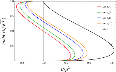
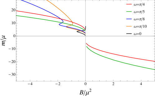
We start by discussing solutions which belong to the electric family we introduced in Section 3, displayed in Figures 5 and 6. The left panel of Figure 5 shows the magnetic field dependence of the IR value $\sigma_{0}$ of the scalar field, for several choices of $\omega$-deformation. The red (left-most) line corresponds to the $\omega=\pi/4$ case studied in [13], and is symmetric under (2.34). As the deformation parameter $\omega$ is lowered towards $\omega=0$ the solutions shift to the right and the symmetry (2.34) is lost. The dots denote the appearance of tachyonic fluctuations which violate the BF bound for AdS₂ and are responsible for triggering superfluid instabilities, as we will see in detail in Section 6.

Figure 5: Domain-wall solutions belonging to the electric family for various choices of $\omega$. Left panel: dependence of the horizon value of the scalar on the magnetic field. The dots denote the appearance of tachyonic modes which violate the AdS₂ BF found. Right panel: free energy as a function of magnetic field. The branches that are thermodynamically preferred are the ones which extend to $B=0$.

Figure 6: Magnetic field dependence of the magnetization for the electric family of solutions, for different choices of $\omega$. Left panel: when $B>0$ on the thermodynamically preferred branches we have $m>0$ when $\omega=\pi/4$, and $m<0$ for the other choices of $\omega$-deformations. Right panel: the $\omega$-deformation is chosen so that the magnetization changes sign on the thermodynamically preferred branch when $B>0$.

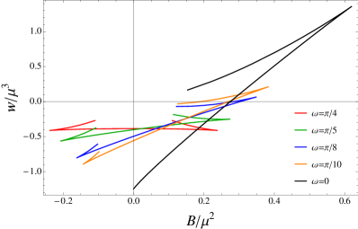
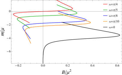
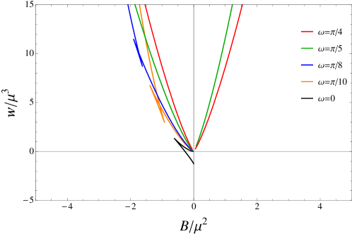
The right panel of Figure 5 shows the dependence of the free energy on the magnetic field for each family of solutions. Each line (corresponding to a distinct value of $\omega$) has two branches, with the thermodynamically favored one extending all the way to $B=0$ for each choice of deformation parameter. It is visible from this figure that the symmetry between positive and negative values of the magnetic field is lost once we move away from the special deformation $\omega=\pi/4$.

Finally, Figure 6 displays the behavior of the magnetization as the magnetic field changes, for each family of solutions. Let us discuss the left panel first, and for simplicity restrict our attention to the $B>0$ sector. The red (top) line is the $\omega=\pi/4$ case, for which the magnetization is always positive and aligned with the magnetic field, hence the system displays paramagnetism. In the remaining lines we find $m<0$ on the thermodynamically preferred branches, i.e. the magnetization opposes the magnetic field and the system is diamagnetic. Moreover, notice that for all the cases for which $\omega\neq\pi/4$, we see a residual magnetization at zero magnetic field.

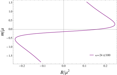
Interestingly, for certain values of the deformation parameter it is possible to find thermodynamically preferred branches on which the magnetization can change sign, even though $B$ does not. This is shown in the right panel of Figure 6 for the specific choice $\omega=24\pi/100$. There $m$ changes sign, starting out positive at the maximum value of $B$ and becoming smaller and eventually negative as $B$ decreases towards zero. Thus, the system is paramagnetic for large values of the magnetic field, and becomes diamagnetic as $B$ is tuned to smaller values. We emphasize that this behavior is not possible in the $\omega=\pi/4$ truncation. Here we also see a residual magnetization when $B=0$.

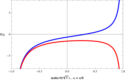
We now switch to discussing the domain-wall solutions which belong to the magnetic family, which we display in Figures 7, 8 and 9. We would like to revisit the expectation from [13] that solutions in the electric family would always be thermodynamically preferred, compared to those in the magnetic family. We will provide some argument supporting this expectation, even in the case of general $\omega$-deformations. As before, we have constructed the domain-wall solutions numerically by cooling the black holes of Section 4 to low temperatures, reaching $T/\mu\sim 10^{-5}$.

Figure 7: Domain wall solutions belonging to the magnetic family, for different values of $\omega$ and for $g=2$.

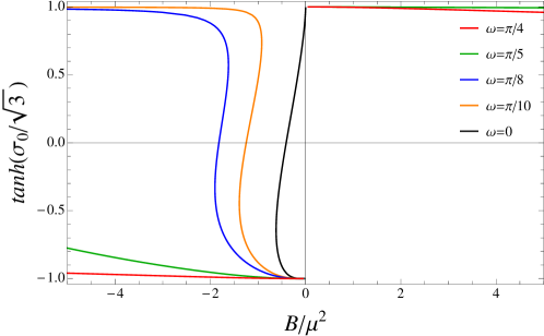
Figure 7 displays the dependence of $\sigma_{0}$ on the magnetic field. We find that when $\tanh(\sigma_{0}/\sqrt{3})$ is very close to one it is difficult to construct the solutions numerically. Thus, we were not able to obtain the $\omega=\pi/8,\pi/10$ branches which should appear in the first quadrant. Finally, Figures 8 and 9 show, respectively, the free energy and magnetization as a function of magnetic field. We were able to probe only a small region where both electric and magnetic families coexist. In this region, the domain-walls in the electric family are always thermodynamically preferred. Moreover, as we heat up the solutions, the free energy of the black holes coming from the magnetic (electric) family increases (decreases). This provides further evidence which indicates that the electric branch is always thermodynamically favored. Clearly it would be valuable to confirm this with further studies.

Figure 8: Free energy of the domain-wall solutions belonging to the magnetic family, for different values of $\omega$ $g=2$.

Figure 9: Magnetization as a function of magnetic field for the the domain-wall solutions belonging to the magnetic family, for different values of $\omega$ $g=2$.

6 Superfluid instability

So far we have restricted our attention to solutions for which the charged complex scalar field vanishes, $\rho\,e^{i\chi}=0$. However, when the background geometry is described by black holes whose extremal limit has a near-horizon AdS${}_{2}\times\mathbb{R}^{2}$, we expect the field to condense at some critical temperature $T_{c}$, spontaneously breaking the $U(1)$ and triggering a superfluid phase transition [14, 15, 16]. In this section we will examine the appearance of such superfluid instabilities in the dyonic black hole backgrounds we constructed in Section 4, when the magnetic field is in the range (4.24). However, the presence of unstable modes can already be anticipated by considering linearized fluctuations $\delta\rho$ of the charged scalar about the AdS${}_{2}\times\mathbb{R}^{2}$ solutions of Section 3, for which $\rho=0$. The system will be unstable when there are tachyonic modes which violate the BF bound for AdS₂. To see this more explicitly, we examine the equation of motion for the scalar perturbation $\delta\rho$ on this background, which takes the form

$$\square\delta\rho-4g^{2}A^{2}\,\delta\rho-{\frac{{\partial}^{2}V}{{\partial}\rho^{2}}}\,\delta\rho=0\,,$$ (6.1)

and hence

$$\square\delta\rho=g^{2}\left[B^{2}(x_{1}^{2}+x_{2}^{2})-4\ell^{2}E^{2}+\left(\cosh(\sqrt{3}\sigma_{0})-3\cosh{\frac{\sigma_{0}}{\sqrt{3}}}+4\cos 2\omega\,\sinh^{3}{\frac{\sigma_{0}}{\sqrt{3}}}\right)\right]\delta\rho\,.$$

We take the fluctuation to describe the first Landau level, which we expect to condense first [16],

$$\delta\rho=u(t,r)\,e^{-{\textstyle{\frac{\scriptstyle 1}{\scriptstyle 2}}}g|B|(x_{1}^{2}+x_{2}^{2})}\,.$$ (6.2)

It then follows that

$$\square_{AdS_{2}}\,u=M^{2}\,u\,,$$ (6.3)

where $\square_{AdS_{2}}$ is the d’Alembertian on the AdS₂ spacetime and

$$M^{2}=2g\,|B|-4g^{2}\ell^{2}\,E^{2}-3g^{2}\cosh{\frac{\sigma_{0}}{\sqrt{3}}}+g^{2}\cosh(\sqrt{3}\sigma_{0})+4g^{2}\cos 2\omega\,\sinh^{3}{\frac{\sigma_{0}}{\sqrt{3}}}\,.$$ (6.4)

Superfluid instabilities are triggered when the mass of the fluctuation becomes smaller than the BF bound for AdS₂, i.e. when $M^{2}<m_{BF}^{2}=-g^{2}/4$, which in our case is

$$\boxed{2g\,|B|-4g^{2}\ell^{2}\,E^{2}-3g^{2}\cosh{\frac{\sigma_{0}}{\sqrt{3}}}+g^{2}\cosh(\sqrt{3}\sigma_{0})+4g^{2}\cos 2\omega\,\sinh^{3}{\frac{\sigma_{0}}{\sqrt{3}}}<-\frac{g^{2}}{4}\,.\;}$$ (6.5)

Notice that stronger (weaker) electric (magnetic) fields enhance the instability window.

Figure 10: Dependence of $M^{2}/g^{2}+1/4$ on $\tanh(\sigma_{0}/\sqrt{3})$ for the domain-wall solutions shown in Figure 5, for different values of the $\omega$-deformation and with $g=2$. When the curves cross zero and become negative, the mass of the charged scalar fluctuation violates the AdS₂ BF bound, causing the zero temperature domain-wall to be unstable. The dots denote the point at which the instability sets in.

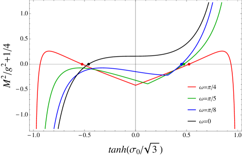
In Figure 10 we show the mass of the fluctuation $\delta\rho$ (more precisely, the shifted mass $M^{2}/g^{2}+1/4$) in the AdS${}_{2}\times\mathbb{R}^{2}$ background as a function of the IR value $\sigma_{0}$ of the scalar, as given in (6.5). Different curves corresponds to different choices of $\omega$-deformation. Superfluid instabilities are expected when each curve becomes negative, corresponding to the fluctuation violating the BF bound for AdS₂. The onset of the instability is denoted by a dot in the figure, and occurs when a line crosses the horizontal axis. Inspecting Figures 5 and 10, we note that when $\tanh(\sigma_{0}/\sqrt{3})<0$ (which corresponds to $B/\mu^{2}>0$) the BF bound is always violated for the curves with $\omega=\pi/5,\pi/8,\pi/10$. We will return to this point shortly.

What we are really interested in, however, are superfluid instabilities appearing in the dyonic black holes we studied in Section 4, with an IR AdS${}_{2}\times\mathbb{R}^{2}$ zero temperature description. Recall that the latter are always thermodynamically preferred when the field is relatively low, and in the range (4.24). Thus, our instability analysis will only describe the regime $B/\mu^{2}\leq\left(B/\mu^{2}\right)_{I}$. To determine whether the charged scalar field can condense at non-zero temperature, we will ask whether a normalizable mode of $\rho$ appears at some critical temperature denoted by $T_{c}$, for an appropriate range of magnetic field. Since we are interested in breaking the abelian gauge symmetry spontaneously, we do not want to generate a non-normalizable mode for $\rho$, corresponding to a source for the dual operator $\cal{O}_{\rho}$. To this end, we want to solve for the linearized fluctuation $\delta\rho$ assuming a background of the form of (2.1.1). We take the fluctuation to be of the form

$$\delta\rho=R(r)\,e^{-{\textstyle{\frac{\scriptstyle 1}{\scriptstyle 2}}}g|B|(x_{1}^{2}+x_{2}^{2})}\,.$$ (6.6)

Substituting it into the equation of motion for $\rho$ and working to linear order, we find

$$r^{-2}e^{\frac{\beta(r)}{2}}\left(r^{2}f(r)e^{-\frac{\beta(r)}{2}}R^{\prime}(r)\right)^{\prime}-\left(\frac{2g\left|B\right|}{r^{2}}+G(\sigma)-\frac{4g^{2}e^{\beta(r)}\phi(r)^{2}}{f(r)}\right)R(r)=0\\$$ (6.7)

where

$$G(\sigma)=g^{2}\left(-4\cos(2\omega)\sinh^{3}\left(\frac{\sigma(r)}{\sqrt{3}}\right)-3\cosh\left(\frac{\sigma(r)}{\sqrt{3}}\right)+\cosh\left(\sqrt{3}\sigma(r)\right)\right).$$

At the horizon, the radial perturbation $R(r)$ has an expansion of the form

$$R(r)=c_{1}+c_{2}\log(r-r_{+})+\ldots\;.$$ (6.8)

We set $c_{2}=0$ to ensure that $R(r)$ is regular . On the other hand, the boundary behavior of $R(r)$ is given by

$$R(r)=\frac{R_{1}}{r}+\frac{R_{2}}{r^{2}}\,,$$ (6.9)

with $R_{1}$ and $R_{2}$ denoting, respectively, the source and the VEV of the operator dual to the charged scalar.

By varying $T/\mu$, we find a solution for the $\delta\rho$ perturbation which has $R_{1}=0$ and $R_{2}\neq 0$, indicating that the field indeed condenses and the symmetry breaking is spontaneous, as desired.

Figure 11: Critical temperature at which the superfluid phase transition sets in, for different choices of $\omega$ and for $g=2$. The $\omega$ parameter for each curve decreases from top to bottom. The dots on the horizontal axis denote the points at which the mass of the charged scalar field fluctuation about the $T=0$ AdS${}_{2}\times\mathbb{R}^{2}$ IR geometry violates the AdS₂ BF bound, as shown in Figure 10.

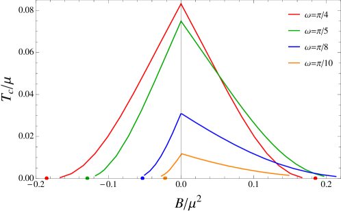
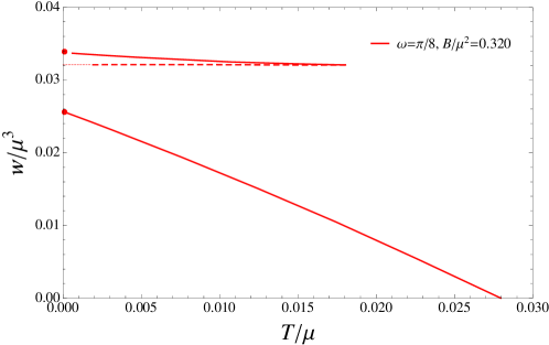
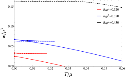
Our results are shown in Figure 11, where we plot the critical temperature $T_{c}$ at which the field starts to condense as a function of the external magnetic field, for different choices of $\omega$. We would like to highlight a few features of this analysis. First, as $T_{c}\rightarrow 0$ we expect the curves to approach the dots denoting superfluid instabilities of the zero temperature AdS${}_{2}\times\mathbb{R}^{2}$ geometry. Notice that there is a slight deviation between the dots and the low-$T_{c}$ regime of some of the curves. We expect this discrepancy to be a reflection of the fact that we are working in a linearized approximation, and that a fully back-reacted analysis would resolve it. In fact, recall that in [16], taking into account back-reaction lead to a suppression of $T_{c}$ compared to the probe limit result. The disagreement between the two cases became more important as $T_{c}\rightarrow 0$, i.e. away from the regime of validity of the probe approximation.

An interesting feature is that as we move $\omega$ away from $\pi/4$ while keeping $|B|$ very small, $T_{c}$ is suppressed (the suppression is not always present in the regime where the magnetic field is large). Thus, as $\omega$ decreases one has to reach lower temperatures in order to access the superfluid phase. We expect this to be especially a factor for the $\omega=0$ case, for which we were not able to reach $T_{c}$ in our numerics.

When $B<0$, we can easily see from Figure 11 that there is a range of magnetic field for which a condensate does not form. In particular, if the magnitude of the field is too large, it will prevent the formation of a superfluid phase, consistent with expectations from the Meissner effect. On the other hand, when $B>0$ as we decrease $\omega$ (moving from top to bottom in the figure) the range of $B$ which allows for a superfluid instability is seemingly becoming larger. In fact, the curves seem to flatten out as $B/\mu^{2}$ increases. This is consistent with the structure of Figure 10, where we saw that the blue and green curves always violated the AdS₂ BF bound for $B>0$. Thus, the superconducting phase naively seems to survive even in very strong magnetic fields. However, we should keep in mind that our instability analysis assumes that the magnetic field is in the range (4.24), and breaks down when $B/\mu^{2}=\left(B/\mu^{2}\right)_{I}$, at which point the thermodynamically preferred background is hyperscaling violating. Let’s return briefly to the behavior of the $\omega=0$ curve. By combining Figures 5 and 10 we see that, when $\omega$ is nearly zero, the value of $B$ for which the fluctuation $\delta\rho$ is tachyonic is already very close to $B_{max}$. Thus, there is a very narrow window in which the superfluid instability can occur. Moreover, this corresponds to a very low $T_{c}$, making it even harder to observe numerically.

6.1 Competition with stripe instabilities

As we already stressed in the introduction, AdS${}_{2}\times\mathbb{R}^{2}$ solutions are also known to be unstable to the formation of spatially modulated phases, triggered by modes which violate the AdS₂ BF bound and break translational symmetry (see the analysis of [13] for the dyonic case). Thus, we expect the domain-walls we constructed in Section 5 – which have an AdS₂ factor in their IR description – to also suffer from striped instabilities. By the same token, there should be spatially modulated tachyonic modes in the non-zero temperature generalizations of these solutions – the dyonic black holes of Section 4 – provided the magnetic field is in the range (4.24).

The authors of [13] discussed the competition between superfluid and spatially modulated instabilities in the context of the $\omega=\pi/4$ theory. In particular, for the class of dyonic AdS${}_{2}\times\mathbb{R}^{2}$ solutions to the theory they found that the existence of striped instabilities was independent of the value of the magnetic field. As a result, increasing the magnetic field should act to suppress the superfluid instabilities compared to the striped ones. In particular, a priori at non-zero temperature one expects both types of instabilities to be generically present as long as the field is in the range $0<|B|<|B^{SC}_{c}|<|B_{I}|$, where $B^{SC}_{c}$ denotes the point at which the charged scalar no longer condenses (i.e. the critical temperature for the superfluid phase transition becomes $T_{c}=0$). On the other hand, when $|B^{SC}_{c}|<|B|<|B_{I}|$ the superfluid phase is no longer accessible and only striped instabilities should survive.

For the $\omega$-deformed case the analysis of spatially modulated perturbations of the dyonic AdS${}_{2}\times\mathbb{R}^{2}$ solutions is analogous to that of [13]. In particular, the spectrum of the scaling dimensions for the fluctuations is the same, since a duality rotation relates the solutions of the $\omega$-deformed theory to those of [13], when the charged scalar field is turned off. The main difference in the $\omega$-deformed case comes from the behavior at non-zero temperature, and is due to the fact that the theory is no longer invariant under $B\rightarrow-B$. In particular, recall from Figure 11 that when $B>0$ the charged scalar naively appears to condense for arbitrarily high values of $B$, in contrast with expectations from the Meissner effect. However, since the instability analysis is only valid up to $B=B_{I}$, the latter value sets a natural cutoff for the existence of a superfluid phase. Still, for the $\omega$-deformed theories we expect to have both stripe and superfluid phases in the entire range $0<B<B_{I}$, unlike for the $\omega=\pi/4$ theory. On the other hand the behavior when $B<0$ is analogous to that of [13], with both instabilities present when $-|B^{S.C.}_{c}|<B<0$ and striped ones alone in $-|B_{I}|<B<-|B^{S.C.}_{c}|$.

It would be useful to determine the temperature at which the spatially modulated instabilities are triggered, and in particular whether it is above or below the one associated with the onset of the superfluid instability. Answering this question would be a first step towards better understanding the ultimate ground states of the $\omega$-deformed theories. Clearly, the question of back-reaction on the geometry is even more important, although challenging to investigate. We should also mention that the hyperscaling violating geometries themselves are believed to suffer, in certain cases, from striped instabilities. For discussions of this question we refer the reader to e.g. [33, 34, 35]. Thus, it is possible that we would find spatially modulated tachyonic modes even when the zero temperature geometry in the deep IR exhibits hyperscaling violation, for $|B|>|B_{I}|$.

7 Conclusions

The $\omega$-deformed supergravity truncations we have studied in this paper admit a rich variety of phases, which can be accessed by appropriately tuning the magnetic field of the system and varying its temperature. An interesting structure already emerges when we consider truncations which retain, in addition to a $U(1)$ gauge field, a single neutral scalar. Dyonic black hole solutions in this case exhibit a line of first order metamagnetic phase transitions – describing a sudden change in the magnetization – once $B$ is sufficiently strong. Moreover, as they are cooled down to zero temperature, they behave either as a diamagnetic or a paramagnetic material, depending again on the strength of $B$ and the particular choice of $\omega$. In these truncations the deep IR region of the extremal geometries is described by either dyonic AdS${}_{2}\times\mathbb{R}^{2}$ or a solution with a non-trivial dynamical critical exponent and hyperscaling violation. It is precisely the tension between black hole branches with these different IR descriptions which is responsible for the metamagnetic phase transition.

In less restrictive truncations the presence of a complex scalar charged under the $U(1)$ allows for the existence of low-temperature superconducting phases, which are expected in models of this type when the magnetic field is not too large. However, in the $\omega$-deformed theories the mechanism by which the superconducting instability ceases to exist is different depending on whether the magnetic field is positive or negative. In particular, when $B<0$ the charged scalar stops condensing in the black hole background at a critical value of $B$, consistent with intuition from the Meissner effect that a strong enough magnetic field should destroy superconductivity. The corresponding extremal near-horizon AdS${}_{2}\times\mathbb{R}^{2}$ geometries exhibit superfluid instabilities only within a certain range for $B$, which is typically smaller than the range in which the AdS₂ solution exists. This behavior is visible in Figures 10 and 11, and was also observed in the $\omega=\pi/4$ truncation studied in [13]. When $B>0$, however, the mechanism that halts the superconducting phase is different. As long as the value of $\omega$ is not too close to $\pi/4$, the tachyonic modes of the extremal IR AdS${}_{2}\times\mathbb{R}^{2}$ are present for arbitrarily strong values of the field (see for example the $\omega=\{\pi/5,\pi/8,0\}$ curves in Figures 10 and 11). As a result, in these theories the superconducting phase ceases to exist only when the extremal geometry is no longer described by a domain-wall with an IR AdS${}_{2}\times\mathbb{R}^{2}$.

This asymmetry between positive and negative values of $B$ also affects in an interesting way the interplay between superconducting and striped phases, with the latter triggered by spatially modulated modes which violate the AdS₂ BF bound. In analogy with [13], in our truncation striped instabilities should be insensitive to the strength of the magnetic field, as long as it lies within the range specified in (4.24). Thus, while for $B<0$ there will be a window in which only striped phases are present, when $B$ is positive and within the range (4.24) we expect to find both classes of instabilities. Which instability is triggered first will of course depend on the competition between their critical temperatures.

Clearly one of the more challenging questions associated with these theories is the issue of back reaction. It would be valuable to determine the fully non-linear backgrounds associated with such phases, to shed light on the vacuum structure of the theory. A related question is which features, if any, are due entirely to the presence of the $\omega$-deformation. A hint could come from the asymmetry between $B$ and $-B$, which affects the competition between striped and superconducting phases and therefore the geometric properties of the ground state. We would also like to gain a better understanding of the new set of AdS₄ vacua that we identified in Appendix B. These have instabilities due to the occurrence of linearised scalar fluctuations that violate the BF bound, but in one of the cases one could consider a consistently-truncated sub-theory within which the new AdS₄ vacuum would be stable. In particular, it would be interesting to construct domain-wall geometries which interpolate between two $AdS_{4}$ fixed points, and ask whether any intermediate scaling behavior is possible along the flow, as in the construction of [24]. Finally, while some of the features we have observed in this paper have analogs in the behavior of strongly correlated materials in the presence of a magnetic field, we would like to refine these ideas further and make these connections more concrete. We leave these questions to future work.

Acknowledgments

We are grateful to Artem Abanov, Jerome Gauntlett, Blaise Goutéraux, Fuxiang Li, Yun Wang and Jackson Wu for helpful discussions. We are especially grateful to Aristos Donos for extended discussions. S.C. and C.N.P. gratefully acknowledge the hospitality of the Cambridge-Mitchell Collaboration for hospitality at the Great Brampton House workshop during the course of this work. Y.P. is grateful to the Mainz Institute for Theoretical Physics (MITP) for its hospitality and its partial support during the completion of this work. The work of C.N.P. is supported in part by DOE grant DE-FG02-13ER42020.

Appendix A Duality Rotation of Physical Quantities

In this appendix we show that when the charged scalar field is turned off, the solutions of the $\omega$-deformed theory can be obtained from the undeformed, $\omega=0$ theory. The latter is described by the Lagrangian

$$e^{-1}{\cal L}^{0}_{F}=-U_{0}(\sigma)\,F^{\mu\nu}F_{\mu\nu}-W_{0}(\sigma)\,F^{\mu\nu}\,{{}^{*}\!F}_{\mu\nu}\,\quad U_{0}(\sigma)=e^{\sqrt{3}\sigma},\quad W_{0}(\sigma)=0.$$ (A.1)

If we define a 2-form $G$ through

$$G=U_{0}{{}^{*}\!F}-W_{0}F\,,$$ (A.2)

the equation of motion derived from (A.1) and the Bianchi identity can be summarized as

$$dG=0,\quad dF=0\,.$$ (A.3)

As discussed in [30], the above set of equations is invariant under an $Sp(2,\mathbb{R})$ transformation. In other words, after an $Sp(2,\mathbb{R})$ rotation,

$$\begin{pmatrix}F_{\Lambda}\cr G_{\Lambda}\end{pmatrix}=\Lambda\,\begin{pmatrix}F\cr G\end{pmatrix}\,,\qquad\Lambda\in Sp(2,\mathbb{R}),$$ (A.4)

the quantities $F_{\Lambda}$ and $G_{\Lambda}$ still satisfy

$$dG_{\Lambda}=0,\quad dF_{\Lambda}=0\,.$$ (A.5)

Meanwhile, $G_{\Lambda}$ can be expressed as

$$G_{\Lambda}=U_{\Lambda}(\sigma){{}^{*}\!F}_{\Lambda}-W_{\Lambda}(\sigma)F_{\Lambda},$$ (A.6)

where $U_{\Lambda}(\sigma)$ and $W_{\Lambda}(\sigma)$ are scalar functions of $\sigma$. In particular, if we choose the duality rotation matrix to be in the $U(1)$ subgroup of $Sp(2,\mathbb{R})$,

$$\Lambda=\begin{pmatrix}\cos\omega&\quad-\sin\omega\cr\sin\omega&\quad\cos\omega\end{pmatrix},$$ (A.7)

the corresponding scalar functions $U_{\Lambda}(\omega)$ and $W_{\Lambda}(\omega)$ are given by

$$U(\sigma)=\frac{1}{\cosh\sqrt{3}\sigma-\cos 2\omega\sinh\sqrt{3}\sigma}\,,\qquad W(\sigma)=\frac{\sin 2\omega\sinh\sqrt{3}\sigma}{\cosh\sqrt{3}\sigma-\cos 2\omega\sinh\sqrt{3}\sigma}.$$ (A.8)

Therefore, $dG_{\omega}=0$ and $dF_{\omega}=0$ are just the equation of motion and Bianchi identity of the $\omega$-deformed theory whose Lagrangian is given in Section 2.

From the analysis above we see that one can generate a solution to the $\omega$-deformed theory by performing a $U(1)$ rotation of a solution in the undeformed theory. For instance, to obtain the electromagnetic fields for an AdS${}_{2}\times\mathbb{R}^{2}$ geometry in the $\omega$-deformed theory we first solve $(E,B)$ from the $\omega=0$ theory, where $(E,B)$ satisfy

$$\ell^{-2} = -V\,,\qquad E^{2}+B^{2}=-{\frac{V}{2}}e^{-\sqrt{3}\sigma_{0}}\,,$$

$$0 = 2\sqrt{3}(B^{2}-E^{2})\,e^{\sqrt{3}\sigma_{0}}+V^{\prime}(\sigma_{0})\,.$$ (A.9)

From these relations we can easily solve for $E_{0}=E(\omega=0)$ and $B_{0}=B(\omega=0)$ in terms of $\sigma_{0}$. The solution in the $\omega$-deformed theory can then be obtained via

$$E_{\omega}=\cos\omega E_{0}-\sin\omega e^{\sqrt{3}\sigma_{0}}B_{0},\quad B_{\omega}=\cos\omega B_{0}+\sin\omega e^{\sqrt{3}\sigma_{0}}E_{0}\,.$$ (A.10)

Modulo the overall sign change of $(E,B)$, there are two families of solutions. To match with the convention used in [13], we choose the solution in the electric family to be,

$$E_{0}^{(e)}/g = \sqrt{\frac{(3-\tanh\frac{\sigma_{0}}{\sqrt{3}})(1-\tanh\frac{\sigma_{0}}{\sqrt{3}})}{2(1+\tanh\frac{\sigma_{0}}{\sqrt{3}})^{2}}},$$

$$B_{0}^{(e)}/g = -\sqrt{\frac{(3+\tanh\frac{\sigma_{0}}{\sqrt{3}})(1-\tanh\frac{\sigma_{0}}{\sqrt{3}})}{2(1+\tanh\frac{\sigma_{0}}{\sqrt{3}})^{2}}};$$ (A.11)

while the one in the magnetic family is given by

$$E_{0}^{(m)}/g = -\sqrt{\frac{(3-\tanh\frac{\sigma_{0}}{\sqrt{3}})(1-\tanh\frac{\sigma_{0}}{\sqrt{3}})}{2(1+\tanh\frac{\sigma_{0}}{\sqrt{3}})^{2}}},$$

$$B_{0}^{(m)}/g = -\sqrt{\frac{(3+\tanh\frac{\sigma_{0}}{\sqrt{3}})(1-\tanh\frac{\sigma_{0}}{\sqrt{3}})}{2(1+\tanh\frac{\sigma_{0}}{\sqrt{3}})^{2}}}.$$ (A.12)

Appendix B Additional AdS₄ Vacua

In the four-scalar truncation that we we are considering in this paper, the scalar potential $V$ for the $\omega$-deformed theory is given by eqn (2.10). Note that it depends on the three scalars $(\sigma,\rho,x)$, but is independent of the fourth scalar $\chi$. We may seek AdS₄ vacua by looking for stationary points of the potential. We first note that the condition ${\partial}V/{\partial}x=0$ implies

$$[(R^{2}\cos^{2}\omega+\sin^{2}\omega)\,\cosh\rho+(\cos^{2}\omega+R^{2}\sin^{2}\omega)\,\cosh x]\,\sinh x=0\,.$$ (B.1)

Since the quantity in the square brackets is always positive for real values of the fields and $\omega$ parameter, it follows that we must have

$$x=0$$ (B.2)

at all stationary points. Setting $x=0$, we then find from ${\partial}V/{\partial}\rho=0$ that

$$[(R^{6}\cos^{2}\omega+\sin^{2}\omega)\,\cosh\rho-3R^{2}\,(R^{2}\cos^{2}\omega+\sin^{2}\omega)\,\cosh\rho]\,\sinh\rho=0\,.$$ (B.3)

This then gives either the trivial stationary point

$$\rho=0\,,\qquad R=1\,,\qquad x=0\,,$$ (B.4)

(i.e. the standard AdS₄ vacuum that is supersymmetric in the full ${\cal N}=8$ theory), or else the square bracket in (B.3) vanishes, implying

$$\cosh\rho={\frac{3R^{2}\,(R^{2}\cos^{2}\omega+\sin^{2}\omega)}{(R^{6}\cos^{2}\omega+\sin^{2}\omega)}}\,.$$ (B.5)

We shall focus on the $\rho\neq 0$ non-trivial stationary points from now on.

Inserting (B.5), together with $x=0$, into the potential then gives from ${\partial}V/{\partial}R=0$ a factorised equation that implies either

$$R^{6}\,(R^{4}-5)\cos^{2}\omega-(5R^{4}-1)\sin^{2}\omega=0\,,$$ (B.6)

or else

$$R^{8}-2R^{2}\,(R^{6}-R^{4}+1)\sin^{2}\omega+(R^{2}-1)^{3}\,(R^{2}+1)\sin^{4}\omega=0\,.$$ (B.7)

In the undeformed theory, with $\omega=0$, only the first possibility (B.6) gives a stationary point, which is well known, namely

$$R=5^{1/4}\,,\qquad\rho={\rm arccosh}\,\big{(}{\frac{3}{\sqrt{5}}}\big{)}\,,\qquad x=0\,.$$ (B.8)

As $\omega$ increase above zero, two valid stationary points arise from (B.6), one of which is a continuous deformation of (B.8), and the other of which is a new stationary point that is absent at $\omega=0$. It is not possible to give analytic expressions for the values of $R$ at the stationary points for generic $\omega$, owing to the high degree of the polynomial. However, it is fairly straightforward to see that for each of the two solutions the value of $R$ at the stationary point increases monotonically as $\omega$ increases through its range $\omega=0$ to $\omega=\pi/4$, with

$$\hbox{Solution 1}:\qquad 0\leq R\leq{\frac{\sqrt{5}-1}{2}}\,,\qquad\hbox{for}\ 0\leq\omega\leq{\frac{\pi}{4}}\,,$$

$$\hbox{Solution 2}:\qquad 5^{1/4}\leq R\leq{\frac{\sqrt{5}+1}{2}}\,,\qquad\hbox{for}\ 0\leq\omega\leq{\frac{\pi}{4}}\,.$$ (B.9)

The alternative factor (B.7) in the stationarity condition ${\partial}V/{\partial}R=0$ gives rise to just one branch of valid solutions for $R$. Again, $R$ at the stationary point turns out to be monotonically increasing as $\omega$ increases from 0 to $\pi/4$, with

$$\hbox{Solution 3}:\qquad 0\leq R\leq 1\,,\qquad\hbox{for}\ 0\leq\omega\leq{\frac{\pi}{4}}\,.$$ (B.10)

For all three of the solutions in (B.9) and (B.10) the value of $\rho$ at the stationary point is given by (B.5), and they all have $x=0$.

It is a simple matter to calculate the masses of the scalar fluctuations around the various AdS₄ vacua. Since the scalar $\chi$ does not appear in the potential it is massless, and we shall not include it in the subsequent discussion. For the remaining scalars it is useful first to define a rescaled field in place of $x$, so that all three of the scalars have the same canonically-normalised kinetic terms. Thus we may define

$$\phi_{1}=\sigma\,,\qquad\phi_{2}=\rho\,,\qquad\phi_{3}=\sqrt{3}\,x\,.$$ (B.11)

The relevant parts of the Lagrangian for our present discussion then give

$${\cal L}=\sqrt{-g}\,\Big{(}R-{\textstyle{\frac{\scriptstyle 1}{\scriptstyle 2}}}\sum_{i=1}^{3}({\partial}\phi_{i})^{2}-V(\phi)\Big{)}\,.$$ (B.12)

We may determine the masses of the scalar fluctuations, by calculating the eigenvalues of the Hessian matrix of second derivatives of $V$, evaluated at the chosen stationary point. Since the value of the potential at the stationary point, and hence the cosmological constant $\Lambda$, depends on the choice of solution in (B.9) or (B.10), and also on the value of the deformation parameter $\omega$, it is advantageous to rescale the Hessian appropriately. Since $\Lambda={\textstyle{\frac{\scriptstyle 1}{\scriptstyle 2}}}V(\bar{\phi})$, where $V(\bar{\phi})$ denotes the value of the scalar potential at the stationary point $\phi_{i}=\bar{\phi}_{i}$, it is convenient to calculate the rescaled Hessian matrix

$$M_{ij}={\frac{8}{3V(\bar{\phi})}}\,{\frac{{\partial}^{2}V}{{\partial}\phi_{i}{\partial}\phi_{j}}}\Big{|}_{\phi_{k}=\bar{\phi}_{k}}\,.$$ (B.13)

The eigenvalues of this matrix will give the three scalar masses normalised by the mass $m_{BF}$ of the Breitenlöhner-Freedman bound, which is given by

$$m^{2}_{BF}={\textstyle{\frac{\scriptstyle 3}{\scriptstyle 4}}}\,\Lambda\,.$$ (B.14)

Thus eigenvalues of $M_{ij}$ that are greater than or equal to $-1$ obey the Breitenlöhner-Freedman bound.

The usual AdS₄ solution gives an $M_{ij}$ that is already diagonal, with

$$M_{ij}=\hbox{diag}\,\left(-{\frac{8}{9}},\,-{\frac{8}{9}},\,-{\frac{8}{9}}\right)\,,$$ (B.15)

and so, as is well known, the scalar masses are all equal and above the BF bound.

For Solution 1 and Solution 2, arising from the real positive roots of (B.6), we find

$$\begin{pmatrix}{\frac{8}{15}}&\pm{\frac{16}{5\sqrt{3}}}&0\cr\pm{\frac{16}{5\sqrt{3}}}&{\frac{16}{15}}&0\cr 0&0&-{\frac{16}{15}}\end{pmatrix}\,,$$ (B.16)

where the plus signs arise for Solution 1 and the minus signs for Solution 2. Remarkably, the matrix is independent of the value of the parameter $\omega$. The upper left $2\times 2$ sub-matrix must be diagonalised to obtain the masses. Upon doing this, we find

$$\hbox{mass}^{2}=\left({\frac{8}{3}},\,-{\frac{16}{15}},\,-{\frac{16}{15}}\right)\,.$$ (B.17)

Thus two of the scalars have masses that violate the BF bound. Although the cosmological constant of the AdS₄ solution depends on the value of $\omega$, the masses of the fluctuations, normalised with respect to the cosmological constant, do not. A similar phenomenon was encountered in [36] for AdS₄ vacua in the $SU(3)$-invariant sector of the ${\cal N}=8$ theory.

For Solution 3 we find that the matrix $M_{ij}$ is already diagonal, with

$$M_{ij}=\hbox{diag}\,\left({\frac{8}{3}},\,{\frac{8}{3}},\,-{\frac{4}{3}}\right)\,.$$ (B.18)

Thus the scalar field $x$ violates the BF bound, while $\rho$ and $\sigma$ have positive mass-squared in this AdS₄ vacuum. Again, the normalised masses are independent of the value of the deformation parameter $\omega$. If the scalar field $x$ were (consistently) truncated from the theory, this AdS₄ vacuum would then be stable.

References

- [1] G. Dall’Agata, G. Inverso and M. Trigiante, Evidence for a family of gauged supergravity theories, Phys. Rev. Lett. 109, 201301 (2012), arXiv:1209.0760 [hep-th].
- [2] B. de Wit and H. Nicolai, Deformations of gauged supergravity and supergravity in eleven dimensions, JHEP 1305, 077 (2013), arXiv:1302.6219 [hep-th].
- [3] T. Fischbacher, K. Pilch and N. P. Warner, New supersymmetric and stable, non-supersymmetric phases in supergravity and holographic field theory, arXiv:1010.4910 [hep-th].
- [4] B. de Wit and H. Nicolai, supergravity, Nucl. Phys. B 208, 323 (1982).
- [5] J. P. Gauntlett, J. Sonner and T. Wiseman, Quantum Criticality and Holographic Superconductors in M-theory, JHEP 1002, 060 (2010), arXiv:0912.0512 [hep-th].
- [6] C. Charmousis, B. Gouteraux, B. S. Kim, E. Kiritsis and R. Meyer, Effective Holographic Theories for low-temperature condensed matter systems, JHEP 1011, 151 (2010), arXiv:1005.4690 [hep-th].
- [7] B. Gouteraux and E. Kiritsis, Generalized Holographic Quantum Criticality at Finite Density, JHEP 1112, 036 (2011), arXiv:1107.2116 [hep-th].
- [8] P. Bueno, W. Chemissany and C. S. Shahbazi, On -like solutions in gauged Supergravity, Eur. Phys. J. C 74, no. 1, 2684 (2014), arXiv:1212.4826 [hep-th].
- [9] B. Gouteraux and E. Kiritsis, Quantum critical lines in holographic phases with (un)broken symmetry, JHEP 1304, 053 (2013), arXiv:1212.2625 [hep-th].
- [10] G. Lifschytz and M. Lippert, Holographic magnetic phase transition, Phys. Rev. D 80, 066007 (2009), arXiv:0906.3892 [hep-th].
- [11] E. D’Hoker and P. Kraus, Holographic Metamagnetism, Quantum Criticality, and Crossover Behavior, JHEP 1005, 083 (2010), arXiv:1003.1302 [hep-th].
- [12] O. Bergman, J. Erdmenger and G. Lifschytz, A Review of Magnetic Phenomena in Probe-Brane Holographic Matter, Lect. Notes Phys. 871, 591 (2013), arXiv:1207.5953 [hep-th].
- [13] A. Donos, J. P. Gauntlett, J. Sonner and B. Withers, Competing orders in M-theory: superfluids, stripes and metamagnetism, JHEP 1303, 108 (2013), arXiv:1212.0871 [hep-th].
- [14] S. S. Gubser, Breaking an abelian gauge symmetry near a black hole horizon, Phys. Rev. D 78, 065034 (2008), arXiv:0801.2977 [hep-th].
- [15] S. A. Hartnoll, C. P. Herzog and G. T. Horowitz, Building a holographic superconductor, Phys. Rev. Lett. 101, 031601 (2008), arXiv:0803.3295 [hep-th].
- [16] S. A. Hartnoll, C. P. Herzog and G. T. Horowitz, Holographic superconductors, JHEP 0812, 015 (2008), arXiv:0810.1563 [hep-th].
- [17] S. Nakamura, H. Ooguri and C. S. Park, Gravity dual of spatially modulated phase, Phys. Rev. D 81, 044018 (2010), arXiv:0911.0679 [hep-th].
- [18] H. Ooguri and C. S. Park, Holographic end-point of spatially modulated phase transition, Phys. Rev. D 82, 126001 (2010), arXiv:1007.3737 [hep-th].
- [19] A. Donos and J. P. Gauntlett, Holographic striped phases, JHEP 1108, 140 (2011), arXiv:1106.2004 [hep-th].
- [20] A. Donos, J. P. Gauntlett and C. Pantelidou, Spatially modulated instabilities of magnetic black branes, JHEP 1201, 061 (2012), arXiv:1109.0471 [hep-th].
- [21] J Chang et al., Direct observation of competition between superconductivity and charge density wave order in , Nature Physics 8, 871–876 (2012).
- [22] S. S. Gubser and A. Nellore, Ground states of holographic superconductors, Phys. Rev. D 80, 105007 (2009), arXiv:0908.1972 [hep-th].
- [23] G. T. Horowitz and M. M. Roberts, Zero temperature limit of holographic superconductors, JHEP 0911, 015 (2009), arXiv:0908.3677 [hep-th].
- [24] J. Bhattacharya, S. Cremonini and B. Goutéraux, Intermediate scalings in holographic RG flows and conductivities, arXiv:1409.4797 [hep-th].
- [25] A. Ito et al., Study of Ising system FexMn1-xTiO3 with exchange frustrations by observing magnetization process, J. of Magnetism and Magnetic Materials, 104-107, 1635 (1992).
- [26] K. Kaczmarsca et al., Magnetic, resistivity and ESR studies of the compounds GdNi2Sb2 and GdCu2Sb2, J. of Magnetism and Magnetic Materials, 147, 81 (1995).
- [27] S. A. Grigera et al., Magnetic field-tuned quantum criticality in the metallic ruthenate , Science 294, 329 (2001).
- [28] C. Krey et al., First order metamagnetic transition in observed by vibrating coil magnetometry at milli-Kelvin temperatures, Phys. Rev. Lett. 108 257204 (2012).
- [29] H. Lü, Y. Pang and C. N. Pope, AdS dyonic black hole and its thermodynamics, JHEP 1311, 033 (2013), arXiv:1307.6243 [hep-th].
- [30] H. Lü, Y. Pang and C. N. Pope, An deformation of gauged STU supergravity, JHEP 1404, 175 (2014), arXiv:1402.1994 [hep-th].
- [31] T. Hertog and K. Maeda, Black holes with scalar hair and asymptotics in supergravity, JHEP 0407, 051 (2004), hep-th/0404261.
- [32] A. Ashtekar and A. Magnon, Asymptotically anti-de Sitter space-times, Class. Quant. Grav. 1, L39 (1984). A. Ashtekar and S. Das, Asymptotically anti-de Sitter space-times: Conserved quantities, Class. Quant. Grav. 17, L17 (2000), hep-th/9911230.
- [33] S. Cremonini and A. Sinkovics, Spatially modulated instabilities of geometries with hyperscaling violation, JHEP 1401, 099 (2014), arXiv:1212.4172 [hep-th].
- [34] N. Iizuka and K. Maeda, Stripe instabilities of geometries with hyperscaling violation, Phys. Rev. D 87, no. 12, 126006 (2013), arXiv:1301.5677 [hep-th].
- [35] S. Cremonini, Spatially modulated instabilities for scaling solutions at finite charge density, arXiv:1310.3279 [hep-th].
- [36] A. Borghese, G. Dibitetto, A. Guarino, D. Roest and O. Varela, The -invariant sector of new maximal supergravity, JHEP 1303, 082 (2013), arXiv:1211.5335 [hep-th].