String Bits and the Spin Vertex

Abstract

We initiate a novel formalism for computing correlation functions of trace operators in the planar $\mathcal{N}=4$ SYM theory. The central object in our formalism is the spin vertex which is the weak coupling analogy of the string vertex in string field theory. We construct the spin vertex explicitly for all sectors at the leading order using a set of bosonic and fermionic oscillators. We prove that the vertex has trivial monodromy, or put in other words, it is a Yangian invariant. Since the monodromy of the vertex is the product of the monodromies of the three states, the Yangian invariance of the vertex implies an infinite exact symmetry for the three-point function. We conjecture that this infinite symmetry can be lifted to any loop order.

1 Introduction

The old idea of ’t Hooft t1974planar about the possibility of an exact correspondence between the multicolour QCD and some string theory has been realised two decades later for the simpler, conformal invariant ”supersymmetric QCD”, the maximally super-symmetric Yang-Mills theory Maldacena:1997re ; Gubser:1998bc ; Witten:1998qj . Even more excitingly, it has been discovered that the theory is likely to be integrable for all couplings. After a crucial insight by Minahan and Zarembo MinahanZarembo , and a great amount of collective work for one decade (see, for example the review Beisert-Rev ) it became clear that the spectral problem in AdS/CFT can be reformulated in terms of integrable spin chains, for which there exists a package of well developed mathematical methods originated from the Bethe Ansatz. The spectral problem was formulated very elegantly in terms of the so called Quantum Spectral Curve 2013arXiv1305.1939G . We know in principle how to classify the eigenstates $|{\cal H}_{\alpha}\rangle$ of the dilatation operator, which is represented by the Hamiltonian of the integrable spin chain, and to compute their correlation functions

$$\langle{\mathcal{O}}_{\alpha}(x){\mathcal{O}}_{\beta}(y)\rangle={\delta_{\alpha\beta}\ {\cal N}_{a}\over|x-y|^{\Delta_{\alpha}+\Delta_{\beta}}}.$$ (1)

(It is convenient to use a normalisation in which the constants ${\cal N}_{\alpha}$ are given by the norms squared of the corresponding on-shell Bethe states.)

In the last few years the challenge moved from the spectral problem, i.e. the structure of the conformal dilatation operator by which is nowadays considered solved in principle, to the computation of the correlation functions, amplitudes and Wilson loops. Understanding of the structures of these objects in the maximally supersymmetric theory would help devising efficient computation techniques for perturbative QCD. The structure of the interactions is encoded in the operator product expansion

$${\mathcal{O}}_{\alpha}(x){\mathcal{O}}_{\beta}(y)\sim C_{\alpha\beta}^{\gamma}{\mathcal{O}}_{\gamma}(y)\,|x-y|^{\Delta_{\gamma}-\Delta_{\alpha}-\Delta_{\beta}},$$ (2)

or equivalently, in the three-point function of operators with given conformal weights:

$$\langle{\mathcal{O}}_{\alpha}(x){\mathcal{O}}_{\beta}(y){\mathcal{O}}_{\gamma}(z)\rangle={C_{\alpha\beta\gamma}\over|x-y|^{\Delta_{\alpha}+\Delta\beta-\Delta_{\gamma}}|x-z|^{\Delta_{\alpha}+\Delta_{\gamma}-\Delta_{\beta}}|y-z|^{\Delta_{\beta}+\Delta_{\gamma}-\Delta_{\alpha}}}.$$ (3)

The two sets of constants are related by

$$C_{\alpha\beta}^{\gamma}=C_{\alpha\beta\gamma}/{\cal N}_{\gamma}.$$ (4)

The structure constants involve trace operators with non-restricted lengths $L_{1},L_{2},L_{3}$. There are two limits in which the problem can be approached by the available techniques, depending on the value of ’t Hooft coupling $\lambda\sim g_{\text{YM}}^{2}N_{c}$: that of extremely weak coupling $\lambda\to 0$, and that of extremely strong coupling, $\lambda\to\infty$. Furthermore, the methods applied in each of the two limits depend on the values of the spin and the R-charges of the three operators.

At strong coupling, $\lambda\to\infty$, a general framework for computation is given by string theory. The methods depend on the type of operators. The heavy operators have large spin of R-charge and correspond to classical strings moving in the AdS space. In the case of three heavy operators, the problem reduces to a generalisation of the Plateau problem, namely to find a minimal surface embedded in the AdS background and having prescribed singularities at three punctures. The method to compute the classical action is based on the classical integrability of the string sigma model Bena:2003wd . Each of the three states represents a classical solution of the sigma model, described by the spectral curve of the classical monodromy matrix. A major ingredient of the method is a condition on the monodromies associated with the three punctures 2011arXiv1109.6262J . Namely, the product of the three monodromies must be equal to one, because the path can be contracted, but on other hand it gives a non-trivial information about the solution, which is sufficient to reconstruct the classical action. In 2011arXiv1109.6262J , the contribution from the AdS₂ part was evaluated for a string rotating only on the sphere. The full problem was solved in Komatsu:su2 . The case of three GKP strings, which requires also a construction of the vertex operators, was solved in Komatsu:3pt1 ; Komatsu:3pt2 , which led to a remarkably simple formula in terms of contour integrals in the spectral plane.

In the case of two heavy and one light operator, the methods are slightly different, but still based on the integrability. This case was solved in Zarembo:2010ab ; Costa:2010rz . The solution was recently given a major revision in Bajnok:2014sza , where a missing modular integral was added. This allowed to the authors of Bajnok:2014sza to relate the computation with the form factor formalism Klose:2012ju ; Bajnok:2014sza , where the world-sheet integrability can be effectively used RoZoForm . Finally, the case of three short/medium operators has been worked out in Minahan:3ptshort2 ; Minahan:3ptshort ; Minahan:2014usa .

In the opposite limit $\lambda=0$ the gauge theory splits into a set of non-interacting massless gaussian fields, a gauge boson, 6 scalars and 8 fermions, all in the adjoint representation of the gauge group $U(N_{c})$. This limit is however not well defined because the spectrum of the fields is highly degenerate: all traces of length $L$ have the same dimension $\Delta=L$. One can lift the degeneracy by switching on temporarily the interaction, compute the one-loop eigenstates, and then take again $\lambda=0$. Then the operator ${\mathcal{O}}_{\alpha}$ is described by an on-shell Bethe state of the integrable spin chain and is typically a sum of terms the number of which grows factorially in the length of the chain. This is what makes the problem difficult. Nevertheless, in the $su(2)$ sector, a spectacular progress has been done in a series of works EGSV ; EGSV:Tailoring2 ; GSV ; Pedro:sl23pt ; Caetano:Fermionic where the procedure called Tailoring was developed. Tailoring reduces the computation of the structure constant to the evaluation of the scalar products of pairs of off-shell Bethe states representing segments of spin chains.

There is no efficient way to compute such scalar products, except for very short chains. Fortunately, the structure constant in the Escobedo-Gromov-Sever-Vieira (EGSV) configuration studied in EGSV can be expressed in terms of on-shell/off-shell scalar products Omar ; 2012arXiv1203.5621F , for which there exists a nice determinant formula slavnov-innerpr .

The determinant representations allowed to generalise the results of EGSV ; EGSV:Tailoring2 ; GSV ; Pedro:sl23pt to the case of 3 non-BPS fields in the EGSV configuration 3pf-prl ; SL , to the case when one of the fields is $su(3)$ type Foda:2013nua , and extend the result to the one-loop order GV:quantumintegrability ; Didina-Dunkl ; GV ; JKLS-fixing . One of the exciting observantions made in JKLS-fixing is the match (up to some subtleties in choosing the integration contours) of the one-loop structure constant with the $\lambda\to\infty$ result obtained in Komatsu:su2 , in the Frolov-Tseytlin limit Frolov-Tseytlin-l . Unfortunately the structure constant is generically not a determinant and all these results cannot be used as a basis for a systematic procedure. In the same time, progress has been made in the computation of the correlation functions in the non-compact $sl(2)$ sector, based on very different techniques: the method of separation of variables and the use of light ray representation for the operators Alday:higherspin3pt ; 2012arXiv1212.6563K ; 2011JHEP09132G ; 2011arXiv1108.3557E ; Eden3loops ; Sobko:SoV .

To summarise, in spite of these impressive achievements in various particular cases, and in contrast with the spectral problem, there is still no unified scheme for computing the correlation functions of trace operators in ${\cal N}=4$ SYM, which comprises all sectors at any coupling. The search of such a guiding principle based on the integrability is the main subject of this paper.

There is no doubt that such a universal formalism should be based on the notion of spin chain, which gives a description of the theory for any coupling. The spin chain can be also perceived as an integrable discretisation of the string embedded in AdS${}_{5}\times$S⁵. The pertinence of such a picture comes from the fact that in the limit $\lambda=0$ the string becomes tensionless and the indivisible units of the string, the string bits, can be identified with the elementary non-interacting fields in SYM.

We conjecture that the monodromy condition, which determines the structure constant in the $\lambda\to\infty$, can be in principle extended to any coupling down to $\lambda=0$. Since we don’t know the wave functions for finite $\lambda$, the only check of this conjecture we can afford at the moment is at $\lambda=0$. In this limit the gauge theory becomes a theory of 8 fermionic and 8 bosonic $N_{c}\times N_{c}$ non-interacting matrix fields. In the string bit setup, we will represent each of the fields by a pair of oscillators (one copy for each site) and the colour indices will be taken care of by the planarity constraints. We are thus going to reformulate the techniques used in different computations in gauge theory in a language which is close to the formalism used in string theory, and which we think will be adequate for the description of the interactions. A central concept of this formalism is the analogue of the string field theory cubic vertex, which we call spin vertex. This vertex should satisfy the monodromy condition or, put in other words, should be Yangian invariant. The Yangian invariance of the spin vertex implies a condition on the correlation function of the three operators. If we restrict ourselves to the compact sector, this can be formulated as a condition of the structure constant itself.

In this paper we consider only the tree level limit, but we hope that the formalism can be extended for finite $\lambda$. We first revisit the analysis by Alday, David, Gava and Narain ADGN of the oscillator representation of the super-conformal algebra $\mathfrak{psu}(2,2|4)$ based on its maximal compact subalgebra and its relation with the standard representation, based on the stability (little) group transforming the fields at $x=0$. A key point in ADGN is that the non-unitary rotation $U$, which relates these two representations, plays an important role in the computation of the correlation functions and should be taken explicitly into account. In Section 2, we improve on the ADGN construction of the operator $U$, namely we show that this operator should act nontrivially to the fermionic oscillators. The full operator is a product of a bosonic and a fermionic piece, ${\rm U}=UU_{F}$.

The Hilbert space for the states representing trace operators of length $L$ is a tensor product of $L$ one-particle Fock spaces $V_{+}$ built on the Fock vacuum $|0\rangle$. The space $V_{+}$ includes a lowest weight module of the superconformal algebra. The correlation functions contain an insertion of the operator ${\rm U}{\rm U}^{\dagger}$, which transforms the bosonic creation operators into annihilation operators. Therefore we need a second, highest state module $V_{-}$, generated by the action of the annihilation operators on the conjugate vacuum $|\bar{0}\rangle={\rm U}^{2}|0\rangle$. According to the formalism developed in ADGN , the two-point function of length-$L$ trace operators is a bilinear form defined in the tensor product $V_{+}^{\otimes L}\otimes V_{+}^{\otimes L}$, which can be translated, by the action of the operator ${\rm U}$, into a bilinear form defined on $V_{+}^{\otimes L}\otimes V_{-}^{\otimes L}$. The main result of our work is is to redefine the object introduced by ADGN ADGN and which realizes the bilinear map. We are alternatively using two definitions,

$$|V_{12}\rangle\in V_{+}^{\otimes L}\otimes V_{+}^{\otimes L}\;,\quad|{\cal V}_{12}\rangle={\rm U}^{2}_{(1)}|V_{12}\rangle\in V_{-}^{\otimes L}\otimes V_{+}^{\otimes L}$$ (5)

The object $|{\cal V}_{12}\rangle$, which we will refer to as 2-vertex, is locally invariant under the super-conformal algebra,

$$\left(E_{s}^{AB(1)}+E_{s}^{AB(2)}\right)|{\cal V}_{12}\rangle=0\;,\qquad s=1,\ldots,L$$ (6)

where $E^{AB(k)}_{s}$ are the generators of $\mathfrak{u}(2,2|4)$ at site $s$ on chain $(k)$. The invariant $|{\cal V}_{12}\rangle$ enters the expression of the two point function as

$$\langle{\cal O}_{2}(y){\cal O}_{1}(x)\rangle=\langle{\cal V}_{12}|\,e^{i(L^{+}_{1}x+L^{+}_{2}y)}|{\mathcal{O}}_{2}\rangle\otimes|{\cal O}_{1}\rangle\,.$$ (7)

with $L^{+}_{k}$ generators in the oscillator representation associated to the momentum operator.

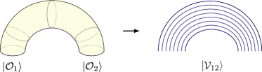
Figure 1: The two point correlation function and $|{\cal V}_{12}\rangle$

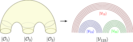
Figure 2: The three point correlation function and $|{\cal V}_{123}\rangle$

The same strategy can be used to reformulate the three point function,

$$\langle{\cal O}_{2}(y){\cal O}_{3}(z){\cal O}_{1}(x)\rangle=\langle{\cal V}_{123}|\,e^{i(L^{+}_{1}x+L^{+}_{2}y+L^{+}_{3}z)}|{\mathcal{O}}_{2}\rangle\otimes|{\mathcal{O}}_{3}\rangle\otimes|{\cal O}_{1}\rangle\,,$$ (8)

using the three-point invariant $|{\cal V}_{123}\rangle$ defined, at tree level, as

$$|{\cal V}_{123}\rangle=|{\cal V}_{12}\rangle\otimes|{\cal V}_{13}\rangle\otimes|{\cal V}_{32}\rangle\;.$$ (9)

The objects entering the correlation functions are schematically depicted in figures 1 and 2. Such an interpretation of the correlation functions is close in spirit to the construction in Koch:2014nka , but it is also heavily inspired from the ideas in string field theory, where the object similar to $|{\cal V}_{123}\rangle$ is the string vertex Spradlin:SFT2 ; Spradlin:SFT1 ; Pankiewicz:2002tg ; Shimada:2004sw ; Dobashi:Resolving ; Klose:lightcone3pt ; Shulgin-Zayakin .

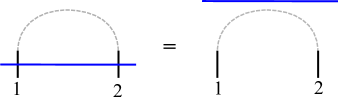
Figure 3: The basic relation of vertex operator, the two states connected by the dashed line is identified.

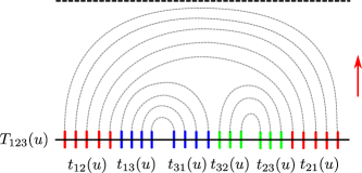
Figure 4: The three-point spin vertex and monodromy condition.

Compared to the previous works, the step forward we take here is to reformulate the local symmetry (6) as a non-local symmetry realized by the Yangian. Of course, our aim is to reformulate the symmetry conditions for the three point functions at arbitrary coupling in terms of integrability. Here, we show that at the tree level the spin vertex $|{\cal V}_{123}\rangle$ is a Yangian invariant,

$$T_{123}(u)|{\cal V}_{123}\rangle=|{\cal V}_{123}\rangle\;,$$ (10)

with the monodromy matrix $T^{(123)}(u)$ built from the pieces of the three chains, as shown in figure 4,

$$T_{123}(u)=t^{(12)}(u)\,t^{(13)}(u)\,t^{(31)}(u)\,t^{(32)}(u)\,t^{(23)}(u)\,t^{(21)}(u)\;.$$ (11)

The building block used for the monodromy condition is property of the two-site vertex $|{\cal V}_{12}\rangle$ carrying on the sites $1$ and $2$ the physical representation, as represented schematically in figure 3,

$$R_{01}(u)R_{02}(u)|{\cal V}_{12}\rangle=|{\cal V}_{12}\rangle\;.$$ (12)

This relation can be traced back to the unitarity property of the $R$ matrix, $R_{01}(u)R_{01}(-u)=1$, plus a version of the crossing relation mediated by the vertex. Let us mention that the specific form of the monodromy property (12) concerns the full $\mathfrak{psu}(2,2|4)$ R matrix and it changes when reduced to particular subsectors. The integrable structure displayed by the vertex is instrumental in computing even the tree-level correlation functions ShotaNew , some of which were known previously. We think that the integrable structure will be maintained at higher loops, and that the integrability constraints combined with few general constraints will be sufficient to determine the three point function, very much as the integrability constraints were sufficient to determine the spectrum of anomalous dimensions Beisert-Rev .

The structure of the paper is as follows: in section 2 we are reviewing the oscillator representation for the tree level $\mathfrak{psu}(2,2|4)$ algebra, as well as the ADGN approach to computing the correlation functions using the Fock space representation and the vertex. In section 3 we construct the spin vertex at tree level and we characterize its properties, in particular how it flips outgoing states into incoming states. The subsection 3.2.2 shows how to reduce the computation of correlation functions in the $\mathfrak{so}(6)$ sector to overlaps, and how to retrieve the results obtains by EGSV EGSV . In section 4 we formulate the monodromy condition and verify that it is satisfied for the auxiliary space in the defining representation. We end with conclusions and some comments about the extension of the results at higher loops.

Note: We acknowledge that a part of the subjects discussed in this paper is also investigated independently in the paper by Y. Kazama, S. Komatsu and T. Nishimura Shota1:Yangian . Partial results of the two groups were presented at the APCTP workshop in Pohang ShotaPohang ; DidinaPohang .

2 Oscillator representation and the free ${\cal N}=4$ SYM

In determining the spectrum, the spin chain representation of the dilation operator was very important. This representation can be easily understood using the oscillator representation of the algebra $\mathfrak{psu}(2,2|4)$ Gunaydin1 ; Gunaydin2 ; Beisert-thesis . The oscillator representation, valid for the free field theory, is a good starting point for setting up the perturbation theory. The same representation is also useful in computing the correlation functions, since our aim is to reduce the computation of structure constants to the evaluation of overlaps of wave functions of the spin chains. In this section we are reviewing the link between the oscillator representation of $\mathfrak{psu}(2,2|4)$ and the standard unitary presentation of the super-conformal group, link which is explained at length in the reference ADGN . We refer to this article for further details.

Let us first discuss the oscillator representation of the compact version of $\mathfrak{psu}(2,2|4)$, $\mathfrak{psu}(4|4)$. It uses four copies of bosonic oscillators, $a_{i},b_{i},\ i=1,2$ and four copies of fermionic oscillators, $c_{k},\ k=1,\ldots,4$,

$$[a_{i},a_{j}^{\dagger}]=\delta_{ij}\;,\quad[b_{i},b_{j}^{\dagger}]=\delta_{ij}\;,\quad\{c_{k},c_{l}^{\dagger}\}=\delta_{kl}\;,\quad i,j=1,2\;,\quad k,l=1,\ldots,4\;.$$ (13)

We organize the oscillators in a eight-dimensional vector

$$\phi=(\begin{array}[]{ccc}a_{i}&b_{i}&c_{k}\end{array})$$ (15)

such that the generators of $\mathfrak{u}(4|4)$ can be written as

$$E^{AB}_{\rm compact}=\phi^{A\dagger}\phi^{B}\quad{\rm with}\quad E^{AB\dagger}_{\rm compact}=E^{BA}_{\rm compact}\;.$$ (16)

It is straightforward to check that they satisfy the commutation relations of the $\mathfrak{u}(4|4)$ algebra,

$$[E^{AB},E^{CD}]=\delta^{BC}E^{AD}-(-1)^{(|A|+|B|)(|C|+|D|)}\delta^{AD}E^{CB}\;,$$ (17)

with $[\cdot,\cdot]$ meaning commutator or anti-commutator, depending on the grading of the generators, and the grading is $|A|=0,1$ for bosonic and fermionic indices respectively. The non-compact form $\mathfrak{u}(2,2|4)$ can be obtained after a particle-hole transformation for one group of bosonic oscillators, say $b$,

$$E^{AB}=E^{AB}_{\rm compact}(b\to-b^{\dagger},b^{\dagger}\to b)\;.$$ (18)

The commutation relations (17) are preserved by the particle-hole transformation, but the Hermitian conjugate of the generators are now

$$\ E^{AB\dagger}=\gamma\,E^{BA}\gamma\;,\qquad\gamma={\rm diag}(1_{2},-1_{2},1_{4})\;.$$ (19)

Sometimes, for the sake of symmetry, it is convenient to perform also a particle-hole transformation of the fermionic oscillators

$$d_{i}=c_{i+2}^{\dagger}\;,\qquad d_{i}^{\dagger}=c_{i+2}\,\quad i=1,2\;.$$ (20)

Unlike the bosonic particle-hole transformation, the fermionic one is unitary and therefore it does not change the real form of the algebra. We will use alternatively the two notations. The Lie-algebra generators are expressed in terms of these oscillators as

$$E^{AB}=\bar{\psi}^{A}\psi^{B}\;,$$ (21)

with

$$\psi=(\begin{array}[]{cccc}a_{i}&\ -b^{\dagger}_{i}&\ c_{i}&\ d^{\dagger}_{i}\end{array}),\quad\bar{\psi}=\psi^{\dagger}\gamma=(\begin{array}[]{cccc}a_{i}^{\dagger}&\ b_{i}&\ c_{i}^{\dagger}&\ d_{i}\end{array}).$$ (24)

The projective condition in $\mathfrak{psu}(2,2|4)$ is obtained by imposing that the identity generator $\sum_{A}E^{AA}=\bar{\psi}\psi$, a central charge of the algebra, is zero,

$$\sum_{A}E^{AA}=\sum_{i=1,2}(N_{a_{i}}-N_{b_{i}}+N_{c_{i}}+N_{c_{i+2}}-1)=\sum_{i=1,2}(N_{a_{i}}-N_{b_{i}}+N_{c_{i}}-N_{d_{i}})=0\;,$$ (25)

where $N_{a},\ N_{b},\ N_{c},\ N_{d}$ are the number of the respective types of bosons and fermions in the two types of representations. The above condition selects two types of modules, lowest weight $V_{+}$ and highest weight $V_{-}$, built upon two vacua $|0\rangle$ and $|\bar{0}\rangle$ respectively, dual to each other

$$|0\rangle=|0\rangle_{B}\otimes|0\rangle_{F}\;, \qquad|\bar{0}\rangle=|\bar{0}\rangle_{B}\otimes|\bar{0}\rangle_{F}\;,$$ (26)

$$(a_{i},b_{i},c_{i},d_{i})|0\rangle=0\;, \qquad(a_{i}^{\dagger},b_{i}^{\dagger},c_{i}^{\dagger},d_{i}^{\dagger})|\bar{0}\rangle=0\;,\quad i=1,2\;.$$

It is worth mentioning that the particle-hole transformation $(a_{i},b_{i},c_{i},d_{i})\to(-a_{i}^{\dagger},-b_{i}^{\dagger},c_{i}^{\dagger},d_{i}^{\dagger})$ and $(a_{i}^{\dagger},b_{i}^{\dagger},c_{i}^{\dagger},d_{i}^{\dagger})\to(a_{i},b_{i},c_{i},d_{i})$ helps defining another copy of the $\mathfrak{psu}(2,2|4)$ generators that act naturally in the dual module $V_{-}$ and which are the particle-hole transformed of the generators (21). The new generators can be shown to be equal to

$$\bar{E}^{AB}=-(-1)^{|B|}\psi^{A}\bar{\psi}^{B} =-(-1)^{|B|+|A||B|}E^{BA}-(-1)^{|B|}\delta^{BA}$$

$$=-(E^{AB}+(-1)^{|B|}\delta^{BA})^{t}\;,$$ (27)

where the index ^t stands for the super transposition.

Let us now concentrate on the conformal subalgebra in four dimensions $\mathfrak{so}(2,4)\simeq\mathfrak{su}(2,2)$. In the above oscillator representation, there is a natural grading with respect to the maximal compact subalgebra $\mathfrak{u}(1)\otimes\mathfrak{su}(2)\otimes\mathfrak{su}(2)$. The grading is given by the value of the $\mathfrak{u}(1)$ generator $E$

$$[E,L^{\pm}] =\pm L^{\pm}\;,\qquad[E,L^{0}]=0\;.$$

In other words, the generators $L^{0}$ from the maximal compact subgroup preserve the number of bosons, while $L^{\pm}$ increase or decrease the number of bosons by 2. We are going to use later the explicit representation of these operators in terms of oscillators,

$$E=1 +{\textstyle{1\over 2}}(N_{a}+N_{b})={\textstyle{1\over 2}}(a^{\dagger}a+bb^{\dagger})\;,$$ (28)

$$L_{\mu}^{+} =-a^{\dagger}\bar{\sigma}_{\mu}b^{\dagger}\;,\quad L_{\mu}^{-}=b\sigma_{\mu}a\;,$$ (29)

with $\sigma_{\mu}=(-1,\vec{\sigma})$, and $\bar{\sigma}_{\mu}=(-1,-\vec{\sigma})$ and summation over indices of the bosonic operators is understood. For the $R$ charge sector, the generators are those of the $\mathfrak{su}(4)$ algebra

$${\rm R}^{kl}=c_{k}^{\dagger}c_{l}-\frac{1}{4}\delta_{kl}\,c^{\dagger}c\;.$$ (30)

We will now identify the above generators with the standard presentation of the conformal group, which is the group of rotations in a six-dimension space with signature $\eta_{PQ}={\rm diag}(-++++-)$. We adopt the same convention as in ADGN and call the directions in the six-dimensional space $P,Q=0,1,2,3,5,6$, with the first four directions corresponding to the Minkovski space, $\mu,\nu=0,1,2,3$ . The commutation relation are

$$[M_{PQ},M_{RS}]=i(\eta_{QR}M_{PS}-\eta_{PR}M_{QS}-\eta_{QS}M_{PR}+\eta_{PS}M_{QR})\;,$$ (31)

and the identification of the generators for translations $P_{\mu}$, special conformal transformations $K_{\mu}$ and dilatation $D$ is made as

$$P_{\mu}=M_{\mu 6}+M_{\mu 5}\;,\qquad K_{\mu}=M_{\mu 6}-M_{\mu 5}\;,\qquad D=-M_{56}\;.$$ (32)

On the other hand, the $\mathfrak{u}(1)$ generator in the oscillator representation $E$ is given by

$$E=M_{06}={\textstyle{1\over 2}}(P_{0}+K_{0})\;.$$ (33)

The authors of ADGN suggested that the oscillator representation and the standard representation above can be related by a transformation which exchanges the two directions with opposite signature $0$ and $5$, that is a rotation with an imaginary angle $-i\pi/2$ in the plane $05$,

$$U=\exp-\frac{\pi}{2}M_{05}=\exp-\frac{\pi}{4}(P_{0}-K_{0})\;,$$ (34)

and its action translates into

$$U^{-1}K_{\mu}U=L_{\mu}^{-}\;,\quad U^{-1}P_{\mu}U=L_{\mu}^{+}\;,\quad U^{-1}DU=iE\;,$$ (35)

$$L_{0}^{+}-L_{0}^{-}=U^{-1}(P_{0}-K_{0})U=P_{0}-K_{0}\;,$$ (36)

which helps make contact between rotated and unrotated representations. The transformation implemented by $U$ is similar to the so-called mirror transformation in two-dimensional field theories, including the AdS/CFT sigma model. From the space-time interpretation, it is obvious that this transformation should obey $U^{4}=1$ except on spinors, and that $U^{2}$ is a kind of PT transformation which changes the sign of both 0 and 5 coordinates,

$$U^{-2}DU^{2}=-D\;,\qquad U^{-2}EU^{2}=-E\;.$$ (37)

This relation is purely algebraic and it holds at any loop level, as it can be seen putting

$$U_{t}=\exp\frac{t}{2}(P_{0}-K_{0})\;,\qquad D_{t}=U_{t}^{-1}DU_{t}\;,\qquad E_{t}=U_{t}^{-1}EU_{t}\;.$$

Taking the derivative with respect to $t$ and using $E=\frac{1}{2}(P_{0}+K_{0})$ and $D=\frac{i}{2}[P_{0},K_{0}]$ and the commutation relations of the conformal algebra, we get $\partial_{t}E_{t}=iD_{t}$ and $\partial_{t}D_{t}=iE_{t}$, which is solved by

$$D_{t}=D\cos t+iE\sin t\;,\qquad E_{t}=E\cos t+iD\sin t\;.$$ (38)

At tree level, the oscillator representation of the hermitian operator $U$ is

$$U=\exp-\frac{\pi}{4}\sum_{i=1,2}(a^{\dagger}_{i}b^{\dagger}_{i}+a_{i}b_{i})\;,\qquad U^{\dagger}=U\;.$$ (39)

By inspection, using the oscillator representation, we find that

$$U^{2}L_{\mu}^{+}U^{-2}=- b\bar{\sigma}_{\mu}a\;,\qquad U^{2}L_{\mu}^{-}U^{-2}=a^{\dagger}\sigma_{\mu}b^{\dagger}\;,\quad{\rm or}$$ (40)

$$U^{2}L_{0}^{\pm}U^{-2} =-L_{0}^{\mp}\;,\qquad U^{2}L_{m}^{\pm}U^{-2}=L_{m}^{\mp}\;,$$

$$U^{2}P_{0}U^{-2} =-K_{0}\;,\qquad U^{2}P_{m}U^{-2}=K_{m}\;.$$

These relations can be derived using the action of the operator $U$ on the oscillators, in particular

$$U^{2}aU^{-2}=b^{\dagger}\;,\quad U^{2}a^{\dagger}U^{-2}=-b\;,\quad U^{2}b\,U^{-2}=a^{\dagger}\;,\quad U^{2}b^{\dagger}U^{-2}=-a\;.$$ (41)

From here we conclude also that the transformation $U^{2}$ sends the bosonic Fock vacuum $|0\rangle_{B}$ into the dual vacuum $|\bar{0}\rangle_{B}$,

$$|\bar{0}\rangle_{B}=U^{2}|0\rangle_{B}\;,\qquad a^{\dagger},b^{\dagger}|\bar{0}\rangle_{B}=0\;,$$ (42)

therefore mapping the lowest weight module $V_{+}$ to the highest weight one $V_{-}$ and back,

$$V_{+}\ {\buildrel U^{2}\over{\longleftrightarrow}}\ V_{-}\;.$$ (43)

Given the relation (37), we may conclude that the positive energy states belong to $V_{+}$ and the negative energy ones belong to $V_{-}$, where the term of energy refers to the eigenvalues of the operater $E$. We note from the relations (41) that

$$U^{-4}x\,U^{4}=-x,\qquad x=a_{i},a_{i}^{\dagger},b_{i},b_{i}^{\dagger}\;,$$ (44)

which does not pose a problem for the generators which are quadratic in the bosons or in the fermions, but it changes the sign of the odd generators of the super-conformal group, which transform in the spinorial representations of both $\mathfrak{so}(6)$ and $\mathfrak{so}(4,2)$. Therefore, we may supplement the operator $U$ with a fermionic counterpart $U_{F}$, such that ${\rm U}=(UU_{F})^{4}$ will change the sign of the fermions as well,

$$U_{F}=\exp-\frac{\pi}{4}\sum_{i=1,2}(c_{i}^{\dagger}d_{i}^{\dagger}+c_{i}d_{i})\;,\qquad U_{F}^{\dagger}=U_{F}^{-1}\;.$$ (45)

In other words, the non-unitary rotation in space-time is supplemented by an unitary rotation in the $R$ charge sector, which is the product of two $\mathfrak{su}(2)$ rotations that will be called later $\mathfrak{su}(2)_{L}$ and $\mathfrak{su}(2)_{R}$. The action of the transformation on the fermionic oscillators is

$$U_{F}^{2}c_{i}\,U_{F}^{-2}=d_{i}^{\dagger},\quad U_{F}^{2}c_{i}^{\dagger}\,U_{F}^{-2}=d_{i},\quad U_{F}^{2}d_{i}\,U_{F}^{-2}=-c_{i}^{\dagger},\quad U_{F}^{2}d^{\dagger}_{i}\,U_{F}^{-2}=-c_{i}$$

$$U_{F}^{4}x\,U_{F}^{-4}=-x,\qquad x=c_{i},c_{i}^{\dagger}\,d_{i},d_{i}^{\dagger}\,$$ (46)

$$\qquad U_{F}^{-2}\equiv\sigma=-\sigma_{2,L}\,\sigma_{2,R}$$

and it also transforms the fermionic vacuum into its conjugate,

$$|\bar{0}\rangle_{F}=U_{F}^{2}|0\rangle_{F}\equiv U_{F}^{2}|Z\rangle=c_{1}^{\dagger}d_{1}^{\dagger}c_{2}^{\dagger}d_{2}^{\dagger}|0\rangle_{F}\equiv|\bar{Z}\rangle\;.$$ (47)

Let us note that $U_{F}^{2}$, being a rotation, maps $V_{\pm}$ to themselves,

$$V_{\pm}\ {\buildrel U_{F}^{2}\over{\longleftrightarrow}}\ V_{\pm}\;.$$ (48)

2.1 Oscillator representation and the correlation functions

We have now the necessary ingredients to present the dictionary between the gauge invariant operators in the conformal field theory and the Fock space representation. The gauge invariant operators we will consider in the planar limit are the single traces on the gauge group, or “words” made up from the “letters” which are the fundamental fields of the theory – and which were interpreted as string bits in view of the gauge-string correspondence,

$${\mathcal{O}}(x)\sim{\rm Tr}(XXZY\Psi_{i}\ldots)(x)\;.$$ (49)

When the gauge coupling constant is zero, these string bits are independent and each of them is in a state corresponding to the $\mathfrak{psu}(2,2|4)$ representation described above. Gauge invariant operators can then be represented by elements in the tensor product of the individual string bits. In the spin chain representation, string bits are the sites of the spin chain, and we will have to introduce a copy of oscillators on each site $s$,

$$\psi_{s}=\left(\begin{array}[]{cccc}a_{i,s}&-b^{\dagger}_{i,s}&c_{i,s}&d^{\dagger}_{i,s}\end{array}\right)\;,\quad s=1,\ldots,L\;$$ (51)

acting in the tensor product of individual sites $V_{\pm}^{\otimes L}=V_{1,\pm}\otimes\dots\otimes V_{L,\pm}$. In the non-interacting gauge theory, the oscillator representation of the super-conformal group generators will be

$$E^{AB}=\sum_{s=1}^{L}E^{AB}_{s}\;,\quad{\rm U}={\rm U}_{1}\otimes\dots\otimes{\rm U}_{L},$$ (52)

while the radiative correction will introduce interaction between the string bits, or sites. The space of conformal primary operators ${\cal O}(x)$ situated at $x=0$ is selected by the condition

$$K_{\mu}{\cal O}(0)=0\;.$$ (53)

On the other hand, we have for the Fock vacuum $|0\rangle=|0\rangle_{1}\otimes\dots\otimes|0\rangle_{L}$

$$L^{-}_{\mu}|0\rangle=0\;,\quad{\rm hence}\quad K_{\mu}U|0\rangle=0\;.$$ (54)

Similarly, following ADGN , we can relate the space of conformal primary operators with the space of Fock states $|{\cal O}\rangle$ annihilated by the $L^{-}_{\mu}$ operator,

$$L^{-}_{\mu}|{\cal O}\rangle=0\;,\quad\Rightarrow\quad K_{\mu}U|{\cal O}\rangle=0\;.$$ (55)

Translating the operators to a different space-time point can be done with the help of the momentum operator,

$${\cal O}(x)=e^{iPx}{\cal O}(0)e^{-iPx}\;,$$ (56)

with corresponding Fock space representative

$$e^{iPx}U|{\cal O}\rangle\;.$$ (57)

For the operators ${\mathcal{O}}$ with definite conformal dimension $\Delta$ we have

$$D\,U|{\cal O}\rangle=i\,UE|{\cal O}\rangle=i\,\Delta\,U|{\cal O}\rangle\;,$$ (58)

so that

$$e^{iD\ln\Lambda}U|{\cal O}\rangle=\Lambda^{-\Delta}\,U|{\cal O}\rangle\;.$$ (59)

A similar identification holds between the bra states and the hermitian conjugates of the operators,

$${\cal O}^{\dagger}(x)\quad\longleftrightarrow\quad\langle{\cal O}|U^{\dagger}e^{-iPx}=\langle{\cal O}|U^{\dagger}e^{-iPx}\;.$$ (60)

This mapping was used by the authors of ADGN to write the two point function in terms of the Fock space representation,

$$\langle{\cal O}_{2}^{\dagger}(y){\cal O}_{1}(x)\rangle=\langle{\cal O}_{2}|U^{\dagger}e^{iP(x-y)}U|{\cal O}_{1}\rangle=\langle{\cal O}_{2}|U^{2}e^{iL^{+}(x-y)}|{\cal O}_{1}\rangle\;.$$ (61)

The authors of ADGN also verified that if ${\cal O}$ is any elementary field, for example $Z$, the tree-level representation of the operators in the Fock space gives the desired result of the Wick contraction

$$\langle\bar{Z}(x){Z}(y)\rangle=\langle Z|U^{2}e^{iL^{+}(y-x)}|Z\rangle=\frac{\langle Z|Z\rangle}{(x-y)^{2}}=\frac{1}{(x-y)^{2}}\;.$$ (62)

To get the next to the last equality sign, one has to use $L^{+}_{\mu}=-a^{\dagger}\bar{\sigma}_{\mu}b^{\dagger}$ and, as suggested in ADGN , to regularise $U^{2}$ as $U^{2}=\lim_{t\to-\pi/2}U_{t}$, with $U_{t}$ given by

$$U_{t}=\exp t(a^{\dagger}b^{\dagger}+ba)=\exp(a^{\dagger}b^{\dagger}\tan t)\exp(-(a^{\dagger}a+bb^{\dagger})\ln\cos t)\exp(ab\tan t)\;.$$ (63)

(We give the details in Appendix A.) In fact, the relation above should hold at higher loop as well,

$$U_{t}=\exp-t(L_{0}^{+}-L_{0}^{-})=\exp(-L_{0}^{+}\tan t)\exp(-2E\ln\cos t)\exp(L_{0}^{-}\tan t)\;,$$ (64)

since the commutation relations $[E,L_{0}^{\pm}]=\pm L_{0}^{\pm}$ and $2E=[L_{0}^{+},L_{0}^{-}]$ are the same at any coupling. The last equality sign in (62) amounts to computing the overlap for the vacuum state,

$$\langle Z|Z\rangle=1\;,\qquad|Z\rangle=|0\rangle\;.$$ (65)

A similar representation can be used for the special case of the extremal three point function, when the length of the first chain equal the sum of the lengths of the second and the third, $L_{1}=L_{2}+L_{3}$,

$$\langle{\cal O}_{2}^{\dagger}(y){\cal O}_{3}^{\dagger}(z){\cal O}_{1}(x)\rangle_{\rm ext}=\langle{\cal O}_{2}|\otimes\langle{\cal O}_{3}|U_{2}U_{3}\,e^{iP_{1}x}e^{-iP_{3}z}e^{-iP_{2}y}U_{2}|{\cal O}_{1}\rangle_{\rm ext}\;,$$ (66)

where the index on the operators shows now the space on which they act. At tree level for the extremal correlator $U_{1}=U_{2}U_{3}$ and $P_{1}=P_{2}+P_{3}$. We conclude from the above that the correlators in the Fock space representation involve a pairing between states in the $V_{+}$ module in the ket states and the $V_{-}$ module in the bra states.

2.2 The necessity of the spin vertex

The Fock space representation is easily understood for the two point function and the extremal three point function, where at weak coupling the number of sites (string bits) is conserved from the bra to the ket states. The situation is more subtle for non-extremal correlation functions, where the chains are splitting and joining, and some pieces of the chains have to be flipped (see e.g. EGSV ) in order to contract them with pieces of a different chain. Let us now interpret the two point correlator in (61) in a slightly different manner, considering now that both operators act on the left Fock space. To do this, we need a mapping from a left state $\langle{\cal O}|$, to a right state $|\bar{\mathcal{O}}\rangle$, which will be done via a specially prepared state $\langle V_{12}|$ which lives in the tensor product of two chains,

$$\;^{(1)}\langle{\cal O}|=\langle V_{12}|\,\sigma^{(1)}\,|\bar{\mathcal{O}}\rangle^{(2)}\;,\qquad\sigma\equiv U_{F}^{-2},$$ (67)

where we have added an index to the Fock spaces to emphasize that $\langle{\cal O}|$ and $|\bar{\mathcal{O}}\rangle$ live in different modules $(V_{+}^{\otimes L})^{(1)}$ and $(V_{+}^{\otimes L})^{(2)}$ intertwined by $\langle V_{12}|$. We will show in section 3.2.1 that the state $|\bar{\mathcal{O}}\rangle$ is the flipped state with respect to $\langle{\cal O}|$ in the sense of EGSV , being different from $|{\cal O}\rangle$. In this language, the two point function is

$$\langle{\cal O}_{2}^{\dagger}(y){\cal O}_{1}(x)\rangle =\langle V_{12}|\,{\rm U}_{(1)}^{\dagger 2}\;e^{iL^{+}_{(1)}(x-y)}\,|{\bar{\mathcal{O}}}_{2}\rangle^{(2)}\otimes|{\mathcal{O}}_{1}\rangle^{(1)}$$

$$=\langle{\cal V}_{12}|\,e^{iL^{+}_{(1)}(x-y)}\,|{\bar{\mathcal{O}}}_{2}\rangle^{(2)}\otimes|{\mathcal{O}}_{1}\rangle^{(1)}$$

$$=\langle{\cal V}_{12}|\,e^{i[L^{+}_{(1)}x+L^{+}_{(2)}y]}\,|{\bar{\mathcal{O}}}_{2}\rangle^{(2)}\otimes|{\mathcal{O}}_{1}\rangle^{(1)}\;,$$ (68)

where ${\rm U}^{2}=U^{2}U_{F}^{2}$ and ${\rm U}^{{\dagger}2}=U^{2}U_{F}^{-2}$. In the second line we have introduced the state

$$\langle{\cal V}_{12}|\equiv\langle V_{12}|\,{\rm U}_{(1)}^{{\dagger}2}\;,\qquad|{\cal V}_{12}\rangle\in V_{-}^{\otimes L}\otimes V_{+}^{\otimes L}\;,$$ (69)

and used the property which we will prove later

$$\langle V_{12}|\,{\rm U}_{(1)}^{{\dagger}2}\,(L_{(1)}^{+}+L_{(2)}^{+})\equiv\langle{\cal V}_{12}|(L_{(1)}^{+}+L_{(2)}^{+})=0\;.$$ (70)

The state $\langle{\cal V}_{12}|$, or its conjugate $|{\cal V}_{12}\rangle$, should play the role of the vacuum state, in the sense that is has to carry the same quantum numbers as the vacuum. It is clear that $|{\cal V}_{12}\rangle$ cannot be the tensor product of the Fock space vacua of the two chains. At tree level, $|{\cal V}_{12}\rangle$ should provide the right Wick contractions between the elementary fields in ${\mathcal{O}}_{2}^{\dagger}$ and ${\mathcal{O}}_{1}$. A similar relation holds for the extremal three point function,

$$\langle{\cal O}^{\dagger}_{2}(y){\cal O}^{\dagger}_{3}(z){\cal O}_{1}(x)\rangle_{\rm ext} =\,_{\rm ext}\langle V_{123}|\,{\rm U}_{(1)}^{\dagger 2}\;e^{i[L^{+}_{(1)}x+L^{+}_{(2)}y+L^{+}_{(3)}z]}|\bar{\mathcal{O}}_{2}\rangle\otimes|\bar{\mathcal{O}}_{3}\rangle\otimes|{\cal O}_{1}\rangle$$ (71)

$$=\,_{\rm ext}\langle{\cal V}_{123}|\,e^{i[L^{+}_{(1)}x+L^{+}_{(2)}y+L^{+}_{(3)}z]}|\bar{\mathcal{O}}_{2}\rangle\otimes|\bar{\mathcal{O}}_{3}\rangle\otimes|{\cal O}_{1}\rangle\,,$$

where the extremal vertex $|{\cal V}_{123}\rangle_{\rm ext}$ is built from two pieces connecting each the operators ${\mathcal{O}}_{2}$ and ${\mathcal{O}}_{3}$ with ${\mathcal{O}}_{1}$,

$$|{\cal V}_{123}\rangle_{\rm ext}=|{\cal V}_{12}\rangle\otimes|{\cal V}_{13}\rangle\;.$$ (72)

In this case, at tree level there are Wick contractions only between the operators 1 and 2 and 1 and 3 and there are no contractions between the operators 2 and 3. At this point we are starting to see that in the vertex formulation the operators can be treated more democratically,

$$\langle{\cal O}_{2}(y){\cal O}_{3}(z){\cal O}_{1}(x)\rangle_{\rm ext}=\,_{\rm ext}\langle{\cal V}_{123}|\,e^{i[L^{+}_{(1)}x+L^{+}_{(2)}y+L^{+}_{(3)}z]}|{\mathcal{O}}_{2}\rangle\otimes|{\mathcal{O}}_{3}\rangle\otimes|{\cal O}_{1}\rangle\;.$$ (73)

This helps to define the slightly more complicated case of a non-extremal three point function, where the operators ${\mathcal{O}}_{2}$ and ${\mathcal{O}}_{3}$ are also connected by Wick contractions. At tree level, we can split any of the operators ${\mathcal{O}}_{i}$ into pieces ${\mathcal{O}}_{ij}$ which are contracted to pieces ${\mathcal{O}}_{ji}$ of operator ${\mathcal{O}}_{j}$. At the level of the states we have

$$|{\mathcal{O}}_{1}\rangle=|{\mathcal{O}}_{13}\rangle\otimes|{\mathcal{O}}_{12}\rangle\;,$$ (74)

$$|{\mathcal{O}}_{2}\rangle=|{\mathcal{O}}_{21}\rangle\otimes|{\mathcal{O}}_{23}\rangle\;,$$

$$|{\mathcal{O}}_{3}\rangle=|{\mathcal{O}}_{32}\rangle\otimes|{\mathcal{O}}_{31}\rangle\;.$$

The non-extremal three point function, at tree level, can be then written in the same way as non-extremal, but with another definition of the vertex

$$\langle{\cal O}_{2}(y){\cal O}_{3}(z){\cal O}_{1}(x)\rangle=\langle{\cal V}_{123}|\,e^{i[L^{+}_{(1)}x+L^{+}_{(2)}y+L^{+}_{(3)}z]}|{\mathcal{O}}_{2}\rangle\otimes|{\mathcal{O}}_{3}\rangle\otimes|{\cal O}_{1}\rangle\,,$$ (75)

with the vertex $|{\cal V}_{123}\rangle$ built out as

$$|{\cal V}_{123}\rangle =|{\cal V}_{12}\rangle\otimes|{\cal V}_{13}\rangle\otimes|{\cal V}_{32}\rangle={\rm U}^{2}_{(12)}|V_{12}\rangle\otimes{\rm U}^{2}_{(13)}|V_{13}\rangle\otimes{\rm U}^{2}_{(32)}|V_{32}\rangle\;\;,$$

$$|{\cal V}_{ij}\rangle \in V_{-}^{\otimes L_{ij}}\otimes V_{+}^{\otimes L_{ji}}\;.$$ (76)

The construction of the states $|{\cal V}_{12}\rangle$ and $|{\cal V}_{123}\rangle$, that we call the spin vertex (by abuse of language we will call $|{\cal V}_{12}\rangle$ the two-vertex) is the main purpose of this work.

3 The spin vertex at tree level

In this section we are defining the basic building blocks we need to build the vertex at tree level. The main object is the two-vertex $|{\cal V}_{12}\rangle$, which is an invariant of the $\mathfrak{su}(2,2|4)$ algebra and which can be therefore used as a “vacuum state” in the tensor product of multiple Fock spaces when we compute the correlation functions.

3.1 Definition of the two-vertex

We will concentrate first on the case of the two-vertex $|{\cal V}_{12}\rangle$ and infer the properties required such that (61) and (2.2) are identical. A construction of the vertex using the oscillator representation was given in ADGN . Here we give a slightly modified version of that construction

$$|{\cal V}_{12}\rangle \equiv{\rm U}_{(1)}^{2}|{V}_{12}\rangle$$

$$={\rm U}_{(1)}^{2}\exp\sum_{s=1}^{L}\sum_{i=1,2}\left(b^{(1)\dagger}_{i,s}a^{(2)\dagger}_{i,s}-a^{(1)\dagger}_{i,s}b^{(2)\dagger}_{i,s}-d^{(1)\dagger}_{i,s}c^{(2)\dagger}_{i,s}-c^{(1)\dagger}_{i,s}d^{(2)\dagger}_{i,s}\right)|0\rangle^{(2)}\otimes|0\rangle^{(1)}$$

$$=\exp-\sum_{s=1}^{L}\sum_{i=1,2}\left(a^{(1)}_{i,s}a^{(2)\dagger}_{i,s}-b^{(1)}_{i,s}b^{(2)\dagger}_{i,s}+d^{(1)}_{i,s}d^{(2)\dagger}_{i,s}-c^{(1)}_{i,s}c^{(2)\dagger}_{i,s}\right)|0\rangle^{(2)}\otimes|\bar{0}\rangle^{(1)}\;,$$ (77)

where the upper index on the oscillators indicates the Fock space where they act, and $|\bar{0}\rangle={\rm U}^{2}|0\rangle$. In order to mimic the planar contractions we revert the order of the tensor product in the second chain,

$$|0\rangle^{(2)}\otimes|0\rangle^{(1)}=\left(|0\rangle_{L}^{(2)}\otimes\dots\otimes|0\rangle_{1}^{(2)}\right)\otimes\left(|0\rangle_{1}^{(1)}\otimes\ldots\otimes|0\rangle_{L}^{(1)}\right)\;.$$ (78)

The vertex (3.1) can be expanded as

$$|{\cal V}_{12}\rangle =\sum_{N_{a},N_{b},N_{c},N_{d}}|N_{a},N_{b},N_{c},N_{d}\rangle^{(2)}\otimes|\bar{N}_{a},\bar{N}_{b},\bar{N}_{c},\bar{N}_{d}\rangle^{(1)}$$ (79)

$$=\sum_{N_{a},N_{b},N_{c},N_{d}}|\bar{N}_{a},\bar{N}_{b},\bar{N}_{c},\bar{N}_{d}\rangle^{(2)}\otimes|N_{a},N_{b},N_{c},N_{d}\rangle^{(1)}=(-1)^{F}|{\cal V}_{21}\rangle\ \;,$$

where $F=N_{c}+N_{d}$ is the number of fermions and

$$|N_{a},N_{b},N_{c},N_{d}\rangle= \frac{1}{\sqrt{N_{a}!\,N_{b}!}}\prod_{k=1,2}(d_{k}^{\dagger})^{N_{d_{k}}}(c_{k}^{\dagger})^{N_{c_{k}}}(b_{k}^{\dagger})^{N_{b_{k}}}(a_{k}^{\dagger})^{N_{a_{k}}}|0\rangle\;,$$ (80)

$$|\bar{N}_{a},\bar{N}_{b},\bar{N}_{c},\bar{N}_{d}\rangle =\frac{(-1)^{N_{a}+N_{c}}}{\sqrt{N_{a}!\,N_{b}!}}\prod_{k=1,2}a_{k}^{N_{a_{k}}}b_{k}^{N_{b_{k}}}c_{k}^{N_{c_{k}}}d_{k}^{N_{d_{k}}}|\bar{0}\rangle\;,$$

with $N_{a}!\equiv N_{a_{1}}!\,N_{a_{2}}!$ and $N_{b}!\equiv N_{b_{1}}!\,N_{b_{2}}!$. For the states containing fermions one should take care of signs, so the order on which the fermionic oscillators act is important. In the formulas above we take the convention that the oscillators act in opposite order on the two chains. One can easily project the vertex in (79) on the states obeying $N_{a}-N_{b}+N_{c}-N_{d}=0$. The second line in (79) can be proven using

$${\rm U}_{(1)}|V_{12}\rangle={\rm U}_{(2)}^{-1}|V_{12}\rangle\;,\qquad{\rm U}_{(1)}|{\cal V}_{12}\rangle={\rm U}_{(2)}^{-1}|{\cal V}_{12}\rangle\;,$$ (81)

which will can be shown using the properties (3.1) below. From the oscillator expansion (79) it can be readily seen that

$$\langle{\cal V}_{31}|{\cal V}_{12}\rangle=\sum_{N_{a},N_{b},N_{c},N_{d}}|N_{a},N_{b},N_{c},N_{d}\rangle^{(2)}\,{}^{(3)}\langle N_{a},N_{b},N_{c},N_{d}|={\bf 1}_{23}\;,$$ (82)

with ${\bf 1}_{23}$ identifying the spaces $3$ and $2$.

In order for the vertex $|{\cal V}_{12}\rangle$ to reproduce the right two point functions of the operators in ${\cal N}=4$ SYM, it has to contain, for each site $s$, the “lowest weight” state $|Z\rangle_{s}\otimes|\bar{Z}\rangle_{s}$, as well as the other combinations, $|a\rangle_{s}\otimes|\bar{a}\rangle_{s}$ with $a=Z,X,Y,\bar{Z},\bar{X},\bar{Y}$, plus the fermions, etc. It can be checked, see appendix C, that these terms appear in the expansion of the exponential in (3.1), as well as other terms that do not obey the central charge restriction (25), but which will vanish when projected on the spin states which do obey the restriction. The expression (3.1) is reminiscent of a boundary state in conformal field theory.

Let us now determine how the two versions of the vertex, $|V_{12}\rangle$ and $|{\cal V}_{12}\rangle$ transform the oscillators from one space into the others. ($i=1,2$)

$$(a^{(1)\dagger}_{i,s}+b^{(2)}_{i,s})|V_{12}\rangle=(b^{(1)\dagger}_{i,s}-a^{(2)}_{i,s})|V_{12}\rangle =(a^{(1)}_{i,s}+b^{(2)\dagger}_{i,s})|V_{12}\rangle=(b^{(1)}_{i,s}-a^{(2)\dagger}_{i,s})|V_{12}\rangle=0\;,$$

$$(c^{(1)}_{i,s}+d^{(2)\dagger}_{i,s})|V_{12}\rangle=(d^{(1)}_{i,s}+c^{(2)\dagger}_{i,s})|V_{12}\rangle =(d^{(1){\dagger}}_{i,s}-c^{(2)}_{i,s})|V_{12}\rangle=(c^{(1){\dagger}}_{i,s}-d^{(2)}_{i,s})|V_{12}\rangle=0\;.$$ (83)

We have chosen the vertex (3.1) $|V_{12}\rangle$ such as to transform operators $(a_{i},\,b_{i},\,c_{i},\,d_{i})$ into $(b_{i}^{\dagger},\,a_{i}^{\dagger},\,d_{i}^{\dagger},\,c_{i}^{\dagger})$, very much as the action of the operator ${\rm U}^{2}$ in (41) does. Let us look at the effect of the vertex on the generators of the $\mathfrak{psu}(2,2|4)$ algebra. In general, the vertex transforms generators acting in one of the Fock spaces, $G^{(1)}$, into operators acting in the other space, $\tilde{G}^{(2)}$, by

$$G^{(1)}|V_{12}\rangle \equiv-\tilde{G}^{(2)}|V_{12}\rangle\;,$$

$$G^{(1)}H^{(1)}|V_{12}\rangle =(-1)^{|G||H|}\tilde{H}^{(2)}\tilde{G}^{(2)}|V_{12}\rangle\;,$$ (84)

with $|G|$ denoting the grading of the operator $G$, i.e. the number of fermions it contains modulo 2. The transformation above is an anti-morphism, because it changes the order of the operators. Let us consider the generators of the $\mathfrak{psu}(2,2|4)$ algebra (or rather $\mathfrak{u}(2,2|4)$, since we prefer not to factor out the central element and the super identity) $E^{AB(1)}$ which obey the commutation relations (17). According to (3.1), they are transformed by the vertex into another set of generators, $\tilde{E}^{AB(2)}$, also obeying the commutation relations of $\mathfrak{psu}(2,2|4)$, and a priori different from $E^{AB(2)}$. We deduce that the vertex obeys the local symmetry condition

$$\left(E_{s}^{AB(1)}+\tilde{E}_{s}^{AB(2)}\right)|V_{12}\rangle=0\;,\qquad s=1,\ldots L\;.$$ (85)

The explicit form of $\tilde{E}^{AB}$ can be determined using (3.1) and (3.1). We have, for example, for generators of the conformal subalgebra,

$$\tilde{L}^{+}_{\mu}=-b\bar{\sigma}_{\mu} a=U^{2}L^{+}_{\mu}U^{-2}\;,\qquad\tilde{L}^{-}_{\mu}=b^{\dagger}\sigma_{\mu}a^{\dagger}=U^{2}L^{-}_{\mu}U^{-2}\;,$$

$$\tilde{E} =-\frac{1}{2}(aa^{\dagger}+b^{\dagger}b)=U^{2}EU^{-2}=-E\;.$$ (86)

By inspection, we can see that

$$\tilde{E}^{AB}={\rm U}^{2}(E^{AB}+(-1)^{|B|}\delta^{AB}){\rm U}^{-2}$$ (87)

for all the generators, even and odd, with $|B|=0,1$ for bosonic and fermionic indices respectively. We therefore conclude that the symmetry of the vertex $|{\cal V}_{12}\rangle$, at tree level, can be expressed as

$$\left(E_{s}^{AB(1)}+E_{s}^{AB(2)}+(-1)^{|B|}\delta^{AB}\right)|{\cal V}_{12}\rangle=0\;,\qquad s=1,\ldots L\;.$$ (88)

The term $(-1)^{|B|}\delta^{AB}$ is proportional to the identity in the oscillator space and it can be incorporated into a shift of the Cartan generators, $E^{AA}\to E^{AA}+(-1)^{|A|}$, which does not affect the $\mathfrak{u}(2,2|4)$ commutation relations. Moreover, this shift preserves the central element $\sum_{A}E^{AA}$; we therefore conclude that the vertex possess local $\mathfrak{psu}(2,2|4)$ symmetry. Equation (88) justifies a posteriori the relation (69) we have used in the definition of the correlation function. This local symmetry can be taken as a defining property of the vertex, and it will be deformed at higher loop.

3.2 Properties of the vertex

In this section we are exploiting the properties of the vertex which are useful for the computation of the correlation functions at the tree level. The first step is to characterize the states that are flipped with the help of the vertex. For this purpose, we work out first the action of the monodromy matrix on the vertex and then identify the flipped states. The second step, which can be performed in the $\mathfrak{so}(6)$ sector, is to separate the space-time dependence from the structure constant and rederive the expression of the structure constants in terms of the spin chain overlaps. In particular, in the $\mathfrak{so}(4)$ subsector we rederive the EGSV EGSV factorization of the structure constants.

3.2.1 Characterizing the flipped operator $\bar{\mathcal{O}}$

One of the basic property of the vertex is that it transforms an outgoing state into a incoming one (or vice versa),

$$\;{}^{(1)}\langle{\cal O}|=\langle V_{12}|\sigma^{(1)}|\bar{\mathcal{O}}\rangle^{(2)}\;,$$ (89)

the two states $\langle{\cal O}|$ and $|\bar{\mathcal{O}}\rangle$ corresponding to two different but related operators ${\mathcal{O}}$ and $\bar{\mathcal{O}}$. In this section, we are going to show how to obtain the operator $\bar{\mathcal{O}}$ once ${\mathcal{O}}$ is given. In this way we are relating the two different way of computing the two point functions illustrated in figure 5.

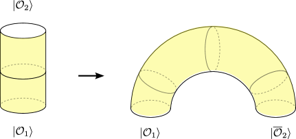
Figure 5: Two ways of computing the two point function and how to flip the operator $|{\mathcal{O}}_{2}\rangle$ to $|\bar{\mathcal{O}}_{2}\rangle$.

Due to the large degeneracy of trace states at tree level, one prefers to use a pre-diagonalization and use as basis of states the eigenstates of the one-loop dilatation operator, which is conveniently given by (nested) algebraic Bethe ansatz. Suppose that we have built the one-loop Lax matrix

$$L_{s}(u)=u-i/2-i(-1)^{|A|}E_{0}^{AB}E_{s}^{BA}\;.$$ (90)

where the generators in the auxiliary space $E_{0,d}^{AB}$ belong to the defining $(4|4$ dimensional) representation of $\mathfrak{psu}(2,2|4)$ and $E^{AB}_{s}$ are the generators in the actual physical representation, e.g. the oscillators representation. Using the property (88) of the vertex it is straightforward to show that

$$L^{(1)}(u)|{\cal V}_{12}\rangle=-L^{(2)}(-u)|{\cal V}_{12}\rangle\;.$$ (91)

Since the vertex carries the physical representation and its dual, one could interpret the above relation as the crossing relation. This point can be made more explicit by using the set of generators $\bar{E}^{AB}$ defined in (2) which act naturally in the dual representation. The change of sign in the Lax matrix can be absorbed in the normalization, and we will tacitly assume in the following that we have done so. Let us now consider the monodromy matrices of the two chains

$$T^{(1)}(u)=L_{1}^{(1)}(u)\ldots L_{L}^{(1)}(u)\;,\qquad T^{(2)}(u)=L_{L}^{(2)}(u)\ldots L_{1}^{(2)}(u)$$ (92)

and apply repeatedly the relation (91). We remind the convention (78) for the order of the sites of the second chain. The result is

$$L_{1}^{(1)}(u)\ldots L_{L}^{(1)}(u)|{\cal V}_{12}\rangle=L_{1}^{(2)}(-u)\ldots L_{L}^{(2)}(-u)|{\cal V}_{12}\rangle\;.$$ (93)

The right hand side is not exactly the monodromy matrix for the second chain $T^{(2)}(u)$, because the Lax matrices are in reverse order. This mismatch can be cured by taking an operation which reverses the order of the operators, like the (super) transposition ${}^{t_{0}}$ in the auxiliary space. In some sectors of $\mathfrak{psu}(2,2|4)$ one can correlate the change of the signs of the supertraceless generators $E^{ab}$ with the transposition

$$E^{ab}=-\sigma E^{ab,t}\sigma^{-1}\;.$$ (94)

where ^t denotes the (super) transposition in the quantum space. This is the case, for example, for the $\mathfrak{so}(4)\simeq\mathfrak{su}(2)_{L}\otimes\mathfrak{su}(2)_{R}$ sector, where $\sigma=\sigma^{-1}=-\sigma_{2,L}\sigma_{2,R}=U_{F}^{2}$. As one can check on (90), in any of the $\mathfrak{su}(2)$ sectors we have

$$L(u)=L^{t_{0},t}(u)=-\sigma L^{t_{0}}(-u)\sigma^{-1}=-\sigma_{0}L^{t_{0}}(-u)\sigma_{0}^{-1}\;,$$ (95)

where $\sigma_{0}=i\sigma_{2,0}$. The last equality sign comes from the invariance of the Lax matrix $[L_{s}(u),E^{ab}_{0}+E^{ab}_{s}]=0$. Substituting one of the last two equalities above into the r.h.s. of in (93) we obtain

$$T^{(1)}(u)|{\cal V}_{12}\rangle=\sigma\,T^{(2),t_{0}}(u)\sigma^{-1}|{\cal V}_{12}\rangle=\sigma_{0}T^{(2),t_{0}}(u)\sigma_{0}^{-1}|{\cal V}_{12}\rangle\;.$$ (96)

or in matrix form

$$\left(\begin{array}[]{cc}A(u)&B(u)\\ C(u)&D(u)\end{array}\right)^{\!\!\!(1)}\!\!\!|{\cal V}_{12}\rangle =\left(\begin{array}[]{cc}\sigma A(u)\sigma^{-1}&\sigma C(u)\sigma^{-1}\\ \sigma B(u)\sigma^{-1}&\sigma D(u)\sigma^{-1}\end{array}\right)^{\!\!\!(2)}|{\cal V}_{12}\rangle=\left(\begin{array}[]{cc}D(u)&-B(u)\\ -C(u)&A(u)\end{array}\right)^{\!\!\!(2)}\!\!\!|{\cal V}_{12}\rangle\;.$$ (103)

We will exemplify now the consequence of these relation in a given $\mathfrak{su}(2)$ sub-sector. The eigenvectors of the dilatation operator can be constructed by the action of the $B$ operators on the vacuum state $|Z^{L}\rangle$ followed by an arbitrary $\mathfrak{so}(6)$ rotation ${\cal R}$ in the quantum space,

$$|{\mathcal{O}}\rangle={\cal R}\;{B}(u_{1})\ldots{B}(u_{M})|Z^{L}\rangle\;.$$ (104)

The global rotation ${\cal R}$ changes the orientation of the $\mathfrak{su}(2)$ sector inside $\mathfrak{so}(6)$. Let us note that if we descend to $\mathfrak{so}(4)$, there are two different orbits the $\mathfrak{su}(2)$ sectors inside $\mathfrak{so}(4)$, called in the literature $\mathfrak{su}(2)_{R}$ and $\mathfrak{su}(2)_{L}$ and obtained by rotating $(Z,X)$ and $(Z,\bar{X}$) respectively. The two orbits are related to each other by improper rotations. Since we are working with operators which do not have components outside the $\mathfrak{so}(6)$ sector, we are going to use a version of the vertex $\langle v_{12}|$ truncated to $\mathfrak{so}(6)$. By equation (103) we obtain the rule which transfers the Bethe operators from one space to the other through the vertex,

$$\langle v_{12}|[{\cal R}\, B(u_{1})\ldots B(u_{M})]^{(1)}=\langle v_{12}|[B(u_{M})\ldots B(u_{1})\,{\cal R}^{-1}]^{(2)}$$

$$=\langle v_{12}|[\sigma\,C(u_{M})\ldots C(u_{1})\sigma{\cal R}^{-1}]^{(2)}\;.$$ (105)

This relation is fundamental in exploiting the vertex, and it prescribes in particular how to characterize the flipped states

$$\;{}^{(2)}\langle{\bar{\mathcal{O}}}|=\langle v_{12}|{\mathcal{O}}\rangle^{(1)}=$$ (106)

$$=\langle v_{12}|\;[B(u_{M})\ldots B(u_{1}) \,{\cal R}^{-1}]^{(2)}\;|Z^{L}\rangle^{(1)}=\,^{(2)}\langle\bar{Z}^{L}|\;[B(u_{M})\ldots B(u_{1})\,{\cal R}^{-1}]^{(2)}$$

$$=\langle v_{12}|\;[\sigma\,C(u_{M})\ldots C(u_{1})\,\sigma\,{\cal R}^{-1}]^{(2)}\;|Z^{L}\rangle^{(1)}=\,^{(2)}\langle Z^{L}|\;[C(u_{M})\ldots C(u_{1})\,\sigma\,{\cal R}^{-1}]^{(2)}$$

Using $B(u)^{\dagger}=-C(u^{*})$ and considering distributions of rapidities which are self-conjugate, $\{u\}=\{u^{*}\}$ we conclude that, up to an overall sign,

$$|\bar{\mathcal{O}}\rangle={\cal R}\,C(u_{1})\ldots C(u_{M})\,|\bar{Z}^{L}\rangle={\cal R}\,\sigma\,B(u_{1})\ldots B(u_{M})\,|Z^{L}\rangle\;.$$ (107)

Keeping in mind that $|\bar{\mathcal{O}}\rangle$ lives in a spin chain with the order of the site reversed with respect to $|{\mathcal{O}}\rangle$ we conclude that this is essentially the flipping procedure of EGSV . The alternative definitions of the Bethe vectors like in (107) can be used at will in order to express the overlaps in a convenient form. For example the last equality in the above equation can be proven to be equivalent to the result by one of the authors and Y. Matsuo SZ that the scalar product of one on-shell and one off-shell Bethe state are Izergin determinants.

3.2.2 Tree level correlation function in the $\mathfrak{so}(6)$ sector and the overlaps

As we have already seen in equation (62), the two point function at tree level in the $\mathfrak{so}(6)$ sector can be reduced to the computation of an overlap,

$$\langle{\mathcal{O}}_{1}(x){\mathcal{O}}_{2}(y)\rangle=\langle\bar{\mathcal{O}}_{1}|U^{2}e^{iL^{+}(y-x)}|{\mathcal{O}}_{2}\rangle=\frac{\langle\bar{\mathcal{O}}_{1}|{\mathcal{O}}_{2}\rangle}{(x-y)^{2\Delta_{1}}}=\frac{\langle v_{12}|{\mathcal{O}}_{1}\rangle\otimes|{\mathcal{O}}_{2}\rangle}{(x-y)^{2\Delta_{1}}}\;,$$ (108)

where again $\langle v_{12}|$ is the vertex $\langle{\cal V}_{12}|$ reduced to the $\mathfrak{so}(6)$ sector. The same is valid for the three point function at tree level,

$$\langle{\cal O}_{2}(x_{2}) {\cal O}_{3}(x_{3}){\cal O}_{1}(x_{1})\rangle=$$

$$=\langle V_{123}|\,{\rm U}_{(13)}^{2}\,{\rm U}_{(12)}^{2}{\rm U}_{(32)}^{2}\;e^{i[L^{+}_{(1)}x_{1}+L^{+}_{(2)}x_{2}+L^{+}_{(3)}x_{3}]}|{\mathcal{O}}_{2}\rangle\otimes|{\mathcal{O}}_{3}\rangle\otimes|{\cal O}_{1}\rangle$$

$$=\frac{\langle v_{123}|{\mathcal{O}}_{2}\rangle\otimes|{\mathcal{O}}_{3}\rangle\otimes|{\cal O}_{1}\rangle}{|x_{12}|^{\Delta_{12}}|x_{13}|^{\Delta_{13}}|x_{23}|^{\Delta_{23}}}\,,$$ (109)

where $\Delta_{ij}=\Delta_{i}+\Delta_{j}-\Delta_{k}$ with $\{i,j,k\}=\{1,2,3\}$. To obtain this relation we use that at tree order we can freely split the chain $(i)$ into two pieces $(ij)$ and $(ik)$ which connect with chains $(j)$ and $(k)$ respectively, and

$$L_{(i)}^{+}=L_{(ij)}^{+}+L_{(ik)}^{+}\;,\qquad\langle{\cal V}_{123}|[L_{(ij)}^{+}+L_{(ji)}^{+}]=0\;,$$ (110)

then we use the normal form (63) of the operators $U_{(ij)}^{2}$ to evaluate the averages over the bosonic oscillators. The separation of space-time dependence and the structure constant is possible in the sectors that do not contain bosonic oscillators. In sectors which contain bosonic oscillators, like $\mathfrak{sl}(2)$ and $\mathfrak{su}(1|1)$, one can have typically several tensor structures for the space-time dependence 2011arXiv1109.6321C ; Costa:2011mg . So, in the $\mathfrak{so}(6)$ sector we can reduce the structure constant to the overlap

$$C_{123}=\langle v_{123}|{\mathcal{O}}_{2}\rangle\otimes|{\mathcal{O}}_{3}\rangle\otimes|{\cal O}_{1}\rangle\;,$$ (111)

where we suppose that the states $|{\mathcal{O}}_{i}\rangle$ are normalized, ${\cal N}_{i}=\langle{\mathcal{O}}_{i}|{\mathcal{O}}_{i}\rangle=1$. If this is not the case, one has to divide out $\sqrt{{\cal N}_{1}{\cal N}_{2}{\cal N}_{3}}$.

We would like now to discuss more in detail the correlation functions of three operators in different $\mathfrak{su}(2)$ sectors, since they have been studied in detail in the literature 2012arXiv1212.6563K ; 2011JHEP09132G ; Sobko:SoV . As we have already mentioned, there are two different orbits of the $\mathfrak{su}(2)$ sectors under the global $\mathfrak{so}(4)$ rotations, and we will call them after the $\mathfrak{su}(2)_{R}$ and $\mathfrak{su}(2)_{L}$ defined below. We take the convention

$$|Z\rangle=|0\rangle\;,\qquad|\bar{Z}\rangle=c_{1}^{\dagger}d_{1}^{\dagger}c_{2}^{\dagger}d_{2}^{\dagger}|0\rangle\;,\qquad|X\rangle=c_{1}^{\dagger}d_{1}^{\dagger}|0\rangle\;,\qquad|\bar{X}\rangle=-c_{2}^{\dagger}d_{2}^{\dagger}|0\rangle\;.$$ (112)

and that the $L$ sector is generated by $c_{1},d_{1}$ and the $R$ sector by $c_{2},d_{2}$. Obviously, the generators in the two sectors commute, and the operators $X,\bar{X},Z,\bar{Z}$ can be seen as basis vectors in the bi-fundamental representation of $\mathfrak{su}(2)_{R}\otimes\mathfrak{su}(2)_{L}$,

$$|Z\rangle=|\!\uparrow\rangle_{L}\otimes|\!\uparrow\rangle_{R}\equiv|\!\uparrow\uparrow\rangle\;,\qquad|\bar{Z}\rangle=|\!\downarrow\rangle_{L}\otimes|\!\downarrow\rangle_{R}\equiv|\!\downarrow\downarrow\rangle\;,$$ (113)

$$|X\rangle=|\!\uparrow\rangle_{L}\otimes|\!\downarrow\rangle_{R}\equiv|\!\uparrow\downarrow\rangle\;,\qquad|\bar{X}\rangle=-|\!\downarrow\rangle_{L}\otimes|\!\uparrow\rangle_{R}\equiv-|\!\downarrow\uparrow\rangle\;.$$

The authors of ShotaNew call this representation the double spin, or double chain, representation, which can be traced back to Kazakov:2004qf. Together, the two $\mathfrak{su}(2)$ sectors generate an $\mathfrak{so}(4)$ sector. The vertex reduced to this sector is

$$|v_{12}\rangle^{\mathfrak{so}(4)}= |Z\rangle\otimes|\bar{Z}\rangle+|X\rangle\otimes|\bar{X}\rangle+|\bar{Z}\rangle\otimes|Z\rangle+|\bar{X}\rangle\otimes|X\rangle=|v_{12}\rangle^{\mathfrak{su}(2)_{L}}\otimes|v_{12}\rangle^{\mathfrak{su}(2)_{R}}\;,$$

$$|v_{12}\rangle^{\mathfrak{su}(2)_{L,R}}=|\!\uparrow\rangle_{L,R}\otimes|\!\downarrow\rangle_{L,R}-|\!\downarrow\rangle_{L,R}\otimes|\!\uparrow\rangle_{L,R}\;.$$ (114)

We can have two different cases:

$i)$ The $RRR$ case, when all the three operators are in the same sector, say $R$. In this case, the three operators can be chosen as

$$|{\cal O}_{1}\rangle ={\cal R}_{1}B_{R}(u_{1})\ldots B_{R}(u_{M_{1}})\,|Z^{L_{1}}\rangle\;,$$ (115)

$$|{\cal O}_{2}\rangle ={\cal R}_{2}\,\sigma\,B_{R}(v_{1})\ldots B_{R}(v_{M_{2}})\,|Z^{L_{2}}\rangle\;,$$

$$|{\cal O}_{3}\rangle ={\cal R}_{3}\,\sigma\,B_{R}(w_{1})\ldots B_{R}(w_{M_{3}})\,|Z^{L_{3}}\rangle\;.$$

The convention is such that ${\cal R}_{1}={\cal R}_{2}={\cal R}_{3}=1$ reduces to the extremal case. Although the explicit computation of the structure constants goes beyond the scope of this paper, we can note that this case does not seem to be computable in the generic case without cutting the states into pieces as prescribed by EGSV .

$ii)$ The $RRL$ case, when two operators, say ${\mathcal{O}}_{1}$ and ${\mathcal{O}}_{2}$, are in the sector $R$ and ${\mathcal{O}}_{3}$ is in the sector $L$. In this case we choose

$$|{\cal O}_{1}\rangle ={\cal R}_{1}B_{R}(u_{1})\ldots B_{R}(u_{M_{1}})\,|Z^{L_{1}}\rangle\;,$$ (116)

$$|{\cal O}_{2}\rangle ={\cal R}_{2}\,\sigma\,B_{R}(v_{1})\ldots B_{R}(v_{M_{2}})\,|Z^{L_{2}}\rangle\;,$$

$$|{\cal O}_{3}\rangle ={\cal R}_{3}\,B_{L}(w_{1})\ldots B_{L}(w_{M_{3}})\,|Z^{L_{3}}\rangle\;.$$

Again, our choice is such that ${\cal R}_{1}={\cal R}_{2}={\cal R}_{3}=1$ is the case originally considered by EGSV EGSV . In this case the left and right sector decouple

$$C^{EGSV}_{123}=\,^{\mathfrak{so}(4)} \langle v_{123}|\ B_{L}(w)\,|Z^{L_{3}}\rangle\;\otimes\;\sigma_{(2)}\,B_{R}(v)\,|Z^{L_{2}}\rangle\;\otimes\;B_{R}(u)\,|Z^{L_{1}}\rangle$$ (117)

$$=\,^{\mathfrak{so}(4)}\langle v_{123} |\ \sigma_{(32)}\,B_{L}(w)\,|Z^{L_{3}}\rangle\;\otimes\;\sigma_{(21)}\,B_{R}(v)\,|Z^{L_{2}}\rangle\;\otimes\;B_{R}(u)\,|Z^{L_{1}}\rangle\;.$$

$$={\rm SIMPLE}\times{\rm INVOLVED}$$ (118)

The SIMPLE part is given by the contribution of the $L$ sector,

$${\rm SIMPLE}=\,^{\mathfrak{su}(2)_{L}}\langle v_{123}|\ \sigma_{(32)L}\,B_{L}(w)\,|\uparrow^{L_{3}}\rangle\,\otimes \;\sigma_{(21)L}\,|\uparrow^{L_{2}}\rangle\otimes|\uparrow^{L_{1}}\rangle$$

$$=\langle\downarrow^{L_{3}}|\,\sigma_{(32)L}\,B_{L}(w)\,|\uparrow^{L_{3}}\rangle$$ (119)

while INVOLVED is given by the contribution of the $R$ sector

$${\rm INVOLVED} =\,^{\mathfrak{su}(2)_{R}}\langle v_{123}|\;\sigma_{(32)R}\,|\uparrow^{L_{3}}\rangle\otimes\,\sigma_{(21)R}\,B_{R}(v)\,|\uparrow^{L_{2}}\rangle\otimes B_{R}(u)\,|\uparrow^{L_{1}}\rangle$$

$$=\,^{\mathfrak{su}(2)_{R}}\langle v_{12}|\;\sigma_{(21)R}\ \langle\,\uparrow^{L_{23}}|\,B_{R}(v)\,|\uparrow^{L_{2}}\rangle\otimes\langle\,\downarrow^{L_{13}}|B_{R}(u)\,|\uparrow^{L_{1}}\rangle$$ (120)

Now one can use the properties of the Bethe states to show that

$$\langle\,\uparrow^{L_{23}}|\,B_{R}(v)\,|\,\uparrow^{L_{2}}\rangle=B_{R}(v)\,|\uparrow^{L_{21}}\rangle=\langle\,\downarrow^{L_{13}}|\,B_{R}(i/2)^{L_{13}}\,B_{R}(v)\,|\uparrow^{L_{1}}\rangle\;,$$ (121)

where the $L_{13}$ operators $B(i/2)$ are freezing $L_{13}$ consecutive sites to their $\downarrow$ value Omar . This implies also that freezing selects a single component from the vertex $\langle v_{13}|$

$$\,{}^{\mathfrak{su}(2)_{R}}\,\langle v_{13}|\,\sigma_{(13)R}\,B_{R}(i/2)^{L_{13}}\,B_{R}(v)\,|\uparrow^{L_{1}}\rangle=\langle\,\downarrow^{L_{13}}|\otimes\langle\,\downarrow^{L_{13}}|\,B_{R}(i/2)^{L_{13}}B_{R}(v)|\uparrow^{L_{1}}\rangle$$ (122)

we obtain finally

$${\rm INVOLVED} =\,^{\mathfrak{su}(2)_{R}}\langle v_{12}|\,\langle v_{13}|\,\sigma_{(1)R}\,B_{R}(i/2)^{L_{13}}B_{R}(v)\,|\uparrow^{L_{1}}\rangle\otimes B_{R}(u)\,|\uparrow^{L_{1}}\rangle\;.$$ (123)

So we have transformed the involved part into an overlap involving a single spin chain of length $L_{1}$. This is the result of EGSV EGSV combined with O. Foda’s freezing trick Omar . The case when the global rotations ${\cal R}_{1},\ {\cal R}_{2},\ {\cal R}_{3}$ are arbitrary is considered in ShotaNew .

3.3 Scalar products and global $\mathfrak{su}(2)$ rotations

Although considering correlators with the global $\mathfrak{so}(6)$ rotations goes beyond the scope of this work, it is relatively simple and instructive to consider the scalar product of two $\mathfrak{su}(2)$ Bethe states $|\{u\}\rangle$ and $|\{v\}\rangle$ that are rotated with respect to each other with an $\mathfrak{su}(2)$ rotation,

$${\cal R}_{\mathfrak{su}(2)}=e^{a\sigma^{+}}e^{ia_{3}\sigma_{3}}e^{-\bar{a}\sigma^{-}}\;.$$ (124)

By expanding the left and right factors in the rotation, $e^{a\sigma^{+}}=\sum_{k\geq 0}a^{k}(\sigma^{+})^{k}/k!$ and supposing that $\{u\}$ and $\{v\}$ contain the same number of mangons $M$, we get

$$\langle\{u\}|{\cal R}_{\mathfrak{su}(2)}|\{v\}\rangle=e^{ia_{3}(L-2M)}\sum_{k=0}^{L-2M}\frac{(-a\bar{a}e^{-2ia_{3}})^{k}}{(k!)^{2}}\langle\{u\};k|k;\{v\}\rangle\;,$$ (125)

with the state $|k;\{v\}\rangle$ containing $k$ magnons at infinity. The reason that the sum stops at $L-2M$, and not at $L-M$, as one could naively think, is that the state $|\{v\}\rangle$ is the highest weight state of a multiplet with spin $L/2-M$ and as such one cannot act on it more than $L-2M$ times with lowering operators. As shown in appendix B, if at least one of the states $|\{u\}\rangle$ and $|\{v\}\rangle$ is on-shell, the scalar products with $k$ magnons sent to infinity is given by

$$\langle\{u\};k|k;\{v\}\rangle=(k!)^{2}{L-2M\choose k}\langle\{u\}|\{v\}\rangle\;.$$ (126)

After resumming the sum in (125) one obtains the simple expression

$$\langle\{u\}|{\cal R}_{\mathfrak{su}(2)}|\{v\}\rangle=(e^{ia_{3}}-a\bar{a}e^{-ia_{3}})^{L-2M}\langle\{u\}|\{v\}\rangle\;.$$ (127)

It is interesting and reassuring to note that this relation holds when the scalar product $\langle\{u\}|\{v\}\rangle$ can be put in a determinant expression. It would be interesting to check whether this relation hold for more general rotations, for example in $\mathfrak{su}(3)$, where determinant expressions for states with some set of magnons at infinity also exist Wheeler-SU3 .

4 Monodromy condition on the spin vertex

In this section we are going to show that the local symmetry condition (88) of the spin vertex can be reformulated as an extended symmetry. This is the same Yangian symmetry, satisfied by the tree-level amplitudes in ${\cal N}=4$ SYM Drummond:Yangian .

The spin vertex is an invariant of the Yangian. We are going first to show this on the two-vertex, and then extend it to the three-vertex we need to compute the three point function. There are two types of monodromy matrices which are interesting for us. The first is the monodromy matrix where the auxiliary space is in the defining, $4|4$ dimensional, representation. This monodromy matrix is useful to build the Yangian generators and the for the nested Bethe ansatz procedure. The second type of monodromy matrix, useful for getting the local conserved quantities, contains the same physical representation in the auxiliary and quantum spaces. Here we construct the monodromy matrix with the auxiliary space in the defining representation. For the monodromy matrix with the auxiliary space in the physical representation, the construction of the $\mathfrak{so}(6)$ sector is relatively straightforward, however the construction in the $\mathfrak{sl}(2)$ sector is more subtle and we are not doing it here.

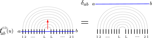
Figure 6: The two chain monodromy matrix $t^{(12)}(u)$ and its action on the vertex $|{\cal V}_{12}\rangle$

Let us take the $\mathfrak{psu}(2,2|4)$ $R$ matrix in the defining and physical representation

$$R_{01}(u)=u-i\Pi_{01}\;,\qquad\Pi_{01}=(-1)^{|A|}E_{0}^{AB}E_{1}^{BA}\;,$$ (128)

where $E_{0}^{AB}$ are $4|4\times 4|4$ super matrices and the generators in the quantum space are in the oscillator representation $E_{1}^{BA}=\bar{\psi}^{A}\psi^{B}$. When $E_{1}^{BA}$ are also in the defining representation, $\Pi_{01}$ is a super-permutation. In the representation we are considering

$$\Pi_{01}^{2} =(-1)^{|A|+|C|}E_{0}^{AB}E_{1}^{BA}E_{0}^{CD}E_{1}^{DC}=(-1)^{|A|+|B|+(|A|+|B|)(|B|+|D|)}E_{0}^{AD}E_{1}^{BA}E_{1}^{DB}$$ (129)

$$=(-1)^{|A|}E_{0}^{AD}E_{1}^{DA}(E_{1}^{BB}-1)+E_{1}^{BB}=\Pi_{01}(E_{1}^{BB}-1)+E_{1}^{BB}=-\Pi_{01}\;.$$

Here we have used the (anti)commutation relations $[\psi^{A},\bar{\psi}^{B}]_{\pm}=\delta^{AB}$ and that in the physical representation $c=E^{BB}_{1}=\bar{\psi}^{B}\psi^{B}=0$ and in the auxiliary representation $E_{0}^{BB}=1$. The $R$ matrix above satisfies the unitarity condition

$$R_{01}(u)R_{01}(-i-u)=-u(i+u)\;.$$ (130)

For a representation with arbitrary central charge $c$, the unitarity condition would be

$$R_{01}(u)R_{01}(i(c-1)-u)=-u(i(1-c)+u)-c\;.$$ (131)

We are now going to build the monodromy condition for the two-site vertex $|{\cal V}_{12}\rangle$,

$$R_{01}(u)R_{02}(u)|{\cal V}_{12}\rangle=-R_{01}(u)R_{01}(-i-u)|{\cal V}_{12}\rangle=u(u+i)|{\cal V}_{12}\rangle\;.$$ (132)

Here we have used that the $R$ matrix is related to the Lax matrix defined in (90) by $R_{01}^{(2)}(u)=L^{(2)}(u+i/2)$, and then use the crossing-like property (91) of the vertex

$$R_{02}(u)|{\cal V}_{12}\rangle=-R_{01}(-i-u)|{\cal V}_{12}\rangle.$$ (133)

The condition (132) can be lifted to the two-vertex with an arbitrary number of sites, as depicted in figure 6

$$T_{12}(u)=R^{(1)}_{01}(u)\ldots R^{(1)}_{0L}(u)\;R^{(2)}_{0L}(u)\ldots R^{(2)}_{01}(u)\;|{\cal V}_{12}\rangle=(u(u+i))^{L}|{\cal V}_{12}\rangle\;.$$ (134)

as well as for the three vertex, where the different pieces $t^{(ij)}(u)$ joining chain $(i)$ to chain $(j)$ are glued as in figure 4,

$$T_{123}(u)=t^{(12)}(u)t^{(13)}(u)t^{(31)}(u)t^{(32)}(u)t^{(23)}(u)t^{(21)}(u)\;.$$ (135)

The subsectors: The $\mathfrak{psu}(2,2|4)$ $R$ matrix can be readily reduced to different subsectors, just by restricting the sum in the definition of the central charge (25) to the corresponding subsector. As a result, the central charge can take non-zero value $c=E^{BB}_{1}$.

• In the $\mathfrak{su}(1|1)$, $\mathfrak{su}(2|3)$ and $\mathfrak{su}(2)$ sector, where the fields belong to the fundamental representation, $c=1$, so that the unitarity condition is slightly modified,

  $$\Pi_{01}^{2}=1\;,\qquad R_{01}(u)R_{01}(-u)=-(u^{2}+1)\;.$$ (136)

  The monodromy condition will be

  $$R_{01}(u)R_{02}(u-i)|{\cal V}_{12}\rangle=-R_{01}(u)R_{01}(-u)|{\cal V}_{12}\rangle=(u^{2}+1)|{\cal V}_{12}\rangle\;.$$ (137)

• In the $\mathfrak{sl}(2)$ sector, $c=0$, so the unitarity and monodromy conditions are the same as for $\mathfrak{psu}(2,2|4)$.

• In the $\mathfrak{so}(6)$ sector we have $c=2$, so that

  $$\Pi_{01}^{2}=\Pi_{01}+2\;,\qquad R_{01}(u)R_{01}(i-u)=u(i-u)-2\;.$$ (138)

  The monodromy condition is then

  $$R_{01}(u)R_{02}(u-2i)|{\cal V}_{12}\rangle=-R_{01}(u)R_{01}(i-u)|{\cal V}_{12}\rangle=(u(u-i)+2)|{\cal V}_{12}\rangle\;.$$ (139)

5 Conclusion and Outlook

In this paper we proposed a new formulation for computing correlation functions in planar $\mathcal{N}=4$ SYM theory. In this novel formalism, the central object is called the spin vertex, which is the weak-coupling counter-part of the string vertex in the string field theory. We constructed the spin vertex for all sectors of the theory at tree-level by a set of bosonic and fermionic oscillators. The spin vertex is a special entangled state living in Hilbert space of multi spin chains and has many nice properties. In the spin vertex formalism, the symmetry of correlation functions become manifest. In particular, we are able to construct monodromy matrices under the action of which the spin vertex is invariant. In another word, the spin vertex is invariant under the action of the infinite dimensional Yangian algebra, which is the hallmark of integrability.

The spin vertex and its Yangian invariance is not only important conceptually, but is also very useful practically. Using the properties of spin vertex in an ingenious way, the authors of Shota1:Yangian were able to compute more general configurations of three-point functions both in the compact $SU(2)$ as well as in the non-compact $SL(2)$ Shota2 sectors in terms of determinants. In the semiclassical limit, the Yangian invariance of spin vertex is equivalent to the monodromy condition which plays an important role in the computation of three-points in the strong coupling limit Komatsu:3pt1 ; Komatsu:3pt2 ; Komatsu:su2 . This opens a new way of computing semi-classical three-point functions by similar techniques from strong coupling without using determinant formulas ShotaNew .

There are many open questions. First and foremost, the present work is inspired by the structure of the light-cone string field theory for strings moving on the pp-wave background. A natural question is whether we can recover the light-cone string field theory in the BMN limit. The BMN limit is a degenerate limit of AdS/CFT correspondence where all scattering phases are zero and hence integrability becomes trivial. However, it is interesting at both strong and weak coupling to see how this limit is achieved. This will be helpful to understand the BMN limit better and might shed some light on finite coupling regime. At the leading order, we can show that the spin vertex in the BMN limit reproduces exactly the structure of light-cone string field theory with the same Neumann coefficients. The derivation uses a polynomial representation of the spin vertex and the result will be presented elsewhere Jiang:Vertex .

Another important question is understanding how to deform the spin vertex and the corresponding Yangian invariance at higher loop orders in perturbation theory. In the computation of structure constants at loop orders, quantum corrections manifest themselves as operator insertions at the splitting points GV:quantumintegrability ; GV ; JKLS-fixing ; Pedro:sl23pt ; Caetano:Fermionic . At present, these operator insertions are computed by Feynmann diagrams which are usually rather complicated. The generalization for larger sectors and to higher loops in this way will be impractical. However, since the theory is integrable, it should be possible to fix these insertions from integrability, as in the case of the spectral problem. The higher loop deformation of the spin vertex should contain the operator insertions at higher loops. This problem is more subtle due to renormalization. In contrast to the tree-level, it is a non-trivial task to extract the renormalization scheme independent structure constant from the three-point function. However, we think that some general principles can still be applied. We expect that at higher loop the expression of the three point function is still given by

$$\langle{\cal O}_{2}(y){\cal O}_{2}(y){\cal O}_{1}(x)\rangle=\langle{\cal V}_{123}|\,e^{i(L^{+}_{1}x+L^{+}_{2}y+L^{+}_{3}z)}|{\mathcal{O}}_{2}\rangle\otimes|{\mathcal{O}}_{3}\rangle\otimes|{\cal O}_{1}\rangle\,,$$ (140)

with all the quantities receiving radiative corrections. The space-time dependence of the correlator can be fixed by using Ward identities, that can be derived for example by inserting the energy operator $E_{1}+E_{2}+E_{3}$. The constraints that the vertex has to satisfy at any loop order is

$$(E_{1}+E_{2}+E_{3})|{\cal V}_{123}\rangle=0\,.$$ (141)

A similar constraint can be derived from the monodromy relation (135). This suggests that the infinite Yangian symmetry could be translated into Ward identities which would determine the three-point correlation function. We hope to be able to report on this in the near future.

Finally, we would like to point out the similarity between our construction of the spin vertex and the scattering amplitudes. Yangian invariants were recently exploited to build the scattering amplitudes Ferro:2012xw ; Chicherin-Kirchner ; Chicherin ; Frassek2013 ; Florian-ampl ; Staudacher:Yangian ; Kanning:2014maa . Their key point is to regard the scattering amplitudes as Yangian invariants and try to construct it explicitly from Bethe ansatz. To certain extent, the spin vertex constructed in this paper is the simplest possible Yangian invariant one can construct. It is interesting to understand whether more general Yangian invariants will play some role in the construction of spin vertex, especially at higher loops. In both cases, the understanding of how to deform Yangian invariants at higher loops is crucial. This observation shows that Yangian invariant may be the key to understand both on-shell quantities like scattering amplitudes and off-shell quantities like correlation functions. It will be fascinating to develop a common framework and have a unified description of these two kinds of quantities.

Appendix A The operator ${\rm U}$

In this Appendix we collect some formulas about the action of the operator ${\rm U}=UU_{F}$ which represents a finite super-conformal transformation. The operator is a product of a $\mathfrak{su}(2,2)$-rotation in imaginary angle

$$U=e^{-\frac{\pi}{4}(P_{0}-K_{0})}=e^{-\frac{\pi}{4}(L^{+}_{0}-L^{-}_{0})}=e^{-\frac{\pi}{4}(a_{i}^{\dagger}b_{i}^{\dagger}+b_{i}a_{i})}\;$$ (142)

and a unitary $\mathfrak{su}(4)$-rotation

$$U_{F}=e^{-{\pi\over 4}(R_{13}-R_{31}+R_{24}-R_{42})}=e^{-\frac{\pi}{4}(c_{i}^{\dagger}d_{i}^{\dagger}-d_{i}c_{i})}\;.$$ (143)

As it was suggested in ADGN , it is convenient to first to compute the action of a rotation in an arbitrary angle $it$

$$U_{t}=U_{t}^{\dagger}\equiv e^{t(a_{i}^{\dagger}b_{i}^{\dagger}+b_{i}a_{i})}.$$ (144)

The action of $U_{t}$ on the oscillators $a_{i},a^{\dagger}_{i},b_{i},b^{\dagger}_{i}$ is

$$a_{i}(t)\equiv U_{t}a_{i}U_{t}^{-1}=a_{i}\cos t-b_{i}^{\dagger}\sin t,\quad b_{i}(t)\equiv U_{t}b_{i}U_{t}^{-1}=b_{i}\cos t-a_{i}^{\dagger}\sin t,$$

$$a^{\dagger}_{i}(t)\equiv U_{t}a^{\dagger}_{i}U_{t}^{-1}=a_{i}^{\dagger}\cos t+b_{i}\sin t,\quad b^{\dagger}_{i}(t)\equiv U_{t}b^{\dagger}_{i}U_{t}^{-1}=b_{i}^{\dagger}\cos t+a_{i}\sin t.$$ (145)

From here one easily obtains the normal form of the operator $U_{t}$ is ADGN

$$U_{t}\equiv e^{t\left(a^{\dagger}b^{\dagger}+ba\right)} = {1\over\cos^{2}t}\ e^{\tan t\,a^{\dagger}b^{\dagger}}(\cos t)^{-\,a_{i}^{\dagger}a-b^{\dagger}_{i}b}\ e^{\tan t\,ba},$$ (146)

or, in terms of the Lie-algebra generators,

$$U_{t}=e^{-t(L^{+}_{0}-L^{-}_{0})}={1\over\cos^{2}t}\epsilon^{-L^{+}_{0}\tan t}\cos(t)^{-2E}e^{L_{0}^{-}\tan t}.$$ (147)

Similarly one derives the normal form of the compact piece (45) by introducing the rotation at angle $t$,

$$U_{t}^{F}\equiv e^{t\left(c^{\dagger}d^{\dagger}+cd\right)} = {\cos^{2}t}\ e^{\tan t\,c^{\dagger}d^{\dagger}}(\cos t)^{-\,c_{i}^{\dagger}c_{i}-d^{\dagger}_{i}d}\ e^{\tan t\,cd}.$$ (148)

In the normal form of the full operator, the $\cos t$ factors nicely cancel,

$${\rm U}_{t} \equiv e^{t\left(a^{\dagger}b^{\dagger}+ab+c^{\dagger}d^{\dagger}+cd\right)}$$ (149)

$$= e^{\tan t\,(a^{\dagger}b^{\dagger}+c^{\dagger}d^{\dagger})}e^{-\log\cos t(a^{\dagger}a+b^{\dagger}b+c^{\dagger}c+d^{\dagger}d}e^{\tan t\,(ab+cd)}.$$

From (149) one obtains the regularised expression for the conjugate vacuum $|\bar{0}\rangle=|\bar{0}\rangle_{B}\otimes|\bar{0}\rangle_{F}$,

$$|\bar{0}\rangle\equiv{\rm U}^{2}|0\rangle \approx e^{(a^{\dagger}b^{\dagger}+c^{\dagger}d^{\dagger})/\epsilon}|0\rangle$$ (150)

$$\approx {e^{a^{\dagger}b^{\dagger}/\epsilon}\over\epsilon^{2}}\ c^{\dagger}_{1}c^{\dagger}_{2}\ d^{\dagger}_{2}d^{\dagger}_{1}|0\rangle\,,\qquad\epsilon\to 0.$$

Appendix B Sending roots to infinity

The limit $u\to\infty$ is delicate and can produce different results. Here it is important that half of the roots are on shell and that we send to infinity $k$ on-shell roots and $k$ off-shell roots. We proceed as follows: first send sequentially $k$ on-shell ${{\{u\}}}$-roots to infinity so that the Bethe equations are satisfied in the process. This is important, because otherwise the scalar product is not given by a determinant. Then we send $k$ off-shell ${\{v\}}$-roots to infinity.

Proceeding as in SL (eq. (3.24)) and taking into account that $f(v_{j})\approx e^{iG_{{\{u\}}}+iG_{\{v\}}-L/u}\approx e^{i(2N-L)/v_{j}}$ for the $v$-roots, and as $f(u_{k})\approx e^{iG_{\{v\}}-iG_{{\{u\}}}}\approx e^{0/u_{k}}$ because of the Bethe equations, one obtains the general formula, when $K^{\prime}=N-M^{\prime}$ roots ${{\{u\}}}$ (on shell) and $K^{\prime\prime}=N-M^{\prime\prime}$ roots ${\{v\}}$ (off shell) are sent to infinity:

$$\lim_{v_{N-K+1},\dots,v_{N}\to\infty}\left[\left(\prod_{j=M^{\prime\prime}+1}^{N}v_{j}\right)\lim_{u_{N-K+1},\dots,u_{N}\to\infty}\left(\prod_{j=M^{\prime}+1}^{N}u_{j}\right)\langle{{\{u\}}}_{N}|{\{v\}}_{N}\rangle\right]$$

$$=(N-M^{\prime})!(N-M^{\prime\prime})!\begin{pmatrix}L-M^{\prime}-M^{\prime\prime}\\ N-M^{\prime\prime}\end{pmatrix}{\mathcal{A}}_{{{\{u\}}}_{M^{\prime}}\cup{\{v\}}_{M^{\prime\prime}}}.$$ (151)

where ${\mathcal{A}}_{{{\{u\}}}_{M^{\prime}}\cup{\{v\}}_{M^{\prime\prime}}}$ is the determinant expression giving the scalar product SL . Taking $K^{\prime}=K^{\prime\prime}=k$ one obtains the correct combinatorial factor from equation (126)

$$\langle{{\{u\}}};k|k;{\{v\}}\rangle=(k!)^{2}{L-2M\choose k}\langle{{\{u\}}}|{\{v\}}\rangle\;.$$ (152)

Appendix C The Spin Vertex as a Flipping Operator

In section we will justify the expression for the spin vertex (3.1) and explain why the expressions (7), (8) give the correct expression for the two- and three-point functions.

The propagators for the elementary fields have the following form:

$$\begin{split}&\langle\bar{S}(y){S}(x)\rangle=\frac{1}{(x-y)^{2}},\quad S=X,Y,Z,\\ &\langle\bar{\Psi}_{jb}(y){\Psi}_{ia}(x)\rangle=i\delta_{ab}\sigma_{ij}^{\mu}\partial_{x^{\mu}}\frac{1}{(x-y)^{2}},\quad a,b=1,...,4,\quad i,j=1,2,\\ &\langle{\cal F}_{\rho\sigma}(y){\cal F}_{\mu\nu}(x)\rangle=(\eta_{\nu\sigma}\partial_{\mu}\partial_{\rho}+\eta_{\mu\rho}\partial_{\nu}\partial_{\sigma}-\eta_{\mu\sigma}\partial_{\nu}\partial_{\rho}-\eta_{\nu\rho}\partial_{\mu}\partial_{\sigma})\frac{1}{(x-y)^{2}}.\end{split}$$ (153)

We have to show that the spin vertex formalism reproduce these propagators correctly, by means of the equation

$$\langle{\cal O}_{2}(y){\cal O}_{1}(x)\rangle=\langle{\cal V}_{12}|\,e^{i(L^{+}_{1}x+L^{+}_{2}y)}|{\mathcal{O}}_{2}\rangle\otimes|{\cal O}_{1}\rangle\,.$$ (154)

First we establish the rule how the vertex transform the fields form the space $(2)$ to the space $(1)$. Using the representation of the elementary fields in terms of the oscillators

$$\begin{split}&Z=|0\rangle,\quad\bar{Z}=c_{1}^{\dagger}d_{1}^{\dagger}c_{2}^{\dagger}d_{2}^{\dagger}|0\rangle,\\ &Y=c_{2}^{\dagger}d_{1}^{\dagger}|0\rangle,\quad\bar{Y}=c_{1}^{\dagger}d_{2}^{\dagger}|0\rangle,\\ &X=c_{1}^{\dagger}d_{1}^{\dagger}|0\rangle,\quad\bar{X}=-c_{2}^{\dagger}d_{2}^{\dagger}|0\rangle,\\ &\Psi_{i1}=b_{i}^{\dagger}c_{2}^{\dagger}|0\rangle,\quad\bar{\Psi}_{i1}=-a_{i}^{\dagger}c_{1}^{\dagger}d_{2}^{\dagger}d_{1}^{\dagger}|0\rangle,\\ &\Psi_{i2}=-b_{i}^{\dagger}c_{1}^{\dagger}|0\rangle,\quad\bar{\Psi}_{i2}=-a_{i}^{\dagger}c_{2}^{\dagger}d_{2}^{\dagger}d_{1}^{\dagger}|0\rangle,\\ &\Psi_{i3}=b_{i}^{\dagger}c_{1}^{\dagger}c_{2}^{\dagger}d_{1}^{\dagger}|0\rangle,\quad\bar{\Psi}_{i3}=a_{i}^{\dagger}d_{2}^{\dagger}|0\rangle,\\ &\Psi_{i4}=b_{i}^{\dagger}c_{1}^{\dagger}c_{2}^{\dagger}d_{2}^{\dagger}|0\rangle,\quad\bar{\Psi}_{i4}=-a_{i}^{\dagger}d_{1}^{\dagger}|0\rangle,\\ &{F}_{ij}=-b_{i}^{\dagger}b_{j}^{\dagger}c_{1}^{\dagger}c_{2}^{\dagger}|0\rangle,\quad\bar{F}_{ij}=a_{i}^{\dagger}a_{j}^{\dagger}d_{1}^{\dagger}d_{2}^{\dagger}|0\rangle,\end{split}$$ (155)

we obtain by by direct computation

$$\begin{split}&{}^{(2)}\langle S|U_{F}^{2}|V_{12}\rangle=|\bar{S}\rangle^{(1)},\quad{}^{(2)}\langle\bar{S}|U_{F}^{2}|V_{12}\rangle=|S\rangle^{(1)},\quad S=X,Y,Z\\ &{}^{(2)}\langle\Psi_{ia}|U_{F}^{2}|V_{12}\rangle=|\bar{\Psi}_{ia}\rangle^{(1)},\quad{}^{(2)}\langle\bar{\Psi}_{ia}|U_{F}^{2}|V_{12}\rangle=|\Psi_{ia}\rangle^{(1)},\\ &{}^{(2)}\langle F_{ij}|U_{F}^{2}|V_{12}\rangle=|\bar{F}_{ij}\rangle^{(1)},\quad{}^{(2)}\langle\bar{F}_{ij}|U_{F}^{2}|V_{12}\rangle=|F_{ij}\rangle^{(1)},\\ \end{split}$$ (156)

where

$$\begin{split}&U_{F}^{2}|V_{12}\rangle=e^{\sum\limits_{i=1,2}(b_{i}^{(1)\dagger}a_{i}^{(2)\dagger}-a_{i}^{(1)\dagger}b_{i}^{(2)\dagger}+c_{i}^{(1)}c_{i}^{(2)\dagger}-d_{i}^{(1)}d_{i}^{(2)\dagger})}c_{1}^{(1)\dagger}d_{1}^{(1)\dagger}c_{2}^{(1)\dagger}d_{2}^{(1)\dagger}|0\rangle^{(1)}|0\rangle^{(2)},\end{split}$$ (157)

and

$$\begin{split}{\cal F}^{\mu\nu}=(\bar{\sigma}^{\mu\nu}\epsilon)_{ij}\bar{F}_{ij}-(\epsilon\sigma^{\mu\nu})_{ij}F_{ij},&\quad i,j=1,2,\quad\mu,\nu=1,...,4,\\ \sigma^{\mu\nu}=\frac{1}{4}\Big{(}\sigma^{\mu}\bar{\sigma}^{\nu}-\sigma^{\nu}\bar{\sigma}^{\mu}\Big{)},&\quad\bar{\sigma}^{\mu\nu}=\frac{1}{4}\Big{(}\bar{\sigma}^{\mu}\sigma^{\nu}-\bar{\sigma}^{\nu}\sigma^{\mu}\Big{)},\quad\epsilon_{12}=1.\end{split}$$ (158)

This leads to the following expansion for the vertex

$$U^{2}_{F}|V_{12}\rangle=|\bar{S}^{(2)}_{i}\rangle|S_{i}^{(1)}\rangle+|S^{(2)}_{i}\rangle|\bar{S}^{(1)}_{i}\rangle+|\bar{\Psi}^{(2)}_{ia}\rangle|\Psi^{(1)}_{ia}\rangle+|\Psi^{(2)}_{ia}\rangle|\bar{\Psi}^{(1)}_{ia}\rangle+|\bar{F}^{(2)}_{ij}\rangle|F^{(1)}_{ij}\rangle+|F^{(2)}_{ij}\rangle|\bar{F}^{(1)}_{ij}\rangle+...,$$ (159)

where we assume summation over repeating indexes and three dots mean other possible states appearing in the vertex expansion, including those not satisfying the zero central charge condition.

Now we are ready to compute the propagators using the (154). We start with the scalars.

$$\begin{split}&\langle\bar{S}(y){S}(x)\rangle=\langle{\cal V}_{12}|e^{i(L^{+}_{(1)}x+L^{+}_{(2)}y)}|\bar{S}\rangle_{(2)}\otimes|{S}\rangle_{(1)}=\langle{\cal V}_{12}|e^{i(L^{+}_{(1)}x-L^{+}_{(1)}y)}|\bar{S}\rangle_{(2)}\otimes|{S}\rangle_{(1)}=\\ &\langle V_{12}|U_{F(1)}^{2}U_{(1)}^{2}e^{i(L^{+}_{(1)}x-L^{+}_{(1)}y)}|\bar{S}\rangle_{(2)}\otimes|{S}\rangle_{(1)}=\langle S|U^{2}e^{i(L^{+}x-L^{+}y)}|S\rangle=\\ &\langle 0|U^{2}e^{i(L^{+}x-L^{+}y)}|0\rangle=\frac{1}{(x-y)^{2}},\end{split}$$ (160)

where in order to get the last line we used (62). For the fermions we’ll consider one of the possible propagators, the rest can be computed absolutely analogously:

$$\begin{split}&\langle\bar{\Psi}_{j4}(y){\Psi}_{i4}(x)\rangle=-\langle{\cal V}_{12}|e^{i(L^{+}_{(1)}x+L^{+}_{(2)}y)}a_{j}^{(2)\dagger}d_{1}^{(2)\dagger}|0\rangle_{(2)}b_{i}^{(1)\dagger}c_{1}^{(1)\dagger}c_{2}^{(1)\dagger}d_{2}^{(1)\dagger}|0\rangle_{(1)}=\\ &\langle 0|b_{i}d_{2}c_{2}c_{1}U^{2}e^{i(L^{+}x-L^{+}y)}b_{i}^{\dagger}c_{1}^{\dagger}c_{2}^{\dagger}d_{2}^{\dagger}|0\rangle=-\langle 0|U^{2}e^{-iL^{+}y}a_{j}^{\dagger}b_{i}^{\dagger}e^{iL^{+}x}|0\rangle=\frac{i}{2}\partial_{\mu}\sigma^{\mu}_{ij}\langle 0|U^{2}e^{i(L^{+}x-L^{+}y)}|0\rangle\\ &=\frac{i}{2}\partial_{\mu}\sigma^{\mu}_{ij}\frac{1}{(x-y)^{2}},\end{split}$$ (161)

where we used the explicit expression in terms of the oscillators for the $L^{+\mu}=-a_{i}^{\dagger}\bar{\sigma}_{ij}^{\mu}b_{j}^{\dagger}$ and the property of the $\sigma$ matrices

$$\sigma_{ij}^{\mu}(\bar{\sigma}_{\mu})_{kl}=-2\delta_{il}\delta_{jk}.$$ (162)

Finally we compute the propagator for the strength field:

$$\begin{split}&\langle F^{\rho\sigma}(y)F^{\mu\nu}(x)\rangle=\langle{\cal V}_{12}|e^{iL^{+}_{(1)}x}e^{iL^{+}_{(2)}y}\Big{(}(\bar{\sigma}^{\mu\nu}\epsilon)_{ij}a_{i}^{(2)\dagger}a_{j}^{(2)\dagger}d_{1}^{(2)\dagger}d_{2}^{(2)\dagger}+(\sigma^{\mu\nu})_{ij}b_{i}^{(2)\dagger}b_{j}^{(2)\dagger}c_{1}^{(2)\dagger}c_{2}^{(2)\dagger}\Big{)}|0\rangle_{(2)}\otimes\\ &\Big{(}(\bar{\sigma}^{\mu\nu}\epsilon)_{ij}a_{i}^{(1)\dagger}a_{j}^{(1)\dagger}d_{1}^{(1)\dagger}d_{2}^{(1)\dagger}+(\sigma^{\mu\nu})_{ij}b_{i}^{(1)\dagger}b_{j}^{(1)\dagger}c_{1}^{(1)\dagger}c_{2}^{(1)\dagger}\Big{)}|0\rangle_{(1)}=\\ &-(\bar{\sigma}^{\mu\nu}\epsilon)_{ij}(\epsilon\sigma^{\rho\sigma})_{kl}\langle 0|U^{2}e^{-iL^{+}y}a_{i}^{\dagger}a_{j}^{\dagger}b_{k}^{\dagger}b_{l}^{\dagger}e^{iL^{+}_{(1)}x}|0\rangle+(\mu\leftrightarrow\rho,\nu\leftrightarrow\sigma)=\\ &\frac{1}{4}(\bar{\sigma}^{\mu\nu}\epsilon)_{ij}(\epsilon\sigma^{\rho\sigma})_{kl}\sigma^{\kappa}_{ki}\sigma^{\omega}_{lj}\partial_{\kappa}\partial_{\omega}\frac{1}{(x-y)^{2}}+(\mu\leftrightarrow\rho,\nu\leftrightarrow\sigma)=\\ &\frac{1}{8}(\bar{\sigma}^{\mu\nu}\epsilon)_{ij}(\epsilon\sigma^{\rho\sigma})_{kl}\Big{(}\sigma^{\omega}_{lj}\sigma^{\kappa}_{ki}+\sigma^{\kappa}_{lj}\sigma^{\omega}_{ki}\Big{)}\partial_{\kappa}\partial_{\omega}\frac{1}{(x-y)^{2}}+(\mu\leftrightarrow\rho,\nu\leftrightarrow\sigma).\\ \end{split}$$ (163)

Further we use the following identity:

$$\sigma_{ij}^{\mu}\sigma_{kl}^{\nu}+(\mu\leftrightarrow\nu)=-\eta^{\mu\nu}\bar{\epsilon}_{ik}\bar{\epsilon}_{jl}+4\eta_{\kappa\omega}(\sigma^{\kappa\mu}\bar{\epsilon})_{ik}(\bar{\epsilon}\bar{\sigma}^{\omega\nu})_{jl},$$ (164)

where $\bar{\epsilon}_{12}=-1$. It gives

$$\begin{split}&\frac{1}{8}(\bar{\sigma}^{\mu\nu}\epsilon)_{ij}(\epsilon\sigma^{\rho\sigma})_{kl}\Big{(}-\eta^{\kappa\omega}\bar{\epsilon}_{lk}\bar{\epsilon}_{ji}+4\eta_{\tau\theta}(\sigma^{\tau\kappa}\bar{\epsilon})_{lk}(\bar{\epsilon}\bar{\sigma}^{\theta\omega})_{ji}\Big{)}\partial_{\kappa}\partial_{\omega}\frac{1}{(x-y)^{2}}+(\mu\leftrightarrow\rho,\nu\leftrightarrow\sigma)=\\ &\Big{(}-\frac{\eta^{\kappa\omega}}{8}{\rm Tr}(\sigma^{\rho\sigma}){\rm Tr}(\bar{\sigma}^{\mu\nu})+\frac{\eta_{\tau\theta}}{2}{\rm Tr}(\sigma^{\rho\sigma}\sigma^{\tau\kappa}){\rm Tr}(\bar{\sigma}^{\mu\nu}\bar{\sigma}^{\theta\omega})\Big{)}\partial_{\kappa}\partial_{\omega}\frac{1}{(x-y)^{2}}+(\mu\leftrightarrow\rho,\nu\leftrightarrow\sigma).\\ \end{split}$$ (165)

Next, noticing that ${\rm Tr}(\sigma^{\mu\nu})={\rm Tr}(\bar{\sigma}^{\mu\nu})=0$ and also using the relations

$$\begin{split}&{\rm Tr}(\sigma^{\mu\nu}\sigma^{\rho\sigma})=-\frac{1}{2}\Big{(}\eta^{\mu\rho}\eta^{\nu\sigma}-\eta^{\mu\sigma}\eta^{\nu\rho}+i\epsilon^{\mu\nu\rho\sigma}\Big{)},\\ &{\rm Tr}(\bar{\sigma}^{\mu\nu}\bar{\sigma}^{\rho\sigma})=-\frac{1}{2}\Big{(}\eta^{\mu\rho}\eta^{\nu\sigma}-\eta^{\mu\sigma}\eta^{\nu\rho}-i\epsilon^{\mu\nu\rho\sigma}\Big{)},\end{split}$$ (166)

we get

$$\begin{split}&\langle F^{\rho\sigma}(y)F^{\mu\nu}(x)\rangle=\frac{\eta_{\tau\theta}}{8}\Big{(}\eta^{\rho\tau}\eta^{\sigma\kappa}-\eta^{\rho\kappa}\eta^{\tau\sigma}+i\epsilon^{\rho\sigma\tau\kappa}\Big{)}\Big{(}\eta^{\mu\theta}\eta^{\nu\omega}-\eta^{\mu\omega}\eta^{\nu\theta}-i\epsilon^{\mu\nu\theta\omega}\Big{)}\partial_{\kappa}\partial_{\omega}\frac{1}{(x-y)^{2}}+\\ &(\mu\leftrightarrow\rho,\nu\leftrightarrow\sigma)=\frac{1}{8}\Big{(}\eta^{\sigma\kappa}\eta^{\mu\rho}\eta^{\nu\omega}-\eta^{\rho\nu}\eta^{\sigma\kappa}\eta^{\mu\omega}-\eta^{\rho\kappa}\eta^{\mu\sigma}\eta^{\nu\omega}+\eta^{\rho\kappa}\eta^{\mu\omega}\eta^{\nu\sigma}+i\epsilon^{\rho\sigma\mu\kappa}\eta^{\nu\omega}-i\epsilon^{\rho\sigma\nu\kappa}\eta^{\mu\omega}-\\ &i\epsilon^{\mu\nu\rho\omega}\eta^{\sigma\kappa}+i\epsilon^{\mu\nu\sigma\omega}\eta^{\rho\kappa}+\eta_{\tau\theta}\epsilon^{\rho\sigma\tau\kappa}\epsilon^{\mu\nu\theta\omega}\Big{)}\partial_{\kappa}\partial_{\omega}\frac{1}{(x-y)^{2}}+(\mu\leftrightarrow\rho,\nu\leftrightarrow\sigma).\\ \end{split}$$ (167)

One can see that after taking into account symmetrization with respect to the permutation $(\mu\leftrightarrow\rho,\nu\leftrightarrow\sigma)$ and also $(\kappa\leftrightarrow\omega)$, all the terms proportional to $i$ cancel out. Decomposition of the Levi-Civita tensor contraction gives (we use convention $\epsilon^{0123}=1$)

$$\eta_{\tau\theta}\epsilon^{\rho\sigma\tau\kappa}\epsilon^{\mu\nu\theta\omega}=\eta^{\sigma\nu}\eta^{\rho\omega}\eta^{\kappa\mu}+\eta^{\sigma\omega}\eta^{\rho\mu}\eta^{\kappa\nu}+\eta^{\rho\nu}\eta^{\sigma\mu}\eta^{\kappa\omega}-\eta^{\sigma\omega}\eta^{\rho\nu}\eta^{\kappa\mu}-\eta^{\sigma\mu}\eta^{\rho\omega}\eta^{\kappa\nu}-\eta^{\rho\mu}\eta^{\sigma\nu}\eta^{\kappa\omega}.$$ (168)

The terms proportional to $\eta^{\kappa\omega}$ cancel out due to equation of motion $\partial^{2}\frac{1}{(x-y)^{2}}=0$. Taking all this remarks into account we get final result:

$$\langle F^{\rho\sigma}(y)F^{\mu\nu}(x)\rangle=\frac{1}{2}\Big{(}\eta^{\sigma\kappa}\eta^{\mu\rho}\eta^{\nu\omega}-\eta^{\rho\nu}\eta^{\sigma\kappa}\eta^{\mu\omega}-\eta^{\rho\kappa}\eta^{\mu\sigma}\eta^{\nu\omega}+\eta^{\rho\kappa}\eta^{\mu\omega}\eta^{\nu\sigma}\Big{)}\partial_{\kappa}\partial_{\omega}\frac{1}{(x-y)^{2}}.$$ (169)

The action of covariant derivatives in terms of oscillators is given by ${\cal D}_{ij}=a^{\dagger}_{i}b^{\dagger}_{j}$. Thus, in case, when an elementary field belongs to the non-compact sector, the corresponding propagator can be obtained by taking appropriate number of derivatives contracted with right component of the sigma matrices, e.g.

$$\begin{split}&\langle\bar{Z}(y){\cal D}_{ij}Z(x)\rangle=\langle{\cal V}_{12}|e^{i(L^{+}_{(1)}x+L^{+}_{(2)}y)}|\bar{Z}\rangle_{(2)}\otimes|{\cal D}_{ij}Z\rangle_{(1)}\\ &=-\frac{i}{2}\sigma^{\mu}_{ji}\partial_{x^{\mu}}\langle{\cal V}_{12}|e^{i(L^{+}_{(1)}x+L^{+}_{(2)}y)}|\bar{Z}\rangle_{(2)}\otimes|Z\rangle_{(1)}=-\frac{i}{2}\sigma^{\mu}_{ji}\partial_{x^{\mu}}\frac{1}{(x-y)^{2}}.\end{split}$$ (170)

References

- (1) G. t Hooft, “A planar diagram theory for strong interactions,” Nuclear Physics B 72 (1974) 461–473.
- (2) J. M. Maldacena, “The large N limit of superconformal field theories and supergravity,” Adv. Theor. Math. Phys. 2 (1998) 231–252, hep-th/9711200.
- (3) S. S. Gubser, I. R. Klebanov, and A. M. Polyakov, “Gauge theory correlators from non-critical string theory,” Phys. Lett. B428 (1998) 105–114, hep-th/9802109.
- (4) E. Witten, “Anti-de Sitter space and holography,” Adv. Theor. Math. Phys. 2 (1998) 253–291, hep-th/9802150.
- (5) J. Minahan and K. Zarembo, The Bethe-Ansatz for Super Yang-Mills, JHEP 0303 (2003) 013, [hep-th/0212208].
- (6) N. Beisert et al, “Review of AdS/CFT Integrability: An Overview,” Letters in Mathematical Physics 99 (Jan., 2012) 3–32, 1012.3982.
- (7) N. Gromov, V. Kazakov, S. Leurent, and D. Volin, “Quantum spectral curve for AdS_5/CFT_4,” ArXiv e-prints (May, 2013) 1305.1939.
- (8) I. Bena, J. Polchinski, and R. Roiban, “Hidden symmetries of the AdS(5) x S**5 superstring,” Phys. Rev. D69 (2004) 046002, hep-th/0305116.
- (9) R. A. Janik and A. Wereszczynski, “Correlation functions of three heavy operators - the AdS contribution,” ArXiv e-prints (Sept., 2011) 1109.6262.
- (10) Y. Kazama and S. Komatsu, “Three-point functions in the SU(2) sector at strong coupling,” JHEP 1403 (2014) 052, 1312.3727.
- (11) Y. Kazama and S. Komatsu, “On holographic three point functions for GKP strings from integrability,” ArXiv e-prints (Oct., 2011) 1110.3949.
- (12) Y. Kazama and S. Komatsu, “Wave functions and correlation functions for GKP strings from integrability,” ArXiv e-prints (May, 2012) 1205.6060.
- (13) K. Zarembo, “Holographic three-point functions of semiclassical states,” Journal of High Energy Physics 9 (Sept., 2010) 30, 1008.1059.
- (14) M. S. Costa, R. Monteiro, J. E. Santos, and D. Zoakos, “On three-point correlation functions in the gauge/gravity duality,” JHEP 1011 (2010) 141, 1008.1070.
- (15) Z. Bajnok, R. A. Janik, and A. Wereszczynski, “HHL correlators, orbit averaging and form factors,” 1404.4556.
- (16) T. Klose and T. McLoughlin, “Worldsheet Form Factors in AdS/CFT,” Phys.Rev. D87 (2013) 026004, 1208.2020.
- (17) R. A. Janik and Z. Bajnok, “String field theory vertex from integrability,” to appear.
- (18) T. Bargheer, J. A. Minahan, and R. Pereira, “Computing Three-Point Functions for Short Operators,” ArXiv e-prints (Nov., 2013) 1311.7461.
- (19) J. A. Minahan, “Holographic three-point functions for short operators,” Journal of High Energy Physics 7 (July, 2012) 187, 1206.3129.
- (20) J. A. Minahan and R. Pereira, “Three-point correlators from string amplitudes: Mixing and Regge spins,” 1410.4746.
- (21) J. Escobedo, N. Gromov, A. Sever, and P. Vieira, “Tailoring three-point functions and integrability,” JHEP 9 (Sept., 2011) 28, 1012.2475.
- (22) J. Escobedo, N. Gromov, A. Sever, and P. Vieira, “Tailoring three-point functions and integrability II. Weak/strong coupling match,” Journal of High Energy Physics 9 (Sept., 2011) 29, 1104.5501.
- (23) N. Gromov, A. Sever, and P. Vieira, “Tailoring Three-Point Functions and Integrability III. Classical Tunneling,” JHEP 1207 (2012) 044, 1111.2349.
- (24) P. Vieira and T. Wang, “Tailoring Non-Compact Spin Chains,” ArXiv e-prints (Nov., 2013) 1311.6404.
- (25) J. Caetano and T. Fleury, “Three-Point Functions and Spin Chains,” 1404.4128.
- (26) O. Foda, “N= 4 SYM structure constants as determinants,” JHEP 3 (Mar., 2012) 96, 1111.4663.
- (27) O. Foda and M. Wheeler, “Slavnov determinants, Yang-Mills structure constants, and discrete KP,” ArXiv e-prints (Mar., 2012) 1203.5621.
- (28) N. A. Slavnov, “On Scalar Products in the Algebraic Bethe Ansatz,” Tr. Mat. Inst. Steklova 251 (2005) 257–264.
- (29) I. Kostov, “Classical Limit of the Three-Point Function of N=4 Supersymmetric Yang-Mills Theory from Integrability,” Physical Review Letters 108 (June, 2012) 261604, 1203.6180.
- (30) I. Kostov, “Three-point function of semiclassical states at weak coupling,” Journal of Physics A Mathematical General 45 (Dec., 2012) 4018, 1205.4412.
- (31) O. Foda, Y. Jiang, I. Kostov, and D. Serban, “A tree-level 3-point function in the su(3)-sector of planar N=4 SYM,” JHEP 10 (2013), no. 138, 1302.3539.
- (32) N. Gromov and P. Vieira, “Quantum Integrability for Three-Point Functions,” ArXiv e-prints (Feb., 2012) 1202.4103.
- (33) D. Serban, “A note on the eigenvectors of long-range spin chains and their scalar products,” ArXiv e-prints (Mar., 2012) 1203.5842.
- (34) N. Gromov and P. Vieira, “Tailoring Three-Point Functions and Integrability IV. Theta-morphism,” ArXiv e-prints (May, 2012) 1205.5288.
- (35) Y. Jiang, I. Kostov, F. Loebbert, and D. Serban, “Fixing the Quantum Three-Point Function,” JHEP 04 (Jan., 2014) 1401.0384.
- (36) S. Frolov and A. A. Tseytlin, “Semiclassical quantization of rotating superstring in AdS S5,” Journal of High Energy Physics 6 (June, 2002) 7, arXiv:hep-th/0204226.
- (37) L. F. Alday and A. Bissi, “Higher-spin correlators,” Journal of High Energy Physics 10 (Oct., 2013) 202, 1305.4604.
- (38) V. Kazakov and E. Sobko, “Three-point correlators of twist-2 operators in N=4 SYM at Born approximation,” ArXiv e-prints (Dec., 2012) 1212.6563.
- (39) G. Georgiou, “SL(2) sector: weak/strong coupling agreement of three-point correlators,” Journal of High Energy Physics 9 (Sept., 2011) 132, 1107.1850.
- (40) B. Eden, P. Heslop, G. P. Korchemsky, and E. Sokatchev, “Hidden symmetry of four-point correlation functions and amplitudes in N=4 SYM,” ArXiv e-prints (Aug., 2011) 1108.3557.
- (41) B. Eden, “Three-loop universal structure constants in N=4 susy Yang-Mills theory,” ArXiv e-prints (July, 2012) 1207.3112.
- (42) E. Sobko, “A new representation for two- and three-point correlators of operators from sl(2) sector,” ArXiv e-prints (Nov., 2013) 1311.6957.
- (43) L. F. Alday, J. R. David, E. Gava, and K. Narain, “Towards a string bit formulation of N=4 super Yang-Mills,” JHEP 0604 (2006) 014, hep-th/0510264.
- (44) R. d. M. Koch and S. Ramgoolam, “CFT4 as SO(4,2)-invariant TFT2,” 1403.6646.
- (45) M. Spradlin and A. Volovich, “Superstring interactions in a pp wave background. 2.,” JHEP 0301 (2003) 036, hep-th/0206073.
- (46) M. Spradlin and A. Volovich, “Superstring interactions in a pp-wave background,” prd 66 (Oct., 2002) 086004, hep-th/0204146.
- (47) A. Pankiewicz and J. Stefanski, B., “PP wave light cone superstring field theory,” Nucl.Phys. B657 (2003) 79–106, hep-th/0210246.
- (48) H. Shimada, “Holography at string field theory level: Conformal three point functions of BMN operators,” Phys.Lett. B647 (2007) 211–218, hep-th/0410049.
- (49) S. Dobashi and T. Yoneya, “Resolving the holography in the plane-wave limit of AdS/CFT correspondence,” Nuclear Physics B 711 (Apr., 2005) 3–53, hep-th/0406225.
- (50) T. Klose and T. McLoughlin, “A light-cone approach to three-point functions in AdS5 S5,” Journal of High Energy Physics 4 (Apr., 2012) 80, 1106.0495.
- (51) W. Schulgin and A. V. Zayakin, “Three-BMN correlation functions: integrability vs. string field theory. One-loop mismatch,” Journal of High Energy Physics 10 (Oct., 2013) 53, 1305.3198.
- (52) Y. Kazama, S. Komatsu, and T. Nishimura To appear.
- (53) Y. Kazama, S. Komatsu, and T. Nishimura, “Novel construction and the monodromy relation for three-point fuctions at weak coupling,” 1410.8533.
- (54) S. Komatsu, “Monodromy condition for three-point functions and semi-classical limit,” in Talk at the Workshop Solving AdS/CFT 2, Pohang, July 23- August 1, 2014.
- (55) D. Serban, “The three point function at weak coupling and the spin vertex,” in Talk at the Workshop Solving AdS/CFT 2, Pohang, July 23- August 1, 2014.
- (56) M. Gunaydin and N. Marcus, “The spectrum of the S 5 compactification of the chiral N=2, D=10 supergravity and the unitary supermultiplets of U(2,2/4),” Classical and Quantum Gravity 2 (1985), no. 2, L11.
- (57) M. Gunaydin, D. Minic, and M. Zagermann, “4-D doubleton conformal theories, CPT and IIB string on AdS(5) x S-5,” Nucl.Phys. B534 (1998) 96–120, hep-th/9806042.
- (58) N. Beisert, “The dilatation operator of N = 4 super Yang-Mills theory and integrability,” Phys. Rept. 405 (2005) 1–202, hep-th/0407277.
- (59) E. D’Hoker, D. Z. Freedman, S. D. Mathur, A. Matusis, and L. Rastelli, “Extremal Correlators in the AdS/CFT Correspondence,” ArXiv High Energy Physics - Theory e-prints (Aug., 1999) arXiv:hep-th/9908160.
- (60) I. Kostov and Y. Matsuo, “Inner products of Bethe states as partial domain wall partition functions,” JHEP 10 (July, 2012) 1207.2562.
- (61) M. S. Costa, J. Penedones, D. Poland, and S. Rychkov, “Spinning Conformal Blocks,” ArXiv e-prints (Sept., 2011) 1109.6321.
- (62) M. S. Costa, J. Penedones, D. Poland, and S. Rychkov, “Spinning Conformal Correlators,” 1107.3554.
- (63) M. Wheeler, “Scalar products in generalized models with SU(3)-symmetry,” ArXiv e-prints (Apr., 2012) 1204.2089.
- (64) J. Drummond, J. Henn, and J. Plefka, “Yangian symmetry of scattering amplitudes in N=4 super Yang-Mills theory,” JHEP 0905 (2009) 046, 0902.2987.
- (65) Y. Kazama, S. Komatsu, and T. Nishimura To appear.
- (66) Y. Jiang and A. Petrovskii, “From Spin Vertex to String Vertex,” 1412.2256.
- (67) L. Ferro, T. Lukowski, C. Meneghelli, J. Plefka, and M. Staudacher, “Harmonic R-matrices for Scattering Amplitudes and Spectral Regularization,” Phys.Rev.Lett. 110 (2013), no. 12, 121602, 1212.0850.
- (68) D. Chicherin and R. Kirschner, “Yangian symmetric correlators,” Nuclear Physics B 877 (Dec., 2013) 484–505, 1306.0711.
- (69) D. Chicherin, S. Derkachov, and R. Kirschner, “Yang-Baxter operators and scattering amplitudes in N=4 super-Yang-Mills theory,” Nucl.Phys. B881 (2014) 467–501, 1309.5748.
- (70) R. Frassek, N. Kanning, Y. Ko, and M. Staudacher, “Bethe Ansatz for Yangian Invariants: Towards Super Yang-Mills Scattering Amplitudes,” ArXiv e-prints (Dec., 2013) 1312.1693.
- (71) T. Bargheer, Y.-t. Huang, F. Loebbert, and M. Yamazaki, “Integrable Amplitude Deformations for N=4 Super Yang–Mills and ABJM Theory,” 1407.4449.
- (72) V. V. Bazhanov, R. Frassek, T. Lukowski, C. Meneghelli, and M. Staudacher, “Baxter Q-Operators and Representations of Yangians,” 1010.3699.
- (73) N. Kanning, T. Lukowski, and M. Staudacher, “A shortcut to general tree-level scattering amplitudes in SYM via integrability,” Fortsch.Phys. 62 (2014) 556–572, 1403.3382.