The Polyacetylene Raman Spectrum, Decoded

¹Department of Physics, Harvard University, Cambridge, MA 02138

²Department of Chemistry and Chemical Biology, Harvard University, Cambridge, MA 02138

More than 30 years ago, polyacetylene was very much in the limelight, an early example of a conducting polymer and source of many unusual spectroscopic features spawning disparate ideas as to their origin. Several versions of the polyacetylene spectrum story emerged, with contradictory conclusions. In this paper both ordinary and peculiar polyacetylene spectral features are explained in terms of standard (if disused) spectroscopic concepts, including the dependence of electronic transition moments on phonon coordinates, Born-Oppenheimer energy surface properties, and (much more familiarly) electron and phonon band structure. Raman sideband dispersion and line shapes are very well matched by theory in a fundamental way. Most importantly, clear ramifications emerge for the Raman spectroscopy of a wide range of extended systems, including graphene and beyond, suggesting changes to some common practice in condensed matter spectroscopy.

The polyacetylene molecule (figure 1) once played an outsized role, first as a promising organic conducting polymer[1], then the focus of the Su-Schrieffer-Heeger[2, 3, 4] model for soliton behavior of the Pierls distortion of the chain. Around the same time, intensive work on its spectroscopy, especially Raman spectroscopy, was begun[5]. Heeger, MacDiarmid, and Shirakawa shared the Nobel Prize in Chemistry in 2000 “for the discovery and development of conductive polymers”, notably polyacetylene. The polyacetylene spectroscopy boom trailed off rather inconclusively. Unusual spectral features were assigned anticlimactically to polydisperse samples[6], unconventional vibrational patterns[7], co-existence of ordered and a disordered phases (another kind of polydisperse sample)[8]. Solitons[7, 8], important as they were for other reasons, were cited as the cause of the signature Raman scattering effects, an idea that never stuck. Here we show the spectral features, across a wide range of experiments, in fact are attributable to the internal quantum dynamics of monodisperse samples.

Figure 1. Some of the unusual spectroscopy of polyacetylene. (Top left) The structure of polyacetylene, with alternating single and double bonds, the result of a Peirls instability. The double bonds are shorter although the $\pi$ electrons are delocalized over the whole molecule. (Middle left) Absorption spectrum of polyacetylene in the region investigated for resonance Raman scattering. (Bottom left): Off-resonance Raman spectrum of polyacetylene from reference [12]. (Right column) Some of the major features and changes that need an explanation, as incident wavelength decreases, here from 576.4, then 524.5, to 457.8 nm. Red and green arrows point to sharp, nearly one-sided bands (shaded pink, tailing off to the right) that show no dispersion or growth with incident $\lambda$. Blue arrows point to dispersive bands growing in strength and also developing increasing frequency displacement from neighboring $k=0$ fixed bands (dispersion) with increasing photon energy, still quite peaked. Spectral data on the left and middle right are re-drawn from reference [13];

Today, graphene is the new polyacetylene, so to speak[9, 10, 11]. Strong scientific, programmatic, and historical analogies exist between the two, including an enigmatic Raman spectrum, hopes for new devices based on conducting organic crystals, and Nobel prizes for making and understanding a new “molecule” with amazing properties[11].

Polyacetylene is simpler but still very analogous to graphene. It therefore struck us as odd that polyacetylene’s Raman spectrum remained mysterious, while graphene has enjoyed a well established narrative, for the past 12 years[9, 10].

Making full use of Franck-Condon theory The key to decoding the polyacetylene spectrum relies on a little used aspect of solid state Franck-Condon theory: the nuclear coordinate dependence of the transition moment $\mu({\boldsymbol{\xi}})$, where ${\boldsymbol{\xi}}$ represents phonon coordinates. The transition moment $\mu({\boldsymbol{\xi}})$ controls the amplitude to absorb a photon as a function of nuclear geometry, defined by the phonon coordinates ${\boldsymbol{\xi}}$, and is an integral part of Franck-Condon theory (see below). Neglecting the nuclear coordinate dependence (the Condon approximation) is common almost to the point of universal, but we believe is unjustified at least in systems consisting of large networks of conjugated carbon. This was recently emphasized by Duque et. al., who found the coordinate dependence was needed to explain spectroscopic data for carbon nanotubes[14].

The second order perturbation theory Franck-Condon approximation is exactly equivalent to Born-Oppenheimer theory plus light-matter perturbation theory[15, 16]. It carries two intrinsic phonon generation mechanisms, namely (1) nuclear forces changes leading to motion on the excited electron Born-Oppenheimer state (this may not be a factor in large, conjugated systems; see below), and (2) instantaneous phonon production via the coordinate dependance of the transition moment: $\mu({\boldsymbol{\xi}})\phi_{0}({\boldsymbol{\xi}})=\left[\mu_{0}+\sum\limits_{j,k}(\partial\mu/\partial\xi_{j,k})\cdot\xi_{j,k}+\cdots\right]\phi_{0}({\boldsymbol{\xi}})=a\phi_{0}({\boldsymbol{\xi}})+\sum\limits_{j,k}b_{j,k}\phi_{\xi_{j,k}}({\boldsymbol{\xi}})+\cdots$, where $\phi_{\xi_{j,k}}({\boldsymbol{\xi}})$ is a one-phonon mode of band $j$ and Bloch vector $k$, etc.

No change in potential upon photo absorption Due to dilution of the delocalized $\pi$ orbital amplitude over the infinite chain, it is almost obvious that the Born-Oppenheimer potential energy surface is unchanged after one electron-hole pair formation in a system with a huge number of delocalized orbitals. (Longer times, sometimes too long to matter to Raman scattering, find spontaneous localization taking place[17]). The stability of the Born-Oppenheimer potential was discussed by Zade[18] et. al. where the reorganization energy (the potential energy available in the excited state starting at the ground state geometry) in long linear oligothiophenes was shown to decrease to zero with polymer length N. This stability means phonons are to lowest order created only through the coordinate dependence of $\mu({\boldsymbol{\xi}})$. Thus the potential does not change in the excited state and should not be held responsible for electron-phonon scattering. The transition moments and their coordinate dependence instead explain the phonon production.

Contrast with double resonance The popular “double resonance” approach came from a very general formalism of Falicov[19] that did not suppose even the Franck-Condon (or the Born-Oppenheimer) approximation and thus resorted to further (beyond second order) perturbation theory to sort things out. However if Franck-Condon, Born-Oppenheimer theory is used it is not at all clear a retreat to perturbation theory is still necessary in the Falicov sense, as has become so popular in the “double resonance” approach to graphene spectroscopy[20]. We know far too much about the input to Franck-Condon theory to abandon it to perturbation theory. As has been shown, the potentials don’t change in the excited states, and transition moment coordinate dependence can be strong and will not be a mystery to modern electronic structure codes.

Figure 2. Schematic of the $\pi$ orbitals in an infinite polyacetylene chain. Each colored dot represents the top half of a carbon $p_{z}$ orbital, with two colors giving the sign of that lobe of the orbital. The hidden lobe of each orbital in this top down view is below the plane of the molecule and of opposite sign to the visible part. Color intensity depicts wave function amplitude. In the valence band, all double bonds are of bonding character (same sign on adjacent carbons). In the conduction band, all double bonds are of anti-bonding character.

Tight binding model We present a schematic polyacetylene tight binding calculation based on out of plane carbon $p_{z}$ orbitals. The model makes the subsequent quantitative discussion justifying the qualitative theory much easier to understand and keep short.

Figures 2 and 3 show a top-down representation of a portion of an infinite length quasi-1D polyacetylene crystal. The lowest and highest extremal $q=0$ (crystal momentum zero) $\Gamma$ point states, and a representative intermediate state for the valence band and conduction bands are shown. The valence band electronic states exclusively consist of bonding $\pi$ orbitals (same sign on both carbon atoms) on the double bonded carbons, and the conduction bands exclusively consist of anti-bonding $\pi$ orbitals (opposite sign) on the double bonded carbons. The figures and their captions make clear that $k=0$ and $k=2q$ phonon production is expected, where $q$ is the Bloch wave vector of the conduction band electronic orbital created by the incoming photon. The sideband intensity will turn out to depend on electron backscattering (see below), but the essence of the sideband dispersion is already clear, as a result of electronic state dispersion resulting in wave vector $q$, and phonon dispersion resulting in an energy shift of the appropriate $j^{th}$ band, $\epsilon_{j}(k=2q)$.

Figure 3. A photon creates an electron-hole pair, promoting an electron in a valence orbital to a conduction orbital of the same $q$ to conserve crystal momentum, (or of opposite $q$, also conserving crystal momentum, if the birth is accompanied by a creation of a phonon of wave vector $2q$ via a Herzberg-Teller term). In the transition, the $\pi$ bonds become anti-bonding $\pi^{*}$ under the electric transition moment $\boldsymbol{e}\cdot\boldsymbol{r}$ acting on each bond, causing them to phase (sign) match the corresponding conduction band orbitals and giving rise to a non-vanishing local transition moment. The local moments are summed to give the total transition moment and are seen to be modulated at twice the wavevector of the electronic $q$, along the backbone of the molecule. The modulation is caused by the oscillation in orbital occupation, with Bloch vector $q$. The modulation for this $q$ is seen on the right, shown with blue arrows. The arrows point in the same direction but oscillate in strength with a $k=2q$ periodicity. This modulation tends to generate a $k=2q$ phonon upon electron-hole pair formation; since $q$ changes with photon h$\nu$ according to the electronic band structure, this is responsible for Raman sideband dispersion. Since $\cos(qx)^{2}=\frac{1}{2}(1+\cos(2qx))$, there is a $k=0$ constant or “DC” component. This sets up creation of a $\Gamma$-point phonon, independent of the excitation frequency or $q$; i.e. the $k=0$ line is always present and has no dispersion. This story plays out for each of the Raman active modes.

Transition moments and Herzberg-Teller expansion The valence band orbital $\psi_{q}^{v}({\boldsymbol{\xi}};\boldsymbol{r})$ possesses Bloch vector $q$ (reducing to one dimensional notation for $q$ for the pseudo 1D crystal), phonon coordinates ${\boldsymbol{\xi}}$, and electron coordinates $\boldsymbol{r}$. The conduction band state $\psi_{q}^{c}({\boldsymbol{\xi}};\boldsymbol{r})$ has the same Bloch vector (in the case of the $k=0$ band, or a reversed Bloch vector $-q$ if the Herzberg-Teller term creates a phonon of wavevector $k=2q$). The transition moment for polarization $\hat{\boldsymbol{e}}_{i}$ is given by the integral over electrons

(1) $$\mu_{qq}^{(vc,{\boldsymbol{e}}_{i})}({\boldsymbol{\xi}})\equiv\mu_{qq}^{{\boldsymbol{e}}_{i}}({\boldsymbol{\xi}})=\langle\psi_{q}^{c}({\boldsymbol{\xi}};\boldsymbol{r})|({\boldsymbol{e}}_{i}\cdot\boldsymbol{r})|\psi_{q}^{v}({\boldsymbol{\xi}};\boldsymbol{r})\rangle_{\boldsymbol{r}}.$$

The phonon coordinates $\boldsymbol{\xi}$ can be used to form phonon wave functions, e.g. $|\phi_{j,q}\rangle\propto{\xi}_{j,q}|\phi_{0}\rangle$, where $|\phi_{0}\rangle$ is the ground vibrational wave function (zero phonon occupation) of the whole lattice, and ${\xi}_{j,q}$ is a phonon coordinate with wave vector $q$ in the $j^{th}$ band. Multiplication by the transition moment $\mu_{qq}^{{\boldsymbol{e}}_{i}}({\boldsymbol{\xi}})$ produces

(2) $$\phi_{0}(\boldsymbol{\xi})\xrightarrow{h\nu}\mu_{qq}^{{\boldsymbol{e}}_{i}}({\boldsymbol{\xi}}))\phi_{0}(\boldsymbol{\xi})=\left(\mu_{qq}^{{\boldsymbol{e}}_{i}}({\boldsymbol{\xi}}_{0})+\sum_{j,k}\frac{\partial\mu_{qq}^{{\boldsymbol{e}}_{i}}({\boldsymbol{\xi}})}{\partial\xi_{j,k}}\Bigg{|}_{\boldsymbol{\xi}_{0}}\cdot\xi_{j,k}+\dots\right)\phi_{0}(\boldsymbol{\xi});$$

the RHS is the Herzberg-Teller expansion. This implies instant phonon creation, since

$$\mu_{qq}^{{\boldsymbol{e}}_{i}}({\boldsymbol{\xi}})\phi_{0}(\boldsymbol{\xi}) = \mu_{qq}^{{\boldsymbol{e}}_{i}}({\boldsymbol{\xi}_{0}})\phi_{0}(\boldsymbol{\xi})+\sum\limits_{j,k}\left(\frac{\partial\mu_{qq}^{{\boldsymbol{e}}_{i}}}{\partial{\xi}_{j,k}}\right)\cdot{\xi}_{j,k}\ \phi_{0}(\boldsymbol{\xi})$$

$$+ \frac{1}{2}\sum\limits_{j,k;j^{\prime}k^{\prime}}\left(\frac{\partial^{2}\mu_{qq}^{{\boldsymbol{e}}_{i}}}{\partial{\xi}_{j,k}\partial{\xi}_{j^{\prime},k^{\prime}}}\right)\cdot{\xi}_{j,k}{\xi}_{j^{\prime},k^{\prime}}\ \phi_{0}(\boldsymbol{\xi})+\cdots$$

$$= a_{0}\ \phi_{0}(\boldsymbol{\xi})+\sum\limits_{j,k}b_{j,k}\ \phi_{j,k}(\boldsymbol{\xi})+\cdots$$

$$= a_{0}\ |\boldsymbol{0}\rangle+\sum\limits_{j,k}b_{j,k}\ |k_{j}\rangle+\sum\limits_{j,k;j^{\prime},k^{\prime}}c_{j,k;j^{\prime},k^{\prime}}\ |k_{j},k^{\prime}_{j^{\prime}}\rangle+\cdots$$

after switching to Dirac notation. This is a sum over the ground state and excited phonon modes $|k_{j}\rangle,|k_{j},k^{\prime}_{j^{\prime}}\rangle,\cdots$, including possible multiple occupation of the same mode (overtones). However, in a perfect crystal, all of the $\partial\mu_{qq}^{{\boldsymbol{e}}_{i}}/\partial{\xi}_{j,k}$ vanish unless $k=0$, since in carrying out the integral in equation 1 the Bloch wave $\exp[iqr]$ is cancelled by $\exp[-iqr]$ due to the complex conjugate in the integral. This leaves any phonon Bloch oscillation uncompensated, causing the integral to vanish (simply a manifestation of crystal momentum conservation). Thus the $k=0$ bands and their fixed positions, independent of incident wavelength or $q$, are explained.

For the dispersive sidebands we need to consider a different transition moment, $\mu_{-q,q}$ or $\mu_{q,-q}$; this gives a factor $\exp[\pm 2iqr]$ in the integral, requiring $k=\pm 2q$ to compensate. This is the genesis of the $k=\pm 2q$ sidebands, as already implied by the simple tight binding model above. Then $\partial\mu_{q,-q}^{{\boldsymbol{e}}_{i}}/\partial{\xi}_{j,k=2q}$ does not vanish. The phonon dispersion curve determines where the sideband peak for $k=\pm 2q$ falls in Raman displacement. However, in a crystal, the electron pseudomomentum is reversed upon promotion to the conduction band and cannot yet recombine with the hole. It (or the hole) needs to elastically backscatter off defects or an end of the molecule; the $k=2q$ phonon present could in principle also backscatter electrons elastically, but experiments show the $k=2q$ sideband intensity effectively vanishing if artificial sources of backscattering are absent (see below).

With modest concentrations of defects and presence of ends, $k$ and $q$ are no longer good quantum numbers, making $k$’s close to $0$ allowed. Defects play a dual role in the $k=\pm 2q$ sideband, also making nearby $k$’s available and backscattering electrons so they can fill the holes they created.

Herzberg-Teller strength estimates The Herzberg-Teller expansion is simply a Taylor expansion of the coordinate dependence that comes whole within Franck-Condon theory; it is not a perturbation expansion. The Raman process remains second order in perturbation theory, including nonperturbative production of phonons.

There is indeed a strong dependence of the propensity to make a $\pi$ to $\pi^{*}$ transition depending on carbon interatomic distance, in a single bond. However does this survive the transformation to a finite derivative with respect to phonon coordinates? Detailed arguments are given in the supplementary materials show this is the case, but there is a very quick and convincing shortcut to the conclusion: if the phonon coordinate derivatives vanished, the off resonance Raman scattering would too: the Placzek polarizability derivative[21] with phonon coordinate would vanish for all phonons. This is obviously not the case (see figure 1).

If a phonon of wave vector $k=2q,$ is created instantaneously upon excitation, the energy devoted to the electronic transition is adjusted by the phonon energy, according to the total energy in the photon: $E_{\textrm{phonon}}+E_{\textrm{electron transition}}=h\nu$. It retains the matching $|q|$ if the electron or hole do not experience electron-phonon scattering. The phonon’s energy dispersion is thus written into the Raman sideband dispersion.

The $k=2q$ phonon sidebands diminish in strength (and move toward the $k=0$ line) with redder incoming light and are missing altogether below resonance. If the phonons are reliably produced as a by-product of the transition moment, why do corresponding Raman sidebands diminish in intensity this way? Off resonance, there is no time to backscatter electrons, so the electrons, requiring backscattering to emit, remain very unlikely to find their way back to the hole they left behind. There is no such problem for the $k=0$ band, since the electron did not change crystal momentum in the first place. These facts contribute to the large change in the ratio of $k=0$ and $k=2q$ Raman band intensities with incident frequency. In summary, the phonons are reliably created, but the fraction that gives rise to Raman shifted emission depends on backscattering conditions.

Figure 4. The dispersion and growth of the Raman sidebands of the 1064 cm^-1 and 1456 cm^-1 sidebands of trans-polyacetylene taken by Mulazzi et. al. at the laser frequencies shown, redrawn from [6]. Our prediction of sideband position, using the phonon bands in the inset, right, is shown by the red arrows. (We have not found a well established, “most reliable” phonon dispersion for polyacetylene. One can say we have here established the phonon dispersion in the early part of the bands for the first time, through interpretation of the experiments. The overall line shape is the sum of the constant $k=0$ band and the moving and growing $k=2q$ sideband. The latter is created by defects and ends, i.e. causing the non-periodic part of the electronic and vibrational states. The inset (upper left) shows the $k=0$ band fit to an exponential fall-off on the right for the 1064 cm^-1 band. Inset, right: Polyacetylene phonon dispersion curves according to Jumaeu et.al.[13].

Defects and finite sized molecules What makes the features of the polyacetylene Raman band shapes peculiar, beyond the dispersion of $k=2q$ Raman bands, is the strongly variable strength of the (broadened) sidebands depending on conditions, and the width and shape of the band. These are not Gaussian or Lorenzian lineshapes living under a sum rule! The band shapes and their evolution with incident wavelength can be explained in terms of the different responses of the $k=0$ peak and the $k=2q$ peak to the effects of backscattering.

The $k=0$ $\Gamma$ point bands are always present for Raman allowed transitions, induced by the constant component of transition moment; these don’t require backscattering to in order to be produced. The exponential tail to the right of the sharp $k=0$ feature at 1164 cm^-1 is found not to depend on backscattering strength (pink and tan shaded regions, figures 4,5). If defects and ends are present, $k$ is no longer a good quantum number. The degeneracy of left and right traveling plane waves is broken, both electronically and vibrationally; the phonons associated with the $k=0$ line carry no pseudomomentum even as they carry energy above that of the $k=0$ line. The energies do not lie below the $k=0$ line because no phonon states exist there. Even with defects present, it is difficult to generate vibrations of lower frequency than the $\Gamma$ point of each band, since confining the vibrations tends to produce higher, not lower frequencies if the band dispersion slope is positive, as it is here. Thus the abrupt fall-off to the left of the $\Gamma$ point line.

It is remarkable that long ago three critical experimental tests were performed that support the transition moment/backscattering model given here: varying the incident wavelength, varying the length of the molecule in a controlled way [22], and varying the defect density in a controlled way.

In reference [22], three samples of nearly mono disperse polyacetylene with lengths of about 200, 400, and 3800 unit cells were produced and their Raman spectra taken. Many of the earlier explanations for the line shape thus evaporated.

A shorter polyacetylene molecule has ends available to backscatter to a larger fraction of electrons. The prediction is that the $k=2d$ intensity falls like the inverse length of the molecule assuming no defect scattering. The ratio of the larger to smallest $(k=0)/(k=2q)$ ratio in figure 5, left, using the same $k=0$ band shape (dashed line) as in figure 4 is 1:7.5. Assuming the (a crude guess) 100 unit cell proximity rule to backscatter, the ratio should have been roughly 1:20. The reduced effect of the end proximity reflects the error in the coherence length guess, or residual defect backscattering effects, or, more likely, both. In any case, accessible ends for backscattering dramatically enhance the $k=2q$ band, according to both the model and the experiment (see figure 5.)

Another key measurement involved controlled oxidation of the polyacetylene, resulting in a knowable additional defect density (over the nascent density) of 0%, 4.5%, 7%, or 13%. figure 5. The ratio of the larger to smallest $(k=0)/(k=2q)$ ratio is about 1:6, meaning six times as many electrons relax by backscattering, emitting and filling their holes with the highest defect density compared to nascent density plus end effects.

Figure 5. A. As the polyacetylene length becomes shorter in a monodisperse sample, the ends of the molecule become accessible to a higher fraction of the electrons, increasing the backscattering efficiency. Note the important details: 1) the sideband increases in intensity but does not broaden in FWHM after 4.5% defects. The sideband width and line shape is not lifetime determined. 2) The $k=0$ band is of course added to the sideband to give the total intensity, making a break in slope of the total to the right of the $k=0$ band peak in both A and B panels (and verified in the numerical calculations, figure!7. The prediction that the $k=2d$ intensity falls like the inverse length of the molecule (assuming no defect scattering) is supported by the evolution of the ratio of the $(k=0)$ to $(k=2q)$ band intensity ratio, using the same $k=0$ band shape (dashed line) as in figure 4. This ratio is 1:7.5. B. As the density of defects increases, the $k=2q$ dispersive sideband accounts for an increasing fraction of the Raman scattering in the 1054 cm^-1 band. Other sideband features in different bands show the same behavior. The figure was redrawn and the dashed $k=0$ band contribution added, starting from Schäfer-Seibert et. al.[23].

Finally we discuss the trends with laser frequency, as seen in figure 4. Preliminary calculations using 20 unit cell (40 carbon atom) polyacetylene molecules with defects caused by Si replacing C, or oxidation giving a carbonyl in place of a normal chain carbon both show a general trend toward increased backscattering with increased $k$ (figure 6); this trend would support the growth of the sideband area with shorter laser wavelengths. However a more significant trend may be the growth in the number of possible sideband transitions as dispersion opens a larger gap (on the order of 50 cm^-1) between the $k=0$ and $k=2q$ peaks. More states become available to be populated with phonons. Our calculations show that Rayleigh scattering is still the dominant process, so there is much leeway for phonon production to become a large fraction of the results of photoabsorption.

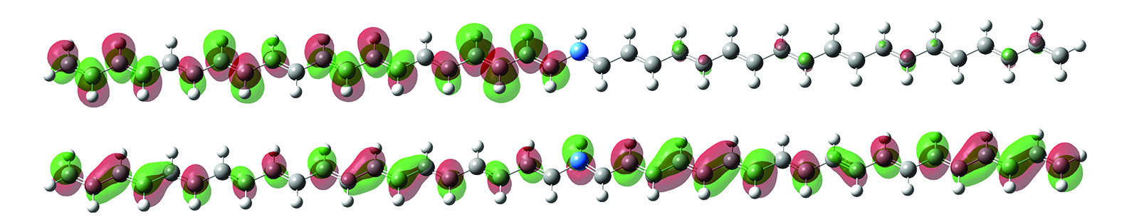
Figure 6. At the bottom of the conductance band, at long Bloch wavelength, the electronic wave function (bottom) in this Gaussian 09 DFT calculation at the 3-21G + level substantially ignores the (blue) Si atom defect, but at shorter Bloch wavelength (top) the backscattering is more severe, localizing the eigenstate to mostly one side.

Figure 7. Numerical results from a simple phonon tight binding simulation of the Raman theory presented in this paper. The calculations involve a 450 unit cell long sample with alternating “bonds” and two or four randomly placed defect impurities. About 3000 placements of the random impurities were averaged here. The $k=0$ and $k=2q$ components can be computed separately (see their contribution to the total in the top row), and their ratio was varied by hand, since we could not do an accurate simulation of the electron localization and backscattering in such a simple model. The lines shapes nonetheless emerge naturally from the simulation and are due to the partial vibrational confinement between ends and defects, seen at the bottom in the simulation and in a Gaussian 09 density functional calculation with four Si atoms in place of carbon. Four low lying vibrational modes are seen, with darkness of the atoms representing vibration amplitude. The vibrational modes have a near linear dispersion in this low $k$ regime and are driven by the constant and sinusoidal terms in the transition moment, as in the tight binding model presented above in figures 2 and 3.

As a check on the mechanisms for lineshape evolution, we constructed a tight binding model with the molecular backbone represented by alternating bonds, of length 450 unit cells, including 2 or 4 randomly placed 10% mass defects. The spectra were calculated for each case by assuming regular, unperturbed constant and sinusoidal driving terms coming from transition moment coordinate dependence of the electronic transitions (we find the electronic states to be much less sensitive to impurities than the vibrations (phonons), which readily semi-localize in zones between impurities, according to our Gaussian 09 DFT calculations). The spectrum was computed by calculating the excitability of each phonon mode of the chain at the given driving “q ’ (with impurities in place), and adding its contribution to the Raman shift spectrum at the mode’s frequency. The sideband backscattering intensity was adjusted by hand and various limits of high and low impurity, long and short molecules, etc. investigated this way. The results for various combinations are shown in figure 7, which should be compared with figures 4,5, and 1. It takes about 3000 random realizations of the impurity positions before the average (shown) settles down.

Implications and conclusion The spectrum of polyacetylene has been explained, in terms of Franck-Condon theory without the Condon approximation. The key is the transition moment and its coordinate dependence, leading to immediate phonon production. In an infinite crystal with delocalized orbitals there is also the absence of new forces in the excited states. Raman sidebands, their dispersion and lineshapes are now understood, requiring backscattering to exist. The theory applied here will be widely applicable to other systems, including graphene. There is a major shift of emphasis from phonons produced after the fact of photoabsorption, to phonons produced instantaneously upon photoabsorption.

For the future, it is important to perform high level electronic structure to map out the transition moment as a function of atomic or phonon displacement. It is important, if difficult perhaps, to experimentally check for the immediate presence of phonons after photoabsorption. This cannot be done by looking for immediate Raman emission in the sidebands, since backscattering must occur first, but the $k=0$ bands should not suffer this, implying an evolution of the sidebands with time in a pulsed experiment.

Acknowledgements The authors acknowledge support from the NSF Center for Integrated Quantum Materials(CIQM) through grant NSF-DMR-1231319. We also thank Prof. Philip Kim for helpful conversations.

References

- [1] Chiang, C. K., et al. Electrical conductivity in doped polyacetylene. Phys. Rev. Lett. 39 1098 (1977).
- [2] Su, W., et.al., Solitons in polyacetylene , Phys. Rev. Let., 42, 1698, (1979).
- [3] Heeger, A.J. et.al., Solitons in conducting polymers Rev. Mod. Phys.60, 781(1988).
- [4] Bryce, M. R., and Munir M. Ahmad Synthetic metals: Polyacetylene and organic superconductors lead the field. Nature 311, : 301-302 (1984).
- [5] Kuzmany, H., Resonance Raman Scattering from Neutral and Doped Polyacetylene, Phys. Stat. Sol. 97, 521-531 (1980).
- [6] Mullazzi, E., et.al., Experimental and theoretical Raman results in trans-polyacetylene Solid State Communications, 46 , 851-855 (1983).
- [7] Ehrenfreund, E., et.al., Amplitude and phase modes in trans-polyacetylene: Resonant Raman scattering and induced infrared activity. Phys. Rev. B, 36 1535 1553, (1987).
- [8] Kuzmany, H.,et.al.,Frank-Condon approach for optical absorption and resonance Raman scattering in trans-polyacetylene. Phys. Rev. B, 26 , 7109 (1982)
- [9] Neto, A. C., et.al., The electronic properties of graphene Rev. Mod. Phys., 81 , 109 (2009); Ferrari, Andrea C. & Basko, Denis M., Raman spectroscopy as a versatile tool for studying the properties of graphene. Nat. Nano. 8, 235–246 (2013).
- [10] Malard, L. M.,et.al., Raman spectroscopy in graphene. Physics Reports 473.5 51-87 (2009).
- [11] see the excellent special issue, Nature Materials, 10, 1-201, (2011).
- [12] C. Castiglioni, et.al., Raman Scattering of Polyconjugated molecules and materials: confinement effect in one and two dimensions, Phil. Trans. R. Soc. London A 362 1448 (2004).
- [13] Jumeau, D., et.al.,Vibrational analysis of trans-polyacetylene : (CH)x and (CD)x. J. Physique 44 819-825 (1983).
- [14] J. G. Duque, et.al., Violation of the Condon Approximation in Semiconducting Carbon Nanotubes. ACS Nano, 5, 5233-5241 (2011).
- [15] Lee, S-Y. & Heller, E.J. . Time-dependent theory of Raman scattering,J. Chem. Phys. 71, 4777-4788 (1979).
- [16] Heller, E.J. et.al., Simple aspects of Raman scattering. J. Phys. Chem. 86, : 1822-1833, (1982).
- [17] Shank, C. V., et al. Picosecond dynamics of photoexcited gap states in polyacetylene, Phys. Rev. Lett. 49, 1660 (1982) .
- [18] Zade, S.S. et.al., From Short Conjugated Oligomers to Conjugated Polymers. Lessons from Studies on Long Conjugated Oligomers. Accts. Chem. Res. 44, 14 24 (2011); see also M. Cardona, in: Light scattering in solids, Vol. 2, eds. M. Cardona and G. Giintherodt 105 (1983)
- [19] Martin, R. M., and Falicov, L. M. , Resonant raman scattering Light scattering in Solids I Springer Berlin Heidelberg, 79-145 (1983).
- [20] Thomsen, C., and Reich S., Double resonant Raman scattering in graphite Phys. Rev. Lett. 85, 5214 (2000) .
- [21] Lee, Soo?Y., Placzek?type polarizability tensors for Raman and resonance Raman scattering, J. Chem. Phys. 78 723-734 (1983).
- [22] Schen, M.A. et.al., Resonant Raman scattering of controlled molecular weight polyacetylene. J. Chem. Phys 89 7615-7620 (1988).
- [23] Schäfer-Siebert, D.,et.al., Influence of the conjugation length of polyacetylene chains on the DC-conductivity. Electronic Properties of Conjugated Polymers Springer Berlin Heidelberg, 38-42 (1987).