Localization and projections on bi–parameter BMO

Abstract.

We prove that for any operator $T$ on bi–parameter BMO the identity factors through $T$ or $\operatorname{Id}-T$. Bourgain’s localization method provides the conceptual framework of our proof. It consists in replacing the factorization problem on the non–separable bi–parameter BMO by its localized, finite dimensional counterpart. We solve the resulting finite dimensional factorization problems by exploiting the geometry and combinatorics of colored dyadic rectangles.

1. Introduction

The dyadic intervals $\mathscr{D}$ on the unit interval are given by

$$\mathscr{D}=\{[2^{-j}k,2^{-j}(k+1)[\,:\,j,k\in\mathbb{N}_{0},k\leq 2^{j}-1\},$$

and the dyadic rectangles $\mathscr{R}$ on the unit square by $\mathscr{R}=\mathscr{D}\times\mathscr{D}$. For any given dyadic interval $I\in\mathscr{D}$ we define the $L^{\infty}$ normalized Haar function $h_{I}$, to be $+1$ on the left half of $I$ and $-1$ on the right half of $I$. Given two dyadic intervals $I,J$ we have

$$h_{I\times J}(s,t)=h_{I}(s)\,h_{J}(t),\qquad s,t\in[0,1[.$$

We define the bi–parameter space $H^{1}(\delta^{2})$ to be the completion of

$$\operatorname{span}\{h_{I\times J}\,:\,I\times J\in\mathscr{R}\}$$

under the norm

$$\|f\|_{H^{1}(\delta^{2})}=\int_{0}^{1}\int_{0}^{1}\big{(}\sum a_{I\times J}^{2}\,h_{I\times J}^{2}\big{)}^{1/2}\,\mathrm{d}s\,\mathrm{d}t,$$ (1.1)

where is the finite linear combination $f=\sum a_{I\times J}h_{I\times J}$. The dual of $H^{1}(\delta^{2})$ is denoted $BMO(\delta^{2})$. It consists of bi–parameter functions $f=\sum a_{I\times J}h_{I\times J}$ with $\|f\|_{BMO(\delta^{2})}<\infty$, where

$$\|f\|_{BMO(\delta^{2})}=\Big{(}\sup_{\Omega\text{ open}}\frac{1}{|\Omega|}\sum_{I\times J\subset\Omega}a_{I\times J}^{2}\,|I\times J|\Big{)}^{1/2}.$$ (1.2)

For basic information and background we refer to [1], [3], [7], [9], [10], [12] and [14].

The main result of this paper is the following theorem.

Theorem 1.1 (Main Theorem).

For any operator

$$S\,:\,BMO(\delta^{2})\rightarrow BMO(\delta^{2})$$

the identity on $BMO(\delta^{2})$ factors through $H=S$ or $H=\operatorname{Id}-S$, that is

$$\vbox{\lx@xy@svg{\hbox{\raise 0.0pt\hbox{\kern 23.90312pt\hbox{\ignorespaces\ignorespaces\ignorespaces\hbox{\vtop{\kern 0.0pt\offinterlineskip\halign{\entry@#!@&&\entry@@#!@\cr&\\&\crcr}}}\ignorespaces{\hbox{\kern-23.90312pt\raise 0.0pt\hbox{\hbox{\kern 0.0pt\raise 0.0pt\hbox{\hbox{\kern 3.0pt\raise 0.0pt\hbox{$\textstyle{BMO(\delta^{2})\ignorespaces\ignorespaces\ignorespaces\ignorespaces\ignorespaces\ignorespaces\ignorespaces\ignorespaces}$}}}}}}}\ignorespaces\ignorespaces\ignorespaces\ignorespaces{}{\hbox{\lx@xy@droprule}}\ignorespaces\ignorespaces\ignorespaces{\hbox{\kern 29.6948pt\raise 5.43056pt\hbox{{}\hbox{\kern 0.0pt\raise 0.0pt\hbox{\hbox{\kern 3.0pt\hbox{\hbox{\kern 0.0pt\raise-2.43056pt\hbox{$\scriptstyle{\operatorname{Id}}$}}}\kern 3.0pt}}}}}}\ignorespaces{\hbox{\kern 47.90312pt\raise 0.0pt\hbox{\hbox{\kern 0.0pt\raise 0.0pt\hbox{\lx@xy@tip{1}\lx@xy@tip{-1}}}}}}{\hbox{\lx@xy@droprule}}{\hbox{\lx@xy@droprule}}\ignorespaces\ignorespaces\ignorespaces\ignorespaces{}{\hbox{\lx@xy@droprule}}\ignorespaces\ignorespaces\ignorespaces{\hbox{\kern-11.57082pt\raise-20.62444pt\hbox{{}\hbox{\kern 0.0pt\raise 0.0pt\hbox{\hbox{\kern 3.0pt\hbox{\hbox{\kern 0.0pt\raise-2.39166pt\hbox{$\scriptstyle{E}$}}}\kern 3.0pt}}}}}}\ignorespaces{\hbox{\kern 0.0pt\raise-29.49998pt\hbox{\hbox{\kern 0.0pt\raise 0.0pt\hbox{\lx@xy@tip{1}\lx@xy@tip{-1}}}}}}{\hbox{\lx@xy@droprule}}{\hbox{\lx@xy@droprule}}{\hbox{\kern 47.90312pt\raise 0.0pt\hbox{\hbox{\kern 0.0pt\raise 0.0pt\hbox{\hbox{\kern 3.0pt\raise 0.0pt\hbox{$\textstyle{BMO(\delta^{2})}$}}}}}}}{\hbox{\kern-23.90312pt\raise-41.24887pt\hbox{\hbox{\kern 0.0pt\raise 0.0pt\hbox{\hbox{\kern 3.0pt\raise 0.0pt\hbox{$\textstyle{BMO(\delta^{2})\ignorespaces\ignorespaces\ignorespaces\ignorespaces}$}}}}}}}\ignorespaces\ignorespaces\ignorespaces\ignorespaces{}{\hbox{\lx@xy@droprule}}\ignorespaces\ignorespaces\ignorespaces{\hbox{\kern 29.70938pt\raise-46.64053pt\hbox{{}\hbox{\kern 0.0pt\raise 0.0pt\hbox{\hbox{\kern 3.0pt\hbox{\hbox{\kern 0.0pt\raise-2.39166pt\hbox{$\scriptstyle{H}$}}}\kern 3.0pt}}}}}}\ignorespaces{\hbox{\kern 47.90312pt\raise-41.24887pt\hbox{\hbox{\kern 0.0pt\raise 0.0pt\hbox{\lx@xy@tip{1}\lx@xy@tip{-1}}}}}}{\hbox{\lx@xy@droprule}}{\hbox{\lx@xy@droprule}}{\hbox{\kern 47.90312pt\raise-41.24887pt\hbox{\hbox{\kern 0.0pt\raise 0.0pt\hbox{\hbox{\kern 3.0pt\raise 0.0pt\hbox{$\textstyle{BMO(\delta^{2})\ignorespaces\ignorespaces\ignorespaces\ignorespaces}$}}}}}}}\ignorespaces\ignorespaces\ignorespaces\ignorespaces{}{\hbox{\lx@xy@droprule}}\ignorespaces\ignorespaces\ignorespaces{\hbox{\kern 71.80624pt\raise-20.62444pt\hbox{{}\hbox{\kern 0.0pt\raise 0.0pt\hbox{\hbox{\kern 3.0pt\hbox{\hbox{\kern 0.0pt\raise-2.39166pt\hbox{$\scriptstyle{P}$}}}\kern 3.0pt}}}}}}\ignorespaces{\hbox{\kern 71.80624pt\raise-5.5pt\hbox{\hbox{\kern 0.0pt\raise 0.0pt\hbox{\lx@xy@tip{1}\lx@xy@tip{-1}}}}}}{\hbox{\lx@xy@droprule}}{\hbox{\lx@xy@droprule}}\ignorespaces}}}}\ignorespaces}\qquad\|E\|\|P\|\leq C, \textstyle{BMO(\delta^{2})\ignorespaces\ignorespaces\ignorespaces\ignorespaces\ignorespaces\ignorespaces\ignorespaces\ignorespaces} \scriptstyle{\operatorname{Id}} \scriptstyle{E} \textstyle{BMO(\delta^{2})} \textstyle{BMO(\delta^{2})\ignorespaces\ignorespaces\ignorespaces\ignorespaces} \scriptstyle{H} \textstyle{BMO(\delta^{2})\ignorespaces\ignorespaces\ignorespaces\ignorespaces} \scriptstyle{P} \textstyle{BMO(\delta^{2})\ignorespaces\ignorespaces\ignorespaces\ignorespaces\ignorespaces\ignorespaces\ignorespaces\ignorespaces} \scriptstyle{\operatorname{Id}} \scriptstyle{E} \textstyle{BMO(\delta^{2})} \textstyle{BMO(\delta^{2})\ignorespaces\ignorespaces\ignorespaces\ignorespaces} \scriptstyle{H} \textstyle{BMO(\delta^{2})\ignorespaces\ignorespaces\ignorespaces\ignorespaces} \scriptstyle{P}$$ (1.3)

where $C>0$ is some universal constant.

As a consequence, $BMO(\delta^{2})$ is a primary Banach space. Recall that a Banach space $X$ is primary if for any projection $S\,:\,X\rightarrow X$ one of the spaces $S(X)$ or $(\operatorname{Id}_{X}-S)(X)$ is isomorphic to $X$. For background on this classical isomorphic invariant concept we refer to [13, 17, 22].

One cannot directly deduce the result that $BMO(\delta^{2})$ is primary from the previously known result that $H^{1}(\delta^{2})$ is primary [16]. To see this, we remark that there exists a projection on $BMO(\delta^{2})$ that is not weak^∗ continuous, and therefore is not the adjoint of an operator on the predual $H^{1}(\delta^{2})$. Indeed, given a Banach limit $\ell:\ell^{\infty}\to\mathbb{R}$ and a collection of disjoint dyadic rectangles $\{R_{1},R_{2},\ldots\}$, let us define the rank one projection $S:BMO(\delta^{2})\to BMO(\delta^{2})$ by

$$Sf=\ell\big{(}(\frac{\langle f,h_{R_{n}}\rangle}{|R_{n}|})_{n=1}^{\infty}\big{)}\sum_{j=1}^{\infty}h_{R_{j}}.$$

One can easily verify that $S$ is a bounded linear projection that is not weak^∗ continuous, since $f_{n}=\sum_{j\geq n}h_{R_{j}}$ is a weak^∗ null sequence and $Sf_{n}=\sum_{j=1}^{\infty}h_{R_{j}}$.

Our proof of the main theorem is based on the localization method introduced by J. Bourgain in [4]. See also [5, 6] and [19] for one of the first papers in this direction. Bourgain’s method is particularly useful for treating factorization problems on non–separable Banach spaces such as $BMO(\delta^{2})$. It aims at replacing (1.3) by its localized, finite dimensional counterpart, and in our context it consists of three basic steps.

1. The starting point consists in applying Wojtaszczyk’s isomorphism [21] to the space $BMO(\delta^{2})$ and its finite dimensional building blocks $BMO_{n}(\delta^{2})=\operatorname{span}\{h_{I\times J}\,:\,I\times J\in\mathscr{R},\,|I|,|J|\geq 2^{-n}\}\operatorname{\cap}BMO(\delta^{2})$. This gives

   $$BMO(\delta^{2})\sim\Big{(}\sum_{n}BMO_{n}(\delta^{2})\Big{)}_{\infty},$$

   where we use the notation $X\sim Y$ to denote that $X$ is isomorphic to $Y$.

2. Reduction to diagonal operators on $\Big{(}\sum_{n}BMO_{n}(\delta^{2})\Big{)}_{\infty}$.

3. Verification of the following finite dimensional and quantitative factorization problem: For any $n\in\mathbb{N}$ and $M>0$ there exists $N=N(n,M)$ such that for any operator $T\,:\,BMO_{N}(\delta^{2})\rightarrow BMO_{N}(\delta^{2})$ with $\|T\|\leq M$ we have that $H=T$ or $H=\operatorname{Id}-T$ satisfies

   $$\vbox{\lx@xy@svg{\hbox{\raise 0.0pt\hbox{\kern 26.45811pt\hbox{\ignorespaces\ignorespaces\ignorespaces\hbox{\vtop{\kern 0.0pt\offinterlineskip\halign{\entry@#!@&&\entry@@#!@\cr&\\&\crcr}}}\ignorespaces{\hbox{\kern-25.58379pt\raise 0.0pt\hbox{\hbox{\kern 0.0pt\raise 0.0pt\hbox{\hbox{\kern 3.0pt\raise 0.0pt\hbox{$\textstyle{BMO_{n}(\delta^{2})\ignorespaces\ignorespaces\ignorespaces\ignorespaces\ignorespaces\ignorespaces\ignorespaces\ignorespaces}$}}}}}}}\ignorespaces\ignorespaces\ignorespaces\ignorespaces{}{\hbox{\lx@xy@droprule}}\ignorespaces\ignorespaces\ignorespaces{\hbox{\kern 32.24979pt\raise 5.43056pt\hbox{{}\hbox{\kern 0.0pt\raise 0.0pt\hbox{\hbox{\kern 3.0pt\hbox{\hbox{\kern 0.0pt\raise-2.43056pt\hbox{$\scriptstyle{\operatorname{Id}}$}}}\kern 3.0pt}}}}}}\ignorespaces{\hbox{\kern 51.33244pt\raise 0.0pt\hbox{\hbox{\kern 0.0pt\raise 0.0pt\hbox{\lx@xy@tip{1}\lx@xy@tip{-1}}}}}}{\hbox{\lx@xy@droprule}}{\hbox{\lx@xy@droprule}}\ignorespaces\ignorespaces\ignorespaces\ignorespaces{}{\hbox{\lx@xy@droprule}}\ignorespaces\ignorespaces\ignorespaces{\hbox{\kern-11.57082pt\raise-20.62444pt\hbox{{}\hbox{\kern 0.0pt\raise 0.0pt\hbox{\hbox{\kern 3.0pt\hbox{\hbox{\kern 0.0pt\raise-2.39166pt\hbox{$\scriptstyle{E}$}}}\kern 3.0pt}}}}}}\ignorespaces{\hbox{\kern 0.0pt\raise-29.49998pt\hbox{\hbox{\kern 0.0pt\raise 0.0pt\hbox{\lx@xy@tip{1}\lx@xy@tip{-1}}}}}}{\hbox{\lx@xy@droprule}}{\hbox{\lx@xy@droprule}}{\hbox{\kern 51.33244pt\raise 0.0pt\hbox{\hbox{\kern 0.0pt\raise 0.0pt\hbox{\hbox{\kern 3.0pt\raise 0.0pt\hbox{$\textstyle{BMO_{n}(\delta^{2})}$}}}}}}}{\hbox{\kern-26.45811pt\raise-41.24887pt\hbox{\hbox{\kern 0.0pt\raise 0.0pt\hbox{\hbox{\kern 3.0pt\raise 0.0pt\hbox{$\textstyle{BMO_{N}(\delta^{2})\ignorespaces\ignorespaces\ignorespaces\ignorespaces}$}}}}}}}\ignorespaces\ignorespaces\ignorespaces\ignorespaces{}{\hbox{\lx@xy@droprule}}\ignorespaces\ignorespaces\ignorespaces{\hbox{\kern 32.26437pt\raise-46.64053pt\hbox{{}\hbox{\kern 0.0pt\raise 0.0pt\hbox{\hbox{\kern 3.0pt\hbox{\hbox{\kern 0.0pt\raise-2.39166pt\hbox{$\scriptstyle{H}$}}}\kern 3.0pt}}}}}}\ignorespaces{\hbox{\kern 50.45811pt\raise-41.24887pt\hbox{\hbox{\kern 0.0pt\raise 0.0pt\hbox{\lx@xy@tip{1}\lx@xy@tip{-1}}}}}}{\hbox{\lx@xy@droprule}}{\hbox{\lx@xy@droprule}}{\hbox{\kern 50.45811pt\raise-41.24887pt\hbox{\hbox{\kern 0.0pt\raise 0.0pt\hbox{\hbox{\kern 3.0pt\raise 0.0pt\hbox{$\textstyle{BMO_{N}(\delta^{2})\ignorespaces\ignorespaces\ignorespaces\ignorespaces}$}}}}}}}\ignorespaces\ignorespaces\ignorespaces\ignorespaces{}{\hbox{\lx@xy@droprule}}\ignorespaces\ignorespaces\ignorespaces{\hbox{\kern 76.91623pt\raise-20.62444pt\hbox{{}\hbox{\kern 0.0pt\raise 0.0pt\hbox{\hbox{\kern 3.0pt\hbox{\hbox{\kern 0.0pt\raise-2.39166pt\hbox{$\scriptstyle{P}$}}}\kern 3.0pt}}}}}}\ignorespaces{\hbox{\kern 76.91623pt\raise-5.5pt\hbox{\hbox{\kern 0.0pt\raise 0.0pt\hbox{\lx@xy@tip{1}\lx@xy@tip{-1}}}}}}{\hbox{\lx@xy@droprule}}{\hbox{\lx@xy@droprule}}\ignorespaces}}}}\ignorespaces}\qquad\|E\|\|P\|\leq C, \textstyle{BMO_{n}(\delta^{2})\ignorespaces\ignorespaces\ignorespaces\ignorespaces\ignorespaces\ignorespaces\ignorespaces\ignorespaces} \scriptstyle{\operatorname{Id}} \scriptstyle{E} \textstyle{BMO_{n}(\delta^{2})} \textstyle{BMO_{N}(\delta^{2})\ignorespaces\ignorespaces\ignorespaces\ignorespaces} \scriptstyle{H} \textstyle{BMO_{N}(\delta^{2})\ignorespaces\ignorespaces\ignorespaces\ignorespaces} \scriptstyle{P} \textstyle{BMO_{n}(\delta^{2})\ignorespaces\ignorespaces\ignorespaces\ignorespaces\ignorespaces\ignorespaces\ignorespaces\ignorespaces} \scriptstyle{\operatorname{Id}} \scriptstyle{E} \textstyle{BMO_{n}(\delta^{2})} \textstyle{BMO_{N}(\delta^{2})\ignorespaces\ignorespaces\ignorespaces\ignorespaces} \scriptstyle{H} \textstyle{BMO_{N}(\delta^{2})\ignorespaces\ignorespaces\ignorespaces\ignorespaces} \scriptstyle{P}$$ (1.4)

   where $C>0$ is some universal constant.

The most challenging aspect in connection with the localization method of Bourgain consists in proving the finite dimensional factorization problem (1.4) while simultaneously controlling $N$ in terms of $n$. The one–parameter factorization problems – solved in [15] – are both the model case and also a special case of our present problem. See also [2, 17, 18, 20].

Organization of the paper

Section 2 lists the preliminary theorems, definitions and concepts. Section 3 states our main technical results (finite dimensional quantitative factorization and almost–diagonalization theorems). Section 4 contains the proof of the almost–diagonalization theorem. Section 5 restates the main theorem (infinite dimensional factorization) and gives its detailed proof.

Acknowledgements

We would like to thank the referee for a careful examination of the manuscript and a very helpful report.

2. Preliminaries

Basic notation

Here we collect basic notation and definitions. We refer to [17] for reference. Recall that $\mathscr{D}$ denotes the dyadic subintervals of the unit interval. Let $\operatorname{\pi}\,:\,\mathscr{D}\setminus\{[0,1)\}\rightarrow\mathscr{D}$ denote the dyadic predecessor map, that is $\operatorname{\pi}(I)=\operatorname*{\bigcap}\{J\in\mathscr{D}\,:\,J\supsetneq I\}$. The level $\operatorname{lev}(I)$ of a dyadic interval $I\in\mathscr{D}$ is defined as $\operatorname{lev}(I)=-\log_{2}(|I|)$. The collection $\mathscr{D}_{j}$ of dyadic intervals at level $j$ is given by $\mathscr{D}_{j}=\{I\in\mathscr{D}\,:\,\operatorname{lev}(I)=j\}$ and we set $\mathscr{D}^{n}=\operatorname*{\bigcup}_{j\leq n}\mathscr{D}_{j}$. For $n\in\mathbb{N}$ we define

$$\mathscr{R}_{n}=\big{\{}I\times J\in\mathscr{R}\,:\,I,J\in\mathscr{D}^{n}\big{\}}.$$

Given a collection of sets $\mathscr{C}$ we define

$$\mathscr{C}^{*}=\operatorname*{\bigcup}\{C\,:\,C\in\mathscr{C}\}.$$

If $A$ is some set, then $\mathscr{C}\operatorname{\cap}A=\{C\operatorname{\cap}A\,:\,C\in\mathscr{C}\}$. The Carleson constant $\llbracket\mathscr{A}\rrbracket$ of a collection $\mathscr{A}\subset\mathscr{D}$ is given by

$$\llbracket\mathscr{A}\rrbracket=\sup_{I\in\mathscr{A}}\sum_{J\in\mathscr{A}\operatorname{\cap}I}|J|/|I|.$$

Note that $\llbracket\mathscr{A}\operatorname{\cup}\mathscr{B}\rrbracket\leq\llbracket\mathscr{A}\rrbracket+\llbracket\mathscr{B}\rrbracket$ for any two collections $\mathscr{A},\mathscr{B}\subset\mathscr{D}$.

For any given dyadic interval $I\in\mathscr{D}$ we define $h_{I}={\mathbbm{1}}_{I_{0}}-{\mathbbm{1}}_{I_{1}}$, where ${\mathbbm{1}}_{A}$ denotes the characteristic function of a set $A$, $I_{0}=[\inf I,(\inf I+\sup I)/2[$ and $I_{1}=[(\inf I+\sup I)/2,\sup I[$. The one parameter hardy space $H^{1}(\delta)$ is the completion of

$$\operatorname{span}\{h_{I}\,:\,I\in\mathscr{D}\}$$

under the square function norm

$$\|f\|_{H^{1}(\delta)}=\int_{0}^{1}\big{(}\sum a_{I}^{2}\,h_{I}^{2}\big{)}^{1/2}\,\mathrm{d}t,$$

where $f=\sum a_{I}h_{I}$. We set

$$H_{n}^{1}(\delta) =\operatorname{span}\{h_{I}\,:\,I\in\mathscr{D}^{n}\}\operatorname{\cap}H^{1}(\delta),$$

$$BMO_{n}(\delta) =\operatorname{span}\{h_{I}\,:\,I\in\mathscr{D}^{n}\}\operatorname{\cap}BMO(\delta).$$

The Gamlen–Gaudet factorization

We recall the relation between large Carleson constants and factorization, see [17]. Let $\mathscr{A}$ be a collection of dyadic intervals satisfying $\llbracket\mathscr{A}\rrbracket\geq N$ and define

$$X_{\mathscr{A}}=\operatorname{span}\{h_{I}\,:\,I\in\mathscr{A}\}\operatorname{\cap}H^{1}(\delta).$$

If $N=n4^{n}$, then there exist linear operators $E$ and $P$ so that

$$\vbox{\lx@xy@svg{\hbox{\raise 0.0pt\hbox{\kern 15.35426pt\hbox{\ignorespaces\ignorespaces\ignorespaces\hbox{\vtop{\kern 0.0pt\offinterlineskip\halign{\entry@#!@&&\entry@@#!@\cr&&\\&&\crcr}}}\ignorespaces{\hbox{\kern-15.35426pt\raise 0.0pt\hbox{\hbox{\kern 0.0pt\raise 0.0pt\hbox{\hbox{\kern 3.0pt\raise 0.0pt\hbox{$\textstyle{H_{n}^{1}(\delta)\ignorespaces\ignorespaces\ignorespaces\ignorespaces\ignorespaces\ignorespaces\ignorespaces\ignorespaces}$}}}}}}}\ignorespaces\ignorespaces\ignorespaces\ignorespaces{}{\hbox{\lx@xy@droprule}}\ignorespaces\ignorespaces\ignorespaces{\hbox{\kern 42.78064pt\raise 5.43056pt\hbox{{}\hbox{\kern 0.0pt\raise 0.0pt\hbox{\hbox{\kern 3.0pt\hbox{\hbox{\kern 0.0pt\raise-2.43056pt\hbox{$\scriptstyle{\operatorname{Id}}$}}}\kern 3.0pt}}}}}}\ignorespaces{\hbox{\kern 82.62367pt\raise 0.0pt\hbox{\hbox{\kern 0.0pt\raise 0.0pt\hbox{\lx@xy@tip{1}\lx@xy@tip{-1}}}}}}{\hbox{\lx@xy@droprule}}{\hbox{\lx@xy@droprule}}\ignorespaces\ignorespaces\ignorespaces{}\ignorespaces\ignorespaces{\hbox{\lx@xy@drawline@}}\ignorespaces\ignorespaces\ignorespaces{\hbox{\kern 13.98584pt\raise-25.36276pt\hbox{{}\hbox{\kern 0.0pt\raise 0.0pt\hbox{\hbox{\kern 3.0pt\hbox{\hbox{\kern 0.0pt\raise-2.39166pt\hbox{$\scriptstyle{E}$}}}\kern 3.0pt}}}}}}\ignorespaces{\hbox{\kern 39.35426pt\raise-32.0952pt\hbox{\hbox{\kern 0.0pt\raise 0.0pt\hbox{\lx@xy@tip{1}\lx@xy@tip{-1}}}}}}\ignorespaces\ignorespaces{\hbox{\lx@xy@drawline@}}\ignorespaces{\hbox{\lx@xy@drawline@}}{\hbox{\kern 45.98897pt\raise 0.0pt\hbox{\hbox{\kern 0.0pt\raise 0.0pt\hbox{\hbox{\kern 3.0pt\raise 0.0pt\hbox{$\textstyle{}$}}}}}}}{\hbox{\kern 82.62367pt\raise 0.0pt\hbox{\hbox{\kern 0.0pt\raise 0.0pt\hbox{\hbox{\kern 3.0pt\raise 0.0pt\hbox{$\textstyle{H_{n}^{1}(\delta)}$}}}}}}}{\hbox{\kern-3.0pt\raise-39.9422pt\hbox{\hbox{\kern 0.0pt\raise 0.0pt\hbox{\hbox{\kern 3.0pt\raise 0.0pt\hbox{$\textstyle{}$}}}}}}}{\hbox{\kern 39.35426pt\raise-39.9422pt\hbox{\hbox{\kern 0.0pt\raise 0.0pt\hbox{\hbox{\kern 3.0pt\raise 0.0pt\hbox{$\textstyle{X_{\mathscr{A}}\ignorespaces\ignorespaces\ignorespaces\ignorespaces}$}}}}}}}\ignorespaces\ignorespaces\ignorespaces{}\ignorespaces\ignorespaces{\hbox{\lx@xy@drawline@}}\ignorespaces\ignorespaces\ignorespaces{\hbox{\kern 72.41968pt\raise-25.36276pt\hbox{{}\hbox{\kern 0.0pt\raise 0.0pt\hbox{\hbox{\kern 3.0pt\hbox{\hbox{\kern 0.0pt\raise-2.39166pt\hbox{$\scriptstyle{P}$}}}\kern 3.0pt}}}}}}\ignorespaces{\hbox{\kern 91.23184pt\raise-5.5pt\hbox{\hbox{\kern 0.0pt\raise 0.0pt\hbox{\lx@xy@tip{1}\lx@xy@tip{-1}}}}}}\ignorespaces\ignorespaces{\hbox{\lx@xy@drawline@}}\ignorespaces{\hbox{\lx@xy@drawline@}}{\hbox{\kern 94.97794pt\raise-39.9422pt\hbox{\hbox{\kern 0.0pt\raise 0.0pt\hbox{\hbox{\kern 3.0pt\raise 0.0pt\hbox{$\textstyle{}$}}}}}}}\ignorespaces}}}}\ignorespaces}\qquad\|E\|\|P\|\leq C. \textstyle{H_{n}^{1}(\delta)\ignorespaces\ignorespaces\ignorespaces\ignorespaces\ignorespaces\ignorespaces\ignorespaces\ignorespaces} \scriptstyle{\operatorname{Id}} \scriptstyle{E} \textstyle{H_{n}^{1}(\delta)} \textstyle{X_{\mathscr{A}}\ignorespaces\ignorespaces\ignorespaces\ignorespaces} \scriptstyle{P} \textstyle{H_{n}^{1}(\delta)\ignorespaces\ignorespaces\ignorespaces\ignorespaces\ignorespaces\ignorespaces\ignorespaces\ignorespaces} \scriptstyle{\operatorname{Id}} \scriptstyle{E} \textstyle{H_{n}^{1}(\delta)} \textstyle{X_{\mathscr{A}}\ignorespaces\ignorespaces\ignorespaces\ignorespaces} \scriptstyle{P}$$ (2.1)

The bi–parameter analogues of these finite dimensional building blocks are:

$$H_{n}^{1}(\delta^{2}) =\operatorname{span}\{h_{I\times J}\,:\,I\times J\in\mathscr{R}_{n}\}\operatorname{\cap}H^{1}(\delta^{2}),$$

$$BMO_{n}(\delta^{2}) =\operatorname{span}\{h_{I\times J}\,:\,I\times J\in\mathscr{R}_{n}\}\operatorname{\cap}BMO(\delta^{2}).$$

In the bi–parameter context, factorization and large Carleson constants are related for collections of rectangles having product structure. Given collections of dyadic intervals $\mathscr{A},\,\mathscr{B}\subset\mathscr{D}$ we define the product space $X_{\mathscr{A}\times\mathscr{B}}$ by

$$X_{\mathscr{A}\times\mathscr{B}}=\operatorname{span}\{h_{I\times J}\,:\,I\times J\in\mathscr{A}\times\mathscr{B}\}\operatorname{\cap}H^{1}(\delta^{2}).$$

If $N=n4^{n}$ and $\llbracket\mathscr{A}\rrbracket\geq N$, $\llbracket\mathscr{B}\rrbracket\geq N$, then there exist linear operators $E$ and $P$ such that

$$\vbox{\lx@xy@svg{\hbox{\raise 0.0pt\hbox{\kern 16.75426pt\hbox{\ignorespaces\ignorespaces\ignorespaces\hbox{\vtop{\kern 0.0pt\offinterlineskip\halign{\entry@#!@&&\entry@@#!@\cr&&\\&&\crcr}}}\ignorespaces{\hbox{\kern-16.75426pt\raise 0.0pt\hbox{\hbox{\kern 0.0pt\raise 0.0pt\hbox{\hbox{\kern 3.0pt\raise 0.0pt\hbox{$\textstyle{H_{n}^{1}(\delta^{2})\ignorespaces\ignorespaces\ignorespaces\ignorespaces\ignorespaces\ignorespaces\ignorespaces\ignorespaces}$}}}}}}}\ignorespaces\ignorespaces\ignorespaces\ignorespaces{}{\hbox{\lx@xy@droprule}}\ignorespaces\ignorespaces\ignorespaces{\hbox{\kern 48.34177pt\raise 5.43056pt\hbox{{}\hbox{\kern 0.0pt\raise 0.0pt\hbox{\hbox{\kern 3.0pt\hbox{\hbox{\kern 0.0pt\raise-2.43056pt\hbox{$\scriptstyle{\operatorname{Id}}$}}}\kern 3.0pt}}}}}}\ignorespaces{\hbox{\kern 92.34593pt\raise 0.0pt\hbox{\hbox{\kern 0.0pt\raise 0.0pt\hbox{\lx@xy@tip{1}\lx@xy@tip{-1}}}}}}{\hbox{\lx@xy@droprule}}{\hbox{\lx@xy@droprule}}\ignorespaces\ignorespaces\ignorespaces{}\ignorespaces\ignorespaces{\hbox{\lx@xy@drawline@}}\ignorespaces\ignorespaces\ignorespaces{\hbox{\kern 17.21838pt\raise-25.5072pt\hbox{{}\hbox{\kern 0.0pt\raise 0.0pt\hbox{\hbox{\kern 3.0pt\hbox{\hbox{\kern 0.0pt\raise-2.39166pt\hbox{$\scriptstyle{E}$}}}\kern 3.0pt}}}}}}\ignorespaces{\hbox{\kern 41.23096pt\raise-30.39777pt\hbox{\hbox{\kern 0.0pt\raise 0.0pt\hbox{\lx@xy@tip{1}\lx@xy@tip{-1}}}}}}\ignorespaces\ignorespaces{\hbox{\lx@xy@drawline@}}\ignorespaces{\hbox{\lx@xy@drawline@}}{\hbox{\kern 51.5501pt\raise 0.0pt\hbox{\hbox{\kern 0.0pt\raise 0.0pt\hbox{\hbox{\kern 3.0pt\raise 0.0pt\hbox{$\textstyle{}$}}}}}}}{\hbox{\kern 92.34593pt\raise 0.0pt\hbox{\hbox{\kern 0.0pt\raise 0.0pt\hbox{\hbox{\kern 3.0pt\raise 0.0pt\hbox{$\textstyle{H_{n}^{1}(\delta^{2})}$}}}}}}}{\hbox{\kern-3.0pt\raise-40.23108pt\hbox{\hbox{\kern 0.0pt\raise 0.0pt\hbox{\hbox{\kern 3.0pt\raise 0.0pt\hbox{$\textstyle{}$}}}}}}}{\hbox{\kern 40.75426pt\raise-40.23108pt\hbox{\hbox{\kern 0.0pt\raise 0.0pt\hbox{\hbox{\kern 3.0pt\raise 0.0pt\hbox{$\textstyle{X_{\mathscr{A}\times\mathscr{B}}\ignorespaces\ignorespaces\ignorespaces\ignorespaces}$}}}}}}}\ignorespaces\ignorespaces\ignorespaces{}\ignorespaces\ignorespaces{\hbox{\lx@xy@drawline@}}\ignorespaces\ignorespaces\ignorespaces{\hbox{\kern 80.31346pt\raise-25.5072pt\hbox{{}\hbox{\kern 0.0pt\raise 0.0pt\hbox{\hbox{\kern 3.0pt\hbox{\hbox{\kern 0.0pt\raise-2.39166pt\hbox{$\scriptstyle{P}$}}}\kern 3.0pt}}}}}}\ignorespaces{\hbox{\kern 101.64511pt\raise-5.5pt\hbox{\hbox{\kern 0.0pt\raise 0.0pt\hbox{\lx@xy@tip{1}\lx@xy@tip{-1}}}}}}\ignorespaces\ignorespaces{\hbox{\lx@xy@drawline@}}\ignorespaces{\hbox{\lx@xy@drawline@}}{\hbox{\kern 106.10019pt\raise-40.23108pt\hbox{\hbox{\kern 0.0pt\raise 0.0pt\hbox{\hbox{\kern 3.0pt\raise 0.0pt\hbox{$\textstyle{}$}}}}}}}\ignorespaces}}}}\ignorespaces}\qquad\|E\|\|P\|\leq C. \textstyle{H_{n}^{1}(\delta^{2})\ignorespaces\ignorespaces\ignorespaces\ignorespaces\ignorespaces\ignorespaces\ignorespaces\ignorespaces} \scriptstyle{\operatorname{Id}} \scriptstyle{E} \textstyle{H_{n}^{1}(\delta^{2})} \textstyle{X_{\mathscr{A}\times\mathscr{B}}\ignorespaces\ignorespaces\ignorespaces\ignorespaces} \scriptstyle{P} \textstyle{H_{n}^{1}(\delta^{2})\ignorespaces\ignorespaces\ignorespaces\ignorespaces\ignorespaces\ignorespaces\ignorespaces\ignorespaces} \scriptstyle{\operatorname{Id}} \scriptstyle{E} \textstyle{H_{n}^{1}(\delta^{2})} \textstyle{X_{\mathscr{A}\times\mathscr{B}}\ignorespaces\ignorespaces\ignorespaces\ignorespaces} \scriptstyle{P}$$ (2.2)

Due to product structure of $X_{\mathscr{A}\times\mathscr{B}}$, the bi–parameter factorization (2.2) results directly from its one–parameter predecessor (2.1). In the next paragraph we discuss Ramsey’s theorem for colored dyadic rectangles. Its relevance for the constructions of this paper comes from the fact that for any two–coloring of $\mathscr{R}_{n}$, Ramsey’s theorem detects a large monochromatic collection of the form $\mathscr{A}\times\mathscr{B}$.

Ramsey theorem for colored dyadic rectangles

Ramsey’s theorem asserts that for any two–coloring of the dyadic rectangles

$$\mathscr{R}_{n}=\big{\{}I\times J\,:\,|I|\geq 2^{-n},\ |J|\geq 2^{-n}\big{\}}$$

there exist collections $\mathscr{A}$, $\mathscr{B}$ of dyadic intervals, each of which has large Carleson constant and, moreover,

$$\mathscr{A}\times\mathscr{B} \mathscr{R}_{n}$$ is monochromatic in .

For later reference we state this assertion in the following theorem.

Theorem 2.1.

Given $n_{0}\in\mathbb{N}$ there exists $n\in\mathbb{N}$ such that for any collection $\mathscr{C}\subset\mathscr{R}_{n}$ one finds $\mathscr{A},\mathscr{B}\subset\mathscr{D}$ satisfying

1. $\mathscr{A}\times\mathscr{B}\subset\mathscr{C}$ or $\mathscr{A}\times\mathscr{B}\subset\mathscr{R}_{n}\setminus\mathscr{C}$,

2. $\llbracket\mathscr{A}\rrbracket\geq n_{0}$ and $\llbracket B\rrbracket\geq n_{0}$.

One can choose $n=n_{0}\,2^{4^{n_{0}}}$.

For the above formulation of Ramsey’s theorem we refer to [16]. See also [11, Chapter 1]. For convenience, we give the proof here.

Proof.

Define $n=n_{0}\,2^{4^{n_{0}}}$ and let $\mathscr{C}\subset\mathscr{R}_{n}$. Define $k=2n_{0}-1$ and let $I_{1},\ldots,I_{2^{k+1}-1}$ be an enumeration of the dyadic intervals in $\mathscr{D}^{k}$. First, we set $\mathscr{E}_{0}=\mathscr{F}_{0}=\mathscr{G}_{0}=\mathscr{D}^{n}$, $I_{0}=\emptyset$ and $f(I_{0})=\infty$. Second, assuming that $\mathscr{E}_{j}$, $\mathscr{F}_{j}$, $\mathscr{G}_{j}$ and $f(I_{j})$ have already been constructed for all $0\leq j\leq m-1$, we define the collections

$$\mathscr{E}_{m}=\{J\in\mathscr{G}_{m-1}\,:\,I_{m}\times J\notin\mathscr{C}\}\quad\text{and}\quad\mathscr{F}_{m}=\{J\in\mathscr{G}_{m-1}\,:\,I_{m}\times J\in\mathscr{C}\}.$$

If $\llbracket\mathscr{E}_{m}\rrbracket\geq\llbracket\mathscr{F}_{m}\rrbracket$, we set $f(I_{m})=0$, and if $\llbracket\mathscr{E}_{m}\rrbracket<\llbracket\mathscr{F}_{m}\rrbracket$, we set $f(I_{m})=1$. To conlude the inductive step, we define $\mathscr{G}_{m}=\mathscr{E}_{m}$ if $f(I_{m})=0$, and $\mathscr{G}_{m}=\mathscr{F}_{m}$ if $f(I_{m})=1$.

Observe that $\mathscr{E}_{m}\cup\mathscr{F}_{m}=\mathscr{G}_{m-1}$ and $\llbracket\mathscr{G}_{m}\rrbracket=\max(\llbracket\mathscr{E}_{m}\rrbracket,\llbracket\mathscr{F}_{m}\rrbracket)$. By subadditivity of $\llbracket\cdot\rrbracket$ we obtain $2\llbracket\mathscr{G}_{m}\rrbracket\geq\llbracket\mathscr{G}_{m-1}\rrbracket$, and by iterating $\llbracket\mathscr{G}_{m}\rrbracket\geq 2^{-m}(n+1)$. For $m=2^{k+1}-1$, we set $\mathscr{B}=\mathscr{G}_{m}$, and observe that by our choices $\llbracket\mathscr{B}\rrbracket\geq 2^{-4^{n_{0}}+1}(n+1)\geq n_{0}$. Now define

$$\mathscr{H}_{0}=\{I\in\mathscr{D}^{k}\,:\,f(I)=0\}\qquad\text{and}\qquad\mathscr{H}_{1}=\{I\in\mathscr{D}^{k}\,:\,f(I)=1\},$$

and note that $\mathscr{H}_{0}\cup\mathscr{H}_{1}=\mathscr{D}^{k}$. By definition of $f$ and $\mathscr{G}_{j}$ we have

$$\mathscr{H}_{0}\times\mathscr{B}\subset(\mathscr{D}^{k}\times\mathscr{D}^{k})\setminus\mathscr{C}\qquad\text{and}\qquad\mathscr{H}_{1}\times\mathscr{B}\subset\mathscr{C}.$$

Now, let $\mathscr{A}=\mathscr{H}_{0}$ if $\llbracket\mathscr{H}_{0}\rrbracket\geq\llbracket\mathscr{H}_{1}\rrbracket$, and $\mathscr{A}=\mathscr{H}_{1}$ if $\llbracket\mathscr{H}_{0}\rrbracket<\llbracket\mathscr{H}_{1}\rrbracket$. We conclude this proof by observing that by our choices we have

$$2\llbracket\mathscr{A}\rrbracket\geq\llbracket\mathscr{H}_{0}\rrbracket+\llbracket\mathscr{H}_{1}\rrbracket\geq\llbracket\mathscr{H}_{0}\cup\mathscr{H}_{1}\rrbracket=\llbracket\mathscr{D}^{k}\rrbracket=k+1=2n_{0}.\qed$$

Block bases and projections in $H^{1}(\delta^{2})$

We introduce next some frequently used terminology and record a boundedness criterion for projections on $H^{1}(\delta^{2})$. We say that a sequence $\{b_{I\times J}\,:\,I\times J\in\mathscr{R}\}$ in a Banach space $X$ is equivalent to the unconditional 2D Haar basis $\{h_{I\times J}\,:\,I\times J\in\mathscr{R}\}$ in $H^{1}(\delta^{2})$ if the following holds: The map

$$T:\sum a_{I\times J}\,h_{I\times J}\to\sum a_{I\times J}\,b_{I\times J}$$

defined initially on finite linear combinations of 2D Haar functions and extended by density to $H^{1}(\delta^{2})$ satisfies

$$C_{1}^{-1}\|x\|_{H^{1}(\delta^{2})}\leq\|T(x)\|_{X}\leq C_{1}\,\|x\|_{H^{1}(\delta^{2})},\quad\quad x\in H^{1}(\delta^{2}).$$

Let $\{\mathscr{E}_{I\times J}:I\times J\in\mathscr{R}\}$ be pairwise disjoint collections of dyadic rectangles and let $E_{I\times J}=\mathscr{E}_{I\times J}^{*}=\operatorname*{\bigcup}\limits_{K\times L\in\mathscr{E}_{I\times J}}K\times L$ be the point-set covered by the collection $\mathscr{E}_{I\times J}$. We denote by

$$b_{I\times J}=\sum_{K\times L\in\mathscr{E}_{I\times J}}h_{K\times L}$$

the block-basis generated by $\mathscr{E}_{I\times J}$. We assume throughout, that $\|b_{I\times J}\|_{2}^{2}=|E_{I\times J}|$ or equivalently that $\mathscr{E}_{I\times J}$ consists of pairwise disjoint dyadic rectangles. We formulate conditions on the collections $\{\mathscr{E}_{I\times J}\}$ so that the block basis $\{b_{I\times J}\}$ is equivalent to the 2D Haar system. The sets $\{E_{I\times J}:I\times J\in\mathscr{R}\}$ satisfy the bi-tree condition if there exists $C_{2}>0$ so that for each $I\times J\in\mathscr{R}$

$$C_{2}^{-1}|I\times J|\leq|E_{I\times J}|\leq C_{2}\,|{I\times J}|.$$ (2.3a)

and for $$(I_{0}\times J_{0}),(I_{1}\times J_{1})\in\mathscr{R} I=\widetilde{I}_{0}=\widetilde{I}_{1} J=\widetilde{J}_{0}=\widetilde{J}_{1}$$ with and we have

$$E_{I_{0}\times J}\operatorname{\cap}E_{I_{1}\times J} =\emptyset, E_{I_{0}\times J}\cup E_{I_{1}\times J} \subset E_{I\times J},$$ (2.3b)

$$E_{I\times J_{0}}\operatorname{\cap}E_{I\times J_{1}} =\emptyset, E_{I\times J_{0}}\cup E_{I\times J_{1}} \subset E_{I\times J}.$$ (2.3c)

If (2.3) is satisfied, then the block basis $\{b_{I\times J}\,:\,I\times J\in\mathscr{R}\}$ is equivalent to the 2D Haar system in$H^{1}(\delta^{2})$ and $C_{1}=C_{1}(C_{2})$. The following theorem is a basic tool that allows to project onto the span of the block bases $\{b_{I\times J}:I\times J\in\mathscr{R}\}$. It was instrumental in proving that $H^{1}(\delta^{2})$ is a primary space, see [8] and [16]. In the present paper, the main component of the factoring operator $P$ appearing in Theorem 1.1 consists of a weighted version of the following orthogonal projection $Q$ onto block basis.

Theorem 2.2.

Let $\mathscr{E}_{I\times J}$, $I\times J\in\mathscr{R}$ be pairwise disjoint collections consisting of disjoint dyadic rectangles. Let $E_{I\times J}=\mathscr{E}_{I\times J}^{*}$. Assume that $\{E_{I\times J}\,:\,I,J\in\mathscr{D}\}$ is a bi-tree, then the following hold

1. The block basis $\{b_{I\times J}:I\times J\in\mathscr{R}\}$ is equivalent to the 2D-Haar basis in $H^{1}(\delta^{2})$ with $C_{1}=C_{1}(C_{2})$.

2. If there exists $C_{3}>0$ so that for each $I\times J,I_{0}\times J_{0}\in\mathscr{R}$ with $I\times J\supset I_{0}\times J_{0}$ and for every $K\times L\in\mathscr{E}_{I\times J}$ we have

   $$C_{3}^{-1}\frac{|E_{I_{0}\times J_{0}}|}{|E_{I\times J}|}\leq\frac{|(K\times L)\operatorname{\cap}E_{I_{0}\times J_{0}}|}{|K\times L|}\leq C_{3}\,\frac{|E_{I_{0}\times J_{0}}|}{|E_{I\times J}|},$$ (2.4)

   then the orthogonal projection

   $$Qf=\sum\langle f,b_{I\times J}\rangle\frac{b_{I\times J}}{\|b_{I\times J}\|_{2}^{2}}$$

   defines a bounded operator on $H^{1}(\delta^{2})$ with norm only depending on $C_{3}$ and $C_{2}$.

Rademacher type functions in $H^{1}(\delta^{2})$ and $BMO(\delta^{2})$

We define the following Rademacher type system as block basis of the Haar system. Given $r\geq k_{0}$ and $K_{0}\times L_{0}\in\mathscr{R}$ with $|K_{0}|=2^{-k_{0}}$ we specify the following functions. First, for any choice of signs we set

$$d_{i}=\sum_{K\in D_{i}\operatorname{\cap}K_{0}}\pm h_{K},\qquad i\geq r.$$

Then it is easy to see that if we define

$$g_{i}(s,t)=d_{i}(s)\,h_{L_{0}}(t),\qquad s,t\in[0,1]$$

for each dyadic interval $L_{0}$, then by (1.1) and duality we have

$$\big{\|}\sum_{i=r}^{r+k-1}g_{i}\big{\|}_{H^{1}(\delta^{2})}=\sqrt{k}|L_{0}|\qquad\text{and}\qquad\big{\|}\sum_{i=r}^{r+k-1}g_{i}\big{\|}_{BMO(\delta)}=\sqrt{k}.$$ (2.5)

3. Localized facorization

Here we prove our quantitative factorization theorem which is one of the three major steps towards the proof of our main theorem.

The main result of this paper is the following quantitative factorization theorem 3.1.

Theorem 3.1.

For $n\in\mathbb{N}$ and $M>0$ there exists $N=N(n,M)$ so that the following holds: For any operator $T\,:\,H_{N}^{1}(\delta^{2})\rightarrow H_{N}^{1}(\delta^{2})$ with $\|T\|\leq M$ the identity on $H_{n}^{1}(\delta^{2})$ factors through $H=T$ or $H=\operatorname{Id}-T$ such that

$$\vbox{\lx@xy@svg{\hbox{\raise 0.0pt\hbox{\kern 17.6286pt\hbox{\ignorespaces\ignorespaces\ignorespaces\hbox{\vtop{\kern 0.0pt\offinterlineskip\halign{\entry@#!@&&\entry@@#!@\cr&\\&\crcr}}}\ignorespaces{\hbox{\kern-16.75426pt\raise 0.0pt\hbox{\hbox{\kern 0.0pt\raise 0.0pt\hbox{\hbox{\kern 3.0pt\raise 0.0pt\hbox{$\textstyle{H_{n}^{1}(\delta^{2})\ignorespaces\ignorespaces\ignorespaces\ignorespaces\ignorespaces\ignorespaces\ignorespaces\ignorespaces}$}}}}}}}\ignorespaces\ignorespaces\ignorespaces\ignorespaces{}{\hbox{\lx@xy@droprule}}\ignorespaces\ignorespaces\ignorespaces{\hbox{\kern 23.42027pt\raise 5.43056pt\hbox{{}\hbox{\kern 0.0pt\raise 0.0pt\hbox{\hbox{\kern 3.0pt\hbox{\hbox{\kern 0.0pt\raise-2.43056pt\hbox{$\scriptstyle{\operatorname{Id}}$}}}\kern 3.0pt}}}}}}\ignorespaces{\hbox{\kern 42.50294pt\raise 0.0pt\hbox{\hbox{\kern 0.0pt\raise 0.0pt\hbox{\lx@xy@tip{1}\lx@xy@tip{-1}}}}}}{\hbox{\lx@xy@droprule}}{\hbox{\lx@xy@droprule}}\ignorespaces\ignorespaces\ignorespaces\ignorespaces{}{\hbox{\lx@xy@droprule}}\ignorespaces\ignorespaces\ignorespaces{\hbox{\kern-11.57082pt\raise-20.62444pt\hbox{{}\hbox{\kern 0.0pt\raise 0.0pt\hbox{\hbox{\kern 3.0pt\hbox{\hbox{\kern 0.0pt\raise-2.39166pt\hbox{$\scriptstyle{E}$}}}\kern 3.0pt}}}}}}\ignorespaces{\hbox{\kern 0.0pt\raise-29.49998pt\hbox{\hbox{\kern 0.0pt\raise 0.0pt\hbox{\lx@xy@tip{1}\lx@xy@tip{-1}}}}}}{\hbox{\lx@xy@droprule}}{\hbox{\lx@xy@droprule}}{\hbox{\kern 42.50294pt\raise 0.0pt\hbox{\hbox{\kern 0.0pt\raise 0.0pt\hbox{\hbox{\kern 3.0pt\raise 0.0pt\hbox{$\textstyle{H_{n}^{1}(\delta^{2})}$}}}}}}}{\hbox{\kern-17.6286pt\raise-41.24887pt\hbox{\hbox{\kern 0.0pt\raise 0.0pt\hbox{\hbox{\kern 3.0pt\raise 0.0pt\hbox{$\textstyle{H_{N}^{1}(\delta^{2})\ignorespaces\ignorespaces\ignorespaces\ignorespaces}$}}}}}}}\ignorespaces\ignorespaces\ignorespaces\ignorespaces{}{\hbox{\lx@xy@droprule}}\ignorespaces\ignorespaces\ignorespaces{\hbox{\kern 23.43486pt\raise-46.64053pt\hbox{{}\hbox{\kern 0.0pt\raise 0.0pt\hbox{\hbox{\kern 3.0pt\hbox{\hbox{\kern 0.0pt\raise-2.39166pt\hbox{$\scriptstyle{H}$}}}\kern 3.0pt}}}}}}\ignorespaces{\hbox{\kern 41.6286pt\raise-41.24887pt\hbox{\hbox{\kern 0.0pt\raise 0.0pt\hbox{\lx@xy@tip{1}\lx@xy@tip{-1}}}}}}{\hbox{\lx@xy@droprule}}{\hbox{\lx@xy@droprule}}{\hbox{\kern 41.6286pt\raise-41.24887pt\hbox{\hbox{\kern 0.0pt\raise 0.0pt\hbox{\hbox{\kern 3.0pt\raise 0.0pt\hbox{$\textstyle{H_{N}^{1}(\delta^{2})\ignorespaces\ignorespaces\ignorespaces\ignorespaces}$}}}}}}}\ignorespaces\ignorespaces\ignorespaces\ignorespaces{}{\hbox{\lx@xy@droprule}}\ignorespaces\ignorespaces\ignorespaces{\hbox{\kern 59.2572pt\raise-20.62444pt\hbox{{}\hbox{\kern 0.0pt\raise 0.0pt\hbox{\hbox{\kern 3.0pt\hbox{\hbox{\kern 0.0pt\raise-2.39166pt\hbox{$\scriptstyle{P}$}}}\kern 3.0pt}}}}}}\ignorespaces{\hbox{\kern 59.2572pt\raise-5.5pt\hbox{\hbox{\kern 0.0pt\raise 0.0pt\hbox{\lx@xy@tip{1}\lx@xy@tip{-1}}}}}}{\hbox{\lx@xy@droprule}}{\hbox{\lx@xy@droprule}}\ignorespaces}}}}\ignorespaces}\qquad\|E\|\|P\|\leq C, \textstyle{H_{n}^{1}(\delta^{2})\ignorespaces\ignorespaces\ignorespaces\ignorespaces\ignorespaces\ignorespaces\ignorespaces\ignorespaces} \scriptstyle{\operatorname{Id}} \scriptstyle{E} \textstyle{H_{n}^{1}(\delta^{2})} \textstyle{H_{N}^{1}(\delta^{2})\ignorespaces\ignorespaces\ignorespaces\ignorespaces} \scriptstyle{H} \textstyle{H_{N}^{1}(\delta^{2})\ignorespaces\ignorespaces\ignorespaces\ignorespaces} \scriptstyle{P} \textstyle{H_{n}^{1}(\delta^{2})\ignorespaces\ignorespaces\ignorespaces\ignorespaces\ignorespaces\ignorespaces\ignorespaces\ignorespaces} \scriptstyle{\operatorname{Id}} \scriptstyle{E} \textstyle{H_{n}^{1}(\delta^{2})} \textstyle{H_{N}^{1}(\delta^{2})\ignorespaces\ignorespaces\ignorespaces\ignorespaces} \scriptstyle{H} \textstyle{H_{N}^{1}(\delta^{2})\ignorespaces\ignorespaces\ignorespaces\ignorespaces} \scriptstyle{P}$$

where $C>0$ is a universal constant.

The proof is based on the following three theorems.

1. Ramsey’s theorem 2.1 for colored dyadic rectangles.

2. The projection theorem 2.2.

3. The almost-diagonalization theorem 3.2 stated below.

These three theorems combined provide the reduction from general operators in theorem 3.1 to multipliers on the Haar system.

The almost-diagonalization theorem

We now state the almost-diagonalization theorem 3.2 and show that in combination with Ramsey’s theorem 2.1 for colored dyadic rectangles and the projection theorem 2.2 it yields the proof of our main result, Theorem 3.1.

Theorem 3.2.

Let $n\in\mathbb{N}$, $M>0$ and $\{\varepsilon_{I\times J}\,:\,I\times J\in\mathscr{R}_{n}\}$ be a given set of small positive scalars. Then there exists $N=N(n,M,\{\varepsilon_{I\times J}\})$ such that for any linear operator $T:H_{N}^{1}(\delta^{2})\rightarrow H_{N}^{1}(\delta^{2})$ with $\|T\|\leq M$ there exist disjoint collections $\mathscr{E}_{I\times J}$, indexed by $I\times J\in\mathscr{R}_{n}$, consisting of pairwise disjoint dyadic rectangles defining the functions

$$b_{I\times J}=\sum_{K\times L\in\mathscr{E}_{I\times J}}h_{K\times L},$$

which satisfy the following conditions:

1. $\mathscr{E}_{I\times J}\subset\mathscr{R}_{N}$ and $|b_{I\times J}|\leq 1$ for all $I\times J\in\mathscr{R}_{n}$.

2. The orthogonal projection

   $$Q(f)=\sum_{I\times J\in\mathscr{R}_{n}}\big{\langle}f,\frac{b_{I\times J}}{\|b_{I\times J}\|_{2}}\big{\rangle}\,\frac{b_{I\times J}}{\|b_{I\times J}\|_{2}}$$

   is a bounded operator on $H^{1}(\delta^{2})$ with $Q(H^{1}(\delta^{2}))=\operatorname{span}\{b_{I\times J}\}$ satisfying

   $$\|Q\,:\,H^{1}(\delta^{2})\to H^{1}(\delta^{2})\|\leq C_{2},$$

   for some universal constant $C_{2}>0$.

3. The map $S\,:\,H_{n}^{1}(\delta^{2})\rightarrow\operatorname{span}\{b_{I\times J}\}\operatorname{\cap}H_{N}^{1}(\delta^{2})$ defined as the linear extension of $h_{I\times J}\mapsto b_{I\times J}$ is an isomorphism with

   $$\|S\|\|S^{-1}\|\leq C_{3},$$ (3.1)

   for some universal constant $C_{3}>0$.

4. We have the estimate

   $$\sum_{K\times L\neq I\times J}|\langle Tb_{K\times L},b_{I\times J}\rangle|\leq\varepsilon_{I\times J}\|b_{I\times J}\|_{2}^{2},$$ (3.2)

   for all $I\times J\in\mathscr{R}_{n}$.

The proof of the almost-diagonalization theorem 3.2 is given in Section 4.

Proof of Theorem 3.1

Let $n\in\mathbb{N}$, $M>0$. We define $N$ by the chain of the following conditions:

$$N =N(N_{1},M,\{\varepsilon_{I\times J}\}), N_{1} =N_{2}\,2^{4^{N_{2}}}, N_{2} =n4^{n},$$ (3.3)

where $\{\varepsilon_{I\times J}\,:\,I\times J\in\mathscr{R}_{N_{1}}\}$ is a collection of positive scalars satisfying

$$\sum_{I\times J\in\mathscr{R}_{N_{1}}}\varepsilon_{I\times J}\leq\frac{1}{4}.$$ (3.4)

Let $T\,:\,H_{N}^{1}(\delta^{2})\rightarrow H_{N}^{1}(\delta^{2})$ be an operator such that $\|T\|\leq M$. Now apply Theorem 3.2 to $T$. This gives a block basis $\{b_{I\times J}\,:\,I\times J\in\mathscr{R}_{N_{1}}\}$ satisfying the conclusions (i)–(3.2) of Theorem 3.2. The Ramsey theorem 2.1 for colored dyadic rectangles applied to

$$\mathscr{C}=\{I\times J\in\mathscr{R}_{N_{1}}\,:\,|\langle Tb_{I\times J},b_{I\times J}\rangle|\geq\|b_{I\times J}\|_{2}^{2}/2\}$$

yields collections $\mathscr{A},\mathscr{B}\subset\mathscr{D}^{N_{1}}$, with Carleson constants $\llbracket\mathscr{A}\rrbracket\geq N_{2}$ and $\llbracket\mathscr{B}\rrbracket\geq N_{2}$, such that $\mathscr{A}\times\mathscr{B}\subset\mathscr{C}$ or $\mathscr{A}\times\mathscr{B}\subset\mathscr{R}_{N_{1}}\setminus\mathscr{C}$. We choose $H=T$ if $\mathscr{A}\times\mathscr{B}\subset\mathscr{C}$ and $H=\operatorname{Id}-T$ if $\mathscr{A}\times\mathscr{B}\subset\mathscr{R}_{N_{1}}\setminus\mathscr{C}$.

The following lower estimate will be essential below:

$$|\langle Hb_{I\times J},b_{I\times J}\rangle|\geq\|b_{I\times J}\|_{2}^{2}/2,\qquad I\times J\in\mathscr{A}\times\mathscr{B}.$$ (3.5)

We define the product space $X_{\mathscr{A}\times\mathscr{B}}$ by

$$X_{\mathscr{A}\times\mathscr{B}}=\operatorname{span}\{h_{I\times J}\,:\,I\times J\in\mathscr{A}\times\mathscr{B}\}\operatorname{\cap}H^{1}(\delta^{2}).$$

Since $\llbracket\mathscr{A}\rrbracket\geq N_{2}$, $\llbracket\mathscr{B}\rrbracket\geq N_{2}$, we know from (2.2) that there exists a universal constant $C>0$ so that

$$\vbox{\lx@xy@svg{\hbox{\raise 0.0pt\hbox{\kern 16.75426pt\hbox{\ignorespaces\ignorespaces\ignorespaces\hbox{\vtop{\kern 0.0pt\offinterlineskip\halign{\entry@#!@&&\entry@@#!@\cr&\\&\crcr}}}\ignorespaces{\hbox{\kern-16.75426pt\raise 0.0pt\hbox{\hbox{\kern 0.0pt\raise 0.0pt\hbox{\hbox{\kern 3.0pt\raise 0.0pt\hbox{$\textstyle{H_{n}^{1}(\delta^{2})\ignorespaces\ignorespaces\ignorespaces\ignorespaces\ignorespaces\ignorespaces\ignorespaces\ignorespaces}$}}}}}}}\ignorespaces\ignorespaces\ignorespaces\ignorespaces{}{\hbox{\lx@xy@droprule}}\ignorespaces\ignorespaces\ignorespaces{\hbox{\kern 22.54593pt\raise 5.43056pt\hbox{{}\hbox{\kern 0.0pt\raise 0.0pt\hbox{\hbox{\kern 3.0pt\hbox{\hbox{\kern 0.0pt\raise-2.43056pt\hbox{$\scriptstyle{\operatorname{Id}}$}}}\kern 3.0pt}}}}}}\ignorespaces{\hbox{\kern 40.75426pt\raise 0.0pt\hbox{\hbox{\kern 0.0pt\raise 0.0pt\hbox{\lx@xy@tip{1}\lx@xy@tip{-1}}}}}}{\hbox{\lx@xy@droprule}}{\hbox{\lx@xy@droprule}}\ignorespaces\ignorespaces\ignorespaces\ignorespaces{}{\hbox{\lx@xy@droprule}}\ignorespaces\ignorespaces\ignorespaces{\hbox{\kern-13.57082pt\raise-20.11554pt\hbox{{}\hbox{\kern 0.0pt\raise 0.0pt\hbox{\hbox{\kern 3.0pt\hbox{\hbox{\kern 0.0pt\raise-1.74722pt\hbox{$\scriptstyle{E_{0}}$}}}\kern 3.0pt}}}}}}\ignorespaces{\hbox{\kern 0.0pt\raise-30.39777pt\hbox{\hbox{\kern 0.0pt\raise 0.0pt\hbox{\lx@xy@tip{1}\lx@xy@tip{-1}}}}}}{\hbox{\lx@xy@droprule}}{\hbox{\lx@xy@droprule}}{\hbox{\kern 40.75426pt\raise 0.0pt\hbox{\hbox{\kern 0.0pt\raise 0.0pt\hbox{\hbox{\kern 3.0pt\raise 0.0pt\hbox{$\textstyle{H_{n}^{1}(\delta^{2})}$}}}}}}}{\hbox{\kern-13.79584pt\raise-40.23108pt\hbox{\hbox{\kern 0.0pt\raise 0.0pt\hbox{\hbox{\kern 3.0pt\raise 0.0pt\hbox{$\textstyle{X_{\mathscr{A}\times\mathscr{B}}\ignorespaces\ignorespaces\ignorespaces\ignorespaces}$}}}}}}}\ignorespaces\ignorespaces\ignorespaces\ignorespaces{}{\hbox{\lx@xy@droprule}}\ignorespaces\ignorespaces\ignorespaces{\hbox{\kern 22.54593pt\raise-34.80052pt\hbox{{}\hbox{\kern 0.0pt\raise 0.0pt\hbox{\hbox{\kern 3.0pt\hbox{\hbox{\kern 0.0pt\raise-2.43056pt\hbox{$\scriptstyle{\operatorname{Id}}$}}}\kern 3.0pt}}}}}}\ignorespaces{\hbox{\kern 43.71268pt\raise-40.23108pt\hbox{\hbox{\kern 0.0pt\raise 0.0pt\hbox{\lx@xy@tip{1}\lx@xy@tip{-1}}}}}}{\hbox{\lx@xy@droprule}}{\hbox{\lx@xy@droprule}}{\hbox{\kern 43.71268pt\raise-40.23108pt\hbox{\hbox{\kern 0.0pt\raise 0.0pt\hbox{\hbox{\kern 3.0pt\raise 0.0pt\hbox{$\textstyle{X_{\mathscr{A}\times\mathscr{B}}\ignorespaces\ignorespaces\ignorespaces\ignorespaces}$}}}}}}}\ignorespaces\ignorespaces\ignorespaces\ignorespaces{}{\hbox{\lx@xy@droprule}}\ignorespaces\ignorespaces\ignorespaces{\hbox{\kern 57.50851pt\raise-20.11554pt\hbox{{}\hbox{\kern 0.0pt\raise 0.0pt\hbox{\hbox{\kern 3.0pt\hbox{\hbox{\kern 0.0pt\raise-1.74722pt\hbox{$\scriptstyle{P_{0}}$}}}\kern 3.0pt}}}}}}\ignorespaces{\hbox{\kern 57.50851pt\raise-5.5pt\hbox{\hbox{\kern 0.0pt\raise 0.0pt\hbox{\lx@xy@tip{1}\lx@xy@tip{-1}}}}}}{\hbox{\lx@xy@droprule}}{\hbox{\lx@xy@droprule}}\ignorespaces}}}}\ignorespaces}\qquad\|E_{0}\|\|P_{0}\|\leq C. \textstyle{H_{n}^{1}(\delta^{2})\ignorespaces\ignorespaces\ignorespaces\ignorespaces\ignorespaces\ignorespaces\ignorespaces\ignorespaces} \scriptstyle{\operatorname{Id}} \scriptstyle{E_{0}} \textstyle{H_{n}^{1}(\delta^{2})} \textstyle{X_{\mathscr{A}\times\mathscr{B}}\ignorespaces\ignorespaces\ignorespaces\ignorespaces} \scriptstyle{\operatorname{Id}} \textstyle{X_{\mathscr{A}\times\mathscr{B}}\ignorespaces\ignorespaces\ignorespaces\ignorespaces} \scriptstyle{P_{0}} \textstyle{H_{n}^{1}(\delta^{2})\ignorespaces\ignorespaces\ignorespaces\ignorespaces\ignorespaces\ignorespaces\ignorespaces\ignorespaces} \scriptstyle{\operatorname{Id}} \scriptstyle{E_{0}} \textstyle{H_{n}^{1}(\delta^{2})} \textstyle{X_{\mathscr{A}\times\mathscr{B}}\ignorespaces\ignorespaces\ignorespaces\ignorespaces} \scriptstyle{\operatorname{Id}} \textstyle{X_{\mathscr{A}\times\mathscr{B}}\ignorespaces\ignorespaces\ignorespaces\ignorespaces} \scriptstyle{P_{0}}$$

We claim that Theorem 3.2 and the choices we made in (3.3),(3.4) and (3.5) imply that there exist linear operators $S_{1}$ and $P_{1}$ such that

$$\vbox{\lx@xy@svg{\hbox{\raise 0.0pt\hbox{\kern 17.6286pt\hbox{\ignorespaces\ignorespaces\ignorespaces\hbox{\vtop{\kern 0.0pt\offinterlineskip\halign{\entry@#!@&&\entry@@#!@\cr&\\&\crcr}}}\ignorespaces{\hbox{\kern-13.79584pt\raise 0.0pt\hbox{\hbox{\kern 0.0pt\raise 0.0pt\hbox{\hbox{\kern 3.0pt\raise 0.0pt\hbox{$\textstyle{X_{\mathscr{A}\times\mathscr{B}}\ignorespaces\ignorespaces\ignorespaces\ignorespaces\ignorespaces\ignorespaces\ignorespaces\ignorespaces}$}}}}}}}\ignorespaces\ignorespaces\ignorespaces\ignorespaces{}{\hbox{\lx@xy@droprule}}\ignorespaces\ignorespaces\ignorespaces{\hbox{\kern 23.42027pt\raise 5.43056pt\hbox{{}\hbox{\kern 0.0pt\raise 0.0pt\hbox{\hbox{\kern 3.0pt\hbox{\hbox{\kern 0.0pt\raise-2.43056pt\hbox{$\scriptstyle{\operatorname{Id}}$}}}\kern 3.0pt}}}}}}\ignorespaces{\hbox{\kern 45.46136pt\raise 0.0pt\hbox{\hbox{\kern 0.0pt\raise 0.0pt\hbox{\lx@xy@tip{1}\lx@xy@tip{-1}}}}}}{\hbox{\lx@xy@droprule}}{\hbox{\lx@xy@droprule}}\ignorespaces\ignorespaces\ignorespaces\ignorespaces{}{\hbox{\lx@xy@droprule}}\ignorespaces\ignorespaces\ignorespaces{\hbox{\kern-12.69582pt\raise-20.11554pt\hbox{{}\hbox{\kern 0.0pt\raise 0.0pt\hbox{\hbox{\kern 3.0pt\hbox{\hbox{\kern 0.0pt\raise-1.74722pt\hbox{$\scriptstyle{S_{1}}$}}}\kern 3.0pt}}}}}}\ignorespaces{\hbox{\kern 0.0pt\raise-28.4822pt\hbox{\hbox{\kern 0.0pt\raise 0.0pt\hbox{\lx@xy@tip{1}\lx@xy@tip{-1}}}}}}{\hbox{\lx@xy@droprule}}{\hbox{\lx@xy@droprule}}{\hbox{\kern 45.46136pt\raise 0.0pt\hbox{\hbox{\kern 0.0pt\raise 0.0pt\hbox{\hbox{\kern 3.0pt\raise 0.0pt\hbox{$\textstyle{X_{\mathscr{A}\times\mathscr{B}}}$}}}}}}}{\hbox{\kern-17.6286pt\raise-40.23108pt\hbox{\hbox{\kern 0.0pt\raise 0.0pt\hbox{\hbox{\kern 3.0pt\raise 0.0pt\hbox{$\textstyle{H_{N}^{1}(\delta^{2})\ignorespaces\ignorespaces\ignorespaces\ignorespaces}$}}}}}}}\ignorespaces\ignorespaces\ignorespaces\ignorespaces{}{\hbox{\lx@xy@droprule}}\ignorespaces\ignorespaces\ignorespaces{\hbox{\kern 23.43486pt\raise-34.83942pt\hbox{{}\hbox{\kern 0.0pt\raise 0.0pt\hbox{\hbox{\kern 3.0pt\hbox{\hbox{\kern 0.0pt\raise-2.39166pt\hbox{$\scriptstyle{H}$}}}\kern 3.0pt}}}}}}\ignorespaces{\hbox{\kern 41.6286pt\raise-40.23108pt\hbox{\hbox{\kern 0.0pt\raise 0.0pt\hbox{\lx@xy@tip{1}\lx@xy@tip{-1}}}}}}{\hbox{\lx@xy@droprule}}{\hbox{\lx@xy@droprule}}{\hbox{\kern 41.6286pt\raise-40.23108pt\hbox{\hbox{\kern 0.0pt\raise 0.0pt\hbox{\hbox{\kern 3.0pt\raise 0.0pt\hbox{$\textstyle{H_{N}^{1}(\delta^{2})\ignorespaces\ignorespaces\ignorespaces\ignorespaces}$}}}}}}}\ignorespaces\ignorespaces\ignorespaces\ignorespaces{}{\hbox{\lx@xy@droprule}}\ignorespaces\ignorespaces\ignorespaces{\hbox{\kern 59.2572pt\raise-20.11554pt\hbox{{}\hbox{\kern 0.0pt\raise 0.0pt\hbox{\hbox{\kern 3.0pt\hbox{\hbox{\kern 0.0pt\raise-1.74722pt\hbox{$\scriptstyle{P_{1}}$}}}\kern 3.0pt}}}}}}\ignorespaces{\hbox{\kern 59.2572pt\raise-5.37999pt\hbox{\hbox{\kern 0.0pt\raise 0.0pt\hbox{\lx@xy@tip{1}\lx@xy@tip{-1}}}}}}{\hbox{\lx@xy@droprule}}{\hbox{\lx@xy@droprule}}\ignorespaces}}}}\ignorespaces}\qquad\|E_{1}\|\|P_{1}\|\leq C, \textstyle{X_{\mathscr{A}\times\mathscr{B}}\ignorespaces\ignorespaces\ignorespaces\ignorespaces\ignorespaces\ignorespaces\ignorespaces\ignorespaces} \scriptstyle{\operatorname{Id}} \scriptstyle{S_{1}} \textstyle{X_{\mathscr{A}\times\mathscr{B}}} \textstyle{H_{N}^{1}(\delta^{2})\ignorespaces\ignorespaces\ignorespaces\ignorespaces} \scriptstyle{H} \textstyle{H_{N}^{1}(\delta^{2})\ignorespaces\ignorespaces\ignorespaces\ignorespaces} \scriptstyle{P_{1}} \textstyle{X_{\mathscr{A}\times\mathscr{B}}\ignorespaces\ignorespaces\ignorespaces\ignorespaces\ignorespaces\ignorespaces\ignorespaces\ignorespaces} \scriptstyle{\operatorname{Id}} \scriptstyle{S_{1}} \textstyle{X_{\mathscr{A}\times\mathscr{B}}} \textstyle{H_{N}^{1}(\delta^{2})\ignorespaces\ignorespaces\ignorespaces\ignorespaces} \scriptstyle{H} \textstyle{H_{N}^{1}(\delta^{2})\ignorespaces\ignorespaces\ignorespaces\ignorespaces} \scriptstyle{P_{1}}$$

for some universal constant $C>0$. For the verification of the claim we remark that the method lined out in [17, 288–290] is directly applicable: The isomorphic embedding

$$S_{1}\,:\,X_{\mathscr{A}\times\mathscr{B}}\to\operatorname{span}\{b_{I\times J}\,:\,I\times J\in\mathscr{A}\times\mathscr{B}\}$$

is defined as the linear extension of the map

$$h_{I\times J}\mapsto b_{I\times J}.$$

For the norm estimate of $S_{1}$ we refer to (3.1). Next, define

$$\widetilde{P}_{1}\,:\,H_{N}^{1}(\delta^{2})\to\operatorname{span}\{b_{I\times J}\,:\,I\times J\in\mathscr{A}\times\mathscr{B}\}$$

by the formula

$$f\mapsto\sum_{I\times J\in\mathscr{A}\times\mathscr{B}}\langle f,b_{I\times J}\rangle b_{I\times J}\langle Hb_{I\times J},b_{I\times J}\rangle^{-1},$$

and observe that $\|\widetilde{P}_{1}\|\leq 2\|Q\|$. We observe that for $g\in\operatorname{span}\{b_{I\times J}\,:\,I\times J\in\mathscr{A}\times\mathscr{B}\}$ we have

$$\widetilde{P}_{1}Hg=g+Gg,$$

where the error term $Gg$ is controlled via $2\sum_{I\times J\in\mathscr{R}_{N_{1}}}\varepsilon_{I\times J}\leq 1/2$ by the following operator norm estimate

$$\big{\|}G\,:\,\operatorname{span}\{b_{I\times J}\,:\,I\times J\in\mathscr{A}\times\mathscr{B}\}\to\operatorname{span}\{b_{I\times J}\,:\,I\times J\in\mathscr{A}\times\mathscr{B}\}\big{\|}_{H^{1}(\delta^{2})}\leq\frac{1}{2}.$$

Hence, we may invert $\operatorname{Id}+G$ on $\operatorname{span}\{b_{I\times J}\,:\,I\times J\in\mathscr{A}\times\mathscr{B}\}$ so that

$$(\operatorname{Id}+G)^{-1}\widetilde{P}_{1}Hg=g,\qquad g\in\operatorname{span}\{b_{I\times J}\,:\,I\times J\in\mathscr{A}\times\mathscr{B}\}.$$

Note that $\|(\operatorname{Id}+G)^{-1}\|\leq 2$. This defines $P_{1}$ as follows:

$$P_{1}f=S_{1}^{-1}(\operatorname{Id}+G)^{-1}\widetilde{P}_{1}f,\qquad f\in X_{\mathscr{A}\times\mathscr{B}}.$$

We should emphasize that $S_{1}^{-1}$ is well defined on the range of $(\operatorname{Id}+G)^{-1}$ and furthermore $(\operatorname{Id}+G)^{-1}$ is well defined on the range of $\widetilde{P}_{1}$.

Finally, it remains to merge the diagrams yielding the following factorization:

$$\vbox{\lx@xy@svg{\hbox{\raise 0.0pt\hbox{\kern 17.6286pt\hbox{\ignorespaces\ignorespaces\ignorespaces\hbox{\vtop{\kern 0.0pt\offinterlineskip\halign{\entry@#!@&&\entry@@#!@\cr&\\&\crcr}}}\ignorespaces{\hbox{\kern-16.75426pt\raise 0.0pt\hbox{\hbox{\kern 0.0pt\raise 0.0pt\hbox{\hbox{\kern 3.0pt\raise 0.0pt\hbox{$\textstyle{H_{n}^{1}(\delta^{2})\ignorespaces\ignorespaces\ignorespaces\ignorespaces\ignorespaces\ignorespaces\ignorespaces\ignorespaces}$}}}}}}}\ignorespaces\ignorespaces\ignorespaces\ignorespaces{}{\hbox{\lx@xy@droprule}}\ignorespaces\ignorespaces\ignorespaces{\hbox{\kern 23.42027pt\raise 5.43056pt\hbox{{}\hbox{\kern 0.0pt\raise 0.0pt\hbox{\hbox{\kern 3.0pt\hbox{\hbox{\kern 0.0pt\raise-2.43056pt\hbox{$\scriptstyle{\operatorname{Id}}$}}}\kern 3.0pt}}}}}}\ignorespaces{\hbox{\kern 42.50294pt\raise 0.0pt\hbox{\hbox{\kern 0.0pt\raise 0.0pt\hbox{\lx@xy@tip{1}\lx@xy@tip{-1}}}}}}{\hbox{\lx@xy@droprule}}{\hbox{\lx@xy@droprule}}\ignorespaces\ignorespaces\ignorespaces\ignorespaces{}{\hbox{\lx@xy@droprule}}\ignorespaces\ignorespaces\ignorespaces{\hbox{\kern-11.57082pt\raise-20.62444pt\hbox{{}\hbox{\kern 0.0pt\raise 0.0pt\hbox{\hbox{\kern 3.0pt\hbox{\hbox{\kern 0.0pt\raise-2.39166pt\hbox{$\scriptstyle{E}$}}}\kern 3.0pt}}}}}}\ignorespaces{\hbox{\kern 0.0pt\raise-29.49998pt\hbox{\hbox{\kern 0.0pt\raise 0.0pt\hbox{\lx@xy@tip{1}\lx@xy@tip{-1}}}}}}{\hbox{\lx@xy@droprule}}{\hbox{\lx@xy@droprule}}{\hbox{\kern 42.50294pt\raise 0.0pt\hbox{\hbox{\kern 0.0pt\raise 0.0pt\hbox{\hbox{\kern 3.0pt\raise 0.0pt\hbox{$\textstyle{H_{n}^{1}(\delta^{2})}$}}}}}}}{\hbox{\kern-17.6286pt\raise-41.24887pt\hbox{\hbox{\kern 0.0pt\raise 0.0pt\hbox{\hbox{\kern 3.0pt\raise 0.0pt\hbox{$\textstyle{H_{N}^{1}(\delta^{2})\ignorespaces\ignorespaces\ignorespaces\ignorespaces}$}}}}}}}\ignorespaces\ignorespaces\ignorespaces\ignorespaces{}{\hbox{\lx@xy@droprule}}\ignorespaces\ignorespaces\ignorespaces{\hbox{\kern 23.43486pt\raise-35.85721pt\hbox{{}\hbox{\kern 0.0pt\raise 0.0pt\hbox{\hbox{\kern 3.0pt\hbox{\hbox{\kern 0.0pt\raise-2.39166pt\hbox{$\scriptstyle{H}$}}}\kern 3.0pt}}}}}}\ignorespaces{\hbox{\kern 41.6286pt\raise-41.24887pt\hbox{\hbox{\kern 0.0pt\raise 0.0pt\hbox{\lx@xy@tip{1}\lx@xy@tip{-1}}}}}}{\hbox{\lx@xy@droprule}}{\hbox{\lx@xy@droprule}}{\hbox{\kern 41.6286pt\raise-41.24887pt\hbox{\hbox{\kern 0.0pt\raise 0.0pt\hbox{\hbox{\kern 3.0pt\raise 0.0pt\hbox{$\textstyle{H_{N}^{1}(\delta^{2})\ignorespaces\ignorespaces\ignorespaces\ignorespaces}$}}}}}}}\ignorespaces\ignorespaces\ignorespaces\ignorespaces{}{\hbox{\lx@xy@droprule}}\ignorespaces\ignorespaces\ignorespaces{\hbox{\kern 59.2572pt\raise-20.62444pt\hbox{{}\hbox{\kern 0.0pt\raise 0.0pt\hbox{\hbox{\kern 3.0pt\hbox{\hbox{\kern 0.0pt\raise-2.39166pt\hbox{$\scriptstyle{P}$}}}\kern 3.0pt}}}}}}\ignorespaces{\hbox{\kern 59.2572pt\raise-5.5pt\hbox{\hbox{\kern 0.0pt\raise 0.0pt\hbox{\lx@xy@tip{1}\lx@xy@tip{-1}}}}}}{\hbox{\lx@xy@droprule}}{\hbox{\lx@xy@droprule}}\ignorespaces}}}}\ignorespaces}\qquad\|E\|\|P\|\leq C, \textstyle{H_{n}^{1}(\delta^{2})\ignorespaces\ignorespaces\ignorespaces\ignorespaces\ignorespaces\ignorespaces\ignorespaces\ignorespaces} \scriptstyle{\operatorname{Id}} \scriptstyle{E} \textstyle{H_{n}^{1}(\delta^{2})} \textstyle{H_{N}^{1}(\delta^{2})\ignorespaces\ignorespaces\ignorespaces\ignorespaces} \scriptstyle{H} \textstyle{H_{N}^{1}(\delta^{2})\ignorespaces\ignorespaces\ignorespaces\ignorespaces} \scriptstyle{P} \textstyle{H_{n}^{1}(\delta^{2})\ignorespaces\ignorespaces\ignorespaces\ignorespaces\ignorespaces\ignorespaces\ignorespaces\ignorespaces} \scriptstyle{\operatorname{Id}} \scriptstyle{E} \textstyle{H_{n}^{1}(\delta^{2})} \textstyle{H_{N}^{1}(\delta^{2})\ignorespaces\ignorespaces\ignorespaces\ignorespaces} \scriptstyle{H} \textstyle{H_{N}^{1}(\delta^{2})\ignorespaces\ignorespaces\ignorespaces\ignorespaces} \scriptstyle{P}$$

where $C>0$ is a universal constant.

4. Quantitative almost-diagonalization

In this section we give the proof of Theorem 3.2. Our argument is inductive. We use induction within the collection of dyadic rectangles. It is therefore important that we introduce a suitable linear ordering relation on the collection of dyadic rectangles. Below we specifically construct the linear ordering relation $\operatorname{\triangleleft\,}$ so that the bijective index function $\cal O_{\operatorname{\triangleleft\,}}\,:\,\mathscr{R}\rightarrow\mathbb{N}$, which is defined by

$$\cal O_{\operatorname{\triangleleft\,}}(R_{0})<\cal O_{\operatorname{\triangleleft\,}}(R_{1})\Leftrightarrow R_{0}\operatorname{\triangleleft\,}R_{1},\qquad R_{0},R_{1}\in\mathscr{R},$$

has the following properties (4.1) and (4.2). For a picture of the index function $\cal O_{\operatorname{\triangleleft\,}}$ see Figure 1. The geometry of a dyadic rectangle and its position within our linear ordering $\operatorname{\triangleleft\,}$ are linked by the inequalities

$$(2^{k}-1)^{2}<\cal O_{\operatorname{\triangleleft\,}}(I\times J)\leq(2^{k+1}-1)^{2},\qquad\text{whenever $\min(|I|,|J|)=2^{-k}$},$$ (4.1)

as well as

$$4\,|I_{1}\times J_{1}|\leq\frac{|I_{0}\times J_{0}|}{\min(|I_{1}|,|J_{1}|)},\qquad\text{whenever $I_{0}\times J_{0}\operatorname{\triangleleft\,}I_{1}\times J_{1}$}.$$ (4.2)

Any linear orderings on the dyadic rectangles for which (4.1) and (4.2) hold may serve as basis for our induction argument in the proof of Theorem 3.2.

4.1. Constructing the linear ordering relation $\operatorname{\triangleleft\,}$ on $\mathscr{R}$

First, we define the rectangles of fixed side lengths $2^{-m}$ and $2^{-n}$ by setting

$$\mathscr{B}_{m,n}=\{I\times J\in\mathscr{R}\,:\,|I|=2^{-m},|J|=2^{-n}\},\qquad m,n\geq 0.$$ (4.3)

Second, we will define the ordering relation $\operatorname{\prec_{\ell}}$ on each of the blocks $\mathscr{B}_{m,n}$. Given two dyadic rectangles $I_{0}\times J_{0},\,I_{1}\times J_{1}\in\mathscr{B}_{m,n}$ we set

$$I_{0}\times J_{0}\operatorname{\prec_{\ell}}I_{1}\times J_{1}\,:\Leftrightarrow(\inf I_{0},\inf J_{0})\operatorname{<_{\ell}}(\inf I_{1},\inf J_{1}),$$

where $\operatorname{<_{\ell}}$ denotes the lexicographic ordering on $\mathbb{R}^{2}$. Third, we shall collect the blocks $\mathscr{B}_{m,n}$ in the collections

$$\mathscr{S}_{k}=\{\mathscr{B}_{m,n}\,:\,\max(m,n)=k\},\qquad k\geq 0.$$

Third, we need to bring the blocks $\mathscr{B}_{m,n}$ in order. To this end, we consider

$$w:\{\mathscr{B}_{m,n}:m,n\geq 0\}\rightarrow\mathbb{N}_{0}$$

such that the following conditions hold for all $k\geq 1$:

1. $w|\mathscr{S}_{k}\,:\,\mathscr{S}_{k}\rightarrow\{k^{2},\ldots,(k+1)^{2}-1\}$ is bijective.

2. we set $w(\mathscr{B}_{0,k})=k^{2}$ and moreover

   $$w(\mathscr{B}_{m_{0},n_{0}})<w(\mathscr{B}_{m_{1},n_{1}})\Leftrightarrow\begin{cases}m_{0}>n_{0}\text{ and }m_{1}\leq n_{1},\\ m_{0}>n_{0}\text{ and }m_{1}>n_{1}\text{ and }n_{0}<n_{1},\\ m_{0}\leq n_{0}\text{ and }m_{1}\leq n_{1}\text{ and }m_{0}<m_{1},\end{cases}$$

   for all $\mathscr{B}_{m_{0},n_{0}},\mathscr{B}_{m_{1},n_{1}}\in\mathscr{S}_{k}\setminus\{\mathscr{B}_{0,k}\}$.

Finally, we use the function $w$ and its properties as well as the properties of $\operatorname{\prec_{\ell}}$ to define our linear ordering relation $\operatorname{\triangleleft\,}$ on the dyadic rectangles $\mathscr{R}$. If $I_{0}\times J_{0},\,I_{1}\times J_{1}\in\mathscr{R}$ we set

$$(I_{0}\times J_{0})\operatorname{\triangleleft\,}(I_{1}\times J_{1}):\Leftrightarrow\begin{cases}w(\mathscr{B}_{\operatorname{lev}I_{0},\operatorname{lev}J_{0}})<w(\mathscr{B}_{\operatorname{lev}I_{1},\operatorname{lev}J_{1}})\text{ or}\\ w(\mathscr{B}_{\operatorname{lev}I_{0},\operatorname{lev}J_{0}})=w(\mathscr{B}_{\operatorname{lev}I_{1},\operatorname{lev}J_{1}})\text{ and }(I_{0},J_{0})\operatorname{\prec_{\ell}}(I_{1},J_{1}).\end{cases}$$

Since our ordering relation $\operatorname{\triangleleft\,}$ is linear, we may well define the bijective index function $\cal O_{\operatorname{\triangleleft\,}}\,:\,\mathscr{R}\rightarrow\mathbb{N}$ by the following property:

$$\cal O_{\operatorname{\triangleleft\,}}(R_{0})<\cal O_{\operatorname{\triangleleft\,}}(R_{1})\Leftrightarrow R_{0}\operatorname{\triangleleft\,}R_{1},\qquad R_{0},R_{1}\in\mathscr{R}.$$

Observe that the crucial relations between the geometry of a dyadic rectangle and its position within our linear ordering (4.1) and (4.2) are satisfied by design.

Figure 1. Index function $\cal O_{\operatorname{\triangleleft\,}}(I\times J)$ for all $I\times J\in\mathscr{R}_{2}$.

4.2. Combinatorial lemma

Let $\{r_{i}\}$ denote the sequence of independent Rademacher functions which are given by

$$r_{i}(t)=\operatorname{sign}(\sin(2\pi 2^{i}t)),\qquad t\in[0,1],\,i\in\mathbb{N}.$$

We consider the tensor product $r_{i,j}$ of the standard Rademacher system defined as

$$r_{ij}(s,t)=r_{i}(s)\,r_{j}(t),\qquad(s,t)\in[0,1]^{2}$$

It is well known and easy to verify that in both spaces, $H^{1}(\delta^{2})$ and $BMO(\delta^{2})$, the system $\{r_{ij}\}$ is equivalent to the unit vector basis of $\ell^{2}$. Specifically, there exists constants $c_{0}$, $C_{0}$ so that for any sequence of scalars $\{a_{ij}\}$ the following inequalities hold.

$$\|\sum a_{ij}r_{ij}\|_{H^{1}(\delta^{2})}^{2}=\sum a_{ij}^{2}$$

and

$$c_{0}\sum a_{ij}^{2}\leq\|\sum a_{ij}r_{ij}\|_{BMO(\delta^{2})}^{2}\leq C_{0}\sum a_{ij}^{2}.$$

Hence, $\{r_{ij}\}$ is a weak null sequence in both spaces $H^{1}(\delta^{2})$ and $BMO(\delta^{2})$,

$$r_{ij}\rightarrow 0\qquad H^{1}(\delta^{2}) i\rightarrow\infty j\rightarrow\infty$$ weakly in , if or

and

$$r_{ij}\rightarrow 0\qquad \text{weakly in $BMO(\delta^{2})$, if $i\rightarrow\infty$ or $j\rightarrow\infty$}.$$

For the purpose of our present work we need a quantitative strengthening of these considerations. This is done in the following combinatorial lemma. Our combinatorial argument is controlled by the local frequency weight

$$f(K\times L)=|\langle x,h_{K\times L}\rangle|+|\langle y,h_{K\times L}\rangle|,\qquad K\times L\subset K_{0}\times L_{0}$$

where $x\in BMO(\delta^{2})$ and $y\in H^{1}(\delta^{2})$ are fixed functions and $K_{0}\times L_{0}\in\mathscr{R}$. For us, it will be extremely important that the collection

$$\{K\times L\,:\,f(K\times L)\leq\tau|K\times L|\}$$

contains almost complete and well–structured coverings of $K_{0}\times L_{0}$ of the form

$$\{K_{0}\times L\,:\,L\in\mathscr{D}_{\ell}\operatorname{\cap}L_{0}\}\qquad\text{and}\qquad\{K\times L_{0}\,:\,K\in\mathscr{D}_{k}\operatorname{\cap}K_{0}\},$$

with $k$ and $\ell$ well under control in terms of $\tau$. See Figure 3.

Lemma 4.1.

Let $i\in\mathbb{N}$, $K_{0},L_{0}\in\mathscr{D}$, $x_{j}\in BMO(\delta^{2})$, $y_{j}\in H^{1}(\delta^{2})$, $1\leq j\leq i$, such that

$$\sum_{j=1}^{i}\|x_{j}\|_{BMO(\delta^{2})}\leq 1\qquad\text{and}\qquad\sum_{j=1}^{i}\|y_{j}\|_{H^{1}(\delta^{2})}\leq|K_{0}\times L_{0}|.$$ (4.4)

Let $\tau>0$, $r\in\mathbb{N}_{0}$, $K\times L\in\mathscr{R}$ and define the local frequency weight

$$f_{i}(K\times L)=\sum_{j=1}^{i}|\langle x_{j},h_{K\times L}\rangle|+|\langle y_{j},h_{K\times L}\rangle|$$ (4.5)

as well as the collections

$$\mathscr{K}(K_{0}\times L_{0}) =\big{\{}K\times L_{0}\,:\,K\subset K_{0},\ |K|\leq 2^{-r}|K_{0}|,\ f_{i}(K\times L_{0})\leq\tau|K\times L_{0}|\big{\}},$$

$$\mathscr{L}(K_{0}\times L_{0}) =\big{\{}K_{0}\times L\,:\,L\subset L_{0},\ |L|\leq 2^{-r}|L_{0}|,\ f_{i}(K_{0}\times L)\leq\tau|K_{0}\times L|\big{\}}.$$

For all integers $k,\ell$ the collections $\mathscr{K}_{k}(K_{0}\times L_{0})$ and $\mathscr{L}_{\ell}(K_{0}\times L_{0})$ are given by

$$\mathscr{K}_{k}(K_{0}\times L_{0}) =\mathscr{K}(K_{0}\times L_{0})\operatorname{\cap}(\{K\in\mathscr{D}\,:\,|K|=2^{-k}|K_{0}|\}\times\mathscr{D}),$$

$$\mathscr{L}_{\ell}(K_{0}\times L_{0}) =\mathscr{L}(K_{0}\times L_{0})\operatorname{\cap}(\mathscr{D}\times\{L\in\mathscr{D}\,:\,|L|=2^{-\ell}|L_{0}|\}).$$

Let $\delta>0$. Then there exist integers $k,\ell$ with

$$r\leq k,\ell\leq\lfloor\frac{i^{2}}{\delta^{2}\tau^{2}}\rfloor+r$$ (4.6)

such that

$$|\mathscr{K}_{k}^{*}(K_{0}\times L_{0})|\geq(1-\delta)|K_{0}\times L_{0}|\quad\text{and}\quad|\mathscr{L}_{\ell}^{*}(K_{0}\times L_{0})|\geq(1-\delta)|K_{0}\times L_{0}|.$$ (4.7)

Proof.

Define $\mathscr{B}=\{K\times L_{0}\,:\,K\subset K_{0}\}\setminus\mathscr{K}(K_{0}\times L_{0})$ and

$$\mathscr{B}_{k}=\mathscr{B}\operatorname{\cap}(\{K\in\mathscr{D}\,:\,|K|=2^{-k}|K_{0}|\}\times\mathscr{D}),$$

see Figure 2.

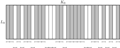
Figure 2. The shaded rectangles form $\mathscr{K}_{k}(K_{0}\times L_{0})$, the white rectangles form $\mathscr{B}_{k}$. The $x$–component of $\mathscr{K}_{k}(K_{0}\times L_{0})$ (first level of intervals) and the $x$–component of $\mathscr{B}_{k}$ (second level of intervals) form a disjoint cover of $K_{0}$.

Let

$$A=\lfloor\frac{i^{2}}{\delta^{2}\tau^{2}}\rfloor+r.$$

By construction $\mathscr{B}_{k}$ and $\mathscr{K}_{k}(K_{0}\times L_{0})$ form a disjoint decomposition of $K_{0}\times L_{0}$. We will determine a collection $\mathscr{K}_{k}(K_{0}\times L_{0})$ by showing that $\mathscr{B}_{k}^{*}$ is small enough for at least one value of $k$. Now assume the opposite, namely that

$$|\mathscr{B}_{k}^{*}|\geq\delta|K_{0}\times L_{0}|,\qquad r\leq k\leq A.$$

Summing these estimates yields

$$\sum_{k=r}^{A}|\mathscr{B}_{k}^{*}|\geq(A-r+1)\,\delta\,|K_{0}\times L_{0}|,$$ (4.8)

Observe that

$$\tau\cdot\sum_{k=r}^{A}|\mathscr{B}_{k}^{*}| \leq\sum_{j=1}^{i}\sum_{k=r}^{A}\sum_{K\times L_{0}\in\mathscr{B}_{k}}|\langle x_{j},h_{K\times L_{0}}\rangle|+|\langle y_{j},h_{K\times L_{0}}\rangle|$$

$$=\sum_{j=1}^{i}\big{|}\big{\langle}x_{j},\sum_{k=r}^{A}\sum_{K\times L_{0}\in\mathscr{B}_{k}}\pm h_{K\times L_{0}}\big{\rangle}\big{|}+\big{|}\big{\langle}y_{j},\sum_{k=r}^{A}\sum_{K\times L_{0}\in\mathscr{B}_{k}}\pm h_{K\times L_{0}}\big{\rangle}\big{|}.$$

By (2.5) we have

$$\Big{\|}\sum_{k=r}^{A}\sum_{K\times L_{0}\in\mathscr{B}_{k}}\pm h_{K\times L_{0}}\Big{\|}_{H^{1}(\delta^{2})} =\sqrt{A-r+1}\ |K_{0}\times L_{0}|,$$

$$\Big{\|}\sum_{k=r}^{A}\sum_{K\times L_{0}\in\mathscr{B}_{k}}\pm h_{K\times L_{0}}\Big{\|}_{BMO(\delta^{2})} =\sqrt{A-r+1},$$

thus, by duality and (4.4) we obtain

$$\tau\cdot\sum_{k=r}^{A}|\mathscr{B}_{k}^{*}|\leq i\,\sqrt{A-r+1}\ |K_{0}\times L_{0}|.$$ (4.9)

Combining (4.8) and (4.9) we conclude

$$A\leq\frac{i^{2}}{\delta^{2}\tau^{2}}+r-1,$$

which contradicts the definition of $A$. Thus we found $r\leq k\leq A$ so that

$$|\mathscr{K}_{k}^{*}(K_{0}\times L_{0})|\geq(1-\delta)|K_{0}\times L_{0}|,$$

see Figure 2. We emphasize that the $x$–component of the rectangles in $\mathscr{K}_{k}^{*}(K_{0}\times L_{0})$ are covering a set of measure $\geq(1-\delta)|K_{0}|$ in $K_{0}$. The $y$–component of the rectangles in $\mathscr{K}_{k}^{*}(K_{0}\times L_{0})$ equals $L_{0}$ throughout. (For the later use of this lemma it is extremely important that we found a large collection of rectangles $\mathscr{K}_{k}(K_{0}\times L_{0})$ where the $y$–component $L_{0}$ remains intact.) See Figure 3.

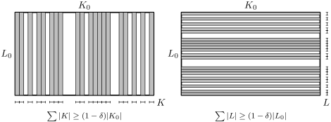
Figure 3. Two good covers. The shaded rectangles in the left picture are from $\mathscr{K}_{k}(K_{0}\times L_{0})$. For those rectangles the $y$–component $L_{0}$ remains intact and the $x$–components $K$ form a large cover of $K_{0}$. Therefore the construction in Section 4.3 yields the crucial measure estimate (4.48). The right picture displays the collection $\mathscr{L}_{\ell}(K_{0}\times L_{0})$ and the roles of $x$ and $y$–components are interchanged.

The same proof in the other variable can be used to show the estimate for $\mathscr{L}_{\ell}^{*}$. ∎

Figure 4. A bad cover of $K_{0}\times L_{0}$. These fragmented shaded rectangles cover the same subset of $K_{0}\times L_{0}$ as $\mathscr{K}_{k}(K_{0}\times L_{0})$ (see Figure 3). The $y$–component $L_{0}$ did not remain intact and therefore the construction in Section 4.3 would not yields the crucial measure estimate (4.48).

4.3. Proof of Theorem 3.2

Theorem 3.2 asserts that we are able to construct a large block basis $\{b_{I\times J}\}$ in $H_{N}^{1}(\delta^{2})$ which are almost eigenvectors for $T$. Moreover, the block basis is such that it spans a well complemented copy of $H_{n}^{1}(\delta^{2})$ in $H_{N}^{1}(\delta^{2})$. We choose the normalization $M=1$ and $\|T\|\leq 1$.

It is here where we will exploit our linear order $\operatorname{\triangleleft\,}$ introduced on the collection of dyadic rectangles $\mathscr{R}$. The proof described below is by mathematical induction executed along the linear order given by $\cal O_{\operatorname{\triangleleft\,}}$.

Inductive construction

To make the transition from standard indexing by dyadic rectangles to indexing by natural numbers we employ the following convention. Given a dyadic rectangle $I\times J$ with $\cal O_{\operatorname{\triangleleft\,}}(I\times J)=i$ we will systematically relabel the collections $\mathscr{E}_{I\times J}$, the functions $b_{I\times J}$ and the constants $\delta_{I\times J}$, $\tau_{I\times J}$ by $\mathscr{E}_{i}$, $b_{i}$ and $\delta_{i}$, $\tau_{i}$, respectively.

Before we begin with our construction we explicitly define the constants $\delta_{i}$ by

$$\delta_{i}=2^{-i}/(8n).$$ (4.10)

The remaining crucial constants $\tau_{i}$ will be defined inductively as the construction proceeds.

First stage of the induction

We begin the induction by setting $\mathscr{E}_{1}:=\mathscr{E}_{[0,1]\times[0,1]}:=\{[0,1]\times[0,1]\}$ and $b_{1}:=b_{[0,1]\times[0,1]}:=h_{[0,1]\times[0,1]}$.

At stage $i$ of the induction

We assume that we have already defined the disjoint collections of dyadic rectangles $\mathscr{E}_{j}$ for all $1\leq j\leq i-1$. Now, we will construct $\mathscr{E}_{i}$. The construction of $\mathscr{E}_{i}$ depends crucially on the value of $i$. We will distinguish between two principal cases, where the second one is divided again into two sub cases.

1. Case 1: The stage ordinal $i$ is given by $i=\cal O_{\operatorname{\triangleleft\,}}([0,1]\times J)$.

2. Case 2: The stage ordinal $i$ is given by $i=\cal O_{\operatorname{\triangleleft\,}}(I\times J)$, where $I\neq[0,1]$.

   1. Case 2.a: The second component $J$ satisfies $J=[0,1]$.

   2. Case 2.b: The second component $J$ satisfies $J\neq[0,1]$.

Case 1: $\bm{I=[0,1]}$. The stage ordinal $i$ is given by $i=\cal O_{\operatorname{\triangleleft\,}}([0,1]\times J)$. Case 1 is applicable to the light rectangles. The collections $\mathscr{E}_{I_{0}\times J_{0}}$ indexed by the dark rectangles $I_{0}\times J_{0}$ are already well defined at this stage. The white ones are ignored.

Recall that

$$b_{j}=\sum_{K\times L\in\mathscr{E}_{j}}h_{K\times L},\qquad 1\leq j\leq i-1.$$

Since the collection $\mathscr{E}_{j}$ consists of pairwise disjoint rectangles we have by (1.1) and duality that

$$\|b_{j}\|_{BMO(\delta^{2})}=1\qquad\text{and}\qquad\|b_{j}\|_{H^{1}(\delta^{2})}=|\mathscr{E}_{j}^{*}|.$$

Let $\widetilde{J}$ denote the unique dyadic interval satisfying $\widetilde{J}\supset J$ and $|\widetilde{J}|=2|J|$. By definition of our linear ordering we have $\cal O_{\operatorname{\triangleleft\,}}([0,1]\times\widetilde{J})\leq i-1$. Hence, $\mathscr{E}_{[0,1]\times\widetilde{J}}$ is already defined. Now put

$$\beta_{i}=\min\{|K_{0}\times L_{0}|\,:\,K_{0}\times L_{0}\in\mathscr{E}_{[0,1]\times\widetilde{J}}\}$$ (4.11)

and define for all $1\leq j\leq i-1$

$$x_{j} :=\frac{1}{i-1}T^{*}b_{j}, y_{j} :=\frac{\beta_{i}}{(i-1)|\mathscr{E}_{j}^{*}|}Tb_{j},$$ (4.12)

Recall that we are using the normalization $\|T\|\leq 1$, hence

$$\sum_{j=1}^{i-1}\|x_{j}\|_{BMO(\delta^{2})}\leq 1\qquad\text{and}\qquad\sum_{j=1}^{i-1}\|y_{j}\|_{H^{1}(\delta^{2})}\leq\beta_{i}.$$

We define the local frequency weight

$$f_{i-1}(K\times L)=\sum_{j=1}^{i-1}|\langle x_{j},h_{K\times L}\rangle|+|\langle y_{j},h_{K\times L}\rangle|,\qquad K\times L\in\mathscr{R}.$$ (4.13)

Given $L_{0}$ we remark that by our previous choices we have the following convenient implication:

$$K\times L_{0}\in\mathscr{E}_{[0,1]\times\widetilde{J}}\quad\text{implies}\quad K=[0,1].$$ (4.14)

We now define the constant $\tau_{i}$ by

$$\tau_{i}=\frac{2^{-i}}{4(i-1)}\beta_{i}\min_{j\leq i}\varepsilon_{j}\|b_{j}\|_{2}^{2}$$ (4.15)

For all $L_{0}$ such that $[0,1]\times L_{0}\in\mathscr{E}_{[0,1]\times\widetilde{J}}$, we define the collection of dyadic rectangles

$$\mathscr{L}([0,1]\times L_{0})=\big{\{}[0,1]\times L\,:\,L\subsetneq L_{0},\ f_{i-1}([0,1]\times L)\leq\tau_{i}|L|\big{\}}.$$

Applying Lemma 4.1 to $\mathscr{L}([0,1]\times L_{0})$ yields an integer $\ell=\ell([0,1]\times L_{0})$ so that

$$1\leq\ell([0,1]\times L_{0})<\frac{(i-1)^{2}}{\delta_{i}^{2}\,\tau_{i}^{2}}+1$$ (4.16)

such that the collection of disjoint dyadic rectangles

$$\mathscr{Z}_{[0,1]\times J}([0,1]\times L_{0})=\big{\{}[0,1]\times L\in\mathscr{L}([0,1]\times L_{0})\,:\,|L|=2^{-\ell([0,1]\times L_{0})}|L_{0}|\big{\}}$$

satisfies the estimate

$$(1-\delta_{i})|[0,1]\times L_{0}|\leq|\mathscr{Z}_{[0,1]\times J}^{*}([0,1]\times L_{0})|\leq|[0,1]\times L_{0}|.$$ (4.17)

Note that in Lemma 4.1 $\mathscr{Z}_{[0,1]\times J}([0,1]\times L_{0})$ was denoted $\mathscr{L}_{\ell}([0,1]\times L_{0})$. Now we take the union and define

$$\mathscr{Z}_{[0,1]\times J}=\operatorname*{\bigcup}\big{\{}\mathscr{Z}_{[0,1]\times J}([0,1]\times L_{0})\,:\,[0,1]\times L_{0}\in\mathscr{E}_{[0,1]\times\widetilde{J}}\big{\}}.$$

Since $\mathscr{Z}_{[0,1]\times J}([0,1]\times L_{0})\subset\mathscr{L}([0,1]\times L_{0})$, we know

$$f_{i-1}([0,1]\times L)\leq\tau_{i}|L|,\qquad\text{for $[0,1]\times L\in\mathscr{Z}_{[0,1]\times J}$}.$$ (4.18)

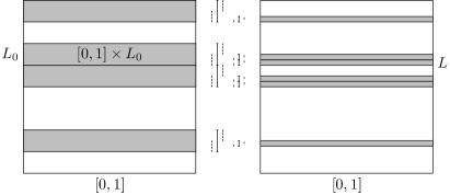
Figure 5. This figure displays the transition from $\mathscr{E}_{[0,1]\times\widetilde{J}}$ to $\mathscr{E}_{[0,1]\times J}$ by means of a generic Gamlen-Gaudet step (4.19). The shaded rectangles $[0,1]\times L_{0}$ on the left form $\mathscr{E}_{[0,1]\times\widetilde{J}}$, the shaded rectangles $[0,1]\times L$ on the right form $\mathscr{E}_{[0,1]\times J}$. The union of the rectangles in $\mathscr{E}_{[0,1]\times J}$ is contained in $E_{[0,1]\times\widetilde{J}}^{\ell}$, since in this figure $J$ is the left half of $\widetilde{J}$. The center displays the $y$–components of $b_{[0,1]\times\widetilde{J}}$ (center left) and of $b_{[0,1]\times J}$ (center right).

We are now ready to define $\mathscr{E}_{[0,1]\times J}$ using the Gamlen-Gaudet procedure. To this end recall first that $\widetilde{J}$ denotes the unique dyadic interval satisfying $\widetilde{J}\supset J$ and $|\widetilde{J}|=2|J|$. For a dyadic interval $L_{0}$ we denote its left half by $L_{0}^{\ell}$ ($L_{0}^{\ell}\subset L_{0}$, $|L_{0}^{\ell}|=|L_{0}|/2$, $\inf L_{0}^{\ell}=\inf L_{0}$) and its right half by $L_{0}^{r}$ ($L_{0}^{r}=L_{0}\setminus L_{0}^{\ell}$). We define the sets

$$E_{[0,1]\times\widetilde{J}}^{\ell}=\operatorname*{\bigcup}_{[0,1]\times L_{0}\in\mathscr{E}_{[0,1]\times\widetilde{J}}}[0,1]\times L_{0}^{\ell}\quad\text{and}\quad E_{[0,1]\times\widetilde{J}}^{r}=\operatorname*{\bigcup}_{[0,1]\times L_{0}\in\mathscr{E}_{[0,1]\times\widetilde{J}}}[0,1]\times L_{0}^{r}.$$

If $J$ is the left half of $\widetilde{J}$, then we put

$$\mathscr{E}_{[0,1]\times J}=\big{\{}[0,1]\times L\in\mathscr{Z}_{[0,1]\times J}\,:\,[0,1]\times L\subset E_{[0,1]\times\widetilde{J}}^{\ell}\big{\}}.$$ (4.19a)

See Figure 5. In the other case when $$J \widetilde{J}$$ is the right half of we put accordingly

$$\mathscr{E}_{[0,1]\times J}=\big{\{}[0,1]\times L\in\mathscr{Z}_{[0,1]\times J}\,:\,[0,1]\times L\subset E_{[0,1]\times\widetilde{J}}^{r}\big{\}}.$$ (4.19b)

Recall that $i=\cal O_{\operatorname{\triangleleft\,}}([0,1]\times J)$ and $\delta_{i}=\delta_{[0,1]\times J}$. An immediate consequence of the Gamlen-Gaudet construction and (4.17) is the estimate

$$\frac{1}{2}(1-\delta_{[0,1]\times J})|[0,1]\times L|\leq|([0,1]\times L)\operatorname{\cap}\mathscr{E}_{[0,1]\times J}^{*}|\leq\frac{1}{2}|[0,1]\times L|,$$ (4.20)

for all $[0,1]\times L\in\mathscr{E}_{[0,1]\times\widetilde{J}}$. Note that all the rectangles in $\mathscr{E}_{[0,1]\times\widetilde{J}}$ are of the form $[0,1]\times L$, see (4.14).

Case 2: $\bm{I\neq[0,1]}$. The figure on the right depicts the transition from Case 1 to Case 2. Here, the stage ordinal $i$ is given by $i=\cal O_{\operatorname{\triangleleft\,}}(I\times J)$ with $I\neq[0,1]$. The rectangle $I\times J$ is one of the light rectangles. The light rectangles fall into two separate cases, see below. Up to (4.33) both cases are treated in tandem.

We will now construct the collections $\mathscr{Y}_{I\times J}$ of $y$–frequencies and depending on each $y$–frequency $L_{0}\in\mathscr{Y}_{I\times J}$ the collection $\mathscr{X}_{I\times J}(L_{0})$ of $x$–frequencies. These frequencies will be our building blocks for $\mathscr{E}_{I\times J}$ and we have

$$\mathscr{E}_{I\times J}\subset\operatorname*{\bigcup}\{\mathscr{X}_{I_{\times}J}(L_{0})\times\{L_{0}\}\,:\,L_{0}\in\mathscr{Y}_{I\times J}\}.$$

The rules by which we finally select $\mathscr{E}_{I\times J}$ from the above large union are given in the equations (4.33).

First, let us define the collection $\mathscr{Y}_{I\times J}$ simply by putting

$$\mathscr{Y}_{I\times J}=\{L_{0}\,:\,[0,1]\times L_{0}\in\mathscr{E}_{[0,1]\times J}\}.$$

We remark that $K\times L_{0}\in\mathscr{E}_{[0,1]\times J}$ implies $K=[0,1]$. Fix $L_{0}\in\mathscr{Y}_{I\times J}$. By means of the combinatorial Lemma 4.1 we will construct the collection $\mathscr{X}_{I\times J}(L_{0})$ of dyadic intervals so that $\mathscr{X}_{I\times J}(L_{0})\times\{L_{0}\}$ is an almost complete cover of $[0,1]\times L_{0}$ and simultaneously the rectangles in $\mathscr{X}_{I\times J}(L_{0})\times\{L_{0}\}$ have almost vanishing local frequency weight (4.13).

Now, let $\mathscr{P}$ denote the previous dyadic rectangle indices that are not located in the same macro block $\mathscr{B}_{m,n}$ as $I\times J$, see (4.3). That is

$$\mathscr{P}=\big{\{}I_{0}\times J_{0}\,:\,I_{0}\times J_{0}\operatorname{\triangleleft\,}I\times J,\,(|I_{0}|,|J_{0}|)\neq(|I|,|J|),\,|I_{0}|\geq|I|,\,|J_{0}|\geq|J|\big{\}},$$

see Figure 6.

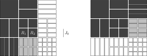
Figure 6. If $I\times J$ is one of the shaded rectangles then $\mathscr{P}$ is the collection of the black rectangles for two generic situations. If $L_{0}^{\prime}$ is defined by (4.21) then $L_{0}^{\prime}\operatorname{\cap}L_{0}\neq\emptyset$ and $L_{0}^{\prime}\subsetneq L_{0}$ is excluded by choice of $\mathscr{P}$. The interval $J_{0}$ defines the strip $\mathscr{D}_{1}\times\{J_{0}\}=\{R_{1},R_{2}\}$ in $\mathbb{A}$, see (4.22).

For each $I_{0}\times J_{0}\in\mathscr{P}$ there exists a unique $L_{0}^{\prime}\in\mathscr{Y}_{I_{0}\times J_{0}}$ such that $L_{0}^{\prime}\operatorname{\cap}L_{0}\neq\emptyset$ in which case $L_{0}^{\prime}\supset L_{0}$, see Figure 6. We display the logical dependence by writing

$$L_{0}^{\prime}=L_{0}^{\prime}(I\times J,L_{0},I_{0}\times J_{0}).$$ (4.21)

Next, we further partition $\mathscr{P}$ into strip collections. Recall that $\mathscr{D}_{m}=\{I\in\mathscr{D}\,:\,|I|=2^{-m}\}$. We define $\mathbb{A}$ by the following rule: if $I_{0}\times J_{0}\in\mathscr{P}$ and $|I_{0}|=2^{-m}$ we put $\mathscr{D}_{m}\times\{J_{0}\}\in\mathbb{A}$. In other words

$$\mathbb{A}=\big{\{}\mathscr{D}_{m}\times\{J_{0}\}\,:\,m\in\mathbb{N}_{0},\,I_{0}\times J_{0}\in\mathscr{P},\,I_{0}\in\mathscr{D}_{m}\big{\}}.$$ (4.22)

See Figure 6. Note that if $\mathscr{S}\in\mathbb{A}$ then there exist $m$ and $J_{0}\in\mathscr{D}$ such that $\mathscr{S}=\mathscr{D}_{m}\times\{J_{0}\}$ and for each $I_{0}^{\prime}\in\mathscr{D}_{m}$ we have $I_{0}^{\prime}\times J_{0}\in\mathscr{P}$. We have clearly $\mathscr{P}=\operatorname*{\bigcup}_{\mathscr{S}\in\mathbb{A}}\mathscr{S}$.

After the preperatory step above we now turn to the core construction, which uses $\mathscr{X}_{I_{0}\times J_{0}}(L_{0}^{\prime})$, $I_{0}\times J_{0}\in\mathscr{P}$ as input and returns the collection $\mathscr{X}_{I\times J}(L_{0})$ as output. We extract the relevant information carried by the input collection by defining the following sets:

$$W_{I\times J}(\mathscr{S},L_{0})=\operatorname*{\bigcup}\big{\{}\mathscr{X}_{I_{0}\times J_{0}}^{*}(L_{0}^{\prime})\,:\,I_{0}\times J_{0}\in\mathscr{S}\big{\}},\qquad\mathscr{S}\in\mathbb{A}.$$ (4.23)

(We emphasize the logical dependece $L_{0}^{\prime}=L_{0}^{\prime}(I\times J,L_{0},I_{0}\times J_{0})$.) See Figure 7.

Figure 7. From top to bottom the figure describes the transition from the input data $W_{I\times J}(\mathscr{S},L_{0})$ to their intersection $W_{I\times J}(L_{0})$ to the fine covering $\mathscr{W}_{I\times J}(L_{0})$ and the rectangles $\mathscr{W}_{I\times J}(L_{0})\times\{L_{0}\}$. The refinement $\mathscr{X}_{I\times J}(L_{0})\times\{L_{0}\}$ of $\mathscr{W}_{I\times J}(L_{0})\times\{L_{0}\}$ results from Lemma 4.1, hence $(K_{0}\operatorname{\cap}\mathscr{X}_{I\times J}(L_{0}))\times\{L_{0}\}$ almost covers $K_{0}\times L_{0}$.

Now we take the intersection over the strips $\mathscr{S}\in\mathbb{A}$

$$W_{I\times J}(L_{0})=\operatorname*{\bigcap}_{\mathscr{S}\in\mathbb{A}}W_{I\times J}(\mathscr{S},L_{0}).$$

We next choose a fine covering of $W_{I\times J}(L_{0})$ by intervals of equal length. To this we put

$$\eta_{i}=\frac{1}{2}\min\{|K|\,:\,\exists L,\,K\times L\in\operatorname*{\bigcup}_{I_{0}\times J_{0}\in\mathscr{P}}\mathscr{E}_{I_{0}\times J_{0}}\},$$

and set

$$\mathscr{W}_{I\times J}(L_{0})=\{K\in\mathscr{D}\,:\,|K|=\eta_{i},\,K\subset W_{I\times J}(L_{0})\}.$$

The collection of intervals $\mathscr{W}_{I\times J}(L_{0})$ gives rise to the collection of pairwise disjoint dyadic rectangles $\mathscr{W}_{I\times J}(L_{0})\times\{L_{0}\}$, see Figure 7. By means of the combinatorial Lemma 4.1 we refine this collection of rectangles and obtain a almost complete covering of $W_{I\times J}(L_{0})\times\{L_{0}\}$ consisting of rectangles $K\times L_{0}$ with almost vanishing local frequency weight $f_{i-1}$ specified below. It is important that in the refined covering the $y$–component $L_{0}$ remains intact.

We defined previously that

$$b_{j}=\sum_{K\times L\in\mathscr{E}_{j}}h_{K\times L},\qquad 1\leq j\leq i-1.$$

Since the collection $\mathscr{E}_{j}$ consists of pairwise disjoint rectangles we have by (1.1) and duality that

$$\|b_{j}\|_{BMO(\delta^{2})}=1\qquad\text{and}\qquad\|b_{j}\|_{H^{1}(\delta^{2})}=|\mathscr{E}_{j}^{*}|.$$

Now, put

$$\beta_{i}=\min\{|K_{0}\times L_{0}|\,:\,L_{0}\in\mathscr{Y}_{I\times J},K_{0}\in\mathscr{W}_{I\times J}(L_{0})\}$$ (4.24)

and define for all $1\leq j\leq i-1$

$$x_{j} :=\frac{1}{i-1}T^{*}b_{j}, y_{j} :=\frac{\beta_{i}}{(i-1)|\mathscr{E}_{j}^{*}|}Tb_{j},$$ (4.25)

Recall that we are using the normalization $\|T\|\leq 1$, hence

$$\sum_{j=1}^{i-1}\|x_{j}\|_{BMO(\delta^{2})}\leq 1\qquad\text{and}\qquad\sum_{j=1}^{i-1}\|y_{j}\|_{H^{1}(\delta^{2})}\leq\beta_{i}.$$

We next define the local frequency weight

$$f_{i-1}(K\times L)=\sum_{j=1}^{i-1}|\langle x_{j},h_{K\times L}\rangle|+|\langle y_{j},h_{K\times L}\rangle|,\qquad K\times L\in\mathscr{R}.$$ (4.26)

We fix $K_{0}\in\mathscr{W}_{I\times J}(L_{0})$ and let

$$\mathscr{K}(K_{0}\times L_{0})=\{K\times L_{0}\,:\,K\subsetneq K_{0},\,f_{i-1}(K\times L_{0})\leq\tau_{i}|K\times L_{0}|\},$$

where the constant $\tau_{i}$ is given by

$$\tau_{i}=\frac{2^{-i}}{4(i-1)}\beta_{i}\min_{j\leq i}\varepsilon_{j}\|b_{j}\|_{2}^{2}.$$ (4.27)

Applying Lemma 4.1 to $\mathscr{K}(K_{0}\times L_{0})$ yields an integer $k=k(K_{0}\times L_{0})$ such that

$$1\leq k(K_{0}\times L_{0})<\frac{(i-1)^{2}}{\delta_{i}^{2}\,\tau_{i}^{2}}+1$$ (4.28)

and so that

$$\mathscr{Z}_{I\times J}(K_{0}\times L_{0})=\big{\{}K\times L_{0}\in\mathscr{K}(K_{0}\times L_{0})\,:\,|K|=2^{-k(K_{0}\times L_{0})}|K_{0}|\big{\}}$$

satisfies

$$(1-\delta_{i})|K_{0}\times L_{0}|\leq|\mathscr{Z}_{I\times J}^{*}(K_{0}\times L_{0})|\leq|K_{0}\times L_{0}|.$$ (4.29)

Finally, the result of our construction is thus

$$\mathscr{X}_{I\times J}(L_{0})=\{K\,:\,K\times L_{0}\in\mathscr{Z}_{I\times J}(K_{0}\times L_{0}),K_{0}\in\mathscr{W}_{I\times J}(L_{0})\},$$ (4.30)

and

$$\mathscr{Z}_{I\times J}=\operatorname*{\bigcup}\big{\{}\mathscr{X}_{I\times J}(L_{0})\times\{L_{0}\}\,:\,L_{0}\in\mathscr{Y}_{I\times J}\big{\}}.$$ (4.31)

Observe that the following identity holds:

$$\mathscr{Z}_{I\times J}=\operatorname*{\bigcup}\big{\{}\mathscr{Z}_{I\times J}(K_{0}\times L_{0})\,:\,L_{0}\in\mathscr{Y}_{I\times J},\,K_{0}\in\mathscr{W}_{I\times J}(L_{0})\big{\}}.$$

Since $\mathscr{Z}_{I\times J}(K_{0}\times L_{0})\subset\mathscr{K}(K_{0}\times L_{0})$, we have the estimate

$$f_{i-1}(K\times L_{0})\leq\tau_{i}|K\times L_{0}|,\qquad\text{for all $K\times L_{0}\in\mathscr{Z}_{I\times J}$.}$$ (4.32)

Up to this point, the construction for Case 2.a and Case 2.b are identical. Now is the time to distinguish between the cases $J=[0,1]$ and $J\neq[0,1]$.

Case 2.a: $$\bm{I\neq[0,1]} \bm{J=[0,1]} I\times J \mathscr{E}_{I\times J} \mathscr{E}_{I_{0}\times J_{0}} I_{0}\times J_{0}$$, . The light rectangles are the ones to which Case 2.a is applicable. The collection is defined in (4.33a). The collections indexed by the dark rectangles are already well defined. The white ones are ignored.

We are now ready to define $\mathscr{E}_{I\times J}$ using the Gamlen-Gaudet procedure. To this end recall first that $\widetilde{I}$ denotes the unique dyadic interval satisfying $\widetilde{I}\supset I$ and $|\widetilde{I}|=2|I|$. Second, for a dyadic interval $K_{0}$ we denote its left half by $K_{0}^{\ell}$ ($K_{0}^{\ell}\subset K_{0}$, $|K_{0}^{\ell}|=|K_{0}|/2$, $\inf K_{0}^{\ell}=\inf K_{0}$) and its right half by $K_{0}^{r}$ ($K_{0}^{r}=K_{0}\setminus K_{0}^{\ell}$). We define the sets

$$E_{\widetilde{I}\times J}^{\ell}=\operatorname*{\bigcup}_{K_{0}\times L_{0}\in\mathscr{E}_{\widetilde{I}\times J}}K_{0}^{\ell}\times L_{0}\quad\text{and}\quad E_{\widetilde{I}\times J}^{r}=\operatorname*{\bigcup}_{K_{0}\times L_{0}\in\mathscr{E}_{\widetilde{I}\times J}}K_{0}^{r}\times L_{0}.$$

If $I$ is the left half of $\widetilde{I}$, then we put

$$\mathscr{E}_{I\times J}=\{K\times L_{0}\in\mathscr{Z}_{I\times J}\,:\,K\times L_{0}\subset E_{\widetilde{I}\times J}^{\ell}\},$$ (4.33a)

Alternatively, if $I$ is the right half of $\widetilde{I}$, then

$$\mathscr{E}_{I\times J}=\{K\times L_{0}\in\mathscr{Z}_{I\times J}\,:\,K\times L_{0}\subset E_{\widetilde{I}\times J}^{r}\}.$$ (4.33b)

Case 2.b: $\bm{I\neq[0,1]}$, $\bm{J\neq[0,1]}$. The figure on the right depicts the transition from Case 2.a to Case 2.b. The light rectangles $I\times J$ are the ones covered by Case 2.b. The collection $\mathscr{E}_{I\times J}$ is defined in (4.33c). The collections $\mathscr{E}_{I_{0}\times J_{0}}$ indexed by the dark rectangles $I_{0}\times J_{0}$ are well defined before the first light rectangle is treated.

$$\mathscr{E}_{I\times J}=\{K\times L_{0}\in\mathscr{Z}_{I\times J}\,:\,K\times L_{0}\subset\mathscr{E}_{I\times\widetilde{J}}^{*}\}$$ (4.33c)

(A comment on (4.33c): It is here where we bring in the combinatorial harvest of Lemma 4.1 where we insisted that the coverings leave the $y$–components $L_{0}$ intact, see Figure 3. Moreover, the definition (4.33c) would not be possible if we used fragmented coverings as depicted in Figure 4.)

In each of the above cases (4.33) we put

$$b_{I\times J}=\sum_{K\times L\in\mathscr{E}_{I\times J}}h_{K\times L}.$$ (4.34)

A first property of $\mathscr{E}_{I\times J}$

We have now completed the construction part of the proof. Before we turn to a detailed examination of the entire system $\{\mathscr{E}_{I\times J}\,:\,I\times J\in\mathscr{R}\}$ and $\{b_{I\times J}\,:\,I\times J\in\mathscr{R}\}$ we analyze the intersections $K\times L\operatorname{\cap}\mathscr{E}_{I\times J}^{*}$ where $K\times L\in\mathscr{E}_{\widetilde{I}\times J}\operatorname{\cup}\mathscr{E}_{I\times\widetilde{J}}$. Put

$$1-\alpha_{I\times J}=\prod_{I_{0}\times J_{0}\operatorname{\trianglelefteq\,}I\times J}(1-\delta_{I_{0}\times J_{0}})^{2}.$$

We claim that

$$\frac{1}{2}(1-\alpha_{I\times J})|K\times L|\leq|(K\times L)\operatorname{\cap}\mathscr{E}_{I\times J}^{*}|\leq\frac{1}{2}|K\times L|,$$ (4.35a)

for all $$K\times L\in\mathscr{E}_{\widetilde{I}\times J} I\neq[0,1]$$ if , as well as

$$\frac{1}{2}(1-\alpha_{I\times J})|K\times L|\leq|(K\times L)\operatorname{\cap}\mathscr{E}_{I\times J}^{*}|\leq\frac{1}{2}|K\times L|,$$ (4.35b)

for all $$K\times L\in\mathscr{E}_{I\times\widetilde{J}} J\neq[0,1]$$ if .

Indeed, we only have to verify the left hand side estimates. First, let $K\times L\in\mathscr{E}_{\widetilde{I}\times J}$. Observe that since $\mathscr{Y}_{\widetilde{I}\times J}=\mathscr{Y}_{I\times J}$ and $|\mathscr{E}_{I\times J}^{*}\operatorname{\cap}([0,1]\times L)|=\frac{1}{2}|\mathscr{X}_{I\times J}^{*}(L)\times L|$ for all $L\in\mathscr{Y}_{I\times J}$, we have

$$|(K\times L)\operatorname{\cap}\mathscr{E}_{I\times J}^{*}|=\frac{1}{2}|(K\times L)\operatorname{\cap}(\mathscr{X}_{I\times J}^{*}(L)\times L)|.$$ (4.36)

Obviously, by (4.29), the right hand side is larger than

$$\frac{1}{2}(1-\delta_{I\times J})|K\operatorname{\cap}W_{I\times J}(L)|\,|L|.$$ (4.37)

We go back over the course by which we have come and see that

$$|K\operatorname{\cap}W_{I\times J}(L)|\geq\prod_{\widetilde{I}\times J\operatorname{\triangleleft\,}I_{0}\times J_{0}\operatorname{\triangleleft\,}I\times J}(1-\delta_{I_{0}\times J_{0}})|K|.$$ (4.38)

Combining (4.36), with (4.37) and (4.38) yields (4.35a). Second, let $K\times L\in\mathscr{E}_{I\times\widetilde{J}}$ and $J\neq[0,1]$. By the definition of $\mathscr{E}_{I\times J}$ and (4.31) we have

$$|(K\times L)\operatorname{\cap}\mathscr{E}_{I\times J}^{*}|=\sum_{L_{0}\in\mathscr{Y}_{I\times J}}|(K\times L)\operatorname{\cap}(\mathscr{X}_{I\times J}^{*}(L_{0})\times L_{0})|.$$ (4.39)

For each summand note the identity

$$|(K\times L)\operatorname{\cap}(\mathscr{X}_{I\times J}^{*}(L_{0})\times L_{0})|=|K\operatorname{\cap}\mathscr{X}_{I\times J}^{*}(L_{0})|\,|L\operatorname{\cap}L_{0}|.$$ (4.40)

As before, we have

$$|K\operatorname{\cap}\mathscr{X}_{I\times J}^{*}(L_{0})|\geq(1-\delta_{I\times J})|K\operatorname{\cap}W_{I\times J}(L_{0})|$$ (4.41)

and

$$|K\operatorname{\cap}W_{I\times J}(L_{0})|\geq\prod_{I\times\widetilde{J}\operatorname{\triangleleft\,}I_{0}\times J_{0}\operatorname{\triangleleft\,}I\times J}(1-\delta_{I_{0}\times J_{0}})|K|.$$ (4.42)

Next, we observe that by (4.40), (4.41) and (4.42), the sum in the right hand side of (4.39) is larger than

$$\Big{(}\prod_{I\times\widetilde{J}\operatorname{\triangleleft\,}I_{0}\times J_{0}\operatorname{\trianglelefteq\,}I\times J}(1-\delta_{I_{0}\times J_{0}})\Big{)}|K|\sum_{L_{0}\in\mathscr{Y}_{I\times J}}|L\operatorname{\cap}L_{0}|.$$ (4.43)

Taking into account that $J\subset\widetilde{J}$, the Gamlen-Gaudet construction of Case 1 gives

$$\sum_{L_{0}\in\mathscr{Y}_{I\times J}}|L\operatorname{\cap}L_{0}|\geq\frac{1}{2}(1-\delta_{[0,1]\times J})|L|.$$ (4.44)

Finally, combining (4.43) and (4.44) with (4.39) yields (4.35b).

Essential properties of our construction

Output of the inductive step

Having completed the construction of $\{\mathscr{E}_{I\times J}\,:\,I\times J\in\mathscr{R}_{n}\}$ we record the following crucial properties. First, (4.20) and (4.35) imply that for each $I_{0}\times J_{0},\,I_{1}\times J_{1}\in\mathscr{R}_{n}$ such that $I_{0}\supset I_{1},\,J_{0}\supset J_{1}$ and $|I_{0}\times J_{0}|=2\,|I_{1}\times J_{1}|$ we have

$$\frac{1}{2}\prod_{I\times J\operatorname{\trianglelefteq\,}I_{1}\times J_{1}}(1-\delta_{I\times J})^{2}|K\times L|\leq|(K\times L)\operatorname{\cap}\mathscr{E}_{I_{1}\times J_{1}}^{*}|\leq\frac{1}{2}|K\times L|,$$ (4.45)

for all $K\times L\in\mathscr{E}_{I_{0}\times J_{0}}$. Second, (4.11), (4.12), (4.18) and (4.19) as well as (4.24), (4.25), (4.32) and (4.33) imply

$$\sum_{j=1}^{i-1}|\langle T^{*}b_{j},h_{K\times L}\rangle|+|\langle Tb_{j},h_{K\times L}\rangle|\leq\frac{(i-1)\,\tau_{i}}{\beta_{i}}|K\times L|,$$ (4.46)

for all $i\in\mathbb{N}$ and $K\times L\in\mathscr{E}_{i}$. Recall that $\mathscr{E}_{i}=\mathscr{E}_{I\times J}$ provided $i=\cal O_{\operatorname{\triangleleft\,}}(I\times J)$.

Bi-tree property

The collection $\{\mathscr{E}_{I\times J}^{*}\,:\,I\times J\in\mathscr{R}_{n}\}$ forms a bi-tree, see (2.3). The bi-tree constant is determined by the local product structure (4.48) verified below. In particular

$$\frac{1}{2}|I\times J|\leq|\mathscr{E}_{I\times J}^{*}|\leq|I\times J|.$$ (4.47)

The local product structure of $\mathscr{E}_{I\times J}$

Here, we exploit our choice of the constants $\delta_{I\times J}$, see (4.10). We carry over (4.45) to each pair of nested dyadic rectangles. Let $I_{0}\times J_{0},\,I_{1}\times J_{1}\in\mathscr{R}$ such that $I_{0}=\operatorname{\pi}^{i}(I_{1})$ and $J_{0}=\operatorname{\pi}^{j}(J_{1})$ for some $i,j\in\mathbb{N}_{0}$. Then, iterating (4.45) yields

$$\frac{1}{2}\,|K\times L|\leq 2^{i+j}|(K\times L)\operatorname{\cap}\mathscr{E}_{I_{1}\times J_{1}}^{*}|\leq|K\times L|,$$ (4.48)

for all $K\times L\in\mathscr{E}_{I_{0}\times J_{0}}$. Our construction with its inherent complications permits us now verify the crucial estimate (4.48). We present only the proof for the lower estimate since the verification of the upper estimate follows the same line of reasoning. Let $I_{0}\times J_{0}$ and $I_{1}\times J_{1}$ be a nested pair of dyadic rectangles as specified above. We now define a path $p(I_{0}\times J_{0},I_{1}\times J_{1})$ of nested rectangles $I^{(m)}\times J^{(m)}$ connecting $I_{1}\times J_{1}$ to $I_{0}\times J_{0}$ as follows. We define $I^{(0)}=I_{1}$, $I^{(i+j)}=I_{0}$ and $J^{(0)}=J_{1}$, $J^{(i+j)}=J_{0}$ as well as

$$I^{(m+1)} =\widetilde{I}^{(m)}\quad\text{and}\quad J^{(m+1)}=J^{(m)}, \text{if\quad$0\leq m\leq i-1$},$$

$$I^{(m+1)} =I^{(m)}\quad\text{and}\quad J^{(m+1)}=\widetilde{J}^{(m)}, \text{if\quad$i\leq m\leq i+j-1$}.$$

Iterating the local property (4.45) along the path $p=p(I_{0}\times J_{0},I_{1}\times J_{1})$ we obtain

$$|(K\times L)\operatorname{\cap}\mathscr{E}_{I_{1}\times J_{1}}^{*}|\geq 2^{-(i+j)}\prod_{I\times J\in p}(1-\alpha_{I\times J})|K\times L|,$$

where we put

$$1-\alpha_{I\times J}=\prod_{k\leq\cal O_{\operatorname{\triangleleft\,}}(I\times J)}(1-\delta_{k})^{2}.$$

Since the length of the path $p$ is at most $2n$, we obtain

$$|(K\times L)\operatorname{\cap}\mathscr{E}_{I_{1}\times J_{1}}^{*}|\geq 2^{-(i+j)}|K\times L|\Big{(}1-4n\sum_{k=1}^{\infty}\delta_{k}\Big{)}.$$

As we specified $\delta_{k}=2^{-k}/(8n)$ in (4.10) we see that (4.48) holds.

The boundedness of the orthogonal projection $Q$

The collections of dyadic rectangles $\mathscr{E}_{I\times J}$ gives rise to the block basis

$$b_{I\times J}=\sum_{K\times L\in\mathscr{E}_{I\times J}}h_{K\times L}$$

and the orthogonal projection

$$Q(f)=\sum_{I\times J\in\mathscr{R}_{n}}\big{\langle}f,\frac{b_{I\times J}}{\|b_{I\times J}\|_{2}}\big{\rangle}\,\frac{b_{I\times J}}{\|b_{I\times J}\|_{2}}.$$

Feeding the estimate (4.48) into Theorem 2.2 we obtain that

$$\|Q\,:\,H^{1}(\delta^{2})\to H^{1}(\delta^{2})\|\leq C_{2},$$

for some universal constant $C_{2}>0$.

The basis $\{b_{i}\}$ are almost eigenvectors for $T$

We show that we have

$$Tb_{i}=\frac{|\langle Tb_{i},b_{i}\rangle|}{\|b_{i}\|_{2}^{2}}b_{i}+\text{tiny error}.$$

To be more precise, we claim that

$$\sum_{j\,:\,j\neq i}|\langle Tb_{j},b_{i}\rangle|\leq\varepsilon_{i}\|b_{i}\|_{2}^{2},\qquad\text{for all $i$}.$$ (4.49)

We begin the proof of (4.49) by summing estimate (4.46) over all $K\times L\in\mathscr{E}_{i}$ to obtain

$$\sum_{j=1}^{i-1}|\langle T^{*}b_{j},b_{i}\rangle|+|\langle Tb_{j},b_{i}\rangle|\leq\frac{(i-1)\,\tau_{i}}{\beta_{i}}\|b_{i}\|_{2}^{2}.$$ (4.50)

Reversing the roles of $i$ and $j$ in (4.50) gives

$$|\langle Tb_{j},b_{i}\rangle|=|\langle b_{j},T^{*}b_{i}\rangle|\leq\frac{(j-1)\,\tau_{j}}{\beta_{j}}\|b_{j}\|_{2}^{2},\qquad j\geq i+1.$$ (4.51)

Taking the sum in (4.51) and adding (4.50) we get

$$\sum_{j\,:\,j\neq i}|\langle Tb_{j},b_{i}\rangle|\leq 2\sum_{j\geq i}\frac{(j-1)\,\tau_{j}}{\beta_{j}}\|b_{j}\|_{2}^{2}.$$ (4.52)

Now, recall that in (4.15) and (4.27) we defined the constants $\tau_{j}$ by

$$\tau_{j}=\frac{2^{-j}}{4(j-1)}\beta_{j}\min_{k\leq j}\|b_{k}\|_{2}^{2}\varepsilon_{k}$$ (4.53)

Finally, plugging (4.53) into (4.47) yields

$$\sum_{j\,:\,j\neq i}|\langle Tb_{j},b_{i}\rangle|\leq 2^{-i}\varepsilon_{i}\|b_{i}\|_{2}^{2},$$

which is certainly smaller than estimate (4.49).

5. Localization in bi–parameter BMO

In this section we give the proof of our main theorem 1.1 restated below.

Theorem (Main theorem 1.1).

For any operator

$$T\,:\,BMO(\delta^{2})\rightarrow BMO(\delta^{2})$$

the identity on $BMO(\delta^{2})$ factors through $H=T$ or $H=\operatorname{Id}-T$, that is

$$\vbox{\lx@xy@svg{\hbox{\raise 0.0pt\hbox{\kern 23.90312pt\hbox{\ignorespaces\ignorespaces\ignorespaces\hbox{\vtop{\kern 0.0pt\offinterlineskip\halign{\entry@#!@&&\entry@@#!@\cr&\\&\crcr}}}\ignorespaces{\hbox{\kern-23.90312pt\raise 0.0pt\hbox{\hbox{\kern 0.0pt\raise 0.0pt\hbox{\hbox{\kern 3.0pt\raise 0.0pt\hbox{$\textstyle{BMO(\delta^{2})\ignorespaces\ignorespaces\ignorespaces\ignorespaces\ignorespaces\ignorespaces\ignorespaces\ignorespaces}$}}}}}}}\ignorespaces\ignorespaces\ignorespaces\ignorespaces{}{\hbox{\lx@xy@droprule}}\ignorespaces\ignorespaces\ignorespaces{\hbox{\kern 29.6948pt\raise 5.43056pt\hbox{{}\hbox{\kern 0.0pt\raise 0.0pt\hbox{\hbox{\kern 3.0pt\hbox{\hbox{\kern 0.0pt\raise-2.43056pt\hbox{$\scriptstyle{\operatorname{Id}}$}}}\kern 3.0pt}}}}}}\ignorespaces{\hbox{\kern 47.90312pt\raise 0.0pt\hbox{\hbox{\kern 0.0pt\raise 0.0pt\hbox{\lx@xy@tip{1}\lx@xy@tip{-1}}}}}}{\hbox{\lx@xy@droprule}}{\hbox{\lx@xy@droprule}}\ignorespaces\ignorespaces\ignorespaces\ignorespaces{}{\hbox{\lx@xy@droprule}}\ignorespaces\ignorespaces\ignorespaces{\hbox{\kern-11.57082pt\raise-20.62444pt\hbox{{}\hbox{\kern 0.0pt\raise 0.0pt\hbox{\hbox{\kern 3.0pt\hbox{\hbox{\kern 0.0pt\raise-2.39166pt\hbox{$\scriptstyle{E}$}}}\kern 3.0pt}}}}}}\ignorespaces{\hbox{\kern 0.0pt\raise-29.49998pt\hbox{\hbox{\kern 0.0pt\raise 0.0pt\hbox{\lx@xy@tip{1}\lx@xy@tip{-1}}}}}}{\hbox{\lx@xy@droprule}}{\hbox{\lx@xy@droprule}}{\hbox{\kern 47.90312pt\raise 0.0pt\hbox{\hbox{\kern 0.0pt\raise 0.0pt\hbox{\hbox{\kern 3.0pt\raise 0.0pt\hbox{$\textstyle{BMO(\delta^{2})}$}}}}}}}{\hbox{\kern-23.90312pt\raise-41.24887pt\hbox{\hbox{\kern 0.0pt\raise 0.0pt\hbox{\hbox{\kern 3.0pt\raise 0.0pt\hbox{$\textstyle{BMO(\delta^{2})\ignorespaces\ignorespaces\ignorespaces\ignorespaces}$}}}}}}}\ignorespaces\ignorespaces\ignorespaces\ignorespaces{}{\hbox{\lx@xy@droprule}}\ignorespaces\ignorespaces\ignorespaces{\hbox{\kern 29.70938pt\raise-46.64053pt\hbox{{}\hbox{\kern 0.0pt\raise 0.0pt\hbox{\hbox{\kern 3.0pt\hbox{\hbox{\kern 0.0pt\raise-2.39166pt\hbox{$\scriptstyle{H}$}}}\kern 3.0pt}}}}}}\ignorespaces{\hbox{\kern 47.90312pt\raise-41.24887pt\hbox{\hbox{\kern 0.0pt\raise 0.0pt\hbox{\lx@xy@tip{1}\lx@xy@tip{-1}}}}}}{\hbox{\lx@xy@droprule}}{\hbox{\lx@xy@droprule}}{\hbox{\kern 47.90312pt\raise-41.24887pt\hbox{\hbox{\kern 0.0pt\raise 0.0pt\hbox{\hbox{\kern 3.0pt\raise 0.0pt\hbox{$\textstyle{BMO(\delta^{2})\ignorespaces\ignorespaces\ignorespaces\ignorespaces}$}}}}}}}\ignorespaces\ignorespaces\ignorespaces\ignorespaces{}{\hbox{\lx@xy@droprule}}\ignorespaces\ignorespaces\ignorespaces{\hbox{\kern 71.80624pt\raise-20.62444pt\hbox{{}\hbox{\kern 0.0pt\raise 0.0pt\hbox{\hbox{\kern 3.0pt\hbox{\hbox{\kern 0.0pt\raise-2.39166pt\hbox{$\scriptstyle{P}$}}}\kern 3.0pt}}}}}}\ignorespaces{\hbox{\kern 71.80624pt\raise-5.5pt\hbox{\hbox{\kern 0.0pt\raise 0.0pt\hbox{\lx@xy@tip{1}\lx@xy@tip{-1}}}}}}{\hbox{\lx@xy@droprule}}{\hbox{\lx@xy@droprule}}\ignorespaces}}}}\ignorespaces}\qquad\|E\|\|P\|\leq C. \textstyle{BMO(\delta^{2})\ignorespaces\ignorespaces\ignorespaces\ignorespaces\ignorespaces\ignorespaces\ignorespaces\ignorespaces} \scriptstyle{\operatorname{Id}} \scriptstyle{E} \textstyle{BMO(\delta^{2})} \textstyle{BMO(\delta^{2})\ignorespaces\ignorespaces\ignorespaces\ignorespaces} \scriptstyle{H} \textstyle{BMO(\delta^{2})\ignorespaces\ignorespaces\ignorespaces\ignorespaces} \scriptstyle{P} \textstyle{BMO(\delta^{2})\ignorespaces\ignorespaces\ignorespaces\ignorespaces\ignorespaces\ignorespaces\ignorespaces\ignorespaces} \scriptstyle{\operatorname{Id}} \scriptstyle{E} \textstyle{BMO(\delta^{2})} \textstyle{BMO(\delta^{2})\ignorespaces\ignorespaces\ignorespaces\ignorespaces} \scriptstyle{H} \textstyle{BMO(\delta^{2})\ignorespaces\ignorespaces\ignorespaces\ignorespaces} \scriptstyle{P}$$ (5.1)

The structure of the proof given below follows the general localization method introduced by Bourgain [4] to treat factorization problems. We first list the basic steps of the argument:

1. We exploit Wojtaszczyk’s isomorphism asserting that

   $$BMO(\delta^{2})\sim\Big{(}\sum_{n}BMO_{n}(\delta^{2})\Big{)}_{\infty}.$$

2. We reduce the factorization problem to the case where the operator $T$ is a diagonal operator on $\Big{(}\sum_{n}BMO_{n}(\delta^{2})\Big{)}_{\infty}$.

3. We invoke our finite dimensional factorization Theorem 3.1 to infer that in fact Theorem 1.1 holds true for diagonal operators.

We say an operator $D\,:\,\big{(}\sum_{n}BMO_{n}(\delta^{2})\big{)}_{\infty}\longrightarrow\big{(}\sum_{n}BMO_{n}(\delta^{2})\big{)}_{\infty}$ is a diagonal operator if there exists a sequence of operators $A_{n}\,:\,BMO_{n}(\delta^{2})\rightarrow BMO_{n}(\delta^{2})$ such that

$$D(f_{1},f_{2},\ldots,f_{n},\ldots)=(A_{1}f_{1},A_{2}f_{2},\ldots,A_{n}f_{n},\ldots).$$

The following theorem provides the reduction to diagonal operators.

Theorem 5.1.

For any linear operator $T:\big{(}\sum_{n}BMO_{n}(\delta^{2})\big{)}_{\infty}\to\big{(}\sum_{n}BMO_{n}(\delta^{2})\big{)}_{\infty}$ there exists a diagonal operator

$$D\,:\,\big{(}\sum_{n}BMO_{n}(\delta^{2})\big{)}_{\infty}\longrightarrow\big{(}\sum_{n}BMO_{n}(\delta^{2})\big{)}_{\infty}$$

and bounded linear operators

$$R,E:\big{(}\sum_{n}BMO_{n}(\delta^{2})\big{)}_{\infty}\to\big{(}\sum_{n}BMO_{n}(\delta^{2})\big{)}_{\infty}$$

such that

$$D=RTE\qquad\text{and}\qquad\operatorname{Id}-D=R(\operatorname{Id}-T)E.$$ (5.2)

We remark that (5.2) implies $RE=\operatorname{Id}$.

The proof of Theorem 5.1 relies on the repeated application of the following theorem which is a simplified variant of Theorem 3.2.

Theorem 5.2.

Let $n\in\mathbb{N}$ and $\varepsilon>0$, then there exists an $N=N(n,\varepsilon)$ so that the following holds. For any $n$–dimensional subspace $F\subset BMO_{N}(\delta^{2})$, there exists a block–basis $\{b_{I\times J}\}$ in $BMO_{N}(\delta^{2})$ satisfying the following conditions.

1. The map $S\,:\,BMO_{n}(\delta^{2})\rightarrow BMO_{N}(\delta^{2})$ defined as the linear extension of $h_{I\times J}\mapsto b_{I\times J}$ satisfies

   $$\frac{1}{C}\,\|f\|\leq\|Sf\|\leq C\,\|f\|,$$

   with universal constant $C$.

2. The orthogonal projection $Q\,:\,BMO_{N}(\delta^{2})\rightarrow BMO_{N}(\delta^{2})$ given by

   $$Q(f)=\sum_{I\times J\in\mathscr{R}_{n}}\big{\langle}f,\frac{b_{I\times J}}{\|b_{I\times J}\|_{2}}\big{\rangle}\,\frac{b_{I\times J}}{\|b_{I\times J}\|_{2}}$$

   is bounded by

   $$\|Qf\|_{BMO_{N}(\delta^{2})}\leq C\|f\|_{BMO_{N}(\delta^{2})},\qquad f\in BMO_{N}(\delta^{2}),$$

   for some universal constant $C$ and almost annihilates the space $F$,

   $$\|Qf\|_{BMO_{N}(\delta^{2})}\leq\varepsilon\,\|f\|_{BMO_{N}(\delta^{2})},\qquad f\in F.$$ (5.3)

Proof.

The proof of Theorem 5.2 is a repetition of the almost–diagonalization argument in the proof of Theorem 3.2, where condition (5.3) is simpler to realize than (3.2). The situation is analogous to the one parameter case treated in [17, 290–291]. ∎

Proof of Theorem 5.1.

The proof of Theorem 5.1 is quantitative and finite dimensional in nature. The estimates pertaining specifically to bi–parameter BMO are provided by Theorem 5.2. The reduction procedure itself is analogous to the corresponding localization theorems in [2, 4, 17, 20].

Let $\varepsilon>0$ and $\varepsilon_{n}=4^{-n-3}\varepsilon$. Subsequently, we write $N=N(n)=N(n,\varepsilon_{n})$ as specified in Theorem 5.2. We further abbreviate

$$X_{n}=BMO_{n}(\delta^{2})\qquad\text{and}\qquad X=(\sum_{n}X_{n})_{\infty}.$$

Let $p_{j}\,:\,X\to X_{j}$ denote the projection onto the $j$–th coordinate. Given a subset $\Lambda$ of $\mathbb{N}$ we define $P_{\Lambda}\,:\,X\to X$ by

$$p_{j}P_{\Lambda}x=\begin{cases}x_{j},&\text{if $j\in\Lambda$}\\ 0,&\text{otherwise}\end{cases}\qquad\text{for all $x=(x_{n})_{n}\in X$, $j\in\mathbb{N}$}.$$

We will now inductively define an increasing sequence of integers $M(n)$, a decreasing sequence of infinite subsets $\Lambda_{n}$ of $\mathbb{N}$, subspaces $F_{n}$ of $X_{M(n)}$ (see (5.4) below), projections $Q_{n}\,:\,X_{M(n)}\to X_{M(n)}$ and isomorphisms $S_{n}:X_{n}\to Q(X_{M(n)})$ such that

1. $\|Q_{n}\|\leq C$ and $\|S_{n}\|\|S_{n}^{-1}\|\leq C$,

2. $\|Q_{n}(x)\|_{X_{M(n)}}\leq\varepsilon_{n}\|x\|_{X_{M(n)}}$ for all $x\in F_{n}$,

3. $M(n)\in\Lambda_{n}$ and $\min\Lambda_{n}>M(n-1)$,

4. $\|p_{M(n-1)}TP_{\Lambda_{n}}\|\leq\varepsilon_{n}$.

We begin the construction by defining $M(1)=1$, $\Lambda_{1}=\mathbb{N}$, $Q_{1}=\operatorname{Id}$ and $F_{1}=\{0\}$. Assume we have completed our construction for all $1\leq j\leq n-1$. We will now choose an infinite subset $\Lambda_{n}$ of $\Lambda_{n-1}$ such that (iii) and (iv) are satisfied. Since $X_{M(n-1)}$ is finite dimensional it suffices to show that for every $\varphi\in X^{*}$ there exists an infinite subset $\Lambda_{n}$ of $\Lambda_{n-1}$ such that

$$\|\varphi P_{\Lambda_{n}}\|\leq\varepsilon_{n}.$$

To this end let $\varphi\in X^{*}$ and $\Gamma=\{k\in\Lambda_{n-1}\,:\,k>M(n-1)\}$. Assume that for each infinite subset $\Lambda$ of $\Gamma$ we have that $\|\varphi P_{\Lambda}\|>\varepsilon_{n}$. Partition the infinite set $\Gamma$ into $m$ disjoint infinite sets $\Gamma_{1},\ldots,\Gamma_{m}$ and choose $x_{1},\ldots,x_{m}\in X$ with $\|x_{j}\|=1$ such that $\varphi P_{\Gamma_{j}}x_{j}>\varepsilon_{n}$. Observe that the disjointness of the $\Gamma_{j}$ implies that $\big{\|}\sum_{j=1}^{m}P_{\Gamma_{j}}x_{j}\big{\|}\leq 1$, thus

$$m\varepsilon_{n}<\sum_{j=1}^{m}\varphi P_{\Gamma_{j}}x_{j}\leq\|\varphi\|.$$

This gives a contradiction for sufficiently large $m$, showing (iii) and (iv).

Let the projection $Q^{(n-1)}\,:\,X\to X$ be defined by

$$p_{j}Q^{(n-1)}x=\begin{cases}Q_{k}x_{k},&\text{if $j=M(k)$ and $j\leq M(n-1)$}\\ 0,&\text{otherwise}\end{cases}$$

for all $x=(x_{k})_{k}\in X$ and $j\in\mathbb{N}$. Then define the subspace $W_{n}=TQ^{(n-1)}(X)$ and choose $M(n)=\min\{k\in\Lambda_{n}\,:\,k\geq N(\dim W_{n},\varepsilon_{n})\}$, where $N=N(\dim W_{n},\varepsilon_{n})$ is the constant appearing in Theorem 5.2. We next specify a subspace $F_{n}$ by putting

$$F_{n}=p_{M(n)}W_{n}.$$ (5.4)

Theorem 5.2 asserts that there exists a projection $Q_{n}$ and an isomorphism $S_{n}\,:\,X_{n}\to Q_{n}(X_{M(n)})$ such that (i) and (ii) are satisfied.

We will now define the maps $I,Q:X\to X$ by

$$p_{j}Ix=\begin{cases}S_{n}x_{n},&\text{if $j=M(n)$}\\ 0,&\text{otherwise}\end{cases}\qquad\text{and}\qquad p_{j}Qx=\begin{cases}Q_{n}x_{n},&\text{if $j=M(n)$}\\ 0,&\text{otherwise}.\end{cases}$$

for all $x=(x_{n})_{n}\in X$ and $j\in\mathbb{N}$. Define $J:Q(X)\to X$ by

$$Jy=(S_{n}^{-1}y_{M(n)})_{n}\qquad\text{for all $y=(y_{n})_{n}\in Q(X)$}.$$

Note that $JQI=\operatorname{Id}$ and that therefore

$$\widehat{T}=JQTI$$ (5.5)

satisfies

$$\operatorname{Id}-\widehat{T}=JQ(\operatorname{Id}-T)I$$ (5.6)

and moreover $\widehat{T}$ is a small perturbation of a diagonal operator. Indeed, define $D\,:\,X\to X$ by $D=(p_{n}\widehat{T}p_{n})_{n}$ and observe that $D$ is a bounded diagonal operator for which

$$\|\widehat{T}-D\|<\varepsilon,$$ (5.7)

since we chose $\varepsilon_{n}=4^{-n-3}\varepsilon$. This is a consequence of conditions (i) to (iv). A standard perturbation argument shows finally the existence of the operators

$$R,E:X\to X$$

such that

$$D=RTE\qquad\text{and}\qquad\operatorname{Id}-D=R(\operatorname{Id}-T)E.\qed$$

In Theorem 5.1 we provided the reduction of the general factorization theorem 1.1 to the case of diagonal operators. We now turn to the remaining last step: we show that the factorization theorem holds true for diagonal operators.

Theorem 5.3.

Let $D$ be a diagonal operator on $\big{(}\sum_{n}BMO_{n}(\delta^{2})\big{)}_{\infty}$. Then the identity factors through $H=D$ or $H=\operatorname{Id}-D$, that is

$$\vbox{\lx@xy@svg{\hbox{\raise 0.0pt\hbox{\kern 40.00891pt\hbox{\ignorespaces\ignorespaces\ignorespaces\hbox{\vtop{\kern 0.0pt\offinterlineskip\halign{\entry@#!@&&\entry@@#!@\cr&\\&\crcr}}}\ignorespaces{\hbox{\kern-40.00891pt\raise 0.0pt\hbox{\hbox{\kern 0.0pt\raise 0.0pt\hbox{\hbox{\kern 3.0pt\raise 0.0pt\hbox{$\textstyle{\big{(}\sum_{n}BMO_{n}(\delta^{2})\big{)}_{\infty}\ignorespaces\ignorespaces\ignorespaces\ignorespaces\ignorespaces\ignorespaces\ignorespaces\ignorespaces}$}}}}}}}\ignorespaces\ignorespaces\ignorespaces\ignorespaces{}{\hbox{\lx@xy@droprule}}\ignorespaces\ignorespaces\ignorespaces{\hbox{\kern 45.80058pt\raise 5.43056pt\hbox{{}\hbox{\kern 0.0pt\raise 0.0pt\hbox{\hbox{\kern 3.0pt\hbox{\hbox{\kern 0.0pt\raise-2.43056pt\hbox{$\scriptstyle{\operatorname{Id}}$}}}\kern 3.0pt}}}}}}\ignorespaces{\hbox{\kern 64.00891pt\raise 0.0pt\hbox{\hbox{\kern 0.0pt\raise 0.0pt\hbox{\lx@xy@tip{1}\lx@xy@tip{-1}}}}}}{\hbox{\lx@xy@droprule}}{\hbox{\lx@xy@droprule}}\ignorespaces\ignorespaces\ignorespaces\ignorespaces{}{\hbox{\lx@xy@droprule}}\ignorespaces\ignorespaces\ignorespaces{\hbox{\kern-11.57082pt\raise-24.50006pt\hbox{{}\hbox{\kern 0.0pt\raise 0.0pt\hbox{\hbox{\kern 3.0pt\hbox{\hbox{\kern 0.0pt\raise-2.39166pt\hbox{$\scriptstyle{E}$}}}\kern 3.0pt}}}}}}\ignorespaces{\hbox{\kern 0.0pt\raise-37.00012pt\hbox{\hbox{\kern 0.0pt\raise 0.0pt\hbox{\lx@xy@tip{1}\lx@xy@tip{-1}}}}}}{\hbox{\lx@xy@droprule}}{\hbox{\lx@xy@droprule}}{\hbox{\kern 64.00891pt\raise 0.0pt\hbox{\hbox{\kern 0.0pt\raise 0.0pt\hbox{\hbox{\kern 3.0pt\raise 0.0pt\hbox{$\textstyle{\big{(}\sum_{n}BMO_{n}(\delta^{2})\big{)}_{\infty}}$}}}}}}}{\hbox{\kern-40.00891pt\raise-49.00012pt\hbox{\hbox{\kern 0.0pt\raise 0.0pt\hbox{\hbox{\kern 3.0pt\raise 0.0pt\hbox{$\textstyle{\big{(}\sum_{n}BMO_{n}(\delta^{2})\big{)}_{\infty}\ignorespaces\ignorespaces\ignorespaces\ignorespaces}$}}}}}}}\ignorespaces\ignorespaces\ignorespaces\ignorespaces{}{\hbox{\lx@xy@droprule}}\ignorespaces\ignorespaces\ignorespaces{\hbox{\kern 45.81517pt\raise-54.39178pt\hbox{{}\hbox{\kern 0.0pt\raise 0.0pt\hbox{\hbox{\kern 3.0pt\hbox{\hbox{\kern 0.0pt\raise-2.39166pt\hbox{$\scriptstyle{H}$}}}\kern 3.0pt}}}}}}\ignorespaces{\hbox{\kern 64.00891pt\raise-49.00012pt\hbox{\hbox{\kern 0.0pt\raise 0.0pt\hbox{\lx@xy@tip{1}\lx@xy@tip{-1}}}}}}{\hbox{\lx@xy@droprule}}{\hbox{\lx@xy@droprule}}{\hbox{\kern 64.00891pt\raise-49.00012pt\hbox{\hbox{\kern 0.0pt\raise 0.0pt\hbox{\hbox{\kern 3.0pt\raise 0.0pt\hbox{$\textstyle{\big{(}\sum_{n}BMO_{n}(\delta^{2})\big{)}_{\infty}\ignorespaces\ignorespaces\ignorespaces\ignorespaces}$}}}}}}}\ignorespaces\ignorespaces\ignorespaces\ignorespaces{}{\hbox{\lx@xy@droprule}}\ignorespaces\ignorespaces\ignorespaces{\hbox{\kern 104.01782pt\raise-24.50006pt\hbox{{}\hbox{\kern 0.0pt\raise 0.0pt\hbox{\hbox{\kern 3.0pt\hbox{\hbox{\kern 0.0pt\raise-2.39166pt\hbox{$\scriptstyle{P}$}}}\kern 3.0pt}}}}}}\ignorespaces{\hbox{\kern 104.01782pt\raise-13.00012pt\hbox{\hbox{\kern 0.0pt\raise 0.0pt\hbox{\lx@xy@tip{1}\lx@xy@tip{-1}}}}}}{\hbox{\lx@xy@droprule}}{\hbox{\lx@xy@droprule}}\ignorespaces}}}}\ignorespaces}\qquad\|E\|\|P\|\leq C, \textstyle{\big{(}\sum_{n}BMO_{n}(\delta^{2})\big{)}_{\infty}\ignorespaces\ignorespaces\ignorespaces\ignorespaces\ignorespaces\ignorespaces\ignorespaces\ignorespaces} \scriptstyle{\operatorname{Id}} \scriptstyle{E} \textstyle{\big{(}\sum_{n}BMO_{n}(\delta^{2})\big{)}_{\infty}} \textstyle{\big{(}\sum_{n}BMO_{n}(\delta^{2})\big{)}_{\infty}\ignorespaces\ignorespaces\ignorespaces\ignorespaces} \scriptstyle{H} \textstyle{\big{(}\sum_{n}BMO_{n}(\delta^{2})\big{)}_{\infty}\ignorespaces\ignorespaces\ignorespaces\ignorespaces} \scriptstyle{P} \textstyle{\big{(}\sum_{n}BMO_{n}(\delta^{2})\big{)}_{\infty}\ignorespaces\ignorespaces\ignorespaces\ignorespaces\ignorespaces\ignorespaces\ignorespaces\ignorespaces} \scriptstyle{\operatorname{Id}} \scriptstyle{E} \textstyle{\big{(}\sum_{n}BMO_{n}(\delta^{2})\big{)}_{\infty}} \textstyle{\big{(}\sum_{n}BMO_{n}(\delta^{2})\big{)}_{\infty}\ignorespaces\ignorespaces\ignorespaces\ignorespaces} \scriptstyle{H} \textstyle{\big{(}\sum_{n}BMO_{n}(\delta^{2})\big{)}_{\infty}\ignorespaces\ignorespaces\ignorespaces\ignorespaces} \scriptstyle{P}$$

where $C$ is a universal constant.

Proof.

Let $A_{n}\,:\,BMO_{n}(\delta^{2})\rightarrow BMO_{n}(\delta^{2})$ be the linear map defining the diagonal operator $D$, that is

$$D(f_{1},f_{2},\ldots,f_{n},\ldots)=(A_{1}f_{1},A_{2}f_{2},\ldots,A_{n}f_{n},\ldots).$$

By Theorem 3.1 the identity on $BMO_{n}(\delta^{2})$ factors through $H_{n}=A_{N(n)}$ or $H_{n}=\operatorname{Id}-A_{N(n)}$, that is

$$\vbox{\lx@xy@svg{\hbox{\raise 0.0pt\hbox{\kern 26.45811pt\hbox{\ignorespaces\ignorespaces\ignorespaces\hbox{\vtop{\kern 0.0pt\offinterlineskip\halign{\entry@#!@&&\entry@@#!@\cr&\\&\crcr}}}\ignorespaces{\hbox{\kern-25.58379pt\raise 0.0pt\hbox{\hbox{\kern 0.0pt\raise 0.0pt\hbox{\hbox{\kern 3.0pt\raise 0.0pt\hbox{$\textstyle{BMO_{n}(\delta^{2})\ignorespaces\ignorespaces\ignorespaces\ignorespaces\ignorespaces\ignorespaces\ignorespaces\ignorespaces}$}}}}}}}\ignorespaces\ignorespaces\ignorespaces\ignorespaces{}{\hbox{\lx@xy@droprule}}\ignorespaces\ignorespaces\ignorespaces{\hbox{\kern 32.24979pt\raise 5.43056pt\hbox{{}\hbox{\kern 0.0pt\raise 0.0pt\hbox{\hbox{\kern 3.0pt\hbox{\hbox{\kern 0.0pt\raise-2.43056pt\hbox{$\scriptstyle{\operatorname{Id}}$}}}\kern 3.0pt}}}}}}\ignorespaces{\hbox{\kern 51.33244pt\raise 0.0pt\hbox{\hbox{\kern 0.0pt\raise 0.0pt\hbox{\lx@xy@tip{1}\lx@xy@tip{-1}}}}}}{\hbox{\lx@xy@droprule}}{\hbox{\lx@xy@droprule}}\ignorespaces\ignorespaces\ignorespaces\ignorespaces{}{\hbox{\lx@xy@droprule}}\ignorespaces\ignorespaces\ignorespaces{\hbox{\kern-13.97176pt\raise-20.62444pt\hbox{{}\hbox{\kern 0.0pt\raise 0.0pt\hbox{\hbox{\kern 3.0pt\hbox{\hbox{\kern 0.0pt\raise-1.9611pt\hbox{$\scriptstyle{E_{n}}$}}}\kern 3.0pt}}}}}}\ignorespaces{\hbox{\kern 0.0pt\raise-29.49998pt\hbox{\hbox{\kern 0.0pt\raise 0.0pt\hbox{\lx@xy@tip{1}\lx@xy@tip{-1}}}}}}{\hbox{\lx@xy@droprule}}{\hbox{\lx@xy@droprule}}{\hbox{\kern 51.33244pt\raise 0.0pt\hbox{\hbox{\kern 0.0pt\raise 0.0pt\hbox{\hbox{\kern 3.0pt\raise 0.0pt\hbox{$\textstyle{BMO_{n}(\delta^{2})}$}}}}}}}{\hbox{\kern-26.45811pt\raise-41.24887pt\hbox{\hbox{\kern 0.0pt\raise 0.0pt\hbox{\hbox{\kern 3.0pt\raise 0.0pt\hbox{$\textstyle{BMO_{N}(\delta^{2})\ignorespaces\ignorespaces\ignorespaces\ignorespaces}$}}}}}}}\ignorespaces\ignorespaces\ignorespaces\ignorespaces{}{\hbox{\lx@xy@droprule}}\ignorespaces\ignorespaces\ignorespaces{\hbox{\kern 31.0639pt\raise-47.07109pt\hbox{{}\hbox{\kern 0.0pt\raise 0.0pt\hbox{\hbox{\kern 3.0pt\hbox{\hbox{\kern 0.0pt\raise-1.9611pt\hbox{$\scriptstyle{H_{n}}$}}}\kern 3.0pt}}}}}}\ignorespaces{\hbox{\kern 50.45811pt\raise-41.24887pt\hbox{\hbox{\kern 0.0pt\raise 0.0pt\hbox{\lx@xy@tip{1}\lx@xy@tip{-1}}}}}}{\hbox{\lx@xy@droprule}}{\hbox{\lx@xy@droprule}}{\hbox{\kern 50.45811pt\raise-41.24887pt\hbox{\hbox{\kern 0.0pt\raise 0.0pt\hbox{\hbox{\kern 3.0pt\raise 0.0pt\hbox{$\textstyle{BMO_{N}(\delta^{2})\ignorespaces\ignorespaces\ignorespaces\ignorespaces}$}}}}}}}\ignorespaces\ignorespaces\ignorespaces\ignorespaces{}{\hbox{\lx@xy@droprule}}\ignorespaces\ignorespaces\ignorespaces{\hbox{\kern 76.91623pt\raise-20.62444pt\hbox{{}\hbox{\kern 0.0pt\raise 0.0pt\hbox{\hbox{\kern 3.0pt\hbox{\hbox{\kern 0.0pt\raise-1.9611pt\hbox{$\scriptstyle{P_{n}}$}}}\kern 3.0pt}}}}}}\ignorespaces{\hbox{\kern 76.91623pt\raise-5.5pt\hbox{\hbox{\kern 0.0pt\raise 0.0pt\hbox{\lx@xy@tip{1}\lx@xy@tip{-1}}}}}}{\hbox{\lx@xy@droprule}}{\hbox{\lx@xy@droprule}}\ignorespaces}}}}\ignorespaces}\qquad\|E_{n}\|\|P_{n}\|\leq C, \textstyle{BMO_{n}(\delta^{2})\ignorespaces\ignorespaces\ignorespaces\ignorespaces\ignorespaces\ignorespaces\ignorespaces\ignorespaces} \scriptstyle{\operatorname{Id}} \scriptstyle{E_{n}} \textstyle{BMO_{n}(\delta^{2})} \textstyle{BMO_{N}(\delta^{2})\ignorespaces\ignorespaces\ignorespaces\ignorespaces} \scriptstyle{H_{n}} \textstyle{BMO_{N}(\delta^{2})\ignorespaces\ignorespaces\ignorespaces\ignorespaces} \scriptstyle{P_{n}} \textstyle{BMO_{n}(\delta^{2})\ignorespaces\ignorespaces\ignorespaces\ignorespaces\ignorespaces\ignorespaces\ignorespaces\ignorespaces} \scriptstyle{\operatorname{Id}} \scriptstyle{E_{n}} \textstyle{BMO_{n}(\delta^{2})} \textstyle{BMO_{N}(\delta^{2})\ignorespaces\ignorespaces\ignorespaces\ignorespaces} \scriptstyle{H_{n}} \textstyle{BMO_{N}(\delta^{2})\ignorespaces\ignorespaces\ignorespaces\ignorespaces} \scriptstyle{P_{n}}$$

for some universal constant $C>0$. If there exists an infinite sequence $\{k(n)\}$ so that $H_{k(n)}=A_{N(k(n))}$, then the identity on $\big{(}\sum_{n}BMO_{n}(\delta^{2})\big{)}_{\infty}$ factors through $D$. If $H_{k(n)}=\operatorname{Id}-A_{N(k(n))}$, then the identity factors through $\operatorname{Id}-D$. ∎

We now combine theorems 5.1 and 5.3 and derive Theorem 1.1.

Proof of Theorem 1.1.

By Wojtaszczyk’s isomorphism, see [21], the Banach space $BMO(\delta^{2})$ is isomorphic to the infinite sum of its finite dimensional building blocks $\big{(}\sum_{n}BMO_{n}(\delta^{2})\big{)}_{\infty}$. Hence, in Theorem 1.1 we replace operators on $BMO(\delta^{2})$ by operators on $\big{(}\sum_{n}BMO_{n}(\delta^{2})\big{)}_{\infty}$. Moreover, by Theorem 5.1, it suffices to consider only diagonal operators on $\big{(}\sum_{n}BMO_{n}(\delta^{2})\big{)}_{\infty}$. In Theorem 5.3 we proved that for any diagonal operator $D$ on $\big{(}\sum_{n}BMO_{n}(\delta^{2})\big{)}_{\infty}$ the identity factors through $H=D$ or $H=\operatorname{Id}-D$, that is

$$\vbox{\lx@xy@svg{\hbox{\raise 0.0pt\hbox{\kern 40.00891pt\hbox{\ignorespaces\ignorespaces\ignorespaces\hbox{\vtop{\kern 0.0pt\offinterlineskip\halign{\entry@#!@&&\entry@@#!@\cr&\\&\crcr}}}\ignorespaces{\hbox{\kern-40.00891pt\raise 0.0pt\hbox{\hbox{\kern 0.0pt\raise 0.0pt\hbox{\hbox{\kern 3.0pt\raise 0.0pt\hbox{$\textstyle{\big{(}\sum_{n}BMO_{n}(\delta^{2})\big{)}_{\infty}\ignorespaces\ignorespaces\ignorespaces\ignorespaces\ignorespaces\ignorespaces\ignorespaces\ignorespaces}$}}}}}}}\ignorespaces\ignorespaces\ignorespaces\ignorespaces{}{\hbox{\lx@xy@droprule}}\ignorespaces\ignorespaces\ignorespaces{\hbox{\kern 45.80058pt\raise 5.43056pt\hbox{{}\hbox{\kern 0.0pt\raise 0.0pt\hbox{\hbox{\kern 3.0pt\hbox{\hbox{\kern 0.0pt\raise-2.43056pt\hbox{$\scriptstyle{\operatorname{Id}}$}}}\kern 3.0pt}}}}}}\ignorespaces{\hbox{\kern 64.00891pt\raise 0.0pt\hbox{\hbox{\kern 0.0pt\raise 0.0pt\hbox{\lx@xy@tip{1}\lx@xy@tip{-1}}}}}}{\hbox{\lx@xy@droprule}}{\hbox{\lx@xy@droprule}}\ignorespaces\ignorespaces\ignorespaces\ignorespaces{}{\hbox{\lx@xy@droprule}}\ignorespaces\ignorespaces\ignorespaces{\hbox{\kern-11.57082pt\raise-24.50006pt\hbox{{}\hbox{\kern 0.0pt\raise 0.0pt\hbox{\hbox{\kern 3.0pt\hbox{\hbox{\kern 0.0pt\raise-2.39166pt\hbox{$\scriptstyle{E}$}}}\kern 3.0pt}}}}}}\ignorespaces{\hbox{\kern 0.0pt\raise-37.00012pt\hbox{\hbox{\kern 0.0pt\raise 0.0pt\hbox{\lx@xy@tip{1}\lx@xy@tip{-1}}}}}}{\hbox{\lx@xy@droprule}}{\hbox{\lx@xy@droprule}}{\hbox{\kern 64.00891pt\raise 0.0pt\hbox{\hbox{\kern 0.0pt\raise 0.0pt\hbox{\hbox{\kern 3.0pt\raise 0.0pt\hbox{$\textstyle{\big{(}\sum_{n}BMO_{n}(\delta^{2})\big{)}_{\infty}}$}}}}}}}{\hbox{\kern-40.00891pt\raise-49.00012pt\hbox{\hbox{\kern 0.0pt\raise 0.0pt\hbox{\hbox{\kern 3.0pt\raise 0.0pt\hbox{$\textstyle{\big{(}\sum_{n}BMO_{n}(\delta^{2})\big{)}_{\infty}\ignorespaces\ignorespaces\ignorespaces\ignorespaces}$}}}}}}}\ignorespaces\ignorespaces\ignorespaces\ignorespaces{}{\hbox{\lx@xy@droprule}}\ignorespaces\ignorespaces\ignorespaces{\hbox{\kern 45.81517pt\raise-54.39178pt\hbox{{}\hbox{\kern 0.0pt\raise 0.0pt\hbox{\hbox{\kern 3.0pt\hbox{\hbox{\kern 0.0pt\raise-2.39166pt\hbox{$\scriptstyle{H}$}}}\kern 3.0pt}}}}}}\ignorespaces{\hbox{\kern 64.00891pt\raise-49.00012pt\hbox{\hbox{\kern 0.0pt\raise 0.0pt\hbox{\lx@xy@tip{1}\lx@xy@tip{-1}}}}}}{\hbox{\lx@xy@droprule}}{\hbox{\lx@xy@droprule}}{\hbox{\kern 64.00891pt\raise-49.00012pt\hbox{\hbox{\kern 0.0pt\raise 0.0pt\hbox{\hbox{\kern 3.0pt\raise 0.0pt\hbox{$\textstyle{\big{(}\sum_{n}BMO_{n}(\delta^{2})\big{)}_{\infty}\ignorespaces\ignorespaces\ignorespaces\ignorespaces}$}}}}}}}\ignorespaces\ignorespaces\ignorespaces\ignorespaces{}{\hbox{\lx@xy@droprule}}\ignorespaces\ignorespaces\ignorespaces{\hbox{\kern 104.01782pt\raise-24.50006pt\hbox{{}\hbox{\kern 0.0pt\raise 0.0pt\hbox{\hbox{\kern 3.0pt\hbox{\hbox{\kern 0.0pt\raise-2.39166pt\hbox{$\scriptstyle{P}$}}}\kern 3.0pt}}}}}}\ignorespaces{\hbox{\kern 104.01782pt\raise-13.00012pt\hbox{\hbox{\kern 0.0pt\raise 0.0pt\hbox{\lx@xy@tip{1}\lx@xy@tip{-1}}}}}}{\hbox{\lx@xy@droprule}}{\hbox{\lx@xy@droprule}}\ignorespaces}}}}\ignorespaces}\qquad\|E\|\|P\|\leq C. \textstyle{\big{(}\sum_{n}BMO_{n}(\delta^{2})\big{)}_{\infty}\ignorespaces\ignorespaces\ignorespaces\ignorespaces\ignorespaces\ignorespaces\ignorespaces\ignorespaces} \scriptstyle{\operatorname{Id}} \scriptstyle{E} \textstyle{\big{(}\sum_{n}BMO_{n}(\delta^{2})\big{)}_{\infty}} \textstyle{\big{(}\sum_{n}BMO_{n}(\delta^{2})\big{)}_{\infty}\ignorespaces\ignorespaces\ignorespaces\ignorespaces} \scriptstyle{H} \textstyle{\big{(}\sum_{n}BMO_{n}(\delta^{2})\big{)}_{\infty}\ignorespaces\ignorespaces\ignorespaces\ignorespaces} \scriptstyle{P} \textstyle{\big{(}\sum_{n}BMO_{n}(\delta^{2})\big{)}_{\infty}\ignorespaces\ignorespaces\ignorespaces\ignorespaces\ignorespaces\ignorespaces\ignorespaces\ignorespaces} \scriptstyle{\operatorname{Id}} \scriptstyle{E} \textstyle{\big{(}\sum_{n}BMO_{n}(\delta^{2})\big{)}_{\infty}} \textstyle{\big{(}\sum_{n}BMO_{n}(\delta^{2})\big{)}_{\infty}\ignorespaces\ignorespaces\ignorespaces\ignorespaces} \scriptstyle{H} \textstyle{\big{(}\sum_{n}BMO_{n}(\delta^{2})\big{)}_{\infty}\ignorespaces\ignorespaces\ignorespaces\ignorespaces} \scriptstyle{P}$$

for some universal constant $C>0$. ∎

References

• [1] A. Bernard. Espaces $H^{1}$ de martingales à deux indices. Dualité avec les martingales de type “BMO”. Bull. Sci. Math. (2), 103(3):297–303, 1979.
• [2] G. Blower. The Banach space $B(l^{2})$ is primary. Bull. London Math. Soc., 22(2):176–182, 1990.
• [3] J. Bourgain. The nonisomorphism of $H^{1}$-spaces in one and several variables. J. Funct. Anal., 46(1):45–57, 1982.
• [4] J. Bourgain. On the primarity of $H^{\infty}$-spaces. Israel J. Math., 45(4):329–336, 1983.
• [5] J. Bourgain and L. Tzafriri. Invertibility of “large” submatrices with applications to the geometry of Banach spaces and harmonic analysis. Israel J. Math., 57(2):137–224, 1987.
• [6] J. Bourgain and L. Tzafriri. Restricted invertibility of matrices and applications. In Analysis at Urbana, Vol. II (Urbana, IL, 1986–1987), volume 138 of London Math. Soc. Lecture Note Ser., pages 61–107. Cambridge Univ. Press, Cambridge, 1989.
• [7] J. Brossard. Comparison des “normes” $L_{p}$ du processus croissant et de la variable maximale pour les martingales régulières à deux indices. Théorème local correspondant. Ann. Probab., 8(6):1183–1188, 1980.
• [8] M. Capon. Primarité de $L^{p}(L^{r})$, $1<p,\,r<\infty$. Israel J. Math., 42(1-2):87–98, 1982.
• [9] S.-Y. A. Chang. Two remarks about $H^{1}$ and BMO on the bidisc. In Conference on harmonic analysis in honor of Antoni Zygmund, Vol. I, II (Chicago, Ill., 1981), Wadsworth Math. Ser., pages 373–393. Wadsworth, Belmont, CA, 1983.
• [10] S.-Y. A. Chang and R. Fefferman. Some recent developments in Fourier analysis and $H^{p}$-theory on product domains. Bull. Amer. Math. Soc. (N.S.), 12(1):1–43, 1985.
• [11] R. L. Graham, B. L. Rothschild, and J. H. Spencer. Ramsey theory. John Wiley & Sons, Inc., New York, 1980. Wiley-Interscience Series in Discrete Mathematics, A Wiley-Interscience Publication.
• [12] R. F. Gundy. Inégalités pour martingales à un et deux indices: l’espace $H^{p}$. In Eighth Saint Flour Probability Summer School—1978 (Saint Flour, 1978), volume 774 of Lecture Notes in Math., pages 251–334. Springer, Berlin, 1980.
• [13] J. Lindenstrauss and L. Tzafriri. Classical Banach spaces. I. Springer-Verlag, Berlin-New York, 1977. Sequence spaces, Ergebnisse der Mathematik und ihrer Grenzgebiete, Vol. 92.
• [14] B. Maurey. Isomorphismes entre espaces $H_{1}$. Acta Math., 145(1-2):79–120, 1980.
• [15] P. F. X. Müller. On projections in $H^{1}$ and BMO. Studia Math., 89(2):145–158, 1988.
• [16] P. F. X. Müller. Orthogonal projections on martingale $H^{1}$ spaces of two parameters. Illinois J. Math., 38(4):554–573, 1994.
• [17] P. F. X. Müller. Isomorphisms between $H^{1}$ spaces, volume 66 of Instytut Matematyczny Polskiej Akademii Nauk. Monografie Matematyczne (New Series) [Mathematics Institute of the Polish Academy of Sciences. Mathematical Monographs (New Series)]. Birkhäuser Verlag, Basel, 2005.
• [18] P. F. X. Müller. Two remarks on primary spaces. Math. Proc. Cambridge Philos. Soc., 153(3):505–523, 2012.
• [19] A. Pełczyński and H. P. Rosenthal. Localization techniques in $L^{p}$ spaces. Studia Math., 52:263–289, 1974/75.
• [20] H. M. Wark. The $l^{\infty}$ direct sum of $L^{p}$ $(1<p<\infty)$ is primary. J. Lond. Math. Soc. (2), 75(1):176–186, 2007.
• [21] P. Wojtaszczyk. On projections in spaces of bounded analytic functions with applications. Studia Math., 65(2):147–173, 1979.
• [22] P. Wojtaszczyk. Banach spaces for analysts, volume 25 of Cambridge Studies in Advanced Mathematics. Cambridge University Press, Cambridge, 1991.