The Hartle-Hawking wave function
in 2d causal set quantum gravity

Abstract

We define the Hartle-Hawking no-boundary wave function for causal set theory (CST) over the discrete analogs of spacelike hypersurfaces. Using Markov Chain Monte Carlo and numerical integration methods we analyse the wave function in non-perturbative 2d CST. We find that in the low temperature regime it is dominated by causal sets which have no continuum counterparts but possess physically interesting geometric properties. Not only do they exhibit a rapid spatial expansion with respect to the discrete proper time but also a high degree of spatial homogeneity. The latter is due to the extensive overlap of the causal pasts of the elements in the final discrete hypersurface and corresponds to high graph connectivity. Our results thus suggest new possibilities for the role of quantum gravity in the observable universe.

1 Introduction

The Hartle-Hawking (HH) prescription for the ground state wave function over closed 3-geometries $(\Sigma,h)$ is the Euclidean functional integral over 4-geometries $(M,g)$

$$\Psi_{0}(h_{ab},\Sigma)=A\sum_{M}\int dg^{E}e^{-I_{E}(g)}$$ (1)

where $\partial M=\Sigma,g|_{\Sigma}=h$, $I_{E}(g)$ is the Euclidean Einstein action and $A$ is a normalisation constant [1]. $\Psi_{0}(h_{ab},\Sigma)$ is thus a functional over all closed 3-geometries and is the initial state of the universe from which further evolution of the wave function can be (uniquely) determined. This “no-boundary” proposal thus does away with ambiguities coming from boundary conditions, since there is only one “final” boundary $\partial M$ in (1), and no “initial” boundary. In analogy with quantum field theory, this proposal uses the Euclidean path integral for defining the ground state. Although this implies an ambiguity in assigning a time to the boundary, the future evolution from this state is expected to be Lorentzian.

While the simplicity and ingenuity of this proposal is undeniable, the continuum path integral in notoriously ambiguous and needs to be regulated. Different discrete approaches to quantum gravity like simplicial quantum gravity, causal dynamical triangulations and causal set theory(CST) choose different “regularisation schemes” [2, 3, 4]. In particular, CST posits a fundamental discreteness where the spacetime continuum is replaced by a locally finite partially ordered set or causal set (causet for short) and the path integral, by a sum over causets [4, 5, 6]. This is the setting in which we will examine the fully non-perturbative contributions to the HH wave function.

It is important to emphasise here that CST differs from other discrete approaches in some critical ways. Causality plays an important role: in a causet which is approximated by a continuum spacetime two elements are related if there is a causal relation between them, otherwise not. Thus there are no “spacelike” nearest neighbours. Key aspects of the CST approach that are useful to keep in mind: (i) a fundamental (Lorentz invariant [7]) discreteness with the continuum arising as an approximation via a Poisson process (ii) the sum over causets includes those with no continuum counterpart and continuum geometries differing on scales smaller than the cut-off correspond to the same causet (iii) there is no way to “Euclideanise” a causet – it is fundamentally Lorentzian, and (iv) unlike the fixed valency dual graphs of fixed-dimension triangulations, causets are graphs with varying valency (not necessarily even finite). All these features make CST distinct from other discrete approaches to quantum gravity.

In order to extend the HH prescription to CST, the continuum path integral has to first be replaced by a sum over causets, which must satisfy the analog of the no boundary condition. Note that since there are no Euclidean causets, the HH prescription can only be implemented over Lorentzian structures, though the dynamics can be Euclideanised. We thus need to define a spatial boundary in a causet $C$ in analogy with $\partial M$. An antichain or subset of unrelated elements in $C$ is a spacelike hypersurface. For it to be a past or future boundary, it must further be inextendible in that one cannot add more elements to it, and such that no element lies to its past or future, respectively [8]. A final spatial boundary of a spacetime region is thus represented in $C$ by a future-most inextendable antichain $\mathcal{A}_{f}$ in $C$ and an initial spatial boundary by a past-most inextendable antichain $\mathcal{A}_{i}$. While an antichain by itself appears to contain scant information, being intrinsically defined only by its cardinality, its connectivity to the bulk elements in $C$ contain significant geometric information. To implement the no boundary proposal in CST we restrict the sum over causets to no-boundary causets, i.e., those with ${\mathcal{N}}_{i}=|\mathcal{A}_{i}|=1$ (originary causets) and a fixed ${\mathcal{N}}_{f}=|\mathcal{A}_{f}|$. That ${\mathcal{N}}_{i}=|\mathcal{A}_{i}|=1$ could be compatible with the no-boundary condition might seem at first sight counterintuitive, but it is the only natural choice in the discrete setting of CST. Indeed, it is the exact discrete analog of what the authors of [1] refer to as an initial spatial “zero” geometry, a single point, which captures the idea of a universe emerging from nothing. Any other choice for ${\mathcal{N}}_{i}$ would violate this requirement.

In the continuum the Euclidean path integral serves two purposes: (i) the no-boundary topology does not support a singularity free causal Lorentzian geometry [9, 10], and (ii) Euclideanisation yields a probability measure. As we have stated above, there is no analog of a Euclidean causet since every causet is both causal (thence Lorentzian) and non-singular. Thus, the sum over causets remains Lorentzian. However, the quantum measure $\exp(iS(C)/\hbar)$, where $S(C)$ is the action of the causet can be made into a probability measure by Wick rotating a supplementary variable $\beta$ which multiplies $S(C)$ and plays the role of the inverse temperature [11, 12]. Using this, we define the HH wave function in CST as

$$\Psi^{(N)}_{0}({\mathcal{N}}_{f},\beta)\equiv A\sum_{C\in\Omega_{N}}e^{-\frac{1}{\hbar}\beta S(C)}$$ (2)

where $\Omega_{N}$ is the space of $N$ element no-boundary causets, $S(C)$ is a causet action and $N$ is fixed as in unimodular gravity. In the continuum this corresponds to keeping the spacetime volume $V$ fixed as one does in unimodular gravity. $N$ thus acts as a proxy “time” label. What the meaning of such a time label is, and whether it can be given a covariant interpretation are questions we will attend to at the end of this paper.

For now we note that $\Psi^{(N)}_{0}({\mathcal{N}}_{f},0)$ is the (normalised) uniform distribution over $\Omega_{N}$. When there is no restriction on ${\mathcal{N}}_{i}$ or ${\mathcal{N}}_{f}$ this distribution is dominated in the asymptotic limit by the Kleitman-Rothschild posets [13], but the behaviour when ${\mathcal{N}}_{f}$ and ${\mathcal{N}}_{i}$ are fixed is not known. Note also that while the introduction of $\beta$ appears at first ad-hoc as opposed to the straightforward choice of $\beta=1$, it is known to play a non-trivial role in the scaling behaviour of 2d quantum gravity [14]; an RG analysis suggests that it possesses a fixed point that differs from $\beta=1$. Carrying out such an analysis in the present context of the HH wave function should yield similar non-trivial behaviour, but is outside the scope of this present work.

In this work we evaluate the HH wavefunction in 2d CST where the causets are restricted to the set of 2d orders $\Omega_{2d}$. This theory has proved to be a non-trivial testing ground for CST [12, 15]. It includes causets that are approximated by continuum 2d spacetimes in an open disc as well as those that have no continuum counterpart. An $n$d order is obtained by intersecting $n$ total orders and it is indeed a coincidence that this order theoretic dimension coincides with manifold dimension for $n=2$ in the sense described above. An interesting feature of 2d orders is that the uniform distribution ($\beta=0$) is dominated by 2d random orders which are causets that are approximated by 2d flat spacetime [15]. In [12] it was shown that as $\beta$ increases from zero the 2d random orders dominate until a critical value of $\beta$ at which point there is a phase transition from this continuum phase to one that is distinctly non-continuum like. Thus, varying $\beta$ can have a strong influence on the dominant contributions to the partition function, a feature that is echoed in this current work.

As we will show it is possible to calculate $\Psi^{(N)}_{0}({\mathcal{N}}_{f},\beta)$ analytically in 2d CST for the largest values of ${\mathcal{N}}_{f}$. However, the calculation becomes rapidly more difficult for smaller values of ${\mathcal{N}}_{f}$, and we must resort to numerical methods. We use MCMC methods for the equilibrium partition function to obtain the expectation value of the 2d action $\langle{\mathcal{S}}_{\mathrm{2d}}\rangle_{\beta}({\mathcal{N}}_{f})$ as a function of ${\mathcal{N}}_{f}$ and $\beta$ for a fixed causet size $N=50$. We then evaluate the 2d partition function at $\beta=0$, ${\mathcal{Z}}_{0}({\mathcal{N}}_{f})$ by counting the number of 2d random orders with a given ${\mathcal{N}}_{f}$ for a sufficiently large ensemble. From this we can then calculate the HH wave function for 2d gravity

$$\Psi^{(N)}_{0}({\mathcal{N}}_{f},\beta)=A{\mathcal{Z}}_{\beta}({\mathcal{N}}_{f})=A{\mathcal{Z}}_{0}({\mathcal{N}}_{f})\exp^{-\int_{0}^{\beta}d\beta^{\prime}\langle{\mathcal{S}}_{\mathrm{2d}}\rangle_{\beta}^{\prime}({\mathcal{N}}_{f})}$$ (3)

by performing the requisite numerical integration. While the MCMC methods thermalise well for most values of ${\mathcal{N}}_{f}$ this is not so for the largest values of ${\mathcal{N}}_{f}$ for which we use our analytic results.

In [12], it was shown that $\langle{\mathcal{S}}_{\mathrm{2d}}\rangle_{\beta}$ with no constraint on ${\mathcal{N}}_{f}$ exhibits a phase transition. Here we find that the same is true when fixing ${\mathcal{N}}_{f}$ to values sufficiently smaller than $N$. However, there is a new non-trivial dependence of the phase transition temperature with ${\mathcal{N}}_{f}$ with the former achieving a minimum (critical) value $\beta_{c}$ at some intermediate value of ${{\mathcal{N}}_{f}}_{c}$. This feature gives rise to a surprisingly well defined peak in $\Psi^{(N)}_{0}({\mathcal{N}}_{f},\beta)$ whose center shifts as one approaches $\beta_{c}$ from a small ${\mathcal{N}}_{f}$ value to one close to ${{\mathcal{N}}_{f}}_{c}$. These two peaks lie at causets that correspond to random 2d orders (approximated by open regions of 2d Minkowski spacetime) and those that have no continuum counterpart, respectively. It is indeed the detailed character of the latter that is particularly interesting. Despite being non-manifold like, these causets share important features of the early universe. Not only do they exhibit a rapid spatial growth for very small proper time, but their pasts are highly overlapping, suggesting a far greater degree of causal connectivity than could be obtained in the continuum. This results in a high degree of spatial homogeneity without recourse to a continuum inflationary scenario.

Although our calculations are restricted to a 2d universe and any generalisation to include higher dimensions will undoubtedly be very non-trivial, our results nevertheless are highly suggestive. They allow a clear physical interpretation and provide a novel insight into the possible role of quantum gravity in the early universe. Thus, while the calculation is one of a “proof of principle”, the results themselves are far more suggestive than one might have expected.

In a causet it is not only the number of elements $N$ that decide on its complexity, but also the number of possible relations $N(N-1)/2$. For $N=50$ this number is $1225$, which is still insignificant in cosmic terms, but puts a practical limit on the computation. This is especially true of the HH wave function which depends on several parameters, all of which must be explored. Judging from earlier work on 2d CST where one obtains very good scaling behaviour with $N$, one would guess that the qualitative features of our results will remain the same [14]. Of course, a further computation with larger values of $N$ should give us more confidence in these results.

Finally, is important to ask whether the HH wave function thus defined has a truly covariant interpretation, in particular one that survives the subsequent evolution of the causet. For example (as in the sequential growth models of [16]) it is possible for a causet with final boundary $\mathcal{A}_{f}$ to evolve to contain elements that are not causally related to those in $\mathcal{A}_{f}$. Hence the latter is no longer an “initial condition” or the “summary of the past” as a Cauchy hypersurface should be. In order to ensure such covariance the HH wave function must give the measure over all countable causets (finite to the past and countably infinite to the future) in which $\mathcal{A}_{f}$ is the appropriate discrete analogue of a Cauchy hypersurface. We find that this possible to achieve, at least partially, using formulations of measure theory on causets [17, 8].

In Section 2 we lay down the basics of 2d CST. In Section 3 we show the analytic calculation of the wave function for general $N$ for ${\mathcal{N}}_{f}=N-1,N-2,N-3$. We then describe the MCMC calculations, and the numerical integration methods required. We present our main results and conclusions in Section 4. We end in Section 5 with a measure theoretic interpretation of the HH proposal and how we can view its as the quantum measure of a covariant event [18].

2 2d Causet Theory

A causet $C$ is a locally finite partially ordered set. This means that $C$ is a set with a relation $\prec$ which is, for any $x,y,z\in C$,

1. Reflexive: $x\prec x$.

2. Acylic: $x\prec y$ and $y\prec x$ implies that $y=x$.

3. Transitive: $x\prec y$ and $y\prec z$ implies $x\prec z$.

4. Locally finite: If $\mathrm{Fut}(x)\equiv\{y|x\prec y\}$ and $\mathrm{Past}(x)\equiv\{y|y\prec x\}$, the set $I(x,y)=\mathrm{Fut}(x)\cap\mathrm{Past}(y)$ is of finite cardinality.

It will be useful in what follows to refer to the set $I(x,y)$ as an interval, in analogy with the Alexandrov interval in the continuum. The condition of local finiteness thus ensures a fundamental spacetime discreteness, so that a spacetime interval of finite volume contains a finite number of spacetime atoms.

A causet $C$ is said to be approximated by a spacetime $(M,g)$ at fundamental scale $V_{c}$ if it admits a “faithful embedding”. By this we mean that $C$ should be generated from $(M,g)$ via a Poisson process (or sprinkling) where the order relation between the elements is induced by the causal order in $(M,g)$. Thus, the probability of there being $n$ elements in a spacetime volume $V$ is $P_{V}(n)=(1/n!)\exp^{-V/V_{c}}(V/V_{c})^{n}$, for a given cut-off $V_{c}$, so that $\langle n\rangle=V/V_{c}$, i.e., there is a correspondence between the average number of elements to the volume of the spacetime region. This summarises the discreteness hypothesis: finite volumes in the continuum contain only a finite number of fundamental spacetime atoms. The choice of the Poisson distribution means that discreteness also retains Lorentz invariance in a fundamental way [7].

In (2) $\Omega_{N}$ is the set of all $N$-element causets which have a single initial element, i.e., ${\mathcal{N}}_{i}=1$ and some fixed ${\mathcal{N}}_{f}$ final elements. Without further restrictions on $\Omega_{N}$ there is no specification of continuum dimension which is instead expected to be emergent. In this work we will focus instead on a simplification to 2d CST in which $\Omega_{N}$ is further restricted to the set of 2d orders $\Omega_{2d}\subset\Omega_{N}$ [12, 15]. These causets are dimensionally and topologically constrained in the continuum approximation to an open disc in 2-dimensional Minkowski spacetime. While $\Omega_{2d}$ contains causets that have a continuum approximation, they also contain those that have no continuum correspondence. These will in fact play a crucial role in the results of Section 4. A 2d order is defined as follows. Let $S=\{1,\ldots,N\}$ be a base set. For $u_{i},v_{i}\in S$, $U=(u_{1},\ldots u_{N})$ and $V=(v_{1},\ldots v_{N})$ are totally ordered w.r.t. the natural ordering $<$ in $S$, i.e., for every $u_{i},u_{j}\in U$, either $u_{i}\!<\!u_{j}$ or $u_{j}\!<\!u_{i}$ and similarly for $V$. A 2d order $C=U\cap V$ is a causet with elements $e_{i}=(u_{i},v_{i})$ such that $e_{i}\prec e_{j}$ in $C$ iff $u_{i}<u_{j}$ and $v_{i}<v_{j}$. It is obvious from this presentation of the 2d order, and taking $u_{i},v_{i}$ to be light cone coordinates, that every 2d order admits an embedding into 2d Minkowski spacetime. However, this need not be a faithful embedding, so that not all 2d orders admit a continuum approximation. An important example of one that does admit a continuum approximation is a 2d random order, with the $u_{i}$ and $v_{i}$ chosen at random and independently from $S$. This is approximated by an Alexandrov interval in 2d Minkowski spacetime [15].

The 2d causet version of the discrete Einstein-Hilbert action for a causet $C$ [19, 20] is

$$\frac{1}{\hbar}{\mathcal{S}}_{\mathrm{2d}}(N,\epsilon)=2\epsilon\biggl{(}N-2\epsilon\sum_{i=1}^{N}f(i,\epsilon)N_{i}\biggr{)},$$ (4)

where $N_{i}$ is the number of $(i-1)$-element interval in $C$, $\epsilon={l_{p}}/{l}\in(0,1]$, with $l_{p}$ the Planck scale and $l\!>\!l_{p}$ the non-locality scale and

$$f(i+1,\epsilon)=(1-\epsilon)^{i}\biggl{(}1-\frac{2i\epsilon}{(1-\epsilon)}+\frac{i(i-1)\epsilon^{2}}{2(1-\epsilon)^{2}}\biggr{)}.$$ (5)

The non-locality scale $l$ is that at which the locality of the continuum should arise, and below which the causet has non-manifold like properties.

As discussed in [15, 12] the uniform distribution over $\Omega_{2d}$ (i.e., $\beta=0$) without the no-boundary condition is dominated by random 2d orders, which means that flat spacetime dominates in this limit. However, as shown in [12] as $\beta$ increases, there is a phase transition at $\beta_{c}$ and one shifts from a continuum phase to a fundamentally discrete phase which possesses regular, or “crystalline” structure. As we will see, this fundamental feature remains when the no-boundary condition is imposed. However, the transition temperature shows a non-trivial dependence on ${\mathcal{N}}_{f}$, which is key to the results that we will find.

3 Calculating the Hartle Hawking Wavefunction

3.1 Analytic Calculation

The HH wavefunction for 2d CST can be evaluated analytically for the largest values of ${\mathcal{N}}_{f}$ but becomes harder for smaller values. This is because the number of “bulk elements” ’, i.e., those not in $\mathcal{A}_{i}\cup\mathcal{A}_{f}$ becomes larger, which means that one has many different 2d-orders in the bulk that contribute to the sum. On the other hand, for the largest values of ${\mathcal{N}}_{f}$ the MCMC simulations become less reliable, since the thermalisation times become significantly larger. Thus, the analytic calculations become important in supplementing our numerical calculations.

We now calculate the HH wave function for ${\mathcal{N}}_{f}=\!N\!-\!p$, $p=1,2,3$. In what follows the number of distinct labeled 2d orders contributes a “multiplicity” which we include in the sum. This is a choice of measure that is most suited to the numerical calculations that follow and was adopted in [12]. By including this multiplicity in the full measure, it is important to note that there is no violation of covariance. Since the element in $\mathcal{A}_{i}$ is to the past of all other elements it is uniquely labelled as $e_{0}=(0,0)$ (see Fig(1)). The choice of labelings of the other elements in the causet depends on several factors as we will see below.

Figure 1: An illustration of a 2D order in $\Omega_{N}$ with $N_{i}=1$ and arbitrary ${\mathcal{N}}_{f}$

$\mathbf{p=1:}$ Here since there are no bulk elements, there is only one labelled causal set. All relabellings of the elements in $\mathcal{A}_{f}$ are merely automorphisms. The only non-vanishing $N_{i}$ which contributes to the action (4) is the number of links $N_{1}=N-1$. The action thus simplifies to

$$\frac{1}{\hbar}{\mathcal{S}}_{\mathrm{2d}}(N,\epsilon)=2\epsilon N(1-2\epsilon)+4\epsilon^{2},$$ (6)

so that

$$\Psi_{0}(N-1)=Ae^{-\beta R},$$ (7)

where $R=2\epsilon N(1-2\epsilon)+4\epsilon^{2}$. We have suppressed the $N$ and $\beta$ dependence in $\Psi_{0}$ and we will do so from now on.

$\mathbf{p=2:}$ Here there is a single bulk element, $e_{1}=(u_{1},v_{1})$. Although it must be to the future of $e_{0}$ it need not be to the past of every element in $\mathcal{A}_{f}$. Thus there are multiple causets with this boundary condition which will contribute to $\Psi_{0}(N-2)$. These causets can be characterised by the number of elements $l$ to the future of $e_{1}$. If $F$ is this set of future elements of $e_{1}$ (necessarily in $\mathcal{A}_{f}$) then $l\equiv|F|$, $l\in(1,\ldots,N-2)$. For a given $l$, the number of inclusive intervals are: $N_{1}=N-1$, $N_{2}=l$ and $N_{i}=0,\,\forall\,i>2$, which means that the action depends only on $l$ (apart from $N,\epsilon$). However, $l$ does not determine the causet uniquely, since there is a non-trivial multiplicity $\mu_{l}$ associated to the number of distinct labelled 2d orders for a given $l$.

$\mu_{l}$ can be obtained as follows. For every $e=(u,v)\in F$, $u>u_{1}$ and $v>v_{1}$ so that that $u_{1},v_{1}\in[1,\ldots N-1-l]$. Moreover, for the remaining $N-2-l$ elements in $S=\mathcal{A}_{f}\backslash F$, for $e_{s}=(u_{s},v_{s})$, $u_{s}<u_{1}\Rightarrow v_{s}>v_{1}$ and $u_{s}>u_{1}\Rightarrow v_{s}<v_{1}$. There are $u_{1}-1+v_{1}-1$ such possibilities and these must be equal to the number of elements $N-2-l=|S|$ since the only other remaining elements are either to the future of $e_{1}$ or to its past. This fixes $v_{1}=N-u_{1}-l$. Indeed, there are no further constraints that can be put on $u_{1}$: every choice of $u_{1}$ fixes precisely which elements lie in $F_{1}$. Wlog, let us order the set of $u$-values in $F$ such that $u_{i_{1}}<u_{i_{2}}<\ldots<u_{i_{l}}$. Since $F$ lies in $\mathcal{A}_{f}$ this means that $v_{i_{1}}>v_{i_{2}}>\ldots>v_{i_{l}}$. These values are contiguous: for any $e=(u,v)\in\mathcal{A}_{f}\backslash F$ either $u<u_{i_{1}}$ or $u>u_{i_{l}}$ since otherwise if $u_{i_{m}}<u<u_{i_{m+1}}$ then $u>u_{1}$ and $v>v_{i_{m+1}}>v_{1}$ which is not possible. For a fixed $u_{1}$ this then uniquely fixes the labeling of all other elements. That the $u_{i_{m}}$s are contiguous also becomes obvious from the fact that every 2d order embeds (albeit non-faithfully) into 2d Minkowski spacetime (see Figure 2).

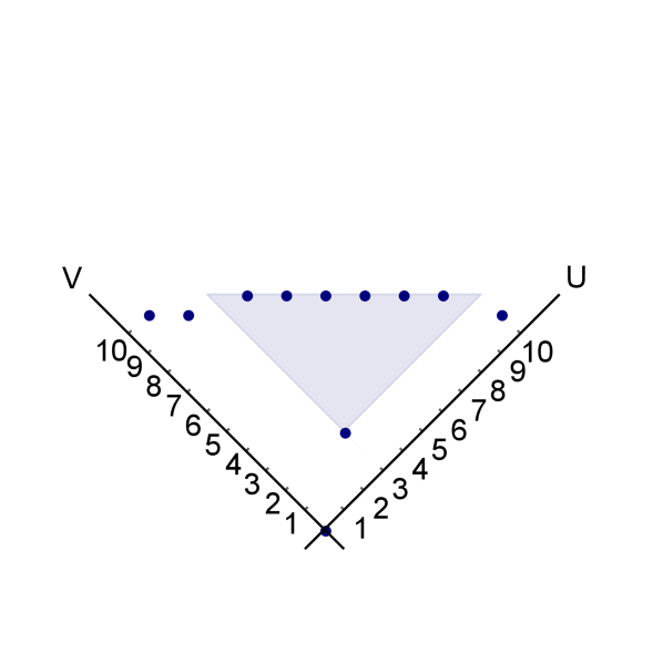
Figure 2: Illustration of a $N-2$ dimensional configuration. The future of the bulk element is shaded.

Hence $\mu_{l}=(N-1-l)$. The expression for $\Psi_{0}(N-2)$ is then easily evaluated since it involves sums over a geometric series and their derivatives

$$\Psi_{0}(N-2)=\frac{Ae^{-\beta(R-Q)}}{(1-e^{\beta Q})^{2}}\biggl{(}N-2-(N-1)e^{\beta Q}+e^{\beta Q(N-1)}\biggr{)}$$ (8)

where $Q=4\epsilon^{2}(1-3\epsilon)$ and $R$ is given as in (7).

$\mathbf{p=3:}$ This calculation is more involved. For one, the bulk elements $e_{1},e_{2}$ can form (a) an antichain or (b) a chain. These possibilities are shown in Figure 3 . In both cases we will denote the future of the $e_{1,2}$ in $\mathcal{A}_{f}$ as $F_{1,2}$ and let $l_{1,2}=|F_{1,2}|$.

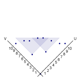
(a) Antichain with overlapping futures

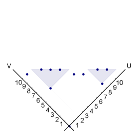
(b) Antichain with non-intersecting futures

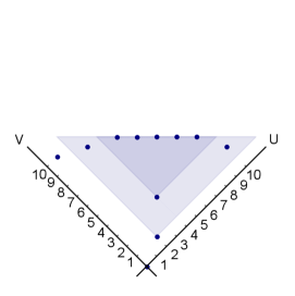
(c) Chain

Figure 3: Illustration of the three types of configuration possible with $2$ bulk elements. The future of the bulk elements is shaded.

For (a) there are two possibilities, (i) $F_{1}\cap F_{2}\neq 0$ so that $|F_{1}\cap F_{2}|=m\leq max(l_{1},l_{2})$ and (ii) $F_{1}\cap F_{2}=0$ with a “spacing” $\widetilde{m}$ between the maximum $u$ values in $F_{1}$ and the minimum $u$ value in $F_{2}$. This spacing comes from the fact that the $u$ and $v$ values in $F_{1,2}$ are contiguous as we saw for the $\mathcal{A}_{f}=N-2$ case. For (i) the non-zero abundances of order intervals are $N_{1}=N-1-m$, $N_{2}=l_{1}+l_{2}-2m$ and $N_{3}=m$ and for (ii) $N_{1}=N-1$, $N_{2}=l_{1}+l_{2}$ and $N_{3}=0$. These can be combined to case (i) since in case (ii) $m=0$.

Next, we calculate the multiplicity $\mu_{l_{1},l_{2},m,\widetilde{m}}$. In both cases (i) and (ii) the arguments in the $\mathcal{A}_{f}=N-2$ case can be used to see that $u_{1}\in[1,\ldots,N-1-l_{1}],v_{1}=N-l_{1}-u_{1}$ and $u_{2}\in[1,\ldots,N-1-l_{2}],v_{2}=N-l_{2}-u_{2}$ independently. Assume $u_{1}\prec u_{2}$. Then the contiguous values of $u$ in $F_{1}$ and $F_{2}$ are therefore such that the minimum value $u_{j_{1}}^{(1)}$ in $F_{1}$ is less than or equal to the minimum value $u_{j_{1}}^{(2)}$ in $F_{2}$. If $u_{s_{r}}^{(1)}$ denote the values of $u$ in $\mathcal{A}_{f}\backslash F_{1}$ with $r=1,\ldots,|\mathcal{A}_{f}\backslash F_{1}|$ one has the ordering

$$u_{s_{1}}^{(1)}<u_{s_{2}}^{(1)}<\ldots u_{s_{p}}^{(1)}<u_{j_{1}}^{(1)}<u_{j_{2}}^{(1)}\ldots u_{j_{l_{1}}}^{(1)}<u_{s_{p+1}}^{(1)}<\ldots u_{s_{k}}^{(1)}$$ (9)

where $k=N-3-l_{1}$. Similarly, if $u_{s_{r}}^{(2)}$ denote the values of $u$ in $\mathcal{A}_{f}\backslash F_{2}$ with $r=1,\ldots,|\mathcal{A}_{f}\backslash F_{2}|$ one has the ordering

$$u_{s_{1}}^{(2)}<u_{s_{2}}^{(2)}<\ldots u_{s_{q}}^{(2)}<u_{j_{1}}^{(2)}<u_{j_{2}}^{(2)}\ldots u_{j_{l_{2}}}^{(2)}<u_{s_{q+1}}^{(2)}<\ldots u_{s_{k}}^{(2)}$$ (10)

where now $k=N-3-l_{2}$. Since the only $u$ values below $u_{1}$ apart from $u=0$ must belong to $\mathcal{A}_{f}\backslash F_{1}$, $p=u_{1}-1$, and the only $u$ values below $u_{2}$ apart from $u=0$ and $u_{1}$ must belong to $\mathcal{A}_{f}\backslash F_{1}$, $q=u_{2}-2$ so that $p<q+1$.

For (i) with $m>0$ and $\widetilde{m}=0$, we see that $q=p+l_{1}-m$ so that $u_{2}=u_{1}+l_{1}-m+1$. For (ii) with $m=0,\widetilde{m}\geq 0$, $q=p+l_{1}+\widetilde{m}$ or $u_{2}=u_{1}+l_{1}+\widetilde{m}+1$. In other words, given $u_{1}$, $u_{2}$ is fixed to $u_{2}=u_{1}+l_{1}-m+\widetilde{m}+1$ which covers both (i) and (ii). This relationship moreover constrains the maximum value of $u_{1}$ to $N-1-l_{2}-l_{1}+m-\widetilde{m}-1$. As in the case of $\mathcal{A}_{f}=N-2$, there is no more freedom remaining: specification of $u_{1}$ (along with $l_{1,2},m,\widetilde{m}$ determines the $u$ and $v$ values of the other elements uniquely. Thus $\mu_{l_{1},l_{2},m,\widetilde{m}}=(N-2-l_{1}-l_{2}-m+\widetilde{m})$. Note that the case $u_{1}>u_{2}$ is simply an automorphism (since the bulk elements form an antichain) and hence does not contribute another factor of $\mu_{l_{1},l_{2},m,\widetilde{m}}$. Thus $\Psi^{(a)}_{0}(N-3)$ for (i) and (ii) reduce to the sums

$$\Psi^{(a,i)}_{0}(N-3) = Ae^{-\beta R}\sum_{l_{1}=1}^{N-3}\sum_{l_{2}=1}^{N-3}\sum_{m=m_{0}}^{m_{f}}(N-2-l_{1}-l_{2}+m)e^{\beta Pm}e^{\beta Q(l_{1}+l_{2})}$$

$$\Psi^{(a,ii)}_{0}(N-3) = Ae^{-\beta R}\sum_{l_{1}=1}^{(N-3-1)}\sum_{l_{2}=1}^{(N-3-l_{1})}\sum_{\widetilde{m}=0}^{(N-3-l_{1}-l_{2})}(N-2-l_{1}-l_{2}-\widetilde{m})e^{\beta Q(l_{1}+l_{2})},$$

where $P=24\epsilon^{4}$ and the limits for $m$ are $m_{0}=max(1,l_{1}+l_{2}-N+3)$ and $m_{f}=min(l_{1},l_{2})$. While these sums are straightforward to calculate, their closed form expressions are rather lengthy.

For (b) let $e_{1}\prec e_{2}$ denote the elements in the chain. In this case, $F_{2}\subseteq F_{1}\subseteq\mathcal{A}_{f}$. Here the abundance of the inclusive intervals is $N_{1}=N-1$, $N_{2}=l_{1}+1$ and $N_{3}=l_{2}$. Since the set of future elements of $e_{1}$ is $F_{1}\cup e_{2}$, and thus of cardinality $l_{1}+1$, $u_{1}\in[1,\ldots,N-2-l_{1}]$, and $v_{1}\in[1,\ldots,N-2-l_{1}]$. An argument similar to the $\mathcal{A}_{f}=N-2$ case shows that $v_{1}=N-l_{1}-u_{1}-1$. Since the future of $e_{2}$ is just $F_{2}$ and $e_{1}\prec e_{2}$, $u_{2}\in[u_{1}+1,\ldots N-l_{2}-1]$ and $v_{2}=N-l_{2}-u_{2}+1$. Since $v_{2}>v_{1}$ this means that $u_{2}<u_{1}+l_{1}-l_{2}+2$ or $u_{2}\in[u_{1}+1,\ldots,u_{1}+l_{1}-l_{2}+1]$. Therefore the multiplicity $\mu_{l_{1},l_{2}}=(l_{1}-l_{2}+1)(N-2-l_{1})$ and

$$\Psi^{(b)}_{0}(N-3)=Ae^{-\beta(R-Q)}\sum_{l_{1}=1}^{(N-3)}\sum_{l_{2}=1}^{l_{1}}(l_{1}-l_{2}+1)(N-2-l_{1})e^{\beta Ql_{1}}e^{\beta Tl_{2}}$$ (11)

where $T=4\epsilon^{2}(1-6\epsilon+6\epsilon^{2})$. Again, this is straightforward to evaluate.

As is evident from this calculation, as $p$ increases, the number of distinct configurations in the bulk increases and hence calculating the multiplicity and then $\Psi_{0}({\mathcal{N}}_{f})$ becomes rapidly more complicated. Instead, following [12] we now use Markov Chain Monte Carlo(MCMC) methods to generate the averaged action $\langle{\mathcal{S}}_{\mathrm{2d}}\rangle_{\beta}({\mathcal{N}}_{f})$ from the equilibrium partition function and additional numerical tools to obtain $\Psi_{0}(\mathcal{A})$.

3.2 Numerical Calculations

As in [12] $\langle{\mathcal{S}}_{\mathrm{2d}}\rangle_{\beta}({\mathcal{N}}_{f})$ is obtained from MCMC simulations using a module in the Cactus framework [21]. Starting from an arbitrary 2d order $U\cap V$, the Markov move consists of picking a distinct pair of elements from $U$ (or $V$) at random and exchanging them. This gives a new 2d order which we reject immediately if ${\mathcal{N}}_{f}$ is changed. If ${\mathcal{N}}_{f}$ is unchanged, on the other hand, the new 2d order is accepted or rejected according to the Metropolis-Hastings algorithm for detailed balance using the relative weights $\exp(-\beta S_{\beta}({\mathcal{N}}_{f}))$ of the initial and final causal sets. Using various observables including the action itself, this process is seen to thermalise fairly rapidly for most values of ${\mathcal{N}}_{f}$. From the thermalised ensemble, the average of the action $\langle{\mathcal{S}}_{\mathrm{2d}}\rangle_{\beta}({\mathcal{N}}_{f})$ is obtained. In order to calculate

$$\Psi_{0}({\mathcal{N}}_{f})=A{\mathcal{Z}}_{\beta}({\mathcal{N}}_{f})=A{\mathcal{Z}}_{0}({\mathcal{N}}_{f})\exp({-\int_{0}^{\beta}d\beta^{\prime}\langle{\mathcal{S}}_{\mathrm{2d}}\rangle_{\beta^{\prime}}({\mathcal{N}}_{f})})$$ (12)

it is therefore also necessary to obtain the partition function ${\mathcal{Z}}_{0}({\mathcal{N}}_{f})$ at $\beta=0$, and perform the above numerical integration of $\langle{\mathcal{S}}_{\mathrm{2d}}\rangle_{\beta^{\prime}}({\mathcal{N}}_{f})$ over $\beta^{\prime}$.

We restrict our discussions to simulations for $N=50$ element 2d orders, with $\epsilon=0.12,0.5,1.0$. Less extensive simulations for different $N$ suggest that these results are robust. Indeed, the interplay between $N,\beta,\epsilon$ gives rise to a non-trivial scaling behaviour when ${\mathcal{N}}_{i,f}$ is unrestricted, indicative of a well defined asymptotic limit [14]. We expect the same to be true for fixed ${\mathcal{N}}_{i,f}$ but a discussion of this is beyond the scope of the current work.

3.2.1 Calculating $\mathcal{Z}_{0}$

The partition function ${\mathcal{Z}}_{0}$ with no restrictions on ${\mathcal{N}}_{i,f}$ can be written as ${\mathcal{Z}}_{0}=\!\sum_{{\mathcal{N}}_{f}}{\mathcal{Z}}_{0}({\mathcal{N}}_{f})$, where ${\mathcal{Z}}_{0}({\mathcal{N}}_{f})$ is the restricted partition function. Since ${\mathcal{Z}}_{0}$ is dominated by 2d random orders ${\mathcal{Z}}_{0}({\mathcal{N}}_{f})$ is given (up to overall normalisation) by the frequency of those with fixed ${\mathcal{N}}_{f}$ from an ensemble of 2d random orders. We simulate $1.138\times 10^{10}$ 2d random orders to generate this frequency profile for ${\mathcal{N}}_{f}$ up to $19$ and find

$$\begin{array}[]{rr}N_{f}&\text{No of occurrences}\\ 1&2.32246\times 10^{8}\\ 2&1.03553\times 10^{9}\\ 3&2.12\times 10^{9}\\ 4&2.68325\times 10^{9}\\ 5&2.37839\times 10^{9}\\ 6&1.58286\times 10^{9}\\ 7&8.27049\times 10^{8}\\ 8&3.50007\times 10^{8}\\ 9&1.22738\times 10^{8}\\ 10&3.62907\times 10^{7}\\ 11&9.1807\times 10^{6}\\ 12&2.00639\times 10^{6}\\ 13&383502.\\ 14&63963.\\ 15&9483.\\ 16&1191.\\ 17&146.\\ 18&22.\\ 19&3.\\ \end{array}$$

Despite the large number of trials we only found an $N_{f}=19$ causet three times and no causet with larger $N_{f}$. This shows how much entropy disfavors these states. Beyond this the frequency becomes numerically insignificant.

Next, we use these data points together with the analytic results for $N_{f}=47,48,49$ to fit a function for ${\mathcal{Z}}_{0}({\mathcal{N}}_{f})$. The best fit estimate is shown in Figure 4.

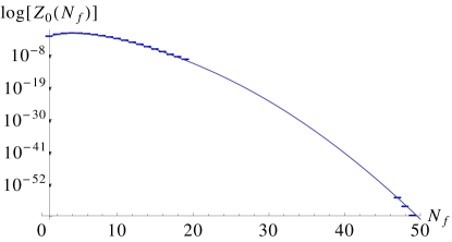
Figure 4: A log plot of the histogram for ${\mathcal{N}}_{f}$ using $1.138\times 10^{10}$ random 2d orders.

The fit function is determined by best guess as

$$(a+hx^{m}+(e+fx+gx^{2}+jx^{3}+kx^{5.5})\ln(x))e^{-b(x+d)^{2})}$$ (13)

The large number of free parameters is not important, since we only need a function that generates a good estimate of the values. The fit works very well and the error bands on it, as determined by Mathematica, are so small that we have difficulty in showing them in a plot. The plot Figure 5(b) shows that the errors are visible in the lower right corner only. Since the small error might seem an effect of the log plot and the choice of region we zoom into the peak of the distribution in a non-log plot Figure 5(a). To see the very small errors, we include Figure 5(c), which shows the difference between the estimate for ${\mathcal{Z}}_{0}({\mathcal{N}}_{f})$ and the real values together with the uncertainty on the estimate. The quality of the estimate is therefore very good and we use it as the function ${\mathcal{Z}}_{0}({\mathcal{N}}_{f})$ for the remaining part of the analysis.

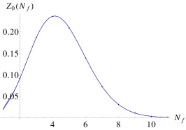
(a) Peak region

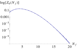
(b) Error bands

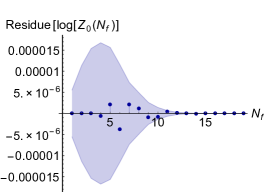
(c) Difference to bounds and residue

Figure 5: These plots illustrate the fitting for ${\mathcal{Z}}_{0}({\mathcal{N}}_{f})$. In Figure a) Zoom of best fit to ${\mathcal{Z}}_{0}({\mathcal{N}}_{f})$ with $90\%$ confidence bands. Only the peak region is shown, on a non-log scale. Figure b) is the best fit to ${\mathcal{Z}}_{0}({\mathcal{N}}_{f})$ with $90\%$ confidence bands. The errors are very small and only visible in the lower right corner. In Figure c) the dots are the difference between the calculated value for Z 0 (N f ) and the measured value, while the blue shaded region shows the upper and lower bounds for the estimate.

3.2.2 MCMC simulations

For the MCMC simulations we define a sweep as $\binom{N}{2}$ moves, and perform $10,000$ sweeps for ${\mathcal{N}}_{f}=1,\dots 46$. To compare with the best data in [12] the $\epsilon=0.12$ trials are done in finer steps of $\beta$ and coarser steps for $\epsilon=0.5,1$. In all three cases, the qualitative features observed are the same. Since thermalisation problems set in at different values of $\beta$ for different $\epsilon$, for $\epsilon=0.5,1$, the data, though coarser, spans more of the $\beta>\beta_{c}$ regime. Our conclusions take all this data into account. Analytic results are used for ${\mathcal{N}}_{f}=47,48,49$. Thermalisation typically occurs very quickly, an example of which is given in Fig (6). We give a more detailed picture of the thermalisation below

Tests of thermalisation
To ensure that our simulations thermalise we start from different bulk configurations that lie between the initial and final antichain.

• a total chain

• a total antichain

• a random 2d order

• a crystalline order

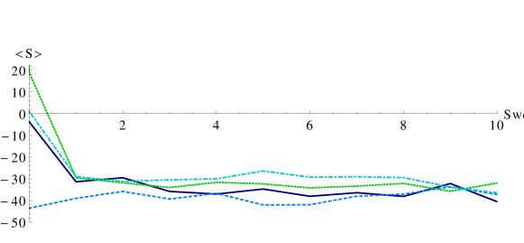
(a) Thermalisation for ${\mathcal{N}}_{f}=15$, $\beta=1$, $\epsilon=0.12$.

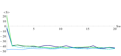
(b) Average action starting from different configurations for $\beta=7.6$ $N_{f}=27$

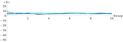
(c) Average action starting from different configurations for $\beta=6.8$ $N_{f}=45$

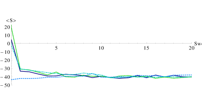
(d) Average action starting from different configurations $\beta=6$ $N_{f}=30$

(e) Average action starting from different configurations $\beta=4$ $N_{f}=30$

Figure 6: Starting from different initial configurations thermalisation is reached quickly.

Our code also allows us to start the simulations from a given configuration in a file. This makes it possible to resume simulations in a thermalised state, or test the thermalisation of special configurations. To test the thermalisation of the configurations used in our analysis we ran the code starting from different initial conditions for the three values of $\epsilon$ varying over $\beta$. We deemed the thermalisation to be sufficient if the average action for the different initial configurations agreed to within the error bars.

We found that thermalisation properties are fairly good. For $50$ element causets the configuration thermalises after few moves, independent of the length of the final chain, for smaller values of $\beta$, but gets slower as $\beta$ increases. In Figure 6 we show the thermalisation for some examples of large $\beta$ and moderately to large $N_{f}$. These configurations are those that might have had the most problems with thermalisation. Yet, as shown here, they in fact thermalise very fast.

Results of MCMC simulations
The ${\mathcal{N}}_{f}$ dependence of the phase transition is shown in Figure 7.

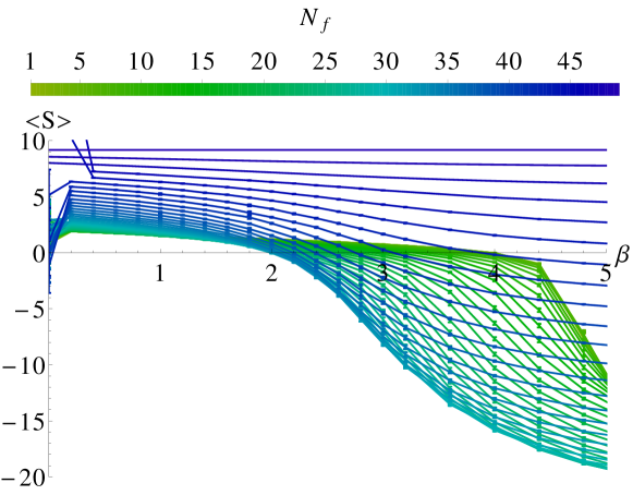
Figure 7: $\langle{\mathcal{S}}_{\mathrm{2d}}\rangle_{\beta}({\mathcal{N}}_{f})$ as a function of $\beta$, $\epsilon=0.12$.

For small values of ${\mathcal{N}}_{f}$ the behaviour of the phase transition is similar to that in [12] with a continuum phase for $\beta<\beta_{c}$ and a crystalline phase for $\beta>\beta_{c}$. As ${\mathcal{N}}_{f}$ increases the critical point $\beta_{c}$ first begins to decrease achieving a minimum value $\beta_{c}^{min}$ around ${\mathcal{N}}_{f}\sim 30$ after which it begins to increase again. For ${\mathcal{N}}_{f}>40$, the nature of the transition changes since a reduced bulk makes the two phases less distinguishable.

This rich phase structure that emerges from our calculations contains the essence of what the following analysis will extract. In particular, one can with the eye begin to see the reason for the dominance of certain configurations over others, based on the temperature at which the particular phase transition sets in.

3.2.3 Numerical Integration

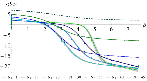
Figure 8: Errors in the interpolating functions for $\langle{\mathcal{S}}_{\mathrm{2d}}\rangle_{\beta}({\mathcal{N}}_{f})$ as a function of $\beta$, $\epsilon=0.12$.

Our MC simulations give the average action $\langle{\mathcal{S}}_{\mathrm{2d}}\rangle_{\beta}({\mathcal{N}}_{f})$. We want to numerically integrate it to find

$$\ln{\frac{{\mathcal{Z}}_{0}({\mathcal{N}}_{f})}{{\mathcal{Z}}_{\beta}({\mathcal{N}}_{f})}}=\int_{0}^{\beta}d\beta^{\prime}\langle{\mathcal{S}}_{\mathrm{2d}}\rangle_{\beta^{\prime}}({\mathcal{N}}_{f})$$ (14)

To evaluate the RHS of this equation, we begin with tabulating our measurements of $\beta$ and $\langle\mathcal{S}(\beta,\epsilon)\rangle$. We then make a best fit for this data and numerically integrate it using Mathematica. For $\epsilon=0.12$ we use the function

$$(a+f\,x)\tanh(bx+c)+d+ex$$ (15)

Using a best fit function instead of an interpolation between the points does allow us to use the additional data contained in the measurement errors of the average action. The best fit also leads to a smoother and more consistent estimate of ${\mathcal{Z}}_{\beta}({\mathcal{N}}_{f})$ compared to using a pure interpolation function. To demonstrate our method of calculation we show show the ${\mathcal{N}}_{f}=30$ case in detail. On the left hand side of Figure 9 we show $\langle{\mathcal{S}}_{\mathrm{2d}}\rangle_{\beta}({\mathcal{N}}_{f}=30)$ for $\epsilon=0.12$ together with the error bars, the fitted function and the shaded region. On the right hand side we show $-\ln{{\mathcal{Z}}_{\beta}(30)}$ calculated by integrating average action and subtracting $-\ln{{\mathcal{Z}}_{0}(30)}$. If we had approximated the average action through line segments the result for $-\ln{{\mathcal{Z}}_{\beta}(30)}$ would show jumps at the points where two line segments meet, especially at the beginning and the end of the phase transition.

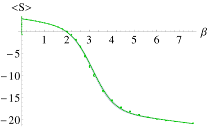
(a) $\langle\mathcal{S}(\beta,0.12)\rangle$ with best fit

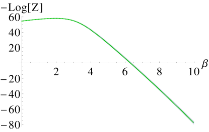
(b) $-\ln{{\mathcal{Z}}_{\beta}(30,50)}$

Figure 9: The figure on the right, $-\ln{{\mathcal{Z}}_{\beta}(30)}$ , is calculated by integrating the left hand figure,$\langle\mathcal{S}(\beta,0.12)\rangle$, and subtracting $-\ln{{\mathcal{Z}}_{0}(30)}$.

Importantly, introducing several free parameters in fitting the function is not physically significant, since the fit parameters are not themselves of independent interest.

For $\epsilon=0.5$ we need to use a different fit function

$$(a+bx)\Theta(-x+c)+d\Theta(x-c)$$ (16)

where $\Theta$ is the Heaviside step function.

3.2.4 The HH Wavefunction

Putting together the estimate of ${\mathcal{Z}}_{0}({\mathcal{N}}_{f})$ with the above results of numerical integration, we can finally normalise $\Psi_{0}({\mathcal{N}}_{f})$ using $\Sigma_{{\mathcal{N}}_{f}=1}^{N-1}|\Psi_{0}({\mathcal{N}}_{f})|^{2}=1$. This gives us $\Psi_{0}({\mathcal{N}}_{f})$ as a function of $\beta$. What is very surprising is that rather than obeying a fairly generic behaviour, $\Psi_{0}({\mathcal{N}}_{f})$ displays clear peaks about specific discrete geometries. A careful examination shows that this is a result of the rich phase structure displayed in Fig 7 and the existence of a value of ${\mathcal{N}}_{f}$ at which the critical $\beta$ is the smallest.

As $\beta$ increases, moreover, there is the interesting struggle displayed in $\Psi_{0}$ between the “entropic” component, ${\mathcal{Z}}_{0}({\mathcal{N}}_{f})$, and the action. This is shown in Figure 10 for $\epsilon=0.12,0.5$.

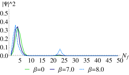
(a) $\epsilon=0.12$

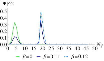
(b) $\epsilon=0.5$

Figure 10: $|\Psi_{0}({\mathcal{N}}_{f})|^{2}$ for $\epsilon=0.12,0.5$

For small $\beta$ it is dominated by the entropic contribution and is peaked around ${\mathcal{N}}_{f}\sim 4$ starting at $\beta=0$ all the way upto $\beta\sim 7.6$. Around $\beta\sim 7.0$ $|\Psi_{0}({\mathcal{N}}_{f})|^{2}$ develops a second peak at ${\mathcal{N}}_{f}\sim 23$ which gets more pronounced as $\beta$ increases. Though the thermalisation properties of the data begin to deteriorate beyond $\beta\sim 8$ there is an indication that the second peak continues to grow and the first peak shrinks. This shifting of peaks also occurs for $\epsilon=0.5$ and $\epsilon=1$; for these the second peak clearly begins to dominate the first as one goes to larger $\beta$ as shown in Figure 10. Hence it appears that as $\beta$ goes well past $\beta_{c}^{min}$ the second peak dominates the first. Importantly, the existence of well formed peaks at all $\beta$ does not arise from tweaking of parameters, but from the details of the phase transitions seen in Figure 7.

The error in $|\Psi_{0}({\mathcal{N}}_{f})|^{2}$ is estimated from the errors in the interpolating functions for $\langle{\mathcal{S}}_{\mathrm{2d}}\rangle_{\beta}({\mathcal{N}}_{f})$ and ${\mathcal{Z}}_{0}({\mathcal{N}}_{f})$ as shown in Figure 12 for $\epsilon=0.12,0.5$. The shaded region is the confidence interval for a confidence level of $95\%$ in our approximating function for $\langle{\mathcal{S}}_{\mathrm{2d}}\rangle_{\beta}({\mathcal{N}}_{f})$. The green region is the difference between the lower limit of the error in $\langle{\mathcal{S}}_{\mathrm{2d}}\rangle_{\beta}({\mathcal{N}}_{f})$ and the mean while the blue region is the difference between the upper limit in this error and the mean. Thus, there is a growth of the error around the phase transition since the lower limit begins the phase transition earlier than the upper limit. For $\epsilon=0.12$ the appearance of the second peak in lower limit, green in Figure 12, coincides with the thermalisation limit. In this case it does look as though the second peak is dominated by the error. On the other hand, it is important to note that the peak does start to develop in the lower limit as well. We show this in Figure 12, where we have zoomed in to the peak of $|\Psi_{0}|^{2}$ for $\beta=7.5$ and $\beta=8.5$ . Here, even the lower limit slowly forms a peak. For $\epsilon=0.5$ the thermalisation limit occurs at a larger $\beta$ compared to the appearance of the second peak and the errors become small enough post the phase transition, to see the dominance of the second peak. Similar analysis for the confidence region for ${\mathcal{Z}}_{0}({\mathcal{N}}_{f})$ shows the error to be subleading compared to the uncertainty in the approximation of the average action.

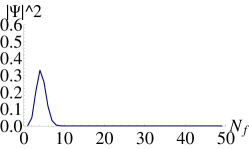
(a) $\beta=0$

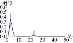
(b) $\beta=7.5,\epsilon=0.12$

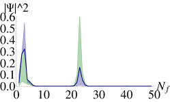
(c) $\beta=8.5,\epsilon=0.12$

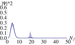
(d) $\beta=0.10,\epsilon=0.5$

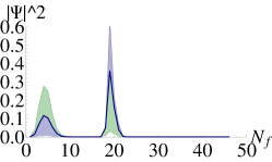
(e) $\beta=0.11,\epsilon=0.5$

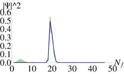
(f) $\beta=0.12,\epsilon=0.5$

Figure 11: The error in $|\Psi_{0}({\mathcal{N}}_{f})|^{2}(\beta)$ for $\epsilon=0.12,0.5$.

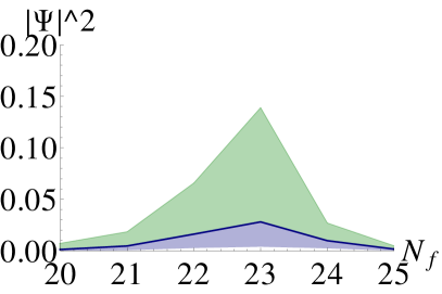
(a) $\beta=7.5,\epsilon=0.12$

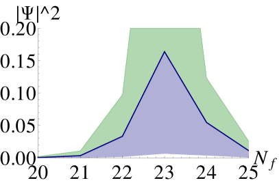
(b) $\beta=8.5,\epsilon=0.12$

Figure 12: Close up of the peak at high $\beta$ to show that the peak also forms for the lower limit in the error.

4 Results

The two different peaks in $|\Psi_{0}({\mathcal{N}}_{f})|^{2}$ correspond to two distinct discrete geometries as we will see below. Not surprisingly, these geometries strongly resemble the two phases exhibited in [12]. The first peak at smaller $\beta$ corresponds to a a continuum phase and the second peak at larger $\beta$ corresponds to a non-continuum phase with a distinctive layered structure characteristic of the crystalline phase of [12].

After locating the first and second peak values of $\beta$ and ${\mathcal{N}}_{f}$, we performed more extensive MCMC simulations for a range of observables around these peaks for $\epsilon=0.12$. They include the proper-time or height of the 2d order, the distribution of the $N_{i}$ and the ordering fraction (the ratio of the number of relations to the number of possible relations $\binom{N}{2}$.) The causets in the first peak around ${\mathcal{N}}_{f}\sim 4$ are, predictably, those which are approximated by 2d Minkowski spacetime, i.e., they are random 2d orders. Figure 13(a) is an example of a typical causet in this peak. In particular, the distribution of the $N_{i}$ is the same as that of 2-d flat spacetime [22], , and the ordering fraction gives a Myrheim-Myer dimension of 2. The distribution of the $N_{i}$ are shown by the green dots in Figure 14 which clearly follow those obtained from analytic calculations.

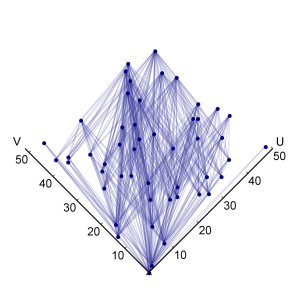
(a) ${\mathcal{N}}_{f}=4$, $\beta=0.2$

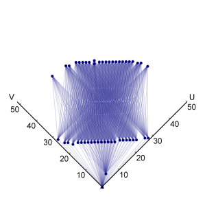
(b) ${\mathcal{N}}_{f}=23$, $\beta=7.6$

Figure 13: Typical 2d orders at $\epsilon=0.12$ associated with (a) the first and (b) the second peak, in lightcone coordinates. The lines indicate causal relations between elements.

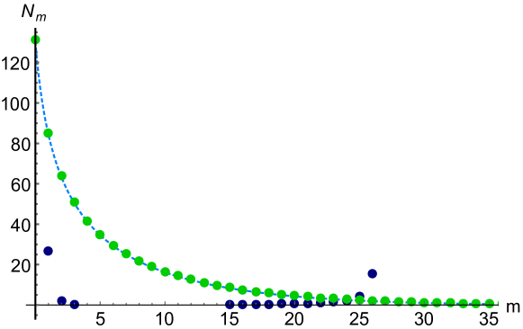
Figure 14: The green dots show $N_{i}$ for a causet in the first peak, for ${\mathcal{N}}_{f}=4,\beta=0.2$ and the blue dots for a causet from the second peak ${\mathcal{N}}_{f}=23,\beta=7.6$. The dotted line is the analytic calculation for sprinklings into 2d Minkowski spacetime. Note: $N_{0}$ for the second peak geometry is $\sim 600$ and is not visible in this plot.

The causets in the second-peak with ${\mathcal{N}}_{f}\sim 23$ share many of the features of the crystalline phase of [12]. Figure 13(b) shows a 2d order generated at the end of the MCMC trial for $N_{f}=23,\beta=7.6$. In particular, they are non-manifold like as seen in the distribution of the $N_{i}$ (the blue dots) in Figure 14. The length of the longest chain (height) in these causets is small with $h\sim 4$, while the bulk elements preferentially arrange themselves into a large antichain of size $\sim{\mathcal{N}}_{f}$. Since the free parameter $\beta$ has a ready interpretation as an inverse temperature as in the Euclidean path integral, the dominance at large $\beta$ of the non-continuum causets thus could be taken to mean that they represent the ground state of the theory. Indeed, what is surprising is that though these causets have no continuum counterpart, they nevertheless possess properties that have a ready physical interpretation of particular significance to the observable universe.

The ratio of ${\mathcal{N}}_{f}$ to the height of the poset at the second peak is $\sim 6$ which means that there is a rapid expansion from a single initial element to a large final antichain. A quick look at a first peak causet shown in Figure 13(a) shows that this ratio is less than one for causets in the first peak. In Table 1 the ratio of ${\mathcal{N}}_{f}$ to the height of the poset is shown for ${\mathcal{N}}_{f}=22,23,24$ in the second peak.

Table 1: A table of the ${\mathcal{N}}_{f}/\mathrm{Height}$ for 2d orders around the second-peak at ${\mathcal{N}}_{f}=23$ for $\epsilon=0.12$.

$\beta$	${\mathcal{N}}_{f}=22$	${\mathcal{N}}_{f}=23$	${\mathcal{N}}_{f}=24$
$6.8$	$4.53\pm 0.03$	$5.09\pm 0.03$	$5.71\pm 0.03$
$7.2$	$4.58\pm 0.02$	$5.26\pm 0.03$	$5.78\pm 0.03$
$7.6$	$4.71\pm 0.02$	$5.93\pm 0.03$	$5.95\pm 0.04$

A look at Figure 13(b) shows this explicitly: most of the elements in $\mathcal{A}_{f}$ are just $3$ time steps away from the initial element. Thus, despite being spatially large (${\mathcal{N}}_{f}\sim N/2$), the universe is still very young.

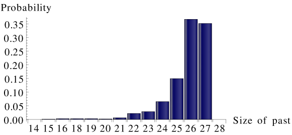
Figure 15: The average distribution of past volumes of elements in $\mathcal{A}_{f}$, for ${\mathcal{N}}_{f}=23$, $\beta=7.6$ and $\epsilon=0.12$.

Next, Figure 15 shows the probability distribution of the cardinality of the past of the elements of $\mathcal{A}_{f}$ at the second peak, averaged over a sample of $50$ 2d orders in the ensemble. The distribution is peaked around a past volume of $\sim 26$, falling off rapidly for smaller volumes. Since the number of elements in the bulk of such causets is $26$ (excluding the initial element) this means that there is a high degree of overlap in the pasts of each of the elements in $\mathcal{A}_{f}$ or high graph connectivity, given the constraints on ${\mathcal{N}}_{i,f}$. This is clearly illustrated in Figure 13.

Taking these features together we find that an initial behaviour of the universe which has much in common with our expectations of the nature of the initial conditions coming from the observable universe. This is particularly striking since the causets in the second peak are non-continuum like and have no continuum counterpart. Each causet exhibits extensive past causal contact between the elements of the final antichain, which is in stark contrast with the causal structure of the standard FRW universe. This provides a discrete alternative to continuum inflationary scenarios. While the restriction to 2d is clearly unphysical, as in other approaches one hopes to learn general lessons from it. Thus 2d CST explicitly demonstrates that the continuum may be inadequate to describe deep quantum gravity effects which could nevertheless play a crucial role in observable aspects of the early universe.

It is useful to try to compare these results with the HH wavefunction in (a) Euclidean and (b) Causal Dynamical Triangulations 2d quantum gravity [2, 3], (the latter incorporates causality, although is not fundamentally discrete) where the size of the final hypersurface is represented by the length $L$ of the boundary circle. In (a) the wavefunction has a singularity at $L=0$ but dies out exponentially with increasing $L$. The singularity can be attributed to the proliferation of baby universes when the cut-off is taken to zero [3]. In (b) while the singularity is tamed the contribution nevertheless peaks at $L=0$ with a similar large $L$ behaviour. This is in contrast with our results.

We conclude this section with some open questions and future directions.

The role played by $\beta$ in our analysis though non-trivial requires understanding. In full 2d quantum gravity $\beta$ is taken to be a Wick rotation parameter with $\beta\rightarrow-i\beta$ being the physically relevant quantum regime. Calculations with the Euclidean measure are assumed to analytically continue to this quantum regime in a manner similar to quantum field theory. In contrast, since the HH wavefunction is defined as a Euclidean path integral there is no essential need for a $\beta$ different from $1$ – all it provides is an overall scaling of the action. While in higher dimensions $\beta$ can be absorbed into rescaling of $l_{p}$ this is not the case in 2d quantum gravity because of the absence of a fundamental scale. However, our analysis clearly demonstrates that $\beta$ plays a physical role – tuning $\beta$ shifts the peak contributions from manifold like causets to non-manifold like causets. Recent work on the scaling properties of 2d CST shows that both $\beta$ and $\epsilon$ play a significant role in the large $N$ behaviour of the theory, and it is plausible that a better understanding of $\beta$ lies in this direction [14]. A similar analysis for the HH-wavefunction by adding a parameter ${\mathcal{N}}_{f}$ to the analysis (which would require much more extensive computational resources) could change the RG flows of [14] non-trivially, and lead to different fixed points for $\beta$. This is a direction we hope to pursue in the near future.

Finally, the boundary term plays a crucial role in continuum formulations of quantum gravity. It would be interesting to see how our results are affected by the recent proposal for a discrete Gibbons Hawking term [23].

5 Discussion

We now return to the question of whether $\Psi_{0}({\mathcal{N}}_{f})$ can be given a covariant interpretation in the sum-over-histories framework. We find that such an interpretation is indeed possible in the quantum measure formulation [18].

We use the more familiar (but less concrete) language of the continuum to illustrate our proposal. In the continuum the HH proposal is supposed to give the amplitude for a spatial initial condition $\Psi_{0}(\Sigma,h)$. If the subsequent evolution occurs via a putative Hamiltonian dynamics with $(\Sigma,h)$ a Cauchy hypersurface, any subsequent evolution is constrained to depending only on the initial data on $\Sigma$. However, the transition from a formulation based on the path integral with possible topology change to one that is purely Hamiltonian is somewhat an ad hoc hybrid approach. Instead, it is better to focus purely on the sum-over-histories framework. Here, the no-boundary condition requires only that the path integral is over histories with no initial boundary i.e., those that are topologically closed to the past. In particular (unless ad-hoc restrictions on topology are imposed) it is possible that initially disconnected regions of spacetime could merge, thus rendering insignificant the role of a particular “final” boundary $(\Sigma,h)$. Figure 16 shows two possible evolutions, (b) and (c), of a no-boundary spacetime (a).

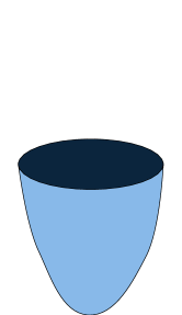
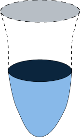
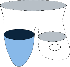
Figure 16: Two possible subsequent evolutions (b) and (c) of an initial no-boundary spacetime (a).

This illustrates the fact that further conditions on the future evolution of the histories need to be imposed if $\Psi_{0}(\Sigma,h)$ is meant to give information about the “initial” conditions of the universe. For this $(\Sigma,h)$ must capture the “complete” information of the past.

One way of doing this is to interpret $\Psi_{0}(\Sigma,h)$ not as the amplitude of the set of no-boundary spacetimes with final boundary $(\Sigma,h)$ but of all no-boundary spacetimes $(M,g)$ containing at least one spatial hypersurface $(\Sigma,h)$ which separates $(M,g)$ into its past and future. Namely, we require that $M=J^{-}(\Sigma)\cup J^{+}(\Sigma)$ (where $J^{\pm}(S)$ denotes the causal future and past of a set $S$) and such that $J^{-}(\Sigma)\cap J^{+}(\Sigma)=\Sigma$. Since this set of histories contains no reference to a “time” label it is covariant. In the language of measure theory, this set of histories forms a covariant event with amplitude (or quantum measure) $\Psi_{0}(\Sigma,h)$ [18]. In addition, we may define a unimodular time $T=\mathrm{vol}(J^{-}(\Sigma))$ for any separating hypersurface $(\Sigma,h)$ in a no-boundary spacetime. We can then similarly interpret $\Psi_{0}(\Sigma,h,T)$ to be the amplitude of the set of histories containing a separating spatial hypersurface $(\Sigma,h)$ such that $\mathrm{vol}(J^{-}(\Sigma))=T$. This too is covariant since $T$ is unique defined.

In this continuum discussion we have side-stepped at least two important sets of questions. The first is what the set of no-boundary spacetimes is; all we have done so far is specify that they are topologically closed to the past. Should they also have finite past volumes? What are the completeness requirements on these spacetimes? The second is how a Euclidean signature spacetime can be transformed into one of Lorentzian signature. Neither of these poses a problem for CST: indeed, it is natural to consider finite element causal sets that are past finite, and moreover, since causets are intrinsically Lorentzian, our framework requires no “signature matching conditions”.

In CST, covariance is implemented via label invariance. In our analysis of 2d CST, we have chosen to count all relabelings so that the measure depends not only on the action but also on the number of relabelings of a given 2d order. This is a choice of measure or partition function(driven in part by naturalness) which does not however affect covariance, since the physical observables, including the action are purely covariant. Thus the HH wave function for a fixed $N$ is indeed covariant since it is independent of the relabelings of the 2d orders.

However, just as in the continuum there is an issue if one is to interpret the measure as being merely that of the finite $N$ element causet. If the causet evolves to a larger element causet, how should we interpret $\Psi_{0}({\mathcal{N}}_{f})$? In particular ${\mathcal{N}}_{f}$ may no longer be an inextendible antichain in the larger causet and hence $\Psi_{0}({\mathcal{N}}_{f})$ cannot be thought of as representing an initial condition. This is similar to the conundrum in the continuum case whose resolution we have sketched out. Rather than think of $\Psi_{0}({\mathcal{N}}_{f})$ as the measure on the $N$-element originary causet with a future most antichain ${\mathcal{N}}_{f}$, it will be interpreted as the measure on the set $\Omega$ of all originary countable labelled causets for which $\mathcal{A}_{f}$ is separating, i.e., $\forall C\in\Omega,\,\,C=\mathrm{Past}(\mathcal{A}_{f})\cup\mathrm{Fut}(\mathcal{A}_{f})$ and $\mathrm{Past}(\mathcal{A}_{f})\cap\mathrm{Fut}(\mathcal{A}_{f})=\mathcal{A}_{f}$. Following [16, 17], the first step is to embed the finite sample space $\Omega^{N}$ of originary $N$ element causal sets in the space $\Omega$. The analogue of our prescription in the continuum would be to find the set of all causets $C\in\Omega$ for which $\mathcal{A}_{f}$ is separating, i.e., $C=\mathrm{Past}(\mathcal{A}_{f})\cup\mathrm{Fut}(\mathcal{A}_{f})$, $\mathrm{Past}(\mathcal{A}_{f})\cap\mathrm{Fut}(\mathcal{A}_{f})=\mathcal{A}_{f}$. However, since $\Omega$ is the set of labelled causets, the question is whether such a set corresponds to a covariant observable.

Following [17] we pose this question in the language of measure theory, where one begins with the triple $(\Omega,\mathfrak{A},\mu)$. Here the event algebra $\mathfrak{A}$ over $\Omega$ is a collection of subsets of $\Omega$ closed under the finite set operations of union, complementation and intersection and includes $\Omega$ and the empty set. $\mu$ is the measure on $\mathfrak{A}$ and can be either classical or quantum. A classical measure satisfies the sum rule

$$\mu(\alpha\sqcup\beta)=\mu(\alpha)+\mu(\beta)$$ (17)

for disjoint events $\alpha,\beta$, while a quantum measure satisfies the sum rule

$$\mu(\alpha\sqcup\beta\sqcup\gamma)=\mu(\alpha\sqcup\beta)+\mu(\alpha\sqcup\gamma)+\mu(\beta\sqcup\gamma)-\mu(\alpha)-\mu(\beta)-\mu(\gamma).$$ (18)

for disjoint events $\alpha,\beta,\gamma$ [18]. The set of observables is thus simply an element of the event algebra. However, since $\Omega$ is the set of labelled causets, not all choices of an event algebra will yield covariant observables. Although a non-covariant event algebra can be quotiented to form a label independent or covariant algebra, the measure too should be chosen to be label invariant.

Following [17] we instead consider the covariant event sigma algebra $\mathfrak{R}$ over the set of unlabeled causets $\Omega_{\mathrm{cov}}$ constructed as follows. A stem $\sigma\subset C\in\Omega_{\mathrm{cov}}$ is a past-set i.e., $\mathrm{Past}(\sigma)=\sigma$ and a stem event $\alpha_{\sigma}=\{C\in\Omega_{\mathrm{cov}}|\sigma\,\,\mathrm{\,is\,\,a\,\,stem\,\,in\,\,}C\}$. A stem event is thus the set of causets that possesses a particular past set or stem. The set of the stem events generate the stem sigma algebra $\mathfrak{R}$. Thus a stem event is also an event in the set of labelled causal sets $\Omega$ but is invariant under relabellings.

Define the set $\alpha^{N}_{HH}(\mathcal{A}_{f})\subset\Omega_{\mathrm{cov}}$ as the set of causets in $\Omega_{\mathrm{cov}}$ containing an inextendable antichain $\mathcal{A}_{f}$, with $|\mathrm{Past}(\mathcal{A}_{f})|=N-{\mathcal{N}}_{f}$. $\mathcal{A}_{f}$ is separating, i.e., every element in such a causet lies either in $\mathcal{A}_{f}$, $\mathrm{Past}(\mathcal{A}_{f})\backslash\mathcal{A}_{f}$ or $\mathrm{Fut}(\mathcal{A}_{f})\backslash\mathcal{A}_{f}$. This is a covariant characterisation, and indeed, we now show that $\alpha^{N}_{HH}(\mathcal{A}_{f})$ belongs to $\mathfrak{R}$ and is therefore a covariant Hartle-Hawking (HH) event. We use arguments similar to those in the Proposition in [8].

Begin with a finite causet $c_{N}\in\Omega_{N}$ with $\mathcal{A}_{f}\subset c_{N}$ the complete set of its future most elements. Let $d_{M}$, $M>N$ be a causet in $\Omega_{M}$ such that $c_{N}$ itself is a stem in $d_{M}$, but $\mathcal{A}_{f}\subset c_{N}$ is not inextendable in $d_{M}$ – in other words, $\mathcal{A}_{f}$ does not divide $d_{M}$. It is clear that the event $stem(d_{M})$ contains causets for which $\mathcal{A}_{f}$ is not inextendable, $\mathcal{A}_{f}$ being a labelled set. Further, if we require that $|\mathrm{Past}(\mathcal{A}_{f})|=N-{\mathcal{N}}_{f}$, then $stem(d_{M})$ contains no inextendable antichain $\mathcal{A}_{f}$ of cardinality ${\mathcal{N}}_{f}$ with $|\mathrm{Past}(\mathcal{A}_{f})|=N-{\mathcal{N}}_{f}$. Let $D_{c_{N}}$ denote the set of all such $d_{M}$ associated with $c_{N}$ for arbitrary $M>N$, and define $Q_{c_{N}}=\bigcup_{d\in D_{c_{N}}}stem(d)\in\mathfrak{R}$. While, $Q_{c_{N}}\subset stem(c_{N})$, it is the complement of this set which we are interested in, since these causets contain $\mathcal{A}_{f}$ as an inextendable antichain with $|\mathrm{Past}(\mathcal{A}_{f})|=N-{\mathcal{N}}_{f}$. This set, $\Phi_{c_{N}}=stem(c_{N})\backslash Q_{c_{N}}$ is also an element of $\mathfrak{R}$.

Finally, consider the set $S_{N}$ of all possible $c_{N}\subset\Omega_{N}$ with $\mathcal{A}_{f}$ an inextendable antichain and $|\mathrm{Past}(\mathcal{A}_{f})|=N-{\mathcal{N}}_{f}$. The HH event is then the set $\alpha^{N}_{HH}(\mathcal{A}_{f})=\bigcup_{c_{N}\in S_{N}}\Phi_{c_{N}}\in\mathfrak{R}$. It is clear from this construction that $\mathcal{A}_{f}$ is indeed an inextendable, dividing antichain in any infinite element causet in this set, with $|\mathrm{Past}(\mathcal{A}_{f})|=N-{\mathcal{N}}_{f}$, thus ensuring that no disjoint universe can “join up” at a coordinate time greater than $N$.

Thus the HH event $\alpha^{N}_{HH}(\mathcal{A}_{f})$ is indeed a covariant event or observable, and we may interpret our calculation of $\Psi_{0}({\mathcal{N}}_{f})$ (Eqn (2)) as a prescription for giving the measure on this class of observables. As we have constructed it, $\Psi_{0}({\mathcal{N}}_{f})\in\mathbb{R}$. We have moreover given no further information re. the nature of the measure, i.e., whether it is quantum or classical. Thus, specifying the measure on the set of all HH-events will not suffice to give us the measure of other covariant events in $\mathfrak{R}$ some of which could also be of physical interest. Nevertheless, providing an covariant interpretation for the HH wavefunction seems a satisfying start to answering what is a very challenging set of questions in quantum gravity, namely how to determine a fully covariant initial state of the universe.

MCMC simulations were conducted on the HPC cluster at the Raman Research Institute. This work was supported in part under an agreement with Theiss Research and funded by a grant from the Foundational Questions Institute (FQXI) Fund, a donor advised fund of the Silicon Valley Community Foundation on the basis of proposal FQXi-RFP3-1346 to the Foundational Questions Institute. This work was also supported by funding from the European Research Council under the European Union’s Seventh Framework Programme (FP7/2007-2013) / ERC Grant Agreement n.306425 “Challenging General Relativity”. LG was also supported by the ERC-Advance grant 291092, “Exploring the Quantum Universe” (EQU).

References

- [1] J. B. Hartle and S. W. Hawking, “Wave function of the universe,” Physical Review D 28 no. 12, (Dec., 1983) 2960–2975. http://link.aps.org/doi/10.1103/PhysRevD.28.2960.
- [2] F. David, “Loop Equations and Nonperturbative Effects in Two-dimensional Quantum Gravity,” Mod.Phys.Lett. A5 (1990) 1019–1030.
- [3] J. Ambjorn and R. Loll, “Nonperturbative Lorentzian quantum gravity, causality and topology change,” Nucl.Phys. B536 (1998) 407–434, arXiv:hep-th/9805108 [hep-th].
- [4] L. Bombelli, J. Lee, D. Meyer, and R. Sorkin, “Space-time as a causal set,” Phys.Rev.Lett. 59 (1987) 521–524.
- [5] R. D. Sorkin, “Causal sets: Discrete gravity,” in Proceedings of the Valdivia Summer School, A. Gomberoff and D. Marolf, eds., Series of the Centro de Estudios Cientificos de Santiago). New York, Springer, 2005. gr-qc/0309009.
- [6] S. Surya, “Directions in causal set quantum gravity,” in Recent Research in Quantum Gravity, A. Dasgupta, ed. Nova Science Publishers, NY, 2013. arXiv:1103.6272.
- [7] L. Bombelli, J. Henson, and R. D. Sorkin, “Discreteness without symmetry breaking: A Theorem,” Mod.Phys.Lett. A24 (2009) 2579–2587, arXiv:gr-qc/0605006 [gr-qc].
- [8] S. A. Major, D. Rideout, and S. Surya, “Spatial hypersurfaces in causal set cosmology,” Classical and Quantum Gravity 23 no. 14, (July, 2006) 4743. http://iopscience.iop.org/0264-9381/23/14/011.
- [9] R. P. Geroch, “Topology in general relativity,” Journal of Mathematical Physics 8 no. 4, (Apr., 1967) 782–786. http://scitation.aip.org/content/aip/journal/jmp/8/4/10.1063/1.1705276.
- [10] R. D. Sorkin, “Topology change and monopole creation,” Physical Review D 33 no. 4, (Feb., 1986) 978–982. http://link.aps.org/doi/10.1103/PhysRevD.33.978.
- [11] J. Louko and R. D. Sorkin, “Complex actions in two-dimensional topology change,” Class.Quant.Grav. 14 (1997) 179–204.
- [12] S. Surya, “Evidence for the continuum in 2d causal set quantum gravity,” Classical and Quantum Gravity 29 no. 13, (July, 2012) 132001. http://iopscience.iop.org/0264-9381/29/13/132001.
- [13] D. J. Kleitman and B. L. Rothschild, “Asymptotic enumeration of partial orders on a finite set,” Transactions of the American Mathematical Society 205 (1975) 205–220. http://www.ams.org/journals/tran/1975-205-00/S0002-9947-1975-0369090-9/home.html.
- [14] L. Glaser and D. O’Connor and S. Surya, “In preparation..”.
- [15] G. Brightwell, J. Henson, and S. Surya, “A 2d model of causal set quantum gravity: the emergence of the continuum,” Classical and Quantum Gravity 25 no. 10, (May, 2008) 105025. http://iopscience.iop.org/0264-9381/25/10/105025.
- [16] D. Rideout and R. Sorkin, “A classical sequential growth dynamics for causal sets,” Phys.Rev. D61 (2000) 024002.
- [17] G. Brightwell, H. F. Dowker, R. S. Garcia, J. Henson, and R. D. Sorkin, “’observables’ in causal set cosmology,” Phys.Rev. D67 (2003) 084031.
- [18] R. D. Sorkin, “An exercise in "anhomomorphic logic",” Journal of Physics: Conference Series 67 no. 1, (May, 2007) 012018. http://iopscience.iop.org/1742-6596/67/1/012018.
- [19] D. M. Benincasa and F. Dowker, “The scalar curvature of a causal set,” Phys.Rev.Lett. 104 (2010) 181301.
- [20] F. Dowker and L. Glaser, “Causal set d’alembertians for various dimensions,” Classical and Quantum Gravity 30 no. 19, (2013) 195016. http://stacks.iop.org/0264-9381/30/i=19/a=195016.
- [21] T. Goodale, G. Allen, G. Lanfermann, J. Massó, T. Radke, E. Seidel, and J. Shalf, “The Cactus framework and toolkit: Design and applications,” in Vector and Parallel Processing — VECPAR 2002, 5th International Conference, pp. 197–227. Springer, Berlin, 2003.
- [22] L. Glaser and S. Surya, “Towards a Definition of Locality in a Manifoldlike Causal Set,” Phys.Rev. D88 no. 12, (2013) 124026, arXiv:1309.3403 [gr-qc].
- [23] M. Buck, F. Dowker, I. Jubb, and S. Surya, “Boundary terms for causal sets.” arXiv:1502.05388.
- [24] G. Gibbons and J. Hartle, “Real Tunneling Geometries and the Large Scale Topology of the Universe,” Phys.Rev. D42 (1990) 2458–2468.