Qubit dephasing due to Quasiparticle Tunneling

Abstract

We study dephasing of a superconducting qubit due to quasiparticle tunneling through a Josephson junction. While qubit decay due to tunneling processes is well understood within a golden rule approximation, pure dephasing due to BCS quasiparticles gives rise to a divergent golden rule rate. We calculate qubit dephasing due to quasiparticle tunneling beyond lowest order approximation in coupling between qubit and quasiparticles. Summing up a certain class of diagrams we show that qubit dephasing due to purely longitudinal coupling to quasiparticles leads to a dephasing $\sim\exp(-x(t))$ where $x(t)$ is not linear in time on short time scales while it tends towards a selfconsistent calculated dephasing rate for longer times.

I Introduction

Superconducting quantum circuits based on the Josephson effect are promising candidates for the realization of large scale quantum computersDevoret and Schoelkopf (2013). While early qubit designs such as the chargeBouchiat et al. (1998), fluxMooij (1999) and phase qubitMartinis et al. (2002) were relatively sensitive to environmental charge and phase fluctuations, qubits such as the transmonKoch et al. (2007) or fluxonium have overcome these issues. With the 3D implementation of the transmon, decoherence times up to almost 100$\mu$s have been demonstratedPaik et al. (2011); Rigetti et al. (2012); Sears et al. (2012) closing in on quantum error correction thresholds. Even 2D implementations of transmon qubits at the threshold of quantum error correction have been demonstratedBarends et al. (2013). With these decoherence times superconducting qubits have reached regimes where previously unobservable decoherence channels such as quasiparticle tunneling could become a relevant source of dephasing. Quasiparticles as a source of decoherence have been confirmed by several experiments that clearly demonstrate the influence of non-equilibrium quasiparticles on qubit energy relaxation either with temperature dependent measurementsMartinis et al. (2009) or with quasiparticles injected on purpose Barends et al. (2011); Lenander et al. (2011); Martinis et al. (2009); Shaw et al. (2008). Quasiparticles as an intrinsic feature of superconducting devices are of particular interest because they could provide an ultimate limit to qubit coherence times. Besides equilibrium quasiparticles which, at usual qubit operation temperature, are exponentially suppressed and contribute little to the overall quasiparticle density, there always exist non equilibrium quasiparticles close to the BCS gap. Qubit decay and frequency shifts due to those non equilibrium quasiparticles have been studied in several theoretical papers Lutchyn et al. (2005); Leppäkangas and Marthaler (2012); Catelani et al. (2011a) with golden rule calculations. Diagonal elements of a qubit’s density matrix decay to their equilibrium values with a relaxation rate that is proportional to the quasiparticle spectral density $S_{qp}(\omega)$ evaluated at the qubit frequency $\epsilon_{0}$ with decay times ranging from several micro seconds up to milliseconds depending on the qubit typeLeppäkangas and Marthaler (2012). In addition to energy relaxation with decay rate $\Gamma_{1}$ quasiparticle tunneling induces pure dephasing. The decay of off-diagonal elements of the density matrix takes the form $\rho_{10}\sim e^{-\Gamma_{1}t/2}e^{-x(t)}$ with the dephasing function $x(t)$ which in general is not linear in time. Nonetheless for noise with a regular spectral density at low frequencies and for long times one can define a pure dephasing rate $\Gamma_{2^{*}}$ and the dephasing function takes the form $x(t)=\Gamma_{2^{*}}t$. Contrary to relaxation pure dephasing is proportional to the spectral density at low frequencies and a golden rule calculation yields $\Gamma_{2^{*}}\sim S(0)$. Unfortunately, the BCS density of states leads to a spectral density that diverges logarithmically as $\omega$ tends to zero. As is known from 1/f noise, dephasing due to noise with a divergent spectral density at low frequencies produces non-linear exponential decayIthier et al. (2005). For 1/f noise the dephasing function is quadratic, $x(t)\sim bt^{2}$. Since the irregularity of the quasiparticle spectral density is only logarithmic we expect a time dependence of dephasing due to quasiparticles somewhere between the linear golden rule and the quadratic 1/f-noise result, $x(t)\sim bt^{\alpha}$ with $1\leq\alpha\leq 2$. Single quasiparticle tunneling changes the parity of the qubit state and recent experimentalRistè et al. (2013) and theoreticalCatelani (2014) works suggest that this parity change can be important for qubit decoherence even for the transmon with large ratio between Josephson and charge energy. We neglect these effects in this work which is valid for small energy splittings between physical states for the same qubit level but with different parityCatelani (2014).

In this paper we us two different approaches to estimate pure dephasing due to quasiparticle tunneling. First we use a real time diagrammatic technique to find a selfconsistent pure dephasing rate.The result is similar to the selfconsistent rate defined by CatelaniCatelani et al. (2012). This approach leads to a linear exponential decay but, as we have mentioned before, dephasing due to a divergent spectral density usually is non-exponential at short times. To calculate the non-linear behavior we sum up a certain group of diagrams for quasiparticle tunneling. With this summation we recover the results obtained for a bosonic bath coupled longitudinal to the qubit. Hence we find that we can describe dephasing due to quasiparticles with relations already established for the treatment of bosonic noiseIthier et al. (2005).

II The Model

The effective Hamiltonian of a superconducting qubit coupled to quasiparticle degrees of freedom can be split into three parts:

$$H=H_{S}+H_{R}+H_{T}.$$ (1)

Here $H_{S}$ is the effective qubit Hamiltonian that includes all coherent many-body degrees of freedom that contribute to the effective two level system. $H_{R}$ describes the free quasiparticles in the superconducting leads of the system. The last term $H_{T}$ describes quasiparticle tunneling across the Josephson junction and couples qubit and quasiparticle degrees of freedom. This coupling induces decay and dephasing in the time evolution of the qubit. In general we can distinguish two different kinds of tunneling processes: tunneling processes with energy transfer inducing transitions between qubit states and elastic processes that contribute to pure dephasing only. We neglect the change in parity due to single quasiparticle tunneling processes. For a transmon qubit, whose eigenstates are superpositions of states with even and odd parity, this treatment is valid for small energy splitting between states with different parity but belonging to the same qubit eigenstateCatelani (2014).

The distinction between qubit, free quasiparticles and tunneling may, at first glance, seem artificial as the Josephson junction, described with the same quasiparticle tunnel Hamiltonian $H_{T}$, is part of the qubit. Indeed one has to be careful to avoid double counting of tunneling processes. We will come back to this issue in more detail in section (II.1) and (II.2). In the following sections we describe the three separate parts of our full Hamiltonian (1) in more detail.

II.1 Single junction qubit

In this work we consider superconducting qubits with a single Josephson junction. In a quite general form the Hamiltonian for this type of qubit reads

$$H_{S}=E_{C}(\hat{n}-n_{g})^{2}+\frac{1}{2}E_{L}(\hat{\varphi}-\varphi_{e})^{2}-E_{J}\cos\hat{\varphi}.$$ (2)

Here $\hat{n}$ is the number operator of electrons tunneled through the junction, $E_{C}$ is the charging energy, $n_{g}$ is a tunable charge offset and $\hat{\varphi}$ the phase difference between the superconducting leads. Phase difference and charge number operator are conjugate variables with the relation $[\hat{\varphi},\hat{n}]=2i$. The inductive energy $E_{L}$ describes a qubit inside a superconducting loop with applied external flux $\varphi_{e}$ (e.g. flux- or phase-qubits). Coherent Cooper pair tunneling through the junction gives rise to the last term in the Hamiltonian. $E_{J}$ is the Josephson energy which depends on the experimental setup. The Josephson energy is obtained from second order perturbation theory in the tunnel Hamiltonian $H_{T}$. The qubits we consider live in a parameter regime with $E_{J}\gg E_{C}$, where single charge effects are negligible. In this parameter regime we can neglect effects due to parityCatelani (2014). The non-linearity of the Josephson junction plays a crucial role for the superconducting qubit because it allows to truncate the Hilbert space of the effective qubit Hamiltonian to the two lowest energy levels. The effective two level Hamiltonian for the qubit (2) in its eigenbasis reads

$$H_{S}=\frac{\epsilon_{0}}{2}\sigma_{z}$$ (3)

with energy splitting $\epsilon_{0}$ and the Pauli matrix $\sigma_{z}$. We will use this effective Hamiltonian to describe the qubit throughout this work, assuming that their occurs no transition to higher energies and that the detail of the actual realization of the qubit is not important for what follows.

II.2 Quasiparticle degrees of freedom

The Hamiltonian $H_{R}$ describes the quasiparticle degrees of freedom in the superconducting leads. We treat both leads as independent BCS superconductors:

$$H_{R}=\sum\limits_{\alpha=l,r}H_{\alpha},\qquad H_{\alpha}=\sum\limits_{k}E_{\alpha,k}\gamma_{\alpha,k\sigma}^{\dagger}\gamma_{\alpha,k\sigma}$$ (4)

$\gamma_{\alpha,k\sigma}^{(\dagger)}$ are Bogoliubov annihilation (creation) operators for quasiparticles with momentum $k$, spin $\sigma$ and energy$E_{\alpha,k}=(\xi_{\alpha,k}^{2}+\Delta_{\alpha}^{2})^{1/2}$ in lead $\alpha$. $\xi_{\alpha,k}$ is the corresponding electron energy in the normal state measured from the chemical potential. We assume identical superconductors on either side of the junction which describes the usual experimental setup. Due to the presence of hot non-equilibrium quasiparticles the quasiparticle distribution functions

$$f_{\alpha}(E_{k})=\left\langle\gamma_{\alpha,k\sigma}^{\dagger}\gamma_{\alpha,k\sigma}\right\rangle,$$ (5)

differ from equilibrium Fermi functions. High energy quasiparticle excitations decay fast to the gap, e.g. due to inelastic phonon scattering, and produce a strongly increased quasiparticle density at $E_{\alpha,k}\simeq\Delta$. Hence, the distribution function differs from a Fermi distribution only in a very narrow region above the gap. For temperatures well below the gap the distribution function decays rapidly for higher energies and $f(E_{k})\ll 1$ for $E_{k}\gtrsim\Delta$. We will assume spin independent distributions which is in general a good approximation. For some calculations we describe non-equilibrium quasiparticles with a Fermi or Boltzmann distribution at an effective temperature $T^{*}>T$, where $T$ is the base temperature.

Finally we introduce the normalized density of states

$$n(\omega)=\frac{|\omega|}{\sqrt{\omega^{2}-\Delta^{2}}}\Theta(\omega^{2}-\Delta^{2})$$ (6)

of the BCS superconductors and the quasiparticle density per spin defined as

$$n_{qp}=2N_{0}\int_{\Delta}^{\infty}dEn(E)f(E).$$ (7)

Here $N_{0}=N(0)$ is the normal state density at the Fermi energy.

II.3 Quasiparticle Tunneling

Electron tunneling

The last term in the effective Hamiltonian (1) describes electron tunneling through the junction,

$$H_{T}=t\sum\limits_{kq\sigma}e^{i\hat{\varphi}/2}c_{r,q\sigma}^{\dagger}c_{l,k\sigma}+h.c.$$ (8)

with electron creation/ annihilation operators $c_{\alpha,k\sigma}^{(\dagger)}$. The commutation relation $[\hat{n},e^{i\hat{\varphi}/2}]=1$ implies the representation $e^{i\hat{\varphi}/2}=\sum_{n}|n+1\rangle\langle n|$ for the charge transfer operator $\hat{T}\equiv e^{i\hat{\varphi}/2}$. Therefor this operator, which carries the phase information of the two superconductors, describes the charge transfer due to tunneling in the qubit’s Hilbert space for $E_{J}\gg E_{C}$. Here, we assumed a constant and real tunneling matrix element $t$ which relates to the Josephson energy as $E_{J,0}=\pi^{2}t^{2}N_{0}^{2}\Delta_{0}$. The subscripts in the Josephson energy and the gap denote equilibrium quantities at zero temperature.

Quasiparticles

For use in perturbation theory we need the tunneling Hamiltonian expressed with free particle operators. For the BCS superconductors these are Bogoliubov quasiparticles with the transformation

$$\begin{pmatrix}c_{k\uparrow}\\ c_{-k\downarrow}^{\dagger}\end{pmatrix}=\begin{pmatrix}u_{k}&-v_{k}\\ v_{k}&u_{k}\end{pmatrix}\begin{pmatrix}\gamma_{k\uparrow}\\ \gamma_{k\downarrow}^{\dagger}\end{pmatrix}$$ (9)

we find the tunneling Hamiltonian

$$H_{T}=H_{qp}+H_{p}=t\sum\limits_{kq\sigma}(A_{kq}\gamma_{q\sigma,r}^{\dagger}\gamma_{k\sigma,l}+h.c.)$$

$$+t\sum\limits_{kq\sigma}(\sigma B_{kq}\gamma_{q\sigma,r}\gamma_{k\bar{\sigma},l}+h.c.).$$ (10)

Here $u_{k}^{2}=1-v_{k}^{2}=\frac{1}{2}(1+\xi_{k}/E_{k})$ are real coefficients while the phase dependence has already been taken into account with the charge transfer operator. In the transformed Hamiltonian the first term $H_{qp}$ with coherence factor

$$A_{kk^{\prime}}=e^{i\varphi/2}u_{k,l}u_{k^{\prime},r}-e^{-i\varphi/2}v_{k,l}v_{k^{\prime},r}$$ (11)

describes single quasiparticle tunneling while the second term $H_{p}$ refers to pair tunneling processes with

$$B_{kk^{\prime}}=e^{i\varphi/2}u_{k,l}v_{k^{\prime},r}+e^{-i\varphi/2}v_{k,l}u_{k^{\prime},r}.$$ (12)

The pair Hamiltonian provides the main contribution to the Josephson term in the qubit Hamiltonian $\sim E_{J}\cos\varphi$ but does not contribute to qubit decoherence as long as relevant energies are small compared to the gap which is always the case for dephasing. On the other hand $H_{qp}$ describes single quasiparticles present in the junction region which undergo incoherent tunneling processes and ultimately induce qubit decoherence. In addition to decoherence, quasiparticles lead to corrections of the qubit energies in two waysCatelani et al. (2011a). Virtual transitions between qubit states lead to a change in energy levels. Second, quasiparticles change physical parameters of the junction. Both, $E_{J}$ and $\Delta$, change linearly with the ratio between quasiparticle and Cooper pair density $x_{qp}=n_{qp}/(2N_{0}\Delta_{0})$. The resulting corrections to the qubit energy splitting have been derived by Catelani et all.Catelani et al. (2011a). This work will focus on decoherence effects and we will assume that energy corrections to the qubit eigenstates have been included in the effective qubit Hamiltonian. For the qubits considered in this work transitions to higher levels of the effective qubit Hamiltonian are strongly suppressed due to the large Josephson energy which minimizes single charge effects. Hence we truncate the tunneling Hamiltonian to the two dimensional qubit Hilbert space according toLutchyn et al. (2005)

$$\hat{T}=\alpha I+\vec{\beta}\cdot\vec{\sigma},$$ (13)

where $I$ is the unit operator in qubit space. We find the coefficients in this expansion

$$\alpha=\frac{1}{2}(\langle 1|\hat{T}|1\rangle+\langle 0|\hat{T}|0\rangle)$$ (14)

$$\beta_{z}=\frac{1}{2}(\langle 1|\hat{T}|1\rangle-\langle 0|\hat{T}|0\rangle)$$ (15)

$$\beta_{x}=\langle 1|\hat{T}|0\rangle+\langle 0|\hat{T}|1\rangle$$ (16)

$$\beta_{y}=-i\langle 1|\hat{T}|0\rangle+i\langle 0|\hat{T}|1\rangle$$ (17)

The terms proportional to $\sigma_{x}$ and $\sigma_{y}$ induce state transitions. They describe inelastic tunneling processes with energy exchange between qubit and bath producing qubit energy relaxation. We will focus on pure dephasing taking only $\sigma_{z}$ into account and neglecting other contributions from quasiparticle tunneling such that $\hat{T}\rightarrow\beta_{z}\sigma_{z}$ and the tunneling Hamiltonian can be written as

$$H_{T} =\sigma_{z}t\sum\limits_{kq\sigma}\left[A^{z}_{kq}\gamma_{q\sigma,r}^{\dagger}\gamma_{k\sigma,l}\right.$$

$$\qquad+\left.\sigma B^{z}_{kq}\gamma_{q\sigma,r}\gamma_{k\bar{\sigma},l}+h.c.\right]$$

$$=\sigma_{z}(\hat{R}_{qp}+\hat{R}_{p})\equiv\sigma_{z}\hat{R}$$ (18)

To avoid double counting of processes that have been taken into account in $E_{J}$ already we have to add an additional term to $H_{T}$Lutchyn et al. (2005); Leppäkangas and Marthaler (2012):

$$H_{T}\rightarrow H_{T}^{\prime}=H_{T}+E_{J}\cos\varphi.$$ (19)

II.4 Spectral density

The effect of tunneling quasiparticles on the qubit is described by their spectral density, $S(t)=\langle\hat{R}(0)\hat{R}(t)\rangle$ and its Fourier transform $S(\omega)$. For the quasiparticle part $H_{qp}$ we find the spectral density

$$S_{qp}(\omega)=\frac{16}{\pi^{2}}\frac{E_{J}}{\Delta}\int\limits_{\Delta}^{\infty}\int\limits_{\Delta}^{\infty}dEdE^{\prime}\,n(E)n(E^{\prime})|A(E,E^{\prime})|^{2}$$

$$\times f(E)\left(1-f(E^{\prime})\right)\delta(\omega+E-E^{\prime})$$ (20)

$$|A(E,E^{\prime})|^{2}=|\beta_{z}|^{2}(1-\cos\vartheta\frac{\Delta^{2}}{EE^{\prime}})$$ (21)

with $\cos\vartheta=(\text{Re}[\beta_{z}]^{2}-\text{Im}[\beta_{z}]^{2})/(|\beta_{z}|^{2})$, a interference factor due to the quasiparticle-qubit interaction Leppäkangas and Marthaler (2012); Pop et al. (2014) This interference plays a crucial role because it determines whether the spectral density diverges or remains finite as $\omega\to 0$. If $\cos\vartheta=1$ the singularity due to the BCS density of states cancels out and the spectral density remains finite. For such a qubit the dephasing rate due to quasiparticle tunneling usually remains small and plays only a negligible role. Even for small deviations from $\cos\vartheta=1$ the quasiparticle spectral density is log divergent at zero frequency and it remains open whether this leads to strongly increased dephasing rates. To conclude this section we have a look at the pair Hamiltonian. It yields the spectral density

$$S_{p}(\omega)=\frac{16}{\pi^{2}}\frac{E_{J}}{\Delta}\int\limits_{\Delta}^{\infty}\int\limits_{\Delta}^{\infty}dEdE^{\prime}\,n(E)n(E^{\prime})|B(E,E^{\prime})|^{2}$$

$$\times\left\{\left(1-f(E)\right)\left(1-f(E^{\prime})\right)\delta(\omega-E-E^{\prime})\right.$$

$$+\left.f(E)f(E^{\prime})\delta(\omega+E+E^{\prime})\right\}.$$ (22)

For the pair spectral density to become finite we need at least an energy $|\omega|\gtrsim 2\Delta$. In a usual QED circuit the BCS gap is by far the largest energy scale, particularly the gap exceeds the relevant energy scale defined by the energy splitting of the qubit, $\Delta\gg\epsilon_{0}$. Therefore we can neglect the pair Hamiltonian from now on and focus on the single quasiparticle tunneling described by $H_{qp}$.

III Qubit Decoherence

The effective Hamiltonian (1) describes a small system with only a few degrees of freedom (qubit) coupled to large reservoirs (leads). Tracing out quasiparticle degrees of freedom we find the reduced density matrix $\rho(t)=\text{Tr}_{qp}\left[\varrho(t)\right]$ of the qubit. We denote the full density matrix with $\varrho(t)$ and the reduced density matrix, describing only the qubit, with $\rho(t)$. Assuming that the full density matrix factorizes at some initial time $t_{0}$, $\varrho(t_{0})=\rho(t_{0})\rho_{qp}(t_{0})$, we find an exact relation for the matrix elements $\rho_{ss^{\prime}}=\langle s|\rho|s^{\prime}\rangle$:

$$\rho_{ss^{\prime}}(t)= e^{-i(E_{s}-E_{s^{\prime}})(t-t_{0})}\sum\limits_{qq^{\prime}}\rho_{qq^{\prime}}(t_{0})$$

$$\times\text{Tr}_{qp}\left\{\langle q^{\prime}|U_{I}^{\dagger}(t,t_{0})|s^{\prime}\rangle\langle s|U_{I}(t,t_{0})|q\rangle\rho_{R}(t_{0})\right\}.$$ (23)

where $\text{Tr}_{qp}\{\dots\}$ denotes a trace with respect to quasiparticle states, $|s\rangle$ are qubit states and $U_{I}(t,t^{\prime})$ is the time evolution operator in the interaction picture

$$U_{I}(t,t_{0})=\text{Texp}\left\{-i\int\limits_{t_{0}}^{t}H_{T}(t^{\prime})dt^{\prime}\right\}.$$ (24)

Expanding the time evolution operators in equation (23) we find a real time diagrammatic series for the time evolution of the the reduced density matrix. With the time evolution superoperator $\Pi(t,t_{0})$ we can rewrite the matrix time evolution as $\rho(t)=\Pi(t-t_{0})\rho(t_{0})$ where the time evolution superoperator’s matrix elements satisfy the master equation

$$\dot{\Pi}_{ss^{\prime}\leftarrow qq^{\prime}}(t,t_{0})=i(E_{s}-E_{s^{\prime}})\Pi_{ss^{\prime}\leftarrow qq^{\prime}}(t,t_{0})$$

$$+\sum\limits_{q_{1}q_{1}^{\prime}}\int\limits_{t_{0}}^{t}\Sigma_{ss^{\prime}\leftarrow q_{1}q_{1}^{\prime}}(t,t^{\prime})\Pi_{q_{1}q_{1}^{\prime}\leftarrow qq^{\prime}}(t^{\prime},t_{0}).$$ (25)

The first term in the Master equation describes free time evolution, while the kernel $\Sigma(t,t^{\prime})$ contains all reservoir effects. In the diagrammatic language we can identify the kernel with the selfenergy, the sum of all irreducible diagrams. The diagrammatic approach to the full time evolution is quite general. However, for pure dephasing with $H_{T}=\sigma_{z}\hat{R}$ (18) the perturbation is diagonal in qubit space and we can simplify the problem. Instead of dealing with the full superoperator $\Pi_{deph}$ we can separate the free time evolution of the qubit states from the noise induced incoherent time evolution $F(t,t_{0})$ as $\Pi_{deph}(t,t_{0})=\Pi_{0}(t-t_{0})e^{\Gamma_{1}t/2}F(t-t_{0})$.The incoherent time evolution is no operator but an ordinary function. Later we will show that for quasiparticle tunneling $F(t)\sim e^{-x(t)}$ and will refer to $x(t)$ as dephasing function. From (23), it follows

$$\rho_{ss^{\prime}}(t)=e^{-i(E_{s}-E_{s^{\prime}})(t-t_{0})}\rho_{ss^{\prime}}(t_{0})F_{ss^{\prime}}(t,t_{0}).$$ (26)

with the incoherent time evolution $F_{ss^{\prime}}$ defined as

$$F_{ss^{\prime}}(t,t_{0})=\text{Tr}_{R}\left\{U_{I}^{\dagger}(t,t_{0},s^{\prime})U_{I}(t,t_{0},s)\rho_{R}(t_{0})\right\}$$ (27)

$$U_{I}(t,t_{0},s)=T\exp\left\{-is\int\limits_{t_{0}}^{t}\hat{R}(t^{\prime})dt^{\prime}\right\}$$ (28)

where $s=\pm 1$ for excited/ ground state respectively. For $s=s^{\prime}$ the two time ordered exponentials are inverse to each other so that the diagonal elements of the dephasing function equal to one. This does not come as a surprise since the diagonal elements of the density matrix do not feel the longitudinal coupling and evolve free in time. Using that the trace over odd powers of the tunneling Hamiltonian vanishes and demanding a physical density matrix, $\rho_{01}(t)=\rho_{10}^{*}(t)$, we find $F_{01}=F_{10}\equiv F(t,t_{0})$ where $F(t,t_{0})$ is a real valued function. In the following sections we will use a diagrammatic expansion to calculate $F(t)$. The standard way to obtain dephasing rates uses lowest order Markov approximation and the corresponding rate is proportional to the quasiparticle spectral density at zero energy,

$$\Gamma_{2^{*}}\sim S_{qp}(0).$$ (29)

However due to the square root divergent BCS density of states the quasiparticle spectral density has a logarithmic divergence at zero frequency and the lowest order Markovian dephasing rate is ill defined. We solve this problem with the introduction of a selfconsistent dephasing function producing a selfconsistent rate equation, similar toLutchyn et al. (2005). In the section after we calculate the dephasing function using equation (27) without diagrammatic expansion and Markov approximation. Pure dephasing is dominated by quasiparticle energies $\omega=E-\Delta\sim 0$. Equation (22) clearly shows, that the pair Hamiltonian contributes to the spectral density only at energies $\omega\gtrsim 2\Delta$. Therefore it does not contribute to pure dephasing and we focus on $H_{qp}$ from now on, neglecting pair contributions.

III.1 Diagrammatic Expansion - Self consistent rate

In this section we use a real time diagrammatic expansion to calculate the dephasing function $F(t,t_{0})$. This expansion is well established in the context of open quantum systems and we sketch only some steps that are important for our specific calculation. The first step on the way to a diagrammatic description of the problem is to expand the exponentials in (27) and represent the series on a Keldysh contour. The dephasing function is the sum of all diagrams. In order to find the master equation (25) we define the self energy $\Sigma$ in the usual way as the sum of all irreducible diagrams:

Here solid dots represent tunneling vertices, a dashed directed line is a contraction in the right lead while a directed solid line represents a contraction in the left lead and horizontal lines are free time evolution which, for the dephasing function $F$, equals to one. We restrict the series to diagrams with two vertex fermionic loops. In other words a left lead contraction between two vertices implies a right lead contraction between the same vertices. Since we assume identical superconductors the direction within each loop is unimportant and we can combine the two possible directions into one contraction between time $t$ and time $t^{\prime}$. Each of those contractions $\gamma^{\gtrless}(t-t^{\prime})$ yields the quasiparticle spectral density $S(\pm(t-t^{\prime}))$ where $\gtrless$ for $t\gtrless t^{\prime}$ with respect to the Keldysh contour. With the selfenergy we find the Dyson equation for the dephasing function $F$ which we illustrate diagrammatically

The time derivate of the Dyson equation shown above yields the master equation (27) for the dephasing function. Assuming a memoryless bath we can apply Markov approximation. For a memoryless bath it holds that the kernel $\Sigma(t)$ decays on time scales much shorter then typical qubit decay times. In this case the integration region in (25) is effectively reduced to a narrow region around $t=t^{\prime}$. The dephasing function $F(t^{\prime})$ is constant in this region and can be replaced by its value at time $t$. In this approximation quasiparticle tunneling produces an exponential decay with rate

$$\Gamma_{2^{*}}=\lim\limits_{\eta\rightarrow 0}\int\limits_{-\infty}^{0}dt\,\varSigma(t)e^{\eta t}$$ (30)

where $\eta$ ensures convergence. In first order four diagrams contribute to $\varSigma(t)$:

The first two diagrams each yield $S(t)$ while each of the remaining two yields $S(-t)$. With the Fourier transformed spectral density we find

$$\Gamma_{2^{*}}=-2\lim\limits_{\eta\rightarrow 0}\int d\omega S_{qp}(\omega)\int\limits_{0}^{\infty}dt\,e^{-\eta t}\cos\omega t$$

$$=2\pi\lim\limits_{\eta\rightarrow 0}\int d\omega S_{qp}(\omega)\frac{1}{\pi}\frac{\eta}{\omega^{2}+\eta^{2}}.$$ (31)

In the given limit the Lorentzian in the latter equation yields a delta function and we find the dephasing rate $J_{2^{*}}\sim S_{qp}(0)$. Unfortunately the spectral density defined in (20) has a logarithmic divergence for $\omega=0$. Thus the first order Markovian rate is ill defined and we need to reconsider our calculations. We want to notice that there exists an exception to this statement. A closer look on the spectral density reveals that the divergence is canceled for $\cos\vartheta=1$ which is the case for an symmetric Hamiltonian. A qubit to which this applies in good approximation is the transmon ($E_{L}=0$, $E_{J}\gg E_{C}$). In this case one finds

$$\Gamma_{2^{*}}=\frac{32|\beta_{z}|^{2}}{\pi}\frac{E_{J}}{\Delta}f(\Delta).$$ (32)

Even for the transmon the Hamiltonian $H\sim(n-n_{g})^{2}$ is not strictly symmetric due to the gate charge/ offset charge $n_{g}$. However since $E_{C}\ll E_{J}$ the influence of $n_{g}$ is exponentially small and as we will show later one can regularize the log divergence in the rate. The regularized rate is not large enough to counter the exponentially small matrix element due to the almost symmetric Hamiltonian and (32) remains the dominating contribution to the transmon dephasing rate.

III.2 Selfconsistent Born-Markov

Between vertices in the first order selfenergy a free time evolution occurs which induces no native decay into the selfenergy. However, it is possible to generate convergence by including the decay of the propagator $F(t,t^{\prime})$. This is achieved within a selfconsistent Born approximation for the selfenergy and the dephasing function $F$. We replace the free propagators in the first oder diagrams with full propagators:

Within this approximation we are able to sum up all diagrams that belong to a subclass we call ’boxed’. In this context ’boxed’ refers to all diagrams where the earliest and latest vertex (with respect to real time) are contracted, the second and second last are contracted and so forth. Some diagrams of the boxed type:

We find the self-consistent selfenergy

$$\Sigma(t)=2(S_{qp}(t)+S_{qp}(-t))F(t).$$ (33)

In Markov approximation we know the solution of the master equation (25) for the dephasing function is a simple exponential decay with rate $\Gamma_{2^{*}}$, $F(t)=\exp(-\Gamma_{2^{*}}t)$. With this ansatz for $F(t)$ and the definition (30) for the Markovian dephasing rate we find the selfconsistent dephasing rate

$$\Gamma_{2^{*}}=-2\int d\omega S_{qp}(\omega)\int\limits_{0}^{\infty}dt\,e^{-\Gamma_{2^{*}}t}\cos\omega t$$

$$=2\pi\int d\omega S_{qp}(\omega)\frac{1}{\pi}\frac{\Gamma_{2^{*}}}{\omega^{2}+\Gamma_{2^{*}}^{2}}.$$ (34)

III.3 Beyond Markov - Tunneling as bosonic noise

In this section we sum up all diagrams which include only two-vertex fermionic loops, the class of diagrams we have been using throughout this paper. We start from the definition (27) of the incoherent time evolution $F(t)$ and introduce the contour time ordering $T_{C}$ which orders operators with respect to the Keldysh contour introduced in the previous section,

$$F(t-t_{0})=\text{Tr}_{qp}\left\{T_{C}\exp\left\{i\int\limits_{t_{0}}^{t}\hat{R}(t^{\prime})dt^{\prime}\right\}\right\}.$$ (35)

with $H_{qp}=\sigma_{z}\hat{R}$. The quasiparticle operator $\hat{R}$ is defined as the single particle part in (18). We notice that this operator is bilinear in fermionic operators (though it is linear for each lead separately). In the diagrams we include in our approximation only correlations between full $\hat{R}$ operators occur. Hence the bath behaves similar to a bath linear in bosonic operators. Therefore we expect to find the same behavior as for a bosonic bath. To confirm this suspicion we expand the exponentials and use Wick’s theorem to calculate the trace over reservoir states:

$$F(t) =\sum\limits_{n=0}^{\infty}\frac{(-1)^{n}}{(2n)!}\idotsint dt_{1}\cdots dt_{2n}\langle T_{C}[\hat{R}(t_{1})\cdots\hat{R}(t_{2n})]\rangle$$

$$=\sum\limits_{n=0}^{\infty}\frac{(-1)^{n}}{(2n)!}\sum\limits_{P}\prod\limits_{\{ij\}\in P}\iint dt_{i}dt_{j}\langle T_{C}[\hat{R}(t_{i})\hat{R}(t_{j})]\rangle.$$ (36)

Here $P$ denotes all permutations of time arguments in the trace. Exchanging two operators does not produce a minus sign in this case since the bath operator $R$ is bilinear in fermionic operators. The contour ordered bath correlation function $\langle T_{C}[R(t_{i})R(t_{j})]\rangle$ is just the first order self energy and we find

$$F(t)=\exp\left[-2\int\limits_{-\infty}^{\infty}d\omega S_{qp}(\omega)\int\limits_{t_{0}}^{t}dt_{1}\int\limits_{t_{0}}^{t_{1}}dt_{2}\cos(\omega(t_{1}-t_{2}))\right]$$ (37)

This yields an exponential decay with nonlinear and time dependent dephasing ’rate’, $x_{2}(t)$, where $x_{2}(t)$ is the known dephasing function for a Ramsey experiment with bosonic noiseIthier et al. (2005):

$$x_{2}(t)=t^{2}\int d\omega S_{qp}(\omega)\text{sinc}^{2}\left(\frac{\omega t}{2}\right)$$ (38)

Experiments suggest that dephasing times due to quasiparticle tunneling are at least in the order of micro seconds while typical quasiparticle energies are of order $\Delta\sim 100$GHz. The quadratic sinc function suppresses the integrand at values $\omega t\sim\mathcal{O}(1)$. So the spectral density is evaluated at energies $\omega\sim 10^{6}/s$ which on the scale of quasiparticle energies implies $\omega\approx 0$. The largest contribution to the dephasing rate still arises from small frequencies. Since our treatment of quasiparticle tunneling is equivalent to a bosonic bath we can not only explain a Ramsey experiment, which describes off-diagonal element decay after initial preparation, with decay function (38) but any measurement protocol with different pulse sequencesBylander et al. (2011a).

IV Results

IV.1 Analytical results

In this section we calculate both selfconsistent- and non Markovian dephasing for a narrow quasi particle distribution above the gap, $f(E)\approx 0$ for $E\gtrsim\Delta$ such that the relation

$$S_{qp}(\omega)=\int\limits_{1}^{\infty}J(\omega/\Delta,x)n(x)f(x)=x_{qp}J(\omega/\Delta,1)$$ (39)

holds where $x_{qp}$ is the quasiparticle density normalized to Cooper pair density,

$$x_{qp}=\frac{1}{2\Delta N_{0}}n_{qp}=\int\limits_{1}^{\infty}f(x)n(x)$$ (40)

and $x=E/\Delta$ is the normalized quasiparticle energy. This kind of quasiparticle distribution reflects the experimental situation quite accurately. While quasiparticles may be generated even at higher energies they decay rapidly to the gap due to inelastic phonon scattering while quasiparticle recombination is rather slow compared to relaxation. This kind of processes lead to a pronounced density of quasiparticles with energy close to the gap while for higher energies the distribution is thermal. For this kind of system we find the quasiparticle spectral density

$$S_{qp}(\omega)=\frac{16E_{j}}{\pi^{2}}x_{qp}\frac{1+\omega-\cos\vartheta}{\sqrt{2\omega}}.$$ (41)

This yields the selfconsistent rate equation for the normalized dephasing rate $\gamma\equiv\Gamma_{2^{*}}/\Delta$

$$\gamma=\frac{32E_{j}}{\pi\Delta}x_{qp}\frac{1+\gamma-\cos\vartheta}{\sqrt{\gamma}}.$$ (42)

Experiments suggest that $\Gamma\lesssim 1$MHz while $\Delta\sim 10^{2}$GHz and we expect $\gamma\ll 1$. For $\cos\vartheta\neq 1$ we find:

$$\gamma\approx\left(\frac{32E_{j}x_{qp}}{\pi\Delta}(1-\cos\vartheta)\right)^{2/3}$$ (43)

while for $\cos\vartheta=1$

$$\gamma=\left(\frac{32E_{j}x_{qp}}{\pi\Delta}\right)^{2}.$$ (44)

For the approximated spectral density we find the non-Markovian dephasing function for boson like noise is given by

$$x_{2}(t)=\frac{32E_{j}x_{qp}}{\pi\Delta}\frac{1}{\sqrt{\pi}}\left[\frac{4}{3}(1-\cos\vartheta)(\Delta t)^{3/2}+2(\Delta t)^{1/2}\right].$$ (45)

For the case $\cos\vartheta=1$ we can define a rate as $x(t)\sim(\gamma_{2}\Delta t)^{1/2}$ with

$$\gamma_{2}=\frac{4}{\pi}\left[\frac{32E_{j}x_{qp}}{\pi\Delta}\right]^{2}=\frac{4}{\pi}\gamma$$ (46)

while for $\cos\vartheta\neq 1$ we find with $x(t)\sim(\gamma_{2}\Delta t)^{3/2}$ a rate

$$\gamma_{2}=\left(\frac{4}{3\sqrt{\pi}}\right)^{2/3}\left[\frac{32E_{j}x_{qp}}{\pi\Delta}(1-\cos\vartheta)\right]^{2/3}=\left(\frac{4}{3\sqrt{\pi}}\right)^{2/3}\gamma.$$ (47)

We find that the non Markovian ’rates’ as defined above are proportional to the rates obtained from the self-consistent Born approximation but with a different time dependence. It remains the question of applicability of this approximation. The basic idea behind it is a very narrow distribution function $f(x)$ with width $\Lambda=\delta E/\Delta\ll 1$. To apply the integral approximation (39) the function $S_{qp}(x)$ should not change much within the region $0\leq x\leq\Lambda$. For the quasiparticle spectral density this holds for $\omega>\Lambda$ so that the approximation works quite good for qubit decay where $\omega\sim\epsilon_{0}$. Dephasing on the other hand is dominated by frequencies $\omega\sim 0$. Especially in the long time limit the sinc function decays for frequencies in the MHz regime and $\omega\lesssim\delta E$ reflects this situation more realistically. We can estimate the time scale on which this approximation is valid for a Fermi distribution with $\mu\approx\Delta$. In this case the quasiparticle width $\Lambda$ above the gap is of order temperature, $\Lambda\sim k_{B}T$. In this case the approximation is valid for a time scale up to ($k_{B}=\hbar=1$) $t\lesssim T^{-1}$ For a temperature $T=2.3mK=0.001\Delta$ for aluminum we find that the approximation should work up to $t\approx 10^{-2}\mu s$. In Fig 1(b) we can approximately confirm this result for $\cos\vartheta\neq 1$. In general for this approximation to be valid an combination of relative slow dephasing rates and large frequencies must be fulfilled. This can hold only for short times in a typical qubit setup. For longer times, e.g. smaller frequencies, we expect that the non Markovian dephasing becomes linear in time and approaches the selfconsistent dephasing rates for $t\to\infty$. For short times the approximation reveals an interesting result since the time dependence is - as we expected - somewhere between a linear decay for a regular spectral density and a $t^{2}$ decay for $1/f$ noise, in this case $\sim t^{3/2}$. For $\cos\vartheta=1$ the spectral density tends to zero as $\omega$ approaches zero and dephasing is even slower than linear decay - $\sim t^{1/2}$ for small times. In the next section we compare the analytical result with numerical calculations of the full non Markovian dephasing. We confirm the expected behavior $x(t)\sim t^{n/2}$ with $n=2\pm 1$ for $t\ll 1\mu s$ while for $t\gtrsim\mathcal{O}(10^{-2}\mu s)$ the dephasing becomes linear.

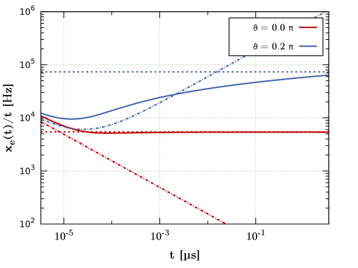
(a)

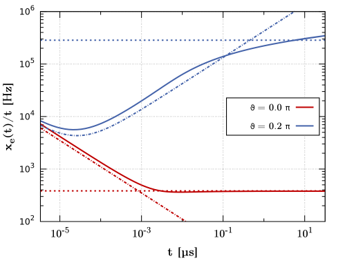
(b)

Figure 1: Normalized non Markovian dephasing function over time $(x_{2}(t)/t)$ versus $t$ for different interference angles $\vartheta$ for 1(a) an effective Boltzmann distribution with $T=0.1\Delta\approx 230mK$ and 1(b) an effective Fermi distribution with $T=10^{-3}\Delta\approx 2.3mK$ and $\mu=0.992\Delta$. Both distribution functions yield a quasiparticle density $x_{qp}\sim\mathcal{O}\left(10^{-5}\right)$. Horizontal dashed lines are the corresponding selfconsistent rates $\gamma$ while dot-dashed lines are obtained with the analytical approximation (45). For the narrow Fermi distribution the numerical calculation shows a smooth crossover between the analytical approximation and the constant dephasing rate while for the smeared out Boltzmann distribution the analytical approximation does not describe the actual behavior as good as in the first case.

IV.2 Numerical results

In this section we calculate the dephasing function and selfconsistent rate numerically. For that we assume two different forms for the distribution function. Starting from an effective Fermi distribution $f(x)=1/(1+\exp(\beta(x-\mu))$ we first assume a small chemical potential and a large effective temperature such that $\beta=\hbar\Delta/k_{B}T\sim\mathcal{O}(1-10)$ and $\beta\mu\ll 1$. In this case we can approximate the Fermi distribution with a Boltzmann distribution, $f(x)\sim f_{0}\exp(-\beta x)$. This distribution function, due to the large temperature, is smeared out over a wide range of energies above the gap and the former approximation for a narrow distribution function is likely to fail as it gives to much weight to quasiparticles at high energies which are effectively suppressed due to the sinc-function or the Lorentzian respectively. The second case we investigate is that of quasiparticles with a chemical potential close to the gap such that $\mu=1+\Lambda$ with $\Lambda\ll 1$ while the effective temperature remains quite low such that the quasiparticle distribution decays in a narrow region above the gap. For such a distribution function we expect the approximation from previous section to be quite accurate as long as the quasiparticle width $\Lambda$ remains small. From the analytical $x_{qp}$-approximation we expect that the dephasing function has a time dependence according to $at^{3/2}+bt^{1/2}$ for short times while for long times the non Markovian dephasing $x(t)$ should become linear and approach the selfconsistent rates. All numerical results are obtained for an aluminum transmon with $\Delta=300\text{GHz}=200\mu eV$, $E_{C}=2\times 2\pi$GHz and $E_{J}=20E_{C}$. These parameters are used to calculate $|\beta_{z}|^{2}$ and the spectral density $S_{qp}$ while we choose arbitrary interference angles $\vartheta$ to demonstrate its influence on dephasing times. We plot our results in figure 1 for a Boltzmann and narrow Fermi distribution respectively. The rates show the expected time behavior. While the dephasing function $x_{2}(t)/t$ decays for the special case $\cos\vartheta=1$ where we expect $x_{2}(t)/t\sim t^{-1/2}$ it increases in time for every other value of the interference factor. Indeed the $x_{qp}$ approximation is valid for narrow distribution function and short times while for longer times we find $x(t)/t\sim\Gamma_{2^{*}}$ (although it keeps ascending) in good agreement with our expectations.

IV.3 Selfconsistent rate - Dependence on interference angle

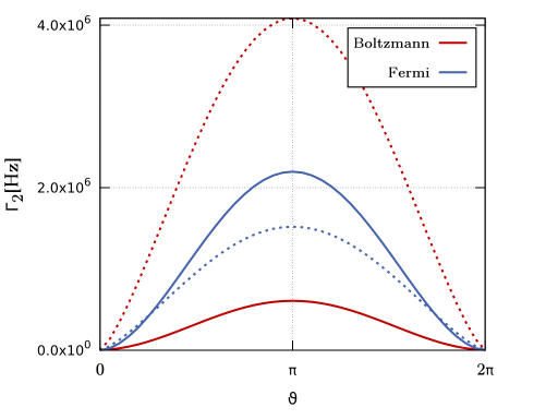
Figure 2: Selfconsistent rate $\Gamma_{2^{*}}$ versus $\vartheta$ for an effective Boltzmann (blue) and Fermi (red) distribution function. Solid lines are numerical iterations of the selfconsistent equation (III.2) while dashed lines are obtained from the analytical approximation (42). The approximation overestimates the rate strongly for the Boltzmann case. This can readily be explained with due to the small rates $\Gamma\ll 1$MHz. The Lorentzian weighting function in the selfconsistent equation has a very narrow peak which measures the spectral density only at small frequencies while for the $x_{qp}$ approximation all quasiparticles are taken into account within the quasiparticle density. For the narrow Fermi distribution the approximation is better because their are no quasiparticles present at higher energies

The effect of tunneling quasiparticles on qubit dephasing is determined by two main factors: the form of the quasiparticle distribution function and the qubit matrix element interference factor $\cos\vartheta=(\text{Re}(\beta_{z}^{2})-\text{Im}(\beta_{z}^{2}))/|\beta_{z}|^{2}$. For purely real matrix element $\beta_{z}$ this factor equals one and the spectral density tends to zero as $\omega$ approaches zero. In this special case dephasing due to quasiparticles remains small and can be neglected compared to the $T_{1}$ time. Any other case offers the possibility of large pure dephasing due to the log divergence. In figure 2 we show the selfconsistent dephasing rate for the same qubit parameters and quasiparticle distribution functions as in the previous section. The rate increases with interference $\vartheta$ until it reaches a maximum at $\vartheta=\pi$. Nonetheless for the Boltzmann distribution it remains small compared to $\Gamma_{1}$: $\Gamma_{2^{*}}\sim\mathcal{O}(0.1\text{MHz})$ while $\Gamma_{1}\sim 1.4\text{MHz}$ for the parameters used for the dephasing calculations. On the other hand for the narrow distribution it becomes comparable and must be taken into account for decoherence if $\cos\vartheta\neq 1$.

V Conclusion

In this work we analyzed qubit dephasing due to quasiparticle tunneling. We applied two different techniques to the problem at hand. First we assumed Markovian behavior and used a self-consistent Born approximation to find a selfconsistent equation for the pure dephasing rate. The rate defined in equation (42) is identical to the one defined in equation (28) fromCatelani et al. (2012) and we want to recommend this work for a more detailed analysis of the selfconsistent rate. But as is known from 1/f noise pure dephasing for a noise with irregular spectral density at zero frequency does usually not follow a simple exponential law with linear exponent. We therefore extended our calculations for non-Markovian behavior and found a dephasing function similar to the Ramsey dephasing functions known for bosonic noiseIthier et al. (2005). We showed that pure dephasing obeys exponential decay with exponent $\sim t^{\alpha}$ with exponent $\alpha\sim-1/2\dots 3/2$ for short times while for longer time scales the dephasing function becomes more and more linear and similar to the selfconsistently obtained rate. The pure dephasing remains small and does not limit qubit coherence for the transmon and similar qubits.

References

- Devoret and Schoelkopf (2013) M. H. Devoret and R. J. Schoelkopf, Science 339, 1169–1174 (2013).
- Bouchiat et al. (1998) V. Bouchiat, D. Vion, P. Joyez, D. Esteve, and M. Devoret, Physica Scripta 1998, 165 (1998).
- Mooij (1999) J. E. Mooij, Science 285, 1036–1039 (1999).
- Martinis et al. (2002) J. Martinis, S. Nam, J. Aumentado, and C. Urbina, Physical Review Letters 89 (2002), 10.1103/physrevlett.89.117901.
- Koch et al. (2007) J. Koch, T. Yu, J. Gambetta, A. Houck, D. Schuster, J. Majer, A. Blais, M. Devoret, S. Girvin, and R. Schoelkopf, Phys. Rev. A 76 (2007), 10.1103/physreva.76.042319, arXiv:cond-mat/0703002v2 [cond-mat.mes-hall] .
- Paik et al. (2011) H. Paik, D. Schuster, L. Bishop, G. Kirchmair, G. Catelani, A. Sears, B. Johnson, M. Reagor, L. Frunzio, L. Glazman, S. Girvin, M. Devoret, and R. Schoelkopf, Physical Review Letters 107, 240501 (2011), arXiv:1105.4652v4 [quant-ph] .
- Rigetti et al. (2012) C. Rigetti, J. M. Gambetta, S. Poletto, B. L. T. Plourde, J. M. Chow, A. D. Córcoles, J. A. Smolin, S. T. Merkel, J. R. Rozen, G. A. Keefe, and et al., Phys. Rev. B 86 (2012), 10.1103/physrevb.86.100506, arXiv:1202.5533v1 [quant-ph] .
- Sears et al. (2012) A. Sears, A. Petrenko, G. Catelani, L. Sun, H. Paik, G. Kirchmair, L. Frunzio, L. Glazman, S. Girvin, and R. Schoelkopf, Physical Review B 86 (2012), arXiv:1206.1265v1 [quant-ph] .
- Barends et al. (2013) R. Barends, J. Kelly, A. Megrant, D. Sank, E. Jeffrey, Y. Chen, Y. Yin, B. Chiaro, J. Mutus, C. Neill, and et al., Physical Review Letters 111 (2013), 10.1103/physrevlett.111.080502, arXiv:1304.2322v1 [quant-ph] .
- Martinis et al. (2009) J. Martinis, M. Ansmann, and J. Aumentado, Physical Review Letters 103 (2009), 10.1103/physrevlett.103.097002.
- Barends et al. (2011) R. Barends, J. Wenner, M. Lenander, Y. Chen, R. C. Bialczak, J. Kelly, E. Lucero, P. O’Malley, M. Mariantoni, D. Sank, and et al., Appl. Phys. Lett. 99, 113507 (2011), arXiv:1105.4642v1 [cond-mat.mes-hall] .
- Lenander et al. (2011) M. Lenander, H. Wang, R. C. Bialczak, E. Lucero, M. Mariantoni, M. Neeley, A. D. O’Connell, D. Sank, M. Weides, J. Wenner, and et al., Phys. Rev. B 84 (2011), 10.1103/physrevb.84.024501, arXiv:1101.0862v1 [cond-mat.supr-con] .
- Shaw et al. (2008) M. Shaw, R. Lutchyn, P. Delsing, and P. Echternach, Phys. Rev. B 78 (2008), 10.1103/physrevb.78.024503, arXiv:0803.3102v3 [cond-mat.mes-hall] .
- Lutchyn et al. (2005) R. Lutchyn, L. Glazman, and A. Larkin, Phys. Rev. B 72 (2005), 10.1103/physrevb.72.014517, arXiv:cond-mat/0503028v2 [cond-mat.mes-hall] .
- Leppäkangas and Marthaler (2012) J. Leppäkangas and M. Marthaler, Phys. Rev. B 85 (2012), 10.1103/physrevb.85.144503, arXiv:1109.2941v1 [cond-mat.mes-hall] .
- Catelani et al. (2011a) G. Catelani, R. J. Schoelkopf, M. H. Devoret, and L. I. Glazman, Phys. Rev. B 84 (2011a), 10.1103/physrevb.84.064517, arXiv:1106.0829v1 [cond-mat.mes-hall] .
- Ithier et al. (2005) G. Ithier, E. Collin, P. Joyez, P. Meeson, D. Vion, D. Esteve, F. Chiarello, A. Shnirman, Y. Makhlin, J. Schriefl, and et al., Phys. Rev. B 72 (2005), 10.1103/physrevb.72.134519.
- Ristè et al. (2013) D. Ristè, C. C. Bultink, M. J. Tiggelman, R. N. Schouten, K. W. Lehnert, and L. DiCarlo, Nature Communications 4, 1913 (2013), arXiv:1212.5459v1 [cond-mat.mes-hall] .
- Catelani (2014) G. Catelani, Phys. Rev. B 89 (2014), 10.1103/physrevb.89.094522, arXiv:1401.5575v1 [cond-mat.mes-hall] .
- Catelani et al. (2012) G. Catelani, S. E. Nigg, S. M. Girvin, R. J. Schoelkopf, and L. I. Glazman, Phys. Rev. B 86 (2012), 10.1103/physrevb.86.184514, arXiv:1207.7084v1 [cond-mat.mes-hall] .
- Pop et al. (2014) I. M. Pop, K. Geerlings, G. Catelani, R. J. Schoelkopf, L. I. Glazman, and M. H. Devoret, Nature 508, 369–372 (2014).
- Bylander et al. (2011a) J. Bylander, S. Gustavsson, F. Yan, F. Yoshihara, K. Harrabi, G. Fitch, D. G. Cory, Y. Nakamura, J.-S. Tsai, and W. D. Oliver, Nat Phys 7, 565–570 (2011a).
- Knill and Laflamme (1997) E. Knill and R. Laflamme, Phys. Rev. A 55, 900–911 (1997).
- Makhlin et al. (2001) Y. Makhlin, G. Schön, and A. Shnirman, Rev. Mod. Phys. 73, 357–400 (2001), arXiv:cond-mat/0011269v1 [cond-mat.mes-hall] .
- Owen and Scalapino (1972) C. Owen and D. Scalapino, Physical Review Letters 28, 1559–1561 (1972).
- Palacios-Laloy et al. (2009) A. Palacios-Laloy, F. Mallet, F. Nguyen, F. Ong, P. Bertet, D. Vion, and D. Esteve, Phys. Scr. T137, 014015 (2009).
- Shor (1995) P. W. Shor, Phys. Rev. A 52, R2493–R2496 (1995).
- Sun et al. (2012) L. Sun, L. DiCarlo, M. D. Reed, G. Catelani, L. S. Bishop, D. I. Schuster, B. R. Johnson, G. A. Yang, L. Frunzio, L. Glazman, and et al., Physical Review Letters 108 (2012), 10.1103/physrevlett.108.230509, arXiv:1112.2621v1 [cond-mat.mes-hall] .
- Catelani et al. (2011b) G. Catelani, J. Koch, L. Frunzio, R. J. Schoelkopf, M. H. Devoret, and L. I. Glazman, Physical Review Letters 106 (2011b), 10.1103/physrevlett.106.077002, arXiv:1101.1341v2 [cond-mat.mes-hall] .
- Bylander et al. (2011b) J. Bylander, S. Gustavsson, F. Yan, F. Yoshihara, K. Harrabi, G. Fitch, D. G. Cory, Y. Nakamura, J.-S. Tsai, and W. D. Oliver, Nat Phys 7, 565–570 (2011b).
- Makhlin et al. (2004) Y. Makhlin, G. Schön, and A. Shnirman, Chemical Physics 296, 315–324 (2004), arXiv:cond-mat/0309049v1 [cond-mat.mes-hall] .
- Wang et al. (2014) C. Wang, Y. Gao, I. Pop, U. Vool, C. Axline, T. Brecht, R. Heeres, L. Frunzio, M. Devoret, G. Catelani, L. Glazman, and R. Schoelkopf, ArXiv e-prints (2014), arXiv:1406.7300v1 [quant-ph] .
- (33) .
- Barends et al. (2014) R. Barends, J. Kelly, A. Megrant, A. Veitia, D. Sank, E. Jeffrey, T. C. White, J. Mutus, A. G. Fowler, B. Campbell, and et al., Nature 508, 500–503 (2014), arXiv:1402.4848v1 [quant-ph] .