Detection of a quantum particle on a lattice under repeated projective measurements

Abstract

We consider a quantum particle, moving on a lattice with a tight-binding Hamiltonian, which is subjected to measurements to detect it’s arrival at a particular chosen set of sites. The projective measurements are made at regular time intervals $\tau$, and we consider the evolution of the wave function till the time a detection occurs. We study the probabilities of its first detection at some time and conversely the probability of it not being detected (i.e., surviving) up to that time. We propose a general perturbative approach for understanding the dynamics which maps the evolution operator, consisting of unitary transformations followed by projections, to one described by a non-Hermitian Hamiltonian. For some examples, of a particle moving on one and two-dimensional lattices with one or more detection sites, we use this approach to find exact expressions for the survival probability and find excellent agreement with direct numerical results. A mean field model with hopping between all pairs of sites and detection at one site is solved exactly. For the one- and two-dimensional systems, the survival probability is shown to have a power-law decay with time, where the power depends on the initial position of the particle. Finally, we show an interesting and non-trivial connection between the dynamics of the particle in our model and the evolution of a particle under a non-Hermitian Hamiltonian with a large absorbing potential at some sites.

I Introduction

The measurement of the arrival time of a quantum mechanical particle in a given detection region is a longstanding and fundamental problem in quantum mechanics allcock69 ; kijowski74 ; kumar85 ; grott96 ; aharonov98 ; savvidou06 ; mugap00 ; damborenea02 ; galapon04 ; galapon05 ; muga08 ; yearsley ; savvidou12 ; vona13 ; muga00 ; vega1 ; vega2 . In spite of much effort, the construction of a time operator has been found to be controversial mielnik . One possible approach that one could take to find the time of arrival is the following. Suppose that a particle is released from a given region at time $t=0$ and is allowed to evolve unitarily with some Hamiltonian. In some specified detection region we make repeated instantaneous, projective measurements, at regular time intervals $\tau$, to see if the particle has arrived there, and we stop once a detection is made. If the detection occurs at the $n^{\rm th}$ measurement, we could say that the particle’s time of arrival into the detection region, is at time $t=n\tau$ (or more precisely between times $t-\tau$ and $t$). Repeated measurements of this kind are known to have a somewhat surprising feature when one considers the limit where the time interval between measurements $\tau$ is taken to zero. One finds that the probability of detecting the particle goes to zero; this is called the quantum Zeno effect misra77 ; shimizub05 ; facchi08 ; wineland90 ; kofman ; kwiat ; cirac ; itano09 ; signoles .

An interesting case to consider is one where the time $\tau$ between measurements is assumed to be small compared to the typical spreading time of a wave packet (in the models that we will study, the spreading time is of the order of $1/\gamma$, where $\gamma$ is the hopping amplitude between nearest neighbors), but is kept finite and we do not take the limit $\tau\to 0$. The problem of the effect of repeated measurements, made at finite time intervals, on the evolution of a quantum system has been studied in various contexts both theoretically and experimentally hegerfeldt96 ; erez08 ; jahnke ; christian12 ; halliwell10 ; ingold11 . Because of the probabilistic nature of the quantum detection process, we expect the time of detection to be a stochastic variable. The probability distribution of this time of first detection of the particle in some given region, and the complementary probability of not being detected (i.e., survival) at all up to some time, are then interesting quantities to study. The time evolution of the wave function of a surviving particle is also of interest.

In an earlier paper dhar13 , we addressed this problem taking the example of a particle moving on a one-dimensional lattice with a tight-binding Hamiltonian, with detections made at a single site. This paper extends our earlier work in several directions. We consider here the motion of a single particle on an arbitrary lattice, with the dynamics still controlled by a tight-binding Hamiltonian. Also, we allow our projective measurements to be made on more than one site in a region. Through a general perturbative treatment, valid when the time interval between measurements is small compared to the wave spreading time scale, we show that the long time dynamics of the particle can be effectively described by a non-Hermitian Hamiltonian. The non-Hermitian Hamiltonian is defined on the subspace consisting of non-measurement sites and contains a small imaginary potential on all the sites that are connected directly by hopping to the measurement sites. Using this result, we are able to solve for the time evolution of initially localized wave functions and from this, analytically compute the survival probability for several examples of particles in one- and two-dimensional lattices. Our analytic results are compared with direct numerical results and we find excellent agreement. We find that the survival probability decays as a power of the time, where the power depends on the initial position of the particle. Finally, we demonstrate another mapping that can be made between the effective non-Hermitian Hamiltonian with a small imaginary potential that appears in our model, and a different non-Hermitian Hamiltonian which has a large imaginary potential on the measurement sites. This second non-Hermitian Hamiltonian is similar to what has been proposed in the context of the study of the time of arrival of a free quantum particle (moving in continuous space) into a given region (the half line), using the approach of repeated measurements muga08 ; halliwell10 . This also relates our study to a recent work of Krapivsky et al  mallick13 who look at the survival probability of a particle moving on a one-dimensional lattice with imaginary potentials at one or more sites.

The plan of the paper is as follows. In Sec. II, we describe our precise model and the repeated measurement protocol. We show that the measurement dynamics is described by an effective non-unitary evolution operator which evolves the wave function between successive measurements. We explain how an expression for the survival probability $P_{n}$ after the $n^{\rm th}$ measurement can be obtained from the wave function. In Sec. III we describe the perturbation theory by which we are able to describe the non-unitary dynamics by an effective non-Hermitian Hamiltonian. In Sec. IV we consider several examples of a single quantum particle moving on one- and two-dimensional lattices and described by tight-binding Hamiltonians with nearest neighbor hopping terms, which is subjected to regular measurements made on one or more sites at regular intervals of time $\tau$. We derive perturbative results for the survival probability and the effective wave function of the particle after a time given by an integer multiple of $\tau$. Analytical and numerical results are presented. We also present (Sec. V) an exact solution for a mean field type of model where the particle can hop from any site to all the other sites. Sec. VI describes the mapping between the non-Hermitian Hamiltonian problem with a large imaginary potential at the measurement sites and our problem with small measurement time intervals. We conclude with a discussion in Sec. VII.

II Model and general framework

Our model consists of a particle moving on a discrete lattice of $N$ sites and its dynamics is described by a tight-binding type Hamiltonian of the form

$$H=\sum_{\begin{subarray}{c}r,s=1\end{subarray}}^{N}H_{r,s}~{}|r\rangle\langle s|~{},$$ (1)

where $H$ is taken to be a real symmetric matrix whose non-vanishing elements have strength $\gamma$ (in units of $\hbar$). The free time evolution of $|\psi\rangle$ is given by

$$|\psi(t)\rangle=U_{t}|\psi(0)\rangle,~{}~{}{\rm where}~{}~{}U_{t}=e^{-iHt}~{}.$$ (2)

Let us define the projection operator ${A}=\sum_{r\in D}|r\rangle\langle r|$ corresponding to a measurement to detect the particle in the domain $D$ containing a fixed number $N_{D}$ of sites, and the complementary operator $B=1-A$ corresponding to the projection to the space of $N_{S}$ sites belonging to the “system”. According to the measurement postulate of quantum mechanics, the probability of detecting the particle on performing a measurement on the state $|\psi\rangle$ is $p=\sum_{r\in D}|\langle r|\psi\rangle|^{2}=\langle\psi|A|\psi\rangle$. The probability of non-detection or the survival probability is then $P=\langle\psi|B|\psi\rangle=1-p$. The measurement postulate also tells us about the state of the system immediately after the measurement. They in fact alter the Hamiltonian time evolution of the system. If the measurement detects the particle (with probability $p$) then the state after measurement is $A|\psi\rangle$, while if a measurement does not detect the particle (with probability $P$), then the state immediately after measurement is $|\psi^{+}\rangle=B|\psi\rangle$, with appropriate normalizations. Thus we see that after the measurement the system is effectively described by a density matrix $\rho^{\prime}=A|\psi\rangle\langle\psi|A+B|\psi\rangle\langle\psi|B$. However in our scheme we stop the experiment whenever a particle is detected. Hence only those states that are projected onto the system subspace are further evolved, and we do not need to consider density matrices. After the first measurement we again unitarily evolve the state $|\psi^{+}\rangle=B|\psi\rangle$ until the next measurement.

We consider a sequence of measurements $n=1,2\ldots$ at intervals of time $\tau$ which continue until a particle is detected. Thus the time evolution is given by a sequence of unitary evolutions followed by projections, onto the subspace corresponding to $B$, till the particle is detected. Let $|\psi^{-}_{n}\rangle$ and $|\psi^{+}_{n}\rangle$ be the (un-normalized) wave functions of the system, immediately before and after the $n^{\rm th}$ measurement respectively. We note that $|\psi^{-}_{n}\rangle=U_{\tau}|\psi^{+}_{n-1}\rangle$ and $|\psi^{+}_{n}\rangle=B|\psi^{-}_{n}\rangle$. Hence, defining ${\widetilde{U}}=BU_{\tau}$, it follows that

$$|\psi^{-}_{n}\rangle=U_{\tau}{\widetilde{U}}^{n-1}|\psi(0)\rangle~{}~{}~{}{\rm and}~{}~{}~{}|\psi^{+}_{n}\rangle={\widetilde{U}}^{n}|\psi(0)\rangle~{}.$$ (3)

Let $P_{n}$ be the probability of survival after $n$ measurements. Then clearly

$$P_{1}=\langle\psi^{-}_{1}|B|\psi^{-}_{1}\rangle=\langle\psi(0)|{\widetilde{U}}^{\dagger}{\widetilde{U}}|\psi(0)\rangle=\langle\psi^{+}_{1}|\psi^{+}_{1}\rangle~{}.$$

Note that $P_{1}$ is thus the normalizing factor for $|\psi^{+}_{1}\rangle$ and also for $|\psi^{-}_{2}\rangle$. The survival probability after the second measurement is obtained as the product of non-detection at $n=1$ times the probability of non-detection at $n=2$, and is given by

$$P_{2}=P_{1}\times\frac{\langle\psi^{-}_{2}|}{\sqrt{P_{1}}}B\frac{|\psi^{-}_{2}\rangle}{\sqrt{P_{1}}}=\langle\psi(0)|{\widetilde{U}}^{\dagger 2}{\widetilde{U}}^{2}|\psi(0)\rangle=\langle\psi^{+}_{2}|\psi^{+}_{2}\rangle~{}.$$

Proceeding iteratively in this way, we get

$$P_{n}=\langle\psi(0)|{\widetilde{U}}^{\dagger n}{\widetilde{U}}^{n}|\psi(0)\rangle=\langle\psi^{+}_{n}|\psi^{+}_{n}\rangle~{}.$$ (4)

If we imagine an ensemble of identically prepared states on which we perform repeated measurements, then $P_{n}=\langle\psi^{+}_{n}|\psi^{+}_{n}\rangle$ gives the fraction of systems for which there has been no detection and that are still evolving. The probability of first detection in the $n^{\rm th}$ measurement is given by

$$p_{n} =P_{n-1}\times\frac{\langle\psi^{-}_{n}|}{\sqrt{P_{n-1}}}A\frac{|\psi^{-}_{n}\rangle}{\sqrt{P_{n-1}}}=\langle\psi^{-}_{n}|A|\psi^{-}_{n}\rangle~{}$$ (5)

$$=\langle\psi^{-}_{n}|\psi^{-}_{n}\rangle-\langle\psi^{-}_{n}|B|\psi^{-}_{n}\rangle=P_{n-1}-P_{n}~{},$$ (6)

as expected.

Our main aim in the rest of the paper is to study the behavior of the survival probability for different cases. From the discussion above it is clear that the central problem is to understand the properties of the effective evolution operator ${\widetilde{U}}$ which, for initial states located inside the “system”, is equivalently given by

$${\widetilde{U}}\equiv Be^{-iH\tau}B~{}.$$ (7)

An explicit diagonalization of this non-Hermitian evolution operator is difficult in general. In the next section we provide a perturbative approach, valid for small $\tau<<1/\gamma$. As we will see from our numerical results, this gives a quite accurate description.

III Perturbation theory and connection to an effective non-Hermitian Hamiltonian

Let us use the following notation: we divide our full set of sites into those belonging to the “system” (labeled by roman indices $l,m$) and those belonging to the domain $D$ consisting of sites where measurements are made (denoted by greek indices $\alpha,\beta$). With this notation we have $A=\sum_{\alpha}|\alpha\rangle\langle\alpha|$ and $B=\sum_{l}|l\rangle\langle l|$, while the Hamiltonian in Eq. (1) can be rewritten in the following form

$$H =H_{S}+H_{M}+V~{},$$ (8)

$${\rm where}~{}~{}H_{S} =\sum_{l,m}H_{l,m}|l\rangle\langle m|,~{}~{}~{}H_{M}=\sum_{\alpha,\beta}H_{\alpha,\beta}|\alpha\rangle\langle\beta|,~{}~{}~{}$$

$${\rm and}~{}~{}V =\sum_{l,\alpha}V_{l,\alpha}|l\rangle\langle\alpha|+V_{\alpha,l}|\alpha\rangle\langle l|,$$

describe the system, measurement sites and coupling parts respectively of the full Hamiltonian.

Expanding the effective evolution operator ${\widetilde{U}}=Be^{-iHt}B$ to second order in $\tau$ gives in the system subspace,

$${\widetilde{U}} =B~{}\left[~{}I-iH\tau-\frac{\tau^{2}}{2}H^{2}+\ldots~{}\right]~{}B$$

$$=I-iH_{S}\tau-\frac{\tau^{2}}{2}H_{S}^{2}$$

$$-\frac{\tau^{2}}{2}\sum_{l,m}\sum_{\alpha}V_{l,\alpha}V_{\alpha,m}|l\rangle\langle m|+\ldots$$

$$=e^{-iH_{eff}\tau}+{\mathcal{O}}(\tau^{3}),$$

$${\rm where}~{}~{}H_{eff} =H_{S}+V_{eff},$$ (9)

$${\rm and}~{}~{}V_{eff} =-\frac{i\tau}{2}\sum_{l,m}\sum_{\alpha}V_{l,\alpha}V_{\alpha,m}|l\rangle\langle m|~{}.$$

($I$ denotes the $N_{S}\times N_{S}$ unit matrix). Thus we see that our system is effectively described by a non-Hermitian Hamiltonian $H_{eff}$ and the problem now reduces to diagonalizing this Hamiltonian. Note in particular that the strength of the non-Hermitian potential is small and proportional to the measurement interval $\tau$. In the following section we will give explicit examples on regular lattices in one and two dimensions where this reduced problem can be tackled analytically, and comparisons can be made with direct numerical solutions of the original problem.

IV Comparisons between perturbation theory and direct numerical results

IV.1 Particle in a one-dimensional box

We consider the motion of a quantum particle in a one-dimensional lattice with only nearest neighbor hoppings and open boundary conditions. The corresponding full Hamiltonian is

$$H=-~{}\gamma~{}\sum_{l=1}^{N-1}\left(~{}|l+1\rangle\langle l|+|l\rangle\langle l+1|~{}\right)~{}.$$

Without loss of generality we set $\gamma=1$. We consider three different cases corresponding to different choices of the measurement points: (i) $\alpha=N$, (ii) $\alpha=N-N_{D}+1,N-N_{D}+2,\ldots,N$ and (iii) $\alpha=1,N$.

Case (i): Measurement at single point at one end of the box.
This case was presented elsewhere dhar13 but we present it here again as an illustrative example of our present general framework. The projection operators now are ${A}=|N\rangle\langle N|$ and $B=\sum_{l=1}^{N-1}|l\rangle\langle l|$. From the general discussion in Sec. III it is clear that the effective Hamiltonian for the $N-1$ sites system is given by

$$H_{eff} =H_{S}+V_{eff},$$

$${\rm where}~{}~{}H_{S}= -\sum_{l=1}^{N-2}\left(~{}|l+1\rangle\langle l|+|l\rangle\langle l+1|~{}\right)~{}~{}{\rm and}$$

$$V_{eff}=-\frac{i\tau}{2}|N-1\rangle\langle N-1|~{}.$$ (10)

We now obtain the eigenvalues and eigenvectors of this effective Hamiltonian using first order perturbation theory. The eigenvalues of $H_{S}$ (with $N-1$ sites) are given by

$$\epsilon_{s}=-2\cos\left(\frac{s\pi}{N}\right),$$ (11)

while the eigenvectors $\langle l|\phi_{s}\rangle=\phi_{s}(l)$ are given by

$$\phi_{s}(l)=\sqrt{\frac{2}{N}}\sin\left(\frac{sl\pi}{N}\right)$$ (12)

for $s=1,2,\ldots,N-1$. Treating $V_{eff}$ as a perturbation, we find the following modified spectrum for $H_{eff}$,

$$\mu_{s} =\epsilon_{s}+\langle\phi_{s}|V_{eff}|\phi_{s}\rangle=\epsilon_{s}-\frac{i}{2}\alpha_{s},$$ (13)

$${\rm with}~{}~{}\alpha_{s} =\frac{2\tau}{N}\sin^{2}\left(\frac{s\pi}{N}\right)~{}.$$ (14)

This means that an eigenstate of $H_{S}$ will decay with time and, after $n$ measurements made at times $t=n\tau$, the state of the system is given by

$$|\phi_{s}(t)\rangle=e^{-iH_{eff}t}|\phi_{s}\rangle=e^{-\alpha_{s}t/2}e^{-i\epsilon_{s}t}|\phi_{s}\rangle.$$

Hence the survival probability $P_{s}(t)$ is given by the exponential decay

$$P_{s}(t)=\langle\phi_{s}(t)|\phi_{s}(t)\rangle=e^{-\alpha_{s}t}~{},$$

and the first detection probability by $p(t)=-dP/dt=\alpha_{s}e^{-\alpha_{s}t}$. Since the decay rate $\alpha_{s}$ depends on $\tau$, it vanishes in the limit $\tau\to 0$, and one obtains the quantum Zeno effect.

When the initial state is a position eigenstate , it has been shown dhar13 that the time evolution is given by

$$|\psi(t)\rangle=e^{-iH_{eff}t}|\ell\rangle=\sum_{s}\phi_{s}(\ell)e^{-\alpha_{s}t/2}e^{-i\epsilon_{s}t}|\phi_{s}\rangle~{},$$ (15)

and thus the survival probability becomes

$$P_{\ell}(t) =\langle\psi(t)|\psi(t)\rangle=\sum_{s=1}^{N}\frac{2}{N}\sin^{2}(\frac{s\pi\ell}{N})e^{-\frac{2\tau t}{N}\sin^{2}(\frac{s\pi}{N})}~{}.$$ (16)

For large $N$ and in the time window where $t\tau/N$ is large but $t\tau/N^{3}$ is small, Eq.  (16) becomes

$$P_{\ell}(t)=\frac{1}{\sqrt{8\pi x}}\left[1-e^{-\ell^{2}/2x}\right],~{}~{}~{}{\rm where}~{}~{}~{}x=\frac{t\tau}{N}.$$ (17)

If the particle was initially close to the left boundary ($\ell\sim O(1)$), then the survival probability decays as $1/t^{1/2}$ for small $t$ and as $1/t^{3/2}$ for large $t$. On the other hand, if the particle was initially well within the bulk ($\ell\sim O(N)$), then one observes only the former behavior of $1/t^{1/2}$. At times $t\sim N^{3}$ there is an exponential decay with time. We show in Fig. 1 the decay of the survival probability with time, as computed numerically from the exact expression in Eq.  (4) and from the analytical perturbative expression in Eq. (16). It is clear that there is very good agreement between the direct results and those obtained from perturbation theory. The form of the wave functions at different times is shown in Fig. 2. We see that at large times ($O(N^{3})$) the wave function gets a contribution mainly from the lowest eigenstate and one can understand the exponential decay at these time scales. Another interesting feature is that the behaviors for $\ell$ and $N-\ell$ are the same, $P_{\ell}(t)=P_{N-\ell}(t)$, due to the symmetry $\phi_{s}({\ell})=\phi_{s}({N-\ell})$.

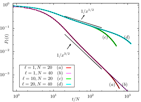
Figure 1: (Color online) Open Boundary Conditions: Decay of the survival probability $P_{\ell}(t)$ for different initial position egenstates. The black dotted lines are the predictions from perturbation theory. The solid black lines are the predicted power law decays for initial points in the bulk and at the boundary. The measurement was done at site $N$, and the measurement time interval was taken to be $\tau=0.1$.

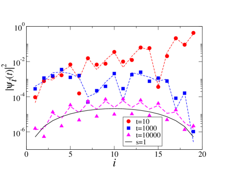
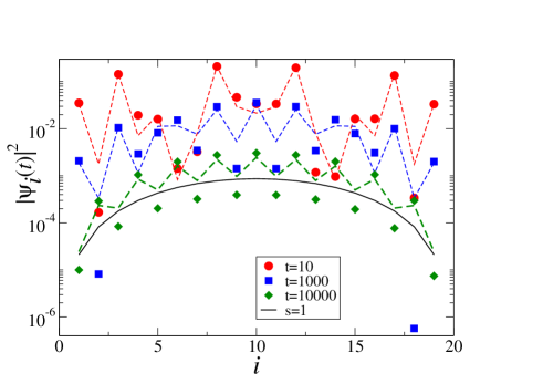
Figure 2: (Color online) Open Boundary Conditions: Plot of the probability density $|\psi_{i}(t)|^{2}$ at different times when the initial state is a position eigenstate with (top)$\ell=1$ and (bottom)$\ell=10$. The dashed lines are the predictions from the perturbation theory [Eq. (15)]. The solid line is the plot for the lowest eigenstate. The other parameters were $N=20$ and $\tau=0.1$.

Case (ii): One-dimensional box with measurements done on several sites at one end.

In this case the measurement projection operator is given by $A=\sum_{\alpha=N-N_{D}+1}^{N}|\alpha\rangle\langle\alpha|$ and the system consists of $N_{S}=N-N_{D}$ points. We notice that, because of the nearest neighbor coupling form of the Hamiltonian, the form of $V_{eff}$ is now given by $V_{eff}=-i(\tau/2)|N-N_{D}><N-N_{D}|$. Hence the analysis of the previous case remains valid with the simple replacement $N-1\to N-N_{D}$. In particular, we recover the same asymptotic behavior for the survival probability. Physically we can understand this result as follows — since $\tau$ is small, the particle can propagate only up to one site during time $\tau$. Thus the systems with $1$ and $N_{D}$ measurement sites at the end are the same (for $N_{D}>1$) as the particle never visits sites beyond the first detector site.

Case (iii): One-dimensional box with measurement done at boundary sites on both ends.

The measurement projection operator now is $A=|1\rangle\langle 1|+|N\rangle\langle N|$ and the number of sites on the system is $N-2$. The effective interaction is then given by $V_{eff}=-(i\tau/2)(|2\rangle\langle 2|+|N-1\rangle\langle N-1|)$. The eigenstates of $H_{S}$ (with $N-2$ sites) are now given by

$$\phi^{\prime}_{s}(l)=\sqrt{\frac{2}{N-1}}\sin\left(\frac{s\pi(l-1)}{N-1}\right),$$

with $s=1,2,\ldots,N-2$ and $l=2,3,\ldots,N-1$, and the eigenvalues of $H_{eff}$ are given by $\mu_{s}=\epsilon^{\prime}_{s}-(i/2)\alpha^{\prime}_{s}$, with $\epsilon^{\prime}_{s}=-2\cos[s\pi/(N-1)]$ and $\alpha^{\prime}_{s}=\tau[\phi^{\prime 2}_{s}(2)+\phi^{\prime 2}_{s}(N-1)]=[4\tau/(N-1)]~{}\sin^{2}[s\pi/(N-1)]$. Thus, for large $N$, we get a decay constant for the eigenstates which has twice the value of that in case (i), corresponding to the fact that there is absorption at two boundary points. Clearly the asymptotic results given for case (i) for survival probability of initial position eigenstates continue to hold.

IV.2 One-dimensional lattice with periodic boundary conditions

We now consider a ring geometry with a Hamiltonian given by

$${H}=-\sum_{l=1}^{N}\left(~{}|l+1\rangle\langle l|+|l\rangle\langle l+1|~{}\right)~{}$$ (18)

with $|N+1\rangle\equiv|1\rangle$, and we assume that $N$ is even. This case was also presented in Ref. dhar13 and we discuss it now within the present framework. Taking $A=|N\rangle\langle N|$ we get $H_{S}=\sum_{l=1}^{N-2}~{}(|l+1\rangle\langle l|+|l\rangle\langle l+1|)$ (the same as that for Case (i)), and $V_{eff}=(-i\tau/2)(|N-1\rangle\langle N-1|+|1\rangle\langle 1|+|N-1\rangle\langle 1|+|1\rangle\langle N-1|)$.

This case is somewhat special because it turns out that half of the energy eigenstates of $H$ are unaffected by the measurement process. To see this we notice that there are $(N-2)/2$ eigenvalues of $H$, given by $e_{s}=-2\cos(2s\pi/N)$, for $s=1,2,\ldots,N/2-1$, which are two-fold degenerate with eigenvectors

$$\psi_{s}(l)=\sqrt{\frac{2}{N}}\sin\frac{2sl\pi}{N}~{}~{}~{}~{}{\rm and}~{}~{}~{}~{}\psi_{s+N/2-1}(l)=\sqrt{\frac{2}{N}}\cos\frac{2sl\pi}{N}.$$ (19)

The remaining two eigenvalues $-2$ and $2$ correspond respectively to eigenvectors

$$\psi_{N-1}(l)=(-1)^{l}/\sqrt{N}~{}~{}~{}~{}{\rm and}~{}~{}~{}~{}\psi_{N}(l)=1/\sqrt{N}.$$

We now observe that $\psi_{s}(l)$, for $s=1,\ldots,N/2-1$, are also exact eigenstates of the Hamiltonian for an open chain with $N-1$ sites $l=1,\ldots,N-1$. Let us denote these eigenstates of $H_{S}$ by $\phi_{2s}(l)$ and the corresponding eigenvalues by $\epsilon_{2s}=e_{s}$. Since $\phi_{2s}(l)$ vanish at the detector site $l=N$, they are not affected by the measurements and are exact eigenfunctions of $\widetilde{U}$. The rest of the eigenstates of $H_{S}$, given by $\phi_{2s+1}(l)=\sqrt{{2}/{N}}\sin[(2s+1)l\pi/{N}]$ with eigenvalues $\epsilon_{2s+1}=2\cos[(2s+1)\pi/N]$, for $s=0,1,\ldots,N/2-1$, decay with a rate which we can again compute from perturbation theory. We find

$$\alpha_{2s+1}=-\frac{2}{i}\langle\phi_{2s+1}|V_{eff}|\phi_{2s+1}\rangle=4\tau\phi^{2}_{2s+1}(1).$$ (20)

If the particle is initially at site $\ell$, its time evolution is given by

$$|\psi(t)\rangle =\sum_{s=1}^{N/2-1}\phi_{2s}(\ell)e^{-i\epsilon_{2s}t}|\phi_{2s}\rangle~{}+$$

$$\sum_{s=0}^{N/2-1}\phi_{2s+1}(\ell)P^{1/2}_{2s+1}(t)e^{-i\epsilon_{2s+1}t}|\phi_{2s+1}\rangle,$$ (21)

so that,

$$P_{\ell}(t)-P_{\ell}(\infty)=\sum_{s=0}^{N/2-1}\phi_{2s+1}^{2}(\ell)P_{2s+1}(t).$$ (22)

For large $N$ and large $t\tau/N(=x)$, Eq. (22) becomes

$$P_{\ell}(t)-P_{\ell}({\infty}) =\frac{1}{2\pi}\int_{-\infty}^{\infty}dq\sin^{2}(q\ell)e^{-8xq^{2}}$$

$$=\frac{1}{8\sqrt{2\pi x}}\left[1-e^{-\ell^{2}/8x}\right],$$ (23)

with $P_{l}(\infty)=\sum_{s=1}^{N/2-1}\phi_{2s}^{2}(\ell)$ which is equal to $1/2$ for $\ell\neq N/2$ and zero for $\ell=N/2$. Thus, $P_{\ell}(t)-P_{\ell}(\infty)$ decays as $1/t^{1/2}$ when the initial position $\ell$ is in the bulk, and as $1/t^{3/2}$ when $\ell$ is near the boundary. Furthermore, when $\ell=N$ the decay is of order $1/t^{1/2}$ and $P_{N}(\infty)=0$.

In Fig. 3 we show the comparison between the analytical predictions for the survival probability from Eq. (22) and the numerical results obtained directly from Eq. (4); they show reasonably good agreement. The form of the wave functions at different times is shown in Fig. 4. We see that as in the case of open boundary conditions, at large times (${\cal O}(N^{3})$) the wave function gets a contribution mainly from the surviving eigenstates (for $\ell=1$) or from the lowest eigenstate (for the special case $\ell=N/2$).

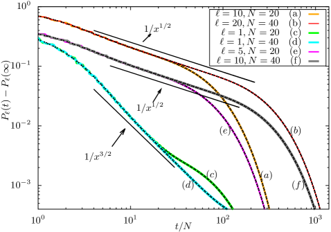
Figure 3: (Color online) Periodic Boundary Conditions: Decay of the survival probability $P_{\ell}(t)$ for different initial position eigenstates and different system sizes. The upper-most two plots are for $\ell=N/2$ in which case the survival probability at infinite times $P_{\ell}(\infty)$ vanishes, while in all the other cases $P_{\ell}(\infty)=0.5$. The black dotted lines are the predictions from perturbation theory. The solid black lines are the predicted power law decays for bulk and boundary points. The measurement was done at site $N$, and the measurement time interval was taken to be $\tau=0.1$.

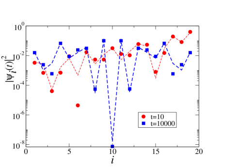
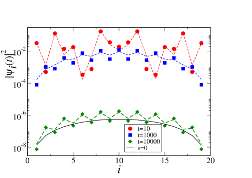
Figure 4: (Color online) Periodic Boundary Conditions: Plot of the probability density $|\psi_{i}(t)|^{2}$ at different times when the initial state is a position eigenstate with (top)$\ell=1$ and (bottom)$\ell=10$. The dashed lines are the predictions from the perturbation theory [Eq. (21)]. The solid line in the bottom panel is the plot for the lowest eigenstate. The other parameters were $N=20$, $\tau=0.1$.

Figure 5: Different arrangements of detectors (shown by thick lines) for a system on a square lattice. The $(1,1)$ site is at the top left corner, and the $x$, $y$ axes are horizontal (to the right) and vertical (downwards).

IV.3 Particle in a two-dimensional box with multiple detection points

In this case the Hamiltonian is given by

$$H_{2D} =-~{}\gamma\sum_{l_{x}=1}^{N-1}\sum_{l_{y}=1}^{N-1}[~{}|l_{x}+1,l_{y}\rangle\langle l_{x},l_{y}|+|l_{x},l_{y}\rangle\langle l_{x}+1,l_{y}|$$

$$~{}~{}~{}+~{}|l_{x},l_{y}+1\rangle\langle l_{x},l_{y}|+|l_{x},l_{y}\rangle\langle l_{x},l_{y}+1|~{}]~{}.$$ (24)

Again we work with $\gamma=1$. We note that $H_{2D}$ is a sum of two commuting Hamiltonians describing jumps along the $x$ and $y$ axes,

$$H_{2D}=H_{x}+H_{y},$$ (25)

where

$$H_{x}=-\sum_{l_{x},l_{y}=1}^{N-1}\left(|l_{x}+1,l_{y}\rangle\langle l_{x},l_{y}|+|l_{x},l_{y}\rangle\langle l_{x}+1,l_{y}|\right),$$

and similarly for $H_{y}$. Obviously, $H_{x}=H\otimes I$ and $H_{y}=I\otimes H$, where $H$ is the Hamiltonian for an open chain with $N$ sites, and $I$ is an $N\times N$ unit matrix.

Case (i): Measurement sites placed along one boundary.
We consider measurement sites at $(N,l_{y})$ for $l_{y}=1,2,\ldots,N$. Then $B_{2D}=B\otimes I$, where $B=\sum_{\l=1}^{N-1}|l\rangle\langle l|$, and

$${\widetilde{U}}_{2D} =B_{2D}\exp\left(-iH_{2D}t\right)$$

$$=\left[B\exp\left(-iHt\right)\right]\otimes\left[\exp\left(-iHt\right)\right].$$ (26)

Hence the behavior of $({\widetilde{U}}_{2D})^{n}$ is governed by that of $[B\exp\left(-iHt\right)]^{n}$, indicating that the behavior of the survival probability of this system is identical with that of an open chain (with the same size) with one detector kept at the $N$-th site. Moreover, this equivalence (and similar equivalences derived below) is true for all values of $\tau$, not necessarily small.

Case (ii): Measurement sites placed along two opposite boundaries.

We consider measurement sites at $(1,l_{y})$ and $(N,l_{y})$, for $l_{y}=1,2,\ldots,N$. Then $B_{2D}=B^{\prime}\otimes I$, where $B^{\prime}=\sum_{\l=2}^{N-1}|l\rangle\langle l|$, and

$${\widetilde{U}}_{2D}=\left[B^{\prime}\exp\left(-iHt\right)\right]\otimes\left[\exp\left(-iHt\right)\right].$$ (27)

The behavior of $({\widetilde{U}}_{2D})^{n}$ is hence governed by that of $[B^{\prime}\exp\left(-iHt\right)]^{n}$ indicating that the behavior of the survival probability of this system is identical with that of an open chain with one detector kept at each end (which, in turn, is similar to the survival probability of the chain with a detector at the $N$-th site).

Case (iii): Measurement sites placed along two adjacent boundaries.

We consider measurement sites at $(l_{x},N)$, for $l_{x}=1,2,\ldots,N$ and $(N,l_{y})$, for $l_{y}=1,2,\ldots,(N-1)$. Then $B_{2D}=B\otimes B$, and

$${\widetilde{U}}_{2D}=\left[B\exp\left(-iHt\right)\right]\otimes\left[B\exp\left(-iHt\right)\right].$$ (28)

Hence when the initial state is $|\phi_{s}\rangle\otimes|\phi_{s^{\prime}}\rangle$, the survival probability becomes

$$P_{s,s^{\prime}}(t)=e^{-(\alpha_{s}+\alpha_{s^{\prime}})t}.$$

If the particle is initially at $|\ell_{x}\rangle\otimes|\ell_{y}\rangle$, the survival probability is

$$P_{\ell_{x},\ell_{y}}(t) =\sum_{s,s^{\prime}=1}^{N-1}\phi_{s}^{2}(\ell_{x})\phi_{s^{\prime}}^{2}(\ell_{y})P_{s,s^{\prime}}(t)$$ (29)

$$=\frac{1}{\sqrt{8\pi x}}[1-e^{-\ell_{x}^{2}/2x}]~{}\frac{1}{\sqrt{8\pi x}}[1-e^{-\ell_{y}^{2}/2x}],$$

with $x=t\tau/N$. Thus the survival probability becomes a product of the respective survival probabilities in the two directions, each with one detector at the last site.

Case (iv): Measurement sites placed along three boundaries.

We consider measurement sites at $(1,l_{y})$ and $(N,l_{y})$, for $l_{y}=1,2,\ldots,N$ and $(l_{x},N)$, for $l_{x}=2,\ldots,(N-1)$. Then $B_{2D}=B^{\prime}\otimes B$, and

$${\widetilde{U}}_{2D}=\left[B^{\prime}\exp\left(-iHt\right)\right]\otimes\left[B\exp\left(-iHt\right)\right].$$ (30)

When the initial state is $|\phi^{\prime}_{s}\rangle\otimes|\phi_{s^{\prime}}\rangle$, the survival probability is given by

$$P_{s,s^{\prime}}(t)=e^{-(\alpha^{\prime}_{s}+\alpha_{s^{\prime}})t}.$$

When the particle is initially at $|\ell_{x}\rangle\otimes|\ell_{y}\rangle$, the survival probability is

$$P_{\ell_{x},\ell_{y}}(t) =\sum_{s=1}^{N-2}\sum_{s^{\prime}=1}^{N-1}\phi^{\prime 2}_{s}(\ell_{x})\phi_{s^{\prime}}^{2}(\ell_{y})P_{s,s^{\prime}}(t)$$ (31)

$$=\frac{1}{\sqrt{8\pi x^{\prime}}}[1-e^{-(\ell_{x}-1)^{2}/2x^{\prime}}]~{}\frac{1}{\sqrt{8\pi x}}[1-e^{-\ell_{y}^{2}/2x}],~{}$$

with $x^{\prime}=2t\tau/(N-1)$. This is the product of the survival probability for a chain with one detector and that for a chain with two detectors at the two ends.

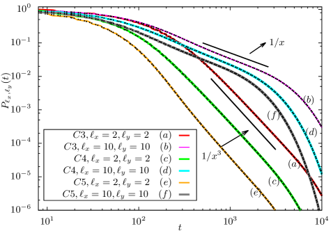
Figure 6: (Color online) Decay of the survival probability $P_{\ell_{x},\ell_{y}}(t)$ for different initial positions $(\ell_{x},\ell_{y})$ of a particle moving on a square lattice of size $N=20$ with different arrangements of the detectors as shown in Fig. 5. C3, C4 and C5 stands for cases (iii), (iv) and (v) respectively. The black dotted lines are the predictions from perturbation theory. The solid black lines are the predicted power law decays for bulk and corner points. (To observe the power law decay for edge points, one needs to choose a large size; this is not shown here.) The measurement time interval was taken to be $\tau=0.1$.

Case (v): Measurement sites placed along all the four boundaries.

The measurement sites are at $(l_{x},1)$ and $(l_{x},N)$, for $l_{x}=1,2,\ldots,N$, and at $(1,l_{y})$ and $(N,l_{y})$, for $l_{y}=2,3,\ldots,N-1$. Then $B_{2D}=B^{\prime}\otimes B^{\prime}$, and

$${\widetilde{U}}_{2D}=\left[B^{\prime}\exp\left(-iHt\right)\right]\otimes\left[B^{\prime}\exp\left(-iHt\right)\right].$$ (32)

When the initial state is $|\phi^{\prime}_{s}\rangle\otimes|\phi^{\prime}_{s^{\prime}}\rangle$, the survival probability is given by

$$P_{s,s^{\prime}}(t)=e^{-(\alpha^{\prime}_{s}+\alpha^{\prime}_{s^{\prime}})t}.$$

When the initial state is $|\ell_{x}\rangle\otimes|\ell_{y}\rangle$, the survival probability is

$$P_{\ell_{x},\ell_{y}}(t) =\sum_{s,s^{\prime}=1}^{N-2}\phi^{\prime 2}_{s}(\ell_{x})\phi^{\prime 2}_{s^{\prime}}(\ell_{y})P_{s,s^{\prime}}(t)$$ (33)

$$=\frac{1}{\sqrt{8\pi x^{\prime}}}[1-e^{-(\ell_{x}-1)^{2}/2x^{\prime}}]~{}$$

$$~{}~{}~{}\times\frac{1}{\sqrt{8\pi x^{\prime}}}[1-e^{-(\ell_{y}-1)^{2}/2x^{\prime}}].~{}$$

This is the product of the survival probabilities of two chains, each with two detectors at the two ends.

To sum up, if the initial state is a position eigenstate, then for cases (i) and (ii), the survival probability decays as $t^{-1/2}$ and $t^{-3/2}$, while for cases (iii), (iv) and (v), it decays as $t^{-1}$, $t^{-3}$, and $t^{-2}$, when the initial position is in the bulk, at the corner (both $x$ and $y$ coordinates are near the ends) or at the edge (one of the coordinates is near the end, and the other is in the bulk) respectively. In Fig. 6 we show the comparison between the analytical predictions for the survival probability for cases (iii), (iv) and (v) using the expressions in Eq. (29), (31) and (33) and the numerical results obtained directly from Eq. (4).

V Exactly solvable mean field model

We now consider the case when a particle can hop to any of the $N$ sites with equal amplitude. Hence the Hamiltonian is

$$H=-\sum_{j,k=1}^{N}|j\rangle\langle k|.$$ (34)

For this case, the Hamiltonian matrix $H$ has all elements equal to $-1$, and one has $e^{-i{H}\tau}=I-{H}/c$ where $c={N}/{(e^{i\tau N}-1)}$. The eigenvalues and eigenvectors of $\widetilde{U}=B~{}(I-H/c)$ are easily found. The eigenvalues are

$$\lambda_{1}=0,\;\;\lambda_{2}=1+(N-1)/c,\;\;\lambda_{s}=1~{}~{}{\rm for}~{}~{}s=3,\ldots,N,$$

(35)

while the corresponding right and left eigenvectors are

$$|R_{1}\rangle =\frac{1}{1-c-N}(1,1,\ldots,1,1-c-N),~{}~{}~{}$$

$$|R_{2}\rangle =\frac{1}{N-1}(1,1,\ldots 1,0),$$

$$|R_{s}\rangle =\frac{1}{N-1}(1,\omega_{s},\omega_{s}^{2}\ldots\omega_{s}^{N-2},0)~{}~{}~{}{\rm for}~{}s=3,\ldots,N,$$

$$\langle L_{1}| =(0,0,\ldots,0,1),~{}~{}~{}~{}\langle L_{2}|=(1,1,\ldots,1,\frac{N-1}{c+N-1}),$$

$$\langle L_{s}| =(1,\omega_{s}^{*},\omega_{s}^{*2},\ldots,\omega_{s}^{*N-2},0)~{}~{}~{}~{}~{}~{}~{}{\rm for}~{}s=3,\ldots,N,$$ (36)

and $\omega_{s}=e^{2\pi i(s-2)/(N-1)}$. Writing $\widetilde{U}=\sum_{s}\lambda_{s}|R_{s}\rangle\langle L_{s}|$, and taking the initial state to be $|\psi(0)\rangle=|\ell\rangle$ (where $\ell\neq N$), we can use Eqs. (5) and (4) to obtain the first detection probability and the survival probability

$$p_{n} =\left|\sum_{s}\langle N|U_{\tau}|R_{s}\rangle~{}\lambda_{s}^{n-1}~{}\langle L_{s}|\ell\rangle\right|^{2}$$

$$=\left|\frac{\lambda_{2}^{n-1}}{c}\right|^{2}=\frac{x}{N-1}\left[1-x\right]^{n-1},$$ (37)

$$P_{n} =1-\frac{1-(1-x)^{n}}{N-1},\;\;\;$$

$${\rm with}~{}~{}~{}x=\frac{2}{N}\left(1-\frac{1}{N}\right)\left(1-\cos\tau N\right)~{}.$$ (38)

For $\ell=N$, we get $p_{1}=1-x,~{}P_{1}=x$ and

$$p_{n} =(N-1)^{2}\left|\frac{\lambda_{2}^{n-2}}{c^{2}}\right|^{2}=x^{2}\left[1-x\right]^{n-2},\;\;\;\;$$

$$P_{n} =x(1-x)^{n}~{},~{}~{}~{}~{}~{}{\rm for}~{}~{}n>1~{}.$$ (39)

For large $N$, one has $x\approx 2(1-\cos\tau N)/N$, and

$$p_{n} = \frac{2e^{\xi}}{N^{2}}\left(1-\cos\tau N\right)e^{-n\xi}~{}~{}~{}\mbox{for ~{}$\ell\neq N$}$$ (40)

$$= \frac{4e^{2\xi}}{N^{2}}\left(1-\cos\tau N\right)e^{-n\xi}~{}~{}\mbox{for $\ell=N$, $n>1$}~{}$$ (41)

where $\xi=\frac{2}{N}\left(1-\cos\tau N\right)$.

Some properties of the first detection probability can be immediately observed:

(1) For $\tau\rightarrow 0$ for a fixed $N$, the probability $p_{n}$ vanishes for all $n$; this is the Zeno effect misra77 ; shimizub05 ; facchi08 ; wineland90 ; kofman ; kwiat ; cirac .

(2) There is a characteristic time $\tau_{0}=2\pi/N$ such that $p_{n}(\tau)=p_{n}(\tau+\tau_{0})$. If we choose $\tau=\tau_{0}\times{\rm integer}$, then $x=0$ according to Eq. (38). For $\ell\neq N$, we then have $p_{n}=0$ for all $n$, while for $\ell=N$, $p_{1}=1$ and $p_{n>1}=0$.

(3) The quantity $p_{n}$ decays exponentially with $n$ for all values of $N$, large or small (see Eqs. (37, 39)).

(4) From Eqs. (37, 39), one can calculate the sum

$$\sum_{n=1}^{\infty}p_{n}=\left\{\begin{array}[]{ll}\frac{1}{N-1}&~{}~{}\mbox{for ~{}$\ell\neq N$}\\ 1&~{}~{}\mbox{for ~{}$\ell=N$}.\end{array}\right.$$ (42)

Thus, if the initial site is different from the detector site then, with a finite probability, the particle is never detected. If we compute the wave function $|\psi^{+}_{n}\rangle$ at large times, we find that it converges to a “steady state” $|\psi_{ss}^{+}\rangle$ with $\langle\ell|\psi^{+}_{ss}\rangle=(N-2)/(N-1)$ and $\langle j|\psi^{+}_{ss}\rangle=-1/(N-1)$ for all $j\neq\ell,N$. This state is invariant under the time evolution, and so we do not see any further decay.

VI Relation to another non-Hermitian Hamiltonian with a large imaginary potential

In Sec. III we showed that the problem of time evolution with a Hermitian Hamiltonian, punctuated by measurements at intervals of time $\tau$, can be related to continuous time evolution with a non-Hermitian Hamiltonian with a small imaginary potential. In this section we show that there also exists a connection to another non-Hermitian Hamiltonian with a large imaginary potential. This then relates our results to the studies in Refs. halliwell10 ; mallick13 .

We will assume that the nearest neighbor hopping amplitude $\gamma$ is the same in the two systems; we will not set $\gamma=1$ in this section. The formalism in Ref. mallick13 contains a non-Hermitian on-site term $-i\gamma\Gamma$ at one site ($\Gamma$ being a dimensionless and positive real number) which leads to a non-unitary evolution. Assuming that $\Gamma\gg 1$ in Ref. mallick13 and $\tau\ll 1/\gamma$ in our formalism, we will develop second order perturbation theory in these quantities and show that the two systems match if $\tau\gamma\Gamma=2$. In a somewhat more general setting of the problem considered in Ref. mallick13 , let us consider the dynamics of a particle evolving with the following Hamiltonian:

$$H_{NH}=H+\Gamma H^{\prime}~{}~{}~{}{\rm{where}}~{}~{}H^{\prime}=-i\gamma\sum_{\alpha\in D}|\alpha\rangle\langle\alpha|~{}$$ (43)

and $H$ is the Hamiltonian defined in Eq. (8). Note that the non-Hermitian Hamiltonian $H_{NH}$ is for the full system, including the sites where measurements are done, unlike the effective non-Hermitian Hamiltonian in Eq. (9). Let us consider the case where $\Gamma$ is large and proceed to compute the spectrum of this non-Hermitian Hamiltonian using perturbation theory.

Let us write the following expansions for the eigenfunctions and eigenvalues of $H_{NH}$:

$$|\Psi\rangle =|\Psi_{0}\rangle+\frac{1}{\Gamma}|\Psi_{1}\rangle+\frac{1}{\Gamma^{2}}|\Psi_{2}\rangle+\ldots,$$

$$E =\Gamma E_{0}+E_{1}+\frac{1}{\Gamma}E_{2}+\ldots~{}.$$ (44)

This leads to the following equations up to second order in perturbation theory:

$$H^{\prime}|\Psi_{0}\rangle =E_{0}|\Psi_{0}\rangle,$$

$$H^{\prime}|\Psi_{1}\rangle+H|\Psi_{0}\rangle =E_{0}|\Psi_{1}\rangle+E_{1}|\Psi_{0}\rangle,$$

$$H^{\prime}|\Psi_{2}\rangle+H|\Psi_{1}\rangle =E_{0}|\Psi_{2}\rangle+E_{1}|\Psi_{1}\rangle+E_{2}|\Psi_{0}\rangle.$$ (45)

At $0^{\rm th}$ order, we see that there are $N_{s}$ degenerate states $|l\rangle$ with eigenvalues $E_{0}=0$, and $N_{D}$ degenerate states $|\alpha\rangle$ with eigenvalues $E_{0}=-i\gamma$. We now examine the corrections to the “system” states at first and second orders in perturbation theory. At first order, the eigenstates are given by $|\Psi_{0}\rangle=\sum_{l}a_{l}|l\rangle,~{}|\Psi_{1}\rangle=\sum_{\alpha}a_{\alpha}|\alpha\rangle$, and the coefficients and energy corrections are given by

$$\sum_{m}H_{l,m}a_{m}=E_{1}a_{l},~{}~{}~{}{\rm where}~{}~{}~{}a_{\alpha}=\frac{1}{i\gamma}\ \sum_{m}V_{\alpha,m}a_{m}.$$ (46)

Assuming, for simplicity, that the states $E_{1}$ are non-degenerate, we see that the second order correction is

$$E_{2} =\langle\Psi_{0}|H|\Psi_{1}\rangle$$

$$=\sum_{l,\alpha}a_{l}a_{\alpha}\langle l|H|\alpha\rangle$$

$$=\sum_{l,m}a_{l}a_{m}\frac{1}{i\gamma}\sum_{\alpha}V_{l,\alpha}V_{\alpha,m}~{}.$$ (47)

Thus we see that the energy levels of the “system” states $E_{1}+E_{2}/\Gamma$ are described by the effective Hamiltonian

$$H_{eff}=H_{S}-\frac{i}{\gamma\Gamma}\sum_{l,m}\sum_{\alpha}V_{l,\alpha}V_{\alpha,m}|l\rangle\langle m|~{}.$$ (48)

We note that this is identical to Eq. (9) with the identification

$$\frac{\tau}{2}=\frac{1}{\gamma\Gamma}~{}.$$ (49)

The quantum survival probability for the particle will therefore match in the two systems if the conditions $\tau<<1/\gamma$ and $\Gamma>>1$ are satisfied, and if Eq. (49) holds.

Earlier in Sec. III we discussed a mapping of the dynamics of the system under repeated measurements to another effective non-Hermitian Hamiltonian. Let us clarify the difference between that and the one discussed in this section, in the context of the special case of a one-dimensional $N$-site chain with open boundary conditions. For this case we have proved that the dynamics under repeated measurements at the $N$-th site at time intervals $\tau$, is identical to the dynamics of both an open chain of $N$ sites with a strong imaginary potential $-i2/\tau$ placed at the $N$-th site (see Eq. (49)) and of an open chain of $(N-1)$ sites with a weak imaginary potential $-i\tau/2$ placed at the $(N-1)$-th site (see Eq. (43) and (10)). A corollary of this observation is that the dynamics of an open $N$-site chain with a strong potential $-iV$ at the $N$-th site is equivalent to that of an open $(N-1)$-site chain with a weak potential $-i/V$ at the $(N-1)$-th site.

VII Discussion

We have used a tight-binding model (with a hopping amplitude $\gamma$) for a particle on a lattice to study the problem of first detection and survival under repeated measurements at a given site or a set of sites. The measurements are made at intervals of time $\tau$. We develop a non-unitary evolution which describes the probability of first detection of the particle at time $t$ and, equivalently, the non-detection or survival of the particle up to the time $t$. We summarize our results below.

Due to the frequent projective measurements made on the system, the wave function evolution is non-unitary. We have shown, using a perturbative approach, that the dynamics can be described by an effective non-Hermitian Hamiltonian, which makes the problem analytically tractable. For a one-dimensional system with either open or periodic boundary conditions and a detector placed at a single site, we derive an analytical expression for the survival probability up to a time $t$ using perturbation theory when $\tau$ is much smaller than the inverse of the band width (proportional to $\gamma$). If $t$ is held fixed, we find that the detection probability vanishes in the limit $\tau\to 0$; this is the quantum Zeno effect. Next, we show that the survival probability generally decays as a power of $t$ for a certain range of values of $t$. The power depends on the initial position of the particle, namely, whether it is near the detecting point or far away from it; we derive an interpolating function which varies from one power law to the other as the initial position is changed. (Interestingly, for periodic boundary conditions, we find that the survival probability generally approaches a non-zero constant as $t\to\infty$). We also find the spatial distribution of the particle when it is not detected and show that it approaches a simple form as $t\to\infty$.

We then consider a number of generalizations of the model. If we consider an open chain with a number of detection points at one end, we find that the system effectively behaves like a shorter open chain with a single detection point at one end. We study an open chain with a detection point at each end and show that the scaling behavior of the survival probability is similar to that of an open chain with one detection point. We have also studied a particle moving on a two-dimensional square lattice. The tight-binding model on this system behaves like a product of two decoupled one-dimensional models in the $x$ and $y$ directions. Hence, the cases in which the detecting sites lie along one edge, two edges (which can be adjacent or opposite to each other), three edges or all four edges, can be mapped to a product of two open chains each of which has a single detecting site at one or both ends. As a result the survival probability and its scaling with time can be derived easily in all these cases. We have then examined a mean field model where the particle can hop between any pair of sites with the same amplitude. In this system, we find that the survival probability is generally finite in the large $t$ limit.

Finally, we have pointed out an interesting connection between our problem and another recent work mallick13 on the survival probability of a particle on a one-dimensional lattice with an imaginary potential at one or more sites. The latter study uses a non-Hermitian and time-independent Hamiltonian in which the potential on a set of sites (which corresponds to the detection sites in our formalism) is imaginary and has a value $-i\gamma\Gamma$; hence the particle can get absorbed there which is the equivalent of getting detected in our language. We show that the two approaches give identical results if $\tau$ is much smaller than the inverse band width $1/\gamma$, $\Gamma\gg 1$, and $\tau\gamma\Gamma=2$.

We can consider various extensions of this work for future studies. It may be interesting to look at many-body systems and investigate the effect of repeated measurements at one point on the particle distribution near that point and to see if measurements can give rise to quantum entanglement. It would also be interesting to look at the effect of measurements of observables other than the position, such as the momentum or the spin.

Acknowledgments

S. Dhar gratefully acknowledges CSIR, India for providing a research fellowship through sanction no. 09/028(0839)/2011-EMR-I. The work of S. Dasgupta is supported by UGC-UPE (University of Calcutta). S. Dasgupta is also grateful to ICTS, Bangalore for hospitality. AD thanks DST, India for support through the Swarnajayanti grant. DS thanks DST, India for Project No. SR/S2/JCB-44/2010.

References

- (1) G. R. Allcock, Ann. of Phys. 53, 253 (1969); G. R. Allcock, Ann. of Phys. 53, 286 (1969).
- (2) J. Kijowski, Rep. Math. Phys. 6, 361 (1974).
- (3) N. Kumar, Pramana-J. Phys 25, 363 (1985).
- (4) N. Grot, C. Rovelli, and R. S. Tate, Phys. Rev. A 54, 4676 (1996).
- (5) Y. Aharonov, J. Oppenheim, S. Popescu, B. Reznik, and W. G. Unruh, Phys. Rev. A 57, 4130 (1998).
- (6) C. Anastopoulos and N. Savvidou, J. Math. Phys. 47, 122106 (2006).
- (7) J. G. Muga, A. D. Baute, J. A. Damborenea, and I. L. Egusquiza, arXiv:quant-ph/0009111 (2000).
- (8) J. A. Damborenea, I. L. Egusquiza, G. C. Hegerfeldt, and J. G. Muga, Phys. Rev. A 66, 052104 (2002).
- (9) E. A. Galapon, R. F. Caballar, and R. T. Bahague Jr, Phys. Rev. Lett. 93, 180406 (2004).
- (10) E. A. Galapon, F. Delgado, J. G. Muga, and I. Egusquiza, Phys. Rev. A 72, 042107 (2005).
- (11) J. Echanobe, A. del Campo, and J. G. Muga, Phys. Rev. A 77, 032112 (2008).
- (12) J. M. Yearsley, D. A. Downs, J. J. Halliwell, and A. K. Hashagen, Phys. Rev. A 84, 022109 (2011).
- (13) C. Anastopoulos and N. Savvidou, Phys. Rev. A 86, 012111 (2012).
- (14) N. Vona, G. Hinrichs, and D. Dürr, Phys. Rev. Lett. 111, 220404 (2013).
- (15) J. G. Muga and C. R. Leavens, Phys. Rep. 338, 353 (2000).
- (16) G. Torres-Vega, Phys. Rev A, 76, 032105 (2007).
- (17) G. Torres-Vega, J. Phys. A: Math. Theor. 42, 465307 (2009).
- (18) B. Mielnik and G. Torres-Vega, Concepts of Physics 2 , 81 (2005), arXiv:1112.4198v1[quant-ph].
- (19) B. Misra and E. C. G. Sudarshan, J. Math. Phys. 18, 756 (1977).
- (20) K. Koshino and A. Shimizu, Phys. Rep. 412, 191 (2005).
- (21) P. Facchi and S. Pascazio, J. Phys. A 41, 493001 (2008).
- (22) W. M. Itano, D. J. Heinzen, J. J. Bollinger, and D. J. Wineland, Phys. Rev. A 41, 2295 (1990).
- (23) A. G. Kofman and G. Kurizki, Phys. Rev. A 54, R3750 (1996).
- (24) P. G. Kwiat, A. G. White, J. R. Mitchell, O. Nairz, G. Weihs, H. Weinfurter, and A. Zeilinger, Phys. Rev. Lett. 83, 4725 (1999).
- (25) J. I. Cirac, A. Schenzle, and P. Zoller, Euro. Phys. Lett. 27, 123 (1994).
- (26) W. M. Itano, J. Phys.: Conf. Series, 196, 012018 (2009).
- (27) A. Signoles, A. Facon, D. Grosso, I. Dotsenko, S. Haroche, J.-M. Raimond, M. Brune, and S. Gleyzes, Nature Physics 10, 715 (2014).
- (28) G. C. Hegerfeldt and D. G. Sondermann, Quant. Semiclassic. Opt. 8, 121 (1996).
- (29) N. Erez, G. Gordon, M. Nest, and G. Kurizki, Nature 452, 724 (2008).
- (30) T. Jahnke and G. Mahler, Euro. Phys. Lett. 90, 50008 (2010).
- (31) C. O. Bretschneider, G. A. Álvarez, G. Kurizki, and L. Frydman, Phys. Rev. Lett. 108, 140403 (2012).
- (32) J. J. Halliwell and J. M. Yearsley, J. Phys. A 43, 445303 (2010).
- (33) J. Yi, P. Talkner, and G.-L. Ingold, Phys. Rev. A 84, 032121 (2011).
- (34) S. Dhar, S. Dasgupta, and A. Dhar, J. Phys. A: Math. Theor. 48, 115304 (2015).
- (35) P. L. Krapivsky, J. M. Luck, and K. Mallick, J. Stat. Phys. 154, 1430 (2014).