Correlated Quantum Dynamics of a Single Atom Collisionally Coupled to an Ultracold Finite Bosonic Ensemble

Abstract

We explore the correlated quantum dynamics of a single atom, regarded as an open system, with a spatio-temporally localized coupling to a finite bosonic environment. The single atom, initially prepared in a coherent state of low energy, oscillates in a one-dimensional harmonic trap and thereby periodically penetrates an interacting ensemble of $N_{A}$ bosons, held in a displaced trap. We show that the inter-species energy transfer accelerates with increasing $N_{A}$ and becomes less complete at the same time. System-environment correlations prove to be significant except for times when the excess energy distribution among the subsystems is highly imbalanced. These correlations result in incoherent energy transfer processes, which accelerate the early energy donation of the single atom and stochastically favour certain energy transfer channels depending on the instantaneous direction of transfer. Concerning the subsystem states, the energy transfer is mediated by non-coherent states of the single atom and manifests itself in singlet and doublet excitations in the finite bosonic environment. These comprehensive insights into the non-equilibrium quantum dynamics of an open system are gained by ab-initio simulations of the total system with the recently developed Multi-Layer Multi-Configuration Time-Dependent Hartree Method for Bosons.

1 Introduction

Many physically relevant quantum systems are in fact open. Intriguing effects in e.g. condensed matter physics [1], quantum optics [2], molecules or light harvesting complexes [3, 4, 5] are intimately related to environmentally induced dissipation and decoherence and thus require a careful treatment beyond the unitary dynamics of the time-dependent Schrödinger equation. As one can often neither experimentally control nor theoretically describe all the environmental degrees of freedom, a variety of theoretical methods has been developed for an effective description of the reduced dynamics of the open quantum system of interest over the last decades [6].

Due to their high degree of controllability and, in particular, isolatedness [7], ensembles of ultracold atoms or ions serve as ideal systems in order to systematically study the dynamics of open quantum systems allowing for various perspectives on this subject [8]. Open quantum system dynamics has been implemented by digital quantum simulators [9, 10] or by partitioning an ultracold atomic ensemble into carefully coupled, distinguishable subsystems [11]. As a matter of fact, many impurity problems can also be viewed as open quantum system settings: enormous experimental progress such as [12, 13, 14, 15] allows to prepare a few impurities or even a single one in an ensemble of atoms in order to study thermalization and atom loss mechanisms [16], transport and polaron physics [17, 18, 19] or the damping of the breathing mode [20, 21]. Such implementations of open quantum systems offer the unique flexibility to tune both the character and strength of the system-environment coupling [20] and the environmental properties [19]. Moreover, dissipation and environment engineering can also be employed for controlling many-body dynamics [22], state preparation [23] as well as quantum computation [24, 25].

In this work, we theoretically study the open quantum system dynamics of a single atom with a weak spatio-temporally localized coupling to a finite bosonic environment, focusing in particular on the characterization of the inter-species energy transfer processes. By considering a binary mixture of neutral atoms interacting via contact interaction both within and between the species, the local character of the coupling is realized. In order to localize the coupling also in time, species-selective one-dimensional trapping potentials as well as a particular initial condition are considered: the single atom is initially displaced from the centre of its harmonic trap, i.e. resides in a coherent state, while the bosonic ensemble is prepared in the ground state of a harmonic trapping potential being shifted from the trap of the single atom. Thereby, both subsystems couple only during a certain phase of the single atom oscillation and the effective coupling strength becomes strongly dependent on the instantaneous subsystem states. In a different context, this kind of coupling has already been realized effectively experimentally [26]. The basic ingredient of such a coupling, a single binary collision, can result in entanglement between the collision partners [27, 28, 29, 30], which has been shown to depend on the details such as the scattering phase shift, the mass ratio as well as the relative momentum of the atoms [31]. As a consequence, significant correlations between the single atom and the finite bosonic environment can occur after many collisions despite of possibly weak interactions (cf. also [28, 32, 33] in this context), undermining a mean-field approximation for the two species on a longer time scale. We note that the scenario under consideration might seem to be reminiscent of the quantum Newton’s cradle [34, 35, 36]. Yet instead of investigating the (absence of) thermalization in a closed system of indistinguishable constituents, we are concerned with unravelling the interplay of energy transfer between distinguishable subsystems and the emergence of correlations when systematically increasing the number of environmental degrees of freedom $N_{A}$.

Rather than simulating the reduced dynamics of the single atom only, we employ the recently developed ab-initio Multi-Layer Multi-Configuration Time-Dependent Hartree Method for Bosons (ML-MCTDHB) [37, 38] for obtaining the non-equilibrium quantum dynamics of the whole system for various numbers of environmental degrees of freedom. Such a closed system perspective on an open quantum system problem gives the unique opportunity to investigate not only the dynamics of the open system but also its impact on the environment and, moreover, to systematically uncover correlations between the two subsystems (cf. also e.g. [39, 40]). Full numerical simulations are supplemented with analytical and perturbative considerations.

This paper is organized as follows: In sect. 2, we introduce our setup and discuss a possible experimental implementation. Moreover, we argue how the inter-species energy transfer channels can be controlled by appropriately tuning the separation of the involved species-selective traps. The subsequent sect. 3 is devoted to the energy transfer dynamics between the single atom and the finite bosonic environment. Here, we show that the energy transfer between the subsystems is accelerated with increasing $N_{A}$ due to a level splitting of the involved excited many-body states. On top of it, the relative amount of the total energy being exchanged between the subsystems is reduced when increasing $N_{A}$. After an initial slip the energy distribution among the subsystems consequently fluctuates about quite a balanced one for larger $N_{A}$. In sect. 4, we investigate how the subsystem states are affected by the system-environment coupling: By inspecting the Husimi phase space distribution of the single atom, we conclude that the energy transfer is mediated by non-coherent states manifesting themselves in a drastic deformation of the phase space distribution during relatively short time slots. Concerning the environment, depletion oscillations are observed, whose amplitude decreases with increasing $N_{A}$ when fixing the initial displacement of the single atom. In sect. 5, we unravel the oscillatory emergence and decay of inter-species correlations showing that whenever the excess energy distribution among the subsystems is highly imbalanced, correlations have to be strongly suppressed. The maximal attained correlations turn out to be independent of the considered number of environmental degrees of freedom $N_{A}$. By analysing the subsystem energy distribution among the so-called natural orbitals, we show how inter-species correlations result in incoherent energy transfer processes, which accelerate the early energy donation of the single atom. Most importantly, we ultimately uncover the interplay between subsystem excitations and correlations by means of a Fock space excitation analysis in sect. 6, characterizing the environmental excitations and unravelling correlations between subsystem excitations with a tailored correlation measure. Thereby, we can show that inter-species correlations (dis-)favour certain energy transfer channels depending on the instantaneous direction of transfer in general. Finally, we conclude and give an outlook in sect. 7.

2 Setup and initial conditions

The subject of this work is a bipartite system confined to a single spatial dimension and consisting of two atomic species: a single atom is collisionally coupled to a finite bosonic environment (cf. fig. 1 (c)). We model the intra- and inter-species short-range interactions with a contact potential as it is usually done in the ultracold s-wave scattering limit [41]. In addition, we assume two external harmonic potentials for a species-selective trapping of the atoms. In the following, we adopt a shorthand notation labelling the bosonic environment with $A$ and the single atom with $B$. Throughout this work, all quantities are given in terms of natural harmonic oscillator units of $B$, which base on the mass of the single atom $m_{B}$ and its trapping frequency $\omega_{B}$. Lengths, energies and times are thus given in terms of $\sqrt{\hbar/(m_{B}\omega_{B})}$, $\hbar\omega_{B}$ and $\omega_{B}^{-1}$, respectively. The Hamiltonian of the composite system takes the form

$$\hat{H}=\hat{H}_{A}+\hat{H}_{B}+\hat{H}_{AB}$$ (1)

with the Hamiltonian of the environment $\hat{H}_{A}$, the open system $\hat{H}_{B}$ and the inter-subsystem coupling $\hat{H}_{AB}$:

$$\hat{H}_{A} =\sum_{i=1}^{N_{A}}\left(\frac{1}{2\beta}({\hat{p}^{A}_{i}})^{2}+\frac{\alpha^{2}\beta}{2}(\hat{x}^{A}_{i}+R)^{2}\right)+g_{A}\sum_{1\leq i<j\leq N_{A}}\delta(\hat{x}^{A}_{i}-\hat{x}^{A}_{j}),$$

$$\hat{H}_{B} =\frac{1}{2}({\hat{p}^{B}})^{2}+\frac{1}{2}(\hat{x}^{B})^{2},$$ (2)

$$\hat{H}_{AB} =g_{AB}\sum_{k=1}^{N_{A}}\delta(\hat{x}^{B}-\hat{x}^{A}_{k}).$$

The dimensionless representation of the Hamiltonian involves the mass ratio $\beta=m_{A}/m_{B}$ and the frequency ratio $\alpha=\omega_{A}/\omega_{B}$. $R>0$ denotes the separation between the traps and the intra- and inter-species interaction strengths are given by $g_{A}$ and $g_{AB}$, respectively. We emphasize that the variety of parameters specifying the Hamiltonian (1) accounts for the versatility of the considered system, which to explore in its complexity goes far beyond this work. Rather than this, we fix $g_{A},g_{AB}$ to experimentally feasible values by considering two ⁸⁷Rb hyperfine states of comparable intra- and inter-species scattering lengths, implying $\beta=1$. Assuming $\omega_{B}=10\,{\rm Hz}$ and a transverse to longitudinal trapping frequency ratio of about $68$ for both species, we are left with $g_{A}=g_{AB}=0.08$ for the one-dimensional coupling constants after dimensional reduction [42, 43].

\begin{overpic}[width=346.89731pt]{exp_proposal_sketch.png} \put(0.0,96.0){(a)} \put(0.0,62.0){(b)} \put(0.0,29.0){(c)} \put(5.0,87.0){\color[rgb]{0,0,1}{$m_{F}=-1$}} \put(5.0,50.0){\color[rgb]{0,0,1}{$m_{F}=-1$}} \put(5.0,18.0){\color[rgb]{0,0,1}{$m_{F}=-1$}} \par\put(83.0,87.0){\color[rgb]{1,0,0}{$m_{F}=1$}} \put(83.0,50.0){\color[rgb]{1,0,0}{$m_{F}=1$}} \put(83.0,18.0){\color[rgb]{0.0,0.5,0.0}{$m_{F}=0$}} \put(90.0,42.0){$B(x)$} \put(95.0,6.0){$x$} \put(33.0,33.0){\tiny{spatio-temporally}} \put(33.0,31.0){\tiny{localized coupling}} \put(38.0,25.0){$g_{AB}$} \put(33.0,16.0){$N_{A}$} \put(60.0,30.0){$N_{B}=1$} \put(34.0,12.0){$g_{A}$} \put(32.0,4.0){$-R$} \put(50.25,4.0){$0$} \put(66.0,4.0){$d$} \end{overpic}

Figure 1: Sketch of a possible three-step realization of the bipartite system with the single atom initially prepared in a coherent state. (a) An optical dipole trap holds $N_{A}$ atoms ($m_{F}=-1$) and a single impurity atom ($m_{F}=+1$). (b) Application of an external magnetic field gradient yields a spatial separation of the ensemble and the impurity. (c) A RF field drives the $m_{F}=1$ to $m_{F}=0$ transition and initializes the single atom in a displaced ground state.

We initialize $B$ in a coherent state $\ket{z}$:

$$\ket{z}=e^{-|z|^{2}/2}\sum_{n=0}^{\infty}\frac{z^{n}}{\sqrt{n!}}\ket{u^{B}_{n}}$$ (3)

where $\ket{u^{\sigma}_{n}}$ denotes the $n^{th}$ harmonic oscillator (HO) eigenfunction of the species $\sigma=A,B$ with energy $E^{A}_{n}=\alpha(1/2+n)$, $E^{B}_{n}=E^{A}_{n}/\alpha$, respectively. We choose $z=d/\sqrt{2}>0$ such that $\ket{z}$ equals the $\hat{H}_{B}$ ground state displaced by a distance $d$ to the right from the $B$ species trap centre. The environment, $A$, in turn is prepared in the ground state of $\hat{H}_{A}$. In order to realize the desired spatio-temporally localized coupling, whose impact on the inter-species energy transfer and emergence of correlations shall be investigated, we require $R$ and $d$ to be such that there is (i) no inter-species overlap at $t=0$ and (ii) finite overlap after half of a $B$ atom oscillation period, i.e. at $t\approx\pi$. For more details on the initial state preparation and subsequent propagation with our ab-initio ML-MCTDHB method, see A and B.

In order to characterize the spatio-temporally localized coupling, we express $\hat{H}_{AB}$ in terms of the HO eigenbasis $\left\{|u^{\sigma}_{n}\rangle\right\}$, which serves as a natural choice for the low-energy and weak-coupling regime we are interested in,

$$\hat{H}_{AB}=g_{AB}\sum_{i,j,p,q}v_{ijpq}{\hat{a}}^{\dagger}_{i}{\hat{a}}_{p}\otimes|u^{B}_{j}\rangle\!\langle u^{B}_{q}|,$$ (4)

with $\hat{a}^{(\dagger)}_{i}$ denoting the bosonic annihilation (creation) operator corresponding to $|u^{A}_{i}\rangle$ and the interaction-matrix elements given by

$$v_{ijpq} =\braket{u^{A}_{i}u^{B}_{j}}{\delta(\hat{x}^{A}-\hat{x}^{B})}{u^{A}_{p}u^{B}_{q}}=\int_{-\infty}^{+\infty}dx\ [u_{i}^{A}(x)u^{B}_{j}(x)]^{*}u^{A}_{p}(x)u^{B}_{q}(x),$$ (5)

which obviously depends on $\alpha$ and $R$. Eventually, we are interested in rather small displacements $d$ for which the matrix element $v_{1001}$ is of major importance for the dynamics. For e.g. $\alpha=1$, we find that $v_{1001}=(1-R^{2})\exp(-R^{2}/2)/(2\sqrt{2\pi})$. Hence, the scattering channels "$\ket{u_{0}^{A}}\ket{u_{1}^{B}}\leftrightarrow\ket{u_{1}^{A}}\ket{u_{0}^{B}}$" are completely suppressed at $R=1$. In order to avoid artefacts of such selection rules, we choose $R=1.2$, for which the relevant low-energy scattering channels are not suppressed.

Although we have fixed some of the parameters, the system still features a high sensitivity to $\alpha$, $d$, $N_{A}$ and thus controllability. For $N_{A}=1$, analytical expressions for the energy spectrum and the wave functions can be worked out and trap-induced shape resonances between molecular and trap states are detectable [44, 45]. Since this two-body problem has already been treated in detail, we shall rather focus on the impact of the environment size, considering $N_{A}=2,...,10$.

Finally, we briefly comment on an experimental realization of this open quantum system problem. Having loaded an ensemble of ${|F=1,m_{F}=-1\rangle}$ polarized ⁸⁷Rb atoms in an optical dipole trap with a deep transverse optical lattice, the site-selective spin flip technique based on an additional longitudinal pinning lattice [14] or the doping technique in [16] allows for creating a single $|F=1,m_{F}=1\rangle$ impurity (fig. 1 (a)). By adiabatically ramping up a longitudinal magnetic field gradient, the species are spatially displaced in opposite directions (fig. 1 (b)). Then the $m_{F}=1$ to $m_{F}=0$ transition can be selectively addressed by a RF field using the quadratic Zeeman effect such that the single $B$ atom ($m_{F}=0$) is initialized in a displaced coherent state, realizing $d=R$ and $\alpha=1$ (fig. 1 (c)). The energy of the $B$ atom can be inferred from its oscillation turning points via in situ density [12, 13] or tunnelling measurements [46].

3 Energy transfer

In order to understand which kind of energy transfer processes between the species are feasible with the spatio-temporally localized coupling and how efficient these are, we examine the energies of the subsystems, identified with $\braket{\hat{H}_{A}}_{t}$ and $\braket{\hat{H}_{B}}_{t}$, separately. Since the interaction energy $\braket{\hat{H}_{AB}}_{t}$ cannot be attributed to the energy content of a single species, the aforementioned identification is problematic, in general. However, the spatio-temporally localized coupling always allows to find times during a $B$ atom oscillation at which the inter-species interaction is essentially negligible so that $\braket{\hat{H}_{A}}_{t}$ and $\braket{\hat{H}_{B}}_{t}$ then measure how the energy is distributed among the open system and its environment. Because of the weak and spatio-temporally localized inter-species coupling, the short-time dynamics taking place on the time-scale of the free oscillation period of the $B$ atom, i.e. $T=2\pi$, is clearly separated from the long-time dynamics of the energy transfer between the two species. When quantifying times, we will use the term “$B$ oscillations” always with reference to free harmonic oscillations of the $B$ atom. Due to this time-scale separation, we present the expectation value of any physical observable $\hat{O}$ as locally time-averaged over one free $B$ oscillation period,

$$\bar{O}(t)=\frac{1}{2\pi}\int_{t}^{t+2\pi}d\tau\braket{\Psi_{t}}{\hat{O}}{\Psi_{t}}.$$ (6)

Thereby, we average out fluctuations on the short time-scale of a $B$ oscillation, giving a clearer view on the long-time dynamics. The fast short-time dynamics is captured by the variance of the local time-average,

$${\rm var}(\hat{O};t)=\frac{1}{2\pi}\int_{t}^{t+2\pi}d\tau\braket{\Psi_{\tau}}{\hat{O}^{2}}{\Psi_{\tau}}-\bar{O}_{t}^{2}.$$ (7)

In some cases, it turns out to be insightful to encode this information in the figures by accompanying the lines corresponding to $\bar{O}(t)$ with a shaded area indicating the standard deviation.

We prepare the system such that the two species have no spatial overlap at $t=0$. Therefore, the initial energy of the single atom reads

$$\langle\hat{H}_{B}\rangle_{t=0}=\frac{d^{2}+1}{2}.$$ (8)

By adjusting the displacement $d$, we can thus vary the amount of deposited excess energy $\varepsilon\equiv d^{2}/2$, which is available for energy transfer processes between the subsystems. These energy transfer processes are captured in terms of the intra-species excess energies $\varepsilon^{\sigma}_{t}=\langle\hat{H}_{\sigma}\rangle_{t}-E^{\sigma}_{\rm gs}$ with $E^{\sigma}_{\rm gs}$ denoting the ground state energy of $\hat{H}_{\sigma}$, $\sigma=A,B$. We employ the normalized excess energy of $B$, $\Delta^{B}_{t}=\varepsilon^{B}_{t}/\varepsilon$, in order to measure how balanced the deposited energy is distributed among the subsystems: At instants for which $\langle\hat{H}_{AB}\rangle_{t}$ is negligible, one obviously finds $\varepsilon^{A}_{t}/\varepsilon=1-\Delta^{B}_{t}$. Thus $\Delta^{B}_{t}\approx 1(0)$ implies then that almost all excess energy is stored in the $B$ ($A$) species, corresponding to a maximally imbalanced excess energy distribution, while $\Delta^{B}_{t}\approx 0.5$ refers to a balanced distribution. Due to the initial imbalance $\Delta^{B}_{0}=1$, the $B$ atom will first donate energy to its environment implying an overall decrease of $\Delta^{B}_{t}$ until $\Delta^{B}_{t}$ reaches a minimum. We call the energy donation of $B$ the more efficient the closer to zero this minimum is. Afterwards, the $B$ atom will generically accept energy from its environment, resulting in an overall increase of $\Delta^{B}_{t}$ until it reaches a maximum. We call such an energy transfer cycle the more complete the closer to unity this maximum is.

First of all, we investigate how the geometric properties of the trap and the initial excess energy influence the energy donation by inspecting $\max_{t}(1-\Delta^{B}_{t})$ for various values of $d\in[0.5,3]$ and $\alpha\in[2/3,4/3]$ and for a fixed, reasonably long propagation time. While the maximal fraction of excess energy transferred to the A species is rather independent of d, we observe a sharp resonance at $\alpha=1$ (plot not shown). As we will show (cf. D), intriguing open-quantum system dynamics with a significant impact of inter-species correlations can only take place for excess energies $\varepsilon$ being at least of the order of the excitation gap of $\hat{H}_{A}$, which equals $\alpha$ when neglecting the intra-species interactions. In this work, we thus concentrate on the resonant case $\alpha=1$ with $\varepsilon\approx\alpha$ so that not too many scattering channels are energetically open, which paves the way for a thorough understanding of the dynamics. If not stated otherwise, $d=1.5$ is consequently assumed leaving us with $N_{A}$ as the only free parameter.

Fig. 2 shows the normalized excess energy $\bar{\Delta}^{B}(t)$ for $N_{A}=2,4,7,10$. As a starting point, we discuss the case $N_{A}=2$. The initial excess energy distribution is maximally imbalanced, i.e. $\Delta^{B}_{t=0}=1$. As $B$ donates energy to its environment, $\bar{\Delta}^{B}(t)$ monotonously decreases until reaching a global minimum at $t\approx 289$, implying a directed energy transfer from $B$ to $A$. The energy transfer decelerates at $t\approx 145$ and reaccelerates at $t\approx 190$. When $\bar{\Delta}^{B}(t)$ attains its minimum at $t\approx 289$, the reverse energy transfer process is initiated and $B$ accepts the energy that was donated to $A$ in the first place. Decelerated energy transfer can also be observed between $t\approx 395$ and $t\approx 440$. At $t\approx 584$, $\bar{\Delta}^{B}(t)$ attains a local maximum and the excess energy is almost completely restored in $B$ ($\bar{H}_{B}(t=584)\gtrsim 0.97\braket{\hat{H}_{B}}(t=0)$).

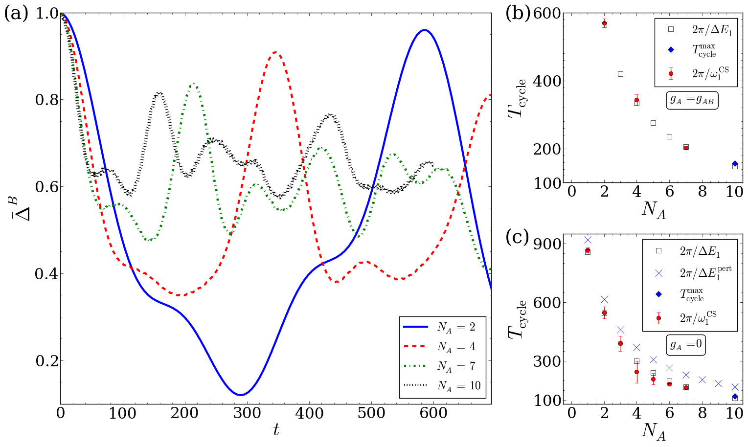
Figure 2: (a) Evolution of the excess energy imbalance $\bar{\Delta}^{B}(t)$ for various $N_{A}$. (b) Time-scale $T_{\rm cycle}=2\pi/\omega_{1}^{\rm CS}$ of an energy transfer cycle obtained by compressed sensing of $\langle\hat{H}_{B}\rangle_{t}$ simulation data (full circles, error bars indicate the standard deviation related to the corresponding peak width in the frequency spectrum). For $N_{A}=10$, we provide the instant $T_{\rm cycle}^{\rm max}$ of the first significant $\bar{\Delta}^{B}(t)$ maximum besides $t=0$ (blue diamond) instead of $2\pi/\omega_{1}^{\rm CS}$. Squares denote the time-scale $2\pi/\Delta E_{1}$ induced by the level spacing $\Delta E_{1}$ of the first excited manifold calculated with ML-MCTDHB. (c) Same as (b) but for $g_{A}=0$. Crosses refer to the time-scale $2\pi/\Delta E_{1}^{\rm pert}$ with $\Delta E_{1}^{\rm pert}$ denoting the first order perturbation theory approximation for $\Delta E_{1}$. Other parameters: $\alpha=1$, $d=1.5$. All quantities in HO units of $\hat{H}_{B}$.

Now we turn to the impact of $N_{A}$ on $\bar{\Delta}^{B}(t)$. The oscillatory evolution of $\bar{\Delta}^{B}(t)$ is similar for $N_{A}=2$ and $N_{A}=4,7,10$. For example, we identify the minimum of $\bar{\Delta}^{B}(t)$ for $N_{A}=2$ at $t\approx 289$ with the minimum of $\bar{\Delta}^{B}(t)$ for $N_{A}=4$ at $t\approx 195$. Analogously, the maximum of $\bar{\Delta}^{B}(t)$ for $N_{A}=2$ at $t\approx 584$ indicating that $B$ accepted much of the excess energy $\varepsilon$ from the environment corresponds to the maximum of $\bar{\Delta}^{B}(t)$ for $N_{A}=4$ at $t\approx 345$. Already after a few $B$ oscillations, $\bar{\Delta}^{B}(t)$ is considerably smaller for higher $N_{A}$ than for $N_{A}=2$. Thus, all results shown in fig. 2 indicate that the overall energy transfer process accelerates with increasing $N_{A}$. Classically, this can be understood in terms of an increasing number of collision partners, making excitations in $A$ more likely to occur within a $B$ oscillation. This manifests itself in the effective mean-field coupling strength $g_{AB}N_{A}$. For a quantum-mechanical explanation, we firstly extract the energy transfer time-scale $T_{\rm cycle}$ by applying compressed sensing [47, 48] to the $\langle\hat{H}_{B}\rangle_{t}$ data, which gives an accurate, sparse frequency spectrum despite of the short signal length. In fig. 2 (b), we depict $T_{\rm cycle}=2\pi/\omega_{1}^{\rm CS}$ with $\omega_{1}^{\rm CS}$ denoting the angular frequency of the dominant peak aside from the DC peak at zero frequency. For $N_{A}=10$ however, the compressed sensing spectrum is relatively smeared out such that $\omega_{1}^{\rm CS}$ cannot reliably be determined. This effect is probably caused by dephasing of various populated many-body eigenstates of $\hat{H}$ and so we estimate $T_{\rm cycle}$ by the first instant $T_{\rm cycle}^{\rm max}>0$ when $\bar{\Delta}^{B}(t)$ attains a significant local maximum. We observe excellent agreement of $T_{\rm cycle}$ with the time-scale $2\pi/\Delta E_{1}$ induced by the energy gap $\Delta E_{1}$ between the first and second excited many-body eigenstate of $\hat{H}$ obtained with ML-MCTDHB (cf. A). In order to obtain a pictorial understanding of the $\Delta E_{1}$ increase with $N_{A}$, we have repeated our analysis for the case $g_{A}=0$, allowing for the analytical expression $\Delta E_{1}^{\rm pert}=g_{AB}[(N_{A}-1)^{2}(v_{1010}-v_{0000})^{2}-4N_{A}v_{1001}^{2}]^{\frac{1}{2}}$ for the level spacing $\Delta E_{1}$ within first-order degenerate perturbation theory w.r.t. $\hat{H}_{AB}$. This perturbative result is in qualitative agreement with the numerics in fig. 2 (c). Denoting $|n_{0},n_{1},...\rangle^{A}_{\rm HO}$ as a bosonic number state with $n_{i}$ atoms of type $A$ occupying $|u_{i}^{A}\rangle$, the following mechanism becomes immediately clear: While for the unperturbed state $|N_{A},0\rangle^{A}_{\rm HO}\otimes|u^{B}_{1}\rangle$ a fraction of the $B$ atom wave function leaks more strongly into the ensemble of $N_{A}$ bosons, for the unperturbed state $|N_{A}-1,1\rangle^{A}_{\rm HO}\otimes|u^{B}_{0}\rangle$ only a single $A$ boson more significantly leaks into the region where the $B$ is located. Thus, the inter-species interaction raises the former state more in energy than the latter and thereby splits the degeneracy of these states. Since we consider small bosonic ensembles and a weak intra-species interaction strength, this explanation for the energy transfer acceleration with $N_{A}$ holds also for $g_{A}=g_{AB}$ in good approximation.

Moreover, the results shown in fig. 2 (a) for $N_{A}>2$ feature less pronounced energy minima and maxima. In our terminology, the energy donation becomes less efficient and the whole transfer cycle less complete as $N_{A}$ is increased. For $N_{A}\geq 7$, this culminates in the following behaviour: After the initial time period of energy donation from $B$ to $A$ lasting a few tens of $B$ oscillations, $\bar{\Delta}^{B}(t)$ fluctuates around the value for a balanced distribution, i.e. $\sim 0.6...0.65$. We note that the above mentioned time periods of decelerated energy transfer are not observed for $N_{A}>4$. Instead, additional structure emerges in the form of not only deceleration but a short time period in which $B$ accepts energy, see e.g. the additional local minimum and maximum for $N_{A}=7$ at $t\approx 70$ and $t\approx 100$, respectively.

4 State analysis of the subsystems

In this chapter, we aim at a pictorial understanding of the subsystem dynamics. For this purpose, we study the impact of the spatio-temporarily localized coupling on the short time-evolution of the $B$ atom density and the reduced one-body density of the $A$ species (sect. 4.1). Afterwards, we employ the Husimi phase-space representation of the state of $B$ for investigating to which extent its initial coherence is affected by the environment (sect. 4.2). Likewise, we shall also characterize the environment whilst inspecting its depletion from a perfectly condensed state (sect. 4.3). Further insights into the environmental dynamics are given in sect. 6.2 focusing on intra-species excitations.

4.1 One-body densities

Any predictions about measurements upon the single $B$ atom alone can be inferred from its reduced density operator $\hat{\rho}^{B}_{t}$, which is thus regarded as the state of the $B$ atom:

$$\hat{\rho}^{B}_{t}=\tr_{A}|\Psi_{t}\rangle\!\langle\Psi_{t}|.$$ (9)

Here, $\tr_{A}$ denotes a partial trace over all $A$ bosons. Analogously, we define $\hat{\rho}^{A}_{t}$ as a partial trace over the $B$ atom and all $A$ bosons but one.

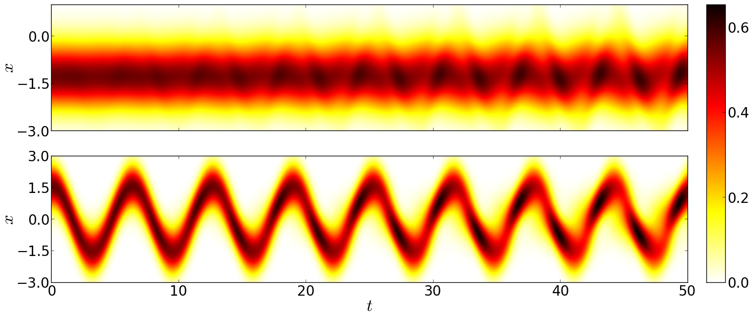
Figure 3: One-body densities $\rho^{\sigma}_{t}(x)$ for the $\sigma=A$ ($B$) species in the upper (lower) panel during the first eight B oscillations. System parameters: $N_{A}=2$, $\alpha=1$, $d=1.5$. All quantities in HO units of $\hat{H}_{B}$.

Due to inter-species interactions, the single atom leaves a trace in the spatial density profile of $A$. Fig. 3 shows the reduced densities, $\rho^{\sigma}_{t}(x)=\braket{x}{\hat{\rho}^{\sigma}_{t}}{x}$ with $\sigma=A,B$, for the first eight oscillations of $B$. It mediates a rather intuitive picture of the process that takes place: $B$ initiates oscillatory density modulations in $A$ via two-particle collisions emerging already after a few $B$ oscillations. The single atom experiences a back action from $A$ in terms of oscillations between spatio-temporally localized and smeared out $\rho_{t}^{B}(x)$ density patterns.

4.2 Coherence analysis

However, the spatial density yields no information about how coherent the state $\hat{\rho}^{B}_{t}$ of the single atom remains. Instead, the Husimi distribution

$$Q^{B}_{t}(z,z^{*})=\frac{1}{\pi}\braket{z}{\hat{\rho}^{B}_{t}}{z},\quad z\in\mathbb{C},$$ (10)

serves as a natural quantity to unravel deviations from a coherent state characterized by an isotropic Gaussian distribution. Due to its positive-semi-definiteness, $Q^{B}_{t}(z,z^{*})$ allows for an interpretation as the probability density to find the system in the coherent state $\ket{z}$. The real and imaginary parts of $z\equiv re^{i\varphi}$ can be identified with position and momentum in a phase space representation, i.e. $\Re(z)=\tilde{x}/\sqrt{2},\ \Im(z)=\tilde{p}/\sqrt{2}$.

Since $B$ performs harmonic oscillations in its trap, which entail rotations of $Q^{B}_{t}$ in phase space, the subsequent phase space analysis is performed in the co-rotating frame of $B$ in terms of $\tilde{Q}^{B}_{t}(z,z^{*})\equiv Q^{B}_{t}(ze^{-it},z^{*}e^{it})$. In fig. 4 (a), $\bar{\Delta}^{B}(t)$ is shown as well as snapshots of $\tilde{Q}^{B}_{t}(z,z^{*})$ at characteristic points in time for $N_{A}=2$ and $d=1.5,2.5$. The initial Husimi distributions are Gaussians centred around $\tilde{x}=d$.

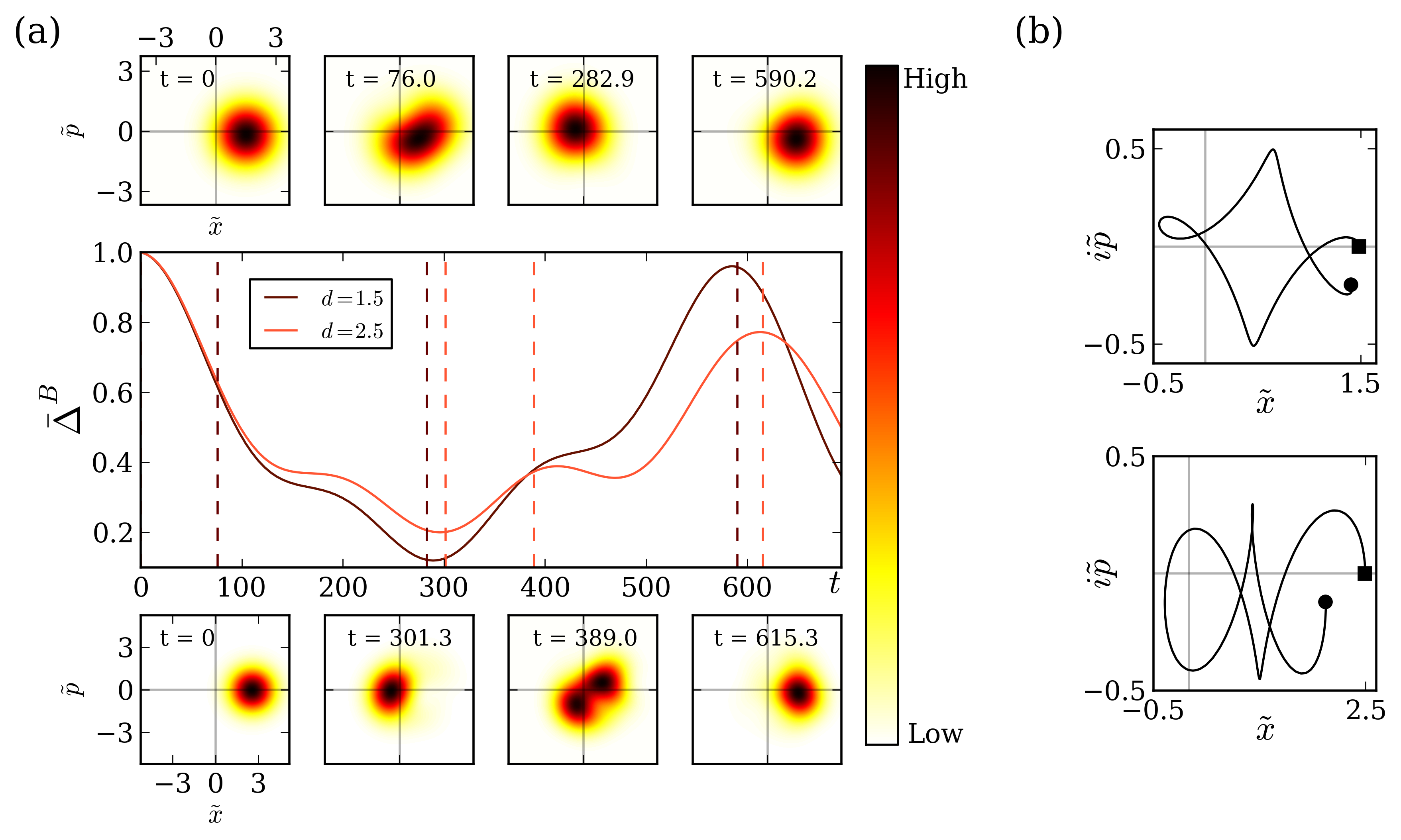
Figure 4: (a) Normalized excess energy $\bar{\Delta}^{B}(t)$ for $N_{A}=2$ and $d=1.5,2.5$. At characteristic points in time, $\tilde{Q}^{B}_{t}(z,z^{*})$ is shown (upper row: $d=1.5$, lower row: $d=2.5$). (b) $\bar{z}_{t}/\sqrt{2}$ trajectory for $d=1.5$ ($d=2.5$) until $t=590.2$ ($t=615.3$) in upper (lower) panel. The initial (final) value of $\bar{z}_{t}/\sqrt{2}$ is indicated by a square (circle). All quantities in HO units of $\hat{H}_{B}$.

As a matter of fact, $\tilde{Q}^{B}_{t}(z,z^{*})$ reflects the dissipative dynamics of the $B$ atom. The distance $\bar{r}_{t}$ of the mean value $\bar{z}_{t}$ of $\overline{\tilde{Q}^{B}_{t}}(z,z^{*})$ from the origin decreases (increases) with decreasing (increasing) energy of the $B$ atom (cf. fig. 4 (b)).

On the other hand, the shape of $\tilde{Q}^{B}_{t}(z,z^{*})$ provides us with information about the quantum state of $B$. In all our investigations for low excess energies, $\tilde{Q}^{B}_{t}(z,z^{*})$ resembles a Gaussian during most of the dynamics, undergoing a breathing into the $\varphi$- and $r$-directions with a relatively constant mean value $\bar{z}$ on the time-scale of a $B$ oscillation. Drastic shape changes are only observed during short time periods lasting a few $B$ oscillations and are accompanied with drifts of the phase $\bar{\varphi}_{t}$ of $\bar{z}_{t}$. During these time periods, $\tilde{Q}^{B}_{t}(z,z^{*})$ features a less symmetric shape, e.g. of a squeezed state as for $d=1.5$ at $t=76.0$. As can be inferred from fig. 4 (a), this short time period coincides with a rapid energy flux from $B$ to $A$. This suggests that the directed inter-species energy transfer is mediated through non-coherent $B$ states.

In our frame of reference, the time-dependence of $\bar{\varphi}_{t}$ is due to the collisional coupling to the environment. From the Husimi distribution and the $\bar{z}_{t}$ trajectory in fig. 4 (b), we infer that $\bar{z}$ accumulates a collisional phase shift. At $t=282.9$, i.e. when $\bar{\Delta}^{B}(t)$ is minimal, a phase shift of $\bar{\varphi}_{t}\approx\pi$ is observed for $d=1.5$. Remarkably, at $t=590.2$, the phase shift $\bar{\varphi}_{t}\approx 2\pi$ indicates that the initial state is almost fully recovered.

In the case of a displacement $d=2.5$, the excess energy $\varepsilon$ is almost three times larger than for $d=1.5$. In this case, our results are of lower accuracy (cf. B). First of all, we note that the extrema of $\bar{\Delta}^{B}(t)$ are less pronounced than for $d=1.5$ such that the recovery of the initial energy is less incomplete. Ultimately, one finding is similar for the higher displacement: most of the time, $\tilde{Q}^{B}_{t}(z,z^{*})$ roughly resembles a Gaussian. Again, only within a short time period the shape changes drastically. $\tilde{Q}^{B}_{t}(z,z^{*})$ then differs significantly from a Gaussian, as observed for $d=2.5$ at $t=389.0$.

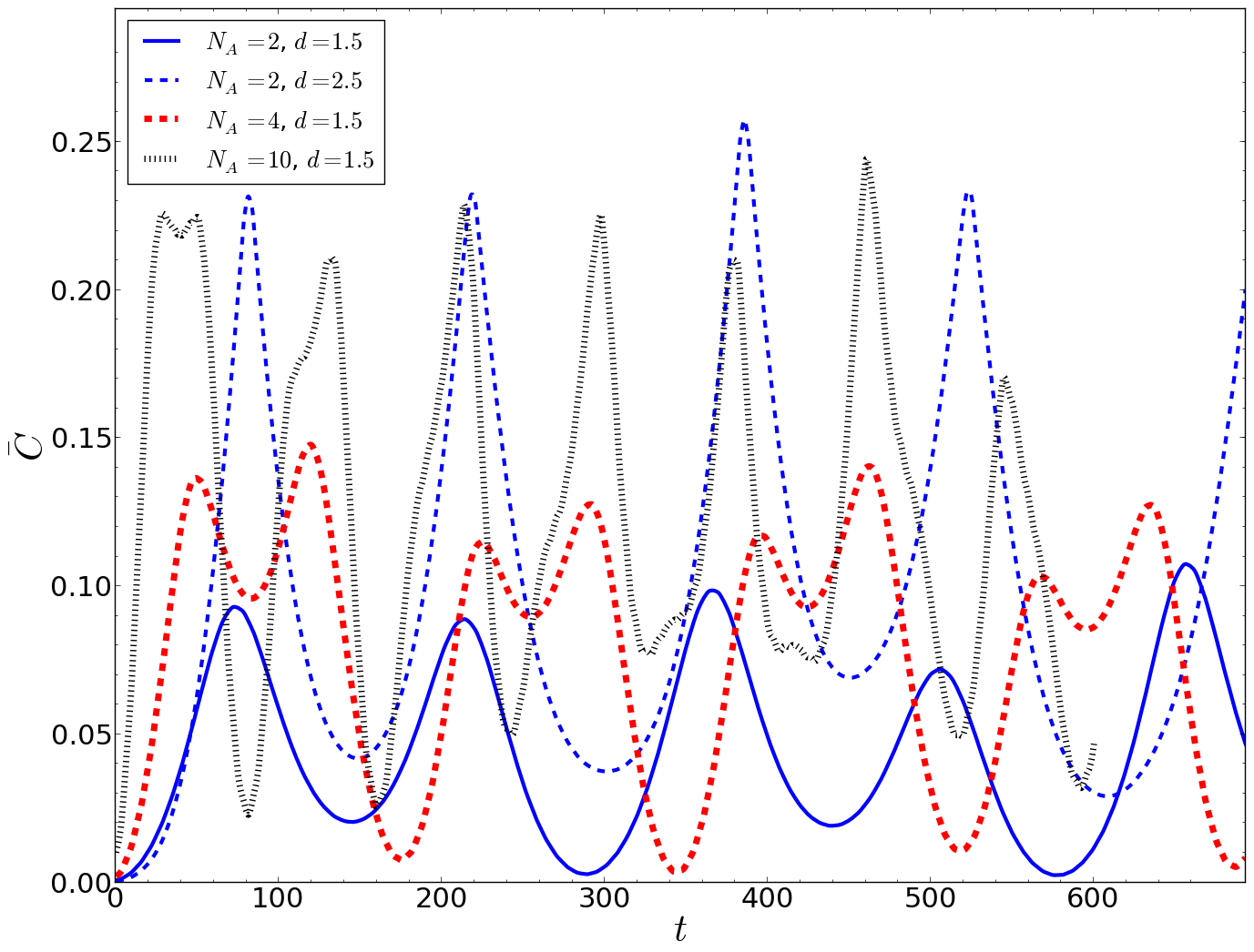
Figure 5: The coherence measure $\bar{C}(t)$ for $N_{A}=2$ (blue, solid line), $N_{A}=4$ (red, dashed) and $N_{A}=10$ (black, dotted) with $d=1.5$. Blue dashed line: $N_{A}=2$ with $d=2.5$. All quantities shown in HO units of $\hat{H}_{B}$.

In order to quantify the coherence of the $B$ quantum state (see fig. 5), we employ an operator norm to measure the distance of $\hat{\rho}^{B}_{t}$ from its closest coherent state:

$$C_{t}=\frac{1}{2}\inf_{z}\tr([\hat{\rho}^{B}_{t}-|z\rangle\!\langle z|]^{2})=\frac{1}{2}\Big{[}1+\tr\big{(}[\hat{\rho}^{B}_{t}]^{2}\big{)}-2\pi\sup_{z}{Q}^{B}_{t}(z,z^{*})\Big{]}.$$ (11)

We note that $C_{t}\in[0,1)$ and $C_{t}=0$ if and only if $B$ is in a coherent state. Focusing firstly on $N_{A}=2$ and $d=1.5$, the implications drawn from the evolution of $\tilde{Q}^{B}_{t}(z,z^{*})$ persist as depicted in fig. 4: At instants of extremely imbalanced energy distribution among $A$ and $B$, $B$ is very close to a coherent state as indicated by $\bar{C}(t)\approx 0$ at $t\approx 289$ and $t\approx 584$. For $d=1.5$ and $N_{A}=2$, the local minima of $\bar{C}(t)$, e.g. at $t\approx 145$, approximately coincide with the periods of decelerated energy transfer. For larger $d$ and $N_{A}=2$, the initial coherence is less restored at instants of extremal excess energy imbalance and, in between, the state of $B$ deviates more strongly from a coherent one. The recovery of the coherence also becomes less complete and the maximum of $\bar{C}(t)$ increases as the size of the environment is increased while $d=1.5$ is kept fixed (cf. $N_{A}=4,10$). Moreover, as we will see in sect. 5.1, the coherence measure $C_{t}$ strongly resembles the time evolution of the inter-species correlations. This finding suggests that the temporal deviations from a coherent state are caused by $\hat{\rho}^{B}_{t}$ becoming mixed.

4.3 State characterization of the bosonic environment

In this section, we investigate how the initially condensed state of the finite bosonic environment evolves structurally, thereby finding oscillations of the $A$ species depletion, whose amplitude is suppressed when increasing $N_{A}$ while keeping $\varepsilon$ fixed. We stress that the term “condensed” is not used in the quantum-statistical sense but shall refer to situations when all $N_{A}$ bosons approximately occupy the same single-particle state. For this analysis, we employ the concept of natural orbitals (NOs) and natural populations (NPs) [49], which are defined as the eigenvectors and eigenvalues of the reduced density operator of a certain subsystem in general. The spectral decomposition of the reduced one-body density operators for the species, $\sigma=A,B$, in particular reads:

$$\hat{\rho}^{\sigma}_{t}=\sum_{i=1}^{m_{\sigma}}\lambda^{\sigma}_{i}(t)\,|\varphi^{\sigma}_{i}(t)\rangle\!\langle\varphi^{\sigma}_{i}(t)|,$$ (12)

where $m_{\sigma}$ denotes the number of considered time-dependent single-particle basis functions in the ML-MCTDHB method (cf. A). Due to our normalization of reduced density operators, the $\lambda^{\sigma}_{i}(t)\in[0,1]$ add up to unity. In the following, we label the NPs in a decreasing sequence $\lambda^{\sigma}_{i}(t)\geq\lambda^{\sigma}_{i+1}(t)$ if not stated otherwise.

For characterizing the state of the bosonic ensemble, we use the NP distribution corresponding to the density operator of a single $A$ boson $\hat{\rho}^{A}_{t}$: If $\lambda_{1}^{A}(t)\approx 1$, the bosonic ensemble is called condensed [50], whereas slight deviations from this case indicate quantum depletion. Since it is conceptually very difficult to relate the NP distribution $\lambda_{i}^{A}(t)$ to intra-species (and also inter-species) correlations, we may only regard the $\lambda_{i}^{A}(t)$ as a measure for how mixed the state of a single $A$ atom is.

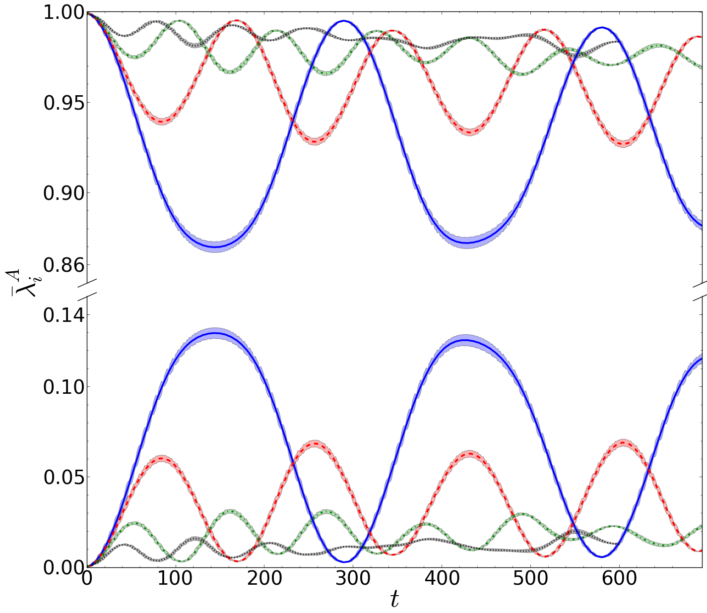
Figure 6: Dominant and second dominant NP of the reduced one-body density operator of a single $A$ boson for $N_{A}=2$ (blue, solid line), $N_{A}=4$ (red, dashed), $N_{A}=7$ (green, dashed dotted) and $N_{A}=10$ (black, dotted). The shaded areas indicate the standard deviation corresponding to the $\lambda^{A}_{i}(t)$ short-time dynamics, cf. (7). Other parameters: $\alpha=1$, $d=1.5$. All quantities shown in HO units of $\hat{H}_{B}$.

For $d=1.5$, only two NOs are actually contributing to $\hat{\rho}^{A}_{t}$ - the other NPs are smaller than $8.7\cdot 10^{-3}$. Therefore, we depict only the first two NPs for $N_{A}=2,4,7,10$ in fig. 6. Due to the weak intra-species interaction strength, the initial depletion of the bosonic ensembles is negligibly small, $1-\lambda_{1}^{A}(0)<10^{-3}$. One clearly observes that the $A$ species becomes dynamically depleted and afterwards approximately condenses again in an oscillatory manner. The instants of minimal depletion coincide with the instants of maximal excess energy imbalance between the subsystems for $N_{A}=2$. Therefore, the two bosons behave collectively in the sense that both approximately occupy the same single-particle state not only during time periods when the $A$ species is effectively in the ground state of $\hat{H}_{A}$ but also when $1-\bar{\Delta}^{B}(t)$ becomes maximal. For larger $N_{A}$, the depletion minima turn out to be less strictly synchronized with the $\bar{\Delta}^{B}(t)$ extrema. We will encounter the same finding for the strength of inter-species correlations in sect. 5.1 and discuss the details there.

Strikingly, the maximal depletion is significantly decreasing with increasing $N_{A}$. In C, we show that when neglecting the intra-species interaction the higher order NPs are bounded by $\lambda^{A}_{i}(t)\lesssim d^{2}/(2N_{A})$, $i\geq 2$, for sufficiently large $N_{A}$, which is a consequence of the gapped excitation spectrum, the extensitivity of the energy of the $A$ species and the fixed excess energy $d^{2}/2$. Although this line of argument neglects intra-species interactions, which will become important for larger $N_{A}$, the numerically obtained depletions lie well below the above bound.

5 Correlation analysis of the subsystems

As we consider a bipartite splitting of our total system, a Schmidt decomposition $|\Psi_{t}\rangle=\sum_{i}\sqrt{\lambda^{B}_{i}(t)}|\Phi^{A}_{i}(t)\rangle|\varphi^{B}_{i}(t)\rangle$ shows that the eigenvalue distributions of $\hat{\rho}^{B}_{t}$ and the reduced density operator for the $A$ species,

$$\hat{\eta}^{A}_{t}=\tr_{B}|\Psi_{t}\rangle\!\langle\Psi_{t}|=\sum_{i=1}^{m_{B}}\lambda^{B}_{i}(t)\,|\Phi^{A}_{i}(t)\rangle\!\langle\Phi^{A}_{i}(t)|,$$ (13)

coincide. Here, we study both the emergence of inter-species correlations on a short time-scale and their long-time dynamics in sect. 5.1. In particular, we show analytically that these correlations essentially vanish whenever the excess energy $\varepsilon^{\sigma}_{t}$ of one species $\sigma=A,B$ is much lower than the excitation gap of $\hat{H}_{\sigma}$. In sect. 5.2, we then unravel the energy transfer between the species by inspecting the energy stored in the respective NOs $|\Phi^{A}_{i}(t)\rangle$, $|\varphi^{B}_{i}(t)\rangle$ of the subsystems. Thereby, we identify incoherent energy transfer processes, which are related to inter-species correlations and shown to accelerate the early energy donation of the $B$ atom to the $A$ species.

5.1 Inter-species correlations

The NPs $\lambda_{i}^{B}(t)$ are directly connected to inter-subsystem correlations: Since the $B$ species consists of a single atom being distinguishable from the $A$ atoms, and since the bipartite system always stays in a pure state, the initial pure state of the $B$ atom characterized by $\lambda_{1}^{B}(0)=1$ can only become mixed if inter-species correlations are present. Deviations from $\lambda_{1}^{B}(t)=1$ indicate entanglement between the single atom and the species of $A$ bosons. In order to quantify these inter-subsystem correlations, we employ the von Neumann entanglement entropy:

$$S_{\rm vN}(t)=-{\rm tr}\left(\hat{\rho}^{B}_{t}\,\log\hat{\rho}^{B}_{t}\right)=-\sum_{i=1}^{m_{B}}\lambda_{i}^{B}(t)\,\log\lambda_{i}^{B}(t),$$ (14)

which vanishes if and only if inter-species correlations are absent, i.e. $|\Psi_{t}\rangle=|\Phi^{A}_{1}(t)\rangle|\varphi^{B}_{1}(t)\rangle$.

For all considered $N_{A}$, the von Neumann entropy of both the ground state of $\hat{H}$ and our initial condition $|\Psi_{0}\rangle$ with $d=1.5$ does not exceed $3.5\cdot 10^{-3}$, which is negligible compared to the dynamically attained values depicted in fig. 7. Thus, we may conclude that (i) the spatio-temporarily localized coupling requires a certain amount of excess energy for the subsystems to entangle and (ii) inter-species correlations are dynamically established via interferences involving excited states.

In fig. 7 (a), we present the short-time dynamics of the $S_{\rm vN}(t)$ for $N_{A}=2$. The entanglement between the single $B$ atom and the two $A$ bosons is built up in a step-wise manner with each collision. Since the local maxima of $S_{\rm vN}(t)$ are delayed w.r.t. the corresponding maxima of $\langle\hat{H}_{AB}\rangle_{t}$, we conclude that a finite interaction time is required in order to enhance correlations. After a few $B$ oscillations, the effective interaction time is increased since (i) dissipation moves the left turning point of the $B$ atom from $x=-d<-R$ towards the centre of the $A$ species at $x=-R$ and (ii) the $A$ / $B$ species density oscillations become synchronized (cf. fig. 3). As a consequence, the overall slope of $S_{\rm vN}(t)$ increases during the first few $B$ oscillations. We note that such a step-wise emergence of correlations has been reported also in [28] for two atoms colliding in a single harmonic trap.

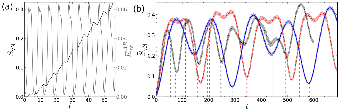
Figure 7: (a) Short-time evolution of the von Neumann entanglement entropy $S_{\rm vN}(t)$ (black line, left ordinate) and inter-species interaction energy $E^{AB}_{\rm int}(t)=\langle\hat{H}_{AB}\rangle_{t}$ (grey, right ordinate) for $N_{A}=2$ (data not time-averaged). (b) Long-time evolution of $\bar{S}_{\rm vN}(t)$ for $N_{A}=2$ (blue solid line), $N_{A}=4$ (red, dashed) and $N_{A}=10$ (black, dotted). The vertical dashed (dotted) lines in the respective colour indicate the instants of local $\bar{\Delta}^{B}(t)$ minima (maxima) read off fig. 2 (for clarity, we only show these reference lines until $t=320$ for $N_{A}=10$). The shaded areas indicate the standard deviation of $S_{\rm vN}(t)$ from $\bar{S}_{\rm vN}(t)$. Other parameters for both subplots: $\alpha=1$, $d=1.5$. All quantities shown in HO units of $\hat{H}_{B}$.

Concerning the long-time dynamics, we first focus on the $N_{A}=2$ case in fig. 7 (b). The correlation increase continues until a maximum at $t\approx 78$, which is followed by a minimum around $t\approx 144$ of modest depth, a further maximum at $t\approx 210$ and a deep minimum at $t\approx 288$. This alternating sequence of maxima and minima is repeated thereafter. In passing, we note that to some extent similar entropy oscillations with a long period comprising many collisions have been reported for two atoms in a single harmonic trap interacting with repulsive and attractive contact interaction in [28] and [32], respectively. As indicated by the vertical lines, the deep minima of $\bar{S}_{\rm vN}(t)$ at $t\approx 288$ and $t\approx 580$ coincide very well with instants of both a maximally imbalanced excess energy distribution among the species (cf. fig. 2) and minimal $A$ species depletion (cf. fig. 6).

This intimate relationship between maximal excess energy imbalance and absence of correlations can be understood analytically by expressing $\langle\hat{H}_{B}\rangle_{t}$ as a function(al) of the NPs and NOs,

$$\langle\hat{H}_{B}\rangle_{t}=\sum_{i=1}^{m_{B}}\lambda_{i}^{B}(t)\,\langle\varphi^{B}_{i}(t)|\hat{H}_{B}|\varphi^{B}_{i}(t)\rangle,$$ (15)

and identifying $\Sigma^{B}_{i}(t)=\langle\varphi^{B}_{i}(t)|\hat{H}_{B}|\varphi^{B}_{i}(t)\rangle$ with the energy content of the $i$-th NO. In D, we show that $\varepsilon^{B}_{t}$ being much smaller than the excitation gap $(E^{B}_{1}-E^{B}_{0})$ implies $\lambda_{i}^{B}(t)\ll 1$ for $i>1$. At those instants, the presence of an excitation gap prevents correlations between the subsystems due to a lack of orthonormal states $|\varphi^{B}_{i}(t)\rangle$, $i>1$, with excess energy $\varepsilon^{B}_{i}(t)=\Sigma^{B}_{i}(t)-E^{B}_{0}$ being of $\mathcal{O}(\varepsilon^{B}_{t})$. The same line of arguments analogously holds also for instants when $\varepsilon^{A}_{t}$ is much smaller than the excitation gap of $\hat{H}_{A}$. In between instants of maximal excess energy imbalance, more states are energetically accessible such that inter-species correlations can be established. Increasing $N_{A}$ while keeping $d=1.5$ alters the $\bar{S}_{\rm vN}(t)$ dynamics in the following way:

(i) Inter-species correlations initially emerge faster because binary collisions become more likely within a $B$ oscillation (cf. $N_{A}=2,4,10$ curves for $t<35$).

(ii) The depth of shallower minima decreases (cf. the $N_{A}=4$ curve at e.g. $t\approx 83$) such that neighbouring pairs of local maxima (cf. the $N_{A}=4$ curve at e.g. $t\approx 60$ and $t\approx 107$) degenerate to a single maximum for $N_{A}>4$ (all entropy minima for e.g. $N_{A}=10$ correspond to the deep minima observed for smaller $N_{A}$).

(iii) We find the coincidence of the deep entropy minima with extrema in the excess energy imbalance $\bar{\Delta}^{B}(t)$ to be less established. For e.g. $N_{A}=4$, the first deep $\bar{S}_{\rm vN}(t)$ minimum at $t\approx 169$ is attained before the first $\bar{\Delta}^{B}(t)$ minimum at $t\approx 195$. Since the overall energy donation of the $B$ atom is less efficient for $N_{A}=4$ (compared to $N_{A}=2$), $\bar{S}_{\rm vN}(t)$ is not forced to attain a deep minimum at the first minimum of $\bar{\Delta}^{B}(t)$ in the sense of the above analytical line of argument. For $N_{A}=10$, $\bar{\Delta}^{B}(t)$ essentially fluctuates around $0.65$ for $t>60$ such that the excitation gaps do not impose any restrictions on $\bar{S}_{\rm vN}(t)$.

(iv) The minimal value of $\bar{S}_{\rm vN}(t)$ for $t>0$ increases, which goes hand in hand with the energy donation of the $B$ atom becoming less efficient and the energy transfer cycle becoming less complete.

(v) The maximal values of $\bar{S}_{\rm vN}(t)$ are all comparable for $N_{A}\leq 10$. We note that the persistence of inter-species correlations when increasing $N_{A}$ does not contradict the fact that the $A$ species becomes simultaneously more condensed (cf. sect. 4.3), which can be easily seen by a minimal example provided in E.

5.2 Energy distribution among natural orbitals and incoherent transfer processes

In this section, we unravel the impact of the previously identified inter-species correlations on the energy transfer and identify incoherent transfer processes. For this purpose, we will evaluate the contribution of $\Sigma^{B}_{i}(t)$ to $\langle\hat{H}_{B}\rangle_{t}$ and complement this energy decomposition by analysing how the energy of the $A$ species is distributed among the $A$ species NOs $|\Phi^{A}_{i}(t)\rangle$:

$$\langle\hat{H}_{A}\rangle_{t}=\sum_{i=1}^{m_{B}}\lambda^{B}_{i}(t)\,\Sigma^{A}_{i}(t).$$ (16)

Here, we have introduced the energy content of the $i$-th $A$ species NO: $\Sigma^{A}_{i}(t)=\langle\Phi^{A}_{i}(t)|\hat{H}_{A}|\Phi^{A}_{i}(t)\rangle$. We remark that the presence of intra-species interaction prevents us from expressing $\langle\hat{H}_{A}\rangle_{t}$ as a function(al) of the NPs and NOs of $\hat{\rho}^{A}_{t}$ in a similar fashion as in (15). The highly challenging task of diagonalizing the reduced density operator $\hat{\eta}^{A}_{t}$ of the whole $A$ species for obtaining the $N_{A}$-body states $|\Phi^{A}_{i}(t)\rangle$, however, can be faced efficiently with the ML-MCTDHB method due to its beneficial representation of the many-body wave function (cf. A). We note that the NO energy contents $\Sigma^{A/B}_{i}(t)$ constitute system-immanent, basis-independent quantities as they result from the diagonalization of reduced density operators.

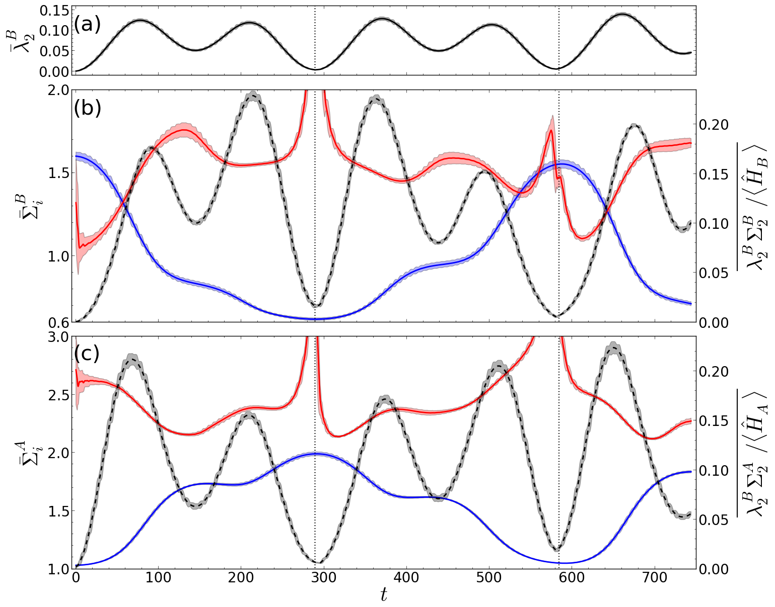
Figure 8: (a) Second dominant NP of $\hat{\rho}^{B}_{t}$. (b)/(c) NO energy content $\bar{\Sigma}^{\sigma}_{i}(t)$ of the first ($i=1$, blue solid line) and second ($i=2$, red) NO of species $\sigma=A/B$ (left ordinate). Black dashed line: Weighted contribution of the second dominant NO to the respective intra-species energy (right ordinate). The vertical dotted lines at $t\approx 289$ ($t\approx 584$) indicate the instants of minimal (maximal) $\bar{\Delta}^{B}(t)$. The shaded areas indicate the standard deviation from the respective locally time-averaged quantity. System parameters: $N_{A}=2$, $\alpha=1$, $d=1.5$. All quantities shown in HO units of $\hat{H}_{B}$.

For the considered displacement $d=1.5$ and all considered $N_{A}$, we find that only two NOs contribute to $\hat{\rho}^{B}_{t}$ and $\hat{\eta}^{A}_{t}$ ($\lambda^{B}_{i}\lesssim 7.6\cdot 10^{-3}$ for $i>2$) so that we only analyse their energy contents in fig. 8. Larger displacements generically result in more populated NOs and thus a much more involved dynamics, whose analysis goes beyond the scope of this work. In fig. 8, we bring the evolution of the second NP $\bar{\lambda}^{B}_{2}(t)$ face to face with the energy contents of the dominant and the second dominant NOs $\bar{\Sigma}^{A/B}_{i}(t)$, $i=1,2$, for the case of $N_{A}=2$ bosons. The NP of the dominant NO can be inferred from $\bar{\lambda}^{B}_{1}(t)\approx 1-\bar{\lambda}^{B}_{2}(t)$. Since $\bar{\Sigma}^{\sigma}_{i}(t)$ does not contain information about how much energy of the $\sigma$ species is actually stored in the corresponding NO, we moreover quantify the contribution of the second NO to the subsystem energy in terms of the ratio $\overline{\lambda^{B}_{2}\Sigma^{\sigma}_{2}/\langle\hat{H}_{\sigma}\rangle}(t)$.

We clearly observe that the energy content of the dominant NO, $\bar{\Sigma}^{A/B}_{1}(t)$, qualitatively resembles the subsystem energy $\bar{H}_{A/B}(t)$ evolution (cf. fig. 2). However, at time periods when inter-species correlations are present, i.e. when $\bar{\lambda}^{B}_{2}(t)\gtrsim 3\cdot 10^{-2}$, a significant fraction of the subsystem energy is stored in the respective second dominant NO. This fraction can become as large as $23\%$. Since essentially all subsystem energy is stored in the respective dominant NO whenever $\bar{\Delta}^{B}(t)$ is extremal (cf. at $t\approx 289$ and $t\approx 584$) and since the evolution of $\overline{\lambda^{B}_{2}\Sigma^{A}_{2}/\langle\hat{H}_{A}\rangle}(t)$ appears to be synchronized with the dynamics of $\overline{\lambda^{B}_{2}\Sigma^{B}_{2}/\langle\hat{H}_{B}\rangle}(t)$, we conclude that the energy transfer is mediated via incoherent processes in the following sense: Rather than keeping all its instantaneous energy in the dominant NO, the $B$ atom shuffles energy from the dominant to the second NO and back while donating (accepting) energy to (from) the $A$ species. The $A$ species, in turn, accepts (donates) energy from (to) the $B$ atom while shuffling energy from the dominant to the second NO and back. As predicted by the analytical line of argument in D, one can furthermore witness how the intra-species excitation gap of the $\sigma$ species makes the second NO to energetically separate drastically from the dominant one when $\varepsilon^{\sigma}_{t}$ becomes too small (cf. $\bar{\Sigma}^{B}_{2}(t)$ at $t\approx 289$ and $\bar{\Sigma}^{A}_{2}(t)$ at $t\approx 584$). Finally, we observe that $\bar{\Sigma}^{A/B}_{2}(t)>\bar{\Sigma}^{A/B}_{1}(t)$ holds most of the time. Consequently, if the $B$ atom has been detected in the NO of lower (higher) energy, the $A$ species is found almost certainly in the NO of lower (higher) energy and vice versa, according to the above Schmidt decomposition.

The above overall picture of the NO energy content evolution remains valid for all $N_{A}\leq 10$, while the relationship between the inter-species energy transfer and the distribution of the subsystem energies among the respective NOs becomes more involved for larger environments. Whereas $\overline{\lambda^{B}_{2}\Sigma^{A/B}_{2}/\langle\hat{H}_{A}\rangle}(t)$ remains synchronized with $\bar{S}_{\rm vN}(t)$ when going to larger $N_{A}$, the inter-species correlation dynamics becomes less strictly synchronized with the $\bar{\Delta}^{B}(t)$ evolution as discussed at the end of sect. 5.1 in detail. With increasing $N_{A}$, we moreover observe the tendency that each species temporarily stores a slightly more significant fraction of its energy also in the third and fourth dominant NO despite their quite low populations. We suspect that this increase in complexity might be related to the observed decay of the excess energy imbalance to a rather balanced distribution for $N_{A}=7,10$ (cf. fig. 2). Finally, we summarize peculiarities concerning $N_{A}=2$, which are diminished or absent for larger environment sizes: Firstly, the decelerated energy transfer around $t\approx 160$ coincides with a time period of significant contribution of the second NO to $\bar{H}_{B}(t)$ so that the incoherent processes can be made partially responsible for the delay. Secondly, pairs of subsequent $\overline{\lambda^{B}_{2}\Sigma^{A/B}_{2}/\langle\hat{H}_{A/B}\rangle}(t)$ maxima in between consecutive deep minima (e.g. at $t\approx 91$ and $t\approx 214$) are related to the observed pairs of local $\bar{S}_{\rm vN}(t)$ maxima and, thus, merge to a single maximum for larger $N_{A}$.

Finally, we analyse how the overall energy transfer is influenced by these incoherent energy transfer processes. The ML-MCTDHB method allows to manually switch off inter-species correlations in order to clarify their role for the dynamics (cf. A). By comparison, we have found for all considered $N_{A}$ that the presence of inter-species correlations accelerates the energy donation of the $B$ atom at first, i.e. for $t\lesssim 50$, which is plausible since more energy transfer channels are open. Whether the overall energy donation is accelerated, however, depends on $N_{A}$: For $N_{A}=2$, we observe an acceleration by a factor of two, while for $N_{A}=7$ no overall acceleration is found (plots not shown).

6 Excitations in Fock space and their correlations

Operating in the weak interaction regime, we naturally define intra-system excitations as occupations of excited single-particle eigenstates corresponding to the respective HO Hamiltonian. The joint probability for finding $(n_{0},n_{1},...)$ $A$ bosons in the respective HO eigenstates and the $B$ atom in its $j$-th HO eigenstate is given by:

$$P_{t}(n_{0},n_{1},...;j)=\left|\,\langle\Psi_{t}|\left(|n_{0},n_{1},...\rangle^{A}_{\rm HO}\otimes|u_{j}^{B}\rangle\right)\,\right|^{2}.$$ (17)

In this chapter, we firstly show that the actual long-time excitation dynamics takes place only in certain active subspaces being mutually decoupled (sect. 6.1). Secondly, the $A$ species excitations are shown to be governed by singlet and delayed doublet excitations (sect. 6.2). The findings of these two sections are explained by means of a tailored time-dependent perturbation theory. Finally, correlations between the intra-species excitations of $A$ and $B$ are shown to (dis-)favour certain energy transport channels depending, in general, on the direction of energy transfer (sect. 6.3).

6.1 Decoupled active subspaces

For a fixed total single-particle energy $E_{\rm SP}(k)=k+(N_{A}+1)/2$, $k\in\mathbb{N}_{0}$, we have evaluated the probability $P_{\rm SP}(k;t)$ to find the bipartite system in the subspace spanned by configurations $|n_{0},n_{1},...\rangle^{A}_{\rm HO}\otimes|u^{B}_{j}\rangle$ with total single-particle energy $E_{\rm SP}(k)$. So $P_{\rm SP}(k;t)$ is obtained by summing over all $P_{t}(n_{0},n_{1},...;j)$ with $j+\sum_{r\geq 1}r\,n_{r}=k$. In fig. 10 (a), we depict the probabilities $\bar{P}_{t}(n_{0},n_{1},...;j)$ for the configurations of total single-particle energy $E_{\rm SP}(1)$, $|N_{A},0,...\rangle^{A}_{\rm HO}\otimes|u^{B}_{1}\rangle$ and $|N_{A}-1,1,...\rangle^{A}_{\rm HO}\otimes|u^{B}_{0}\rangle$, for $N_{A}=4$, showing large amplitude oscillations while their sum $\bar{P}_{\rm SP}(1;t)$ (not shown) stays comparatively constant. In fact, we find $\bar{P}_{\rm SP}(k;t)$ to be approximately conserved for all considered $N_{A}$ and $d=1.5$. Thus, the actual energy transfer dynamics approximately happens solely within the various subspaces of fixed total single-particle energy $E_{\rm SP}(k)$, $k\geq 1$, while inter-subspace transitions are suppressed.

6.2 Intra-species excitations

The joint probability (17) describing the distribution of excitations in the total system defines the following two marginal distributions for the $A$ species and the single $B$ atom,

$$p^{A}_{t}(n_{0},n_{1},..) =\sum_{j}P_{t}(n_{0},n_{1},...;j)={}^{\;\;\;\,A}_{\;\rm HO}\langle n_{0},n_{1},...|\hat{\eta}^{A}_{t}|n_{0},n_{1},...\rangle^{A}_{\rm HO},$$ (18)

$$p^{B}_{t}(j) =\sum_{n_{0},n_{1},...}P_{t}(n_{0},n_{1},...;j)=\langle u^{B}_{j}|\hat{\rho}^{B}_{t}|u^{B}_{j}\rangle.$$ (19)

In order to classify the collisionally induced excitations in the environment, we inspect the probabilities for having no ($p_{t}^{A;0}$), a singlet ($p_{t}^{A;1}$) and a doublet excitation ($p_{t}^{A;2}$),

$$p_{t}^{A;0}=p^{A}_{t}(\vec{n}_{0}),\quad p_{t}^{A;1}=\sum_{i>0}p^{A}_{t}(\vec{n}_{0}^{i}),\quad p_{t}^{A;2}=\sum_{0<i\leq j}p^{A}_{t}(\vec{n}_{0}^{ij}),$$ (20)

where $\vec{n}_{0}=(N_{A},0,0,...)$ and $\vec{n}_{0}^{i}$ ($\vec{n}_{0}^{ij}$) refers to occupation number vectors with $N_{A}-1$ ($N_{A}-2$) atoms in the harmonic oscillator ground state and one (two) atom(s) in the $i$-th ($i$-th and $j$-th) excited state(s).

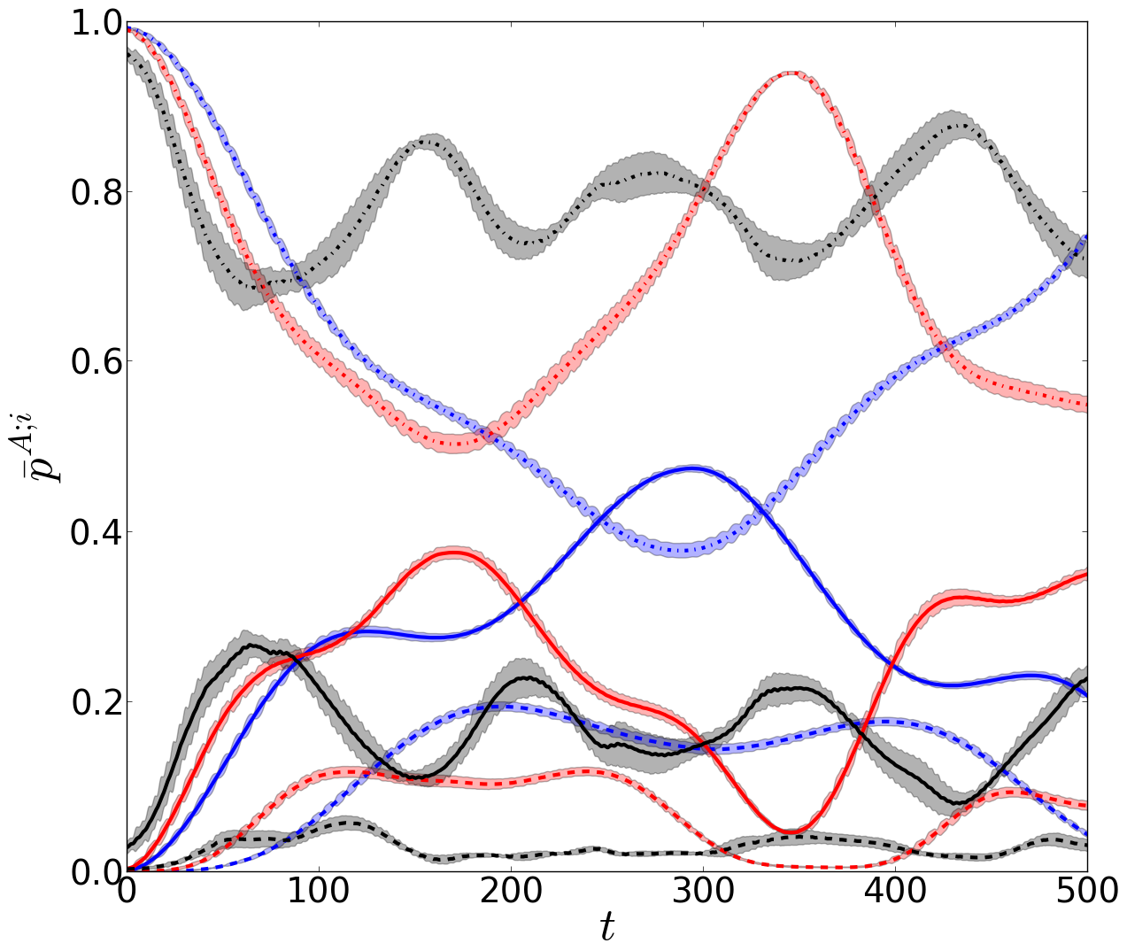
Figure 9: Probability $\bar{p}^{A;i}(t)$ for no ($i=0$, dashed dotted line), singlet ($i=1$, solid) and doublet ($i=2$, dashed) excitation(s) for $N_{A}=2$ (blue), $N_{A}=4$ (red) and $N_{A}=10$ (black). The shaded areas indicate the standard deviation from the respective locally time-averaged quantity. Other system parameters: $\alpha=1$, $d=1.5$. All quantities shown in HO units of $\hat{H}_{B}$.

In fig. 9, we compare these classes of $A$ species excitations for $N_{A}=2,4,10$: One can clearly see that the excitations attain a maximum (minimum) whenever $\bar{\Delta}^{B}(t)$ (cf. fig. 2) becomes minimal (maximal). Moreover, singlet excitations dominate over doublets (and also not shown higher order excitations), which occur only after a certain delay with respect to the appearance of singlets. As expected from energetical considerations, the singlet excitations involve dominantly the $|N_{A}-1,1,0,...\rangle^{A}_{\rm HO}$ configuration and second dominantly $|N_{A}-1,0,1,0...\rangle^{A}_{\rm HO}$, which can occur as likely as the dominant doublet contribution $|N_{A}-2,2,0,...\rangle^{A}_{\rm HO}$.

In sect. 3, the increasing number of collision partners has been argued to be responsible for the acceleration of the energy transfer with increasing $N_{A}$. Fig. 9 clearly shows this enhancement of excitation probability with increasing $N_{A}$ during the first few $B$ oscillations ($t\lesssim 80$). The larger $N_{A}$, the faster does the probability for singlet excitations increase. For $N_{A}=10$, this effect is less visible since the intra-species interaction results in a finite initial singlet probability. Concerning the long-time dynamics, we observe that the maximal singlet / doublet excitation probability reduces for larger environment sizes, which goes hand in hand with the energy donation to A becoming less efficient.

For obtaining analytical insights into the delayed doublet emergence and the decoupled active subspaces, we have applied a stroboscopic version of time-dependent perturbation theory to the simplest case of $g_{A}=0$. The total wave function $|\Psi_{r}\rangle$ after $r$ oscillations is propagated for one free oscillation period $T=2\pi$ with linear perturbation theory with respect to $\hat{H}_{AB}^{I}(t)$ (with $I$ denoting the interaction picture): $|\Psi^{I}_{r+1}\rangle=(\mathds{1}-i2\pi\bar{H}_{AB}^{I})|\Psi^{I}_{r}\rangle$, where the time-averaged coupling Hamiltonian reads

$$\bar{H}_{AB}^{I}=\frac{1}{2\pi}\int\limits_{2\pi r}^{2\pi(r+1)}{\rm d}\tau\,\hat{H}_{AB}^{I}(\tau)=g_{AB}\sum_{i,j,p,q}\delta_{i+j,q+p}\,v_{ijpq}\,{\hat{a}}^{\dagger}_{i}{\hat{a}}_{p}\otimes|u^{B}_{j}\rangle\!\langle u^{B}_{q}|.$$ (21)

The energy conservation enforced by the Kronecker $\delta_{i+j,q+p}$, being reminiscent of Fermi’s golden rule, is an immediate consequence of the equidistant single-particle spectra and $\alpha=1$. In order to avoid norm loss, we raise the above map to a unitary one, $|\Psi^{I}_{r+1}\rangle\approx\exp(-i\,2\pi\bar{H}_{AB}^{I})|\Psi^{I}_{r}\rangle$, which is equivalent to solving a temporally coarse-grained Schrödinger equation with the effective Hamiltonian $\bar{H}_{AB}^{I}$.

We have observed good agreement between full numerical simulations (with $g_{A}=0$) and the perturbation theory (plots not shown) concerning the observables $\bar{\Delta}^{B}(t)$ and $\bar{p}^{A;i}(t)$ during the first $18$ ($12$) collisions for $N_{A}=2$ ($N_{A}=7$). Yet the entanglement entropy turns out to be overestimated a bit earlier by the perturbative approach. Comparing our full numerical data for $g_{A}=0$ and $g_{A}=g_{AB}$, we find qualitative agreement during the first $r=10,...,20$ collisions such that the following insights from the perturbation theory should also apply in the presence of intra-species interaction. Firstly, one can easily show that $\bar{H}_{AB}^{I}$ commutes with the projector onto the subspace of configurations with fixed $E_{\rm SP}(k)$. Due to the detailed energy conservation in binary collisions, the temporally coarse-grained dynamics decouples subspaces of different total single-particle energy. Secondly, $\bar{H}_{AB}^{I}$ involves only one-body processes within the $A$ species. Therefore, doublets can only emerge after the second collision with - as second order processes w.r.t. to $\bar{H}_{AB}^{I}$ - smaller amplitude than singlets, which explains the suppression and delay of the doublet creation. It goes without saying that the perturbative approach breaks down after fewer collisions for larger $N_{A}$ since (i) the intra-species interaction becomes more relevant and (ii) the enhanced inter-species coupling $g_{AB}N_{A}$ leads to less separated time scales making a temporal coarse-graining questionable.

6.3 Correlations between intra-species excitations

Ultimately, we aim at unravelling correlations between excitations of the $B$ atom and the $A$ species. For this purpose, we introduce the following correlation measure:

$$g_{t}(n_{0},n_{1},...;j)=\frac{P_{t}(n_{0},n_{1},...;j)}{p^{A}_{t}(n_{0},n_{1},..)\,p^{B}_{t}(j)},$$ (22)

which is reminiscent of the diagonal of higher order coherence functions introduced by Glauber [51]. While $g_{t}(n_{0},n_{1},...;j)=1$ means that the intra-species excitations take place statistically independently, a value larger (smaller) than unity implies that the corresponding joint excitation event $(n_{0},n_{1},...;j)$ is measured with an enhanced (decreased) probability, i.e. (anti-)bunches.

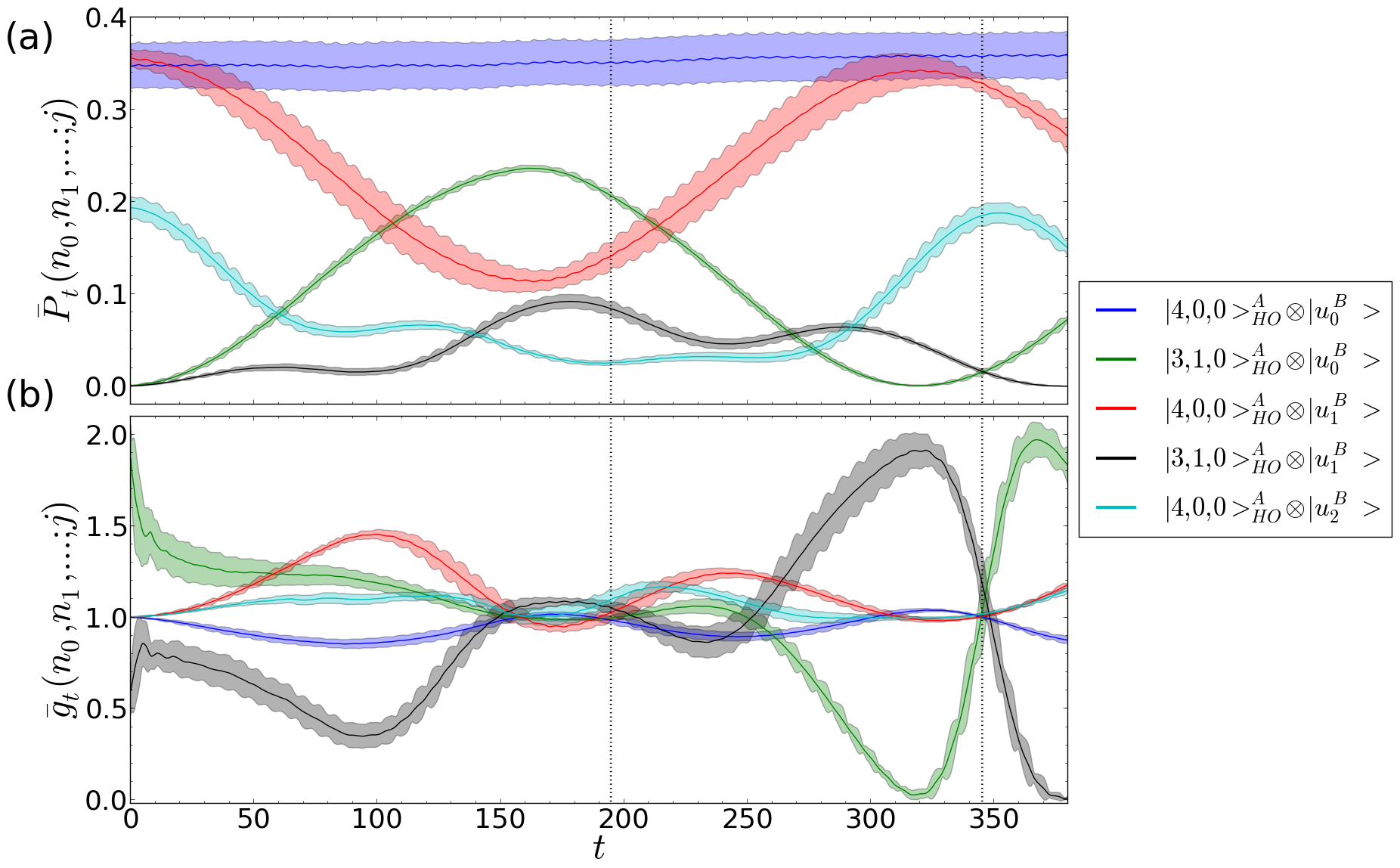
Figure 10: Joint probability $\bar{P}_{t}(n_{0},n_{1},...;j)$ (a) and correlation measure $\bar{g}_{t}(n_{0},n_{1},...;j)$ (b) for selected configurations of the bipartite system. The dashed vertical line at $t\approx 195$ ($t\approx 345$) indicates the instant of the $\bar{\Delta}^{B}(t)$ minimum (maximum) in the considered time-interval. The shaded areas indicate the standard deviation from the respective locally time-averaged quantity. Parameters: $N_{A}=4$, $\alpha=1$, $d=1.5$. All quantities shown in HO units of $\hat{H}_{B}$.

In fig. 10, we present the evolution of both the joint probability $\bar{P}_{t}(n_{0},n_{1},...;j)$ and the Fock space correlation measure $\bar{g}_{t}(n_{0},n_{1},...;j)$ for $N_{A}=4$ and selected configurations, which have a significant contribution to the total wave function. We emphasize that we do not intend to present a comprehensive overview over all energy transfer channels but rather concentrate on some important ones.

As expected, the considered excitations turn out to be uncorrelated whenever $\bar{S}_{\rm vN}(t)$ attains a deep minimum, which is partly related to extremal values of $\bar{\Delta}^{B}(t)$ as discussed in sect. 5.1. In between those instants, the subsystem configurations $|N_{A},0,...\rangle^{A}_{\rm HO}$, $|u^{B}_{0}\rangle$ are found slightly anti-bunched, while the occupation of the dynamically decoupled one-dimensional $E_{\rm SP}(0)$ subspace stays rather constant. In contrast to this, the configurations of the $E_{\rm SP}(1)$ subspace feature more involved correlations: Whereas the configurations $|N_{A},0,...\rangle^{A}_{\rm HO}$, $|u^{B}_{1}\rangle$ bunch, their counterparts $|N_{A}-1,1,0,...\rangle^{A}_{\rm HO}$, $|u^{B}_{0}\rangle$ are measured with enhanced (reduced) probability when the $B$ atom effectively donates (accepts) energy. The reverse statements hold for the configurations $|N_{A}-1,1,0,...\rangle^{A}_{\rm HO}$, $|u^{B}_{1}\rangle$ belonging to the $E_{\rm SP}(2)$ subspace. We conclude that, depending on the direction of the energy transfer, inter-species correlations stochastically favour or disfavour certain subsystem configurations and thereby energy transfer channels.

7 Conclusions and outlook

In this work, we have analysed the correlated energy transfer between a single atom and a finite, interacting bosonic environment mediated by a spatio-temporally localized coupling, focusing on an initial excess energy of the single atom just above the environment excitation gap. By ab-initio simulations of the whole system, we have shown that the energy transfer happens the faster the larger the number of environmental degrees of freedom $N_{A}$ is, which is explained classically by an increased number of collision partners and quantum-mechanically by a with $N_{A}$ increasing level splitting of the degenerate two first excited states of the uncoupled system. At the same time, the energy transfer between the subsystems becomes less complete when increasing $N_{A}$ so that the excess energy distribution oscillates around quite a balanced one for larger $N_{A}$, which might be regarded as a precursor of temporal relaxation induced by dephasing and has important consequences for inter-species correlations: While correlations are analytically shown to be suppressed whenever the excess energy distribution is maximally imbalanced, more balanced distributions allow for stronger correlations, which are dynamically established indeed. By inspecting the energy distribution among the natural orbitals of the $B$ atom as well as the whole $A$ species, incoherent transfer processes being intimately connected to inter-species correlations are unravelled. While donating (accepting) energy, each subsystem simultaneously shuffles a significant fraction of its energy into the second dominant natural orbital and back. These incoherent processes accelerate the early energy donation of the $B$ atom and might be experimentally detectable by correlating the outcomes of single shot energy measurements upon both subsystems. Moreover, by analysing correlations between subsystem excitations, we show that inter-species correlation (dis-)favour certain energy transfer channels depending on the instantaneous direction of transfer.

The correlated energy transfer dynamics manifests itself in the subsystem dynamics as follows: The $B$ atoms experiences a temporal loss of coherence in terms of short time periods during which the Husimi function undergoes significant shape changes. These deviations from a coherent state are more pronounced for larger $N_{A}$. The bosonic environment features depletion oscillations with a maximal depletion decreasing faster with increasing $N_{A}$ than its upper, energetically allowed bound $\propto 1/N_{A}$, which is derived for negligible intra-species interaction. In the considered low-excess energy regime, the excitations of the environment induced by the coupling to the $B$ atom mainly consist of singlet and delayed doublet excitations, whose delay is explained by a temporally coarse-grained Schrödinger equation.

To round off this work, we have made a proposal for an experimental realization of this open quantum system problem based on a combination of an optical dipole trap with a magnetic field gradient, which allows for a species-selective trapping of selected ⁸⁷Rb hyperfine states.

As an outlook, our work on systems with spatio-temporally localized couplings allows various interesting extensions: (i) Having understood the low-excess energy regime, a natural step consists in a careful increase of the excess energy in order to systematically open more and more energy transfer channels. (ii) It is important to address the questions whether the excess energy distribution among the subsystems temporally relaxes due to dephasing and whether inter-species correlations are persistent when significantly increasing $N_{A}$ to values $\mathcal{O}(100)$. However, such investigations will require to either separate the traps further or switch off / rescale the intra-species interaction strength in order to keep the initial inter-species overlap vanishing. (iii) The demonstrated tunability of the inter-species coupling matrix elements (5) in terms of the trap separation $R$ should be exploited to control the correlated energy transfer.

Achnowledgements

The authors would like to thank Oriol Vendrell, Hans-Dieter Meyer, Walter Strunz, Lushuai Cao and Antonio Negretti for inspiring discussions, Christof Weitenberg for valuable support concerning the experimental realizability of this system as well as Maxim Efremov for his expertise in phase-space analysis. S.K. acknowledges a scholarship of the Studienstiftung des deutschen Volkes and P.S. acknowledges funding by the Deutsche Forschungsgemeinschaft in the framework of the SFB 925 “Light induced dynamics and control of correlated quantum systems”.

Appendix A ML-MCTDHB method

Rather than considering the reduced dynamics for the single atom in terms of some effective master equation [6], we simulate here the correlated quantum dynamics of the total system by means of the recently developed ab-initio ML-MCTDHB method [37, 38]. Our method is based on three key ideas: (i) The total many-body wave function is expanded with respect to a time-dependent, optimally with the system co-moving many-body basis, which allows to obtain converged results with a significantly reduced number of basis states compared to expansions relying on a time-independent basis. (ii) The symmetry of the bosonic species is explicitly employed. (iii) The multi-layer ansatz for the total wave function is based on a coarse-graining cascade, which enables to adapt the ansatz to intra- and inter-species correlations and makes ML-MCTDHB to be a highly flexible, versatile tool for simulating the full dynamics of bipartite systems. Thereby, ML-MCTDHB incorporates both the coarse-graining concept of the Multi-Layer Multi-Configuration Time-Dependent Hartree Method [52, 53, 54] for distinguishable degrees of freedom and the explicit consideration of the particle exchange symmetry in the Multi-Configuration Time-Dependent Hartree Method for Bosons [55, 56] (cf. also [57] in this context). Compared to the direct extension of the latter method to mixtures [58], ML-MCTDHB can approach larger system sizes because of its adaptability to system-specific inter-species correlations.

Here, we summarize the ML-MCTDHB ansatz concretised for a binary bosonic mixture with particle numbers $N_{A}$ and $N_{B}$. Firstly, we assign $m_{\sigma}$ time-dependent single-particle basis functions $|\phi^{\sigma}_{i}(t)\rangle$, $i=1,...,m_{\sigma}$ to the species $\sigma=A,B$. These single-particle basis functions are then raised to a time-dependent $N_{\sigma}$-body basis by constructing bosonic number states $|n_{1},...n_{m_{\sigma}}\rangle_{t}^{\sigma}$ describing a fully symmetrized Hartree product with $n_{i}$ bosons of the $\sigma$ species occupying the state $|\phi^{\sigma}_{i}(t)\rangle$. Instead of considering all $(N_{\sigma}+m_{\sigma}-1)!/[N_{\sigma}!(m_{\sigma}-1)!]$ number state configurations on an equal footing, we consider only a reduced number of $M$ time-dependent species basis functions:

$$|\psi^{\sigma}_{j}(t)\rangle=\sum_{n_{1},...,n_{m_{\sigma}}|N_{\sigma}}C^{\sigma}_{j;n_{1},...,n_{m_{\sigma}}}(t)|n_{1},...n_{m_{\sigma}}\rangle_{t}^{\sigma},\quad$$ (23)

where $j=1,...,M$ and “$...|N_{\sigma}$” indicates that all occupation numbers must add up to $N_{\sigma}$. These “coarse-grained” species basis functions are finally used in order to expand the total wave function of the binary mixture:

$$|\Psi_{t}\rangle=\sum_{i_{A},i_{B}=1}^{M}A_{i_{A}i_{B}}(t)|\psi^{A}_{i_{A}}(t)\rangle\otimes|\psi^{B}_{i_{B}}(t)\rangle.$$ (24)

Having specified the ML-MCTDHB wave function ansatz, one employs a variational principle such as the Dirac-Frenkel [59, 60] or equivalently the McLachlan variational principle [61] for deriving the equations of motion both for the expansion coefficients $A_{i_{A}i_{B}}$ and the basis functions on the species layer, i.e. $C^{\sigma}_{j;n_{1},...,n_{m_{\sigma}}}$, as well as on the particle layer, i.e. $|\phi^{\sigma}_{i}\rangle$. Relying on a variational principle, these equations of motion ensure that the basis states move in a variationally optimally way so that at each instant in time one obtains an optimal representation of the total wave function for given numbers of species basis functions $M$ and single-particle basis function $m_{\sigma}$. The resulting set of coupled ordinary differential equations and non-linear partial differential equations, however, is too cumbersome to be discussed here and we refer to [37, 38] for the details. We note that the ML-MCTDHB method also allows for calculating low lying excited states by means of the improved relaxation algorithm [38, 62].

One key feature of the ML-MCTDHB ansatz lies in its flexibility (iii): It covers both the mean-field limit $M=m_{\sigma}=1$ and the numerical exact limit. The latter is achieved by considering as many single-particle particle basis functions as one employs time-independent basis states, e.g. grid points, in order to represent them and choosing $M={(N_{\sigma}+m_{\sigma}-1)!/[N_{\sigma}!(m_{\sigma}-1)!]}$. Moreover, in the presence of quite some intra-species but weak inter-species correlations, as it is often the case for system-environment problems, one might get converged results with $M$ being much smaller than ${(N_{\sigma}+m_{\sigma}-1)!/[N_{\sigma}!(m_{\sigma}-1)!]}$. In our particular situation with $N_{B}=1$, one has to choose $m_{B}=M$. So we have to ensure convergence with respect to numbers of grid points $n$ and time-dependent basis functions, i.e. $m_{A}$ and $M$. By setting the number of time-dependent optimized species layer basis functions $M=1$ while still bringing the simulation to convergence with respect to the number $m_{A}$ of time-dependent optimized $A$ boson single-particle basis functions, the ML-MCTDHB equations of motion give a variationally optimized solution for the many-body problem under the constraint of vanishing inter-species correlations, which can illuminate the role of inter-species correlations as discussed in sect. 5.2.

Appendix B Initial state preparation and convergence

In order to prepare our initial state, we first shift the harmonic trap for the single atom to the right by replacing $(\hat{x}^{B})^{2}/2$ by $(\hat{x}^{B}-d)^{2}/2$ in $\hat{H}_{B}$ and propagate an initial guess for (24) with the ML-MCTDHB equations of motion in imaginary time. Thereby, we relax the binary mixture to its many-body ground state. Due to the almost vanishingly small spatial overlap of the two species, the result of this procedure is a many-body wave function factorizing to good approximation into the ground state of $N_{A}$ interacting bosons in their harmonic trap and the single atom being in the coherent state $|z=d/\sqrt{2}\rangle$. Afterwards, we propagate this state with the unshifted Hamiltonian (1).

For representing the time-dependent single-particle basis functions, we employ a harmonic oscillator discrete variable representation [63, 64] with $n=401$ grid points. Concerning the size of the time-dependent basis, we ensured convergence by checking that incrementing $m_{A}$ or $M$ does at most slightly quantitatively affect physical observables such as energy and the natural populations on the species and particle layers. For our purposes, $m_{A}=3$ and $M=4$ turned out to lead to convergence for $N_{A}<10$ and $d=1.5$. For $N_{A}=10$, a $(m,M)=(3,3)$ simulation agree well with a $(3,4)$ run up to $t\sim 200$. Afterwards, the natural populations of the $(3,4)$ simulation still indicate convergence, yet an explicit convergence check for such long-time propagations by further increasing $m$ and $M$ is computationally prohibitive. Due to an decrease of the system time-scale $T_{\rm cycle}$ with $N_{A}$, it is very natural that high precision results until $t=700$ are much harder to obtain for $N_{A}=10$ compared to smaller boson numbers and so we have to work with variationally optimal results of somewhat lower accuracy. Similarly, simulations with larger excess energies are more demanding: For $N_{A}=2$ and $d=2.5$, we have checked the plotted $(3,4)$ results against $(5,5)$ simulations, indicating that the accuracy is somewhat lower compared to the case $d=1.5$ but sufficiently high for the considered observables.

Appendix C Bound on the $A$ species depletion

Neglecting the intra-species interaction, we show here that the depletion of the $A$ species vanishes as $1/N_{A}$ in the large $N_{A}$ limit as a consequence of the fixed excess energy and $\hat{H}_{A}$ featuring a gapped excitation spectrum. Setting $g_{A}=0$ and assuming the initial inter-species interaction energy to be negligible $\langle\hat{H}_{AB}\rangle_{0}\ll\langle\hat{H}\rangle_{0}$ (which is the case to a very good approximation in fact), energy conservation implies:

$$N_{A}E^{A}_{0}+E^{B}_{0}+\varepsilon\approx\langle\hat{H}_{A}\rangle_{t}+\langle\hat{H}_{B}\rangle_{t}+\langle\hat{H}_{AB}\rangle_{t}\geq\langle\hat{H}_{A}\rangle_{t}+E^{B}_{0},$$

given the excess energy $\varepsilon=d^{2}/2$. Since $\hat{H}_{A}$ contains only the single-particle Hamiltonians $\hat{h}^{A}_{i}={[({\hat{p}^{A}_{i}})^{2}+(\hat{x}^{A}_{i}+R)^{2}]/2}$ by assumption, we may express $\langle\hat{H}_{A}\rangle(t)$ as a function(al) of the $\hat{\rho}^{A}_{t}$ NPs / NOs sorted in increasing sequence with respect to their instantaneous excess energy $\tilde{\varepsilon}^{A}_{i}(t)=\langle\tilde{\varphi}^{A}_{i}(t)|\hat{h}^{A}_{1}|\tilde{\varphi}^{A}_{i}(t)\rangle-E^{A}_{0}$ being indicated by a tilde and obtain:

$$\tilde{\varepsilon}^{A}_{1}(t)+\sum_{i=2}^{m_{A}}\tilde{\lambda}_{i}^{A}(t)[\tilde{\varepsilon}^{A}_{i}(t)-\tilde{\varepsilon}^{A}_{1}(t)]\lesssim\frac{\varepsilon}{N_{A}}.$$ (25)

From now on, we omit the tilde and the time-dependencies in the notation. The excess energy $\varepsilon^{A}_{1}$ of the energetically lowest lying NO is thus bounded from above by $\varepsilon/N_{A}$ as a consequence of $\langle\hat{H}_{A}\rangle$ being extensive. Assuming now $N_{A}\gg\varepsilon/(E^{A}_{1}-E^{A}_{0})$, similar arguments concerning the orthonormality of the NOs as explicated in appendix D apply, showing $\varepsilon^{A}_{i}\gtrsim E^{A}_{1}-E^{A}_{0}=1\gg\varepsilon/N_{A}$ for $i>1$. Finally, we may employ (25) in order to prove:

$$\lambda_{i}^{A}\lesssim\frac{\varepsilon/N_{A}-\varepsilon^{A}_{1}}{E^{A}_{1}-E^{A}_{0}}\lesssim\frac{d^{2}}{2N_{A}},\quad i>1.$$ (26)

Thus, the $A$ species becomes condensed as $N_{A}\rightarrow\infty$.

Appendix D Absence of correlations for strongly imbalanced excess energy distribution between subsystems

In this appendix, we sketch the proof for the fact that the excess energy $\varepsilon^{B}_{t}$ of the $B$ atom being much smaller than its excitation gap $(E^{B}_{1}-E^{B}_{0})$ implies the absence of significant inter-species correlations: Reordering the NOs in an increasing sequence with respect to their energy content $\Sigma^{B}_{i}(t)$, one obtains the representation:

$$\hat{\rho}^{B}_{t}=\Big{(}1-\sum_{j=2}^{m_{B}}\tilde{\lambda}_{j}^{B}(t)\Big{)}\,|\tilde{\varphi}^{\sigma}_{1}(t)\rangle\!\langle\tilde{\varphi}^{\sigma}_{1}(t)|+\sum_{i=2}^{m_{B}}\tilde{\lambda}_{i}^{B}(t)|\tilde{\varphi}^{\sigma}_{i}(t)\rangle\!\langle\tilde{\varphi}^{\sigma}_{i}(t)|.$$ (27)

From now on, we omit the tilde denoting this particular ordering as well as all time-dependencies in the notation. With this expression, the excess energy $\varepsilon^{B}$ of $B$ can be decomposed into the excess energies of the NOs obeying the ordering $\varepsilon^{B}_{i+1}\geq\varepsilon^{B}_{i}$:

$$\varepsilon^{B}=\varepsilon_{1}^{B}+\sum_{i=2}^{m_{B}}\lambda_{i}^{B}(\varepsilon_{i}^{B}-\varepsilon_{1}^{B}),$$ (28)

which leads to $\varepsilon_{1}^{B}\leq\varepsilon^{B}$. Furthermore, we will show $\varepsilon_{i}^{B}>\varepsilon_{1}^{B}$ for all $i\geq 2$ below implying an upper bound for the $i$-th NP:

$$\lambda_{i}^{B}\leq\frac{\varepsilon^{B}-\varepsilon_{1}^{B}}{\varepsilon_{i}^{B}-\varepsilon_{1}^{B}},\quad i\geq 2.$$ (29)

Expanding $|\varphi^{B}_{i}\rangle$ in terms of the HO eigenstates $|u^{B}_{0}\rangle$, $|u^{B}_{1}\rangle$ and a normalized vector $|v^{i}_{\bot}\rangle$ orthogonal to the former ones,

$$|\varphi^{B}_{i}\rangle=c^{i}_{0}|u^{B}_{0}\rangle+c^{i}_{1}|u^{B}_{1}\rangle+c^{i}_{\bot}|v^{i}_{\bot}\rangle,$$ (30)

we find $\varepsilon_{i}^{B}=|c^{i}_{1}|^{2}(E^{B}_{1}-E^{B}_{0})+|c^{i}_{\bot}|^{2}(E^{i}_{\bot}-E^{B}_{0})$ where $E^{i}_{\bot}=\langle v^{i}_{\bot}|\hat{H}_{B}|v^{i}_{\bot}\rangle\geq E^{B}_{2}$ according to the Ritz variational principle. This identity can be employed to see that $\varepsilon_{1}^{B}\leq\varepsilon^{B}\ll E^{B}_{1}-E^{B}_{0}$ implies $|c^{1}_{1}|^{2},|c^{1}_{\bot}|^{2}\ll 1$ and thus $|c^{1}_{0}|^{2}=\mathcal{O}(1)$. The orthonormality of the NOs prevents any other NO to have $|c^{i}_{0}|^{2}=\mathcal{O}(1)$ such that $\varepsilon_{i}^{B}\geq\mathcal{O}(E^{B}_{1}-E^{B}_{0})$ for $i\geq 2$ proving the anticipated inequality $\varepsilon_{i}^{B}>\varepsilon_{1}^{B}$ for $i\geq 2$. The resulting inequality $\varepsilon_{1}^{B}\leq\varepsilon^{B}\ll\varepsilon_{i}^{B}$ for $i\geq 2$ and the bound (29) finally imply $\lambda_{i}^{B}\ll 1$ for $i\geq 2$. The existence of only a single NO with excess energy of $\mathcal{O}(\varepsilon^{B})\ll(E^{B}_{1}-E^{B}_{0})$ thus results in the absence of inter-species correlations.

Appendix E Persistence of inter-species correlations under $N_{A}$ increase

Neglecting complications due to the intra-species interaction, we have shown in C that the $A$ species becomes condensed as $N_{A}\rightarrow\infty$. This might seem to contradict the apparently persistent inter-species correlations discussed in sect. 5.1 since $\lambda_{1}^{A}=1$ would necessarily imply $\lambda_{1}^{B}=1$ given that the total system is in a pure state. In order to disprove this seeming contradiction, we provide a minimal example illustrating that inter-species correlations can survive the $N_{A}\rightarrow\infty$ limit: Let us assume that the state of the $A$ species is given by:

$$\hat{\eta}^{A}\simeq\frac{1}{2}\left(\begin{array}[]{cc}1+a&b\\ b^{*}&1-a\end{array}\right),$$ (31)

where the corresponding basis vectors are given by $(1,0)^{T}\simeq|N_{A},0\rangle^{A}_{\rm HO}$ and $(0,1)^{T}\simeq|N_{A}-1,1\rangle^{A}_{\rm HO}$. Equation (31) defines a density operator for all $a\in\mathbb{R}$, $b\in\mathbb{C}$ such that the Bloch vector norm obeys $|{\bf n}|^{2}\equiv a^{2}+|b|^{2}\leq 1$ and is consistent with the typical energies of the $A$ species considered in this work. The corresponding NPs are given by $\lambda^{B}_{1/2}=(1\pm|{\bf n}|)/2$ and, thus, any inter-species entanglement entropy $S_{\rm vN}\in[0,\ln 2]$ can be realized by appropriately choosing $|{\bf n}|$. For the above state $\hat{\eta}^{A}$, the depletion of the $A$ species,

$$1-\lambda^{A}_{1}=\frac{2(1-a)-|b|^{2}}{4N_{A}}+\mathcal{O}(N_{A}^{-2}),$$ (32)

vanishes in the large $N_{A}$ limit independently of the inter-species correlations.

References

References

- [1] Weiss U. Quantum Dissipative Systems, volume 13 of Series in Modern Condensed Matter Physics. World Scientific, 4th edition, 2012.
- [2] Carmichael H. An Open Systems Approach to Quantum Optics, volume 18 of Lecture Notes in Physics Monographs. Springer Berlin Heidelberg, 1993.
- [3] Vendrell O and Meyer H-D. Phys. Chem. Chem. Phys., 10:4692, 2008.
- [4] Ritschel G, Roden J, Strunz W T, and Eisfeld A. New J. Phys., 13:113034, 2011.
- [5] Roden J J J and Whaley K B. arXiv:1501.06090 [quant-ph], 2015.
- [6] Breuer H-P and Petruccione F. The Theory of Open Quantum Systems. Oxford University Press, 2002.
- [7] Bloch I, Dalibard J, and Zwerger W. Rev. Mod. Phys., 80:885, 2008.
- [8] Müller M, Diehl S, Pupillo G, and Zoller P. Engineered Open Systems and Quantum Simulations with Atoms and Ions. In P Berman, E Arimondo, and C Lin, editors, Advances In Atomic, Molecular, and Optical Physics, volume 61, pages 1–80. Academic Press, 2012.
- [9] Barreiro J T, Müller M, Schindler P, Nigg D, Monz T, Chwalla M, Hennrich M, Roos C F, Zoller P, and Blatt R. Nature, 470:486, 2011.
- [10] Schindler P, Müller M, Nigg D, Barreiro J T, Martinez E A, Hennrich M, Monz T, Diehl S, Zoller P, and Blatt R. Nat. Phys., 9:361, 2013.
- [11] Scelle R, Rentrop T, Trautmann A, Schuster T, and Oberthaler M K. Phys. Rev. Lett., 111:070401, 2013.
- [12] Bakr W S, Gillen J I, Peng A, Fölling S, and Greiner M. Nature, 462:74, 2009.
- [13] Sherson J F, Weitenberg C, Endres M, Cheneau M, Bloch I, and Kuhr S. Nature, 467:68, 2010.
- [14] Weitenberg C, Endres M, Sherson J F, Cheneau M, Schauß P, Fukuhara T, Bloch I, and S Kuhr. Nature, 471:319, 2011.
- [15] Serwane F, Zürn G, Lompe T, Ottenstein T B, Wenz A N, and Jochim S. Science, 332:336, 2011.
- [16] Spethmann N, Kindermann F, John S, Weber C, Meschede D, and Widera A. Phys. Rev. Lett., 109:235301, 2012.
- [17] Palzer S, Zipkes C, Sias C, and Köhl M. Phys. Rev. Lett., 103:150601, 2009.
- [18] Johnson T H, Clark S R, Bruderer M, and Jaksch D. Phys. Rev. A, 84:023617, 2011.
- [19] Fukuhara T, Kantian A, Endres M, Cheneau M, Schauß P, Hild S, Bellem D, Schollwöck U, Giamarchi T, Gross C, Bloch I, and Kuhr S. Nat. Phys., 9:235, 2013.
- [20] Catani J, Lamporesi G, Naik D, Gring M, Inguscio M, Minardi F, Kantian A, and Giamarchi T. Phys. Rev. A, 85:023623, 2012.
- [21] Peotta S, Rossini D, Polini M, Minardi F, and Fazio R. Phys. Rev. Lett., 110:015302, 2013.
- [22] Barontini G, Labouvie R, Stubenrauch F, Vogler A, Guarrera V, and Ott H. Phys. Rev. Lett., 110:035302, 2013.
- [23] Diehl S, Micheli A, Kantian A, Kraus B, Büchler H P, and Zoller P. Nat. Phys., 4:878, 2008.
- [24] Verstraete F, Wolf M M, and Cirac J I. Nat. Phys., 5:633, 2009.
- [25] Pastawski F, Clemente L, and Cirac J I. Phys. Rev. A, 83:012304, 2011.
- [26] Härter A, Krükow A, Brunner A, Schnitzler W, Schmid S, and Denschlag J H. Phys. Rev. Lett., 109:123201, 2012.
- [27] Jaksch D, Briegel H-J, Cirac J I, Gardiner C W, and Zoller P. Phys. Rev. Lett., 82:1975, 1999.
- [28] Mack H and Freyberger M. Phys. Rev. A, 66:042113, 2002.
- [29] Harshman N L and Hutton G. Phys. Rev. A, 77:042310, 2008.
- [30] Benedict M G, Kováics J, and Czirjáik A. J. Phys. A: Math. Theor., 45:085304, 2012.
- [31] Law C K. Phys. Rev. A, 70:062311, 2004.
- [32] Sowiński T, Brewczyk M, Gajda M, and Rzążewski K. Phys. Rev. A, 82:053631, 2010.
- [33] Holdaway D I H, Weiss C, and Gardiner S A. Phys. Rev. A, 87:043632, 2013.
- [34] Kinoshita T, Wenger T, and Weiss D S. Nature, 440:900, 2006.
- [35] Ganahl M, Haque M, and Evertz H G. arXiv:1302.2667, 2013.
- [36] Franzosi R and Vaia R. J. Phys. B: At. Mol. Opt. Phys., 47:095303, 2014.
- [37] Krönke S, Cao L, Vendrell O, and Schmelcher P. New J. Phys., 15:063018, 2013.
- [38] Cao L, Krönke S, Vendrell O, and Schmelcher P. J. Chem. Phys., 139:134103, 2013.
- [39] Pernice A, Helm J, and Strunz W T. J. Phys. B: At. Mol. Opt. Phys., 45:154005, 2012.
- [40] Iles-Smith J, Lambert N, and Nazir A. Phys. Rev. A, 90:032114, 2014.
- [41] Pethick C J and Smith H. Bose-Einstein Condensates in Dilute Gases. Cambridge University Press, 2nd edition, 2008.
- [42] M. Olshanii. Phys. Rev. Lett., 81:938, 1998.
- [43] Stringari S and Pitaevskii L P. Bose-Einstein Condensation. Oxford University Press, 2003.
- [44] Krych M and Idziaszek Z. Phys. Rev. A, 80:022710, 2009.
- [45] Fogarty T, Busch T, Goold J, and Paternostro M. New J. Phys., 13:023016, 2011.
- [46] Zürn G, Serwane F, Lompe T, Wenz A N, Ries M G, Bohn J E, and Jochim S. Phys. Rev. Lett., 108:075303, 2012.
- [47] Berg E van den and Friedlander M P. SIAM J. Sci. Comput., 31:890, 2008.
- [48] Berg E van den and Friedlander M P. SPGL1: A solver for large-scale sparse reconstruction, June 2007. http://www.cs.ubc.ca/labs/scl/spgl1.
- [49] Löwdin P-O. Phys. Rev., 97:1474, 1955.
- [50] Penrose O and Onsager L. Phys. Rev., 104:576, 1956.
- [51] Glauber R J. Phys. Rev., 130:2529, 1963.
- [52] Wang H and Thoss M. J. Chem. Phys., 119:1289, 2003.
- [53] Manthe U. J. Chem. Phys., 128:164116, 2008.
- [54] Vendrell O and Meyer H-D. J. Chem. Phys., 134:044135, 2011.
- [55] Streltsov A I, Alon O E, and Cederbaum L S. Phys. Rev. Lett., 99:030402, 2007.
- [56] Alon O E, Streltsov A I, and Cederbaum L S. Phys. Rev. A, 77:033613, 2008.
- [57] Wang H and Thoss M. J. Chem. Phys., 131:024114, 2009.
- [58] Alon O E, Streltsov A I, and Cederbaum L S. Phys. Rev. A, 76:062501, 2007.
- [59] Dirac P A M. Proc. Cambridge Philos. Soc., 26:376, 1930.
- [60] Frenkel J. Wave Mechanics. Clarendon Press, Oxford, 1934.
- [61] McLachlan A D. Mol. Phys., 8:39, 1963.
- [62] Meyer H-D and Worth G A. Theor. Chem. Acc., 109:251, 2003.
- [63] Light J C and Carrington T. Adv. Chem. Phys., 114:263, 2000.
- [64] Beck M H, Jäckle A, Worth G A, and Meyer H-D. Phys. Rep., 324:1, 2000.