Algorithmic Design for Competitive Influence Maximization Problems

Abstract

Given the popularity of the viral marketing campaign in online social networks, finding an effective method to identify a set of most influential nodes so to compete well with other viral marketing competitors is of upmost importance. We propose a “General Competitive Independent Cascade (GCIC)” model to describe the general influence propagation of two competing sources in the same network. We formulate the “Competitive Influence Maximization (CIM)” problem as follows: Under a prespecified influence propagation model and that the competitor’s seed set is known, how to find a seed set of $k$ nodes so as to trigger the largest influence cascade? We propose a general algorithmic framework TCIM for the CIM problem under the GCIC model. TCIM returns a $(1-1/e-\epsilon)$-approximate solution with probability at least $1-n^{-\ell}$, and has an efficient time complexity of $O(c(k+\ell)(m+n)\log n/\epsilon^{2})$, where $c$ depends on specific propagation model and may also depend on $k$ and underlying network $G$. To the best of our knowledge, this is the first general algorithmic framework that has both $(1-1/e-\epsilon)$ performance guarantee and practical efficiency. We conduct extensive experiments on real-world datasets under three specific influence propagation models, and show the efficiency and accuracy of our framework. In particular, we achieve up to four orders of magnitude speedup as compared to the previous state-of-the-art algorithms with the approximate guarantee.

I Introduction

With the popularity of online social networks (OSNs), viral marketing has become a powerful method for companies to promote sales. In 2003, Kempe et al. [1] first formulated the influence maximization problem: Given a network $G$ and an integer $k$, how to select a set of $k$ nodes in $G$ so that they can trigger the largest influence cascade under a predefined influence propagation model. The selected nodes are often referred to as seed nodes. Kempe et al. proposed the Independent Cascade (IC) model and the Linear Threshold (LT) model to describe the influence propagation process. They also proved that the influence maximization problem under these two models is NP-hard and a natural greedy algorithm could return $(1\!-\!1/e\!-\!\epsilon)$-approximate solutions for any $\epsilon$. Recently, Tang et al. [2] presented an algorithm with $(1-1/e-\epsilon)$ approximation guarantee with probability at least $1-n^{-\ell}$, and runs in time $O((\ell+k)(m+n)\log n/\epsilon^{2})$.

Recognizing that companies are competing in a viral marketing, a thread of work studied the competitive influence maximization problem under a series of competitive influence propagation models, where multiple sources spread the information in a network simultaneously (e.g., [3, 4, 5]). Many of these work assumed that there are two companies competing with each other and studied the problem from the “follower’s perspective”. Here, the “follower” is the player who selects seed nodes with the knowledge that some nodes have already been selected by its opponent. For example, in the viral marketing, a company introducing new products into an existing market can be regarded as the follower and the set of consumers who have already purchased the existing product can be treated as the nodes influenced by its competitor. Briefly speaking, the problem of Competitive Influence Maximization (CIM) is defined as the following: Suppose we are given a network $G$ and the set of seed nodes selected by our competitor, how to select the seed nodes for our product in order to trigger the largest influence cascade? These optimization problems are NP-hard in general. Therefore, the selection of seed nodes is relied either on computationally expensive greedy algorithms with $(1-1/e-\epsilon)$ approximation guarantee, or on heuristic algorithms with no approximation guarantee.

To the best of our knowledge, for the CIM problem, there exists no algorithm with both $(1-1/e-\epsilon)$ approximation guarantee and practical runtime efficiency. Furthermore, besides the existing models, we believe that there will be more competitive influence propagation models proposed for different applications in the future. Therefore, we need a general framework that can solve the competitive influence maximization problem under a variety of propagation models.

Contributions. We make the following contributions:

• We define a General Competitive Independent Cascade (GCIC) model and formally formulate the Competitive Influence Maximization (CIM) problem.

• For the CIM problem under a predefined GCIC model, we provide a Two-phase Competitive Influence Maximization (TCIM) algorithmic framework generalizing the algorithm in [2]. TCIM returns a $(1-1/e-\epsilon)$-approximate solution with probability at least $1-n^{-\ell}$, and runs in $O(c(\ell+k)(m+n)\log n/\epsilon^{2})$, where $c$ depends on specific propagation model, seed-set size $k$ and network $G$.

• We analyze the performance of TCIM under three specific influence propagation models of the GCIC model as reported in literature [4] and [6].

• We conduct extensive experiments on real-world datasets to demonstrate the efficiency and effectiveness of TCIM. In particular, when $k\!=\!50$, $\epsilon\!=\!0.5$ and $\ell\!=\!1$, TCIM returns solutions comparable with those returned by the previous state-of-the-art greedy algorithms, but TCIM runs up to four orders of magnitude faster.

This is the outline of our paper. Background and related work are given in Section II. We define the General Competitive Independent Cascade model and the Competitive Influence Maximization problem in Section III. We present the TCIM framework in Section IV and analyze the performance of TCIM under various influence propagation models in Section V. We compare TCIM with the greedy algorithm with performance guarantee in Section VI, and show the experimental results in Section VII. Section VIII concludes.

II Background and Related Work

Single Source Influence Maximization. In the seminal work [1], Kempe et al. proposed the Independent Cascade (IC) model and the Linear-Threshold (LT) model and formally defined the influence maximization problem. In the IC model, a network $G$ is given as $G\!=\!(V,E)$ and each edge $e_{uv}\!\in\!E$ is associated with a probability $p_{uv}$. Initially, a set of nodes $S$ are active and $S$ is often referred to as the seed nodes. Each active node $u$ has a single chance to influence its inactive neighbor $v$ and succeeds with probability $p_{uv}$. Let $\sigma(S)$ be the expected number of nodes $S$ could activate, the influence maximization problem is defined as how to select a set of $k$ nodes such that $\sigma(S)$ is maximized. This problem, under both the IC model and the LT model, is NP-hard. However, Kempe et al. [1] showed that if $\sigma(S)$ is a monotone and submodular function of $S$, a greedy algorithm can return a solution within a factor of $(1-1/e-\epsilon)$ for any $\epsilon>0$, in polynomial time. The research on this problem went on for around ten years (e.g., [7, 8, 9, 10, 11, 12]), but it is not until very recently, that Borgs et al. [13] made a breakthrough and presented an algorithm that simultaneously maintains the performance guarantee and significantly reduces the time complexity. Recently, Tang et al. [2] further improved the method in [13] and presented an algorithm TIM/TIM⁺, where TIM stands for Two-phase Influence Maximization. It returns a $(1-1/e-\epsilon)$-approximate solution with probability at least $1-n^{-\ell}$ and runs in time $O((\ell+k)(m+n)\log n/\epsilon^{2})$, where $n=|V|$ and $m=|E|$.

Competitive Influence Maximization. We review some work that modeled the competition between two sources and studied the influence maximization problem from the “follower’s perspective”. In general, the majority of these works considered competition between two players (e.g., two companies), and the “follower” is the player who selects the set of seed nodes with the knowledge of the seed nodes selected by its competitor. In [4], Carnes et al. proposed the Distance-based model and the Wave propagation model to describe the influence spread of competing products and considered the influence maximization problem from the follower’s perspective. Bharathi et al. [3] proposed an extension of the single source IC model and utilized the greedy algorithm to compute the best response to the competitor. Motivated by the need to limit the spread of rumor in the social networks, there is a thread of work focusing on how to maximize rumor containment (e.g., [14, 6, 15]). For example, Budak et al. [6] models the competition between the “bad” and “good” source. They focused on minimizing the number of nodes end up influenced by the “bad” source.

III Competitive Influence Maximization Problem

In this section, we first introduce the “General Competitive Independent Cascade (GCIC)” model which models the influence propagation of two competing sources in the same network. Based on the GCIC model, we then formally define the Competitive Influence Maximization (CIM) problem.

III-A General Competitive Independent Cascade Model

Let us first define the General Competitive Independent Cascade (GCIC) model. A social network can be modeled as a directed graph $G\!=\!(V,E)$ with $n\!=\!|V|$ nodes and $m\!=\!|E|$ edges. Users in the social network are modeled as nodes while directed edges between nodes represent the interaction between users. A node $v$ is a neighbor of node $u$ if there is an edge from $u$ to $v$ in $G$. Every edge $e_{uv}\in E$ is associated with a length $d_{uv}>0$ and a probability $p_{uv}$ denoting the influence node $u$ has on $v$. For $e_{uv}\notin E$, we assume $p_{uv}=0$ and $d_{uv}=+\infty$. For the ease of presentation, we assume the length of all edges is $1$. Our algorithm and analysis can be easily extended to the case where edges have nonuniform lengths.

Denote source $A$ and source $B$ as two sources that simultaneously spread information in the network $G$. A node $v\in V$ could be in one of these three states: $S$, $I_{A}$ and $I_{B}$. Nodes in state S, the susceptible state, have not been influenced by any source. Nodes in state $I_{A}$ (resp. $I_{B}$) are influenced by source $A$ (resp. $B$). Once a node becomes influenced, it cannot change its state. Initially, source $A$ and source $B$ can each specify a set of seed nodes, which we denote as $S_{A}\subseteq V$ and $S_{B}\subseteq V$. We refer to nodes in $S_{A}$ (resp. $S_{B}$) as seeds or initial adopters of source $A$ (resp. $B$). Following the previous work that modeled the competitive influence propagation (e.g., [4, 6]), we also assume $S_{A}\cap S_{B}=\emptyset$.

As in the single source Independent Cascade (IC) model, an influenced node $u$ influences its neighbor $v$ with probability $p_{uv}$ and we say each edge $e_{uv}\in E$ is active with probability $p_{uv}$. We can first determine the set of active edges $E_{a}\subseteq E$ by generating a random number $\l_{uv}\!\in\![0,1]$ for every edge $e_{uv}\in E$, and select $e_{uv}$ when $l_{uv}\!\leq\!p_{uv}$. Let $d_{E_{a}}(v,u)$ be the shortest distance from $v$ to $u$ through edges in $E_{a}$ and assume $d_{E_{a}}(v,u)=+\infty$ if $v$ cannot reach $u$ through active edges. Moreover, let $d_{E_{a}}(S_{A}\cup S_{B},u)=\min_{v\in S_{A}\cup S_{B}}d_{E_{a}}(v,u)$ be the shortest distance from nodes in $S_{A}\cup S_{B}$ to node $u$ through edges in $E_{a}$. For a given $E_{a}$, we say a node $v$ is a nearest initial adopter of $u$ if $v\!\in\!S_{A}\!\cup\!S_{B}$ and $d_{E_{a}}(v,u)\!=\!d_{E_{a}}(S_{A}\cup S_{B},u)$. In the GCIC model, for a given $E_{a}$, a node $u$ will be in the same state as that of one of its nearest initial adopters at the end of the influence propagation process. The expected influence of $S_{B}$ is the expected number of nodes in state $I_{B}$ at the end of the influence propagation process, where the expectation is taken over the randomness of $E_{a}$. Specific influence propagation model of the GCIC model will specify how the influence propagates in detail, including the tie-breaking rule for the case where both nodes in $S_{A}$ and $S_{B}$ are nearest initial adopters of a node.

Moreover, we make the following assumptions about the GCIC model. Given $S_{A}$, let $\sigma_{u}(S_{B}|S_{A})$ be conditional probability that node $u$ will be influenced by source $B$ when $S_{B}$ is used as the seed set for source $B$. We assume that $\sigma_{u}(S_{B}|S_{A})$ is a monotone and submodular function of $S_{B}\subseteq V\backslash S_{A}$ for all $u\in V$. Formally, for any seed set $S_{A}\subseteq V$, $S_{B_{1}}\subseteq S_{B_{2}}\subseteq V\backslash S_{A}$ and node $v\in V\backslash(S_{A}\cup S_{B_{2}})$, we have $\sigma_{u}(S_{B_{1}}|S_{A})\leq\sigma_{u}(S_{B_{2}}|S_{A})$ and $\sigma_{u}(S_{B_{1}}\cup\{v\}|S_{A})-\sigma_{u}(S_{B_{1}}|S_{A})\geq\sigma_{u}(S_{B_{2}}\cup\{v\}|S_{A})-\sigma_{u}(S_{B_{2}}|S_{A})$ hold for all $u\in V$. Let $\sigma(S_{B}|S_{A})$ be the expected influence of $S_{B}$ given $S_{A}$, because $\sigma(S_{B}|S_{A})=\sum_{u\in V}\sigma_{u}(S_{B}|S_{A})$, $\sigma(S_{B}|S_{A})$ is also a monotone and submodular function of $S_{B}\subseteq V\backslash S_{A}$.

We call this the General Competitive Independent Cascade model because for any given graph $G=(V,E)$ and $S_{B}\subseteq V$, the expected influence of $S_{B}$ given $S_{A}=\emptyset$ equals to the expected influence of $S_{B}$ in the single source IC model. Note that there are some specific instances of the GCIC model, for example, the Distance-based Model and the Wave propagation Model [4]. We will elaborate on them in later sections.

III-B Problem Definition

Given a directed graph $G$, a specific instance of the General Competitive Independent Cascade model (e.g., the Distance-based Model), and seeds $S_{A}$ for source $A$, let us formally define the Competitive Influence Maximization problem.

Definition 1 (Competitive Influence Maximization Problem).

Suppose we are given a specific instance of the General Competitive Independent Cascade model (e.g., the Distance-based Model), a graph $G=(V,E)$ and the seed set $S_{A}\!\subseteq\!V$ for source $A$, find a set $S_{B}^{*}$ of $k$ nodes for source $B$ such that the expected influence of $S_{B}^{*}$ given $S_{A}$ is maximized, i.e.,

$$S_{B}^{*}=\operatorname{arg\,max}_{S_{B}\in\{S\subseteq V\backslash S_{A},\ |S|=k\}}\sigma(S_{B}|S_{A}).$$ (1)

For the above problem, we assume $|V\backslash S_{A}|\geq k$. Otherwise, we can simply select all nodes in $V\backslash S_{A}$. The Competitive Influence Maximization (CIM) problem is NP-hard in general. In this paper, our goal is to provide an approximate solution to the CIM problem with an approximation guarantee and at the same time, with practical run time complexity.

IV Proposed Solution Framework to the CIM Problem

In this section, we present the Two-phase Competitive Influence Maximization (TCIM) algorithm to solve the Competitive Influence Maximization problem. We extend the TIM/TIM⁺ algorithm [2], which is designed for the single source influence maximization problem, to a general framework for the CIM problem under any specific instance of the General Competitive Independent Cascade model, while maintaining the $(1\!-\!1/e\!-\!\epsilon)$ approximation guarantee and practical efficiency.

Let us first provide some basic definitions and give the high level idea of the TCIM. Then, we provide a detailed description and analysis of the two phases of the TCIM algorithm, namely the Parameter estimation and refinement phase, and the Node selection phase.

IV-A Basic definitions and high level idea

Motivated by the definition of “RR sets” in [13] and [2], we define the Reverse Accessible Pointed Graph (RAPG). We then design a scoring system such that for a large number of random RAPG instances and given seed sets $S_{A}$ and $S_{B}$, the average score of $S_{B}$ for each RAPG instance is a good approximation of the expected influence of $S_{B}$ given $S_{A}$.

Let $d_{g}(u,v)$ be the shortest distance from $u$ to $v$ in a graph $g$ and assume $d_{g}(u,v)=+\infty$ if $u$ cannot reach $v$ in $g$. Let $d_{g}(S,v)$ be the shortest distance from nodes in set $S$ to node $v$ through edges in $g$, and assume $d_{g}(S,v)=+\infty$ if $S=\emptyset$ or $S\neq\emptyset$ but there are no paths from nodes in $S$ to $v$. We define the Reverse Accessible Pointed Graph (RAPG) and the random RAPG instance as the following.

Definition 2 (Reverse Accessible Pointed Graph).

For a given node $v$ in $G$ and a subgraph $g$ of $G$ obtained by removing each edge $e_{uv}$ in $G$ with probability $1-p_{uv}$, let $R=(V_{R},E_{R})$ be the Reverse Accessible Pointed Graph (RAPG) obtained from $v$ and $g$. The node set $V_{R}$ contains $u\in V$ if $d_{g}(u,v)\leq d_{g}(S_{A},v)$. And the edge set $E_{R}$ contains edges on all shortest paths from nodes in $V_{R}$ to $v$ through edges in $g$. We refer to $v$ as the “root” of $R$.

Definition 3 (Random RAPG instance).

Let $\mathcal{G}$ be the distribution of $g$ induced by the randomness in edge removals from $G$. A random RAPG instance $R$ is a Reverse Accessible Pointed Graph (RAPG) obtained from a randomly selected node $v\in V$ and an instance of $g$ randomly sampled from $\mathcal{G}$.

Figure 1 shows an example of a random RAPG instance $R=(V_{R},E_{R})$ with $V_{R}=\{2,5,7,9,10,11\}$ and $E_{R}=\{e_{4},e_{5},e_{7},e_{8},e_{9},e_{10},e_{11}\}$. The “root” of $R$ is node $v=2$.

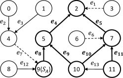
Figure 1: Example of a random RAPG instance: The graph $G=(V,E)$ contains $12$ nodes and $13$ directed edges each represented by an arrow. The random subgraph $g$ is obtained from $G$ by removing $3$ directed edges represented by dashed arrows, i.e., $e_{1}$, $e_{6}$ and $e_{7}$. From $g$ and the randomly selected “root” node $2$, we get the random RAPG instance $R=(V_{R},E_{R})$ where $V_{R}=\{2,5,7,9,10,11\}$ and $E_{R}=\{e_{4},e_{5},e_{8},e_{9},e_{10},e_{11}\}$.

Now we present the scoring system. For a random RAPG instance $R=(V_{R},E_{R})$ obtained from $v$ and $g\sim\mathcal{G}$, the score of a node set $S_{B}$ in $R$ is defined as follows.

Definition 4 (Score).

Suppose we are given a random RAPG instance $R=(V_{R},E_{R})$ obtained from $v$ and $g\sim\mathcal{G}$. The score of a node set $S_{B}$ in $R$, denoted by $f_{R}(S_{B}|S_{A})$, is defined as the probability that node $v$ will be influenced by source $B$ when 1) the influence propagates in graph $g$ with all edges being “active”; and 2) $S_{A}\cap V_{R}$ and $S_{B}\cap V_{R}$ are seed sets for source $A$ and $B$.

Recall that for the General Competitive Independent Cascade model, we assume that for any node $u\in V$, the conditional probability $\sigma_{u}(S_{B}|S_{A})$ is a monotone and submodular function of $S_{B}\subseteq V\backslash S_{A}$. It follows that, for any given $S_{A}$ and $R$, $f_{R}(S_{B}|S_{A})$ is also a monotone and submodular function of $S_{B}\subseteq V\backslash S_{A}$. Furthermore, we define the marginal gain of the score as follows.

Definition 5 (Marginal gain of score).

For a random RAPG instance $R$ with root $v$, we denote

$$\Delta_{R}(w|S_{A},S_{B})=f_{R}(S_{B}\cup\{w\}|S_{A})-f_{R}(S_{B}|S_{A})$$ (2)

as the marginal gain of score if we add $w$ to the seed set $S_{B}$.

From the definition of GCIC model and that of the RAPG, we know that for any RAPG instance $R$ obtained from $v$ and $g$, $R$ contains all nodes that can possibly influence $v$ and all shortest paths from these nodes to $v$. Hence, for any given $S_{A}$, $S_{B}$ and node $w$, once an instance $R$ is constructed, the evaluation of $f_{R}(S_{B}|S_{A})$ and $\Delta_{R}(w|S_{A},S_{B})$ can be done based on $R$ without the knowledge of $g$.

From Definition 4, for any $S_{B}\subseteq V\backslash S_{A}$, the expected value of $f_{R}(S_{B}|S_{A})$ over the randomness of $R$ equals to the probability that a randomly selected node in $G$ can be influenced by $S_{B}$. Formally, we have the following lemma.

Lemma 1.

For given seed set $S_{A}$ and $S_{B}$, we have

$$\sigma(S_{B}|S_{A})=n\cdot\mathbb{E}[f_{R}(S_{B}|S_{A})]$$ (3)

where the expectation of $n\cdot\mathbb{E}[f_{R}(S_{B}|S_{A})]$ is taken over the randomness of $R$, and $n$ is the number of nodes in $G$, or $n=|V|$.

Now we provide the Chernoff-Hoeffding bound in the form that we will frequently use throughout this paper.

Lemma 2 (Chernoff-Hoeffding Bound).

Let $X$ be the summation of $\theta$ i.i.d. random variables bounded in $[0,1]$ with a mean value $\mu$. Then, for any $\delta>0$,

$$\Pr[X>(1+\delta)\theta\mu] \leq\exp\Big{(}-\frac{\delta^{2}}{2+\delta}\cdot\theta\mu\Big{)},$$ (4)

$$\Pr[X<(1-\delta)\theta\mu] \leq\exp\Big{(}-\frac{\epsilon^{2}}{2}\cdot\theta\mu\Big{)}.$$ (5)

By Lemma 1 and Chernoff-Hoeffding bound, for a sufficiently large number of random RAPG instances, the average score of a set $S_{B}$ in those RAPG instances could be a good approximation to the expected influence of $S_{B}$ in $G$. The main challenge is how to determine the number of RAPG required, and how to select seed nodes for source $B$ based on a set of random RAPG instances. Similar to the work in [2], TCIM consists of two phases as follows.

1. Parameter estimation and refinement: Suppose $S_{B}^{*}$ is the optimal solution to the Competitive Influence Maximization Problem and let $OPT=\sigma(S_{B}^{*}|S_{A})$ be the expected influence of $S_{B}^{*}$ given $S_{A}$. In this phase, TCIM estimates and refines a lower bound of $OPT$ and uses the lower bound to derive a parameter $\theta$.

2. Node selection: In this phase, TCIM first generates a set $\mathcal{R}$ of $\theta$ random RAPG instances of $G$, where $\theta$ is a sufficiently large number obtained in the previous phase. Using the greedy approach, TCIM returns a set of seed nodes $S_{B}$ for source $B$ with the goal of maximizing $\sum_{R\in\mathcal{R}}f_{R}(S_{B}|S_{A})$.

IV-B Node Selection

Algorithm 1 shows the pseudo-code of the node selection phase. Given a graph $G$, the seed set $S_{A}$ of source $A$, the seed set size $k$ for source $B$ and a constant $\theta$, the algorithm returns a seed set $S_{B}$ of $k$ nodes for source $B$ with a large influence spread. In Line 1-2, the algorithm generates $\theta$ random RAPG instances and initializes $MG_{\mathcal{R}}(u):=\sum_{R\in\mathcal{R}}f_{R}(\{u\}|S_{A})$ for all nodes $u\in V\backslash S_{A}$. Then, in Line 3 - 13, the algorithm selects seed nodes $S_{B}$ iteratively using the greedy approach with the goal of maximizing $\sum_{R\in\mathcal{R}}f_{R}(S_{B}|S_{A})$.

Algorithm 1 NodeSelection $(G,S_{A},k,\theta)$

1:  Generate a set $\mathcal{R}$ of $\theta$ random RAPG instances.

2:  Let $MG_{\mathcal{R}}(u)=\sum_{R\in\mathcal{R}}f_{R}(\{u\}|S_{A})$ for all $u\in V\backslash S_{A}$.

3:  Initialize the seed set $S_{B}=\emptyset$.

4:  for $i=1$ to $k$ do

5:     Identity the node $v_{i}\!\in\!V\backslash(S_{A}\!\cup\!S_{B})$ with largest $MG_{\mathcal{R}}(v_{i})$.

6:     Add $v_{i}$ to $S_{B}$.

7:     if $i<k$ then

8:        // Update $MG_{\mathcal{R}}(u)$ as $\sum_{R\in\mathcal{R}}\Delta_{R}(u|S_{A},S_{B})$

9:        // for all $u\in V\backslash(S_{A}\cup S_{B})$.

10:        Let $\mathcal{R^{\prime}}\!=\!\{R|R\in\mathcal{R},\Delta_{R}(v_{i}|S_{A},S_{B}\backslash\{v_{i}\})>0\}$.

11:        for all $R\in\mathcal{R}^{\prime}$ and $u\in V_{R}\backslash(S_{A}\cup S_{B})$ do

12:           $MG_{\mathcal{R}}(u)=MG_{\mathcal{R}}(u)-\Delta_{R}(u|S_{A},S_{B}\backslash\{v_{i}\}).$

13:           $MG_{\mathcal{R}}(u)=MG_{\mathcal{R}}(u)+\Delta_{R}(u|S_{A},S_{B})$.

14:  return  $S_{B}$

Generation of RAPG instances. We adapt the randomized breadth-first search used in Borg et al.’s method [13] and Tang et al.’s algorithm [2] to generate random RAPG instances. We first randomly pick a node $r$ in $G$. Then, we create a queue containing a single node $r$ and initialize the RAPG instance under construction as $R=(V_{R}=\{r\},E_{R}=\emptyset)$. For all $u\in V$, let $d_{R}(u,r)$ be the shortest distance from $u$ to $r$ in the current $R$ and let $d_{R}(u,r)=+\infty$ if $u$ cannot reach $r$ in $R$. We iteratively pop the node $v$ at the top of the queue and examine its incoming edges. For each incoming neighbor $u$ of $v$ satisfying $d_{R}(u,r)\geq d_{R}(v,r)+1$, we generate a random number $l\!\in\![0,1]$. With probability $p_{uv}$ (i.e. $l\leq p_{uv}$), we insert $e_{uv}$ into $R$ and we push node $u$ into the queue if it has not been pushed into the queue before. If we push a node $u$ of $S_{A}$ into the queue while examining the incoming edge of a node $v$ with $d_{R}(v,r)=d$, we terminate the breadth-first search after we have examined incoming edges of all nodes whose distance to $r$ in $R$ is $d$. Otherwise, the breadth-first search terminates naturally when the queue becomes empty. If reverse the direction of all edges in $R$, we obtain an accessible pointed graph with “root” $r$, in which all nodes are reachable from $r$. For this reason, we refer to $r$ as the “root” of $R$.

Greedy approach. Let $F_{\mathcal{R}}(S_{B}|S_{A})=\sum_{R\in\mathcal{R}}f_{R}(S_{B}|S_{A})$ for all $S_{B}\subseteq V\backslash S_{A}$. Line 3-13 in Algorithm 1 uses the greedy approach to select a set of nodes $S_{B}$ with the goal of maximizing $F_{\mathcal{R}}(S_{B}|S_{A})$. Since the function $f_{R}(S_{B}|S_{A})$ is a monotone and submodular function of $S_{B}\subseteq V\backslash S_{A}$ for any RAPG instance $R$, we can conclude that $F_{\mathcal{R}}(S_{B}|S_{A})$ is also a monotone and submodular function of $S_{B}\subseteq V\backslash S_{A}$ for any $\mathcal{R}$. Hence, the greedy approach in Algorithm 1 could return a $(1-1/e)$ approximation solution [16]. Formally, let $S_{B}^{*}$ be the optimal solution, the greedy approach returns a solution $S_{B}$ such that $F_{\mathcal{R}}(S_{B}|S_{A})\geq(1-1/e)F_{\mathcal{R}}(S_{B}^{*}|S_{A})$.

The “marginal gain vector”. During the greedy selection process, we maintain a vector $MG_{\mathcal{R}}$ such that $MG_{\mathcal{R}}(u)=F_{\mathcal{R}}(S_{B}\cup\{u\}|S_{A})-F_{\mathcal{R}}(S_{B}|S_{A})$ holds for current $S_{B}$ and all $u\in V\backslash(S_{A}\cup S_{B})$. We refer to $MG_{\mathcal{R}}$ as the “marginal gain vector”. The initialization of $MG_{\mathcal{R}}$ could be done during or after the generation of random RAPG instances, whichever is more efficient. At the end of each iteration of the greedy approach, we update $MG_{\mathcal{R}}$. Suppose in one iteration, we expand the previous seed set $S_{B}^{\prime}$ by adding a node $v_{i}$ and the new seed set is $S_{B}=S_{B}^{\prime}\cup\{v_{i}\}$. For any RAPG instance $R$ such that $v_{i}\notin V_{R}$, we would have $\Delta_{R}(u|S_{A},S_{B}^{\prime})=\Delta_{R}(u|S_{A},S_{B})$ for all $u\in V\backslash(S_{A}\cup S_{B})$. And for any RAPG instance $R$ such that $f_{R}(S_{B}^{\prime}|S_{A})=1$, for all $u\in V\backslash(S_{A}\cup S_{B})$, we would have $\Delta_{R}(u|S_{A},S_{B}^{\prime})=0$ and the marginal gain of score cannot be further decreased. To conclude, for a given RAPG instance $R=(V_{R},E_{R})$ and a node $u\in V_{R}\backslash(S_{A}\cup S_{B})$, $\Delta_{R}(u|S_{A},S_{B})$ differs from $\Delta_{R}(u|S_{A},S_{B}^{\prime})$ only if $v_{i}\in V_{R}$ and $f_{R}(S_{B}^{\prime}|S_{A})<1$. Hence, to update $MG_{\mathcal{R}}(u)$ as $\sum_{R\in\mathcal{R}}\Delta_{R}(u|S_{A},S_{B})$ for all $u\in V\backslash(S_{A}\cup S_{B})$, it is not necessary to compute $\Delta_{R}(u|S_{A},S_{B})$ for all $R\in\mathcal{R}$ and $u\in V\backslash(S_{A}\cup S_{B})$. Note that for any RAPG instance $R$, $\Delta_{R}(v_{i}|S_{A},S_{B}\backslash\{v_{i}\})>0$ implies $v_{i}\in V_{R}$ and $f_{R}(S_{B}^{\prime}|S_{A})>1$. Therefore, Line 10-13 do the update correctly.

Time complexity analysis. Let $\mathbb{E}[N_{R}]$ be the expected number of random numbers required to generate a random RAPG instance, the time complexity of generating $\theta$ random RAPG instances is $O(\theta\cdot\mathbb{E}[N_{R}])$. Let $\mathbb{E}\left[|E_{R}|\right]$ be the expected number of edges in a random RAPG instance, which is no less than the expected number of nodes in a random RAPG instance. We assume that the initialization and update of $MG_{\mathcal{R}}$ takes time $O(c\theta\cdot\mathbb{E}\left[|E_{R}|\right])$. Here, $c=\Omega(1)$ depends on specific influence propagation model and may also depend on $k$ and $G$. In each iteration, we go through $MG_{\mathcal{R}}(u)$ for all nodes $u\in V\backslash(S_{A}\cup S_{B})$ and select a node with the largest value, which takes time $O(n)$. Hence, the total running time of Algorithm 1 is $O(kn+\theta\cdot\mathbb{E}[N_{R}]+c\theta\cdot\mathbb{E}\left[|E_{R}|\right])$. Moreover, from the fact that $\mathbb{E}\left[|E_{R}|\right]\leq\mathbb{E}[N_{R}]$ and $c=\Omega(1)$, the total running time can be written in a more compact form as

$$O(kn+c\theta\cdot\mathbb{E}[N_{R}]).$$ (6)

In Section V, we will show the value of $c$ and provide the total running time of the TCIM algorithm for several influence propagation models.

The Approximation guarantee. From Lemma 1, we see that the larger $\theta$ is, the more accurate is the estimation of the expected influence. The key challenge now becomes how to determine the value of $\theta$, i.e., the number of RAPG instances required, so to achieve certain accuracy of the estimation. More precisely, we would like to find a $\theta$ such that the node selection algorithm returns a $(1\!-\!1/e\!-\!\epsilon)$-approximation solution. At the same time, we also want $\theta$ to be as small as possible since it has the direct impact on the running time of Algorithm 1.

Using the Chernoff-Hoeffding bound, the following lemma shows that for a set $\mathcal{R}$ of sufficiently large number of random RAPG instances, $F_{\mathcal{R}}(S_{B}|S_{A})\cdot n/\theta=\left(\sum_{R\in\mathcal{R}}f_{R}(S_{B}|S_{A})\right)\cdot n/\theta$ could be an accurate estimate of the influence spread of $S_{B}$ given $S_{A}$, i.e., $\sigma(S_{B}|S_{A})$.

Lemma 3.

Suppose we are given a set $\mathcal{R}$ of $\theta$ random RAPG instances, where $\theta$ satisfies

$$\theta\geq(8+2\epsilon)n\cdot\frac{\ell\ln n+\ln\binom{n}{k}+\ln 2}{OPT\cdot\epsilon^{2}}.$$ (7)

Then, with probability at least $1-n^{-\ell}$,

$$\left|\frac{n}{\theta}\cdot F_{\mathcal{R}}(S_{B}|S_{A})-\sigma(S_{B}|S_{A})\right|<\frac{\epsilon}{2}OPT$$ (8)

holds for all $S_{B}\subseteq V\backslash S_{A}$ with $k$ nodes.

Proof.

First, let $S_{B}$ be a given seed set with $k$ nodes. Let $\mu=\mathbb{E}[f_{R}(S_{B}|S_{A})]$, $F_{\mathcal{R}}(S_{B}|S_{A})=\sum_{R\in\mathcal{R}}f_{R}(S_{B}|S_{A})$ can be regarded as the sum of $\theta$ i.i.d. variables with a mean $\mu$. By Lemma 1, we have $\mu=\sigma(S_{B}|S_{A})/n\leq OPT/n$. Thus, by Chernoff-Hoeffding bound,

$$\Pr\left[\left|\frac{n}{\theta}\cdot F_{\mathcal{R}}(S_{B}|S_{A})-\sigma(S_{B}|S_{A})\right|\geq\frac{\epsilon OPT}{2}\right]$$

$$= \Pr\left[\left|F_{\mathcal{R}}(S_{B}|S_{A})-\theta\cdot\mu\right|\geq\frac{\epsilon OPT}{2n\mu}\cdot\theta\mu\right]$$

$$\leq 2\exp\left(-\frac{(\frac{\epsilon OPT}{2n\mu})^{2}}{2+\frac{\epsilon OPT}{2n\mu}}\!\cdot\!\theta\mu\right)\!=\!2\exp\left(-\frac{\epsilon^{2}OPT^{2}}{8n^{2}\mu+2\epsilon nOPT}\!\cdot\!\theta\right)$$

$$\leq 2\exp\left(-\frac{\epsilon^{2}OPT}{(8+2\epsilon)\cdot n}\cdot\theta\right)\leq n^{-\ell}/\binom{n}{k}.$$

The last step follows by Inequality (7). There are at most $\binom{n}{k}$ node set $S_{B}\subseteq V\backslash S_{A}$ with $k$ nodes. By union bound, with probability at least $1-n^{-\ell}$, Inequality (8) holds for all $S_{B}\subseteq V\backslash S_{A}$ with $k$ nodes. ∎

For the value of $\theta$ in Algorithm 1, we have the following theorem.

Theorem 1.

Given that $\theta$ satisfies Inequality (7), Algorithm 1 returns a solution with $(1-1/e-\epsilon)$ approximation with probability at least $1-n^{-\ell}$.

Proof.

Suppose we are given a set $\mathcal{R}$ of $\theta$ random RAPG instances where $\theta$ satisfies Inequality (7). Let $S_{B}$ be the set of nodes returned by Algorithm 1 and let $S_{B}^{*}$ be the set that maximizes $F_{\mathcal{R}}(S_{B}^{*}|S_{A})$. As we are using a $(1-1/e)$ greedy approach to select $S_{B}$, we have $F_{\mathcal{R}}(S_{B}|S_{A})\geq(1-1/e)F_{\mathcal{R}}(S_{B}^{*}|S_{A})$.

Let $S_{B}^{\text{opt}}$ be the optimum seed set for source $B$, i.e., the set of nodes that maximizes the influence spread of $B$. We have $F_{\mathcal{R}}(S_{B}^{\text{opt}}|S_{A})\leq F_{\mathcal{R}}(S_{B}^{*}|S_{A})$.

By Lemma 3, with probability at least $1-n^{-\ell}$, we have $\sigma(S_{B}|S_{A})\geq F_{\mathcal{R}}(S_{B}|S_{A})\cdot n/\theta-OPT\cdot\epsilon/2$ holds simultaneously for all $S_{B}\subseteq V\backslash S_{A}$ with $k$ nodes.

Thus, we can conclude

$$\sigma(S_{B}|S_{A}) \geq\frac{n}{\theta}\cdot F_{\mathcal{R}}(S_{B}|S_{A})-\frac{\epsilon}{2}OPT$$

$$\geq\frac{n}{\theta}\cdot(1-1/e)F_{\mathcal{R}}(S_{B}^{*}|S_{A})-\frac{\epsilon}{2}OPT$$

$$\geq\frac{n}{\theta}\cdot(1-1/e)F_{\mathcal{R}}(S_{B}^{\text{opt}}|S_{A})-\frac{\epsilon}{2}OPT$$

$$\geq(1\!-\!1/e)(OPT\!-\!\frac{\epsilon}{2}OPT)\!-\!\frac{\epsilon}{2}OPT\geq(1\!-\!1/e\!-\!\epsilon)OPT,$$

which completes the proof. ∎

By Theorem 1, let $\lambda\!=\!(8+2\epsilon)n(\ell\ln n+\ln\binom{n}{k}+\ln 2)/\epsilon^{2}$, we know Algorithm 1 returns a $(1-1/e-\epsilon)$-approximate solution for any $\theta\geq\lambda/OPT$.

IV-C Parameter Estimation

The goal of our parameter estimation algorithm is to find a lower bound $LB_{e}$ of $OPT$ so that $\theta=\lambda/LB_{\text{e}}\geq\lambda/OPT$. Here, the subscript “e” of $LB_{\text{e}}$ is short for “estimated”.

Lower bound of $OPT$. We first define graph $G^{\prime}=(V,E^{\prime})$ as a subgraph of $G$ with all edges pointing to $S_{A}$ removed, i.e., $E^{\prime}\!=\!\{e_{uv}|e_{uv}\in E,v\in V\backslash S_{A}\}$. Let $m^{\prime}=|E^{\prime}|$. Then, we define a probability distribution $\mathcal{V^{+}}$ over the nodes in $V\backslash S_{A}$, such that the probability mass for each node is proportional to its number of incoming neighbors in $G^{\prime}$. Suppose we take $k$ samples from $\mathcal{V}^{+}$ and use them to form a node set $S_{B}^{+}$ with duplicated nodes eliminated. A natural lower bound of $OPT$ would be the expected influence spread of $S_{B}^{+}$ given the seeds for source $A$ is $S_{A}$, i.e., $\sigma(S_{B}^{+}|S_{A})$. Furthermore, any lower bound of $\sigma(S_{B}^{+}|S_{A})$ is also a lower bound of $OPT$. In the following lemma, we present a lower bound of $\sigma(S_{B}^{+}|S_{A})$.

Lemma 4.

Let $R$ be a random RAPG instance and let $V_{R}^{\prime}=\{u|u\in V_{R}\backslash S_{A},f_{R}(\{u\}|S_{A})=1\}$. We define the width of $R$, denoted by $w(R)$, as the number of edges in $G$ pointing to nodes in $V_{R}^{\prime}$. Then, we define

$$\alpha(R)=1-\left(1-\frac{w(R)}{m^{\prime}}\right)^{k}.$$ (9)

We have $n\cdot\mathbb{E}[\alpha(R)]\leq\sigma(S_{B}^{+}|S_{A})$, where the expectation of $\mathbb{E}[\alpha(R)]$ is taken over the randomness of $R$.

Proof.

Let $S_{B}^{+}$ be a set formed by $k$ samples from $\mathcal{V}^{+}$ with duplicated nodes eliminated and suppose we are given a random RAPG instance $R$. Let $p_{1}(R)$ be the probability that $S_{B}^{+}$ overlaps with $V_{R}^{\prime}$. For any $S_{B}^{+}$, we have $f_{R}(S_{B}^{+}|S_{A})\geq 0$ by definition of the scoring system. Moreover, if $S_{B}^{+}$ overlaps with $V_{R}^{\prime}$, we would have $f_{R}(S_{B}^{+}|S_{A})=1$. Hence, $p_{1}(R)\leq f_{R}(S_{B}^{+}|S_{A})$ holds and $n\cdot\mathbb{E}[p_{1}(R)]\leq n\cdot\mathbb{E}[f_{R}(S_{B}^{+}|S_{A})]=\sigma(S_{B}^{+}|S_{A})$ follows from Lemma 1. Furthermore, suppose we randomly select $k$ edges from $E^{\prime}$ and form a set $E^{+}$. Let $p_{2}(R)$ be the probability that at least one edge in $E^{+}$ points to a node in $V_{R}^{\prime}$. It can be verified that $p_{1}(R)=p_{2}(R)$. From the definition of $w(R)$, we have $p_{2}(R)=\alpha(R)=1-(1-w(R)/m^{\prime})^{k}$.

Therefore, we can conclude that

$$\mathbb{E}[\alpha(R)]=\mathbb{E}[p_{2}(R)]=\mathbb{E}[p_{1}(R)]\leq\sigma(S_{B}^{+}|S_{A})/n,$$

which completes the proof. ∎

Let $LB_{\text{e}}:=n\cdot\mathbb{E}[\alpha(R)]$. Then, Lemma 4 shows that $LB_{\text{e}}$ is a lower bound of $OPT$.

Estimation of the lower bound. By Lemma 4, we can estimate $LB_{\text{e}}$ by first measuring $n\cdot\alpha(R)$ on a set of random RAPG instances and then take the average of the estimation. By Chernoff-Hoeffding bound, to obtain an estimation of $LB_{\text{e}}$ within $\delta\in[0,1]$ relative error with probability at least $1-n^{-\ell}$, the number of measurements required is $\Omega(n\ell\log n\epsilon^{-2}/LB_{\text{e}})$. The difficulty is that we usually have no prior knowledge about $LB_{\text{e}}$. In [2], Tang et al. provided an adaptive sampling approach which dynamically adjusts the number of measurements based on the observed sample value. Suppose $S_{A}=\emptyset$, the lower bound $LB_{\text{e}}$ we want to estimate equals to the lower bound of maximum influence spread estimated in [2]. Hence, we apply Tang et al.’s approach directly and Algorithm 2 shows the pseudo-code that estimates $LB_{\text{e}}$.

Algorithm 2 EstimateLB$(G,\ell)$ [2]

1:  for $i=1$ to $\log_{2}n-1$ do

2:     Let $c_{i}=(6\ell\ln n+6\ln(\log_{2}n))\cdot 2^{i}$.

3:     Let $s_{i}=0$.

4:     for $j=1$ to $c_{i}$ do

5:        Generate a random RAPG instance $R$ and calculate $\alpha(R)$.

6:        Update $s_{i}=s_{i}+\alpha(R)$.

7:     if $s_{i}>c_{i}/2^{i}$ then

8:        return  $LB_{\text{e}}^{*}=n\cdot s_{i}/(2\cdot c_{i})$.

9:  return  $LB_{\text{e}}^{*}=1$.

For Algorithm 2, the theoretical analysis in [2] can be applied directly and the following theorem holds. For the proof of Theorem 2, we refer interested readers to [2].

Theorem 2.

When $n\geq 2$ and $\ell\geq 1/2$, Algorithm 2 returns $LB_{\text{e}}^{*}\in[LB_{\text{e}}/4,OPT]$ with at least $1-n^{-\ell}$ probability, and has expected running time $O(\ell(m+n)\log n)$. Furthermore, $\mathbb{E}[1/LB_{\text{e}}^{*}]<12/LB_{\text{e}}$.

Running time of the node selection process. We have shown how to estimate a lower bound of $OPT$, now we analyze Algorithm 1 assuming $\theta\!=\!\lambda/LB_{\text{e}}^{*}$. From $\theta\!\geq\!\lambda/OPT$ and Theorem 1, we know Algorithm 1 returns a $(1-1/e-\epsilon)$-approximate solution with high probability. Now we analyze the running time of Algorithm 1. The running time of building $\theta$ random RAPG instances is $O(\theta\cdot\mathbb{E}[N_{R}])=O(\frac{\lambda}{LB_{\text{e}}^{*}}\cdot\mathbb{E}[N_{R}])$ where $\mathbb{E}[N_{R}]$ is the expected number of random numbers generated for building a random RAPG instance. The following lemma shows the relationshp between $LB_{\text{e}}$ and $\mathbb{E}[N_{R}]$.

Lemma 5.

$LB_{\text{e}}\geq\frac{n}{m}\mathbb{E}[N_{R}]$.

Proof.

For a given RAPG instance $R$, recall that $w(R)$ is defined as the number of edges in $G$ pointing to any node $u\in V$ such that $u\in V\backslash S_{A}$ and $f_{R}(\{u\}|S_{A})=1$. If we generate a random number for an edge $e_{uv}\in E$ during the generation of $R$, we know $v\in V\backslash S_{A}$ and $f_{R}(\{v\}|S_{A})=1$. Hence, the number of random number generated during the generation of $R$ is no more than $w(R)$ and we have $\mathbb{E}[N_{R}]\leq\mathbb{E}[w(R)]$. Moreover, we can conclude that

$$\frac{n}{m}\mathbb{E}[N_{R}]\leq n\cdot\mathbb{E}\left[\frac{w(R)}{m}\right]\leq n\cdot\sum_{R}\left(\Pr(R)\cdot\frac{w(R)}{m^{\prime}}\right)$$

$$\leq n\cdot\sum_{R}\left(\Pr(R)\cdot\alpha(R)\right)=n\cdot\mathbb{E}[\alpha(R)],$$

which completes the proof. ∎

Based on Theorem 2 showing $\mathbb{E}[1/LB_{\text{e}}^{*}]=O(1/LB_{\text{e}})$ and Lemma 5 showing $LB_{\text{e}}\geq\mathbb{E}[N_{R}]\cdot n/m$, we can conclude that $\mathbb{E}\left[\mathbb{E}[N_{R}]/LB_{\text{e}}^{*}\right]=O(1+m/n)$. Recall that the greedy selection process in Algorithm 1 has time complexity $O(kn+c\theta\cdot\mathbb{E}[N_{R}])$. Let $\theta=\lambda/LB_{\text{e}}^{*}$, the total running time of Algorithm 1 becomes $O\big{(}kn\!+\!c\lambda\mathbb{E}[N_{R}]/LB_{\text{e}}^{*}\big{)}\!=\!O\left(c(\ell\!+\!k)(m\!+\!n)\log n/\epsilon^{2}\right)$.

IV-D Parameter Refinement

As discussed before, if the lower bound of $OPT$ is tight, our algorithm will have a short running time. The current lower bound $LB_{\text{e}}$ is no greater than the expected influence spread of a set of $k$ independent samples from $\mathcal{V^{+}}$, with duplicated eliminated. Hence, $LB_{\text{e}}$ is often much smaller than the $OPT$. To narrow the gaps between the lower bound we get in Algorithm 2 and $OPT$, we use a greedy algorithm to find a seed set $S_{B}^{\prime}$ based on the limited number of RAPG instances we have already generated in Algorithm 2, and estimate the influence spread of $S_{B}^{\prime}$ with a reasonable accuracy. Then, the intuition is that we can use a creditable lower bound of $\sigma(S_{B}^{\prime}|S_{A})$ or $LB_{\text{e}}^{*}$, whichever is larger, as the refined bound.

Algorithm 3 describes how to refine the lower bound. Line 2-8 uses the greedy approach to find a seed set $S_{B}^{\prime}$ based on the RAPG instances generated in Algorithm 2. Intuitively, $S_{B}^{\prime}$ should have a large influence spread when used as seed set for source $B$. Line 9-13 estimates the expected influence of $S_{B}^{\prime}$, i.e. $\sigma(S_{B}^{\prime}|S_{A})$. By Lemma 1, let $\mathcal{R^{\prime\prime}}$ be a set of RAPG instances, $F:=n\cdot\left(\sum_{R\in\mathcal{R^{\prime\prime}}}f_{R}(S_{B}^{\prime}|S_{A})\right)/|\mathcal{R^{\prime\prime}}|$ is an unbiased estimation of $\sigma(S_{B}^{\prime}|S_{A})$. Algorithm 3 generates a sufficiently large number of RAPG instances and put them into $\mathcal{R^{\prime\prime}}$ such that $F\leq(1+\epsilon^{\prime})\sigma(S_{B}^{\prime}|S_{A})$ holds with high probability. Then, with high probability, we have $F/(1+\epsilon^{\prime})\leq\sigma(S_{B}^{\prime}|S_{A})\leq OPT$. We use $LB_{\text{r}}=\max\{F/(1+\epsilon^{\prime}),LB_{\text{e}}^{*}\}$ as the refined lower bound of $OPT$, which will be used to derive $\theta$ in Algorithm 1. The subscript “r” of $LB_{\text{r}}$ stands for “refinement”.

Algorithm 3 RefineLB$(G,k,S_{A},LB_{\text{e}}^{*},\epsilon,\ell)$

1:  Let $\mathcal{R^{\prime}}$ be the set of RAPG instances generated in Algorithm 2.

2:  Let $MG_{\mathcal{R^{\prime}}}(u)=\sum_{R\in\mathcal{R^{\prime}}}f_{R}(\{u\}|S_{A})$ for all $u\in V\backslash S_{A}$.

3:  Initialize the seed set $S_{B}^{\prime}=\emptyset$.

4:  for $i=1$ to $k$ do

5:     Identity the node $v_{i}\!\in\!V\backslash(S_{A}\cup S_{B})$ with largest $MG_{\mathcal{R^{\prime}}}(v_{i})$.

6:     Add $v_{i}$ to $S_{B}^{\prime}$.

7:     if $i<k$ then

8:        Update $MG_{\mathcal{R^{\prime}}}(u)$ as $\sum_{R\in\mathcal{R}}\Delta_{R}(u|S_{A},S_{B})$ for all $u\in V\backslash(S_{A}\cup S_{B})$.

9:  $\epsilon^{\prime}=5\cdot\sqrt[3]{\ell\cdot\epsilon^{2}/(\ell+k)}$

10:  $\lambda^{\prime}=(2+\epsilon^{\prime})\ell n\ln n/\epsilon^{\prime 2}$

11:  $\theta^{\prime}=\lambda^{\prime}/LB_{\text{e}}^{*}$

12:  Generate a set $\mathcal{R^{\prime\prime}}$ of $\theta^{\prime}$ random RAPG instances.

13:  Let $F=n\cdot\left(\sum_{R\in\mathcal{R^{\prime\prime}}}f_{R}(S_{B}^{\prime}|S_{A})\right)/\theta^{\prime}$.

14:  return  $LB_{\text{r}}=\max\{F/(1+\epsilon^{\prime}),LB_{\text{e}}^{*}\}$

Theoretical analysis. We now prove that Algorithm 3 returns $LB_{\text{r}}\in[LB_{\text{e}}^{*},OPT]$ with a high probability.

Lemma 6.

If $LB_{\text{e}}^{*}\in[LB_{\text{e}}/4,OPT]$, Algorithm 3 returns $LB_{\text{r}}\in[LB_{\text{e}}^{*},OPT]$ with at least $1-n^{-\ell}$ probability.

Proof.

As $LB_{\text{r}}=\max\{F/(1+\epsilon^{\prime}),LB_{\text{e}}^{*}\}$ and $LB_{\text{e}}^{*}\leq OPT$, it is suffice to show $F/(1+\epsilon^{\prime})\leq OPT$ holds with probability at least $1-n^{-\ell}$. By Line 13 in Algorithm 3, we know $F/(1+\epsilon^{\prime})\leq OPT$ if and only if $\sum_{R\in\mathcal{R^{\prime\prime}}}f_{R}(S_{B}^{\prime}|S_{A})\leq OPT\cdot\theta^{\prime}(1+\epsilon^{\prime})/n$. Let $\mu=\mathbb{E}[f_{R}(S_{B}^{\prime}|S_{A})]$, by Lemma 1, we have $n\mu=\sigma(S_{B}^{\prime}|S_{A})\leq OPT$. Since $\sum_{R\in\mathcal{R^{\prime\prime}}}f_{R}(S_{B}^{\prime}|S_{A})$ is the summation of $|\mathcal{R}^{\prime\prime}|=\theta^{\prime}$ i.i.d. random variable with mean $\mu$, By $n\mu\leq OPT$, $LB_{\text{e}}^{*}\leq OPT$ and Chernoff bound,

$$\Pr\left[\sum_{R\in\mathcal{R^{\prime\prime}}}f_{R}(S_{B}^{\prime}|S_{A})\geq\frac{OPT(1+\epsilon^{\prime})}{n}\cdot\theta^{\prime}\right]$$

$$\leq \Pr\left[\sum_{R\in\mathcal{R^{\prime\prime}}}f_{R}(S_{B}^{\prime}|S_{A})-\mu\theta^{\prime}\geq\frac{OPT\epsilon^{\prime}}{n\mu}\cdot\mu\theta^{\prime}\right]$$

$$\leq \exp\left(-\frac{\left(\frac{OPT\epsilon^{\prime}}{n\mu}\right)^{2}}{2+\frac{OPT\epsilon^{\prime}}{n\mu}}\cdot\mu\theta^{\prime}\right)\!=\!\exp\left(-\frac{OPT^{2}\epsilon^{\prime 2}}{2n^{2}\mu+OPT\epsilon^{\prime}n}\cdot\theta^{\prime}\right)$$

$$\leq \exp\left(-\frac{OPT\epsilon^{\prime 2}}{(2+\epsilon^{\prime})n}\cdot\frac{\lambda^{\prime}}{LB_{\text{e}}^{*}}\right)\leq\exp\left(-\frac{\epsilon^{\prime 2}\lambda^{\prime}}{(2+\epsilon^{\prime})n}\right)\leq\frac{1}{n^{\ell}}.$$

The last inequality holds since $\lambda^{\prime}=(2+\epsilon^{\prime})\ell n\ln n/\epsilon^{\prime 2}$ and this completes the proof. ∎

Time complexity. We now analyze the time complexity of Algorithm 3. The running time of Line 2-8 depends on $|\mathcal{R^{\prime}}|$. Theorem 2 shows that the expected running time of Algorithm 2 is $O(\ell(m+n)\log n)$, which means that the total number of edges in all RAPG instances is at most $O(\ell(m+n)\log n)$. Hence, in Lines 2-8 of Algorithm 3, the running time for the initialization and update of $MG_{\mathcal{R^{\prime}}}$ would be $O(c\ell(m+n)\log n)$. And the running time of Line 2-8 would be $O(c\ell(m+n)\log n+kn)=O(c(\ell+k)(m+n)\log n)$. The running time of the Line 9-13 is $O\left(\mathbb{E}[\lambda^{\prime}/LB_{\text{e}}^{*}]\cdot\mathbb{E}[N_{R}]\right)$, because we generate $\lambda^{\prime}/LB_{\text{e}}^{*}$ RAPG instances and the running time of calculating $f_{R}(S_{B}^{\prime}|S_{A})$ for an RAPG instance $R=(V_{R},E_{R})$ is linear with $|V_{R}|$. As $\mathbb{E}[1/LB_{\text{e}}^{*}]=O(12/LB)$ holds from Theorem 2 and $\frac{n}{m}\mathbb{E}[N_{R}]\leq LB_{\text{e}}$ holds from Lemma 5, we can conclude that

$$O\left(\mathbb{E}\left[\frac{\lambda^{\prime}}{LB_{\text{e}}^{*}}\right]\cdot\mathbb{E}[N_{R}]\right) =O\left(\frac{\lambda^{\prime}}{LB_{\text{e}}}\cdot\mathbb{E}[N_{R}]\right)$$

$$=O\left(\frac{\lambda^{\prime}}{LB_{\text{e}}}\cdot\left(1+\frac{m}{n}\right)LB_{\text{e}}\right)=O(\ell(m+n)\log n/\epsilon^{\prime 2}).$$

To make sure that Algorithm 3 has the same time complexity as Algorithm 1, the value of $\epsilon^{\prime}$ must satisfy $\epsilon^{\prime}\geq\sqrt{\ell/(c(\ell+k))}\cdot\epsilon$. In TIM/TIM⁺ [2] that returns approximation solution for single source influence maximization problem under the IC model, Tang et al. set $\epsilon^{\prime}=5\sqrt[3]{\ell\cdot\epsilon^{2}/(k+\ell)}$ for any $\epsilon\leq 1$. Note that for a special case of the General Competitive Independent Cascade model where $S_{A}=\emptyset$, the influence propagation model is actually the single source IC model. Hence, we also set $\epsilon^{\prime}=5\sqrt[3]{\ell\cdot\epsilon^{2}/(k+\ell)}$ for any $\epsilon\leq 1$. Note that $c\geq 1$, it could be verified that $5\sqrt[3]{\ell\cdot\epsilon^{2}/(k+\ell)}\geq\sqrt{\ell/(c(\ell+k))}\epsilon$ holds for any $\epsilon\leq 1$. Based on Lemma 6 and the time complexity analysis above, we have the following Theorem.

Theorem 3.

Given $\mathbb{E}[1/LB_{\text{e}}^{*}]=O(12/LB_{\text{e}})$ and $LB_{\text{e}}^{*}\in[LB_{\text{e}}/4,OPT]$, Algorithm 3 returns $LB_{\text{r}}\in[LB_{\text{e}}^{*},OPT]$ with at least $1-n^{-\ell}$ probability and runs in $O(c(m+n)(\ell+k)\log n/\epsilon^{2})$ expected time.

If $LB_{\text{r}}\geq LB_{\text{e}}^{*}$, let $\theta=\lambda/LB_{\text{r}}$, the total running time of Algorithm 1 is still $O(c(\ell+k)(m+n)\log n/\epsilon^{2})$.

IV-E TCIM as a whole

Now we are in the position to put Algorithm 1-3 together and present the complete TCIM algorithm. Given a network $G$, the seed set $S_{A}$ for the source $A$ together with parametric values $k$, $\ell$ and $\epsilon$, TCIM returns a $(1-1/e-\epsilon)$ solution with probability at least $1-n^{-\ell}$. First, Algorithm 2 returns the estimated lower bound of $OPT$, denoted by $LB_{\text{e}}^{*}$. Then, we feed $LB_{\text{e}}^{*}$ to Algorithm 3 and get a refined lower bound $LB_{\text{r}}$. Finally, Algorithm 1 returns a set $S_{B}$ of $k$ seeds for source $B$ based on $\theta=\lambda/LB_{\text{r}}$ random RAPG instances. Algorithm 4 describes the pseudo-code of TCIM as a whole.

Algorithm 4 TCIM $(G,S_{A},k,\ell,\epsilon)$

1:  $\ell^{\prime}=\ell+\ln 3/\ln n$

2:  $LB_{\text{e}}^{*}=\text{EstimateLB}(G,\ell^{\prime})$

3:  $LB_{\text{r}}=\text{RefineLB}(G,k,S_{A},LB_{\text{e}}^{*},\epsilon,\ell^{\prime})$

4:  $\lambda=(8+2\epsilon)n\left(\ell^{\prime}\ln n+\ln\binom{n}{k}+\ln 2\right)/\epsilon^{2}$

5:  $\theta=\lambda/LB_{\text{r}}$

6:  $S_{B}=\text{NodeSelection}(G,S_{A},k,\theta)$

7:  return  $S_{B}$

We use $\ell^{\prime}=\ell+\ln 3/\ln n$ as the input parameter value of $\ell$ for Algorithm 1-3. By setting this, Algorithm 1-3 each fails with probability at most $n^{-\ell}/3$. Hence, by union bound, TCIM succeeds in returning a $(1-1/e-\epsilon)$ approximation solution with probability at least $1-n^{-\ell}$. Moreover, the total running time of TCIM is $O(c(\ell+k)(m+n)\log n/\epsilon^{2})$, because Algorithm 1-3 each takes time at most $O(c(\ell+k)(m+n)\log n/\epsilon^{2})$. In conclusion, we have the following theorem.

Theorem 4 (TCIM).

TCIM returns $(1-1/e-\epsilon)$-approximate solution with probability at least $1-n^{-\ell}$. The time complexity is $O(c(\ell+k)(m+n)\log n/\epsilon^{2})$.

V Analyzing Various Propagation Models under GCIC

In this section, we describe some special cases of the GCIC model and provide detailed analysis about TCIM for these models. To show the generality of the GCIC model, we use the Campaign-Oblivious Independent Cascade Model in [6], the Distance-based model and Wave propagation model in [4] as specific propagation models. For each specific model, we first briefly describe how the influence propagates, give examples of score in a simple RAPG instance as shown in Figure 2, and analyze the time complexity of the TCIM algorithm.

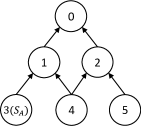
Figure 2: Example of a random RAPG instance with $6$ nodes and $6$ edges. Node $3$ is a seed of source $A$.

V-A Campaign-Oblivious Independent Cascade model

Budak et al. [6] introduced the Campaign-Oblivious Independent Cascade model (COICM) extending the single source IC model. The influence propagation process starts with two sets of active nodes $S_{A}$ and $S_{B}$, and then unfolds in discrete steps. At step $0$, nodes in $S_{A}$ (resp. $S_{B}$) are activated and are in state $I_{A}$ (resp. $I_{B}$). When a node $u$ first becomes activated in step $t$, it gets a single chance to activate each of its currently uninfluenced neighbor $v$ and succeeds with the probability $p_{uv}$. Budak et al. assumed that one source is prioritized over the other one in the propagation process, and nodes influence by the dominant source always attempt to influenced its uninfluenced neighbors first. Here we assume that if there are two or more nodes trying to activate a node $v$ at a given time step, nodes in state $I_{B}$ (i.e., nodes influenced by source $B$) attempt first, which means source $B$ is prioritized over source $A$.

Examples of score. Suppose we are given seed sets $S_{A}$ and $S_{B}$ and a set of active edges $E_{a}$. In COICM, a node $u$ will be influenced by source $B$ if and only if $d_{u}(S_{B},E_{a})=d_{u}(S_{A}\cup S_{B},E_{a})$. For the RAPG instance $R$ in Figure 2, $f_{R}(S_{B}|S_{A})=1$ if $S_{B}\cap\{0,1,2,4,5\}\neq\emptyset$ and $f_{R}(S_{B}|S_{A})=0$ otherwise.

Analysis of TCIM algorithm. Recall that while analyzing the running time of TCIM, we assume that if we have a set $\mathcal{R}$ of $\theta$ RAPG instances, the time complexity for the initialization and update of the “marginal gain vector” $MG_{\mathcal{R}}$ is $O(c\theta\cdot\mathbb{E}\left[|E_{R}|\right])$. We now show that $c=O(1)$ for COICM. Suppose we are selecting nodes based on a set $\mathcal{R}$ of $\theta$ RAPG instances. The initialization of $MG_{\mathcal{R}}$ takes time $O(\theta\cdot\mathbb{E}\left[|E_{R}|\right])$ as for any RAPG instance $R$, we have $f_{R}(\{u\}|S_{A})=1$ for all $u\in V_{R}\backslash S_{A}$ and $f_{R}(\{u\}|S_{A})=0$ otherwise. Suppose in one iteration, we add a node $v_{i}$ to the set $S_{B}^{\prime}$ and obtain a new seed set $S_{B}=S_{B}^{\prime}\cup\{v_{i}\}$. Recall that we define $\mathcal{R^{\prime}}=\{R|R\in\mathcal{R},\Delta_{R}(v_{i}|S_{A},S_{B}^{\prime})\}$ in the greedy approach. For every RAPG instance $R\in\mathcal{R^{\prime}}$ and for all $u\in V\backslash(S_{A}\cup S_{B})$, we would have $\Delta_{R}(u|S_{A},S_{B})=0$ and $\Delta_{R}(u|S_{A},S_{B}^{\prime})=1$ and hence we need to update $MG_{\mathcal{R}}(u)$ correspondingly. For each RAPG instance $R$, it appears in $\mathcal{R^{\prime}}$ in at most one iteration. Hence, the total time complexity of the initialization and update of the “marginal gain vector” takes time $O(\theta\cdot\mathbb{E}\left[|E_{R}|\right])$. It follows that the running time of TCIM is $O((\ell+k)(m+n)\log n/\epsilon^{2})$.

V-B Distance-based Model

Carnes et al. proposed the Distance-based model in [4]. The idea is that a consumer is more likely to be influenced by the early adopters if their distance in the network is small. The model governs the diffusion of source $A$ and $B$ given the initial adopters for each source and a set $E_{a}\subseteq E$ of active edges. Let $d_{u}(E_{a},S_{A}\cup S_{B})$ be the shortest distance from $u$ to $S_{A}\cup S_{B}$ along edges in $E_{a}$ and let $d_{u}(E_{a},S_{A}\cup S_{B})=+\infty$ if there are no paths from $u$ to any node in $S_{A}\cup S_{B}$. For any set $S\subseteq V$, we define $h_{u}(S,d_{u}(E_{a},S_{A}\cup S_{B}))$ as the number of nodes in $S$ at distance $d_{u}(E_{a},S_{A}\cup S_{B})$ from $u$ along edges in $E_{a}$. Given $S_{A}$, $S_{B}$ and a set of active edge $E_{a}$, the probability that node $u$ will be influenced by source $B$ is

$$\frac{h_{u}(S_{B},d_{u}(E_{a},S_{A}\!\cup\!S_{B}))}{h_{u}(S_{A}\!\cup\!S_{B},d_{u}(E_{a},S_{A}\!\cup\!S_{B}))}.$$ (10)

Thus, the expected influence of $S_{B}$ is

$$\sigma(S_{B}|S_{A})\!=\!\mathbb{E}\left[\sum_{u\in V}\frac{h_{u}(S_{B},d_{u}(E_{a},S_{A}\!\cup\!S_{B}))}{h_{u}(S_{A}\!\cup\!S_{B},d_{u}(E_{a},S_{A}\!\cup\!S_{B}))}\right],$$ (11)

where the expectation is taken over the randomness of $E_{a}$.

Examples of the score. Suppose we are given a random RAPG instance $R$ shown in Figure 2. If $S_{B}\cap\{0,1,2\}\neq\emptyset$, we would have $f_{R}(S_{B}|S_{A})=1$. Suppose $S_{B}=\{4,5\}$, we have $d_{0}(E_{R},S_{A}\cup S_{B})=2$, $h_{0}(S_{B},2)=2$ and $h_{0}(S_{A}\cup S_{B},2)=3$. Hence the probability that node $0$ will be influenced by source $B$ is $\frac{2}{3}$ and we have $f_{R}(S_{B}=\{4,5\}|S_{A})=\frac{2}{3}$. For $S_{B}=\{4\}$ or $S_{B}=\{5\}$, one can verify that $f_{R}(S_{B}|S_{A})=\frac{1}{2}$.

Analysis of TCIM algorithm. We now show that $c=O(k)$ for the Distance-based Model. In the implementation of TCIM under the Distance-based Model, for each RAPG instance $R=(V_{R},E_{R})$ with “root” $r$, we keep $d_{R}(v,r)$ for all $v\in V_{R}$ and $d_{R}(S_{A},r)$ in the memory. Moreover, we keep track of the value $h_{r}(S_{A}\cup S_{B},d_{R}(S_{A},r))$ and $h_{r}(S_{B},d_{R}(S_{A},r))$ for current $S_{B}$ and put them inside the memory. Then, for any given RAPG instance $R=(V_{R},E_{R})$ and a node $u\in V_{R}\backslash(S_{A}\cup S_{B})$, we have

$$f_{R}(S_{B}\cup\{u\}|S_{A})=\frac{h_{r}(S_{B},d_{R}(S_{A},r))+1}{h_{r}(S_{A}\cup S_{B},d_{R}(S_{A},r))+1}$$

if $d_{R}(u,r)=d_{R}(S_{A},r)$ and $f_{R}(S_{B}\cup\{u\}|S_{A})=1$ otherwise. In each iteration, for each RAPG instance $R$, the update of $h_{r}(S_{A}\cup S_{B},d_{R}(S_{A},r))$ and $h_{r}(S_{B},d_{R}(S_{A},r))$ after expanding previous seed set $S_{B}$ by adding a node could be done in $O(1)$. Moreover, for any $R$ and $u\in V_{R}\backslash(S_{A}\cup S_{B})$, the evaluation of $\Delta_{R}(u|S_{A},S_{B})$ could also be done in $O(1)$. There are $O(\theta)$ RAPG instances with the total number of nodes being $O(\theta\cdot\mathbb{E}\left[|E_{R}|\right])$. Hence, in $k$ iterations, it takes $O(k\theta\cdot\mathbb{E}\left[|E_{R}|\right])$ in total to initialize and update the marginal gain vector. Substituting $c$ with $O(k)$ in $O(c(\ell+k)(m+n)\log n/\epsilon^{2})$, the running time of the TCIM algorithm is $O(k(\ell+k)(m+n)\log n/\epsilon^{2})$.

V-C Wave Propagation Model

Carnes et al. also proposed the Wave Propagation Model in [4] extending the single source IC model. Suppose we are given $S_{A}$, $S_{B}$ and a set of active edges $E_{a}$, we denote $p(u|S_{A},S_{B},E_{a})$ as the probability that node $u$ gets influenced by source $B$. We also let $d_{E_{a}}(S_{A}\cup S_{B},u)$ be the shortest distance from seed nodes to $u$ through edges in $E_{a}$. Let $N_{u}$ be the set of neighbors of $u$ whose shortest distance from seed nodes through edges in $E_{a}$ is $d_{E_{a}}(S_{A}\cup S_{B},u)-1$. Then, Carnes et al. [4] defines

$$p(u|S_{A},S_{B},E_{a})=\frac{\sum_{v\in N_{u}}p(v|S_{A},S_{B},E_{a})}{|N_{u}|}.$$ (12)

The expected number of nodes $S_{B}$ can influence given $S_{A}$ is

$$\sigma(S_{B}|S_{A})=\mathbb{E}\left[\sum\limits_{v\in V}p(v|S_{A},S_{B},E_{a})\right],$$ (13)

where the expectation is taken over the randomness of $E_{a}$.

Examples of score. For a random RAPG instance $R$ shown in Figure 2, as for the Distance-based Model, we have $f_{R}(S_{B}|S_{A})=1$ if $S_{B}\cap\{0,1,2\}\neq\emptyset$. Suppose $S_{B}=\{4\}$, source $B$ would influence node $4$ and $2$ with probability $1$, influence node $1$ with probability $\frac{1}{2}$ and influence node $0$ with probability $\frac{3}{4}$. Hence, $f_{R}(\{4\}|S_{A})=\frac{3}{4}$. Suppose $S_{B}=\{5\}$, source $B$ would influence node $5$ and $2$ with probability $1$, influence node $0$ with probability $\frac{1}{2}$. Hence, $f_{R}(\{5\}|S_{A})=\frac{1}{2}$. Moreover, one can verify that $f_{R}(\{4,5\}|S_{A})=\frac{3}{4}$.

Analysis of TCIM algorithm. We now show that for a greedy approach based on a set of $\theta$ random RAPG instances, it takes $O(kn\cdot\theta\cdot\mathbb{E}[N_{R}])$ in total to initialize and update the “marginal gain vector”. In each iteration of the greedy approach, for each RAPG instance $R=(V_{R},E_{R})$ and each node $u\in V_{R}\backslash(S_{A}\cup S_{B})$, it takes $O(|E_{R}|)\leq O(\mathbb{E}[N_{R}])$ to update the marginal gain vector. Since there are $\theta$ RAPG instances each having at most $n$ nodes and the greedy approach runs in $k$ iteration, it takes at most $O(kn\cdot\theta\cdot\mathbb{E}[N_{R}])$ in total to initialize and update the marginal gain vector. Substituting $c=O(kn)$ into $O(c(\ell+k)n(m+n)\log n/\epsilon^{2})$, we can conclude that the running time of TCIM is $O(k(\ell+k)n(m+n)\log n/\epsilon^{2})$.

VI Comparison with the Greedy Algorithm

In this section, we compare TCIM to the greedy approach with Monte-Carlo method. We denote the greedy algorithm as GreedyMC, and it works as follows. The seed set $S_{B}$ is set to be empty initially and the greedy selection approach runs in $k$ iterations. In the $i$-th iteration, GreedyMC identifies a node $v_{i}\in V\backslash(S_{A}\cup S_{B})$ that maximizes the marginal gain of influence spread of source $B$, i.e., maximizes $\sigma(S_{B}\cup\{v_{i}\}|S_{A})-\sigma(S_{B}|S_{A})$, and put it into $S_{B}$. Every estimation of the marginal gain is done by $r$ Monte-Carlo simulations. Hence, GreedyMC runs in at least $O(kmnr)$ time.

In [2], Tang et al. provided the lower bound of $r$ that ensures the $(1-1/e-\epsilon)$ approximation ratio of this method for single source influence maximization problem. We extend their analysis on GreedyMC and give the following theorem.

Theorem 5.

For the Competitive Influence Maximization problem, GreedyMC returns a $(1-1/e-\epsilon)$-approximate solution with at least $1\!-\!n^{-\ell}$ probability, if

$$r\geq(8k^{2}+2k\epsilon)\cdot n\cdot\frac{(\ell+1)\ln n+\ln k}{\epsilon^{2}\cdot OPT}.$$ (14)

Proof.

Let $S_{B}$ be any node set that contains at most $k$ nodes in $V\backslash S_{A}$ and let $\sigma^{\prime}(S_{B}|S_{A})$ be the estimation of $\sigma(S_{B}|S_{A})$ computed by $r$ Monte-Carlo simulations. Then, $r\sigma^{\prime}(S_{B}|S_{A})$ can be regarded as the sum of $r$ i.i.d. random variable bounded in $[0,1]$ with the mean value $\sigma(S_{B}|S_{A})$. By Chernoff-Hoeffding bound, if $r$ satisfies Ineq. (14), it could be verified that $\Pr\left[|\sigma^{\prime}(S_{B}|S_{A})-\sigma(S_{B}|S_{A})|>\frac{\epsilon}{2k}OPT\right]$ is at least $k^{-1}\cdot n^{-(\ell+1)}$. Given $G$ and $k$, GreedyMC considers at most $kn$ node sets with sizes at most $k$. Applying the union bound, with probability at least $1-n^{-\ell}$, we have

$$|\sigma^{\prime}(S_{B}|S_{A})-\sigma(S_{B}|S_{A})|>\frac{\epsilon}{2k}\cdot OPT$$ (15)

holds for all sets $S_{B}$ considered by the greedy approach. Under the assumption that $\sigma^{\prime}(S_{B}|S_{A})$ for all set $S_{B}$ considered by GreedyMC satisfies Inequality (15), GreedyMC returns a $(1-1/e-\epsilon)$-approximate solution. For the detailed proof of the accuracy of GreedyMC, we refer interested readers to [2] (Proof of Lemma 10). ∎

Remark: Suppose we know the exact value of $OPT$ and set $r$ to the smallest value satisfying Ineq. (14), the time complexity of GreedyMC would be $O(k^{3}\ell n^{2}m\log n\cdot\epsilon^{-2}/OPT)$. Given that $OPT\leq n$, the time complexity of GreedyMC is at least $O(k^{3}\ell nm\log n/\epsilon^{2})$. Therefore, if $c\leq O(k^{3})$, TCIM is much more efficient than GreedyMC. If $c=O(k^{3}n)$, the time complexity of TCIM is still competitive with GreedyMC. Since we usually have no prior knowledge about $OPT$, even if $c\geq O(k^{3}n)$, TCIM is still a better choice than the GreedyMC.

VII Experimental results

Here, we present experimental results on three real-world networks to demonstrate the effectiveness and efficiency of the TCIM framework.

Datasets. Our datasets contain three real-world networks: (i) A Facebook-like social network containing $1,899$ users and $20,296$ directed edges [17]. (ii) The NetHEPT network, an academic collaboration network including $15,233$ nodes and $58,891$ undirected edges [8]. (iii) An Epinions social network of the who-trust-whom relationships from the consumer review site Epinions [18]. The network contains $508,837$ directed “trust” relationships among $75,879$ users. As the weighted IC model in [1], for each edge $e_{uv}\in E$, suppose the number of edges pointing to $v$ is $d_{v}^{-}$, we set $p_{uv}=1/d_{v}^{-}$.

Propagation models. For each dataset listed above, we use the following propagation models: the Campaign-Oblivious Independent Cascade Model (COICM), Distance-based model and Wave propagation model as described in Section V.

Algorithms. We compare TCIM with two greedy algorithms and a previously proposed heuristic algorithm, they are:

• CELF: A efficient greedy approach based on a “lazy-forward” optimization technique [7]. It exploits the monotone and submodularity of the object function to accelerate the algorithm.

• CELF++: A variation of CELF which further exploits the submodularity of the influence propagation models [11]. It avoids some unnecessary re-computations of marginal gains in future iterations at the cost of introducing more computation for each candidate seed set considered in the current iteration.

• SingleDiscount: A simple degree discount heuristic initially proposed for single source influence maximization problem [8]. For the CIM problem, we adapt this heuristic method and select $k$ nodes iteratively. In each iteration, for a given set $S_{A}$ and current $S_{B}$, we select a node $u$ such that it has the maximum number of outgoing edges targeting nodes not in $S_{A}\cup S_{B}$.

For the TCIM algorithm, let $\mathcal{R}$ be all RAPG instances generated in Algorithm 1 and let $S_{B}$ be the returned seed set for source $B$, we report $n\cdot\left(\sum_{R\in\mathcal{R}}(f_{R}(S_{B}|S_{A})\right)/|\mathcal{R}|$ as the estimation of $\sigma(S_{B}|S_{A})$. For other algorithms tested, we estimate the influence spread of the returned solution $S_{B}$ using $50,000$ Monte-Carlo simulations. For each experiment, we run each algorithm three times and report the average results.

Parametric values. For TCIM, the default parametric values are $|S_{A}|=50$, $\epsilon=0.1$, $k=50$, $\ell=1$. For CELF and CELF++, for each candidate seed set $S_{B}$ under consideration, we run $r\!=\!10,000$ Monte-Carlo simulations to estimate the expected influence spread of $S_{B}$. We set $r\!=\!10,000$ following the practice in literature (e.g., [1]) One should note that the value of $r$ required in all of our experiment is much larger than $10,000$ by Theorem 5. For each dataset, the seed set $S_{A}$ for source $A$ is returned by the TCIM algorithm with parametric values $S_{A}=\emptyset$, $\epsilon=50$ and $\ell=1$.

Results on Facebook-like network: We first compare TCIM to CELF, CELF++ and the SingleDiscount heuristic on the Facebook-like social network.

Figure 3 shows the expected influence spread of $S_{B}$ selected by TCIM and other methods. One can observe that the influence spread of $S_{B}$ returned by TCIM, CELF and CELF++ are comparable. The expected influence spread of the seeds selected by SingleDiscount is slightly less than other methods. Interestingly, there is no significant difference between the expected influence spread of the seeds returned by TCIM with $\epsilon=0.1$ and $\epsilon=0.5$, which shows that the quality of solution does not degrade too quickly with the increasing of $\epsilon$.

Figure 4 shows the running time of TCIM, CELF and CELF++, with $k$ varying from $1$ to $50$. Note that we did not show the running time of SingleDiscount because SingleDiscountit is a heuristic method and the expected influence spread of the seeds returned is inferior to the influence spread of the seeds returned by the other three algorithms. Figure 4 shows that among three influence propagation models, as compared to CELF and CELF++, TCIM runs two to three orders of magnitude faster if $\epsilon=0.1$ and three to four orders of magnitude faster when $\epsilon=0.5$. CELF and CELF++ have similar running time because most time is spent to select the first seed node for source $B$ and CELF++ differs from CELF starting from the selection of the second seed.

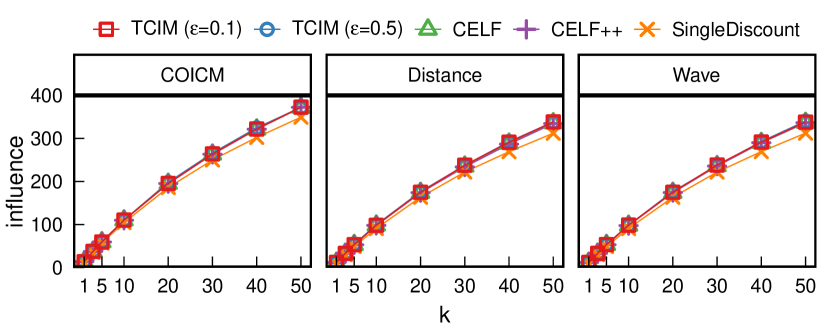
Figure 3: Results on the Facebook-like network: Influence versus $k$ under Campaign-Oblivious Independent Cascade Model (COCIM), Distance-based model and Wave propagation model. ($|S_{A}|=50$, $\ell=1$)

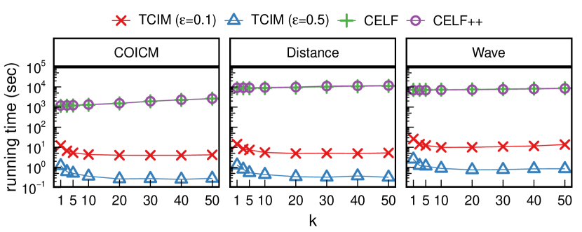
Figure 4: Results on the Facebook-like network: Running time versus $k$ under Campaign-Oblivious Independent Cascade Model (COCIM), Distance-based model and Wave propagation model. ($|S_{A}|=50$, $\ell=1$)

Results on large networks: For NetHEPT and Epinion, we experiment by varying $k$, $|S_{A}|$ and $\epsilon$ to demonstrate the efficiency and effectiveness of the TCIM. We compare the influence spread of TCIM to SingleDiscount heuristic only, since CELF and CELF++ do not scale well on larger datasets.

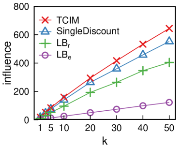
(a) NetHEPT

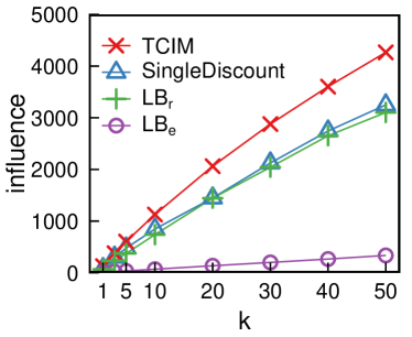
(b) Epinion

Figure 5: Results on large datasets: Influence spreads versus $k$ under the Wave propagation model. ($|S_{A}|\!=\!50$, $\epsilon\!=\!0.1$, $\ell\!=\!1$)

Figure 5 shows the influence spread of the solution returned by TCIM and SingleDiscount, where the influence propagation model is the Wave propagation model. We also show the value of $LB_{\text{e}}$ and $LB_{\text{r}}$ returned by the lower bound estimation and refinement algorithm. On both datasets, the expected influence of the seeds returned by TCIM exceeds the expected influence of the seeds return by SingleDiscount. Moreover, as in TIM/TIM⁺ [2], for every $k$, the lower bound $LB_{\text{r}}$ improved by Algorithm 3 is significant larger than the lower bound $LB_{\text{e}}$ returned by Algorithm 2. When the influence propagation model is COICM or the Distance-based model, the results are similar to that in Figure 5.

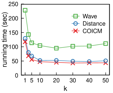
(a) NetHEPT

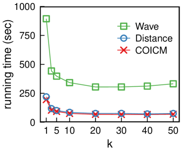
(b) Epinion

Figure 6: Results on large datasets: Running time versus $k$ under Campaign-Oblivious Independent Cascade Model (COCIM), Distance-based model and Wave propagation model. ($|S_{A}|=50$, $\epsilon=0.1$, $\ell=1$)

Figure 6 shows the running time of TCIM, with $k$ varying from $1$ to $50$. As in [2], for every influence propagation model, when $k\!=\!1$, the running time of TCIM is the largest. With the increase of $k$, the running time tends to drop first, and it may increase slowly after $k$ reaches a certain number. This is because the running time of TCIM is mainly related to the number of RAPG instances generated in Algorithm 1, which is $\theta=\lambda/LB_{\text{r}}$. When $k$ is small, $LB_{\text{r}}$ is also small as $OPT$ is small. With the increase of $k$, if $LB_{\text{r}}$ increases faster than the decrease of $\lambda$, $\theta$ decreases and the running time of TCIM also tends to decrease. From Figure 6, we see that TCIM is especially efficient when $k$ is large. Moreover, for every $k$, among three models, the running time of TCIM based on the Campaign-Obilivous Independent Cascade Model is the smallest while the running time of TCIM based on the Wave propagation model is the largest. This is consistent with the analysis of the running of TCIM in Section V.

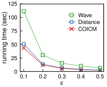
(a) NetHEPT

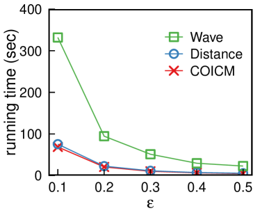
(b) Epinion

Figure 7: Results on large datasets: Running time versus $\epsilon$ under Campaign-Oblivious Independent Cascade Model (COCIM), Distance-based model and Wave propagation model. ($|S_{A}|=50$, $k=50$, $\ell=1$)

Figure 7 shows that the running time of TCIM decreases quickly with the increase of $\epsilon$, which is consistent with its $O(c(\ell+k)(m+n)\log n/\epsilon^{2})$ time complexity. When $\epsilon\!=\!0.5$, TCIM finishes within 7 seconds for NetHEPT dataset and finishes within 23 seconds for Epinion dataset. This implies that if we do not require a very tight approximation ratio, we could use a larger $\epsilon$ as input and the performance of TCIM could improve significantly.

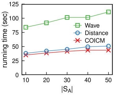
(a) NetHEPT

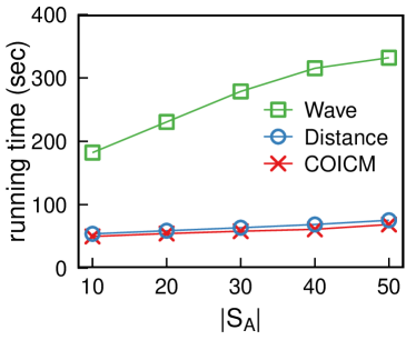
(b) Epinion

Figure 8: Results on large datasets: Running time versus $|S_{A}|$ under Campaign-Oblivious Independent Cascade Model (COCIM), Distance-based model and Wave propagation model. ($k=50$, $\epsilon=0.1$, $\ell=1$)

Figure 8 shows the running time of TCIM as a function of the seed-set size of source $A$. For any given influence propagation model, when $|S_{A}|$ increases, $OPT$ decreases and $LB_{\text{r}}$ tends to decrease. As a result, the total number of RAPG instances required in the node selection phase increases and consequently, the running time of TCIM also increases.

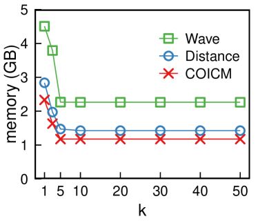
(a) NetHEPT

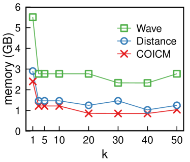
(b) Epinion

Figure 9: Results on large datasets: Memory consumption versus $k$ under Campaign-Oblivious Independent Cascade Model (COCIM), Distance-based model and Wave propagation model. ($|S_{A}|=50$, $\epsilon=0.1$, $\ell=1$)

Figure 9 shows the memory consumption of TCIM as a function of $k$. For any $k$, TCIM based on Campaign-Oblivious Independent Cascade Model consumes the least amount of memory because we only need to store the nodes for each RAPG instance. TCIM based on Wave propagation model consumes the largest amount of memory because we need to store both the nodes and edges of each RAPG instance. For the Distance-based model, we do not need to store the edges of RAPG instances, but need to store some other information for each RAPG instance; therefore, the memory consumption is in the middle. For all three propagation models and on both datasets, the memory requirement drops when $k$ increases because the number of RAPG instances required tends to decrease.

VIII Conclusion

In this work, we introduce a “General Competitive Independent Cascade (GCIC)” model and define the “Competitive Influence Maximization (CIM)” problem. We then present a Two-phase Competitive Influence Maximization (TCIM) framework to solve the CIM problem under GCIC model. TCIM returns $(1-1/e-\epsilon)$-approximate solutions with probability at least $1-n^{-\ell}$ and has time complexity $O(c(\ell+k)(m+n)\log n/\epsilon^{2})$, where $c$ depends on specific influence propagation model and may also depend on $k$ and graph $G$. To the best of our knowledge, this is the first general algorithmic framework for the Competitive Influence Maximization (CIM) problem with both performance guarantee and practical running time. We analyze TCIM under the Campaign-Oblivious Independent Cascade model in [6], the Distance-based model and the Wave propagation model in [4]. And we show that, under these three models, the value of $c$ is $O(1)$, $O(k)$ and $O(kn)$ respectively. We provide extensive experimental results to demonstrate the efficiency and effectiveness of TCIM. The experimental results show that TCIM returns solutions comparable with those returned by the previous state-of-the-art greedy algorithms, but it runs up to four orders of magnitute faster than them. In particular, when $k\!=\!50$, $\epsilon\!=\!0.1$ and $\ell\!=\!1$, given the set of $50$ nodes selected by the competitor, TCIM returns the solution within $6$ minutes for a dataset with $75,879$ nodes and $508,837$ directed edges.

References

• [1] D. Kempe, J. Kleinberg, and É. Tardos, “Maximizing the spread of influence through a social network,” in KDD.   ACM, 2003.
• [2] Y. Tang, X. Xiao, and Y. Shi, “Influence maximization: Near-optimal time complexity meets practical efficiency,” in SIGMOD.   ACM, 2014.
• [3] S. Bharathi, D. Kempe, and M. Salek, “Competitive influence maximization in social networks,” in Internet and Network Economics.   Springer, 2007.
• [4] T. Carnes, C. Nagarajan, S. M. Wild, and A. Van Zuylen, “Maximizing influence in a competitive social network: a follower’s perspective,” in ICEC.   ACM, 2007.
• [5] A. Borodin, Y. Filmus, and J. Oren, “Threshold models for competitive influence in social networks,” in Internet and network economics.   Springer, 2010.
• [6] C. Budak, D. Agrawal, and A. El Abbadi, “Limiting the spread of misinformation in social networks,” in WWW.   ACM, 2011.
• [7] J. Leskovec, A. Krause, C. Guestrin, C. Faloutsos, J. VanBriesen, and N. Glance, “Cost-effective outbreak detection in networks,” in ICDM.   ACM, 2007.
• [8] W. Chen, Y. Wang, and S. Yang, “Efficient influence maximization in social networks,” in KDD.   ACM, 2009.
• [9] W. Chen, C. Wang, and Y. Wang, “Scalable influence maximization for prevalent viral marketing in large-scale social networks,” in KDD.   ACM, 2010.
• [10] W. Chen, Y. Yuan, and L. Zhang, “Scalable influence maximization in social networks under the linear threshold model,” in ICDM.   IEEE, 2010.
• [11] A. Goyal, W. Lu, and L. V. Lakshmanan, “Celf++: optimizing the greedy algorithm for influence maximization in social networks,” in WWW.   ACM, 2011.
• [12] K. Jung, W. Heo, and W. Chen, “Irie: Scalable and robust influence maximization in social networks,” in ICDM.   IEEE Computer Society, 2012.
• [13] C. Borgs, M. Brautbar, J. Chayes, and B. Lucier, “Maximizing social influence in nearly optimal time,” in SODA, vol. 14.   SIAM, 2014.
• [14] J. Kostka, Y. A. Oswald, and R. Wattenhofer, “Word of mouth: Rumor dissemination in social networks,” in Structural Information and Communication Complexity.   Springer, 2008.
• [15] X. He, G. Song, W. Chen, and Q. Jiang, “Influence blocking maximization in social networks under the competitive linear threshold model.” in SDM.   SIAM, 2012.
• [16] G. L. Nemhauser, L. A. Wolsey, and M. L. Fisher, “An analysis of approximations for maximizing submodular set functions—i,” Mathematical Programming, vol. 14, no. 1, 1978.
• [17] T. Opsahl and P. Panzarasa, “Clustering in weighted networks,” Social networks, vol. 31, no. 2, 2009.
• [18] M. Richardson, R. Agrawal, and P. Domingos, “Trust management for the semantic web,” in The Semantic Web-ISWC 2003.   Springer, 2003.