Finite-size scaling at the first-order quantum transitions of quantum Potts chains

Abstract

We investigate finite-size effects in quantum systems at first-order quantum transitions. For this purpose we consider the one-dimensional $q$-state Potts models which undergo a first-order quantum transition for any $q>4$, separating the quantum disordered and ordered phases with a discontinuity in the energy density of the ground state. The low-energy properties around the transition show finite-size scaling, described by general scaling ansatzes with respect to appropriate scaling variables. The size dependence of the scaling variables presents a particular sensitiveness to boundary conditions, which may be considered as a peculiar feature of first-order quantum transitions.

I Introduction

Zero-temperature quantum phase transitions Sachdev-book ; Vojta-03 arise in many-body systems with competing ground states controlled by nonthermal model parameters. They are of first order when the infinite-volume ground-state properties are discontinuous across the transition point. First-order quantum transitions (FOQTs) are of great interest, as they occur in a large number of quantum many-body systems, such as quantum Hall samples PPBWJ-99 , itinerant ferromagnets VBKN-99 , heavy fermion metals UPH-04 ; Pfleiderer-05 ; KRLF-09 , etc.

Although FOQTs do not develop a diverging correlation length in the infinite-volume limit, they show finite-size scaling (FSS) behaviors around the transition point, which turn out to be particularly sensitive to the boundary conditions CNPV-14 . Indeed, unlike FSS at continuous transitions, the size dependence of the FOQT scaling variables may significantly change when varying the boundary conditions. For example, in the case of the FOQTs of Ising chains, driven by a magnetic field in their quantum ferromagnetic phase, we have an exponential size dependence for open and periodic boundary conditions, while it is power law for antiperiodic or kink-like boundary conditions. Actually, this particular sensitiveness to the boundary conditions may be considered as a peculiar feature of FOQTs, which qualitatively distinguishes their FSS behaviors from those at continuous quantum transitions SGCS-97 ; CPV-14 . An understanding of these finite-size properties is important for a correct interpretation of experimental or numerical data when quantum phase transitions are investigated in relatively small systems.

In Ref. CNPV-14 we put forward general ansatzes for the FSS at a FOQT driven by a generic parameter $g$. Around the FOQT point $g_{c}$, the relevant scaling variable $\kappa$ is expected to be the ratio between the energy contribution $E_{L}$ of the perturbation driving the transition [generally $E_{L}\approx(g-g_{c})L^{\zeta}$ where $\zeta$ is an appropriate exponent] and the energy difference (gap) of the lowest states $\Delta_{L}\equiv E_{1}-E_{0}$ at $g=g_{c}$. Then, around $g_{c}$, the gap satisfies the FSS ansatz

$$\Delta(L,g)\equiv E_{1}(L,g)-E_{0}(L,g)\approx\Delta_{L}f_{\Delta}(\kappa),$$ (1)

where $\Delta_{L}\equiv\Delta(L,g_{c})$, thus $f_{\Delta}(0)=1$. Analogous scaling behaviors apply to other quantities. For example, the magnetization is expected to asymptotically behave as

$$m(L,g)\approx m_{0}f_{m}(\kappa),$$ (2)

where $m_{0}$ is a normalization which we identify with the magnetization obtained approaching the transition point $g\to g_{c}$ from the ordered phase, after the infinite-volume limit. The above FSS ansatzes represent the simplest scaling behaviors compatible with the FOQT discontinuities arising in the infinite-volume limit. The ansatzes can also be extended to allow for the temperature CNPV-14 . The particular sensitiveness to the boundary conditions essentially arises from the energy gap at $g_{c}$ entering the scaling variable $\kappa$, whose finite-size behavior depends crucially on the boundary conditions considered. Hence, once the scaling variables are expressed in terms of the parameter driving the transition and the size $L$, the $L$ dependence of the FSS may significantly change according to the chosen boundary conditions. The above scaling ansatzes have been checked, and confirmed, at the FOQT of Ising chains in the ferromagnetic phase, driven by the (odd) magnetic field coupled to the order-parameter spin operator. CNPV-14

In this paper we further develop this issue, extending the FSS analysis to FOQTs driven by (even) temperature-like parameters, with a discontinuity in the infinite-volume energy density of the ground state. For this purpose we consider the quantum $q$-state Potts chains SP-81 ; IS-83 , which undergo FOQTs for a sufficiently large number of states, i.e. $q>4$ Baxter-73 ; Wu-82 . They provide a theoretical laboratory to test the scaling arguments at FOQTs in a controlled framework, due to the relative simplicity of the model for which the transition point is exactly known. We observe FSS described by the general ansatzes (1) and (2). Moreover, like FOQTs of the Ising chains CNPV-14 , its asymptotic size dependence turns out to be particularly sensitive to the choice of the boundary conditions, giving rise to size dependences with different power laws.

The paper is organized as follows. In Sec. II we present the quantum $q$-state Potts models, and discuss the boundary conditions of finite chains. In Sec. III we introduce some relevant observables, and discuss their behavior at the FOQTs for $q>4$. In Sec. IV we present a numerical analysis around the transition point, which supports the general FSS ansatzes at FOQTs. In Sec. V we discuss the FSS behaviors at the FOQTs driven by parallel magnetic fields in the ordered ferromagnetic phase, which resemble those for Ising chains. Finally, we draw some conclusions in Sec. VI. A few appendices report some details on the duality property of the quantum Potts chains, and the numerical methods used to study them, which are based on the density-matrix renormalization-group (DMRG) techniques Sch-05 .

II The quantum Potts chain

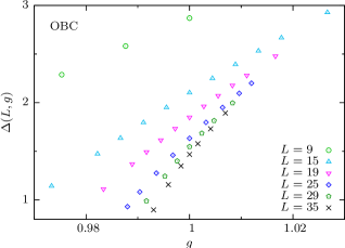
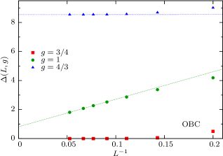
Figure 1: (Top) The gap $\Delta(L,g)$ for the $q=10$ Potts chain with OBC, around $g=1$ and for several values of $L$. (Bottom) $\Delta_{L}(L,g)$ vs $1/L$ at the transition point $g=1$, in the disordered ($g=4/3$) and ordered ($g=3/4$) phases. The dotted lines are a linear fits of the data for the largest chains.

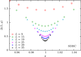
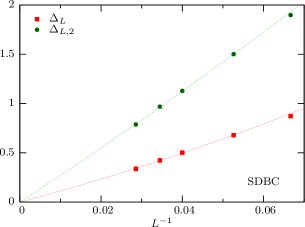
Figure 2: Energy differences of the lowest states for the $q=10$ Potts chain with SDBC. The bottom figure shows data at $g=g_{c}$, for $\Delta_{L}\equiv E_{1}-E_{0}$ and $\Delta_{L,2}\equiv E_{2}-E_{0}$, providing evidence for an asymptotic $O(L^{-1})$ power-law behavior. The dotted lines are drawn to guide the eyes (they show fits to $p(L)=b_{1}/L+b_{2}/L^{2}$ of the data for $L>15$). The top figure shows data for the gap $\Delta(L,g)$ around the transition point for several values of $L$.

The quantum one-dimensional (1D) Potts chain is the quantum analog of the classical 2D Potts model Potts-52 ; Wu-82

$$H_{c}=-J\sum_{\langle ij\rangle}\delta(s_{i},s_{j}),$$ (3)

where the sum is over the nearest-neighbor sites of a square lattice, $s_{i}$ are spin variables taking $q$ integer values, i.e. $s_{i}=1,...,q$, and $\delta(m,n)=1$ if $m=n$ and zero otherwise. A corresponding 1D quantum Hamiltonian is derived from the time continuum limit of the transfer matrix SP-81 . The quantum $q$-state Potts chain involves $q$ states per site, which can be labeled by an integer number $|n=1\rangle,...,|n=q\rangle$. The Hamiltonian of a chain of $L$ sites can be written as SP-81 ; IS-83

$$H=-J_{q}\sum_{j=1}^{L-1}\sum_{k=1}^{q-1}\Omega_{j}^{k}\Omega_{j+1}^{q-k}-g\sum_{j=1}^{L}\sum_{k=1}^{q-1}M_{j}^{k}$$ (4)

where $J_{q}\equiv J/q$, $\Omega_{j}$ and $M_{j}$ are $q\times q$ matrices:

$$\Omega=\delta_{m,n}\,\omega^{n-1},\qquad\omega=e^{i2\pi/q},$$ (5)

$$M=\delta_{m,{\rm Mod}(n-1,q)}=\begin{pmatrix}0&1&&\\ &\ddots&\ddots&\\ &&&1\\ 1&&&0\\ \end{pmatrix}.$$ (6)

These matrices commute on different sites and satisfy the algebra: SP-81 $\Omega_{j}^{k}\Omega_{j}^{l}=\Omega_{j}^{k+l}$, $M_{j}^{k}M_{j}^{l}=M_{j}^{k+l}$, $\Omega_{j}^{q}=M_{j}^{q}=\mathbb{I}$, $M_{j}^{k}\Omega_{j}^{l}=\omega^{kl}\Omega_{j}^{l}M_{i}^{k}$. For $q=2$ we recover the quantum Ising chain.

Like Ising chains, the ground state of model (4) have two phases: a disordered phase for sufficiently large values of $g$ and an ordered phase for small $g$ where the system magnetizes along one of the $q$ directions. Indeed, for $g\to 0$ the ground state (without further external fields) is degenerate, given by the $q$ states $\prod_{j}|n\rangle_{j}$, while for $g\to\infty$ it is nondegenerate and given by $\prod_{j}\sum_{n=1}^{q}|n\rangle_{j}$.

Like Ising chains, quantum Potts chains satisfy a self-duality property SP-81 , i.e.

$$H(g/J_{q})=(g/J_{q})H(J_{q}/g),$$ (7)

see also App. A. Therefore the transition point $g_{c}$ separating the two phases must be located at $g_{c}=J_{q}$. The phase transition is discontinuous (first order) for $q>4$ Baxter-73 ; Wu-82 . It becomes stronger and stronger with increasing $q$, i.e. the infinite-volume discontinuities increase with increasing $q$.

The boundary conditions that we consider in our FSS study are specific cases of the boundary Hamiltonian

$$H_{b}=-J_{q}\left[h_{1}\sum_{k=1}^{q-1}\Omega_{1}^{k}+h_{L}\sum_{k=1}^{q-1}\Omega_{L}^{k}\right],$$ (8)

which is added to the bulk Hamiltonian (4). The value $h_{1}=1$ (or $h_{L}=1$) is equivalent to having a further fictitious site at $i=0$ (or $i=L+1$) with a fixed state $|n=1\rangle$. On the other hand, the value $h_{1}=0$ (or $h_{L}=0$) is equivalent to having a further site $i=0$ (or $i=L+1$) with an disordered unmagnetized state $\propto\sum_{n}|n\rangle$. Therefore, the case $h_{1}=h_{L}=1$ corresponds to fixed parallel boundary conditions (FPBC) favoring the ordered phase, and the case $h_{1}=h_{L}=0$ to open boundary conditions (OBC) favoring the disordered phase.

Self duality (7) is violated by finite chains with generic boundary conditions, and in particular for generic values of $h_{1},\,h_{L}$. However, there is a notable exception, when $h_{1}=1$ and $h_{L}=0$ (or viceversa), corresponding to mixed boundary conditions, fixed and open at the two extremes (self-duality also requires a spacial inversion $i\to L-i$), see App. A. Thus the duality relation (7), and in particular the relation for the eigenspectrum

$$E_{n}(L,g/J_{q})=(g/J_{q})E_{n}(L,J_{q}/g),$$ (9)

is satisfied for any finite chain when using these self-dual boundary conditions (SDBC).

We define the magnetization of the ground state as

$$m(L,g,x)=\langle{\cal M}_{x}\rangle,$$ (10)

$${\cal M}_{x}={q\delta(n_{x},1)-1\over q-1},\quad\delta(n_{x},1)={1\over q}\sum_{k=1}^{q}\Omega_{x}^{k},$$ (11)

such that $m=1$ if the site $x$ is along $n=1$, and $m=0$ if the state at $x$ is an equally probable superposition of $q$ states. The magnetization provides an order parameter: indeed it vanishes in the disorder phase ($g>1$) and jumps discontinuously at the FOQT to a nonzero value in the ordered phase, for $q>4$. In particular,

$$m_{0}={\rm lim}_{g\to 1^{-}}\;{\rm lim}_{h\to 0}\;{\rm lim}_{L\to\infty}\;m(L,g,x)$$ (12)

is non zero for $q>4$, where $h$ is a global magnetic field coupled to the magnetization operator, e.g. described by the Hamiltonian term $H_{h}=-h\sum_{j}\sum_{k=1}^{q}\Omega_{j}^{k}$.

The infinite-volume energy density of the ground state changes discontinuously across the FOQT. We consider the definition

$$e(L,g,x)=\langle{\cal E}_{x}\rangle,$$ (13)

$${\cal E}_{x}=\delta(n_{x},n_{x+1})={1\over q}\sum_{k=1}^{q}\Omega_{x}^{k}\Omega_{x+1}^{q-k}.$$

The FOQT limits

$$e_{\pm}={\rm lim}_{g\to 1^{\pm}}\;{\rm lim}_{L\to\infty}\;e(L,g,x)$$ (14)

differ at the FOQTs of the Potts chains with $q>4$. Their difference $\Delta e\equiv e_{+}-e_{-}$ is the analog of the latent heat of first-order classical transitions.

In the following we set $J_{q}=1$, thus the Hamiltonian depends on the parameter $g$ only, and $g_{c}=1$.

III Size dependence at the transition point

In this section and next one we present a numerical analysis of the $q=10$ Potts chains, employing DMRG techniques Sch-05 . Some details on the implementation of DMRG methods for Potts chains are reported in App. B.

To begin with, we report the estimates of the infinite-volume magnetization and energy values at the transition point, cf. Eqs. (12) and (14), which characterize the discontinuities of the ground state at the FOQT in the infinite-volume limit. Infinite-size extrapolations of DMRG calculations at $g=1$ with FPBC and OBC, favoring respectively the ordered and disordered phases, provide the $q=10$ estimates

$$m_{0}=0.8572(1),\;e_{-}=0.8060(1),\;e_{+}=0.3745(5).$$ (15)

At the transition point $g_{c}=1$ for $q>4$, when the Potts chain undergoes a FOQT, the energy difference (gap) of the lowest states turns out to significantly depend on the choice of the boundary conditions.

Let first consider OBC, which do not break the permutation symmetry of the model. Fig. 1 reports some numerical results for the energy difference of the lowest states of the $q=10$ Potts chain. The data show that the energy difference of the lowest states approaches a nonzero constant value in the disordered phase ($g>1$), i.e.

$$\Delta(L,g>1)=D(g)+O(L^{-1}).$$ (16)

This behavior is also observed at the transition point $g=1$, due to the fact that OBC favors disordered state. Then, in the ordered phase ($g<1$) the ground state tends to be degenerate, and the gap gets exponentially suppressed, see also Sec V. As shown in Fig. 1 the gap drops for $g\lesssim 1$, in a region of size $O(L^{-1})$ close to $g=1$, see also Ref. IS-83 . The gap at $g=1$ approaches a constant also in the case of FPBC, which favors the ordered phase.

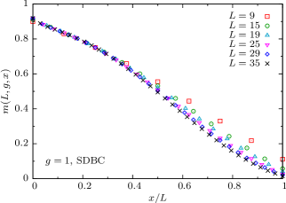
Figure 3: Space dependence of the magnetization (10) of the $q=10$ Potts chain with SDBC at the FOQT point $g=1$. The data versus $x/L$ approach a scaling curve with increasing $L$.

A different behavior is found for SDBC. In this case the gap satisfies the duality relation

$$\Delta(L,g)=g\Delta(L,1/g),$$ (17)

which is a trivial consequence of Eq. (9). Some results for $q=10$ are shown in Fig. 2. The energy differences of the lowest states at $g=g_{c}$ turn out to approximately decrease as $1/L$ with increasing $L$, while they approach nonzero values for both $g>1$ and $g<1$, in agreement with Eq. (17). More precisely, the data of $\Delta_{L}\equiv\Delta_{L,1}$ and $\Delta_{L,2}$, related to the first and second excited state respectively, fit the behavior

$$\Delta_{L,k}\equiv\Delta_{k}(L,g=g_{c})={c_{k}\over L}+{c_{k2}\over L^{2}}+....$$ (18)

Although the data clearly distinguish the $O(L^{-1})$ asymptotic behavior from other power laws, such as $O(L^{0})$ or $O(L^{-2})$, see Fig. 2, they are not sufficient to obtain accurate estimates of the coefficients $c_{i}$. Some rough estimates are $c_{1}\approx 9$ and $c_{2}\approx 3c_{1}$ for $q=10$.

Analogous results are expected at the FOQTs for other values of $q>4$. Once again, these results demonstrate how the size dependence significantly changes when different boundary conditions are considered at FOQTs.

We mention that some earlier analyses on the finite-size dependence at the FOQTs of Potts chain appeared in Refs. IS-83 ; IC-99 , focussing essentially on the large-$q$ limit. Actually the $O(L^{-1})$ finite-size behavior (18) of the gap appears to contradict the large-$q$ results of Ref. IC-99 , obtaining $\Delta_{L}\sim 1/L^{2}$ for the same SDBC. However, they were obtained by first taking the $q\to\infty$ limit and then the large-$L$ limit. This order of the limits does not necessarily reproduce the correct results for the finite-size scaling at finite $q$, even at large $q$, because the large-$q$ limit should be taken after the large-$L$ limit.

The magnetization (10) vanishes for OBC due to the $q$-state permutation symmetry. It is nonzero for SDBC which explicitly (softly) breaks the $q$-state symmetry at one of the boundaries. Fig. 3 shows its space dependence at the transition point of the $q=10$ Potts chain with SDBC: it goes from a number close to one at the fixed $|n=1\rangle$ boundary to a number close to zero at the opposite open extremity. Actually the data of the local magnetization $m(L,1,L)$ at the open extremity appears to vanish, apparently as $L^{-2}$. Note that with increasing $L$ the data scale as

$$m(L,g=1,x)\approx F(x/L).$$ (19)

IV Finite-size scaling at the FOQT

First-order classical transitions, driven by thermal fluctuations, show FSS behaviors analogous to those observed at continuous transitions FB-72 ; Barber-83 ; Cardy-fss ; Privman-90 ; PHA-91 ; PV-02 , with appropriate critical exponents related to the spatial dimensionality $d$ of the system, see e.g. Refs. NN-75 ; FB-82 ; PF-83 ; FP-85 ; CLB-86 ; LK-91 ; BK-92 ; BNB-93 ; VRSB-93 ; CPPV-04 ; BDV-14 . The extension of FSS to FOQTs is already expected on the basis of the general quantum-to-classical mapping of $d$-dimensional quantum systems into classical $(d+1)$-dimensional systems with anisotropic slab-like geometry. Indeed, a universal FSS behavior emerges also at FOQTs CNPV-14 . However, unlike FSS at continuous transitions, the depencence of the scaling variables on the size $L$ may change significantly. For example, at the FOQTs of Ising chains driven by a parallel magnetic field in their ordered phase, the scaling variables are related to the size $L$ by exponential or power laws, depending on the properties of the low-energy spectrum for the given boundary conditions. In the case of the FOQTs of Ising chains, this particular sensitiveness of the gap to the boundary conditions was also noted in Refs. CJ-87 ; LMMS-12 .

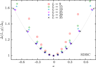
Figure 4: FSS of the gap for the $q=10$ Potts chain with SDBC: we plot the ratio $\Delta(L,g)/\Delta_{L}$ versus $\kappa=(g-1)L/\Delta_{L}$ for several values of $L$. They appear to approach an asymptotic FSS curve with increasing $L$. The raw data were already shown in Fig. 2. The dotted line shows the optimal fit of the data of the largest lattice to the function $\sqrt{1+c\,\kappa^{2}}$ with $c\approx 2.7$.

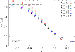
Figure 5: FSS of the central-site magnetization (22) for the $q=10$ Potts chain with SDBC. The data are consistent with an asymptotic FSS as predicted by Eq. (2). The dashed line indicates the inifinite-volume magnetization value, cf. Eq. (15).

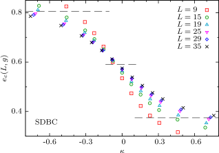
Figure 6: FSS of the energy density $e_{c}(L,g)$ at the center of the chain, cf. Eq. (13), for the $q=10$ Potts chain with SDBC. The data approach a scaling function of $\kappa\equiv(g-1)L/\Delta_{L}$. They are consistent with the asymptotic behaviors given by the values $e_{\pm}$, cf. Eq. (15), which are indicated by the dashed lines. At $g=g_{c}$, i.e. $\kappa=0$, the data approach the average value $(e_{+}+e_{-})/2\approx 0.590$ (dashed line around $\kappa=0$).

We now check the FSS scenario at the FOQTs of the $q=10$ Potts chain by analyzing the numerical DMRG data of the energy differences of the lowest states, the magnetization and energy density of the ground state.

According to the general arguments outlined in Sec. I, the relevant scaling variable is expected to be

$$\kappa={(g-1)L/\Delta_{L}},$$ (20)

i.e. the ratio between $E_{L}\sim(g-1)L$, the energy contribution of the perturbation driving the FOQT, and the gap $\Delta_{L}$ at the FOQT point.

We first consider the model with SDBC, whose gap decays as $1/L$ at the transition point. Fig. 4 shows that the data for the ratio $\Delta(L,g)/\Delta_{L}$ approach a nontrivial scaling curve in the large-$L$ limit when they are plotted versus the scaling variable $\kappa$, nicely supporting the scaling ansatz (1). Note that the scaling function $f_{\Delta}(\kappa)$ must be an even function of $\kappa$ due to the duality relation (17). Since the disordered phase is generally gapped, duality also implies that $f_{\Delta}(\kappa)\to\infty$ for $\kappa\to\pm\infty$. Actually the data for the largest lattices suggest that

$$f_{\Delta}(\kappa)=\sqrt{1+c\,\kappa^{2}},$$ (21)

which is the simplest even function which diverges as $|\kappa|$, matching the expected linear large-$L$ increase of the gap for finite differences $g-1>0$.

The scaling behavior of the magnetization $m_{c}(L,g)$ at the center of the chain,

$$m_{c}(L,g)\equiv m(L,g,x_{c}),$$ (22)

(with $x_{c}=(L+1)/2$ for chains with an odd number of sizes) is shown In Fig. 5. The plot of the data versus $\kappa$ definitely supports the scaling behavior (2). Asymptotically for $\kappa\to-\infty$, the FSS curve appears to converge toward the value $m_{0}$ defined in Eq. (12), thus $f_{m}(\kappa)\to 1$ for $\kappa\to-\infty$ and $f_{m}(\kappa)\to 0$ for $\kappa\to\infty$.

Evidence of the FSS is also provided by the data of the energy density $e_{c}(L,g)\equiv e(L,g,x_{c})$ at the center of the chain, cf. Eq. (13), see Fig. 6. These data appear to converge toward a scaling curve which has the values $e_{\pm}$, cf. Eq. (14), as asymptotics. Therefore, they suggest the scaling behavior

$$e_{c}(L,g)\approx f_{e}(\kappa)$$ (23)

with $f_{e}(\pm\infty)=e_{\pm}$ and $f(0)=(e_{+}+e_{-})/2$.

Scaling behaviors are also observed in the case of OBC. In this case the magnetization vanishes by symmetry. The results in Fig. 7 show a good evidence of the FSS ansatz (1) for the energy difference of the lowest states. However, we stress that the actual size dependence of the FSS is quite different from the case of SDBC where $\Delta_{L}=c/L+O(L^{-2})$, because $\Delta_{L}={\rm cost}+O(L^{-1})$ for OBC. Also the data of the energy density at the center of the chain show evidence of scaling with respect to the variable $\kappa$, in agreement with Eq. (13).

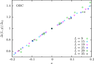
Figure 7: FSS of the gap for the $q=10$ Potts chain with OBC. The data approach a FSS curve with increasing the size $L$.

We expect that analogous results hold at the FOQTs for any $q>4$. However, the values of $L$ where the asymptotic behavior begins being observed may vary. We expect that larger sizes are necessary for weaker FOQTs, i.e. smaller $q$, and smaller for stronger FOQTs, i.e. larger $q$ values.

V FOQT driven by a magnetic field in the ferromagnetic phase

We now consider the FOQTs which occur in the ferromagnetic phase, i.e. when $g<1$, driven by a parallel magnetic field along one of the $q$ directions, $n=1$ say. In other words, we now consider a Potts chain described by adding a magnetic term coupled to the global operator $\sum_{j}\delta(n_{j},1)$, i.e.

$$H_{f}=H-h\sum_{j=1}^{L}\sum_{k=1}^{q}\Omega_{j}^{k}$$ (24)

where we use Eq. (11). We consider OBC which do not break the $q$-state permutation symmetry. We study the interplay between the finite size and the magnetic field $h$. For any value of $q$, thus including the Ising chain for $q=2$, the system has a line of FOQTs in the ordered ferromagnetic phase, i.e. $g<1$, driven by the magnetic field $h$, which breaks the $q$-state permutation symmetry, giving rise to a discontinuity of the magnetization (10).

The finite-size behavior at these FOQTs in the quantum Ising chain, i.e. the Hamiltonian (24) for $q=2$, is analyzed in Ref. CNPV-14 , confirming the general FSS ansatzes (1) and (2). In the Ising case with boundary conditions which do not break the Z₂ symmetry, such as OBC, the two states with up and down global magnetization become degenerate for $L\to\infty$. In finite systems, an exponentially suppressed matrix element between these states solve the degeneracy by mixing them, giving rise to a phenomenon of avoided level crossings in many-body systems. Thus the scaling functions can be determined exactly by considering the theory restricted to the subspace spanned by the two lowest-energy states. Here we extend these computations to higher values of $q$.

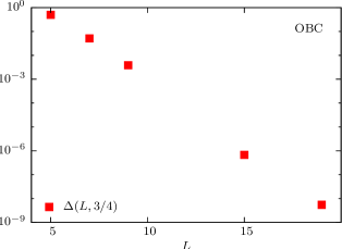
Figure 8: The gap of the $q=10$ Potts chain for $g=3/4$ and $h=0$, with OBC. The data show an exponential suppression with increasing $L$.

In the infinite-size limit without symmetry breaking terms, i.e. for $h=0$, the low-energy energy spectrum of the ferromagnetic phase is characterized by a degeneracy of the $q$ states $|\psi_{n}\rangle\equiv\prod_{j}|n\rangle_{j}$ with $n=1,...,q$. In a finite system, the presence of a nonvanishing matrix element among these states, essentially due to tunneling effects, lifts the degeneracy. The energy difference $\Delta_{L,k}$ of the lowest states for $h=0$ vanishes exponentially as $L$ increases, see, e.g., Fig. 8, roughly as $\Delta_{L}\sim e^{-cL}$. According to the general scaling arguments outlined in Sec. I, the scaling variable to describe the FSS at these FOQTs is expected to be

$$\kappa\sim hL/\Delta_{L}.$$ (25)

Therefore the size dependence of $\kappa$ is exponential in this case, i.e. $\kappa\sim hLe^{cL}$, analogously to the Ising $q=2$ case CNPV-14 .

Since the energy differences $\Delta_{L,k}$ of the lowest $q-1$ excited states with the ground state are exponentially suppressed in the large-$L$ limit, they are expected to be much smaller than the energy differences between the higher excited states and the ground state, i.e.

$$\Delta_{L,k\leq q-1}\ll\Delta_{L,k\geq q}.$$ (26)

Thus, we assume that, for sufficiently large $L$, the low-energy properties in the crossover region around $h=0$, and for sufficiently small $|h|$, are simply obtained by restricting the theory to the $q$ lowest-energy states $|n\rangle$. The Hamiltonian restricted to this subspace is a $q\times q$ matrix with the general form

$$H_{r}=\left(\begin{array}[]{l@{\ \ }l@{\ \ }l@{\ \ }l@{\ \ }l}\varepsilon-\beta&\quad-\delta&\quad...&\quad-\delta\\ -\delta&\quad\varepsilon+{\beta\over q-1}&\quad...&\quad-\delta\\ ...&\quad...&\quad...&\quad...\\ -\delta&\quad-\delta&\quad...&\quad\varepsilon+{\beta\over q-1}\\ \end{array}\right)\;$$ (31)

where we take into account that the system must satisfy the $q$-state permutation symmetry when $\beta=0$. $\beta\sim hL$ represents the perturbation induced by the magnetic field $h$. $\delta\geq 0$ is a small parameter which should vanish for $L\to\infty$ and $h=0$, in order to obtain a degenerate ground state; its sign is such to have the most symmetric state as ground state when $\beta=0$, as expected in ferromagnetic models.

The gap can be easily obtained by diagonalizing $H_{r}$, taking the differences of the eigevalues. In particular, for $q=3$ and setting $w=\beta/(3\delta)$, we obtain the energy differences

$${E_{1}-E_{0}\over 3\delta}=\sqrt{1-w+{9\over 4}w^{2}},$$ (32)

$${E_{2}-E_{0}\over 3\delta}={1\over 2}+{3\over 4}w+{1\over 2}\sqrt{1-w+{9\over 4}w^{2}},$$ (33)

where $E_{0}$ is the lowest egenvalue. These functions are shown in Fig. 9. The above expressions agree with the scaling ansatz (1) provided that we identify

$$3\delta\to\Delta_{L},\qquad w\to\kappa.$$ (34)

The scaling function $f_{\Delta}$ entering Eq. (1) can be easily derived from the r.h.s. of Eqs. (32) and (33), taking their lowest value. Analogous expressions can be straightforwardly obtained for higher $q$ values, although they turn out to be more cumbersome.

The ground-state magnetization can be obtained by computing the expectation value of

$${\cal M}={q\delta(n,1)-1\over q-1}$$ (35)

on the lowest eigenstate. In particular for $q=3$ the scaling function in Eq. (2) reads

$$f_{m}(\kappa)={\left({3\over 2}\sqrt{1-\kappa+{9\over 4}\kappa^{2}}-{1\over 2}+{9\over 4}\kappa\right)^{2}-1\over\left({3\over 2}\sqrt{1-\kappa+{9\over 4}\kappa^{2}}-{1\over 2}+{9\over 4}\kappa\right)^{2}+2}$$ (36)

This function is shown in Fig. 9. The above FSS functions are supposed to be asymptotically exact, i.e. for $L\to\infty$ keeping $\kappa$ fixed. They are also expected to be universal with respect to the values of the parameter $g<1$, which only enters through trivial normalizations of the scaling variables and functions. Scaling corrections are expected to be suppressed in the FSS limit, by powers of the inverse size. Boundary effects in the case of OBC are expected to be negligible for sufficiently large sizes.

The above $q$-level approximation provides also a framework to study the unitary quantum dynamics when $h$ varies (in time) in a small interval around $h=0$. Since only the $q$ lowest-energy states are relevant, the dynamics is a straightforward extension of that governing a two-level quantum mechanical system in which the energy separation of the two levels is a function of time (Landau-Zener effect  LZeff ).

Figure 9: The r.h.s. of Eqs. (32) and (33), and the scaling function of the magnetization (36).

In conclusion the above analysis based on a $q$-level approximation, restricting the Hamiltonian to the lowest almost-degenerate levels, confirms the general features of the FSS scenario at FOQTs in ferromagnetic phases driven by magnetic fields, generalizing the results of Ref. CNPV-14, for the Ising chains (corresponding to the $q=2$ case).

VI Conclusions

This paper continues the study of the finite-size scaling phenomena at FOQTs. We extend the checks of the general FSS ansatzes put forward in Ref. CNPV-14 , considering FOQTs driven by an even temperature-like parameter with a discontinuity in the ground-state energy density. For this purpose we consider the quantum $q$-state Potts chains which undergo a FOQT when $q>4$, separating quantum disordered and ordered phases. We present an extended numerical analysis of the $q=10$ case, based on DMRG computations, considering different boundary conditions: in particular OBC and SDBC, see Sec. II.

Our analysis of the finite-size dependence of various low-energy observables (such as the energy differences of the lowest states, the magnetization and the energy density of the ground state) provide evidence of asymptotic FSS behaviors for the various boundary conditions considered, as predicted by the general arguments leading to Eqs. (1), (2), and (23). However, this fact does not prevent the system from having different functional dependences on the finite size. Indeed, the actual size dependence is essentially due to the size dependence of the scaling variable $\kappa$, cf. Eq. (20), and in particular of the gap $\Delta_{L}$ entering its definition. This leads to different power laws when passing from open to mixed self-dual boundary conditions. The general sensitiveness of the FSS at FOQTs may be considered as their peculiar feature with respect to continuous quantum transitions.

We also discuss the FSS behavior at the FOQTs driven by parallel magnetic fields in the ordered ferromagnetic phase, for any $q$, thus also for the Ising chain. We argue that the FSS behavior can be obtained by extending the two-level approximation used in the case of Ising chains CNPV-14 , to a $q$-level approximation. Like the analogous FOQTs of Ising chains, we confirm the existence of FSS, with a scaling variable which depends exponentially on the size of the chain.

We stress that the FSS behavior at FOQTs is observed for relatively small sizes. Indeed, chains of size up to a few tens turn out to be sufficient to show the asymptotic FSS behavior. Thus, even small systems may show definite signatures of FOQTs, as also argued in Refs. CNPV-14 ; IZ-04 ; LMD-11 . This makes FSS at FOQTs particularly interesting, because it may require only modest-size systems to be observed. For this reason, the present results may be relevant for quantum simulators, where controllable quantum systems, usually of modest size, are engineered to reproduce particular Hamiltonians GAN-14 ; Islam-etal-11 ; Simon-etal-11 ; LMD-11 . Furthermore, in quantum computing, some algorithms, notably the adiabatic ones, rely on a sufficiently large gap Bloch-08 ; YKS-10 ; AC-09 ; LMMS-12 , and thus fail at FOQTs. The scaling theory that we present may help to understand how this occurs in finite systems.

We finally mention that an interesting extension of this study concerns the effects of inhomogeneous conditions at FOQTs, such as those induced by space dependent external fields. Nontrivial scaling phenomena emerge also in this case, with respect to the length scale of the induced inhomogeneity, in the space transition region between the two phases CNPV-15 .

Appendix A Self duality of quantum Potts chains

We first consider the finite-chain Potts model defined by the Hamiltonian

$$H_{\rm sd}=-J_{q}\sum_{j=1}^{L-1}\sum_{k=1}^{q-1}\Omega_{j}^{k}\Omega_{j+1}^{q-k}-g\sum_{j=1}^{L-1}\sum_{k=1}^{q-1}M_{j}^{k}$$ (37)

Notice that the difference with the Hamiltonian (4) is just relegated to the second sum which does not contain the lattice size $i=L$. In this case one can define an exact duality transformation, which maintains the form of the Hamiltonian (37), interchanging the role of the two sums, thus $J_{q}\to g$ and $g\to J_{q}$. This is achieved by defining the new operators $\widetilde{M}_{l}$ and $\widetilde{\Omega}_{l}$, SP-81 formally located between two adjacent sites, such that

$$\widetilde{M}_{j+1/2}^{k}=\Omega_{j}^{k}\Omega_{j+1}^{q-k},\qquad\widetilde{\Omega}_{j+1/2}^{k}=\prod_{i\leq j}M_{i}^{q-k},$$ (38)

which satisfy the same algebra of the original operators $\Omega_{j}$ and $M_{j}$. The inverse dual transformation reads

$$M_{l+1/2}^{k}=\widetilde{\Omega}_{l}^{k}\widetilde{\Omega}_{l+1}^{q-k},\qquad\Omega_{l-1/2}^{k}=\prod_{i\geq l}\widetilde{M}_{i}^{q-k}.$$ (39)

Note that, in order to get an Hamiltonian formally identical to $H_{\rm sd}$, one should also perform a space inversion $j\to L-j$. This duality properties imply that a unitary transformation $U$ exists such that

$$UH_{\rm sd}(J_{q},g)U^{\dagger}=H_{\rm sd}(g,J_{q})=gH_{\rm sd}(1,J_{q}/g),$$ (40)

which also implies the spectrum relation (9) for $J_{q}=1$.

Since $[\Omega_{L},H_{\rm sd}]=0$, the spectrum of $H_{\rm sd}$ is degenerate, with a degeneracy associated with the $q$ eigenstates of $\Omega_{L}$. This implies that the Hilbert space can be decomposed into $q$ subspaces ${\cal H}_{n}$, such that $\Omega_{L}\psi_{n}=\omega^{n-1}\psi_{n}$, cf. Eq. (5). If we restrict $H_{\rm sd}$ to ${\cal H}_{n=1}$, we obtain the model described by the Hamiltonian (4) supplemented with the boundary term (8) with $h_{1}=1$ and $h_{L}=0$, for a chain of length $L-1$. This is already sufficient to show that the finite Potts chain with SDBC is self dual, thus its spectrum satisfies the duality relation (9). Of course, this could have been demonstrated by directly using the duality transformations (beside those given in Eq. (38) one should use $\widetilde{M}_{L}^{k}=\Omega_{L}^{q-k}$).

Appendix B DMRG computations of the Potts chains

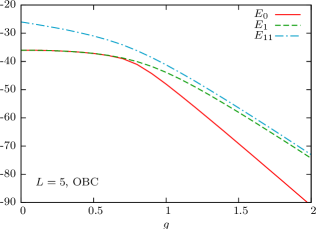
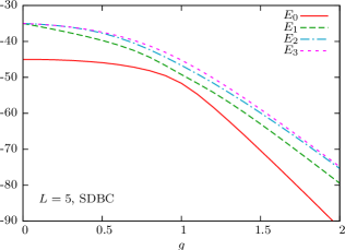
Figure 10: Energy levels of the $q$-state Potts chains with $L=5$, for OBC (Top) and SDBC (Bottom). (Top) The non degenerate, even, ground state level $E_{0}$ approaches the $(q-1)$ times degenerate multiplet of energy $E_{1}$ in the ordered phase $g<1$. (Bottom) The ground state, together with the levels $E_{1}$ and $E_{2}$, remain non degenerate at any $g>0$. $E_{3}$ is the lowest multiplet in the SDBC spectrum.

We use a standard implementation of the DMRG algorithm Sch-05 , adapted to the $q$-state Potts model. The computation involves solving eigenproblems of a size that rapidly grows with $q$ as $m^{2}q^{2}$, where $m$ is the number of states used in the DMRG base. We used up to $m=200$ for our DMRG computation of the $q=10$ Potts chains. In the worst case, corresponding to the longest chains, the truncation error (i.e., the sum of the discarded eigenvalues of the reduced density matrix) is $O(10^{-}9)$.

The energies $E_{n}$ of the excited states (and the differences $\Delta_{n}(L,g)=E_{n}-E_{0}$ as a consequence) are the quantities affected by larger convergence errors, whereas ground state properties, such as the ground state energy, the energy densities and the magnetizations, converge much more rapidly. The systematic error on a DMRG measurement can be estimated by looking at the progression of its convergence with successive iterations of the algorithm and as $m$ is gradually increased. We benchmarked this heuristics by comparing DMRG measurements with exact values on small chains, obtained with a diagonalization code.

To give an idea of the computational effort and accuracy of our numerical work, we mention that the DMRG computation for $L=35$ chain with SDBC at $g_{c}=1$ required a few hundred hours of CPU time of a standard processor to reach the truncation error of $2\times 10^{-9}$ for $m=200$. This allowed us to obtain the estimates $E_{0}=-346.484988(2)$ (where the number in parenthesis quantifies the systematic error due to the truncation of the states, corresponding to a relative precision of $0.6\times 10^{-8}$ for $E_{0}$), $E_{1}=-346.1459(7)$, $E_{2}=-345.696(2)$ for the lowest energy levels, thus $\Delta_{L}=0.3390(7)$ and $\Delta_{L,2}=0.789(2)$, and $m_{c}=0.529723(3)$, $e_{c}=0.593785(1)$ for the magnetization and energy density at the center of the chain. Note that this accuracy allows us to determine the energy differences of the lowest states with a relative precision of $O(10^{-3})$ for $\Delta_{L}=E_{1}-E_{0}$ and $O(10^{-2})$ for $\Delta_{L,2}=E_{2}-E_{0}$, which we deem sufficient for the observation of the scaling properties of the Potts model. We stress that the calculation of the energy differences, i.e. the gap, is essential to check the FSS ansatzes, thus we could not restrict our computations to the ground-state expectation values, which are usually much more precise.

Since the precision turns out to rapidly degrade with increasing $L$, making the computations very demanding to reach a satisfactory accuracy, we restricted our $q=10$ study to chain up $L=35$ sites. Fortunately, these relatively small sizes turn out to be already sufficient to provide a clear evidence of FSS at the FOQTs.

The low energy spectrum of the Potts chain with OBC is characterised by highly degenerate multiplets IS-83 (see also Fig. 10), which make DMRG computations particularly difficult. This is shown in Fig. 10, where we show the energy of the lowest levels for OBC and SDBC with $L=5$. Analogous behaviors apply for any finite $L$. The DMRG algorithm makes extensive use of sparse eigensolvers, whose rate of convergence and numerical stability depend on the spacing between the different eigenvalues. The system with SDBC is not affected by this issue thanks to the fixed spin at one end of the chain, which lifts the degeneracy. To give an idea of this effect, we performed a test run on a Potts chain with $q=10,L=9$ and $g=0.98$ with both SDBC and OBC, completing two sweeps with $m=20$ basis states and keeping all other simulation parameters unchanged. For $L\to\infty$ and $g<1$, the OBC system is expected to exhibit a $q$-times degenerate ground state. However, finite size corrections make the ground state non degenerate, with a $(q-1)$-times degenerate first excited level, as shown in Fig. 10. The run with SDBC takes approximately 180 seconds to complete, while the OBC run takes almost four times as long on the same machine. This efficiency gap is expected to widen for larger values of $m$, as the computation progresses. This problem can be partly mitigated by changing the internal parameters of the eigensolver routine, at the expense of some extra memory usage. For these reasons we obtain less precise results for the OBC. For example, for $L=35$ at $g=1$ we obtain $E_{0}=-342.1121(6)$ and $E_{1}=-340.645(1)$.

References

- (1) S. Sachdev, Quantum Phase Transitions, (Cambridge University Press. 2011, 2nd ed.)
- (2) M. Vojta, Rep. Prog. Phys. 66, 2069 (2003).
- (3) V. Piazza, V. Pellegrini, F. Beltram, W. Wegscheider, T. Jungwirth, and A.H. MacDonald, Nature 402, 638 (1999).
- (4) T. Vojta, D. Belitz, T.R. Kirkpatrick, and R. Narayanan, Ann. Phys. (Leipzig) 8, 593 (1999).
- (5) M. Uhlarz, C. Pfleiderer, and S.M. Hayden, Phys. Rev. Lett. 93, 256404 (2004).
- (6) C. Pfleiderer, J. Phys.: Cond. Matter 17, S987 (2005).
- (7) W. Knafo, S. Raymond, P. Lejay, and J. Flouquet, Nature Phys. 5, 753 (2009).
- (8) M. Campostrini, J. Nespolo, A. Pelissetto, and E. Vicari, Phys. Rev. Lett. 113, 070402 (2014).
- (9) S.L. Sondhi, S.M. Girvin, J.P. Carini, and D. Shahar, Rev. Mod. Phys. 69, 315 (1997).
- (10) M. Campostrini, A. Pelissetto and E. Vicari, Phys. Rev. B 89, 094516 (2014).
- (11) J. Sólyom and P. Pfeuty, Phys. Rev. B 24, 218 (1981).
- (12) F. Iglói and J. Sólyom, J. Phys. C: Solid State Phys. 16, 2833 (1983).
- (13) R.J. Baxter, J. Phys. C: Solid State Phys. 6, L445 (1973); R.J. Baxter, H.N.V. Temperley, and S.E. Ashley, Proc. R. Soc. Lond. A 538, 535 (1978).
- (14) F.Y. Wu, Rev. Mod. Phys. 54, 235 (1982).
- (15) U. Schollwöck, Rev. Mod. Phys. 77, 259 (2005).
- (16) R.B. Potts, Math. Proc. Camb. Phil. Soc. 48, 106 (1952)
- (17) F. Iglói and E. Carlon, Phys. Rev. B 59, 3783 (1999).
- (18) M. E. Fisher and M. N. Barber, Phys. Rev. Lett. 28, 1516 (1972).
- (19) M. N. Barber, in Phase Transitions and Critical Phenomena, edited by C. Domb and J. L. Lebowitz (Academic Press, New York, 1983), Vol. 8.
- (20) Finite Sise Scaling, edited by J. Cardy, (Elsevier, 1988).
- (21) V. Privman ed., Finite Size Scaling and Numerical Simulation of Statistical Systems (World Scientific, Singapore, 1990).
- (22) V. Privman, P. C. Hohenberg, and A. Aharony, in Phase Transitions and Critical Phenomena, Vol. 14, edited by C. Domb and J. L. Lebowitz (Academic Press, New York, 1991).
- (23) A. Pelissetto and E. Vicari, Phys. Rep. 368, 549 (2002).
- (24) B. Nienhuis and M. Nauenberg, Phys. Rev. Lett. 35, 477 (1975).
- (25) M.E. Fisher and A.N. Berker, Phys. Rev. B 26, 2507 (1982);
- (26) V. Privman and M. E. Fisher, J. Stat. Phys. 33, 385 (1983).
- (27) M. E. Fisher and V. Privman, Phys. Rev. B 32, 447 (1985).
- (28) M.S.S. Challa, D.P. Landau, and K. Binder, Phys. Rev. B 34, 1841 (1986).
- (29) J. Lee and J.M. Kosterlitz, Phys. Rev. B 43, 3265 (1991).
- (30) C. Borgs and R. Kotecký, Phys. Rev. Lett. 68, 1734 (1992).
- (31) A. Billoire, T. Neuhaus, and B.A. Berg, Nucl. Phys. B 396, 779 (1993).
- (32) K. Vollmayr, J.D. Reger, M. Scheucher, and K. Binder, Z. Phys. B 91, 113 (1993).
- (33) P. Calabrese, P. Parruccini, A. Pelissetto, and E. Vicari, Phys. Rev. B 70, 174439 (2004).
- (34) C. Bonati, M. D’Elia, and E. Vicari, Phys. Rev. E 89, 062132 (2014).
- (35) G.G. Cabrera and R. Jullien, Phys. Rev. B 35, 7062 (1987).
- (36) C.R. Laumann, R. Moessner, A. Scardicchio, and S. L. Sondhi, Phys. Rev. Lett. 109, 030502 (2012)
- (37) C. Zener, Proc. R. Soc. London, Ser A 137, 696 (1932); L. Landau, Phys. Z. Sowjetunion 2, 46 (1932).
- (38) F. Iachello and N. V. Zamfir, Phys. Rev. Lett. 92, 212501 (2004).
- (39) G.-D. Lin, C. Monroe, and L.-M. Duan, Phys. Rev. Lett. 106, 230402 (2011).
- (40) I.M. Georgescu, S. Ashhab, and F. Nori, Rev. Mod. Phys. 86, 153 (2014).
- (41) R. Islam, E.E. Edwards, K. Kim, S. Korenblit, C. Noh, H. Carmichael, G.-D. Lin, L.-M. Duan, C.-C. Joseph Wang, J.K. Freericks, and C. Monroe, Nature Comm. 2 377 (2011).
- (42) J. Simon, W.S. Bakr, R. Ma, M.E. Tai, P.M. Preiss, and M. Greiner, Nature 472, 307 (2011).
- (43) I. Bloch, Nature 453, 1016 (2008).
- (44) A.P. Young, S. Knysh, and V.N. Smelyanskiy, Phys. Rev. Lett. 104, 020502 (2010).
- (45) M.H.S. Amin and V. Choi, Phys. Rev. A 80, 062326 (2009).
- (46) M. Campostrini, J. Nespolo, A. Pelissetto, and E. Vicari, in preparation.