Light on the Infinite Group Relaxation

Abstract.

This is a survey on the infinite group problem, an infinite-dimensional relaxation of integer linear optimization problems introduced by Ralph Gomory and Ellis Johnson in their groundbreaking papers titled Some continuous functions related to corner polyhedra I, II [Math. Programming 3 (1972), 23–85, 359–389]. The survey presents the infinite group problem in the modern context of cut generating functions. It focuses on the recent developments, such as algorithms for testing extremality and breakthroughs for the $k$-row problem for general $k\geq 1$ that extend previous work on the single-row and two-row problems. The survey also includes some previously unpublished results; among other things, it unveils piecewise linear extreme functions with more than four different slopes. An interactive companion program, implemented in the open-source computer algebra package Sage, provides an updated compendium of known extreme functions.

1. Introduction

A recent line of activity in integer programming research is the development of cutting plane theory for general purpose mixed-integer linear programs. Although this theory was initiated by Gomory’s seminal work [31, 32, 33, 34, 35, 36] in integer programming, in the 1980s this general theory was overshadowed by the success of cutting planes for specially structured combinatorial optimization problems such as the TSP, the stable set problem and the knapsack problem. A re-evaluation of Gomory’s cutting planes in the 1990s [7] led to a renewed interest in general purpose cutting plane theory. A key turning point in the 2000s was the emphasis on the so-called multi-row cuts, which hold the promise of making significant breakthroughs in algorithms for solving large-scale mixed-integer programs. The last decade has witnessed considerable progress for multi-row cuts. This recent research is collectively referred to under the label of cut-generating functions, a term coined by Cornuéjols [21].

A central problem and a driving force behind this line of work has been the so-called infinite group problem (or infinite relaxation), introduced by Gomory and Johnson in two seminal papers in 1972 [37, 38]. In this sense, the infinite group problem was a visionary contribution that anticipated this modern trend in integer programming decades earlier. To make further progress in the elaborate research program of cut-generating functions, it is imperative to understand the infinite group problem even better. The bulk of Gomory and Johnson’s contributions were in the single-row infinite group problem, and until recently the theory behind the multi-row infinite group problem was mostly in the dark. With the modern focus on multi-row cuts within cut-generating functions, it is very important to understand the multi-row infinite group problem. The last decade has seen some excellent progress in this question, and this survey attempts to present this story.

1.1. Cut-generating function pairs

We begin with a quick overview of the cut-generating function approach to unifying cutting plane theory. Let $d\in\mathbb{N}$ and $I$ be a fixed subset of $\{1,\ldots,d\}$. A mixed-integer optimization problem of the form

$$\max\{\,\mathchoice{\mbox{\boldmath$\displaystyle\bf c$}}{\mbox{\boldmath$\textstyle\bf c$}}{\mbox{\boldmath$\scriptstyle\bf c$}}{\mbox{\boldmath$\scriptscriptstyle\bf c$}}\cdot\mathchoice{\mbox{\boldmath$\displaystyle\bf x$}}{\mbox{\boldmath$\textstyle\bf x$}}{\mbox{\boldmath$\scriptstyle\bf x$}}{\mbox{\boldmath$\scriptscriptstyle\bf x$}}\mid A\mathchoice{\mbox{\boldmath$\displaystyle\bf x$}}{\mbox{\boldmath$\textstyle\bf x$}}{\mbox{\boldmath$\scriptstyle\bf x$}}{\mbox{\boldmath$\scriptscriptstyle\bf x$}}=\mathchoice{\mbox{\boldmath$\displaystyle\bf b$}}{\mbox{\boldmath$\textstyle\bf b$}}{\mbox{\boldmath$\scriptstyle\bf b$}}{\mbox{\boldmath$\scriptscriptstyle\bf b$}},\ \mathchoice{\mbox{\boldmath$\displaystyle\bf x$}}{\mbox{\boldmath$\textstyle\bf x$}}{\mbox{\boldmath$\scriptstyle\bf x$}}{\mbox{\boldmath$\scriptscriptstyle\bf x$}}\in\mathbb{R}^{d}_{+},\ x_{i}\in\mathbb{Z}\quad\forall i\in I\,\}$$ (1)

is first solved by ignoring the integrality constraints and using the simplex algorithm. This leads to a simplex tableau reformulation:

$$A_{B}^{-1}A_{N}\mathchoice{\mbox{\boldmath$\displaystyle\bf x$}}{\mbox{\boldmath$\textstyle\bf x$}}{\mbox{\boldmath$\scriptstyle\bf x$}}{\mbox{\boldmath$\scriptscriptstyle\bf x$}}_{N}=A_{B}^{-1}\mathchoice{\mbox{\boldmath$\displaystyle\bf b$}}{\mbox{\boldmath$\textstyle\bf b$}}{\mbox{\boldmath$\scriptstyle\bf b$}}{\mbox{\boldmath$\scriptscriptstyle\bf b$}}\,-\,\mathchoice{\mbox{\boldmath$\displaystyle\bf x$}}{\mbox{\boldmath$\textstyle\bf x$}}{\mbox{\boldmath$\scriptstyle\bf x$}}{\mbox{\boldmath$\scriptscriptstyle\bf x$}}_{B},\quad\mathchoice{\mbox{\boldmath$\displaystyle\bf x$}}{\mbox{\boldmath$\textstyle\bf x$}}{\mbox{\boldmath$\scriptstyle\bf x$}}{\mbox{\boldmath$\scriptscriptstyle\bf x$}}_{B\cap I}\in\mathbb{Z}_{+}^{B\cap I},\ \mathchoice{\mbox{\boldmath$\displaystyle\bf x$}}{\mbox{\boldmath$\textstyle\bf x$}}{\mbox{\boldmath$\scriptstyle\bf x$}}{\mbox{\boldmath$\scriptscriptstyle\bf x$}}_{B\setminus I}\in\mathbb{R}_{+}^{B\setminus I},\ \mathchoice{\mbox{\boldmath$\displaystyle\bf x$}}{\mbox{\boldmath$\textstyle\bf x$}}{\mbox{\boldmath$\scriptstyle\bf x$}}{\mbox{\boldmath$\scriptscriptstyle\bf x$}}_{N\cap I}\in\mathbb{Z}_{+}^{N\cap I},\ \mathchoice{\mbox{\boldmath$\displaystyle\bf x$}}{\mbox{\boldmath$\textstyle\bf x$}}{\mbox{\boldmath$\scriptstyle\bf x$}}{\mbox{\boldmath$\scriptscriptstyle\bf x$}}_{N\setminus I}\in\mathbb{R}_{+}^{N\setminus I}$$ (2)

where the subscripts $B$ and $N$ denote the basic and non-basic parts of the solution $\textstyle\bf x$ and matrix $A$, respectively. The following change of notation will be convenient: let $k=|B|$, $m=|N\setminus I|$, $\ell=|N\cap I|$, let $R$ denote the submatrix of $A^{-1}_{B}A_{N}$ indexed by $N\setminus I$, $P$ denote the submatrix of $A^{-1}_{B}A_{N}$ indexed by $N\cap I$, and set $\bar{S}=A^{-1}_{B}\mathchoice{\mbox{\boldmath$\displaystyle\bf b$}}{\mbox{\boldmath$\textstyle\bf b$}}{\mbox{\boldmath$\scriptstyle\bf b$}}{\mbox{\boldmath$\scriptscriptstyle\bf b$}}-(\mathbb{Z}_{+}^{B\cap I}\times\mathbb{R}_{+}^{B\setminus I})$. Then in the new notation, we describe system (2) as

$$X_{\bar{S}}(R,P):=\left\{\,(\mathchoice{\mbox{\boldmath$\displaystyle\bf s$}}{\mbox{\boldmath$\textstyle\bf s$}}{\mbox{\boldmath$\scriptstyle\bf s$}}{\mbox{\boldmath$\scriptscriptstyle\bf s$}},\mathchoice{\mbox{\boldmath$\displaystyle\bf y$}}{\mbox{\boldmath$\textstyle\bf y$}}{\mbox{\boldmath$\scriptstyle\bf y$}}{\mbox{\boldmath$\scriptscriptstyle\bf y$}})\in\mathbb{R}_{+}^{m}\times\mathbb{Z}_{+}^{\ell}\,\mid\,R\mathchoice{\mbox{\boldmath$\displaystyle\bf s$}}{\mbox{\boldmath$\textstyle\bf s$}}{\mbox{\boldmath$\scriptstyle\bf s$}}{\mbox{\boldmath$\scriptscriptstyle\bf s$}}+P\mathchoice{\mbox{\boldmath$\displaystyle\bf y$}}{\mbox{\boldmath$\textstyle\bf y$}}{\mbox{\boldmath$\scriptstyle\bf y$}}{\mbox{\boldmath$\scriptscriptstyle\bf y$}}\in\bar{S}\,\right\}.$$ (3)

In the following, we will consider general systems of the form (3), where $m,\ell\in\mathbb{Z}_{+}$ and $k\in\mathbb{N}$, $R\in\mathbb{R}^{k\times m}$ and $P\in\mathbb{R}^{k\times\ell}$ are matrices, and $\bar{S}$ is a closed subset of $\mathbb{R}^{k}$ such that ${\mathchoice{\mbox{\boldmath$\displaystyle\bf 0$}}{\mbox{\boldmath$\textstyle\bf 0$}}{\mbox{\boldmath$\scriptstyle\bf 0$}}{\mbox{\boldmath$\scriptscriptstyle\bf 0$}}}\not\in\bar{S}$. Instead of using the full simplex tableau (2), one can as well consider relaxations of (2), for example by taking a subset of the rows only. In the simplest case, one focuses on only one row, i.e., $k=1$.

We denote the columns of matrices $R$ and $P$ by $\mathchoice{\mbox{\boldmath$\displaystyle\bf r$}}{\mbox{\boldmath$\textstyle\bf r$}}{\mbox{\boldmath$\scriptstyle\bf r$}}{\mbox{\boldmath$\scriptscriptstyle\bf r$}}^{1},\ldots,\mathchoice{\mbox{\boldmath$\displaystyle\bf r$}}{\mbox{\boldmath$\textstyle\bf r$}}{\mbox{\boldmath$\scriptstyle\bf r$}}{\mbox{\boldmath$\scriptscriptstyle\bf r$}}^{m}$ and $\mathchoice{\mbox{\boldmath$\displaystyle\bf p$}}{\mbox{\boldmath$\textstyle\bf p$}}{\mbox{\boldmath$\scriptstyle\bf p$}}{\mbox{\boldmath$\scriptscriptstyle\bf p$}}^{1},\ldots,\mathchoice{\mbox{\boldmath$\displaystyle\bf p$}}{\mbox{\boldmath$\textstyle\bf p$}}{\mbox{\boldmath$\scriptstyle\bf p$}}{\mbox{\boldmath$\scriptscriptstyle\bf p$}}^{\ell},$ respectively. Given $k\in\mathbb{N}$ and $\bar{S}\subseteq\mathbb{R}^{k}$, a cut-generating function pair (or simply, cut-generating pair) $(\psi,\pi)$ for $\bar{S}$ is a pair of functions $\psi,\pi\colon\mathbb{R}^{n}\to\mathbb{R}$ such that

$$\sum_{i=1}^{m}\psi(\mathchoice{\mbox{\boldmath$\displaystyle\bf r$}}{\mbox{\boldmath$\textstyle\bf r$}}{\mbox{\boldmath$\scriptstyle\bf r$}}{\mbox{\boldmath$\scriptscriptstyle\bf r$}}^{i})s_{i}+\sum_{j=1}^{\ell}\pi(\mathchoice{\mbox{\boldmath$\displaystyle\bf p$}}{\mbox{\boldmath$\textstyle\bf p$}}{\mbox{\boldmath$\scriptstyle\bf p$}}{\mbox{\boldmath$\scriptscriptstyle\bf p$}}^{j})y_{j}\geq 1$$ (4)

is a valid inequality (also called a cutting plane or cut) for the set $X_{\bar{S}}(R,P)$ for every choice of $m,\ell\in\mathbb{Z}_{+}$ and for all matrices $R\in\mathbb{R}^{k\times m}$ and $P\in\mathbb{R}^{k\times\ell}$. We emphasize that cut-generating pairs depend on $k$ and $\bar{S}$ and do not depend on $m,\ell$, $R$ and $P$. A priori it is not clear that such cut-generating function pairs can exist. However, it has been observed that for many special cases of model (3) the convex hull of points in $X_{\bar{S}}(R,P)$ can be completely described using cut-generating functions, i.e., not only do they exist, but they are sufficient for the purposes of optimization from a theoretical perspective.

Gomory and Johnson’s joint work in the 1970s [37, 38], together with Johnson’s independent results [43] in the same decade, shows that cut-generating pairs can be understood by studying infinite-dimensional convex sets parameterized by $k\in\mathbb{N}$ and $\bar{S}\subseteq\mathbb{R}^{k}$. For any index set $I$ (not necessarily finite), $\mathbb{R}^{I}$ will denote the vector space of all real-valued functions with domain $I$, and $\mathbb{R}^{(I)}$ will denote the subspace of real-valued functions with domain $I$ that have finite support, i.e., functions that take value zero except on a finite set. For example, $\mathbb{R}^{(\mathbb{R}^{k})}$ is the set of all functions $s\colon\mathbb{R}^{k}\to\mathbb{R}$ with finite support. The object of interest is

$$X_{\bar{S}}:=\biggl{\{}\,(s,y)\in\mathbb{R}^{(\mathbb{R}^{k})}\times\mathbb{R}^{(\mathbb{R}^{k})}\mathrel{\bigg{|}}\sum_{\mathchoice{\mbox{\boldmath$\displaystyle\bf r$}}{\mbox{\boldmath$\textstyle\bf r$}}{\mbox{\boldmath$\scriptstyle\bf r$}}{\mbox{\boldmath$\scriptscriptstyle\bf r$}}\in\mathbb{R}^{k}}\mathchoice{\mbox{\boldmath$\displaystyle\bf r$}}{\mbox{\boldmath$\textstyle\bf r$}}{\mbox{\boldmath$\scriptstyle\bf r$}}{\mbox{\boldmath$\scriptscriptstyle\bf r$}}s(\mathchoice{\mbox{\boldmath$\displaystyle\bf r$}}{\mbox{\boldmath$\textstyle\bf r$}}{\mbox{\boldmath$\scriptstyle\bf r$}}{\mbox{\boldmath$\scriptscriptstyle\bf r$}})+\sum_{\mathchoice{\mbox{\boldmath$\displaystyle\bf p$}}{\mbox{\boldmath$\textstyle\bf p$}}{\mbox{\boldmath$\scriptstyle\bf p$}}{\mbox{\boldmath$\scriptscriptstyle\bf p$}}\in\mathbb{R}^{k}}\mathchoice{\mbox{\boldmath$\displaystyle\bf p$}}{\mbox{\boldmath$\textstyle\bf p$}}{\mbox{\boldmath$\scriptstyle\bf p$}}{\mbox{\boldmath$\scriptscriptstyle\bf p$}}y(\mathchoice{\mbox{\boldmath$\displaystyle\bf p$}}{\mbox{\boldmath$\textstyle\bf p$}}{\mbox{\boldmath$\scriptstyle\bf p$}}{\mbox{\boldmath$\scriptscriptstyle\bf p$}})\in\bar{S},\,\,s(\mathchoice{\mbox{\boldmath$\displaystyle\bf r$}}{\mbox{\boldmath$\textstyle\bf r$}}{\mbox{\boldmath$\scriptstyle\bf r$}}{\mbox{\boldmath$\scriptscriptstyle\bf r$}})\in\mathbb{R}_{+}\;\forall\mathchoice{\mbox{\boldmath$\displaystyle\bf r$}}{\mbox{\boldmath$\textstyle\bf r$}}{\mbox{\boldmath$\scriptstyle\bf r$}}{\mbox{\boldmath$\scriptscriptstyle\bf r$}}\in\mathbb{R}^{k},\ y(\mathchoice{\mbox{\boldmath$\displaystyle\bf p$}}{\mbox{\boldmath$\textstyle\bf p$}}{\mbox{\boldmath$\scriptstyle\bf p$}}{\mbox{\boldmath$\scriptscriptstyle\bf p$}})\in\mathbb{Z}_{+}\;\forall\mathchoice{\mbox{\boldmath$\displaystyle\bf p$}}{\mbox{\boldmath$\textstyle\bf p$}}{\mbox{\boldmath$\scriptstyle\bf p$}}{\mbox{\boldmath$\scriptscriptstyle\bf p$}}\in\mathbb{R}^{k}\,\biggr{\}}.$$ (5)

The convex hull of points in $X_{\bar{S}}$ is an infinite-dimensional convex set in $\mathbb{R}^{(\mathbb{R}^{k})}\times\mathbb{R}^{(\mathbb{R}^{k})}$ that contains the convex hull of every $X_{\bar{S}}(R,P)$ (for every choice of $R$ and $P$) as a finite-dimensional face. Cut generating function pairs can then be interpreted as halfspaces in the vector space $\mathbb{R}^{(\mathbb{R}^{k})}\times\mathbb{R}^{(\mathbb{R}^{k})}$ that contain $X_{\bar{S}}$.

1.2. Approaches to understanding cut-generating function pairs

The setting of $\operatorname{conv}(X_{\bar{S}})$ where $\bar{S}$ is a translate of $\mathbb{Z}^{k}$ has received the most attention in the literature. Fix a point ${\mathchoice{\mbox{\boldmath$\displaystyle\bf f$}}{\mbox{\boldmath$\textstyle\bf f$}}{\mbox{\boldmath$\scriptstyle\bf f$}}{\mbox{\boldmath$\scriptscriptstyle\bf f$}}}\in\mathbb{R}^{k}\setminus\mathbb{Z}^{k}$ and let $\bar{S}={\mathchoice{\mbox{\boldmath$\displaystyle\bf f$}}{\mbox{\boldmath$\textstyle\bf f$}}{\mbox{\boldmath$\scriptstyle\bf f$}}{\mbox{\boldmath$\scriptscriptstyle\bf f$}}}+\mathbb{Z}^{k}$. Two distinct approaches have emerged within the study of the facial structure of $\operatorname{conv}(X_{\bar{S}})$, which we will compare below.

1. The infinite group problem. Gomory and Johnson, in their work in [37, 38], study the infinite group problem, which appears as the face of $\operatorname{conv}(X_{\bar{S}})$ given by $\operatorname{conv}(X_{\bar{S}})\cap\big{\{}\,(s,y)\in\mathbb{R}^{(\mathbb{R}^{k})}\times\mathbb{R}^{(\mathbb{R}^{k})}\mid s=0\,\big{\}}$. This produces cut-generating functions $\pi\colon\mathbb{R}^{k}\to\mathbb{R}$ that are useful for the study of pure integer optimization problems. The structure of these functions $\pi$ can be very complicated; it is the main topic of our survey.

   By Johnson’s fundamental work [43], we know that these functions $\pi$ can then be easily lifted to strong cut-generating pairs $(\psi,\pi)$ for mixed-integer optimization problems using closed form formulas.

2. Intersection cuts. Another approach to cut-generating pairs has its roots in Balas’ work on intersection cuts [6] and Balas and Jeroslow’s work on monoidal strengthening [8]. More recent work by Andersen, Louveaux, Weismantel, and Wolsey [3] renewed the interest in this approach. Borozan and Cornuéjols [19] put it in the framework of cut generating functions, and Dey and Wolsey [30] interpreted monoidal strengthening in this setting. This line of research was developed further in many papers, including [10, 11, 9, 13, 23, 29].

   Consider again the case $\bar{S}={\mathchoice{\mbox{\boldmath$\displaystyle\bf f$}}{\mbox{\boldmath$\textstyle\bf f$}}{\mbox{\boldmath$\scriptstyle\bf f$}}{\mbox{\boldmath$\scriptscriptstyle\bf f$}}}+\mathbb{Z}^{k}$. Then the face of $\operatorname{conv}(X_{\bar{S}})$ given by $\operatorname{conv}(X_{\bar{S}})\cap\big{\{}\,(s,y)\in\mathbb{R}^{(\mathbb{R}^{k})}\times\mathbb{R}^{(\mathbb{R}^{k})}\mid y=0\,\big{\}}$ is studied first, giving cut-generating functions $\psi\colon\mathbb{R}^{k}\to\mathbb{R}$. They are obtained as the gauge functions of maximal lattice-free convex bodies. The functions $\psi$ are then lifted to cut-generating pairs $(\psi,\pi)$ for $X_{\bar{S}}$.

   The advantage of the intersection cut approach, compared with Gomory–Johnson’s infinite group problem, is that the gauge functions $\psi$ can be evaluated using simpler formulas. Further, generalizations have been studied in which the set $\bar{S}$ is allowed to be more general than just a translated lattice – the most frequently studied $\bar{S}$ is of the form $C\cap({\mathchoice{\mbox{\boldmath$\displaystyle\bf f$}}{\mbox{\boldmath$\textstyle\bf f$}}{\mbox{\boldmath$\scriptstyle\bf f$}}{\mbox{\boldmath$\scriptscriptstyle\bf f$}}}+\mathbb{Z}^{k})$ where $C$ is a convex subset of $\mathbb{R}^{k}$ and ${\mathchoice{\mbox{\boldmath$\displaystyle\bf f$}}{\mbox{\boldmath$\textstyle\bf f$}}{\mbox{\boldmath$\scriptstyle\bf f$}}{\mbox{\boldmath$\scriptscriptstyle\bf f$}}}\in\mathbb{R}^{k}\setminus\mathbb{Z}^{k}$ (for example, $C=\mathbb{R}^{k}_{+}$ would correspond to model (2)). In this case, the cut-generating functions are obtained from so-called maximal $\bar{S}$-free convex sets.

   The drawback of the intersection cut approach is that lifting a gauge function $\psi$ to a strong cut-generating pair $(\psi,\pi)$ can be rather difficult. This difficulty has been recently studied by [9, 13, 23, 5]. Moreover, this approach produces a much smaller subset of cut-generating pairs as compared with the infinite group approach when $\bar{S}$ is a translated lattice. In this case, there exist undominated cut-generating pairs $(\psi,\pi)$ where $\psi$ is not the gauge of a maximal lattice-free set – these can still be obtained in the context of the infinite group problem. In contrast the approach outlined above starts with a function $\psi$ that is the gauge function of a maximal lattice-free set, and so the approach cannot derive such cut-generating functions.

Remark 1.0.

The study of cut-generating functions for $k=1$ is referred to as the single-row problem, and the general $k\geq 2$ case is referred to as the multi-row problem in the literature. Algorithms used in practice for solving mixed-integer problems have so far used only insights from the single-row problem. It is believed that the general multi-row analysis can lead to stronger cutting planes that can significantly boost the performance of state-of-the-art algorithms.

1.3. Outline of the survey

We will survey the recent progress made on the infinite group problem approach described in subsection 1.2. We view this as a follow-up to two excellent surveys, the first by Conforti, Cornuéjols, and Zambelli [22], which discusses the basic structure of the corner polyhedron and its relation with cut-generating functions, and the second by Richard and Dey [48], which focuses on the group-theoretic approach. Our survey focuses on the milestones that have been reached since [22, 48] were written. Although we do not intend [22, 48] to be prerequisites to this article, the reader who is familiar with the material from [22, 48] will certainly have a better context for the current article. The reader may use Table 6 in Appendix B as a reference to notation in these surveys and other literature.

Section 2 formally introduces the problem, the main objects of study such as valid functions, minimal valid functions, extreme functions, and facets, and their basic properties. We conclude the section with a discussion of families of valid functions and some open questions (subsection 2.4). The discussion references a compendium that summarizes known families from the literature (Appendix A), and contains some previously unknown families such as extreme functions with 5 slopes and some discontinuous extreme functions with left and right discontinuity at the origin. Section 3 introduces the notation and concepts from discrete geometry required for analyzing the problem, and collects foundational techniques for the general $k$-row problem. Section 4 surveys higher-dimensional variants of the celebrated Interval Lemma. Section 5 introduces one of the most general sufficient conditions for the fundamental notion of extremality, illustrating how all the techniques introduced in the previous sections come together to analyze extremality. Section 6 investigates some analytic properties of the problem and demonstrates the use of analytical ideas to construct extreme functions. Sections 7 and 8 discuss important algorithmic and structural results known for the one-row and two-row problems. These results are based on recent breakthroughs in [15, 14, 16].

We highlight results that are new in this survey with the annotation “New result $\clubsuit$”. To the best of our knowledge, these do not appear elsewhere in the literature.

Due to constraints of space, we must limit the topics covered in this survey. We briefly mention some of the important highlights in the literature that are not discussed in this survey. A wealth of results on the finite group problem are closely related to the infinite group problem. We invite the reader to explore the survey by Richard and Dey [48] for more details about this direction. Furthermore, we focus on the structural results of the infinite group problem, as opposed to the implementation of these results in algorithms to solve integer programming problems. This includes the so-called shooting experiments discussed in [40] to empirically judge quality of the cutting planes, and the discussion of relative strength in [39, section 6].

2. The Infinite Group Problem

As stated in subsection 1.2, Gomory and Johnson introduced the so-called infinite group problem. It has its roots in Gomory’s group problem [35], which was introduced by him as an algebraic relaxation of pure integer linear optimization problems. We introduce this next as it will be useful for formulating many of our results in a unified language. One considers an abelian group $G$, written additively, and studies the set of functions $y\colon G\to\mathbb{R}$ satisfying the following constraints:

$$\sum_{{\mathchoice{\mbox{\boldmath$\displaystyle\bf r$}}{\mbox{\boldmath$\textstyle\bf r$}}{\mbox{\boldmath$\scriptstyle\bf r$}}{\mbox{\boldmath$\scriptscriptstyle\bf r$}}}\in G}{\mathchoice{\mbox{\boldmath$\displaystyle\bf r$}}{\mbox{\boldmath$\textstyle\bf r$}}{\mbox{\boldmath$\scriptstyle\bf r$}}{\mbox{\boldmath$\scriptscriptstyle\bf r$}}}\,y({\mathchoice{\mbox{\boldmath$\displaystyle\bf r$}}{\mbox{\boldmath$\textstyle\bf r$}}{\mbox{\boldmath$\scriptstyle\bf r$}}{\mbox{\boldmath$\scriptscriptstyle\bf r$}}})\in\mathchoice{\mbox{\boldmath$\displaystyle\bf f$}}{\mbox{\boldmath$\textstyle\bf f$}}{\mbox{\boldmath$\scriptstyle\bf f$}}{\mbox{\boldmath$\scriptscriptstyle\bf f$}}+S$$ (6)

$$y({\mathchoice{\mbox{\boldmath$\displaystyle\bf r$}}{\mbox{\boldmath$\textstyle\bf r$}}{\mbox{\boldmath$\scriptstyle\bf r$}}{\mbox{\boldmath$\scriptscriptstyle\bf r$}}})\in\mathbb{Z}_{+}\ \ \textrm{for all ${\mathchoice{\mbox{\boldmath$\displaystyle\bf r$}}{\mbox{\boldmath$\textstyle\bf r$}}{\mbox{\boldmath$\scriptstyle\bf r$}}{\mbox{\boldmath$\scriptscriptstyle\bf r$}}}\in G$}$$

$$y\textrm{ has finite support},$$

where $S$ is a subgroup of $G$ and $\textstyle\bf f$ is a given element in $G\setminus S$; so $\mathchoice{\mbox{\boldmath$\displaystyle\bf f$}}{\mbox{\boldmath$\textstyle\bf f$}}{\mbox{\boldmath$\scriptstyle\bf f$}}{\mbox{\boldmath$\scriptscriptstyle\bf f$}}+S$ is the coset containing the element $\textstyle\bf f$. We are interested in studying the convex hull $R_{\mathchoice{\mbox{\boldmath$\displaystyle\bf f$}}{\mbox{\boldmath$\textstyle\bf f$}}{\mbox{\boldmath$\scriptstyle\bf f$}}{\mbox{\boldmath$\scriptscriptstyle\bf f$}}}(G,S)$ of the set of all functions $y\colon G\to\mathbb{R}$ satisfying the constraints in (6). $R_{\mathchoice{\mbox{\boldmath$\displaystyle\bf f$}}{\mbox{\boldmath$\textstyle\bf f$}}{\mbox{\boldmath$\scriptstyle\bf f$}}{\mbox{\boldmath$\scriptscriptstyle\bf f$}}}(G,S)$ is a convex subset of the vector space $\mathbb{R}^{(G)}$, which is infinite-dimensional when $G$ is an infinite group, i.e., of infinite order. The nomenclature $k$-row infinite group problem is reserved for the situation when $G=\mathbb{R}^{k}$ is taken to be the group of real $k$-dimensional vectors under addition, and $S=\mathbb{Z}^{k}$ is the subgroup of the integer vectors. When $k=1$, we refer to it as the single-row infinite group problem. Recall that the connection with the cut-generating function model (3) is made by setting $\bar{S}={\mathchoice{\mbox{\boldmath$\displaystyle\bf f$}}{\mbox{\boldmath$\textstyle\bf f$}}{\mbox{\boldmath$\scriptstyle\bf f$}}{\mbox{\boldmath$\scriptscriptstyle\bf f$}}}+S$, whence we get $R_{\mathchoice{\mbox{\boldmath$\displaystyle\bf f$}}{\mbox{\boldmath$\textstyle\bf f$}}{\mbox{\boldmath$\scriptstyle\bf f$}}{\mbox{\boldmath$\scriptscriptstyle\bf f$}}}(G,S)$ as the projection of $\operatorname{conv}(X_{\bar{S}})\cap\big{\{}(s,y)\in\mathbb{R}^{(\mathbb{R}^{k})}\times\mathbb{R}^{(\mathbb{R}^{k})}\mid s=0\big{\}}$ onto the $y$ space.

Remark 2.0.

Note that there is a correspondence between the sets $R_{\mathchoice{\mbox{\boldmath$\displaystyle\bf f$}}{\mbox{\boldmath$\textstyle\bf f$}}{\mbox{\boldmath$\scriptstyle\bf f$}}{\mbox{\boldmath$\scriptscriptstyle\bf f$}}}(G,S)$ and $R_{\bar{\mathchoice{\mbox{\boldmath$\displaystyle\bf f$}}{\mbox{\boldmath$\textstyle\bf f$}}{\mbox{\boldmath$\scriptstyle\bf f$}}{\mbox{\boldmath$\scriptscriptstyle\bf f$}}}}(G/S,0)$ where $G/S$ is the quotient group with respect to the (normal) subgroup $S$ and $\bar{\mathchoice{\mbox{\boldmath$\displaystyle\bf f$}}{\mbox{\boldmath$\textstyle\bf f$}}{\mbox{\boldmath$\scriptstyle\bf f$}}{\mbox{\boldmath$\scriptscriptstyle\bf f$}}}$ is the element corresponding to the coset ${\mathchoice{\mbox{\boldmath$\displaystyle\bf f$}}{\mbox{\boldmath$\textstyle\bf f$}}{\mbox{\boldmath$\scriptstyle\bf f$}}{\mbox{\boldmath$\scriptscriptstyle\bf f$}}}+S$, by standard aggregation of variables.

In the earlier literature on the infinite group problem, the aggregated formulation $R_{\bar{\mathchoice{\mbox{\boldmath$\displaystyle\bf f$}}{\mbox{\boldmath$\textstyle\bf f$}}{\mbox{\boldmath$\scriptstyle\bf f$}}{\mbox{\boldmath$\scriptscriptstyle\bf f$}}}}(\mathbb{R}^{k}/\mathbb{Z}^{k},0)$ was used. The quotient $\mathbb{R}^{k}/\mathbb{Z}^{k}$ is the $k$-dimensional torus; it can be identified with the half-open unit cube $[0,1)^{k}$, using coordinatewise arithmetic modulo 1. In this survey, however, we follow the trend in the recent literature [22, 15, 14, 16] to work with $R_{\mathchoice{\mbox{\boldmath$\displaystyle\bf f$}}{\mbox{\boldmath$\textstyle\bf f$}}{\mbox{\boldmath$\scriptstyle\bf f$}}{\mbox{\boldmath$\scriptscriptstyle\bf f$}}}(\mathbb{R}^{k},\mathbb{Z}^{k})$ instead. This removes the need for complicated notation for mapping between elements of $\mathbb{R}^{k}$ and elements of $\mathbb{R}^{k}/\mathbb{Z}^{k}$ (see Table 6 for an overview), and for complicated geometric notions, such as “wrap-around” line segments in Johnson’s cylindrical space [39], in favor of the standard mathematical language of periodic, locally finite polyhedral complexes on $\mathbb{R}^{k}$ (subsection 3.1). We pay a small price for the simplicity and precision of this approach: We will often work with infinite objects where finite objects would suffice. However, it is very easy to go back to finite objects in the moments when we want to state algorithms.

The aggregated formulation is still of interest for the case where $G/S$ is a finite group, as then $R_{\bar{\mathchoice{\mbox{\boldmath$\displaystyle\bf f$}}{\mbox{\boldmath$\textstyle\bf f$}}{\mbox{\boldmath$\scriptstyle\bf f$}}{\mbox{\boldmath$\scriptscriptstyle\bf f$}}}}(G/S,0)$ is finite-dimensional and thus amenable to polyhedral techniques. This case is referred to as a finite group problem; it will appear in subsection 8.1. Due to the correspondence between the sets $R_{\mathchoice{\mbox{\boldmath$\displaystyle\bf f$}}{\mbox{\boldmath$\textstyle\bf f$}}{\mbox{\boldmath$\scriptstyle\bf f$}}{\mbox{\boldmath$\scriptscriptstyle\bf f$}}}(G,S)$ and $R_{\bar{\mathchoice{\mbox{\boldmath$\displaystyle\bf f$}}{\mbox{\boldmath$\textstyle\bf f$}}{\mbox{\boldmath$\scriptstyle\bf f$}}{\mbox{\boldmath$\scriptscriptstyle\bf f$}}}}(G/S,0)$, we shall also refer to $R_{\mathchoice{\mbox{\boldmath$\displaystyle\bf f$}}{\mbox{\boldmath$\textstyle\bf f$}}{\mbox{\boldmath$\scriptstyle\bf f$}}{\mbox{\boldmath$\scriptscriptstyle\bf f$}}}(G,S)$ as a finite group problem whenever $S$ has finite index in $G$, i.e., $G/S$ is a finite group.

2.1. Valid inequalities and valid functions

Following Gomory and Johnson, we are interested in the description of $R_{\mathchoice{\mbox{\boldmath$\displaystyle\bf f$}}{\mbox{\boldmath$\textstyle\bf f$}}{\mbox{\boldmath$\scriptstyle\bf f$}}{\mbox{\boldmath$\scriptscriptstyle\bf f$}}}(G,S)$ as the intersection of halfspaces in $\mathbb{R}^{(G)}$. We first describe the general form that these halfspaces take and then a standard normalization that leads to the idea of cut-generating functions.

2.1.1. Valid inequalities

Any halfspace in $\mathbb{R}^{(G)}$ is given by a pair $(\pi,\alpha)$, where $\pi\in\mathbb{R}^{G}$ and $\alpha\in\mathbb{R}$, and the halfspace is the set of all $y\in\mathbb{R}^{(G)}$ that satisfy $\sum_{{\mathchoice{\mbox{\boldmath$\displaystyle\bf r$}}{\mbox{\boldmath$\textstyle\bf r$}}{\mbox{\boldmath$\scriptstyle\bf r$}}{\mbox{\boldmath$\scriptscriptstyle\bf r$}}}\in G}\pi({\mathchoice{\mbox{\boldmath$\displaystyle\bf r$}}{\mbox{\boldmath$\textstyle\bf r$}}{\mbox{\boldmath$\scriptstyle\bf r$}}{\mbox{\boldmath$\scriptscriptstyle\bf r$}}})y({\mathchoice{\mbox{\boldmath$\displaystyle\bf r$}}{\mbox{\boldmath$\textstyle\bf r$}}{\mbox{\boldmath$\scriptstyle\bf r$}}{\mbox{\boldmath$\scriptscriptstyle\bf r$}}})\geq\alpha$. The left-hand side of the inequality is a finite sum because $y$ has finite support. Such an inequality is called a valid inequality for $R_{\mathchoice{\mbox{\boldmath$\displaystyle\bf f$}}{\mbox{\boldmath$\textstyle\bf f$}}{\mbox{\boldmath$\scriptstyle\bf f$}}{\mbox{\boldmath$\scriptscriptstyle\bf f$}}}(G,S)$ if $\sum_{{\mathchoice{\mbox{\boldmath$\displaystyle\bf r$}}{\mbox{\boldmath$\textstyle\bf r$}}{\mbox{\boldmath$\scriptstyle\bf r$}}{\mbox{\boldmath$\scriptscriptstyle\bf r$}}}\in G}\pi({\mathchoice{\mbox{\boldmath$\displaystyle\bf r$}}{\mbox{\boldmath$\textstyle\bf r$}}{\mbox{\boldmath$\scriptstyle\bf r$}}{\mbox{\boldmath$\scriptscriptstyle\bf r$}}})y({\mathchoice{\mbox{\boldmath$\displaystyle\bf r$}}{\mbox{\boldmath$\textstyle\bf r$}}{\mbox{\boldmath$\scriptstyle\bf r$}}{\mbox{\boldmath$\scriptscriptstyle\bf r$}}})\geq\alpha$ for all $y\in R_{\mathchoice{\mbox{\boldmath$\displaystyle\bf f$}}{\mbox{\boldmath$\textstyle\bf f$}}{\mbox{\boldmath$\scriptstyle\bf f$}}{\mbox{\boldmath$\scriptscriptstyle\bf f$}}}(G,S)$, i.e., $R_{\mathchoice{\mbox{\boldmath$\displaystyle\bf f$}}{\mbox{\boldmath$\textstyle\bf f$}}{\mbox{\boldmath$\scriptstyle\bf f$}}{\mbox{\boldmath$\scriptscriptstyle\bf f$}}}(G,S)$ is contained in the halfspace defined by $(\pi,\alpha)$. Note that the set of all valid inequalities $(\pi,\alpha)$ is a cone in the space $\mathbb{R}^{G}\times\mathbb{R}$.

2.1.2. Sign of the coefficients of valid inequalities

If $S$ has finite index in $G$, then it can be shown that if $(\pi,\alpha)$ gives a valid inequality, then $\pi\geq 0$. An even stronger statement is easily seen to be true: if ${\mathchoice{\mbox{\boldmath$\displaystyle\bf r$}}{\mbox{\boldmath$\textstyle\bf r$}}{\mbox{\boldmath$\scriptstyle\bf r$}}{\mbox{\boldmath$\scriptscriptstyle\bf r$}}}\in G$ is such that there exists $n\in\mathbb{N}$ satisfying $n{\mathchoice{\mbox{\boldmath$\displaystyle\bf r$}}{\mbox{\boldmath$\textstyle\bf r$}}{\mbox{\boldmath$\scriptstyle\bf r$}}{\mbox{\boldmath$\scriptscriptstyle\bf r$}}}\in S$, then $\pi({\mathchoice{\mbox{\boldmath$\displaystyle\bf r$}}{\mbox{\boldmath$\textstyle\bf r$}}{\mbox{\boldmath$\scriptstyle\bf r$}}{\mbox{\boldmath$\scriptscriptstyle\bf r$}}})\geq 0$ [22, section 5]. However, when this is not the case, there may exist valid inequalities $(\pi,\alpha)$ where $\pi$ takes negative values. We give an explicit example below for the one-row infinite group problem ($G=\mathbb{R}$ and $S=\mathbb{Z}$).

It is well-known that there exist functions $h\colon\mathbb{R}\to\mathbb{R}$ such that they satisfy $h(a+b)=h(a)+h(b)$ for all $a,b\in\mathbb{R}$ and whose graph is dense in $\mathbb{R}^{2}$. These are the non-regular solutions to the so-called Cauchy functional equation [1, chapter 2, Theorem 3]. This functional equation is discussed further in section 4.

Proposition 2.0 (New result $\clubsuit$).

Let $f$ be any rational number. Let $h\colon\mathbb{R}\to\mathbb{R}$ be any function such that $h(a+b)=h(a)+h(b)$ for all $a,b\in\mathbb{R}$ and the graph of $h$ is dense in $\mathbb{R}^{2}$. Define $\pi^{*}\colon\mathbb{R}\to\mathbb{R}$ as $\pi^{*}(a)=h(a)-h(1)a$ for all $a\in\mathbb{R}$. Then $(\pi^{*},0)$ defines an implicit equality of $\mathbb{R}_{\mathchoice{\mbox{\boldmath$\displaystyle\bf f$}}{\mbox{\boldmath$\textstyle\bf f$}}{\mbox{\boldmath$\scriptstyle\bf f$}}{\mbox{\boldmath$\scriptscriptstyle\bf f$}}}(G,S)$, i.e., the equation

$$\sum_{{\mathchoice{\mbox{\boldmath$\displaystyle\bf r$}}{\mbox{\boldmath$\textstyle\bf r$}}{\mbox{\boldmath$\scriptstyle\bf r$}}{\mbox{\boldmath$\scriptscriptstyle\bf r$}}}\in G}\pi^{*}({\mathchoice{\mbox{\boldmath$\displaystyle\bf r$}}{\mbox{\boldmath$\textstyle\bf r$}}{\mbox{\boldmath$\scriptstyle\bf r$}}{\mbox{\boldmath$\scriptscriptstyle\bf r$}}})y({\mathchoice{\mbox{\boldmath$\displaystyle\bf r$}}{\mbox{\boldmath$\textstyle\bf r$}}{\mbox{\boldmath$\scriptstyle\bf r$}}{\mbox{\boldmath$\scriptscriptstyle\bf r$}}})=0\quad\text{holds for $y\in\mathbb{R}_{\mathchoice{\mbox{\boldmath$\displaystyle\bf f$}}{\mbox{\boldmath$\textstyle\bf f$}}{\mbox{\boldmath$\scriptstyle\bf f$}}{\mbox{\boldmath$\scriptscriptstyle\bf f$}}}(G,S)$}.$$

Thus both $(\pi^{*},0)$ and $(-\pi^{*},0)$ define valid inequalities for $\mathbb{R}_{f}(G,S)$. Moreover $\pi^{*}$ has a dense graph in $\mathbb{R}^{2}$.

Proof.

Using additivity, $h(a)=h(1)a$ for all rational $a$ and therefore we have $\pi^{*}(f+w)=0$ for any $w\in\mathbb{Z}$. Moreover, since $h(a+b)=h(a)+h(b)$ for all $a,b\in\mathbb{R}$, we also have $\pi^{*}(a+b)=\pi^{*}(a)+\pi^{*}(b)$ for all $a,b\in\mathbb{R}$. Consider any $y\in\mathbb{R}^{(\mathbb{R})}$ such that $\sum_{r\in\mathbb{R}}r\,y(r)=f+w$ for some $w\in\mathbb{Z}$, and $y(r)\in\mathbb{Z}_{+}$ for all $r\in\mathbb{R}$. Then $0=\pi^{*}(f+w)=\pi^{*}(\sum_{r\in\mathbb{R}}r\,y(r))=\sum_{r\in\mathbb{R}}\pi^{*}(r)\,y(r)$. This establishes that $(\pi^{*},0)$ defines an implicit equality for $R_{f}(G,S)$. The graph of $\pi^{*}$ is dense in $\mathbb{R}^{2}$ because the graph of $h$ is dense in $\mathbb{R}^{2}$.∎

In fact, for the infinite group problem $R_{\mathchoice{\mbox{\boldmath$\displaystyle\bf f$}}{\mbox{\boldmath$\textstyle\bf f$}}{\mbox{\boldmath$\scriptstyle\bf f$}}{\mbox{\boldmath$\scriptscriptstyle\bf f$}}}(\mathbb{R}^{k},\mathbb{Z}^{k})$ with rational $\textstyle\bf f$ we show that the set of implicit equalities (equivalently, the lineality space of the cone of valid inequalities) consists of the $(\pi,\alpha)$ such that $\pi$ is additive and $\alpha=0$. The discussion above says that for any valid inequality given by the pair $(\pi,\alpha)$ we have $\pi({\mathchoice{\mbox{\boldmath$\displaystyle\bf r$}}{\mbox{\boldmath$\textstyle\bf r$}}{\mbox{\boldmath$\scriptstyle\bf r$}}{\mbox{\boldmath$\scriptscriptstyle\bf r$}}})\geq 0$ for every ${\mathchoice{\mbox{\boldmath$\displaystyle\bf r$}}{\mbox{\boldmath$\textstyle\bf r$}}{\mbox{\boldmath$\scriptstyle\bf r$}}{\mbox{\boldmath$\scriptscriptstyle\bf r$}}}\in\mathbb{Q}^{k}$.

Proposition 2.0 (New result $\clubsuit$).

Let $\textstyle\bf f$ be a rational vector. A pair $(\pi,\alpha)\in\mathbb{R}^{\mathbb{R}^{k}}\times\mathbb{R}$ satisfies $\sum_{{\mathchoice{\mbox{\boldmath$\displaystyle\bf r$}}{\mbox{\boldmath$\textstyle\bf r$}}{\mbox{\boldmath$\scriptstyle\bf r$}}{\mbox{\boldmath$\scriptscriptstyle\bf r$}}}\in\mathbb{R}^{k}}\pi({\mathchoice{\mbox{\boldmath$\displaystyle\bf r$}}{\mbox{\boldmath$\textstyle\bf r$}}{\mbox{\boldmath$\scriptstyle\bf r$}}{\mbox{\boldmath$\scriptscriptstyle\bf r$}}})y({\mathchoice{\mbox{\boldmath$\displaystyle\bf r$}}{\mbox{\boldmath$\textstyle\bf r$}}{\mbox{\boldmath$\scriptstyle\bf r$}}{\mbox{\boldmath$\scriptscriptstyle\bf r$}}})=\alpha$ for all $y\in R_{\mathchoice{\mbox{\boldmath$\displaystyle\bf f$}}{\mbox{\boldmath$\textstyle\bf f$}}{\mbox{\boldmath$\scriptstyle\bf f$}}{\mbox{\boldmath$\scriptscriptstyle\bf f$}}}(\mathbb{R}^{k},\mathbb{Z}^{k})$ if and only if $\pi$ is additive, i.e., $\pi({\mathchoice{\mbox{\boldmath$\displaystyle\bf r$}}{\mbox{\boldmath$\textstyle\bf r$}}{\mbox{\boldmath$\scriptstyle\bf r$}}{\mbox{\boldmath$\scriptscriptstyle\bf r$}}}^{1})+\pi({\mathchoice{\mbox{\boldmath$\displaystyle\bf r$}}{\mbox{\boldmath$\textstyle\bf r$}}{\mbox{\boldmath$\scriptstyle\bf r$}}{\mbox{\boldmath$\scriptscriptstyle\bf r$}}}^{2})=\pi({\mathchoice{\mbox{\boldmath$\displaystyle\bf r$}}{\mbox{\boldmath$\textstyle\bf r$}}{\mbox{\boldmath$\scriptstyle\bf r$}}{\mbox{\boldmath$\scriptscriptstyle\bf r$}}}^{1}+{\mathchoice{\mbox{\boldmath$\displaystyle\bf r$}}{\mbox{\boldmath$\textstyle\bf r$}}{\mbox{\boldmath$\scriptstyle\bf r$}}{\mbox{\boldmath$\scriptscriptstyle\bf r$}}}^{2})$ for all ${\mathchoice{\mbox{\boldmath$\displaystyle\bf r$}}{\mbox{\boldmath$\textstyle\bf r$}}{\mbox{\boldmath$\scriptstyle\bf r$}}{\mbox{\boldmath$\scriptscriptstyle\bf r$}}}^{1},{\mathchoice{\mbox{\boldmath$\displaystyle\bf r$}}{\mbox{\boldmath$\textstyle\bf r$}}{\mbox{\boldmath$\scriptstyle\bf r$}}{\mbox{\boldmath$\scriptscriptstyle\bf r$}}}^{2}\in\mathbb{R}^{k}$, and $\alpha=0$.

Proof.

The “if” direction can be proved using the same calculations as in the proof of Proposition 2.0. We prove the “only if” direction.

For ${\mathchoice{\mbox{\boldmath$\displaystyle\bf r$}}{\mbox{\boldmath$\textstyle\bf r$}}{\mbox{\boldmath$\scriptstyle\bf r$}}{\mbox{\boldmath$\scriptscriptstyle\bf r$}}}\in\mathbb{R}^{k}$, let $e_{\mathchoice{\mbox{\boldmath$\displaystyle\bf r$}}{\mbox{\boldmath$\textstyle\bf r$}}{\mbox{\boldmath$\scriptstyle\bf r$}}{\mbox{\boldmath$\scriptscriptstyle\bf r$}}}$ denote the finite support function which takes value 1 at $\textstyle\bf r$ and 0 everywhere else. Then $y^{1}=e_{{\mathchoice{\mbox{\boldmath$\displaystyle\bf r$}}{\mbox{\boldmath$\textstyle\bf r$}}{\mbox{\boldmath$\scriptstyle\bf r$}}{\mbox{\boldmath$\scriptscriptstyle\bf r$}}}^{1}+{\mathchoice{\mbox{\boldmath$\displaystyle\bf r$}}{\mbox{\boldmath$\textstyle\bf r$}}{\mbox{\boldmath$\scriptstyle\bf r$}}{\mbox{\boldmath$\scriptscriptstyle\bf r$}}}^{2}}+e_{\mathchoice{\mbox{\boldmath$\displaystyle\bf f$}}{\mbox{\boldmath$\textstyle\bf f$}}{\mbox{\boldmath$\scriptstyle\bf f$}}{\mbox{\boldmath$\scriptscriptstyle\bf f$}}-{\mathchoice{\mbox{\boldmath$\displaystyle\bf r$}}{\mbox{\boldmath$\textstyle\bf r$}}{\mbox{\boldmath$\scriptstyle\bf r$}}{\mbox{\boldmath$\scriptscriptstyle\bf r$}}}^{1}-{\mathchoice{\mbox{\boldmath$\displaystyle\bf r$}}{\mbox{\boldmath$\textstyle\bf r$}}{\mbox{\boldmath$\scriptstyle\bf r$}}{\mbox{\boldmath$\scriptscriptstyle\bf r$}}}^{2}}\in R_{\mathchoice{\mbox{\boldmath$\displaystyle\bf f$}}{\mbox{\boldmath$\textstyle\bf f$}}{\mbox{\boldmath$\scriptstyle\bf f$}}{\mbox{\boldmath$\scriptscriptstyle\bf f$}}}(\mathbb{R}^{k},\mathbb{Z}^{k})$. Therefore, $\alpha=\sum_{{\mathchoice{\mbox{\boldmath$\displaystyle\bf r$}}{\mbox{\boldmath$\textstyle\bf r$}}{\mbox{\boldmath$\scriptstyle\bf r$}}{\mbox{\boldmath$\scriptscriptstyle\bf r$}}}\in\mathbb{R}^{k}}\pi({\mathchoice{\mbox{\boldmath$\displaystyle\bf r$}}{\mbox{\boldmath$\textstyle\bf r$}}{\mbox{\boldmath$\scriptstyle\bf r$}}{\mbox{\boldmath$\scriptscriptstyle\bf r$}}})y^{1}({\mathchoice{\mbox{\boldmath$\displaystyle\bf r$}}{\mbox{\boldmath$\textstyle\bf r$}}{\mbox{\boldmath$\scriptstyle\bf r$}}{\mbox{\boldmath$\scriptscriptstyle\bf r$}}})=\pi({\mathchoice{\mbox{\boldmath$\displaystyle\bf r$}}{\mbox{\boldmath$\textstyle\bf r$}}{\mbox{\boldmath$\scriptstyle\bf r$}}{\mbox{\boldmath$\scriptscriptstyle\bf r$}}}^{1}+{\mathchoice{\mbox{\boldmath$\displaystyle\bf r$}}{\mbox{\boldmath$\textstyle\bf r$}}{\mbox{\boldmath$\scriptstyle\bf r$}}{\mbox{\boldmath$\scriptscriptstyle\bf r$}}}^{2})+\pi(\mathchoice{\mbox{\boldmath$\displaystyle\bf f$}}{\mbox{\boldmath$\textstyle\bf f$}}{\mbox{\boldmath$\scriptstyle\bf f$}}{\mbox{\boldmath$\scriptscriptstyle\bf f$}}-{\mathchoice{\mbox{\boldmath$\displaystyle\bf r$}}{\mbox{\boldmath$\textstyle\bf r$}}{\mbox{\boldmath$\scriptstyle\bf r$}}{\mbox{\boldmath$\scriptscriptstyle\bf r$}}}^{1}-{\mathchoice{\mbox{\boldmath$\displaystyle\bf r$}}{\mbox{\boldmath$\textstyle\bf r$}}{\mbox{\boldmath$\scriptstyle\bf r$}}{\mbox{\boldmath$\scriptscriptstyle\bf r$}}}^{2})$. Similarly, $e_{{\mathchoice{\mbox{\boldmath$\displaystyle\bf r$}}{\mbox{\boldmath$\textstyle\bf r$}}{\mbox{\boldmath$\scriptstyle\bf r$}}{\mbox{\boldmath$\scriptscriptstyle\bf r$}}}^{1}}+e_{{\mathchoice{\mbox{\boldmath$\displaystyle\bf r$}}{\mbox{\boldmath$\textstyle\bf r$}}{\mbox{\boldmath$\scriptstyle\bf r$}}{\mbox{\boldmath$\scriptscriptstyle\bf r$}}}^{2}}+e_{\mathchoice{\mbox{\boldmath$\displaystyle\bf f$}}{\mbox{\boldmath$\textstyle\bf f$}}{\mbox{\boldmath$\scriptstyle\bf f$}}{\mbox{\boldmath$\scriptscriptstyle\bf f$}}-{\mathchoice{\mbox{\boldmath$\displaystyle\bf r$}}{\mbox{\boldmath$\textstyle\bf r$}}{\mbox{\boldmath$\scriptstyle\bf r$}}{\mbox{\boldmath$\scriptscriptstyle\bf r$}}}^{1}-{\mathchoice{\mbox{\boldmath$\displaystyle\bf r$}}{\mbox{\boldmath$\textstyle\bf r$}}{\mbox{\boldmath$\scriptstyle\bf r$}}{\mbox{\boldmath$\scriptscriptstyle\bf r$}}}^{2}}\in R_{\mathchoice{\mbox{\boldmath$\displaystyle\bf f$}}{\mbox{\boldmath$\textstyle\bf f$}}{\mbox{\boldmath$\scriptstyle\bf f$}}{\mbox{\boldmath$\scriptscriptstyle\bf f$}}}(\mathbb{R}^{k},\mathbb{Z}^{k})$ and therefore $\alpha=\pi({\mathchoice{\mbox{\boldmath$\displaystyle\bf r$}}{\mbox{\boldmath$\textstyle\bf r$}}{\mbox{\boldmath$\scriptstyle\bf r$}}{\mbox{\boldmath$\scriptscriptstyle\bf r$}}}^{1})+\pi({\mathchoice{\mbox{\boldmath$\displaystyle\bf r$}}{\mbox{\boldmath$\textstyle\bf r$}}{\mbox{\boldmath$\scriptstyle\bf r$}}{\mbox{\boldmath$\scriptscriptstyle\bf r$}}}^{2})+\pi(\mathchoice{\mbox{\boldmath$\displaystyle\bf f$}}{\mbox{\boldmath$\textstyle\bf f$}}{\mbox{\boldmath$\scriptstyle\bf f$}}{\mbox{\boldmath$\scriptscriptstyle\bf f$}}-{\mathchoice{\mbox{\boldmath$\displaystyle\bf r$}}{\mbox{\boldmath$\textstyle\bf r$}}{\mbox{\boldmath$\scriptstyle\bf r$}}{\mbox{\boldmath$\scriptscriptstyle\bf r$}}}^{1}-{\mathchoice{\mbox{\boldmath$\displaystyle\bf r$}}{\mbox{\boldmath$\textstyle\bf r$}}{\mbox{\boldmath$\scriptstyle\bf r$}}{\mbox{\boldmath$\scriptscriptstyle\bf r$}}}^{2})$. Therefore, $\pi({\mathchoice{\mbox{\boldmath$\displaystyle\bf r$}}{\mbox{\boldmath$\textstyle\bf r$}}{\mbox{\boldmath$\scriptstyle\bf r$}}{\mbox{\boldmath$\scriptscriptstyle\bf r$}}}^{1})+\pi({\mathchoice{\mbox{\boldmath$\displaystyle\bf r$}}{\mbox{\boldmath$\textstyle\bf r$}}{\mbox{\boldmath$\scriptstyle\bf r$}}{\mbox{\boldmath$\scriptscriptstyle\bf r$}}}^{2})=\pi({\mathchoice{\mbox{\boldmath$\displaystyle\bf r$}}{\mbox{\boldmath$\textstyle\bf r$}}{\mbox{\boldmath$\scriptstyle\bf r$}}{\mbox{\boldmath$\scriptscriptstyle\bf r$}}}^{1}+{\mathchoice{\mbox{\boldmath$\displaystyle\bf r$}}{\mbox{\boldmath$\textstyle\bf r$}}{\mbox{\boldmath$\scriptstyle\bf r$}}{\mbox{\boldmath$\scriptscriptstyle\bf r$}}}^{2})$.

Additive functions take value $0$ at the origin: $\pi(\mathchoice{\mbox{\boldmath$\displaystyle\bf 0$}}{\mbox{\boldmath$\textstyle\bf 0$}}{\mbox{\boldmath$\scriptstyle\bf 0$}}{\mbox{\boldmath$\scriptscriptstyle\bf 0$}})+\pi(\mathchoice{\mbox{\boldmath$\displaystyle\bf 0$}}{\mbox{\boldmath$\textstyle\bf 0$}}{\mbox{\boldmath$\scriptstyle\bf 0$}}{\mbox{\boldmath$\scriptscriptstyle\bf 0$}})=\pi(\mathchoice{\mbox{\boldmath$\displaystyle\bf 0$}}{\mbox{\boldmath$\textstyle\bf 0$}}{\mbox{\boldmath$\scriptstyle\bf 0$}}{\mbox{\boldmath$\scriptscriptstyle\bf 0$}})$ which implies $\pi(\mathchoice{\mbox{\boldmath$\displaystyle\bf 0$}}{\mbox{\boldmath$\textstyle\bf 0$}}{\mbox{\boldmath$\scriptstyle\bf 0$}}{\mbox{\boldmath$\scriptscriptstyle\bf 0$}})=0$. Since, $\pi({\mathchoice{\mbox{\boldmath$\displaystyle\bf r$}}{\mbox{\boldmath$\textstyle\bf r$}}{\mbox{\boldmath$\scriptstyle\bf r$}}{\mbox{\boldmath$\scriptscriptstyle\bf r$}}})\geq 0$ for every ${\mathchoice{\mbox{\boldmath$\displaystyle\bf r$}}{\mbox{\boldmath$\textstyle\bf r$}}{\mbox{\boldmath$\scriptstyle\bf r$}}{\mbox{\boldmath$\scriptscriptstyle\bf r$}}}\in\mathbb{Q}^{k}$ and for any rational $\textstyle\bf r$, $\pi({\mathchoice{\mbox{\boldmath$\displaystyle\bf r$}}{\mbox{\boldmath$\textstyle\bf r$}}{\mbox{\boldmath$\scriptstyle\bf r$}}{\mbox{\boldmath$\scriptscriptstyle\bf r$}}})+\pi(-{\mathchoice{\mbox{\boldmath$\displaystyle\bf r$}}{\mbox{\boldmath$\textstyle\bf r$}}{\mbox{\boldmath$\scriptstyle\bf r$}}{\mbox{\boldmath$\scriptscriptstyle\bf r$}}})=\pi(\mathchoice{\mbox{\boldmath$\displaystyle\bf 0$}}{\mbox{\boldmath$\textstyle\bf 0$}}{\mbox{\boldmath$\scriptstyle\bf 0$}}{\mbox{\boldmath$\scriptscriptstyle\bf 0$}})=0$ we must have $\pi({\mathchoice{\mbox{\boldmath$\displaystyle\bf r$}}{\mbox{\boldmath$\textstyle\bf r$}}{\mbox{\boldmath$\scriptstyle\bf r$}}{\mbox{\boldmath$\scriptscriptstyle\bf r$}}})=0$ for every rational $\textstyle\bf r$. Thus, using the fact that $e_{\mathchoice{\mbox{\boldmath$\displaystyle\bf f$}}{\mbox{\boldmath$\textstyle\bf f$}}{\mbox{\boldmath$\scriptstyle\bf f$}}{\mbox{\boldmath$\scriptscriptstyle\bf f$}}}\in R_{\mathchoice{\mbox{\boldmath$\displaystyle\bf f$}}{\mbox{\boldmath$\textstyle\bf f$}}{\mbox{\boldmath$\scriptstyle\bf f$}}{\mbox{\boldmath$\scriptscriptstyle\bf f$}}}(\mathbb{R}^{k},\mathbb{Z}^{k})$, we have $\alpha=\sum_{{\mathchoice{\mbox{\boldmath$\displaystyle\bf r$}}{\mbox{\boldmath$\textstyle\bf r$}}{\mbox{\boldmath$\scriptstyle\bf r$}}{\mbox{\boldmath$\scriptscriptstyle\bf r$}}}\in\mathbb{R}^{k}}\pi({\mathchoice{\mbox{\boldmath$\displaystyle\bf r$}}{\mbox{\boldmath$\textstyle\bf r$}}{\mbox{\boldmath$\scriptstyle\bf r$}}{\mbox{\boldmath$\scriptscriptstyle\bf r$}}})e_{\mathchoice{\mbox{\boldmath$\displaystyle\bf f$}}{\mbox{\boldmath$\textstyle\bf f$}}{\mbox{\boldmath$\scriptstyle\bf f$}}{\mbox{\boldmath$\scriptscriptstyle\bf f$}}}({\mathchoice{\mbox{\boldmath$\displaystyle\bf r$}}{\mbox{\boldmath$\textstyle\bf r$}}{\mbox{\boldmath$\scriptstyle\bf r$}}{\mbox{\boldmath$\scriptscriptstyle\bf r$}}})=\pi(\mathchoice{\mbox{\boldmath$\displaystyle\bf f$}}{\mbox{\boldmath$\textstyle\bf f$}}{\mbox{\boldmath$\scriptstyle\bf f$}}{\mbox{\boldmath$\scriptscriptstyle\bf f$}})=0$ since $\textstyle\bf f$ is rational. ∎

We next show that the intersection of all halfspaces of the form $\sum_{{\mathchoice{\mbox{\boldmath$\displaystyle\bf r$}}{\mbox{\boldmath$\textstyle\bf r$}}{\mbox{\boldmath$\scriptstyle\bf r$}}{\mbox{\boldmath$\scriptscriptstyle\bf r$}}}\in G}\pi({\mathchoice{\mbox{\boldmath$\displaystyle\bf r$}}{\mbox{\boldmath$\textstyle\bf r$}}{\mbox{\boldmath$\scriptstyle\bf r$}}{\mbox{\boldmath$\scriptscriptstyle\bf r$}}})y({\mathchoice{\mbox{\boldmath$\displaystyle\bf r$}}{\mbox{\boldmath$\textstyle\bf r$}}{\mbox{\boldmath$\scriptstyle\bf r$}}{\mbox{\boldmath$\scriptscriptstyle\bf r$}}})\geq\alpha$ with $\pi\geq 0$ is a much larger superset of $R_{\mathchoice{\mbox{\boldmath$\displaystyle\bf f$}}{\mbox{\boldmath$\textstyle\bf f$}}{\mbox{\boldmath$\scriptstyle\bf f$}}{\mbox{\boldmath$\scriptscriptstyle\bf f$}}}(G,S)$. Our example is for $R_{f}(\mathbb{R},\mathbb{Z})$.

Proposition 2.0 (New result $\clubsuit$).

Let $f$ be any rational number. Let $h\colon\mathbb{R}\to\mathbb{R}$ be any function such that $h(a+b)=h(a)+h(b)$ for all $a,b\in\mathbb{R}$ and the graph of $h$ is dense in $\mathbb{R}^{2}$. Define $\pi^{*}\colon\mathbb{R}\to\mathbb{R}$ as $\pi^{*}(a)=h(a)-h(1)a$ for all $a\in\mathbb{R}$. Let $r^{1},\ldots,r^{k}$ be a finite set of real numbers such that $\pi^{*}(r^{i})<0$ for all $i=1,\ldots,k$. Define $y^{*}\in\mathbb{R}^{(\mathbb{R})}$ as $y^{*}(r)=1$ if $r\in\{r^{1},\ldots,r^{k}\}\cup\{f\}$, and $y^{*}(r)=0$ otherwise. Then

1. $y^{*}$ violates the implicit equality $\sum_{r\in G}\pi^{*}(r)\,y(r)=0$ and thus, does not lie in $R_{\mathchoice{\mbox{\boldmath$\displaystyle\bf f$}}{\mbox{\boldmath$\textstyle\bf f$}}{\mbox{\boldmath$\scriptstyle\bf f$}}{\mbox{\boldmath$\scriptscriptstyle\bf f$}}}(\mathbb{R},\mathbb{Z})$,

2. $y^{*}$ satisfies all valid inequalities $\sum_{r\in\mathbb{R}}\pi(r)y(r)\geq\alpha$ where $\pi\geq 0$.

Proof.

Observe that $\sum_{r\in G}\pi^{*}(r)\,y^{*}(r)=\sum_{i=1}^{k}\pi^{*}(r^{i})+\pi^{*}(f)=\sum_{i=1}^{k}\pi^{*}(r^{i})<0$. By Proposition 2.0, $(\pi^{*},0)$ is an implicit equality for $R_{f}(\mathbb{R},\mathbb{Z})$ and therefore, $y^{*}\not\in R_{f}(\mathbb{R},\mathbb{Z})$.

On the other hand, for any valid inequality given by $(\pi,\alpha)$ such that $\pi\geq 0$, we have $\pi(f)\geq\alpha$ (since $e_{f}\in R_{f}(\mathbb{R},\mathbb{Z})$). So, for any such valid function $\pi$, we have $\sum_{r\in\mathbb{R}}\pi(r)y^{*}(r)=\sum_{i=1}^{k}\pi(r^{i})+\pi(f)\geq\pi(f)\geq\alpha$ (since $\pi\geq 0$).∎

The above example takes points that do not satisfy the implicit equalities, i.e., we consider points outside the affine hull of the feasible region. If we restrict ourselves to satisfy the implicit equalities, are the nonnegative valid inequalities sufficient? This is an open question.

Open question 2.0.

Is every valid inequality $(\pi,\alpha)$ the sum of a nonnegative valid inequality $(\pi^{+},\alpha)$ and an implicit equality $(\pi^{=},0)$?

2.1.3. Valid functions

Since data in finite-dimensional integer programs is usually rational, and this is our main motivation for studying the infinite group problem, it is customary to concentrate on valid inequalities with $\pi\geq 0$; then we can choose, after a scaling, $\alpha=1$ (otherwise, the inequality is implied by the nonnegativity of $y$). Thus, we only focus on valid inequalities of the form $\sum_{{\mathchoice{\mbox{\boldmath$\displaystyle\bf r$}}{\mbox{\boldmath$\textstyle\bf r$}}{\mbox{\boldmath$\scriptstyle\bf r$}}{\mbox{\boldmath$\scriptscriptstyle\bf r$}}}\in G}\pi({\mathchoice{\mbox{\boldmath$\displaystyle\bf r$}}{\mbox{\boldmath$\textstyle\bf r$}}{\mbox{\boldmath$\scriptstyle\bf r$}}{\mbox{\boldmath$\scriptscriptstyle\bf r$}}})y({\mathchoice{\mbox{\boldmath$\displaystyle\bf r$}}{\mbox{\boldmath$\textstyle\bf r$}}{\mbox{\boldmath$\scriptstyle\bf r$}}{\mbox{\boldmath$\scriptscriptstyle\bf r$}}})\geq 1$ with $\pi\geq 0$. Such functions $\pi\in\mathbb{R}^{G}$ are called valid functions for $R_{\mathchoice{\mbox{\boldmath$\displaystyle\bf f$}}{\mbox{\boldmath$\textstyle\bf f$}}{\mbox{\boldmath$\scriptstyle\bf f$}}{\mbox{\boldmath$\scriptscriptstyle\bf f$}}}(G,S)$. We remind the reader that this choice comes at a price because of 2.0; however, it can be shown that for rational corner polyhedra, which form an important family of relaxations for integer programs, all valid inequalities are restrictions of nonnegative valid functions for the infinite group problem. See [22] for a discussion.

2.2. Minimal functions, extreme functions and facets

Gomory and Johnson [37, 38] defined a hierarchy on the set of valid functions, capturing the strength of the corresponding valid inequalities, which we summarize now.

Figure 1. The hierarchy of valid, minimal, and extreme functions by example for the case $R_{f}(\mathbb{R},\mathbb{Z})$. Pairwise convex combinations (solid lines forming the bottom triangle) of three extreme functions (graphs on red background at the corners) give non-extreme, minimal functions (graphs on yellow background on the edges). These functions dominate (wavy lines) various non-minimal, valid functions (graphs on green background, top). Even without checking the dominance, it is easy to see that the functions shown on the top cannot be minimal: they have some function values larger than $1$ (international orange), but minimal valid functions are upper bounded by 1 by Theorem 2.1. Since minimal valid functions for $R_{f}(\mathbb{R},\mathbb{Z})$ are periodic with respect to $\mathbb{Z}$, we only show the interval $[0,1]$.

Figure 2. The hierarchy of valid, minimal, and extreme functions and facets and weak facets. (a) General case. (b) Situation in the finite-dimensional case and in the case of continuous piecewise linear functions with rational breakpoints.

2.2.1. Minimal functions

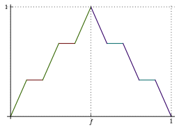
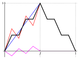
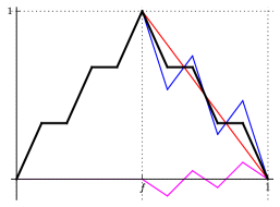
A valid function $\pi$ for $R_{\mathchoice{\mbox{\boldmath$\displaystyle\bf f$}}{\mbox{\boldmath$\textstyle\bf f$}}{\mbox{\boldmath$\scriptstyle\bf f$}}{\mbox{\boldmath$\scriptscriptstyle\bf f$}}}(G,S)$ is said to be minimal for $R_{\mathchoice{\mbox{\boldmath$\displaystyle\bf f$}}{\mbox{\boldmath$\textstyle\bf f$}}{\mbox{\boldmath$\scriptstyle\bf f$}}{\mbox{\boldmath$\scriptscriptstyle\bf f$}}}(G,S)$ if there is no valid function $\pi^{\prime}\neq\pi$ such that $\pi^{\prime}({\mathchoice{\mbox{\boldmath$\displaystyle\bf r$}}{\mbox{\boldmath$\textstyle\bf r$}}{\mbox{\boldmath$\scriptstyle\bf r$}}{\mbox{\boldmath$\scriptscriptstyle\bf r$}}})\leq\pi({\mathchoice{\mbox{\boldmath$\displaystyle\bf r$}}{\mbox{\boldmath$\textstyle\bf r$}}{\mbox{\boldmath$\scriptstyle\bf r$}}{\mbox{\boldmath$\scriptscriptstyle\bf r$}}})$ for all ${\mathchoice{\mbox{\boldmath$\displaystyle\bf r$}}{\mbox{\boldmath$\textstyle\bf r$}}{\mbox{\boldmath$\scriptstyle\bf r$}}{\mbox{\boldmath$\scriptscriptstyle\bf r$}}}\in G$. For every valid function $\pi$ for $R_{\mathchoice{\mbox{\boldmath$\displaystyle\bf f$}}{\mbox{\boldmath$\textstyle\bf f$}}{\mbox{\boldmath$\scriptstyle\bf f$}}{\mbox{\boldmath$\scriptscriptstyle\bf f$}}}(G,S)$, there exists a minimal valid function $\pi^{\prime}$ such that $\pi^{\prime}\leq\pi$ [18, Theorem 1.1], and thus non-minimal valid functions are redundant in the description of $R_{\mathchoice{\mbox{\boldmath$\displaystyle\bf f$}}{\mbox{\boldmath$\textstyle\bf f$}}{\mbox{\boldmath$\scriptstyle\bf f$}}{\mbox{\boldmath$\scriptscriptstyle\bf f$}}}(G,S)$. Note that $\pi^{\prime}$ is not uniquely determined (Figure 1).

Minimal functions for $R_{\mathchoice{\mbox{\boldmath$\displaystyle\bf f$}}{\mbox{\boldmath$\textstyle\bf f$}}{\mbox{\boldmath$\scriptstyle\bf f$}}{\mbox{\boldmath$\scriptscriptstyle\bf f$}}}(G,S)$ were characterized by Gomory for the case where $S$ has finite index in $G$ in [35], and later for $R_{\mathchoice{\mbox{\boldmath$\displaystyle\bf f$}}{\mbox{\boldmath$\textstyle\bf f$}}{\mbox{\boldmath$\scriptstyle\bf f$}}{\mbox{\boldmath$\scriptscriptstyle\bf f$}}}(\mathbb{R},\mathbb{Z})$ by Gomory and Johnson [37]. We state these results in a unified notation in the following theorem.

A function $\pi\colon G\rightarrow\mathbb{R}$ is subadditive if $\pi({\mathchoice{\mbox{\boldmath$\displaystyle\bf x$}}{\mbox{\boldmath$\textstyle\bf x$}}{\mbox{\boldmath$\scriptstyle\bf x$}}{\mbox{\boldmath$\scriptscriptstyle\bf x$}}}+{\mathchoice{\mbox{\boldmath$\displaystyle\bf y$}}{\mbox{\boldmath$\textstyle\bf y$}}{\mbox{\boldmath$\scriptstyle\bf y$}}{\mbox{\boldmath$\scriptscriptstyle\bf y$}}})\leq\pi({\mathchoice{\mbox{\boldmath$\displaystyle\bf x$}}{\mbox{\boldmath$\textstyle\bf x$}}{\mbox{\boldmath$\scriptstyle\bf x$}}{\mbox{\boldmath$\scriptscriptstyle\bf x$}}})+\pi({\mathchoice{\mbox{\boldmath$\displaystyle\bf y$}}{\mbox{\boldmath$\textstyle\bf y$}}{\mbox{\boldmath$\scriptstyle\bf y$}}{\mbox{\boldmath$\scriptscriptstyle\bf y$}}})$ for all ${\mathchoice{\mbox{\boldmath$\displaystyle\bf x$}}{\mbox{\boldmath$\textstyle\bf x$}}{\mbox{\boldmath$\scriptstyle\bf x$}}{\mbox{\boldmath$\scriptscriptstyle\bf x$}}},{\mathchoice{\mbox{\boldmath$\displaystyle\bf y$}}{\mbox{\boldmath$\textstyle\bf y$}}{\mbox{\boldmath$\scriptstyle\bf y$}}{\mbox{\boldmath$\scriptscriptstyle\bf y$}}}\in G$. We say that $\pi$ is symmetric (or satisfies the symmetry condition) if $\pi({\mathchoice{\mbox{\boldmath$\displaystyle\bf x$}}{\mbox{\boldmath$\textstyle\bf x$}}{\mbox{\boldmath$\scriptstyle\bf x$}}{\mbox{\boldmath$\scriptscriptstyle\bf x$}}})+\pi({\mathchoice{\mbox{\boldmath$\displaystyle\bf f$}}{\mbox{\boldmath$\textstyle\bf f$}}{\mbox{\boldmath$\scriptstyle\bf f$}}{\mbox{\boldmath$\scriptscriptstyle\bf f$}}}-{\mathchoice{\mbox{\boldmath$\displaystyle\bf x$}}{\mbox{\boldmath$\textstyle\bf x$}}{\mbox{\boldmath$\scriptstyle\bf x$}}{\mbox{\boldmath$\scriptscriptstyle\bf x$}}})=1$ for all ${\mathchoice{\mbox{\boldmath$\displaystyle\bf x$}}{\mbox{\boldmath$\textstyle\bf x$}}{\mbox{\boldmath$\scriptstyle\bf x$}}{\mbox{\boldmath$\scriptscriptstyle\bf x$}}}\in G$.

Theorem 2.1 (Gomory and Johnson [37]).

Let $G$ be an abelian group, $S$ be a subgroup of $G$ and ${\mathchoice{\mbox{\boldmath$\displaystyle\bf f$}}{\mbox{\boldmath$\textstyle\bf f$}}{\mbox{\boldmath$\scriptstyle\bf f$}}{\mbox{\boldmath$\scriptscriptstyle\bf f$}}}\in G\setminus S$. Let $\pi\colon G\rightarrow\mathbb{R}$ be a nonnegative function. Then $\pi$ is a minimal valid function for $R_{\mathchoice{\mbox{\boldmath$\displaystyle\bf f$}}{\mbox{\boldmath$\textstyle\bf f$}}{\mbox{\boldmath$\scriptstyle\bf f$}}{\mbox{\boldmath$\scriptscriptstyle\bf f$}}}(G,S)$ if and only if $\pi(\mathchoice{\mbox{\boldmath$\displaystyle\bf z$}}{\mbox{\boldmath$\textstyle\bf z$}}{\mbox{\boldmath$\scriptstyle\bf z$}}{\mbox{\boldmath$\scriptscriptstyle\bf z$}})=0$ for all $\mathchoice{\mbox{\boldmath$\displaystyle\bf z$}}{\mbox{\boldmath$\textstyle\bf z$}}{\mbox{\boldmath$\scriptstyle\bf z$}}{\mbox{\boldmath$\scriptscriptstyle\bf z$}}\in S$, $\pi$ is subadditive, and $\pi$ satisfies the symmetry condition. (The first two conditions imply that $\pi$ is periodic modulo $S$, that is, $\pi({\mathchoice{\mbox{\boldmath$\displaystyle\bf x$}}{\mbox{\boldmath$\textstyle\bf x$}}{\mbox{\boldmath$\scriptstyle\bf x$}}{\mbox{\boldmath$\scriptscriptstyle\bf x$}}})=\pi({\mathchoice{\mbox{\boldmath$\displaystyle\bf x$}}{\mbox{\boldmath$\textstyle\bf x$}}{\mbox{\boldmath$\scriptstyle\bf x$}}{\mbox{\boldmath$\scriptscriptstyle\bf x$}}}+\mathchoice{\mbox{\boldmath$\displaystyle\bf z$}}{\mbox{\boldmath$\textstyle\bf z$}}{\mbox{\boldmath$\scriptstyle\bf z$}}{\mbox{\boldmath$\scriptscriptstyle\bf z$}})$ for all $\mathchoice{\mbox{\boldmath$\displaystyle\bf z$}}{\mbox{\boldmath$\textstyle\bf z$}}{\mbox{\boldmath$\scriptstyle\bf z$}}{\mbox{\boldmath$\scriptscriptstyle\bf z$}}\in S$, and the symmetry condition implies that the values of minimal functions are bounded between $0$ and $1$.)

See [22, Theorem 5.4] for a proof.

Figure 3. This function (h = not_extreme_1()) is minimal, but not extreme (and hence also not a facet), as proved by extremality_test(h, show_plots=True). The procedure first shows that for any distinct minimal $\pi^{1}=\pi+\bar{\pi}$ (blue), $\pi^{2}=\pi-\bar{\pi}$ (red) such that $\pi=\tfrac{1}{2}\pi^{1}+\tfrac{1}{2}\pi^{2}$, the functions $\pi^{1}$ and $\pi^{2}$ are continuous piecewise linear with the same breakpoints as $\pi$ (in the terminology of [15], $\pi$ is affine imposing on all intervals between breakpoints). A finite-dimensional extremality test then finds two linearly independent perturbations $\bar{\pi}$ (magenta), as shown.

2.2.2. Extreme functions

In polyhedral combinatorics, one is interested in classifying the facet-defining inequalities of a polytope, which are the strongest inequalities and provide a finite minimal description. In the infinite group problem literature, three notions analogous to that of a facet-defining inequality have been proposed, which are not known to be equivalent. We start with the notion of an extreme function.

A valid function $\pi$ is extreme for $R_{\mathchoice{\mbox{\boldmath$\displaystyle\bf f$}}{\mbox{\boldmath$\textstyle\bf f$}}{\mbox{\boldmath$\scriptstyle\bf f$}}{\mbox{\boldmath$\scriptscriptstyle\bf f$}}}(G,S)$ if it cannot be written as a convex combination of two other valid functions for $R_{\mathchoice{\mbox{\boldmath$\displaystyle\bf f$}}{\mbox{\boldmath$\textstyle\bf f$}}{\mbox{\boldmath$\scriptstyle\bf f$}}{\mbox{\boldmath$\scriptscriptstyle\bf f$}}}(G,S)$, i.e., $\pi=\tfrac{1}{2}(\pi^{1}+\pi^{2})$ implies $\pi=\pi^{1}=\pi^{2}$ (see Figure 1 and Figure 3). Extreme functions are easily seen to be minimal. In fact we may view this definition from a convex geometry perspective. By Theorem 2.1, the set of minimal valid functions is a convex subset of the infinite-dimensional space $\mathbb{R}^{G}$ of real-valued functions on $G$; this follows from the observation that all the properties in Theorem 2.1 are preserved under taking convex combinations of functions.

Proposition 2.1 (New result $\clubsuit$).

The set of minimal valid functions is a compact convex set under the product topology on the space $\mathbb{R}^{G}$ of real-valued functions on $G$.

The proof appears in subsection 6.1. In the light of 2.1, it is natural to study the extreme points of this compact convex set of minimal valid functions. These are precisely the extreme functions. By an application of the Krein–Milman theorem, all minimal valid functions are either convex combinations of extreme functions or pointwise limits of such convex combinations (i.e., limits in the product topology).

2.2.3. Facets and weak facets

A related notion is that of a facet. Let $P(\pi)$ denote the set of all feasible solutions $y\in\mathbb{R}^{(G)}$ satisfying (6) such that $\sum_{r\in G}\pi(r)y(r)=1$. A valid function $\pi$ is called a facet if for every valid function $\pi^{\prime}$ such that $P(\pi)\subseteq P(\pi^{\prime})$ we have that $\pi^{\prime}=\pi$, as defined in [39]. Equivalently, a valid function $\pi$ is a facet if this condition holds for all such minimal valid functions $\pi^{\prime}$ (cf. [18]).

A similar facet definition, which we call a weak facet, is given in [26] and in fact was used in an erroneous proof of the so-called Facet Theorem in [39, Theorem 3] (see Theorem 2.2). In particular, a valid function $\pi$ is called a weak facet if for every valid function $\pi^{\prime}$ such that $P(\pi)\subseteq P(\pi^{\prime})$ we have that $P(\pi)=P(\pi^{\prime})$.

2.2.4. Relation between the three notions

Facets are extreme functions (cf. [18, Lemma 1.3]), but it is unknown if all extreme functions are facets. A facet is also a weak facet, but it is unknown if all weak facets are facets. Thus, facets are a subset of the intersection of extreme functions and weak facets, but nothing further is known in general; see Figure 2 (a). When $G$ is a finite abelian group, the set of minimal functions is a finite-dimensional polyhedron (given by constraints coming from Theorem 2.1); see subsection 8.1. In this setting, it is well known that the three notions of weak facets, facets and extreme inequalities are equivalent, and form the extreme points of this polyhedron; see Figure 2 (b). In the one-row infinite group problem, we can also establish some equivalence as stated below, which is a consequence of Theorem 8.6. The result is new and has not been published before.

Proposition 2.1 (New result $\clubsuit$).

Suppose $\pi\colon\mathbb{R}\to\mathbb{R}$ is a continuous piecewise linear function with rational breakpoints in $\frac{1}{q}\mathbb{Z}$ for some $q\in\mathbb{N}$. Then $\pi$ is extreme if and only if $\pi$ is a facet.

Open question 2.1.

Are the definitions of facets, weak facets, and extreme functions equivalent?

2.3. A roadmap for proving extremality and facetness

An understanding of the set of points for which the subadditivity relations of a minimal function hold at equality is crucial to the study of both extreme functions and facets. This motivates the following definition.

Definition 2.1.

Define the subadditivity slack of $\pi$ as

$$\Delta\pi({\mathchoice{\mbox{\boldmath$\displaystyle\bf x$}}{\mbox{\boldmath$\textstyle\bf x$}}{\mbox{\boldmath$\scriptstyle\bf x$}}{\mbox{\boldmath$\scriptscriptstyle\bf x$}}},{\mathchoice{\mbox{\boldmath$\displaystyle\bf y$}}{\mbox{\boldmath$\textstyle\bf y$}}{\mbox{\boldmath$\scriptstyle\bf y$}}{\mbox{\boldmath$\scriptscriptstyle\bf y$}}}):=\pi({\mathchoice{\mbox{\boldmath$\displaystyle\bf x$}}{\mbox{\boldmath$\textstyle\bf x$}}{\mbox{\boldmath$\scriptstyle\bf x$}}{\mbox{\boldmath$\scriptscriptstyle\bf x$}}})+\pi({\mathchoice{\mbox{\boldmath$\displaystyle\bf y$}}{\mbox{\boldmath$\textstyle\bf y$}}{\mbox{\boldmath$\scriptstyle\bf y$}}{\mbox{\boldmath$\scriptscriptstyle\bf y$}}})-\pi({\mathchoice{\mbox{\boldmath$\displaystyle\bf x$}}{\mbox{\boldmath$\textstyle\bf x$}}{\mbox{\boldmath$\scriptstyle\bf x$}}{\mbox{\boldmath$\scriptscriptstyle\bf x$}}}+{\mathchoice{\mbox{\boldmath$\displaystyle\bf y$}}{\mbox{\boldmath$\textstyle\bf y$}}{\mbox{\boldmath$\scriptstyle\bf y$}}{\mbox{\boldmath$\scriptscriptstyle\bf y$}}})$$ (7)

and the additivity domain of $\pi$ as

$$E(\pi):=\left\{\,({\mathchoice{\mbox{\boldmath$\displaystyle\bf x$}}{\mbox{\boldmath$\textstyle\bf x$}}{\mbox{\boldmath$\scriptstyle\bf x$}}{\mbox{\boldmath$\scriptscriptstyle\bf x$}}},{\mathchoice{\mbox{\boldmath$\displaystyle\bf y$}}{\mbox{\boldmath$\textstyle\bf y$}}{\mbox{\boldmath$\scriptstyle\bf y$}}{\mbox{\boldmath$\scriptscriptstyle\bf y$}}})\,\mid\,\Delta\pi({\mathchoice{\mbox{\boldmath$\displaystyle\bf x$}}{\mbox{\boldmath$\textstyle\bf x$}}{\mbox{\boldmath$\scriptstyle\bf x$}}{\mbox{\boldmath$\scriptscriptstyle\bf x$}}},{\mathchoice{\mbox{\boldmath$\displaystyle\bf y$}}{\mbox{\boldmath$\textstyle\bf y$}}{\mbox{\boldmath$\scriptstyle\bf y$}}{\mbox{\boldmath$\scriptscriptstyle\bf y$}}})=0\,\right\}.$$ (8)

Additivity domains are used by Gomory and Johnson to define the notion of merit index in [39]. The merit index is the volume of $E(\pi)$ (modulo $\mathbb{Z}^{n}$) and can be taken as a quantitative measure of strength of minimal valid functions. Work on the merit index also appears in [28]. We will not discuss the merit index in this survey; however, the set $E(\pi)$ will be crucial in what follows.

The main technique used to show a function $\pi$ is extreme is to assume that $\pi=\tfrac{1}{2}(\pi^{1}+\pi^{2})$ where $\pi^{1},\pi^{2}$ are valid functions, and then show that $\pi=\pi^{1}=\pi^{2}$. One then employs the following lemma to infer important properties of $\pi^{1},\pi^{2}$. These following facts can be found in the literature for the one-row problem; the extension to general $k$ is straightforward.

Lemma 2.1.

Let $\pi:\mathbb{R}^{k}\to\mathbb{R}_{+}$ be minimal, $\pi=\frac{1}{2}(\pi^{1}+\pi^{2})$, and $\pi^{1},\pi^{2}$ valid functions. Then the following hold:

1. $\pi^{1},\pi^{2}$ are minimal [37, Lemma 1.4].

2. All subadditivity relations $\pi({\mathchoice{\mbox{\boldmath$\displaystyle\bf x$}}{\mbox{\boldmath$\textstyle\bf x$}}{\mbox{\boldmath$\scriptstyle\bf x$}}{\mbox{\boldmath$\scriptscriptstyle\bf x$}}}+{\mathchoice{\mbox{\boldmath$\displaystyle\bf y$}}{\mbox{\boldmath$\textstyle\bf y$}}{\mbox{\boldmath$\scriptstyle\bf y$}}{\mbox{\boldmath$\scriptscriptstyle\bf y$}}})\leq\pi({\mathchoice{\mbox{\boldmath$\displaystyle\bf x$}}{\mbox{\boldmath$\textstyle\bf x$}}{\mbox{\boldmath$\scriptstyle\bf x$}}{\mbox{\boldmath$\scriptscriptstyle\bf x$}}})+\pi({\mathchoice{\mbox{\boldmath$\displaystyle\bf y$}}{\mbox{\boldmath$\textstyle\bf y$}}{\mbox{\boldmath$\scriptstyle\bf y$}}{\mbox{\boldmath$\scriptscriptstyle\bf y$}}})$ that are tight for $\pi$ are also tight for $\pi^{1},\pi^{2}$, i.e., $E(\pi)\subseteq E(\pi^{1})\cap E(\pi^{2})$ [37, proof of Theorem 3.3].

3. Suppose there exists a real number $M$ such that $\limsup_{h\to 0}\left|\frac{\pi(h{\mathchoice{\mbox{\boldmath$\displaystyle\bf r$}}{\mbox{\boldmath$\textstyle\bf r$}}{\mbox{\boldmath$\scriptstyle\bf r$}}{\mbox{\boldmath$\scriptscriptstyle\bf r$}}})}{h}\right|\leq M$ for all ${\mathchoice{\mbox{\boldmath$\displaystyle\bf r$}}{\mbox{\boldmath$\textstyle\bf r$}}{\mbox{\boldmath$\scriptstyle\bf r$}}{\mbox{\boldmath$\scriptscriptstyle\bf r$}}}\in\mathbb{R}^{k}$ such that $\lVert{\mathchoice{\mbox{\boldmath$\displaystyle\bf r$}}{\mbox{\boldmath$\textstyle\bf r$}}{\mbox{\boldmath$\scriptstyle\bf r$}}{\mbox{\boldmath$\scriptscriptstyle\bf r$}}}\rVert=1$. Then $\pi$ is Lipschitz continuous. Furthermore, this condition holds for $\pi^{1}$ and $\pi^{2}$ and $\pi^{1},\pi^{2}$ are Lipschitz continuous [15, Theorem 2.9].

4. If $\pi$ is continuous piecewise linear, then $\pi,\pi^{1},\pi^{2}$ are all Lipschitz continuous [16, LABEL:equi3:lemma:tight-implies-tight].

5. Suppose $k=1$, i.e., $\pi\colon\mathbb{R}\to\mathbb{R}_{+}$ and $\pi$ is piecewise linear and continuous from the right at $0$ or continuous from the left at $0$. Then $\pi^{1}$ and $\pi^{2}$ are continuous at all points at which $\pi$ is continuous [28, Theorem 2].

To prove that a valid inequality is a facet, the main tool is the so-called Facet Theorem, originally proved by Gomory and Johnson [39] for the one-row case; it extends verbatim to the $k$-row case. We present a stronger version of the theorem, which first appeared in [18].

Theorem 2.2 (Facet Theorem [39], [18, Theorem 3.1]).

Let $\pi$ be a minimal valid function. Suppose for every minimal valid function $\pi^{\prime}$, $E(\pi)\subseteq E(\pi^{\prime})$ implies $\pi^{\prime}=\pi$. Then $\pi$ is a facet.

In the light of 2.1 and Theorem 2.2, if one can establish that for a minimal valid function $\pi$, $E(\pi)\subseteq E(\pi^{\prime})$ implies $\pi^{\prime}=\pi$ for every minimal valid function $\pi^{\prime}$, then $\pi$ is extreme, as well as a facet. Indeed, if $\pi=\tfrac{1}{2}(\pi^{1}+\pi^{2})$ where $\pi^{1},\pi^{2}$ are valid functions, by Lemma 2.1 (i), $\pi^{1}$ and $\pi^{2}$ are minimal and by 2.1 (ii), $E(\pi)\subseteq E(\pi^{1})\cap E(\pi^{2})$, and so $\pi=\pi^{1}=\pi^{2}$. The facetness follows directly from Theorem 2.2, and gives an alternate proof of extremality since all facets are extreme.

The condition that $E(\pi)\subseteq E(\pi^{\prime})$ implies $\pi^{\prime}=\pi$ for every minimal valid function $\pi^{\prime}$ is established along the following lines. First, structural properties of $\pi$ can be used to obtain a structured description of $E(\pi)$. For example, the fact that $\pi$ is piecewise linear often shows that $E(\pi)$ is the union of many full-dimensional convex sets. $E(\pi^{\prime})$ shares this structure with $E(\pi)$ because of the assumption that $E(\pi)\subseteq E(\pi^{\prime})$. Then, results such as the Interval Lemma, discussed in section 4, are used to show that $\pi^{\prime}$ must be affine on the set of points contributing to $E(\pi^{\prime})$. Finally, the conditions that all minimal valid functions are $0$ at the origin and $1$ at ${\mathchoice{\mbox{\boldmath$\displaystyle\bf f$}}{\mbox{\boldmath$\textstyle\bf f$}}{\mbox{\boldmath$\scriptstyle\bf f$}}{\mbox{\boldmath$\scriptscriptstyle\bf f$}}}+\mathbb{Z}^{k}$ puts further restrictions on the values that $\pi^{\prime}$ can take, and ultimately force $\pi^{\prime}=\pi$.

2.4. Classification and taxonomy of facets and extreme functions

The main goal in the study of the infinite group problem is to obtain a classification of facets and extreme valid functions. We do not believe that a simple classification exists like Theorem 2.1 for minimal valid functions. In spite of this, several beautiful theorems have been obtained regarding the structure of facets and extreme valid functions, and there is a lot more to be discovered. This survey attempts to highlight the most important known results in this research area and outline some of the challenging open problems.

Inspired by the survey by Richard and Dey [48, p. 786], we provide an updated compendium, or “taxonomy,” of known extreme functions at the end of this survey (Appendix A). The focus lies on the case of the one-row ($k=1$) infinite group problem, $R_{f}(\mathbb{R},\mathbb{Z})$, for which many types of extreme functions have been discovered and analyzed (Table 1, 2, 3, 4). Also a number of “procedures” (operations) have been studied in the literature that preserve extremality under some conditions; we present these in Table 5.

We do not provide explicit constructions or descriptions of these functions here. Instead, we invite the interested reader to investigate the functions in an interactive companion program [41], including the electronic compendium of extreme functions [51]. The program and the electronic compendium are implemented in the free (open-source) computer algebra package Sage [50].

Most facets and extreme functions described in the literature are piecewise linear functions. The number of slopes (i.e., the different values of the derivative) of a function is a statistic that has received much attention in the literature. In fact, one of the classic results in the study of extreme functions for the single-row problem is the following:

Theorem 2.3 (Gomory–Johnson 2-Slope Theorem [37]).

If a continuous piecewise linear minimal function of $R_{f}(\mathbb{R},\mathbb{Z})$ has only 2 values for the derivative wherever it exists (2 slopes), then the function is extreme.

Among the types of extreme functions that are piecewise linear functions, there are discontinuous and continuous ones. In the single-row case ($k=1$), continuous piecewise linear extreme functions with 2, 3 and 4 different slopes were previously known, and discontinuous piecewise linear extreme functions with 1 and 2 slopes were previously known. Moreover, all previously known examples of extreme discontinuous functions were continuous on one side of the origin. Hildebrand (2013, unpublished) found continuous piecewise linear extreme functions with 5 slopes using computer-based search, as well as various discontinuous piecewise linear extreme functions. Köppe and Zhou [46] later found continuous piecewise linear extreme functions with up to 28 slopes.

Proposition 2.3 (New result $\clubsuit$).

There exist continuous piecewise linear extreme functions with 5, 6, 7, and 28 slopes. There exist discontinuous piecewise linear extreme functions with 3 slopes and discontinuous piecewise linear extreme functions that are discontinuous on both sides at the origin. See Table 4.

This prompts the following question.

Open question 2.3.

For the single-row problem $R_{f}(\mathbb{R},\mathbb{Z})$, do there exist continuous and discontinuous extreme functions with $s$ slopes for every $s\geq 2$?

The additivity domain $E(\pi)$ for any minimal function $\pi$ (see (8)) can be decomposed as the union of its maximal convex subsets. The first 5-slope functions found by Hildebrand (2013) have an additivity domain which contains lower-dimensional maximal convex components. This begs the question:

Open question 2.3.

For the single-row problem $R_{f}(\mathbb{R},\mathbb{Z})$, do there exist continuous piecewise linear extreme functions of $R_{f}(\mathbb{R},\mathbb{Z})$ with $s$ slopes such that $E(\pi)$ is the union of full-dimensional convex sets for every $s\geq 2$?

Not all facets and extreme functions are piecewise linear though. Basu, Conforti, Cornuéjols, and Zambelli [12] constructed a family of facets that are not piecewise linear, yet the derivatives (where they exist) only take 2 values; see subsection 6.4. A function $\tilde{\pi}$ from this family is absolutely continuous and therefore it is differentiable almost everywhere (a.e.). The derivative $\tilde{\pi}^{\prime}$ happens to take only two different values a.e., so $\tilde{\pi}$ is a “generalized 2-slope function.” This suggests the following refined version of Gomory and Johnson’s original piecewise linear conjecture for extreme functions.

Conjecture 2.3.

For every absolutely continuous extreme function $\pi\colon\mathbb{R}\to\mathbb{R}$, the derivative $\pi^{\prime}$ is a simple function. Thus, there exists a finite partition of $\mathbb{R}$ into measureable subsets $M_{0},\ldots,M_{t}$ such that $M_{0}$ is of measure zero and $\pi^{\prime}$ is constant over each of $M_{1},\ldots,M_{t}$.

The fact that the derivative of the counterexample from [12] happens to take only two different values a.e. also gives rise to the following generalized 2-slope conjecture. This conjecture would generalize Theorem 2.3.

Conjecture 2.3.

Let $\pi\colon\mathbb{R}\rightarrow\mathbb{R}$ be a minimal function that is absolutely continuous and whose derivative $\pi^{\prime}$ only takes two values outside of a set of measure zero. Then $\pi$ is extreme.

The key difficulty in answering the above questions is that the tools of functional equations (such as the Interval Lemma as discussed in section 4) no longer directly apply and new tools will most likely need to be employed for the resolution. Thus, there are still substantial questions left to be explored, even for the single-row ($k=1$) problem.

Much less is known about the $k$-row problem $R_{\mathchoice{\mbox{\boldmath$\displaystyle\bf f$}}{\mbox{\boldmath$\textstyle\bf f$}}{\mbox{\boldmath$\scriptstyle\bf f$}}{\mbox{\boldmath$\scriptscriptstyle\bf f$}}}(\mathbb{R}^{k},\mathbb{Z}^{k})$ for general $k$. Dey and Richard [27] pioneered the construction of extreme functions for the $k$-row problem. Their sequential-merge procedure constructs extreme functions and facets for $k\geq 2$ dimensions by combining extreme functions and facets for smaller $k$; see subsection 5.2. As mentioned earlier, a breakthrough was made when Theorem 5.1 was proved in [18, Theorem 1.7], generalizing Gomory and Johnson’s single-row result (Theorem 2.3) to the general $k$-row problem, giving a very general sufficient condition for extremality and facetness.

3. The $k$-dimensional theory of piecewise linear minimal valid functions

3.1. Polyhedral complexes and piecewise linear functions

We introduce the notion of polyhedral complexes, which serves two purposes. First, it provides a framework to define piecewise linear functions, generalizing the familiar situation of functions of a single real variable. Second it is a tool for studying subadditivity and additivity relations of these functions. This exposition follows [16].

Definition 3.0.

A (locally finite) polyhedral complex is a collection $\mathcal{P}$ of polyhedra in $\mathbb{R}^{k}$ such that:

1. $\emptyset\in\mathcal{P}$,

2. if $I\in\mathcal{P}$, then all faces of $I$ are in $\mathcal{P}$,

3. the intersection $I\cap J$ of two polyhedra $I,J\in\mathcal{P}$ is a face of both $I$ and $J$,

4. any compact subset of $\mathbb{R}^{k}$ intersects only finitely many faces in $\mathcal{P}$.

A polyhedron $I$ from $\mathcal{P}$ is called a face of the complex. A polyhedral complex $\mathcal{P}$ is said to be pure if all its maximal faces (with respect to set inclusion) have the same dimension. In this case, we call the maximal faces of $\mathcal{P}$ the cells of $\mathcal{P}$. The zero-dimensional faces of $\mathcal{P}$ are called vertices and the set of vertices of $\mathcal{P}$ will be denoted by $\operatorname{vert}(\mathcal{P})$. A polyhedral complex $\mathcal{P}$ is said to be complete if the union of all faces of the complex is $\mathbb{R}^{k}$. A pure and complete polyhedral complex $\mathcal{P}$ is called a triangulation of $\mathbb{R}^{k}$ if every maximal cell is a simplex.

Example 3.0 (Breakpoint intervals in $\mathbf{R}^{1}$ [15]).

Let $0=x_{0}<x_{1}<\dots<x_{n-1}<x_{n}=1$ be a list of “breakpoints” in $[0,1]$. We extend it periodically as $B=\{\,x_{0}+t,x_{1}+t,\dots,x_{n-1}+t\mid t\in\mathbb{Z}\,\}$. Define the set of 0-dimensional faces to be the collection of singletons, $\mathcal{P}_{B,{\text{\leavevmode\hbox{\set@color \leavevmode\hbox to1.81pt{\vbox to1.81pt{\pgfpicture\makeatletter\hbox{\hskip 0.90417pt\lower 1.20555pt\hbox to0.0pt{\pgfsys@beginscope\pgfsys@invoke{ }\definecolor{pgfstrokecolor}{rgb}{0,0,0}\pgfsys@color@rgb@stroke{0}{0}{0}\pgfsys@invoke{ }\pgfsys@color@rgb@fill{0}{0}{0}\pgfsys@invoke{ }\pgfsys@setlinewidth{0.4pt}\pgfsys@invoke{ }\nullfont\hbox to0.0pt{\pgfsys@beginscope\pgfsys@invoke{ }{}{ {{}{}}{{}}{}{{{}}{}{}{}{}{}{}{}{}}\pgfsys@moveto{0.0pt}{2.10973pt}\pgfsys@moveto{0.90417pt}{2.10973pt}\pgfsys@curveto{0.90417pt}{2.60909pt}{0.49936pt}{3.0139pt}{0.0pt}{3.0139pt}\pgfsys@curveto{-0.49936pt}{3.0139pt}{-0.90417pt}{2.60909pt}{-0.90417pt}{2.10973pt}\pgfsys@curveto{-0.90417pt}{1.61037pt}{-0.49936pt}{1.20555pt}{0.0pt}{1.20555pt}\pgfsys@curveto{0.49936pt}{1.20555pt}{0.90417pt}{1.61037pt}{0.90417pt}{2.10973pt}\pgfsys@closepath\pgfsys@moveto{0.0pt}{2.10973pt}\pgfsys@fill\pgfsys@invoke{ } } \pgfsys@invoke{\lxSVG@closescope }\pgfsys@endscope{}{}{}\hss}\pgfsys@discardpath\pgfsys@invoke{\lxSVG@closescope }\pgfsys@endscope\hss}}\lxSVG@closescope\endpgfpicture}}}}}}=\bigl{\{}\,\{x\}\mid x\in B\,\bigr{\}},$ and the set of one-dimensional faces to be the collection of closed intervals, $\mathcal{P}_{B,{\text{\leavevmode\hbox{\set@color \leavevmode\hbox to6.97pt{\vbox to3.99pt{\pgfpicture\makeatletter\hbox{\hskip 0.53798pt\lower-1.48195pt\hbox to0.0pt{\pgfsys@beginscope\pgfsys@invoke{ }\definecolor{pgfstrokecolor}{rgb}{0,0,0}\pgfsys@color@rgb@stroke{0}{0}{0}\pgfsys@invoke{ }\pgfsys@color@rgb@fill{0}{0}{0}\pgfsys@invoke{ }\pgfsys@setlinewidth{0.4pt}\pgfsys@invoke{ }\nullfont\hbox to0.0pt{\pgfsys@beginscope\pgfsys@invoke{ }{}{ {{}{}}{{}}{} {}{}\pgfsys@beginscope\pgfsys@invoke{ }\pgfsys@setlinewidth{0.8pt}\pgfsys@invoke{ }{}{{ {\pgfsys@beginscope{{}} {} {}{}{} {} {}{}{} {} {}{}{} \pgfsys@moveto{-0.53798pt}{0.4pt}\pgfsys@curveto{-0.25299pt}{0.4pt}{-0.25299pt}{0.56pt}{-0.25299pt}{1.48195pt}\pgfsys@lineto{0.032pt}{1.48195pt}\pgfsys@curveto{0.00002pt}{0.37999pt}{0.00002pt}{-0.37999pt}{0.032pt}{-1.48195pt}\pgfsys@lineto{-0.25299pt}{-1.48195pt}\pgfsys@curveto{-0.25299pt}{-0.56pt}{-0.25299pt}{-0.4pt}{-0.53798pt}{-0.4pt}\pgfsys@closepath\pgfsys@fill\pgfsys@endscope}} }{}{}{{}}{}{}{}{{}}\pgfsys@moveto{0.03198pt}{2.10973pt}\pgfsys@lineto{5.99579pt}{2.10973pt}\pgfsys@stroke\pgfsys@invoke{ }{{}{{}}{}{}{{}}{{{}}{{{}}{\pgfsys@beginscope\pgfsys@invoke{ }\pgfsys@transformcm{-1.0}{0.0}{0.0}{-1.0}{0.03198pt}{2.10973pt}\pgfsys@invoke{ }\pgfsys@invoke{ \lxSVG@closescope }\pgfsys@invoke{\lxSVG@closescope }\pgfsys@endscope}}{{}}}}{{}{{}}{}{}{{}}{{{}}{{{}}{\pgfsys@beginscope\pgfsys@invoke{ }\pgfsys@transformcm{1.0}{0.0}{0.0}{1.0}{5.99579pt}{2.10973pt}\pgfsys@invoke{ }\pgfsys@invoke{ \lxSVG@closescope }\pgfsys@invoke{\lxSVG@closescope }\pgfsys@endscope}}{{}}}} \pgfsys@invoke{\lxSVG@closescope }\pgfsys@endscope} \pgfsys@invoke{\lxSVG@closescope }\pgfsys@endscope{}{}{}\hss}\pgfsys@discardpath\pgfsys@invoke{\lxSVG@closescope }\pgfsys@endscope\hss}}\lxSVG@closescope\endpgfpicture}}}}}}=\bigl{\{}\,[x_{i}+t,x_{i+1}+t]\mid i=0,\dots,{n-1}\text{ and }t\in\mathbb{Z}\,\bigr{\}}.$ Then $\mathcal{P}_{B}=\{\emptyset\}\cup\mathcal{P}_{B,{\text{\leavevmode}}}\cup\mathcal{P}_{B,{\text{\leavevmode}}}$ is a locally finite polyhedral complex.

Example 3.0 (Standard triangulations of $\mathbf{R}^{2}$ [16]).

Let $q$ be a positive integer. Consider the arrangement $\mathcal{H}_{q}$ of all hyperplanes (lines) of $\mathbb{R}^{2}$ of the form ${\bigl{(}\begin{smallmatrix}0\vphantom{/}\\ 1\vphantom{/}\end{smallmatrix}\bigr{)}}\cdot{\mathchoice{\mbox{\boldmath$\displaystyle\bf x$}}{\mbox{\boldmath$\textstyle\bf x$}}{\mbox{\boldmath$\scriptstyle\bf x$}}{\mbox{\boldmath$\scriptscriptstyle\bf x$}}}=b$, ${\bigl{(}\begin{smallmatrix}1\vphantom{/}\\ 0\vphantom{/}\end{smallmatrix}\bigr{)}}\cdot{\mathchoice{\mbox{\boldmath$\displaystyle\bf x$}}{\mbox{\boldmath$\textstyle\bf x$}}{\mbox{\boldmath$\scriptstyle\bf x$}}{\mbox{\boldmath$\scriptscriptstyle\bf x$}}}=b$, and ${\bigl{(}\begin{smallmatrix}1\vphantom{/}\\ 1\vphantom{/}\end{smallmatrix}\bigr{)}}\cdot{\mathchoice{\mbox{\boldmath$\displaystyle\bf x$}}{\mbox{\boldmath$\textstyle\bf x$}}{\mbox{\boldmath$\scriptstyle\bf x$}}{\mbox{\boldmath$\scriptscriptstyle\bf x$}}}=b$, where $b\in\tfrac{1}{q}\mathbb{Z}$. The complement of the arrangement $\mathcal{H}_{q}$ consists of two-dimensional cells, whose closures are the triangles

$${}_{\mathchoice{\mbox{\boldmath$\displaystyle\bf 0$}}{\mbox{\boldmath$\textstyle\bf 0$}}{\mbox{\boldmath$\scriptstyle\bf 0$}}{\mbox{\boldmath$\scriptscriptstyle\bf 0$}}}{\text{\leavevmode\hbox{\set@color \leavevmode\hbox to9.01pt{\vbox to9.01pt{\pgfpicture\makeatletter\hbox{\hskip 0.2pt\lower-1.49165pt\hbox to0.0pt{\pgfsys@beginscope\pgfsys@invoke{ }\definecolor{pgfstrokecolor}{rgb}{0,0,0}\pgfsys@color@rgb@stroke{0}{0}{0}\pgfsys@invoke{ }\pgfsys@color@rgb@fill{0}{0}{0}\pgfsys@invoke{ }\pgfsys@setlinewidth{0.4pt}\pgfsys@invoke{ }\nullfont\hbox to0.0pt{\pgfsys@beginscope\pgfsys@invoke{ }{}{ {{}{}}{{}}{} {}{{}}{}{}{}{}{{}}{}\pgfsys@beginscope\pgfsys@invoke{ }\pgfsys@setdash{0.4pt,1.0pt}{0.0pt}\pgfsys@invoke{ }{}\pgfsys@moveto{0.0pt}{-1.29166pt}\pgfsys@moveto{0.0pt}{-1.29166pt}\pgfsys@lineto{0.0pt}{7.31943pt}\pgfsys@lineto{8.61108pt}{7.31943pt}\pgfsys@lineto{8.61108pt}{-1.29166pt}\pgfsys@closepath\pgfsys@moveto{8.61108pt}{7.31943pt}\pgfsys@stroke\pgfsys@invoke{ } \pgfsys@invoke{\lxSVG@closescope }\pgfsys@endscope{{}{}}{{}}{} {{}{}}{} {}{} {}\pgfsys@beginscope\pgfsys@invoke{ }\color[rgb]{0.7,0.7,0.7}\definecolor[named]{pgfstrokecolor}{rgb}{0.7,0.7,0.7}\pgfsys@color@gray@stroke{0.7}\pgfsys@invoke{ }\pgfsys@color@gray@fill{0.7}\pgfsys@invoke{ }\definecolor{pgffillcolor}{rgb}{0.7,0.7,0.7}\definecolor[named]{pgfstrokecolor}{rgb}{0,0,0}\pgfsys@color@gray@stroke{0}\pgfsys@invoke{ }{}\pgfsys@moveto{0.0pt}{-1.29166pt}\pgfsys@lineto{0.0pt}{7.31943pt}\pgfsys@lineto{8.61108pt}{-1.29166pt}\pgfsys@closepath\pgfsys@fillstroke\pgfsys@invoke{ } \pgfsys@invoke{\lxSVG@closescope }\pgfsys@endscope} \pgfsys@invoke{\lxSVG@closescope }\pgfsys@endscope{}{}{}\hss}\pgfsys@discardpath\pgfsys@invoke{\lxSVG@closescope }\pgfsys@endscope\hss}}\lxSVG@closescope\endpgfpicture}}}}}=\tfrac{1}{q}\operatorname{conv}(\{{\bigl{(}\begin{smallmatrix}0\vphantom{/}\\ 0\vphantom{/}\end{smallmatrix}\bigr{)}},{\bigl{(}\begin{smallmatrix}1\vphantom{/}\\ 0\vphantom{/}\end{smallmatrix}\bigr{)}},{\bigl{(}\begin{smallmatrix}0\vphantom{/}\\ 1\vphantom{/}\end{smallmatrix}\bigr{)}}\})\qquad\text{and}\qquad_{\mathchoice{\mbox{\boldmath$\displaystyle\bf 0$}}{\mbox{\boldmath$\textstyle\bf 0$}}{\mbox{\boldmath$\scriptstyle\bf 0$}}{\mbox{\boldmath$\scriptscriptstyle\bf 0$}}}{\text{\leavevmode\hbox{\set@color \leavevmode\hbox to9.01pt{\vbox to9.01pt{\pgfpicture\makeatletter\hbox{\hskip 0.2pt\lower-1.49165pt\hbox to0.0pt{\pgfsys@beginscope\pgfsys@invoke{ }\definecolor{pgfstrokecolor}{rgb}{0,0,0}\pgfsys@color@rgb@stroke{0}{0}{0}\pgfsys@invoke{ }\pgfsys@color@rgb@fill{0}{0}{0}\pgfsys@invoke{ }\pgfsys@setlinewidth{0.4pt}\pgfsys@invoke{ }\nullfont\hbox to0.0pt{\pgfsys@beginscope\pgfsys@invoke{ }{}{ {{}{}}{{}}{} {}{{}}{}{}{}{}{{}}{}\pgfsys@beginscope\pgfsys@invoke{ }\pgfsys@setdash{0.4pt,1.0pt}{0.0pt}\pgfsys@invoke{ }{}\pgfsys@moveto{0.0pt}{-1.29166pt}\pgfsys@moveto{0.0pt}{-1.29166pt}\pgfsys@lineto{0.0pt}{7.31943pt}\pgfsys@lineto{8.61108pt}{7.31943pt}\pgfsys@lineto{8.61108pt}{-1.29166pt}\pgfsys@closepath\pgfsys@moveto{8.61108pt}{7.31943pt}\pgfsys@stroke\pgfsys@invoke{ } \pgfsys@invoke{\lxSVG@closescope }\pgfsys@endscope{}{{}}{} {{}{}}{} {}{} {}\pgfsys@beginscope\pgfsys@invoke{ }\color[rgb]{0.7,0.7,0.7}\definecolor[named]{pgfstrokecolor}{rgb}{0.7,0.7,0.7}\pgfsys@color@gray@stroke{0.7}\pgfsys@invoke{ }\pgfsys@color@gray@fill{0.7}\pgfsys@invoke{ }\definecolor{pgffillcolor}{rgb}{0.7,0.7,0.7}\definecolor[named]{pgfstrokecolor}{rgb}{0,0,0}\pgfsys@color@gray@stroke{0}\pgfsys@invoke{ }{}\pgfsys@moveto{8.61108pt}{7.31943pt}\pgfsys@lineto{0.0pt}{7.31943pt}\pgfsys@lineto{8.61108pt}{-1.29166pt}\pgfsys@closepath\pgfsys@fillstroke\pgfsys@invoke{ } \pgfsys@invoke{\lxSVG@closescope }\pgfsys@endscope} \pgfsys@invoke{\lxSVG@closescope }\pgfsys@endscope{}{}{}\hss}\pgfsys@discardpath\pgfsys@invoke{\lxSVG@closescope }\pgfsys@endscope\hss}}\lxSVG@closescope\endpgfpicture}}}}}=\tfrac{1}{q}\operatorname{conv}(\{{\bigl{(}\begin{smallmatrix}1\vphantom{/}\\ 0\vphantom{/}\end{smallmatrix}\bigr{)}},{\bigl{(}\begin{smallmatrix}0\vphantom{/}\\ 1\vphantom{/}\end{smallmatrix}\bigr{)}},{\bigl{(}\begin{smallmatrix}1\vphantom{/}\\ 1\vphantom{/}\end{smallmatrix}\bigr{)}}\})$$

and their translates by elements of the lattice $\smash[t]{\frac{1}{q}\mathbb{Z}^{2}}$. We denote by $\mathcal{P}_{q}$ the collection of these triangles and the vertices and edges that arise as intersections of the triangles, and the empty set. Thus $\mathcal{P}_{q}$ is a locally finite polyhedral complex. Since all nonempty faces of $\mathcal{P}_{q}$ are simplices, it is a triangulation of the space $\mathbb{R}^{2}$.

We give a precise definition of affine linear functions over a domain, suitable for the general $k$-dimensional case.

Definition 3.0.

Let $U\subseteq\mathbb{R}^{k}$. We say $\pi\colon U\to\mathbb{R}$ is affine (or affine linear) over $U$ if there exists a gradient ${\mathchoice{\mbox{\boldmath$\displaystyle\bf c$}}{\mbox{\boldmath$\textstyle\bf c$}}{\mbox{\boldmath$\scriptstyle\bf c$}}{\mbox{\boldmath$\scriptscriptstyle\bf c$}}}\in\mathbb{R}^{k}$ such that for any ${\mathchoice{\mbox{\boldmath$\displaystyle\bf u$}}{\mbox{\boldmath$\textstyle\bf u$}}{\mbox{\boldmath$\scriptstyle\bf u$}}{\mbox{\boldmath$\scriptscriptstyle\bf u$}}}_{1},{\mathchoice{\mbox{\boldmath$\displaystyle\bf u$}}{\mbox{\boldmath$\textstyle\bf u$}}{\mbox{\boldmath$\scriptstyle\bf u$}}{\mbox{\boldmath$\scriptscriptstyle\bf u$}}}_{2}\in U$ we have

$$\pi({\mathchoice{\mbox{\boldmath$\displaystyle\bf u$}}{\mbox{\boldmath$\textstyle\bf u$}}{\mbox{\boldmath$\scriptstyle\bf u$}}{\mbox{\boldmath$\scriptscriptstyle\bf u$}}}_{2})-\pi({\mathchoice{\mbox{\boldmath$\displaystyle\bf u$}}{\mbox{\boldmath$\textstyle\bf u$}}{\mbox{\boldmath$\scriptstyle\bf u$}}{\mbox{\boldmath$\scriptscriptstyle\bf u$}}}_{1})={\mathchoice{\mbox{\boldmath$\displaystyle\bf c$}}{\mbox{\boldmath$\textstyle\bf c$}}{\mbox{\boldmath$\scriptstyle\bf c$}}{\mbox{\boldmath$\scriptscriptstyle\bf c$}}}\cdot({\mathchoice{\mbox{\boldmath$\displaystyle\bf u$}}{\mbox{\boldmath$\textstyle\bf u$}}{\mbox{\boldmath$\scriptstyle\bf u$}}{\mbox{\boldmath$\scriptscriptstyle\bf u$}}}_{2}-{\mathchoice{\mbox{\boldmath$\displaystyle\bf u$}}{\mbox{\boldmath$\textstyle\bf u$}}{\mbox{\boldmath$\scriptstyle\bf u$}}{\mbox{\boldmath$\scriptscriptstyle\bf u$}}}_{1}).$$

Given a pure and complete polyhedral complex $\mathcal{P}$, we call a function $\pi\colon\mathbb{R}^{k}\to\mathbb{R}$ piecewise linear over $\mathcal{P}$ if it is affine linear over the relative interior of each face of the complex. Under this definition, piecewise linear functions can be discontinuous. We say the function $\pi$ is continuous piecewise linear over $\mathcal{P}$ if it is affine over each of the cells of $\mathcal{P}$ (thus automatically imposing continuity). Most of the results presented in this survey will be about continuous piecewise linear functions.

Motivated by Gomory–Johnson’s characterization of minimal valid functions (Theorem 2.1), we are interested in functions $\pi\colon\mathbb{R}^{k}\to\mathbb{R}$ that are periodic modulo $\mathbb{Z}^{k}$, i.e., for all $\mathchoice{\mbox{\boldmath$\displaystyle\bf x$}}{\mbox{\boldmath$\textstyle\bf x$}}{\mbox{\boldmath$\scriptstyle\bf x$}}{\mbox{\boldmath$\scriptscriptstyle\bf x$}}\in\mathbb{R}^{k}$ and all vectors $\mathchoice{\mbox{\boldmath$\displaystyle\bf t$}}{\mbox{\boldmath$\textstyle\bf t$}}{\mbox{\boldmath$\scriptstyle\bf t$}}{\mbox{\boldmath$\scriptscriptstyle\bf t$}}\in\mathbb{Z}^{k}$, we have $\pi(\mathchoice{\mbox{\boldmath$\displaystyle\bf x$}}{\mbox{\boldmath$\textstyle\bf x$}}{\mbox{\boldmath$\scriptstyle\bf x$}}{\mbox{\boldmath$\scriptscriptstyle\bf x$}}+\mathchoice{\mbox{\boldmath$\displaystyle\bf t$}}{\mbox{\boldmath$\textstyle\bf t$}}{\mbox{\boldmath$\scriptstyle\bf t$}}{\mbox{\boldmath$\scriptscriptstyle\bf t$}})=\pi(\mathchoice{\mbox{\boldmath$\displaystyle\bf x$}}{\mbox{\boldmath$\textstyle\bf x$}}{\mbox{\boldmath$\scriptstyle\bf x$}}{\mbox{\boldmath$\scriptscriptstyle\bf x$}})$. If $\pi$ is periodic modulo $\mathbb{Z}^{k}$ and continuous piecewise linear over a pure and complete complex $\mathcal{P}$, then we can assume without loss of generality that $\mathcal{P}$ is also periodic modulo $\mathbb{Z}^{k}$, i.e., for all $I\in\mathcal{P}$ and all vectors $\mathchoice{\mbox{\boldmath$\displaystyle\bf t$}}{\mbox{\boldmath$\textstyle\bf t$}}{\mbox{\boldmath$\scriptstyle\bf t$}}{\mbox{\boldmath$\scriptscriptstyle\bf t$}}\in\mathbb{Z}^{k}$, the translated polyhedron $I+\mathchoice{\mbox{\boldmath$\displaystyle\bf t$}}{\mbox{\boldmath$\textstyle\bf t$}}{\mbox{\boldmath$\scriptstyle\bf t$}}{\mbox{\boldmath$\scriptscriptstyle\bf t$}}$ also is a face of $\mathcal{P}$. This is the case in Examples 3.0 and 3.0.

Remark 3.0.

If all the cells of the polyhedral complex are bounded, the value of a continuous piecewise linear function at any point $\textstyle\bf x$ can be obtained by interpolating the values of the function at the vertices of the minimal face containing $\textstyle\bf x$. This is utilized in subsection 8.2. The assumption of boundedness of the cells can be made without loss of generality; see subsection 3.3. Moreover, for a periodic continuous piecewise linear function over a periodic complex, we can give a finite description for $\pi$ by further restricting to the values in $\operatorname{vert}(\mathcal{P})\cap D$ where $D=[0,1]^{k}$ or any set such that $D+\mathbb{Z}^{k}=\mathbb{R}^{k}$. The finiteness of the set $\operatorname{vert}(\mathcal{P})\cap D$ is guaranteed by the assumption of local finiteness in 3.0 (iv).

3.2. The extended complex $\Delta\mathcal{P}$

For any $I,J,K\subseteq\mathbb{R}^{k}$, we define the set

$$F(I,J,K)=\left\{\,({\mathchoice{\mbox{\boldmath$\displaystyle\bf x$}}{\mbox{\boldmath$\textstyle\bf x$}}{\mbox{\boldmath$\scriptstyle\bf x$}}{\mbox{\boldmath$\scriptscriptstyle\bf x$}}},{\mathchoice{\mbox{\boldmath$\displaystyle\bf y$}}{\mbox{\boldmath$\textstyle\bf y$}}{\mbox{\boldmath$\scriptstyle\bf y$}}{\mbox{\boldmath$\scriptscriptstyle\bf y$}}})\in\mathbb{R}^{k}\times\mathbb{R}^{k}\,\mid\,{\mathchoice{\mbox{\boldmath$\displaystyle\bf x$}}{\mbox{\boldmath$\textstyle\bf x$}}{\mbox{\boldmath$\scriptstyle\bf x$}}{\mbox{\boldmath$\scriptscriptstyle\bf x$}}}\in I,\,{\mathchoice{\mbox{\boldmath$\displaystyle\bf y$}}{\mbox{\boldmath$\textstyle\bf y$}}{\mbox{\boldmath$\scriptstyle\bf y$}}{\mbox{\boldmath$\scriptscriptstyle\bf y$}}}\in J,\,{\mathchoice{\mbox{\boldmath$\displaystyle\bf x$}}{\mbox{\boldmath$\textstyle\bf x$}}{\mbox{\boldmath$\scriptstyle\bf x$}}{\mbox{\boldmath$\scriptscriptstyle\bf x$}}}+{\mathchoice{\mbox{\boldmath$\displaystyle\bf y$}}{\mbox{\boldmath$\textstyle\bf y$}}{\mbox{\boldmath$\scriptstyle\bf y$}}{\mbox{\boldmath$\scriptscriptstyle\bf y$}}}\in K\,\right\}.$$ (9)

When $I,J,K$ are polyhedra, $F(I,J,K)$ is also a polyhedron. Let $\mathcal{P}$ be a pure, complete polyhedral complex of $\mathbb{R}^{k}$ and let $\pi$ be a continuous piecewise linear function over $\mathcal{P}$. In order to study the additivity domain $E(\pi)$, we define the family of polyhedra in $\mathbb{R}^{k}\times\mathbb{R}^{k}$,

$$\Delta\mathcal{P}=\left\{\,F(I,J,K)\,\mid\,I,J,K\in\mathcal{P}\,\right\},$$

which is also polyhedral complex [16, LABEL:equi3:lemma:delta-p-is-complex]; see Figure 4.

Figure 4. Two diagrams of a function (blue graphs on the top and the left) and its polyhedral complex $\Delta\mathcal{P}$ (gray solid lines), as plotted by the command plot_2d_diagram(h). Left, h = gj_forward_3_slope() (left). Right, h = not_minimal_2(). The set $E(\pi)$ in both cases is the union of the faces shaded in green. The heavy diagonal green line $x+y=f$ corresponds to the symmetry condition. Vertices of $\Delta\mathcal{P}$ do not necessarily project (dotted gray lines) to breakpoints; compare with Figure 7. Vertices of the complex on which $\Delta\pi<0$, i.e., subadditivity is violated, are shown as red dots; see Theorem 3.2. At the borders of each diagram, the projections $p_{i}(F)$ of two-dimensional additive faces are shown as gray shadows: $p_{1}(F)$ at the top border, $p_{2}(F)$ at the left border, $p_{3}(F)$ at the bottom and the right borders.

Figure 5. A face $F=F(I,J,K)$ and its projections $I^{\prime}=p_{1}(F)$, $J^{\prime}=p_{2}(F)$, $K^{\prime}=p_{3}(F)$. This is an abstract picture; note that if $I^{\prime},J^{\prime},K^{\prime}\subseteq\mathbb{R}^{2}$ are full-dimensional, then $F(I,J,K)$ is actually a full-dimensional set of $\mathbb{R}^{4}$.

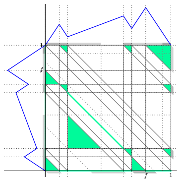
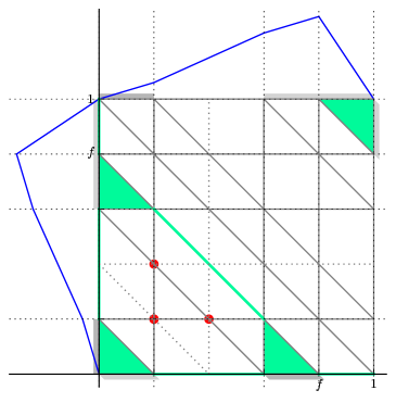
Define the projections $p_{1},p_{2},p_{3}\colon\mathbb{R}^{k}\times\mathbb{R}^{k}\to\mathbb{R}^{k}$ as

$$p_{1}({\mathchoice{\mbox{\boldmath$\displaystyle\bf x$}}{\mbox{\boldmath$\textstyle\bf x$}}{\mbox{\boldmath$\scriptstyle\bf x$}}{\mbox{\boldmath$\scriptscriptstyle\bf x$}}},{\mathchoice{\mbox{\boldmath$\displaystyle\bf y$}}{\mbox{\boldmath$\textstyle\bf y$}}{\mbox{\boldmath$\scriptstyle\bf y$}}{\mbox{\boldmath$\scriptscriptstyle\bf y$}}})={\mathchoice{\mbox{\boldmath$\displaystyle\bf x$}}{\mbox{\boldmath$\textstyle\bf x$}}{\mbox{\boldmath$\scriptstyle\bf x$}}{\mbox{\boldmath$\scriptscriptstyle\bf x$}}},\quad p_{2}({\mathchoice{\mbox{\boldmath$\displaystyle\bf x$}}{\mbox{\boldmath$\textstyle\bf x$}}{\mbox{\boldmath$\scriptstyle\bf x$}}{\mbox{\boldmath$\scriptscriptstyle\bf x$}}},{\mathchoice{\mbox{\boldmath$\displaystyle\bf y$}}{\mbox{\boldmath$\textstyle\bf y$}}{\mbox{\boldmath$\scriptstyle\bf y$}}{\mbox{\boldmath$\scriptscriptstyle\bf y$}}})={\mathchoice{\mbox{\boldmath$\displaystyle\bf y$}}{\mbox{\boldmath$\textstyle\bf y$}}{\mbox{\boldmath$\scriptstyle\bf y$}}{\mbox{\boldmath$\scriptscriptstyle\bf y$}}},\quad p_{3}({\mathchoice{\mbox{\boldmath$\displaystyle\bf x$}}{\mbox{\boldmath$\textstyle\bf x$}}{\mbox{\boldmath$\scriptstyle\bf x$}}{\mbox{\boldmath$\scriptscriptstyle\bf x$}}},{\mathchoice{\mbox{\boldmath$\displaystyle\bf y$}}{\mbox{\boldmath$\textstyle\bf y$}}{\mbox{\boldmath$\scriptstyle\bf y$}}{\mbox{\boldmath$\scriptscriptstyle\bf y$}}})={\mathchoice{\mbox{\boldmath$\displaystyle\bf x$}}{\mbox{\boldmath$\textstyle\bf x$}}{\mbox{\boldmath$\scriptstyle\bf x$}}{\mbox{\boldmath$\scriptscriptstyle\bf x$}}}+{\mathchoice{\mbox{\boldmath$\displaystyle\bf y$}}{\mbox{\boldmath$\textstyle\bf y$}}{\mbox{\boldmath$\scriptstyle\bf y$}}{\mbox{\boldmath$\scriptscriptstyle\bf y$}}};$$ (10)

see Figure 5. Now let $I,J,K\subseteq\mathbb{R}^{k}$ and let $F=F(I,J,K)$. Simple formulas for the projections of $F$ are available [16, LABEL:equi3:prop:projection]:

$$I^{\prime}:=p_{1}(F(I,J,K)) =(K+(-J))\cap I \subseteq I,$$ (11a)

$$J^{\prime}:=p_{2}(F(I,J,K)) =(K+(-I))\cap J \subseteq J,$$ (11b)

$$K^{\prime}:=p_{3}(F(I,J,K)) =(I+J)\cap K \subseteq K.$$ (11c)

The inclusions $I^{\prime}\subseteq I$, $J^{\prime}\subseteq J$, $K^{\prime}\subseteq K$ may be strict. This possibility is illustrated by the largest shaded triangle in Figure 4 (left). We see that the projections $I^{\prime}$, $J^{\prime}$, $K^{\prime}$ give us a canonical, minimal way of representing $F$ as $F(I^{\prime},J^{\prime},K^{\prime})$ [16, LABEL:equi3:lemma:setsIJKF]. Note that $I^{\prime}$, $J^{\prime}$, $K^{\prime}$ are not faces of $\mathcal{P}$ in general, even if $I$, $J$, $K$ were faces; see again Figure 4 (left).

We will study the function $\Delta\pi\colon\mathbb{R}^{k}\times\mathbb{R}^{k}\to\mathbb{R}$, as defined in (7), which measures the slack in the subadditivity constraints. When $\pi$ is continuous piecewise linear over $\mathcal{P}$, we have that $\Delta\pi$ is continuous piecewise linear over $\Delta\mathcal{P}$ (LABEL:equi3:lem:delta-pi-cts in [16]).

Remark 3.0.

If $\pi$ and $\mathcal{P}$ are periodic modulo $\mathbb{Z}^{k}$, then $\Delta\pi$ and $\Delta\mathcal{P}$ are periodic modulo $\mathbb{Z}^{k}\times\mathbb{Z}^{k}$. Echoing 3.0, one can make the description of $\Delta\pi$ finite by recording the values of $\Delta\pi$ on a smaller set; for example, the set $\operatorname{vert}(\Delta\mathcal{P})\cap([0,1]^{k}\times[0,1]^{k})$. One may also replace $[0,1]^{k}\times[0,1]^{k}$ by $D\times D$ for any $D$ satisfying $D+\mathbb{Z}^{k}=\mathbb{R}^{k}$.

3.3. Genuinely $k$-dimensional functions

Figure 6. A piecewise linear function $\pi\colon\mathbb{R}^{2}\to\mathbb{R}$ defined by interpolation between values of $0$ in on the black solid lines and $1$ on the dashed red lines. The blue dots depict the lattice $\mathbb{Z}^{2}$. In particular, $\pi(x,0)=\min(4x,2-4x)$ for $x\in[0,\tfrac{1}{2}]$. This is extended to the $x$-axis by $\pi(x,0)=\pi(x\bmod{\tfrac{1}{2}},0)$. The points $(x,0)$ for $x\in\frac{1}{2}\mathbb{Z}$ are shown as red circles. Finally, we can write $\pi(x,y)=\pi(\frac{1}{2}(2x-3y),0)$ for all $(x,y)\in\mathbb{R}^{2}$. This function is not genuinely two-dimensional, which is demonstrated by a function $\phi\colon\mathbb{R}\to\mathbb{R}$ and a linear map $T\colon\mathbb{R}^{2}\to\mathbb{R}$ such that $\pi=\phi\circ T$. Many choices for this pair $\phi$, $T$ are possible. For $\phi(t)=\pi(\frac{1}{2}t,0)$ and $T(x,y)=2x-3y$, we have $T\mathbb{Z}^{2}=\mathbb{Z}$, which satisfies the conditions in 3.0.

In this subsection we show that when analyzing minimal functions it suffices to consider “full-dimensional” minimal functions. We formalize this in the following definition and proposition.

Definition 3.0.

A function $\pi\colon\mathbb{R}^{k}\rightarrow\mathbb{R}$ is genuinely $k$-dimensional if there does not exist a function $\phi\colon\mathbb{R}^{k-1}\rightarrow\mathbb{R}$ and a linear map $T\colon\mathbb{R}^{k}\rightarrow\mathbb{R}^{k-1}$ such that $\pi=\phi\circ T$.

An example of a function that is not genuinely $k$-dimensional is described in Figure 6.

Proposition 3.0 (Dimension reduction; [16, LABEL:equi3:prop:dim-reduction]).

Let $\mathcal{P}$ be a pure and complete polyhedral complex in $\mathbb{R}^{k}$ that is periodic modulo $\mathbb{Z}^{k}$. Let $\pi\colon\mathbb{R}^{k}\to\mathbb{R}$ be a continuous piecewise linear function over $\mathcal{P}$, such that $\pi$ is nonnegative, subadditive, periodic modulo $\mathbb{Z}^{k}$ and $\pi({\mathchoice{\mbox{\boldmath$\displaystyle\bf 0$}}{\mbox{\boldmath$\textstyle\bf 0$}}{\mbox{\boldmath$\scriptstyle\bf 0$}}{\mbox{\boldmath$\scriptscriptstyle\bf 0$}}})=0$. If $\pi$ is not genuinely $k$-dimensional, then there exists a natural number $0\leq\ell<k$, a pure and complete polyhedral complex $\mathcal{X}$ in $\mathbb{R}^{\ell}$ that is periodic modulo $\mathbb{Z}^{\ell}$, a nonnegative and subadditive function $\phi\colon\mathbb{R}^{\ell}\to\mathbb{R}$ that is continuous piecewise linear over $\mathcal{X}$, and a point ${\mathchoice{\mbox{\boldmath$\displaystyle\bf f$}}{\mbox{\boldmath$\textstyle\bf f$}}{\mbox{\boldmath$\scriptstyle\bf f$}}{\mbox{\boldmath$\scriptscriptstyle\bf f$}}}^{\prime}\in\mathbb{R}^{\ell}\setminus\mathbb{Z}^{\ell}$ with the following properties:

1. $\pi$ is minimal for $R_{\mathchoice{\mbox{\boldmath$\displaystyle\bf f$}}{\mbox{\boldmath$\textstyle\bf f$}}{\mbox{\boldmath$\scriptstyle\bf f$}}{\mbox{\boldmath$\scriptscriptstyle\bf f$}}}(\mathbb{R}^{k},\mathbb{Z}^{k})$ if and only if $\phi$ is minimal for $R_{{\mathchoice{\mbox{\boldmath$\displaystyle\bf f$}}{\mbox{\boldmath$\textstyle\bf f$}}{\mbox{\boldmath$\scriptstyle\bf f$}}{\mbox{\boldmath$\scriptscriptstyle\bf f$}}}^{\prime}}(\mathbb{R}^{\ell},\mathbb{Z}^{\ell})$.

2. $\pi$ is extreme for $R_{\mathchoice{\mbox{\boldmath$\displaystyle\bf f$}}{\mbox{\boldmath$\textstyle\bf f$}}{\mbox{\boldmath$\scriptstyle\bf f$}}{\mbox{\boldmath$\scriptscriptstyle\bf f$}}}(\mathbb{R}^{k},\mathbb{Z}^{k})$ if and only if $\phi$ is extreme for $R_{{\mathchoice{\mbox{\boldmath$\displaystyle\bf f$}}{\mbox{\boldmath$\textstyle\bf f$}}{\mbox{\boldmath$\scriptstyle\bf f$}}{\mbox{\boldmath$\scriptscriptstyle\bf f$}}}^{\prime}}(\mathbb{R}^{\ell},\mathbb{Z}^{\ell})$.

The above idea first appears in [26, Construction 6.3], where the authors give a construction to obtain two-dimensional minimal functions from one-dimensional minimal functions, and show that all minimal functions for $k=2$ with $2$ slopes can be obtained using such a construction [26, Theorem 6.4]. The construction is exactly via the use of a linear map as described in 3.0. In fact, their result is a special case of 3.0 and the simple observation that subadditive, genuinely $k$-dimensional functions have at least $k+1$ slopes or gradient values (see also the conclusion of Theorem 5.1).

Remark 3.0 (Dimension reduction; [16, LABEL:equi3:remark:dimension-reduction]).

Using Proposition 3.0, the extremality/minimality question for $\pi$ that is not genuinely $k$-dimensional can be reduced to the same question for a lower-dimensional genuinely $\ell$-dimensional function with $\ell<k$. When $\mathcal{P}$ is a rational polyhedral complex, this reduction can be done algorithmically.

Next, we show that genuinely $k$-dimensional functions that are continuous piecewise linear enjoy several regularity properties which can often simplify the investigation of minimal valid functions that are continuous piecewise linear functions.

Theorem 3.1 ([16, LABEL:equi3:thm:faVertex-gen-k-dim]).

Let $\mathcal{P}$ be a pure and complete polyhedral complex in $\mathbb{R}^{k}$ that is periodic modulo $\mathbb{Z}^{k}$. Let $\theta\colon\mathbb{R}^{k}\rightarrow\mathbb{R}$ be a minimal valid function for $R_{\mathchoice{\mbox{\boldmath$\displaystyle\bf f$}}{\mbox{\boldmath$\textstyle\bf f$}}{\mbox{\boldmath$\scriptstyle\bf f$}}{\mbox{\boldmath$\scriptscriptstyle\bf f$}}}(\mathbb{R}^{k},\mathbb{Z}^{k})$ that is continuous piecewise linear over $\mathcal{P}$, and is genuinely $k$-dimensional. Then,

• ${\mathchoice{\mbox{\boldmath$\displaystyle\bf f$}}{\mbox{\boldmath$\textstyle\bf f$}}{\mbox{\boldmath$\scriptstyle\bf f$}}{\mbox{\boldmath$\scriptscriptstyle\bf f$}}}\in\operatorname{vert}(\mathcal{P})$.

• The cells of $\mathcal{P}$ and $\Delta\mathcal{P}$ are full-dimensional polytopes.

3.4. Finite test for minimality

One of the main advantages of working with minimal valid functions that are piecewise linear is their combinatorial structure, which avoids many analytical complexities. Moreover, it is possible to give a finite description of $\pi$. For example, it suffices to know the values of $\pi$ on the unit hypercube $D=[0,1]^{k}$, which can in turn be broken into a finite number of polytopes over which $\pi$ is simply an affine function. Of course, any choice of $D$ such that $D+\mathbb{Z}^{k}=\mathbb{R}^{k}$ suffices to obtain such a finite description, and $D=[0,1]^{k}$ is just one such choice. In certain situations, other choices of $D$ may be more natural, and provide a shorter description.

By Theorem 2.1, we can test whether a periodic function is minimal by testing subadditivity, the symmetry condition, and the value at the origin. These properties are easy to test when the function is continuous piecewise linear. The first of such tests came from Gomory and Johnson [39, Theorem 7] for the case $k=1$. Richard, Li, and Miller [49, Theorem 22] extended it to the case of discontinuous piecewise linear functions. A test for subadditivity of continuous piecewise linear functions for the two-row problem was given in [26, Proposition 10] that reduces to testing subadditivity at vertices, edges, and the so-called supplemental vertices. We present a minimality test for continuous piecewise linear functions for general $k$. To simplify notation, we restrict ourselves to the continuous case. The test is stated in terms of the set of vertices $\operatorname{vert}(\Delta\mathcal{P})$ of the complex $\Delta\mathcal{P}$; see again Figure 4 for an illustration. This uses the observation made in 3.0 that the function values for a continuous piecewise linear function can be obtained by interpolating the values at $\operatorname{vert}(\mathcal{P})$.

Theorem 3.2 (Minimality test [16, LABEL:equi3:minimality-check, LABEL:equi3:rem:f-break-point]).

Let $\mathcal{P}$ be a pure, complete, polyhedral complex in $\mathbb{R}^{k}$ that is periodic modulo $\mathbb{Z}^{k}$ and every cell of $\mathcal{P}$ is bounded. Let $\Delta D=[0,1]^{k}\times[0,1]^{k}$. Let $\pi\colon\mathbb{R}^{k}\to\mathbb{R}$ be a nonnegative continuous piecewise linear function over $\mathcal{P}$ that is periodic modulo $\mathbb{Z}^{k}$. Let ${\mathchoice{\mbox{\boldmath$\displaystyle\bf f$}}{\mbox{\boldmath$\textstyle\bf f$}}{\mbox{\boldmath$\scriptstyle\bf f$}}{\mbox{\boldmath$\scriptscriptstyle\bf f$}}}\in\operatorname{vert}(\mathcal{P})$. Then $\pi$ is minimal for $R_{\mathchoice{\mbox{\boldmath$\displaystyle\bf f$}}{\mbox{\boldmath$\textstyle\bf f$}}{\mbox{\boldmath$\scriptstyle\bf f$}}{\mbox{\boldmath$\scriptscriptstyle\bf f$}}}(\mathbb{R}^{k},\mathbb{Z}^{k})$ if and only if the following conditions hold:

1. $\pi({\mathchoice{\mbox{\boldmath$\displaystyle\bf 0$}}{\mbox{\boldmath$\textstyle\bf 0$}}{\mbox{\boldmath$\scriptstyle\bf 0$}}{\mbox{\boldmath$\scriptscriptstyle\bf 0$}}})=0$,

2. Subadditivity test: $\Delta\pi({\mathchoice{\mbox{\boldmath$\displaystyle\bf u$}}{\mbox{\boldmath$\textstyle\bf u$}}{\mbox{\boldmath$\scriptstyle\bf u$}}{\mbox{\boldmath$\scriptscriptstyle\bf u$}}},{\mathchoice{\mbox{\boldmath$\displaystyle\bf v$}}{\mbox{\boldmath$\textstyle\bf v$}}{\mbox{\boldmath$\scriptstyle\bf v$}}{\mbox{\boldmath$\scriptscriptstyle\bf v$}}})\geq 0$ for all $({\mathchoice{\mbox{\boldmath$\displaystyle\bf u$}}{\mbox{\boldmath$\textstyle\bf u$}}{\mbox{\boldmath$\scriptstyle\bf u$}}{\mbox{\boldmath$\scriptscriptstyle\bf u$}}},{\mathchoice{\mbox{\boldmath$\displaystyle\bf v$}}{\mbox{\boldmath$\textstyle\bf v$}}{\mbox{\boldmath$\scriptstyle\bf v$}}{\mbox{\boldmath$\scriptscriptstyle\bf v$}}})\in\Delta D\cap\operatorname{vert}(\Delta\mathcal{P})$.

3. Symmetry test: $\pi({\mathchoice{\mbox{\boldmath$\displaystyle\bf f$}}{\mbox{\boldmath$\textstyle\bf f$}}{\mbox{\boldmath$\scriptstyle\bf f$}}{\mbox{\boldmath$\scriptscriptstyle\bf f$}}})=1$ and

   $$\Delta\pi({\mathchoice{\mbox{\boldmath$\displaystyle\bf u$}}{\mbox{\boldmath$\textstyle\bf u$}}{\mbox{\boldmath$\scriptstyle\bf u$}}{\mbox{\boldmath$\scriptscriptstyle\bf u$}}},{\mathchoice{\mbox{\boldmath$\displaystyle\bf v$}}{\mbox{\boldmath$\textstyle\bf v$}}{\mbox{\boldmath$\scriptstyle\bf v$}}{\mbox{\boldmath$\scriptscriptstyle\bf v$}}})=0\quad\text{for all}\quad({\mathchoice{\mbox{\boldmath$\displaystyle\bf u$}}{\mbox{\boldmath$\textstyle\bf u$}}{\mbox{\boldmath$\scriptstyle\bf u$}}{\mbox{\boldmath$\scriptscriptstyle\bf u$}}},{\mathchoice{\mbox{\boldmath$\displaystyle\bf v$}}{\mbox{\boldmath$\textstyle\bf v$}}{\mbox{\boldmath$\scriptstyle\bf v$}}{\mbox{\boldmath$\scriptscriptstyle\bf v$}}})\in\Delta D\cap\operatorname{vert}(\Delta\mathcal{P})\quad\text{with}\quad{\mathchoice{\mbox{\boldmath$\displaystyle\bf u$}}{\mbox{\boldmath$\textstyle\bf u$}}{\mbox{\boldmath$\scriptstyle\bf u$}}{\mbox{\boldmath$\scriptscriptstyle\bf u$}}}+{\mathchoice{\mbox{\boldmath$\displaystyle\bf v$}}{\mbox{\boldmath$\textstyle\bf v$}}{\mbox{\boldmath$\scriptstyle\bf v$}}{\mbox{\boldmath$\scriptscriptstyle\bf v$}}}\equiv{\mathchoice{\mbox{\boldmath$\displaystyle\bf f$}}{\mbox{\boldmath$\textstyle\bf f$}}{\mbox{\boldmath$\scriptstyle\bf f$}}{\mbox{\boldmath$\scriptscriptstyle\bf f$}}}\textstyle\pmod{\mathbb{Z}^{k}}.$$ (13)

   Here $({\bmod}\ \mathbb{Z}^{k})$ denotes componentwise equivalence modulo $1$.

3.5. Combinatorializing the additivity domain

Let $\pi\colon\mathbb{R}^{k}\to\mathbb{R}$ be a continuous piecewise linear function over a pure, complete polyhedral complex $\mathcal{P}$. Recall the definition of the additivity domain of $\pi$,

$$E(\pi)=\left\{\,({\mathchoice{\mbox{\boldmath$\displaystyle\bf x$}}{\mbox{\boldmath$\textstyle\bf x$}}{\mbox{\boldmath$\scriptstyle\bf x$}}{\mbox{\boldmath$\scriptscriptstyle\bf x$}}},{\mathchoice{\mbox{\boldmath$\displaystyle\bf y$}}{\mbox{\boldmath$\textstyle\bf y$}}{\mbox{\boldmath$\scriptstyle\bf y$}}{\mbox{\boldmath$\scriptscriptstyle\bf y$}}})\,\mid\,\Delta\pi({\mathchoice{\mbox{\boldmath$\displaystyle\bf x$}}{\mbox{\boldmath$\textstyle\bf x$}}{\mbox{\boldmath$\scriptstyle\bf x$}}{\mbox{\boldmath$\scriptscriptstyle\bf x$}}},{\mathchoice{\mbox{\boldmath$\displaystyle\bf y$}}{\mbox{\boldmath$\textstyle\bf y$}}{\mbox{\boldmath$\scriptstyle\bf y$}}{\mbox{\boldmath$\scriptscriptstyle\bf y$}}})=0\,\right\}.$$

We now give a combinatorial representation of this set using the faces of $\mathcal{P}$. Let

$$E(\pi,\mathcal{P})=\left\{\,F\in\Delta\mathcal{P}\,\mid\,\Delta\pi|_{F}\equiv 0\,\right\}.$$

We consider $E(\pi,\mathcal{P})$ to include $F=\emptyset$, on which $\Delta\pi|_{F}\equiv 0$ holds trivially. Then $E(\pi,\mathcal{P})$ is another polyhedral complex, a subcomplex of $\Delta\mathcal{P}$. As mentioned, if $\pi$ is continuous, then $\Delta\pi$ is continuous. Under this continuity assumption, we can consider only the set of maximal faces in $E(\pi,\mathcal{P})$. We define

$$E_{\max{}}(\pi,\mathcal{P})=\bigl{\{}\,F\in E(\pi,\mathcal{P})\mathrel{\big{|}}F\text{ is a maximal face by set inclusion in }E(\pi,\mathcal{P})\,\bigr{\}}.$$

Lemma 3.2 ([16, LABEL:equi3:lemma:covered-by-maximal-valid-triples]).

$$E(\pi)=\bigcup\{F\in E(\pi,\mathcal{P})\}=\bigcup\{F\in E_{\max{}}(\pi,\mathcal{P})\}.$$

This combinatorial representation can then be made finite by choosing representatives as in 3.0.

3.6. Perturbation functions

We now discuss how to prove that a given minimal function is not a facet or not extreme. We consider the space of perturbation functions with prescribed additivities $E\subseteq G\times G$

$$\bar{\Pi}^{E}(G,S)=\left\{\bar{\pi}\colon G\to\mathbb{R}\,\Bigg{|}\,\begin{array}[]{rcll}\bar{\pi}({\mathchoice{\mbox{\boldmath$\displaystyle\bf 0$}}{\mbox{\boldmath$\textstyle\bf 0$}}{\mbox{\boldmath$\scriptstyle\bf 0$}}{\mbox{\boldmath$\scriptscriptstyle\bf 0$}}})&=&0\\ \bar{\pi}({\mathchoice{\mbox{\boldmath$\displaystyle\bf f$}}{\mbox{\boldmath$\textstyle\bf f$}}{\mbox{\boldmath$\scriptstyle\bf f$}}{\mbox{\boldmath$\scriptscriptstyle\bf f$}}})&=&0\\ \bar{\pi}({\mathchoice{\mbox{\boldmath$\displaystyle\bf x$}}{\mbox{\boldmath$\textstyle\bf x$}}{\mbox{\boldmath$\scriptstyle\bf x$}}{\mbox{\boldmath$\scriptscriptstyle\bf x$}}})+\bar{\pi}({\mathchoice{\mbox{\boldmath$\displaystyle\bf y$}}{\mbox{\boldmath$\textstyle\bf y$}}{\mbox{\boldmath$\scriptstyle\bf y$}}{\mbox{\boldmath$\scriptscriptstyle\bf y$}}})&=&\bar{\pi}({\mathchoice{\mbox{\boldmath$\displaystyle\bf x$}}{\mbox{\boldmath$\textstyle\bf x$}}{\mbox{\boldmath$\scriptstyle\bf x$}}{\mbox{\boldmath$\scriptscriptstyle\bf x$}}}+{\mathchoice{\mbox{\boldmath$\displaystyle\bf y$}}{\mbox{\boldmath$\textstyle\bf y$}}{\mbox{\boldmath$\scriptstyle\bf y$}}{\mbox{\boldmath$\scriptscriptstyle\bf y$}}})&\text{ for all }({\mathchoice{\mbox{\boldmath$\displaystyle\bf x$}}{\mbox{\boldmath$\textstyle\bf x$}}{\mbox{\boldmath$\scriptstyle\bf x$}}{\mbox{\boldmath$\scriptscriptstyle\bf x$}}},{\mathchoice{\mbox{\boldmath$\displaystyle\bf y$}}{\mbox{\boldmath$\textstyle\bf y$}}{\mbox{\boldmath$\scriptstyle\bf y$}}{\mbox{\boldmath$\scriptscriptstyle\bf y$}}})\in E\\ \bar{\pi}({\mathchoice{\mbox{\boldmath$\displaystyle\bf x$}}{\mbox{\boldmath$\textstyle\bf x$}}{\mbox{\boldmath$\scriptstyle\bf x$}}{\mbox{\boldmath$\scriptscriptstyle\bf x$}}})&=&\bar{\pi}({\mathchoice{\mbox{\boldmath$\displaystyle\bf x$}}{\mbox{\boldmath$\textstyle\bf x$}}{\mbox{\boldmath$\scriptstyle\bf x$}}{\mbox{\boldmath$\scriptscriptstyle\bf x$}}}+{\mathchoice{\mbox{\boldmath$\displaystyle\bf t$}}{\mbox{\boldmath$\textstyle\bf t$}}{\mbox{\boldmath$\scriptstyle\bf t$}}{\mbox{\boldmath$\scriptscriptstyle\bf t$}}})&\text{ for all }{\mathchoice{\mbox{\boldmath$\displaystyle\bf x$}}{\mbox{\boldmath$\textstyle\bf x$}}{\mbox{\boldmath$\scriptstyle\bf x$}}{\mbox{\boldmath$\scriptscriptstyle\bf x$}}}\in G,\,{\mathchoice{\mbox{\boldmath$\displaystyle\bf t$}}{\mbox{\boldmath$\textstyle\bf t$}}{\mbox{\boldmath$\scriptstyle\bf t$}}{\mbox{\boldmath$\scriptscriptstyle\bf t$}}}\in S\end{array}\right\}.$$ (14)

Later we will use this notation even if $G$ is not a group and only require that ${\mathchoice{\mbox{\boldmath$\displaystyle\bf 0$}}{\mbox{\boldmath$\textstyle\bf 0$}}{\mbox{\boldmath$\scriptstyle\bf 0$}}{\mbox{\boldmath$\scriptscriptstyle\bf 0$}}},{\mathchoice{\mbox{\boldmath$\displaystyle\bf f$}}{\mbox{\boldmath$\textstyle\bf f$}}{\mbox{\boldmath$\scriptstyle\bf f$}}{\mbox{\boldmath$\scriptscriptstyle\bf f$}}}\in G$, and $S\subseteq G$. Clearly $\bar{\Pi}^{E}(G,S)$ is a linear space.

The third condition implies that $E\subseteq E(\bar{\pi})$ for all $\bar{\pi}\in\bar{\Pi}^{E}(G,S)$. From Lemma 2.1 it follows that $\pi$ is not extreme if and only if there exists a $\bar{\pi}\in\Pi^{E(\pi)}(G,S)\setminus\{0\}$ such that $\pi^{1}=\pi+\bar{\pi}$ and $\pi^{2}=\pi-\bar{\pi}$ are minimal valid functions. In a similar vein, if $\pi$ is not a facet of $R_{\mathchoice{\mbox{\boldmath$\displaystyle\bf f$}}{\mbox{\boldmath$\textstyle\bf f$}}{\mbox{\boldmath$\scriptstyle\bf f$}}{\mbox{\boldmath$\scriptscriptstyle\bf f$}}}(G,S)$, then by the Facet Theorem, Theorem 2.2, there exists a nontrivial $\bar{\pi}\in\bar{\Pi}^{E(\pi)}(G,S)$ such that $\pi^{\prime}=\pi+\bar{\pi}$ is a minimal valid function. Note that this last statement is not an if and only if statement.

Suppose $\pi$ is piecewise linear on a polyhedral complex $\mathcal{P}$. We will often consider a refinement $\mathcal{P}^{\prime}$ of $\mathcal{P}$ on which we can find a continuous piecewise linear perturbation $\bar{\pi}$ such that $\pi$ is not extreme.

The basic idea is that if one can find a non-zero function $\bar{\pi}$ in the linear subspace of functions $\bar{\Pi}^{E(\pi)}(\mathbb{R}^{k},\mathbb{Z}^{k})$ then the finite, combinatorial description of $\Delta\pi$ (since $\pi$ and therefore $\Delta\pi$ is piecewise linear) allows small perturbations from $\pi$ in the direction of $\bar{\pi}$ while maintaining minimality.

Theorem 3.3 (Perturbation [16, LABEL:equi3:corPerturb]).

Let $\mathcal{P}$ be a pure, complete, polyhedral complex in $\mathbb{R}^{k}$ that is periodic modulo $\mathbb{Z}^{k}$ and every cell of $\mathcal{P}$ is bounded. Suppose $\pi$ is minimal and continuous piecewise linear over $\mathcal{P}$. Suppose $\bar{\pi}\not\equiv 0$ is continuous piecewise linear over a refinement $\mathcal{P}^{\prime}$ of $\mathcal{P}$, is periodic modulo $\mathbb{Z}^{k}$ and satisfies $\bar{\pi}\in\bar{\Pi}^{E}(\mathbb{R}^{k},\mathbb{Z}^{k})$ where $E=E(\pi)$. Then $\pi$ is not extreme. Furthermore, given $\bar{\pi}$, there exists an $\epsilon>0$ such that $\pi^{1}=\pi+\epsilon\bar{\pi}$ and $\pi^{2}=\pi-\epsilon\bar{\pi}$ are distinct minimal functions that are continuous piecewise linear over $\mathcal{P}$ such that $\pi=\tfrac{1}{2}(\pi^{1}+\pi^{2})$.

When $\pi$ is a continuous piecewise linear function over a polyhedral complex $\mathcal{P}$, for certain refinements $\mathcal{T}$ of $\mathcal{P}$ we can decompose perturbation functions $\bar{\pi}$ into piecewise linear perturbations over $\mathcal{T}$ and other perturbations that vanish on the vertices of $\mathcal{T}$. For a triangulation $\mathcal{T}$ define the vector spaces

$$\bar{\Pi}^{E}_{\mathcal{T}}(\mathbb{R}^{k},\mathbb{Z}^{k}) :=\{\,\bar{\pi}\in\bar{\Pi}^{E}(\mathbb{R}^{k},\mathbb{Z}^{k})\mid\bar{\pi}\text{ is continuous piecewise linear on }{\mathcal{T}}\,\}$$

and

$$\bar{\Pi}^{E}_{\textrm{zero}(\mathcal{T})}(\mathbb{R}^{k},\mathbb{Z}^{k}) :=\{\,\bar{\pi}\in\bar{\Pi}^{E}(\mathbb{R}^{k},\mathbb{Z}^{k})\mid\bar{\pi}|_{\operatorname{vert}(\mathcal{T})}\equiv 0\,\}.$$

Lemma 3.3 (New result $\clubsuit$).

Suppose $\pi\colon\mathbb{R}^{k}\to\mathbb{R}$ is a minimal valid function that is piecewise linear over $\mathcal{P}$. Suppose $\mathcal{T}$ is a triangulation of $\mathbb{R}^{k}$ such that there exists $q\in\mathbb{N}$ such that $\operatorname{vert}(\mathcal{T})=\tfrac{1}{q}\mathbb{Z}^{k}$ and $p_{i}(\operatorname{vert}(\Delta\mathcal{T}))\subseteq\tfrac{1}{q}\mathbb{Z}^{k}$ for $i=1,2,3$ and ${\mathchoice{\mbox{\boldmath$\displaystyle\bf f$}}{\mbox{\boldmath$\textstyle\bf f$}}{\mbox{\boldmath$\scriptstyle\bf f$}}{\mbox{\boldmath$\scriptscriptstyle\bf f$}}}\in\tfrac{1}{q}\mathbb{Z}^{k}$. Let $E=E(\pi)$ and $E^{\prime}=E(\pi)\cap\operatorname{vert}(\Delta\mathcal{T})$, and suppose $\mathcal{T}$ is a refinement of $\mathcal{P}$.

1. $\bar{\pi}\in\bar{\Pi}^{E}_{\mathcal{T}}(\mathbb{R}^{k},\mathbb{Z}^{k})$ if and only if $\bar{\pi}|_{\frac{1}{q}\mathbb{Z}^{k}}\in\bar{\Pi}^{E^{\prime}}(\tfrac{1}{q}\mathbb{Z}^{k},\mathbb{Z}^{k})$,

2. For every $\bar{\pi}\in\bar{\Pi}^{E}(\mathbb{R}^{k},\mathbb{Z}^{k})$, there exist unique $\bar{\pi}_{\mathcal{T}}\in\Pi^{E}_{\mathcal{T}}(\mathbb{R}^{k},\mathbb{Z}^{k})$ and $\bar{\pi}_{\mathrm{zero}(\mathcal{T})}\in\bar{\Pi}^{E}_{\mathrm{zero}(\mathcal{T})}(\mathbb{R}^{k},\mathbb{Z}^{k})$ such that

   $$\bar{\pi}=\bar{\pi}_{\mathcal{T}}+\bar{\pi}_{\mathrm{zero}(\mathcal{T})}.$$

Proof.

Let $\bar{\pi}_{\mathcal{T}}$ be a continuous piecewise linear function over $\mathcal{T}$. Since $\mathcal{T}$ is a refinement of $\mathcal{P}$, we have that $\pi$ is continuous piecewise linear over $\mathcal{T}$ as well. By Lemma 3.2, for any $\varphi$ that is continuous piecewise linear on $\mathcal{T}$ we have that $E(\varphi)=\bigcup\{\,F\in\Delta\mathcal{T}\mid\Delta\varphi|_{F}\equiv 0\,\}$. Since $\Delta\varphi$ is affine on $F$, we have that $\varphi|_{F}\equiv 0$ if and only if $\varphi|_{\operatorname{vert}(F)}\equiv 0$. Therefore, it follows that $E(\pi)\subseteq E(\bar{\pi})$ if and only if $\Delta\pi|_{\operatorname{vert}(F)}\equiv 0$ implies that $\Delta\bar{\pi}|_{\operatorname{vert}(F)}\equiv 0$ for all $F\in\Delta\mathcal{T}$. Since $\operatorname{vert}(\mathcal{T})=\tfrac{1}{q}\mathbb{Z}^{k}$, this establishes part (1).

Next, let $\bar{\pi}\in\bar{\Pi}^{E}(\mathbb{R}^{k},\mathbb{Z}^{k})$. Let $\bar{\pi}_{\mathcal{T}}$ be the unique extension of $\bar{\pi}|_{\frac{1}{q}\mathbb{Z}^{k}}$ to $\mathbb{R}^{k}$ via the triangulation $\mathcal{T}$. Note that $\bar{\pi}_{\mathcal{T}}$ is the unique piecewise linear function over $\mathcal{T}$ such that $(\bar{\pi}-\bar{\pi}_{\mathcal{T}})|_{\frac{1}{q}\mathbb{Z}^{k}}\equiv 0$. Define $\bar{\pi}_{\mathrm{zero}(\mathcal{T})}=\bar{\pi}-\bar{\pi}_{\mathcal{T}}$. It is left to show that $\bar{\pi}_{\mathcal{T}},\bar{\pi}_{\mathrm{zero}(\mathcal{T})}\in\bar{\Pi}^{E}(\mathbb{R}^{k},\mathbb{Z}^{k})$.

Since $\bar{\pi}\in\bar{\Pi}^{E}(\mathbb{R}^{k},\mathbb{Z}^{k})$, it follows that $\bar{\pi}_{\mathcal{T}}|_{\frac{1}{q}\mathbb{Z}^{k}}=\bar{\pi}|_{\frac{1}{q}\mathbb{Z}^{k}}\in\bar{\Pi}^{E^{\prime}}(\tfrac{1}{q}\mathbb{Z}^{k},\mathbb{Z}^{k})$. Therefore, by part (1), $\bar{\pi}_{\mathcal{T}}\in\bar{\Pi}^{E}(\mathbb{R}^{k},\mathbb{Z}^{k})$. Since $\bar{\Pi}^{E}(\mathbb{R}^{k},\mathbb{Z}^{k})$ is a vector space containing $\bar{\pi}$ and $\bar{\pi}_{\mathcal{T}}$, we have that $\bar{\pi}_{\mathrm{zero}(\mathcal{T})}=\bar{\pi}-\bar{\pi}_{\mathcal{T}}\in\bar{\Pi}^{E}(\mathbb{R}^{k},\mathbb{Z}^{k})$ which establishes part (2). ∎

Due to the decomposition in part (2) of Lemma 3.3, we can determine if a non-trivial perturbation function $\bar{\pi}\in\bar{\Pi}^{E(\pi)}(\mathbb{R}^{k},\mathbb{Z}^{k})$ exists by considering separately the spaces $\bar{\Pi}^{E(\pi)}_{\mathcal{T}}(\mathbb{R}^{k},\mathbb{Z}^{k})$ and $\bar{\Pi}^{E(\pi)}_{\textrm{zero}(\mathcal{T})}(\mathbb{R}^{k},\mathbb{Z}^{k})$. This is used in a procedure to test extremality described in  subsection 7.1.

Remark 3.3.

The polyhedral complexes $\mathcal{P}_{B}$ for $B=\tfrac{1}{q}\mathbb{Z}\cap[0,1)$ from Example 3.0 and $\mathcal{P}_{q}$ from Example 3.0 are triangulations of $\mathbb{R}^{1}$ and $\mathbb{R}^{2}$, respectively, and satisfy the hypotheses of Lemma 3.3. This fact can be seen in Figure 7 for the case of $\mathcal{P}_{B}$. The polyhedral complex $\mathcal{P}_{q}$ will be discussed more in section 7.

Figure 7. Diagram of a function (blue graphs on the top and the left) on the evenly spaced complex $\mathcal{P}_{\frac{1}{10}\mathbb{Z}}$ and the corresponding complex $\Delta\mathcal{P}_{\frac{1}{10}\mathbb{Z}}$ (gray solid lines), as plotted by the command plot_2d_diagram(h), where h = not_extreme_1(). Faces of the complex on which $\Delta\pi=0$, i.e., additivity holds, are shaded green. The heavy diagonal green lines $x+y=f$ and $x+y=1+f$ correspond to the symmetry condition. At the borders, the projections $p_{i}(F)$ of two-dimensional additive faces are shown as gray shadows: $p_{1}(F)$ at the top border, $p_{2}(F)$ at the left border, $p_{3}(F)$ at the bottom and the right borders. Since the breakpoints of $\mathcal{P}_{\frac{1}{10}\mathbb{Z}}$ are equally spaced, also $\Delta\mathcal{P}_{\frac{1}{10}\mathbb{Z}}$ is very uniform, consisting only of points, lines, and triangles, and the projections are either a breakpoint in $\mathcal{P}_{\frac{1}{10}\mathbb{Z}}$ or an interval in $\mathcal{P}_{\frac{1}{10}\mathbb{Z}}$; compare with Figure 4.

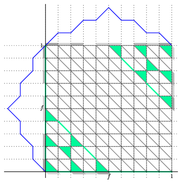
4. The Interval Lemma and its $k$-dimensional generalizations

In order to prove that a given minimal valid function $\pi$ is a facet (or an extreme function), we make use of the additivity domain $E(\pi)$ of a subadditive function $\pi\colon\mathbb{R}^{k}\to\mathbb{R}$. As discussed in the roadmap (subsection 2.3), we would like to establish that $E(\pi)\subseteq E(\pi^{\prime})$ implies $\pi=\pi^{\prime}$ for every minimal valid function $\pi^{\prime}$. An important ingredient in this step is to infer that $\pi^{\prime}$ is an affine function when restricted to projections of $E(\pi)$. For this purpose, it is convenient to separate the additivity domain into convex sets, which we then study independently. In the important case of continuous piecewise linear functions, we already know from subsection 3.5 that it suffices to study the maximal additive faces of the complex $\Delta\mathcal{P}$.

The primary object of investigation is the functional equation known as the (additive) Cauchy functional equation, which in its most general form is the study of real-valued functions $\theta$ satisfying

$$\theta({\mathchoice{\mbox{\boldmath$\displaystyle\bf u$}}{\mbox{\boldmath$\textstyle\bf u$}}{\mbox{\boldmath$\scriptstyle\bf u$}}{\mbox{\boldmath$\scriptscriptstyle\bf u$}}})+\theta({\mathchoice{\mbox{\boldmath$\displaystyle\bf v$}}{\mbox{\boldmath$\textstyle\bf v$}}{\mbox{\boldmath$\scriptstyle\bf v$}}{\mbox{\boldmath$\scriptscriptstyle\bf v$}}})=\theta({\mathchoice{\mbox{\boldmath$\displaystyle\bf u$}}{\mbox{\boldmath$\textstyle\bf u$}}{\mbox{\boldmath$\scriptstyle\bf u$}}{\mbox{\boldmath$\scriptscriptstyle\bf u$}}}+{\mathchoice{\mbox{\boldmath$\displaystyle\bf v$}}{\mbox{\boldmath$\textstyle\bf v$}}{\mbox{\boldmath$\scriptstyle\bf v$}}{\mbox{\boldmath$\scriptscriptstyle\bf v$}}}),\quad({\mathchoice{\mbox{\boldmath$\displaystyle\bf u$}}{\mbox{\boldmath$\textstyle\bf u$}}{\mbox{\boldmath$\scriptstyle\bf u$}}{\mbox{\boldmath$\scriptscriptstyle\bf u$}}},{\mathchoice{\mbox{\boldmath$\displaystyle\bf v$}}{\mbox{\boldmath$\textstyle\bf v$}}{\mbox{\boldmath$\scriptstyle\bf v$}}{\mbox{\boldmath$\scriptscriptstyle\bf v$}}})\in F$$ (15)

where $F$ is some subset of $\mathbb{R}^{k}\times\mathbb{R}^{k}$. We focus on convex sets $F$ that can be used as building blocks to cover $E(\pi)$ or other non-convex domains. The simplest convex sets $F$ of $\mathbb{R}^{k}\times\mathbb{R}^{k}$ are direct (Cartesian) products $U\times V$, where $U$ and $V$ are convex sets of $\mathbb{R}^{k}$. For $k=1$, this means we consider intervals $U\subseteq\mathbb{R}$ and $V\subseteq\mathbb{R}$ and set $F=U\times V$, i.e., we consider the functional equation $\theta(u)+\theta(v)=\theta(u+v)$ for all $u\in U$ and $v\in V$.

4.1. The classical case: Cauchy’s functional equation

Classically (see, e.g., [1, Chapter 2]), (15) is studied for the case $F=\mathbb{R}\times\mathbb{R}$. In addition to the obvious regular solutions to (15), which are the (homogeneous) linear functions $\theta(x)=cx$, there exist certain pathological solutions, which are highly discontinuous [1, Chapter 2, Theorem 3]; these were used in Propositions 2.0 and 2.0. In order to rule out these solutions, one imposes a regularity hypothesis. Various such regularity hypotheses have been proposed in the literature; for example, it is sufficient to assume that the function $\theta$ is bounded on bounded intervals [1, Chapter 2, Theorem 8].

4.2. The bounded case: Gomory–Johnson’s Interval Lemma in $\mathbb{R}^{1}$

The so-called Interval Lemma was introduced by Gomory and Johnson in [39] (the result appears implicitly in the proof of [38, Theorem 3.3]). This result concerns the Cauchy functional equation (15) on a bounded domain, i.e., the arguments $u$, $v$, and $u+v$ come from bounded intervals $U$, $V$, and their sum $U+V$, rather than the entire real line, i.e., additivity is on the set $F=U\times V$. In this case, we find that regular solutions are affine on these intervals; we lose homogeneity of the solutions. In fact, instead of equation (15), one can consider the more general equation $f(u)+g(v)=h(u+v)$, with three functions $f$, $g$, and $h$ instead of one function $\theta$.

Lemma 4.0.

(Interval Lemma) [16, LABEL:equi3:one-dim-interval_lemma] Given real numbers $u_{1}<u_{2}$ and $v_{1}<v_{2}$, let $U=[u_{1},u_{2}]$, $V=[v_{1},v_{2}]$, and $U+V=[u_{1}+v_{1},u_{2}+v_{2}]$. Let $f\colon U\rightarrow\mathbb{R}$, $g\colon V\rightarrow\mathbb{R}$, $h\colon U+V\rightarrow\mathbb{R}$ be bounded functions.
If $f(u)+g(v)=h(u+v)$ for every $(u,v)\in U\times V$, then there exists $c\in\mathbb{R}$ such that $f(u)=f(u_{1})+c(u-u_{1})$ for every $u\in U$, $g(v)=g(v_{1})+c(v-v_{1})$ for every $v\in V$, $h(w)=h(u_{1}+v_{1})+c(w-u_{1}-v_{1})$ for every $w\in U+V$. In other words, $f$, $g$ and $h$ are affine with gradient $c$ over $U$, $V$, and $U+V$ respectively.

We provide a brief justification of this result under the assumption that $f,g$ and $h$ are in $C^{2}(\mathbb{R})$ (continuous first and second derivatives). We differentiate the relation $f(u)+g(v)=h(u+v)$ with respect to $u$ (holding $v$ fixed in the interval $V$) to obtain $f^{\prime}(u)=h^{\prime}(u+v)$ for all $u\in\operatorname{int}(U)$. Since the choice of $v$ was arbitrary, this actually means $f^{\prime}(u)=h^{\prime}(u+v)$ for all $u\in\operatorname{int}(U)$ and $v\in\operatorname{int}(V)$. But then differentiating this relation with respect to $v$ we obtain $0=h^{\prime\prime}(u+v)$. This implies that $h$ is affine over $U+V$, and $f$ is affine with the same slope over $U$. Similarly, fixing $u$ in $U$ and differentiating with respect to $v$ we obtain $g^{\prime}(v)=h^{\prime}(u+v)$ for all $v\in\operatorname{int}(V)$, implying that $g$ is affine with the same slope over $V$. The result under the weaker assumption of boundedness of the functions is obtained by making a discrete version of these derivative arguments; the details are complicated and we refer the reader to [16, LABEL:equi3:one-dim-interval_lemma] for a full proof.

4.3. The full-dimensional Cartesian case: Higher-dimensional Interval Lemma

We now discuss generalization of the Interval Lemma (4.0) presented in the previous section to the $k$-dimensional setting. The first higher dimensional versions of 4.0 in the literature appear in [26, 24] for the case of $k=2$ and in [18] for general $k$, all of which apply when either $U$ or $V$ contains the origin. The result in [26] applies allows also for so-called star-shaped sets that contain the origin. We will follow the results of [16], which all for more general types of convex sets. Similar proofs of these results allow for star-shaped sets as well, but this is not presented here.

Theorem 4.1 (Higher-dimensional Interval Lemma, full-dimensional version [16, LABEL:equi3:theorem:generalized_interval_lemma_fulldim]).

Let $f,g,h\colon\allowbreak\mathbb{R}^{k}\to\mathbb{R}$ be bounded functions. Let $U$ and $V$ be convex subsets of $\mathbb{R}^{k}$ such that $f({\mathchoice{\mbox{\boldmath$\displaystyle\bf u$}}{\mbox{\boldmath$\textstyle\bf u$}}{\mbox{\boldmath$\scriptstyle\bf u$}}{\mbox{\boldmath$\scriptscriptstyle\bf u$}}})+g({\mathchoice{\mbox{\boldmath$\displaystyle\bf v$}}{\mbox{\boldmath$\textstyle\bf v$}}{\mbox{\boldmath$\scriptstyle\bf v$}}{\mbox{\boldmath$\scriptscriptstyle\bf v$}}})=h({\mathchoice{\mbox{\boldmath$\displaystyle\bf u$}}{\mbox{\boldmath$\textstyle\bf u$}}{\mbox{\boldmath$\scriptstyle\bf u$}}{\mbox{\boldmath$\scriptscriptstyle\bf u$}}}+{\mathchoice{\mbox{\boldmath$\displaystyle\bf v$}}{\mbox{\boldmath$\textstyle\bf v$}}{\mbox{\boldmath$\scriptstyle\bf v$}}{\mbox{\boldmath$\scriptscriptstyle\bf v$}}})$ for all $({\mathchoice{\mbox{\boldmath$\displaystyle\bf u$}}{\mbox{\boldmath$\textstyle\bf u$}}{\mbox{\boldmath$\scriptstyle\bf u$}}{\mbox{\boldmath$\scriptscriptstyle\bf u$}}},{\mathchoice{\mbox{\boldmath$\displaystyle\bf v$}}{\mbox{\boldmath$\textstyle\bf v$}}{\mbox{\boldmath$\scriptstyle\bf v$}}{\mbox{\boldmath$\scriptscriptstyle\bf v$}}})\in U\times V$. Assume that $\operatorname{aff}(U)=\operatorname{aff}(V)=\mathbb{R}^{k}$. Then there exists a vector ${\mathchoice{\mbox{\boldmath$\displaystyle\bf c$}}{\mbox{\boldmath$\textstyle\bf c$}}{\mbox{\boldmath$\scriptstyle\bf c$}}{\mbox{\boldmath$\scriptscriptstyle\bf c$}}}\in\mathbb{R}^{k}$ such that $f$, $g$ and $h$ are affine over $U$, $V$ and $W=U+V$, respectively, with the same gradient $\textstyle\bf c$.

4.4. The full-dimensional convex case: Cauchy’s functional equation on convex additivity domains in $\mathbb{R}^{k}$

The most direct generalization applies to full dimensional convex sets $F$.The general idea of the proof is to consider a point $({\mathchoice{\mbox{\boldmath$\displaystyle\bf x$}}{\mbox{\boldmath$\textstyle\bf x$}}{\mbox{\boldmath$\scriptstyle\bf x$}}{\mbox{\boldmath$\scriptscriptstyle\bf x$}}},{\mathchoice{\mbox{\boldmath$\displaystyle\bf y$}}{\mbox{\boldmath$\textstyle\bf y$}}{\mbox{\boldmath$\scriptstyle\bf y$}}{\mbox{\boldmath$\scriptscriptstyle\bf y$}}})$ in such a convex additivity domain $F$, and consider a finite set of smaller subsets $F_{1},\ldots,F_{k}\subseteq F$ that are Cartesian products, such that ${\mathchoice{\mbox{\boldmath$\displaystyle\bf x$}}{\mbox{\boldmath$\textstyle\bf x$}}{\mbox{\boldmath$\scriptstyle\bf x$}}{\mbox{\boldmath$\scriptscriptstyle\bf x$}}}\in F_{1}$, ${\mathchoice{\mbox{\boldmath$\displaystyle\bf y$}}{\mbox{\boldmath$\textstyle\bf y$}}{\mbox{\boldmath$\scriptstyle\bf y$}}{\mbox{\boldmath$\scriptscriptstyle\bf y$}}}\in F_{k}$ and $\operatorname{int}(F_{i})\cap\operatorname{int}(F_{i+1})\neq\emptyset$ for each $i=1,\ldots,k=1$. Applying Theorem 4.1 on each $F_{i}$, we can deduce that the functions are affine over all of $F$. This idea of “patching” together simple additivity domains to obtain affine properties over a more complicated domain was first introduced in [26, Proposition 23], and then used again in [24, Lemma 10] and [18, Lemmas 3.5, 3.6].

Theorem 4.2 (Convex additivity domain lemma, full-dimensional version [16, LABEL:equi3:lem:projection_interval_lemma_fulldim]).

Let $f,g,h\colon\mathbb{R}^{k}\to\mathbb{R}$ be bounded functions. Let $F\subseteq\mathbb{R}^{k}\times\mathbb{R}^{k}$ be a full-dimensional convex set such that $f({\mathchoice{\mbox{\boldmath$\displaystyle\bf u$}}{\mbox{\boldmath$\textstyle\bf u$}}{\mbox{\boldmath$\scriptstyle\bf u$}}{\mbox{\boldmath$\scriptscriptstyle\bf u$}}})+g({\mathchoice{\mbox{\boldmath$\displaystyle\bf v$}}{\mbox{\boldmath$\textstyle\bf v$}}{\mbox{\boldmath$\scriptstyle\bf v$}}{\mbox{\boldmath$\scriptscriptstyle\bf v$}}})=h({\mathchoice{\mbox{\boldmath$\displaystyle\bf u$}}{\mbox{\boldmath$\textstyle\bf u$}}{\mbox{\boldmath$\scriptstyle\bf u$}}{\mbox{\boldmath$\scriptscriptstyle\bf u$}}}+{\mathchoice{\mbox{\boldmath$\displaystyle\bf v$}}{\mbox{\boldmath$\textstyle\bf v$}}{\mbox{\boldmath$\scriptstyle\bf v$}}{\mbox{\boldmath$\scriptscriptstyle\bf v$}}})$ for all $({\mathchoice{\mbox{\boldmath$\displaystyle\bf u$}}{\mbox{\boldmath$\textstyle\bf u$}}{\mbox{\boldmath$\scriptstyle\bf u$}}{\mbox{\boldmath$\scriptscriptstyle\bf u$}}},{\mathchoice{\mbox{\boldmath$\displaystyle\bf v$}}{\mbox{\boldmath$\textstyle\bf v$}}{\mbox{\boldmath$\scriptstyle\bf v$}}{\mbox{\boldmath$\scriptscriptstyle\bf v$}}})\in F$. Then there exists a vector ${\mathchoice{\mbox{\boldmath$\displaystyle\bf c$}}{\mbox{\boldmath$\textstyle\bf c$}}{\mbox{\boldmath$\scriptstyle\bf c$}}{\mbox{\boldmath$\scriptscriptstyle\bf c$}}}\in\mathbb{R}^{k}$ such that $f,g$ and $h$ are affine with the same gradient $\textstyle\bf c$ over $\operatorname{int}(p_{1}(F))$, $\operatorname{int}(p_{2}(F))$ and $\operatorname{int}(p_{3}(F))$, respectively.

This theorem is obtained by applying the “patching” idea to subsets $F_{i}$ that are Cartesian products. Theorem 4.1 is applied to the individual subsets $F_{i}$ to deduce affine properties.

It is notable that we can only deduce affine linearity over the interiors of the projections in Theorem 4.2, as opposed to the conclusion of Theorem 4.1. This is best possible, as is illustrated in [16, Remark LABEL:equi3:remark:projection_interval_lemma_interiors_only]. If continuity is assumed for the functions, then one easily extends the affine-ness property to the boundary (subsection 4.6).

4.5. The lower-dimensional case: Affine properties with respect to subspaces $L$

Theorems 4.1 and 4.2 can be established in a significantly more general setting, which takes care of situations in which the set $F$ is not full-dimensional (Theorems 4.3 and 4.4). Affine properties are deduced with respect to certain subspaces, which is important for the classification of extreme functions in two or more dimensions.

We start with a result obtained in [16], in which the additivity domain is $U\times V$ for convex sets $U\subseteq\mathbb{R}^{k}$ and $V\subseteq\mathbb{R}^{k}$, which are not necessarily of the same dimension. In this general setting we cannot expect to deduce that the solutions are affine over $U$, $V$, and $U+V$.

Remark 4.2.

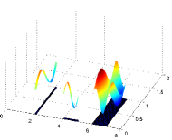
Indeed, if $U+V$ is a direct sum, i.e., for every ${\mathchoice{\mbox{\boldmath$\displaystyle\bf w$}}{\mbox{\boldmath$\textstyle\bf w$}}{\mbox{\boldmath$\scriptstyle\bf w$}}{\mbox{\boldmath$\scriptscriptstyle\bf w$}}}\in U+V$ there is a unique pair ${\mathchoice{\mbox{\boldmath$\displaystyle\bf u$}}{\mbox{\boldmath$\textstyle\bf u$}}{\mbox{\boldmath$\scriptstyle\bf u$}}{\mbox{\boldmath$\scriptscriptstyle\bf u$}}}\in U$, ${\mathchoice{\mbox{\boldmath$\displaystyle\bf v$}}{\mbox{\boldmath$\textstyle\bf v$}}{\mbox{\boldmath$\scriptstyle\bf v$}}{\mbox{\boldmath$\scriptscriptstyle\bf v$}}}\in V$ with ${\mathchoice{\mbox{\boldmath$\displaystyle\bf w$}}{\mbox{\boldmath$\textstyle\bf w$}}{\mbox{\boldmath$\scriptstyle\bf w$}}{\mbox{\boldmath$\scriptscriptstyle\bf w$}}}={\mathchoice{\mbox{\boldmath$\displaystyle\bf u$}}{\mbox{\boldmath$\textstyle\bf u$}}{\mbox{\boldmath$\scriptstyle\bf u$}}{\mbox{\boldmath$\scriptscriptstyle\bf u$}}}+{\mathchoice{\mbox{\boldmath$\displaystyle\bf v$}}{\mbox{\boldmath$\textstyle\bf v$}}{\mbox{\boldmath$\scriptstyle\bf v$}}{\mbox{\boldmath$\scriptscriptstyle\bf v$}}}$, then $f({\mathchoice{\mbox{\boldmath$\displaystyle\bf u$}}{\mbox{\boldmath$\textstyle\bf u$}}{\mbox{\boldmath$\scriptstyle\bf u$}}{\mbox{\boldmath$\scriptscriptstyle\bf u$}}})+g({\mathchoice{\mbox{\boldmath$\displaystyle\bf v$}}{\mbox{\boldmath$\textstyle\bf v$}}{\mbox{\boldmath$\scriptstyle\bf v$}}{\mbox{\boldmath$\scriptscriptstyle\bf v$}}})=h({\mathchoice{\mbox{\boldmath$\displaystyle\bf u$}}{\mbox{\boldmath$\textstyle\bf u$}}{\mbox{\boldmath$\scriptstyle\bf u$}}{\mbox{\boldmath$\scriptscriptstyle\bf u$}}}+{\mathchoice{\mbox{\boldmath$\displaystyle\bf v$}}{\mbox{\boldmath$\textstyle\bf v$}}{\mbox{\boldmath$\scriptstyle\bf v$}}{\mbox{\boldmath$\scriptscriptstyle\bf v$}}})$ merely expresses a form of separability of $h$ with respect to certain subspaces, and $f$ and $g$ can be arbitrary functions; see Figure 8 (c).

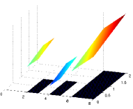
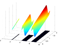
(a)                                       (b)                                       (c)

Figure 8. Cauchy’s functional equation on bounded domains. In each part (a), (b), and (c), we depict 3 domains in the plane, $U,V,U+V$, left to right, and an function that is additive over these domains. (a) Full-dimensional situation. (b) Sum of a one-dimensional and a two-dimensional set; not a direct sum. (c) Direct sum of (non-parallel) one-dimensional sets.

Definition 4.2.

Let $U\subseteq\mathbb{R}^{k}$. Given a linear subspace $L\subseteq\mathbb{R}^{k}$, we say $\pi\colon U\to\mathbb{R}$ is affine with respect to $L$ over $U$ if there exists ${\mathchoice{\mbox{\boldmath$\displaystyle\bf c$}}{\mbox{\boldmath$\textstyle\bf c$}}{\mbox{\boldmath$\scriptstyle\bf c$}}{\mbox{\boldmath$\scriptscriptstyle\bf c$}}}\in\mathbb{R}^{k}$ such that $\pi({\mathchoice{\mbox{\boldmath$\displaystyle\bf u$}}{\mbox{\boldmath$\textstyle\bf u$}}{\mbox{\boldmath$\scriptstyle\bf u$}}{\mbox{\boldmath$\scriptscriptstyle\bf u$}}}^{2})-\pi({\mathchoice{\mbox{\boldmath$\displaystyle\bf u$}}{\mbox{\boldmath$\textstyle\bf u$}}{\mbox{\boldmath$\scriptstyle\bf u$}}{\mbox{\boldmath$\scriptscriptstyle\bf u$}}}^{1})={\mathchoice{\mbox{\boldmath$\displaystyle\bf c$}}{\mbox{\boldmath$\textstyle\bf c$}}{\mbox{\boldmath$\scriptstyle\bf c$}}{\mbox{\boldmath$\scriptscriptstyle\bf c$}}}\cdot({\mathchoice{\mbox{\boldmath$\displaystyle\bf u$}}{\mbox{\boldmath$\textstyle\bf u$}}{\mbox{\boldmath$\scriptstyle\bf u$}}{\mbox{\boldmath$\scriptscriptstyle\bf u$}}}^{2}-{\mathchoice{\mbox{\boldmath$\displaystyle\bf u$}}{\mbox{\boldmath$\textstyle\bf u$}}{\mbox{\boldmath$\scriptstyle\bf u$}}{\mbox{\boldmath$\scriptscriptstyle\bf u$}}}^{1})$ for any ${\mathchoice{\mbox{\boldmath$\displaystyle\bf u$}}{\mbox{\boldmath$\textstyle\bf u$}}{\mbox{\boldmath$\scriptstyle\bf u$}}{\mbox{\boldmath$\scriptscriptstyle\bf u$}}}^{1},{\mathchoice{\mbox{\boldmath$\displaystyle\bf u$}}{\mbox{\boldmath$\textstyle\bf u$}}{\mbox{\boldmath$\scriptstyle\bf u$}}{\mbox{\boldmath$\scriptscriptstyle\bf u$}}}^{2}\in U$ such that ${\mathchoice{\mbox{\boldmath$\displaystyle\bf u$}}{\mbox{\boldmath$\textstyle\bf u$}}{\mbox{\boldmath$\scriptstyle\bf u$}}{\mbox{\boldmath$\scriptscriptstyle\bf u$}}}^{2}-{\mathchoice{\mbox{\boldmath$\displaystyle\bf u$}}{\mbox{\boldmath$\textstyle\bf u$}}{\mbox{\boldmath$\scriptstyle\bf u$}}{\mbox{\boldmath$\scriptscriptstyle\bf u$}}}^{1}\in L$.

Theorem 4.3 (Higher-dimensional Interval Lemma; [16, LABEL:equi3:lem:generalized_interval_lemma]).

Let $f,g,h\colon\mathbb{R}^{k}\to\mathbb{R}$ be bounded functions. Let $U$ and $V$ be convex subsets of $\mathbb{R}^{k}$ such that $f({\mathchoice{\mbox{\boldmath$\displaystyle\bf u$}}{\mbox{\boldmath$\textstyle\bf u$}}{\mbox{\boldmath$\scriptstyle\bf u$}}{\mbox{\boldmath$\scriptscriptstyle\bf u$}}})+g({\mathchoice{\mbox{\boldmath$\displaystyle\bf v$}}{\mbox{\boldmath$\textstyle\bf v$}}{\mbox{\boldmath$\scriptstyle\bf v$}}{\mbox{\boldmath$\scriptscriptstyle\bf v$}}})=h({\mathchoice{\mbox{\boldmath$\displaystyle\bf u$}}{\mbox{\boldmath$\textstyle\bf u$}}{\mbox{\boldmath$\scriptstyle\bf u$}}{\mbox{\boldmath$\scriptscriptstyle\bf u$}}}+{\mathchoice{\mbox{\boldmath$\displaystyle\bf v$}}{\mbox{\boldmath$\textstyle\bf v$}}{\mbox{\boldmath$\scriptstyle\bf v$}}{\mbox{\boldmath$\scriptscriptstyle\bf v$}}})$ for all $({\mathchoice{\mbox{\boldmath$\displaystyle\bf u$}}{\mbox{\boldmath$\textstyle\bf u$}}{\mbox{\boldmath$\scriptstyle\bf u$}}{\mbox{\boldmath$\scriptscriptstyle\bf u$}}},{\mathchoice{\mbox{\boldmath$\displaystyle\bf v$}}{\mbox{\boldmath$\textstyle\bf v$}}{\mbox{\boldmath$\scriptstyle\bf v$}}{\mbox{\boldmath$\scriptscriptstyle\bf v$}}})\in F=U\times V$. Let $L$ be a linear subspace of $\mathbb{R}^{k}$ such that $(L+U)\times(L+V)=(L\times L)+F\subseteq\operatorname{aff}(F)=\operatorname{aff}(U)\times\operatorname{aff}(V)$. Then there exists a vector ${\mathchoice{\mbox{\boldmath$\displaystyle\bf c$}}{\mbox{\boldmath$\textstyle\bf c$}}{\mbox{\boldmath$\scriptstyle\bf c$}}{\mbox{\boldmath$\scriptscriptstyle\bf c$}}}\in\mathbb{R}^{k}$ such that $f$, $g$ and $h$ are affine with respect to $L$ over $p_{1}(F)=U$, $p_{2}(F)=V$ and $p_{3}(F)=U+V$ respectively, with gradient $\textstyle\bf c$.

Theorem 4.1 follows when $L=\mathbb{R}^{k}$.

Definition 4.3.

For a linear space $L\subseteq\mathbb{R}^{k}$ and a set $U\subseteq\mathbb{R}^{k}$ such that for some ${\mathchoice{\mbox{\boldmath$\displaystyle\bf u$}}{\mbox{\boldmath$\textstyle\bf u$}}{\mbox{\boldmath$\scriptstyle\bf u$}}{\mbox{\boldmath$\scriptscriptstyle\bf u$}}}\in\mathbb{R}^{k}$ we have $\operatorname{aff}(U)\subseteq L+{\mathchoice{\mbox{\boldmath$\displaystyle\bf u$}}{\mbox{\boldmath$\textstyle\bf u$}}{\mbox{\boldmath$\scriptstyle\bf u$}}{\mbox{\boldmath$\scriptscriptstyle\bf u$}}}$, we will denote by $\operatorname{int}_{L}(U)$ the interior of $U$ in the relative topology of $L+{\mathchoice{\mbox{\boldmath$\displaystyle\bf u$}}{\mbox{\boldmath$\textstyle\bf u$}}{\mbox{\boldmath$\scriptstyle\bf u$}}{\mbox{\boldmath$\scriptscriptstyle\bf u$}}}$.

Note that $\operatorname{int}_{L}(U)$ is well defined because either $\operatorname{aff}(U)=L+{\mathchoice{\mbox{\boldmath$\displaystyle\bf u$}}{\mbox{\boldmath$\textstyle\bf u$}}{\mbox{\boldmath$\scriptstyle\bf u$}}{\mbox{\boldmath$\scriptscriptstyle\bf u$}}}$, or $\operatorname{int}_{L}(U)=\emptyset$. We now state our most general theorem relating to equation (15) on a convex domain.

Theorem 4.4 (Convex additivity domain lemma; [16, LABEL:equi3:lem:projection_interval_lemma]).

Let $f,g,h\colon\mathbb{R}^{k}\to\mathbb{R}$ be bounded functions. Let $F\subseteq\mathbb{R}^{k}\times\mathbb{R}^{k}$ be a convex set such that $f({\mathchoice{\mbox{\boldmath$\displaystyle\bf u$}}{\mbox{\boldmath$\textstyle\bf u$}}{\mbox{\boldmath$\scriptstyle\bf u$}}{\mbox{\boldmath$\scriptscriptstyle\bf u$}}})+g({\mathchoice{\mbox{\boldmath$\displaystyle\bf v$}}{\mbox{\boldmath$\textstyle\bf v$}}{\mbox{\boldmath$\scriptstyle\bf v$}}{\mbox{\boldmath$\scriptscriptstyle\bf v$}}})=h({\mathchoice{\mbox{\boldmath$\displaystyle\bf u$}}{\mbox{\boldmath$\textstyle\bf u$}}{\mbox{\boldmath$\scriptstyle\bf u$}}{\mbox{\boldmath$\scriptscriptstyle\bf u$}}}+{\mathchoice{\mbox{\boldmath$\displaystyle\bf v$}}{\mbox{\boldmath$\textstyle\bf v$}}{\mbox{\boldmath$\scriptstyle\bf v$}}{\mbox{\boldmath$\scriptscriptstyle\bf v$}}})$ for all $({\mathchoice{\mbox{\boldmath$\displaystyle\bf u$}}{\mbox{\boldmath$\textstyle\bf u$}}{\mbox{\boldmath$\scriptstyle\bf u$}}{\mbox{\boldmath$\scriptscriptstyle\bf u$}}},{\mathchoice{\mbox{\boldmath$\displaystyle\bf v$}}{\mbox{\boldmath$\textstyle\bf v$}}{\mbox{\boldmath$\scriptstyle\bf v$}}{\mbox{\boldmath$\scriptscriptstyle\bf v$}}})\in F$. Let $L$ be a linear subspace of $\mathbb{R}^{k}$ such that $(L\times L)+F\subseteq\operatorname{aff}(F)$. Let $({\mathchoice{\mbox{\boldmath$\displaystyle\bf u$}}{\mbox{\boldmath$\textstyle\bf u$}}{\mbox{\boldmath$\scriptstyle\bf u$}}{\mbox{\boldmath$\scriptscriptstyle\bf u$}}}^{0},{\mathchoice{\mbox{\boldmath$\displaystyle\bf v$}}{\mbox{\boldmath$\textstyle\bf v$}}{\mbox{\boldmath$\scriptstyle\bf v$}}{\mbox{\boldmath$\scriptscriptstyle\bf v$}}}^{0})\in\operatorname{rel\,int}(F)$. Then there exists a vector ${\mathchoice{\mbox{\boldmath$\displaystyle\bf c$}}{\mbox{\boldmath$\textstyle\bf c$}}{\mbox{\boldmath$\scriptstyle\bf c$}}{\mbox{\boldmath$\scriptscriptstyle\bf c$}}}\in\mathbb{R}^{k}$ such that $f,g$ and $h$ are affine with gradient $\textstyle\bf c$ over $\operatorname{int}_{L}(({\mathchoice{\mbox{\boldmath$\displaystyle\bf u$}}{\mbox{\boldmath$\textstyle\bf u$}}{\mbox{\boldmath$\scriptstyle\bf u$}}{\mbox{\boldmath$\scriptscriptstyle\bf u$}}}^{0}+L)\cap p_{1}(F))$, $\operatorname{int}_{L}(({\mathchoice{\mbox{\boldmath$\displaystyle\bf v$}}{\mbox{\boldmath$\textstyle\bf v$}}{\mbox{\boldmath$\scriptstyle\bf v$}}{\mbox{\boldmath$\scriptscriptstyle\bf v$}}}^{0}+L)\cap p_{2}(F))$ and $\operatorname{int}_{L}(({\mathchoice{\mbox{\boldmath$\displaystyle\bf u$}}{\mbox{\boldmath$\textstyle\bf u$}}{\mbox{\boldmath$\scriptstyle\bf u$}}{\mbox{\boldmath$\scriptscriptstyle\bf u$}}}^{0}+{\mathchoice{\mbox{\boldmath$\displaystyle\bf v$}}{\mbox{\boldmath$\textstyle\bf v$}}{\mbox{\boldmath$\scriptstyle\bf v$}}{\mbox{\boldmath$\scriptscriptstyle\bf v$}}}^{0}+L)\cap p_{3}(F))$, respectively.

Theorem 4.2 follows when $L=\mathbb{R}^{k}$.

4.6. Continuity at the boundary

The one-dimensional Interval Lemma, Lemma 4.0, includes affine properties on the boundaries. Using this, it is easy to prove that a similar Interval Lemma holds on all non-degenerate intervals $U,V\subseteq\mathbb{R}$ that are any of open, half-open, or closed. Only in special cases in higher dimensions is it possible to extend affine properties in Theorem 4.4 to the boundary; in general this is not possible (see [16, Remark LABEL:equi3:remark:projection_interval_lemma_interiors_only]).

Of course, if we use the stronger regularity assumption that $f$, $g$, and $h$ are continuous functions (rather than merely bounded functions), then the affine properties extend to the boundary as well.

Corollary 4.4 (Convex additivity domain lemma for continuous functions; [16, LABEL:equi3:lem:projection_interval_lemma-corollary])).

Let $f,g,h\colon\mathbb{R}^{k}\to\mathbb{R}$ be continuous functions. Let $F\subseteq\mathbb{R}^{k}\times\mathbb{R}^{k}$ be a convex set such that $f({\mathchoice{\mbox{\boldmath$\displaystyle\bf u$}}{\mbox{\boldmath$\textstyle\bf u$}}{\mbox{\boldmath$\scriptstyle\bf u$}}{\mbox{\boldmath$\scriptscriptstyle\bf u$}}})+g({\mathchoice{\mbox{\boldmath$\displaystyle\bf v$}}{\mbox{\boldmath$\textstyle\bf v$}}{\mbox{\boldmath$\scriptstyle\bf v$}}{\mbox{\boldmath$\scriptscriptstyle\bf v$}}})=h({\mathchoice{\mbox{\boldmath$\displaystyle\bf u$}}{\mbox{\boldmath$\textstyle\bf u$}}{\mbox{\boldmath$\scriptstyle\bf u$}}{\mbox{\boldmath$\scriptscriptstyle\bf u$}}}+{\mathchoice{\mbox{\boldmath$\displaystyle\bf v$}}{\mbox{\boldmath$\textstyle\bf v$}}{\mbox{\boldmath$\scriptstyle\bf v$}}{\mbox{\boldmath$\scriptscriptstyle\bf v$}}})$ for all $({\mathchoice{\mbox{\boldmath$\displaystyle\bf u$}}{\mbox{\boldmath$\textstyle\bf u$}}{\mbox{\boldmath$\scriptstyle\bf u$}}{\mbox{\boldmath$\scriptscriptstyle\bf u$}}},{\mathchoice{\mbox{\boldmath$\displaystyle\bf v$}}{\mbox{\boldmath$\textstyle\bf v$}}{\mbox{\boldmath$\scriptstyle\bf v$}}{\mbox{\boldmath$\scriptscriptstyle\bf v$}}})\in F$. Let $L$ be a linear subspace of $\mathbb{R}^{k}$ such that $L\times L+F\subseteq\operatorname{aff}(F)$. Let $({\mathchoice{\mbox{\boldmath$\displaystyle\bf u$}}{\mbox{\boldmath$\textstyle\bf u$}}{\mbox{\boldmath$\scriptstyle\bf u$}}{\mbox{\boldmath$\scriptscriptstyle\bf u$}}}^{0},{\mathchoice{\mbox{\boldmath$\displaystyle\bf v$}}{\mbox{\boldmath$\textstyle\bf v$}}{\mbox{\boldmath$\scriptstyle\bf v$}}{\mbox{\boldmath$\scriptscriptstyle\bf v$}}}^{0})\in\operatorname{rel\,int}(F)$. Then there exists a vector ${\mathchoice{\mbox{\boldmath$\displaystyle\bf c$}}{\mbox{\boldmath$\textstyle\bf c$}}{\mbox{\boldmath$\scriptstyle\bf c$}}{\mbox{\boldmath$\scriptscriptstyle\bf c$}}}\in\mathbb{R}^{k}$ such that $f,g$ and $h$ are affine with gradient $\textstyle\bf c$ over $({\mathchoice{\mbox{\boldmath$\displaystyle\bf u$}}{\mbox{\boldmath$\textstyle\bf u$}}{\mbox{\boldmath$\scriptstyle\bf u$}}{\mbox{\boldmath$\scriptscriptstyle\bf u$}}}^{0}+L)\cap p_{1}(F)$, $({\mathchoice{\mbox{\boldmath$\displaystyle\bf v$}}{\mbox{\boldmath$\textstyle\bf v$}}{\mbox{\boldmath$\scriptstyle\bf v$}}{\mbox{\boldmath$\scriptscriptstyle\bf v$}}}^{0}+L)\cap p_{2}(F)$ and $({\mathchoice{\mbox{\boldmath$\displaystyle\bf u$}}{\mbox{\boldmath$\textstyle\bf u$}}{\mbox{\boldmath$\scriptstyle\bf u$}}{\mbox{\boldmath$\scriptscriptstyle\bf u$}}}^{0}+{\mathchoice{\mbox{\boldmath$\displaystyle\bf v$}}{\mbox{\boldmath$\textstyle\bf v$}}{\mbox{\boldmath$\scriptstyle\bf v$}}{\mbox{\boldmath$\scriptscriptstyle\bf v$}}}^{0}+L)\cap p_{3}(F)$, respectively.

5. Sufficient conditions for extremality in the $k$-row infinite group problem

5.1. The $(k+1)$-Slope Theorem

We have already mentioned the classic Gomory–Johnson 2-Slope Theorem (Theorem 2.3), which states that for $k=1$, if a continuous piecewise linear minimal function has only 2 slopes, then it is extreme. An analogous 3-Slope Theorem for $k=2$ was proved by Cornuéjols and Molinaro [24]. We present here the $(k+1)$-Slope Theorem for the case of general $k$ by Basu, Hildebrand, Köppe and Molinaro [18], along with the main ingredients of its proof.

Theorem 5.1 ([18, Theorem 1.7]).

Let $\pi\colon\mathbb{R}^{k}\to\mathbb{R}$ be a minimal valid function that is continuous piecewise linear and genuinely $k$-dimensional with at most $k+1$ slopes, i.e., at most $k+1$ different values for the gradient of $\pi$ where it exists. Then $\pi$ is extreme and has exactly $k+1$ slopes.

The proof will follow the basic roadmap of subsection 2.3 and use 2.1; we give an outline here, before diving into the details. For the rest of this section, $\pi$ is a continuous piecewise linear minimal function that is genuinely $k$-dimensional with at most $k+1$ slopes. Let $\mathcal{P}$ be the associated polyhedral complex.

1. Subadditivity and the property of being genuinely $k$-dimensional is used to first establish that $\pi$ has exactly $k+1$ gradient values ${\mathchoice{\mbox{\boldmath$\displaystyle\bf\bar{g}$}}{\mbox{\boldmath$\textstyle\bf\bar{g}$}}{\mbox{\boldmath$\scriptstyle\bf\bar{g}$}}{\mbox{\boldmath$\scriptscriptstyle\bf\bar{g}$}}}^{1},\ldots,{\mathchoice{\mbox{\boldmath$\displaystyle\bf\bar{g}$}}{\mbox{\boldmath$\textstyle\bf\bar{g}$}}{\mbox{\boldmath$\scriptstyle\bf\bar{g}$}}{\mbox{\boldmath$\scriptscriptstyle\bf\bar{g}$}}}^{k+1}\in\mathbb{R}^{k}$. This is a relatively easy step, and we refer to the reader to [18, Lemma 2.11] for the details.

2. Consider any minimal valid functions $\pi^{1},\pi^{2}$ such that $\pi=\frac{\pi^{1}+\pi^{2}}{2}$.

3. (Compatibility step) For each $i=1,\ldots,k+1$, define $\mathcal{P}_{i}\subseteq\mathcal{P}$ to be the polyhedral complex formed by all the cells (and their faces) of $\mathcal{P}$ where the gradient of $\pi$ is ${\mathchoice{\mbox{\boldmath$\displaystyle\bf\bar{g}$}}{\mbox{\boldmath$\textstyle\bf\bar{g}$}}{\mbox{\boldmath$\scriptstyle\bf\bar{g}$}}{\mbox{\boldmath$\scriptscriptstyle\bf\bar{g}$}}}^{i}$. Show that there exist ${\mathchoice{\mbox{\boldmath$\displaystyle\bf\tilde{g}$}}{\mbox{\boldmath$\textstyle\bf\tilde{g}$}}{\mbox{\boldmath$\scriptstyle\bf\tilde{g}$}}{\mbox{\boldmath$\scriptscriptstyle\bf\tilde{g}$}}}^{1},\ldots,{\mathchoice{\mbox{\boldmath$\displaystyle\bf\tilde{g}$}}{\mbox{\boldmath$\textstyle\bf\tilde{g}$}}{\mbox{\boldmath$\scriptstyle\bf\tilde{g}$}}{\mbox{\boldmath$\scriptscriptstyle\bf\tilde{g}$}}}^{k+1}$ such that $\pi^{1}$ is affine over every cell in $\mathcal{P}_{i}$ with gradient ${\mathchoice{\mbox{\boldmath$\displaystyle\bf\tilde{g}$}}{\mbox{\boldmath$\textstyle\bf\tilde{g}$}}{\mbox{\boldmath$\scriptstyle\bf\tilde{g}$}}{\mbox{\boldmath$\scriptscriptstyle\bf\tilde{g}$}}}^{i}$.

4. (Gradient matching step) We then highlight certain structures of genuinely $k$-dimensional functions with $k+1$ slopes that lead to a system of $k(k+1)$ equations that are satisfied by the coefficients of ${\mathchoice{\mbox{\boldmath$\displaystyle\bf\bar{g}$}}{\mbox{\boldmath$\textstyle\bf\bar{g}$}}{\mbox{\boldmath$\scriptstyle\bf\bar{g}$}}{\mbox{\boldmath$\scriptscriptstyle\bf\bar{g}$}}}^{1},\ldots,{\mathchoice{\mbox{\boldmath$\displaystyle\bf\bar{g}$}}{\mbox{\boldmath$\textstyle\bf\bar{g}$}}{\mbox{\boldmath$\scriptstyle\bf\bar{g}$}}{\mbox{\boldmath$\scriptscriptstyle\bf\bar{g}$}}}^{k+1}$ and ${\mathchoice{\mbox{\boldmath$\displaystyle\bf\tilde{g}$}}{\mbox{\boldmath$\textstyle\bf\tilde{g}$}}{\mbox{\boldmath$\scriptstyle\bf\tilde{g}$}}{\mbox{\boldmath$\scriptscriptstyle\bf\tilde{g}$}}}^{1},\ldots,{\mathchoice{\mbox{\boldmath$\displaystyle\bf\tilde{g}$}}{\mbox{\boldmath$\textstyle\bf\tilde{g}$}}{\mbox{\boldmath$\scriptstyle\bf\tilde{g}$}}{\mbox{\boldmath$\scriptscriptstyle\bf\tilde{g}$}}}^{k+1}$. Then, it is established that this system of equations has a unique solution, and thus, ${\mathchoice{\mbox{\boldmath$\displaystyle\bf\bar{g}$}}{\mbox{\boldmath$\textstyle\bf\bar{g}$}}{\mbox{\boldmath$\scriptstyle\bf\bar{g}$}}{\mbox{\boldmath$\scriptscriptstyle\bf\bar{g}$}}}^{i}={\mathchoice{\mbox{\boldmath$\displaystyle\bf\tilde{g}$}}{\mbox{\boldmath$\textstyle\bf\tilde{g}$}}{\mbox{\boldmath$\scriptstyle\bf\tilde{g}$}}{\mbox{\boldmath$\scriptscriptstyle\bf\tilde{g}$}}}^{i}$ for every $i=1,\ldots,k+1$.

5. For every ${\mathchoice{\mbox{\boldmath$\displaystyle\bf r$}}{\mbox{\boldmath$\textstyle\bf r$}}{\mbox{\boldmath$\scriptstyle\bf r$}}{\mbox{\boldmath$\scriptscriptstyle\bf r$}}}\in\mathbb{R}^{k}$ there exist $\mu_{1},\mu_{2},\ldots,\mu_{k+1}$ such that $\mu_{i}$ is the fraction of the segment $[{\mathchoice{\mbox{\boldmath$\displaystyle\bf 0$}}{\mbox{\boldmath$\textstyle\bf 0$}}{\mbox{\boldmath$\scriptstyle\bf 0$}}{\mbox{\boldmath$\scriptscriptstyle\bf 0$}}},{\mathchoice{\mbox{\boldmath$\displaystyle\bf r$}}{\mbox{\boldmath$\textstyle\bf r$}}{\mbox{\boldmath$\scriptstyle\bf r$}}{\mbox{\boldmath$\scriptscriptstyle\bf r$}}}]$ that lies in $\mathcal{P}_{i}$. Thus,

   $$\pi({\mathchoice{\mbox{\boldmath$\displaystyle\bf r$}}{\mbox{\boldmath$\textstyle\bf r$}}{\mbox{\boldmath$\scriptstyle\bf r$}}{\mbox{\boldmath$\scriptscriptstyle\bf r$}}})=\pi({\mathchoice{\mbox{\boldmath$\displaystyle\bf 0$}}{\mbox{\boldmath$\textstyle\bf 0$}}{\mbox{\boldmath$\scriptstyle\bf 0$}}{\mbox{\boldmath$\scriptscriptstyle\bf 0$}}})+\sum_{i=1}^{k+1}\mu_{i}({\mathchoice{\mbox{\boldmath$\displaystyle\bf\bar{g}$}}{\mbox{\boldmath$\textstyle\bf\bar{g}$}}{\mbox{\boldmath$\scriptstyle\bf\bar{g}$}}{\mbox{\boldmath$\scriptscriptstyle\bf\bar{g}$}}}^{i}\cdot{\mathchoice{\mbox{\boldmath$\displaystyle\bf r$}}{\mbox{\boldmath$\textstyle\bf r$}}{\mbox{\boldmath$\scriptstyle\bf r$}}{\mbox{\boldmath$\scriptscriptstyle\bf r$}}})=\pi^{1}({\mathchoice{\mbox{\boldmath$\displaystyle\bf 0$}}{\mbox{\boldmath$\textstyle\bf 0$}}{\mbox{\boldmath$\scriptstyle\bf 0$}}{\mbox{\boldmath$\scriptscriptstyle\bf 0$}}})+\sum_{i=1}^{k+1}\mu_{i}({\mathchoice{\mbox{\boldmath$\displaystyle\bf\tilde{g}$}}{\mbox{\boldmath$\textstyle\bf\tilde{g}$}}{\mbox{\boldmath$\scriptstyle\bf\tilde{g}$}}{\mbox{\boldmath$\scriptscriptstyle\bf\tilde{g}$}}}^{i}\cdot{\mathchoice{\mbox{\boldmath$\displaystyle\bf r$}}{\mbox{\boldmath$\textstyle\bf r$}}{\mbox{\boldmath$\scriptstyle\bf r$}}{\mbox{\boldmath$\scriptscriptstyle\bf r$}}})=\pi^{1}({\mathchoice{\mbox{\boldmath$\displaystyle\bf r$}}{\mbox{\boldmath$\textstyle\bf r$}}{\mbox{\boldmath$\scriptstyle\bf r$}}{\mbox{\boldmath$\scriptscriptstyle\bf r$}}}).$$

   This proves that $\pi=\pi^{1}$ and thus, $\pi=\pi^{1}=\pi^{2}$, concluding the proof of Theorem 5.1.

Compatibility Step.

The following observation is crucial:

Lemma 5.1.

Let $U,V\subseteq\mathbb{R}^{k}$ be full-dimensional convex sets such that ${\mathchoice{\mbox{\boldmath$\displaystyle\bf 0$}}{\mbox{\boldmath$\textstyle\bf 0$}}{\mbox{\boldmath$\scriptstyle\bf 0$}}{\mbox{\boldmath$\scriptscriptstyle\bf 0$}}}\in U$. Let $F=F(U,V,V)$. Then ${\mathchoice{\mbox{\boldmath$\displaystyle\bf 0$}}{\mbox{\boldmath$\textstyle\bf 0$}}{\mbox{\boldmath$\scriptstyle\bf 0$}}{\mbox{\boldmath$\scriptscriptstyle\bf 0$}}}\in p_{1}(F)$, $V=p_{2}(F)=p_{3}(F)$ and $p_{1}(F)$ is full-dimensional. Furthermore, if $\pi\colon\mathbb{R}^{k}\to\mathbb{R}$ is such that $\pi({\mathchoice{\mbox{\boldmath$\displaystyle\bf 0$}}{\mbox{\boldmath$\textstyle\bf 0$}}{\mbox{\boldmath$\scriptstyle\bf 0$}}{\mbox{\boldmath$\scriptscriptstyle\bf 0$}}})=0$ and is affine on $U,V$ with the same slope, then $F\subseteq E(\pi)$.

Proof.

By definition, $p_{1}(F)\subseteq U,p_{2}(F),p_{3}(F)\subseteq V$. Since ${\mathchoice{\mbox{\boldmath$\displaystyle\bf 0$}}{\mbox{\boldmath$\textstyle\bf 0$}}{\mbox{\boldmath$\scriptstyle\bf 0$}}{\mbox{\boldmath$\scriptscriptstyle\bf 0$}}}\in U$ and $\{{\mathchoice{\mbox{\boldmath$\displaystyle\bf 0$}}{\mbox{\boldmath$\textstyle\bf 0$}}{\mbox{\boldmath$\scriptstyle\bf 0$}}{\mbox{\boldmath$\scriptscriptstyle\bf 0$}}}\}+V=V$, we see that $p_{2}(F),p_{3}(F)=V$ and ${\mathchoice{\mbox{\boldmath$\displaystyle\bf 0$}}{\mbox{\boldmath$\textstyle\bf 0$}}{\mbox{\boldmath$\scriptstyle\bf 0$}}{\mbox{\boldmath$\scriptscriptstyle\bf 0$}}}\in p_{1}(F)$. Now, let ${\mathchoice{\mbox{\boldmath$\displaystyle\bf v$}}{\mbox{\boldmath$\textstyle\bf v$}}{\mbox{\boldmath$\scriptstyle\bf v$}}{\mbox{\boldmath$\scriptscriptstyle\bf v$}}}\in\operatorname{int}(V)$. Therefore there exists a ball $B({\mathchoice{\mbox{\boldmath$\displaystyle\bf v$}}{\mbox{\boldmath$\textstyle\bf v$}}{\mbox{\boldmath$\scriptstyle\bf v$}}{\mbox{\boldmath$\scriptscriptstyle\bf v$}}},\epsilon)\subseteq V$. Since $U$ is full-dimensional, there exist $k$-linearly independent vectors ${\mathchoice{\mbox{\boldmath$\displaystyle\bf u$}}{\mbox{\boldmath$\textstyle\bf u$}}{\mbox{\boldmath$\scriptstyle\bf u$}}{\mbox{\boldmath$\scriptscriptstyle\bf u$}}}^{1},\dots,{\mathchoice{\mbox{\boldmath$\displaystyle\bf u$}}{\mbox{\boldmath$\textstyle\bf u$}}{\mbox{\boldmath$\scriptstyle\bf u$}}{\mbox{\boldmath$\scriptscriptstyle\bf u$}}}^{k}\in U$ with $\|{\mathchoice{\mbox{\boldmath$\displaystyle\bf u$}}{\mbox{\boldmath$\textstyle\bf u$}}{\mbox{\boldmath$\scriptstyle\bf u$}}{\mbox{\boldmath$\scriptscriptstyle\bf u$}}}^{i}\|\leq\epsilon$. But then ${\mathchoice{\mbox{\boldmath$\displaystyle\bf u$}}{\mbox{\boldmath$\textstyle\bf u$}}{\mbox{\boldmath$\scriptstyle\bf u$}}{\mbox{\boldmath$\scriptscriptstyle\bf u$}}}^{i}+{\mathchoice{\mbox{\boldmath$\displaystyle\bf v$}}{\mbox{\boldmath$\textstyle\bf v$}}{\mbox{\boldmath$\scriptstyle\bf v$}}{\mbox{\boldmath$\scriptscriptstyle\bf v$}}}\in V$. Therefore, ${\mathchoice{\mbox{\boldmath$\displaystyle\bf u$}}{\mbox{\boldmath$\textstyle\bf u$}}{\mbox{\boldmath$\scriptstyle\bf u$}}{\mbox{\boldmath$\scriptscriptstyle\bf u$}}}^{i}\in p_{1}(F)$. Finally, since $F$ is convex and the projection of convex sets is convex, we have that $p_{1}(F)$ is full-dimensional.

For the second part of the lemma, observe that there exist ${\mathchoice{\mbox{\boldmath$\displaystyle\bf g$}}{\mbox{\boldmath$\textstyle\bf g$}}{\mbox{\boldmath$\scriptstyle\bf g$}}{\mbox{\boldmath$\scriptscriptstyle\bf g$}}}\in\mathbb{R}^{k}$ and $\delta\in\mathbb{R}$ be such that $\pi({\mathchoice{\mbox{\boldmath$\displaystyle\bf u$}}{\mbox{\boldmath$\textstyle\bf u$}}{\mbox{\boldmath$\scriptstyle\bf u$}}{\mbox{\boldmath$\scriptscriptstyle\bf u$}}})={\mathchoice{\mbox{\boldmath$\displaystyle\bf g$}}{\mbox{\boldmath$\textstyle\bf g$}}{\mbox{\boldmath$\scriptstyle\bf g$}}{\mbox{\boldmath$\scriptscriptstyle\bf g$}}}\cdot{\mathchoice{\mbox{\boldmath$\displaystyle\bf u$}}{\mbox{\boldmath$\textstyle\bf u$}}{\mbox{\boldmath$\scriptstyle\bf u$}}{\mbox{\boldmath$\scriptscriptstyle\bf u$}}}$ (follows since ${\mathchoice{\mbox{\boldmath$\displaystyle\bf 0$}}{\mbox{\boldmath$\textstyle\bf 0$}}{\mbox{\boldmath$\scriptstyle\bf 0$}}{\mbox{\boldmath$\scriptscriptstyle\bf 0$}}}\in U$ and $\pi({\mathchoice{\mbox{\boldmath$\displaystyle\bf 0$}}{\mbox{\boldmath$\textstyle\bf 0$}}{\mbox{\boldmath$\scriptstyle\bf 0$}}{\mbox{\boldmath$\scriptscriptstyle\bf 0$}}})=0$) for all ${\mathchoice{\mbox{\boldmath$\displaystyle\bf u$}}{\mbox{\boldmath$\textstyle\bf u$}}{\mbox{\boldmath$\scriptstyle\bf u$}}{\mbox{\boldmath$\scriptscriptstyle\bf u$}}}\in U$ and $\pi({\mathchoice{\mbox{\boldmath$\displaystyle\bf v$}}{\mbox{\boldmath$\textstyle\bf v$}}{\mbox{\boldmath$\scriptstyle\bf v$}}{\mbox{\boldmath$\scriptscriptstyle\bf v$}}})={\mathchoice{\mbox{\boldmath$\displaystyle\bf g$}}{\mbox{\boldmath$\textstyle\bf g$}}{\mbox{\boldmath$\scriptstyle\bf g$}}{\mbox{\boldmath$\scriptscriptstyle\bf g$}}}\cdot{\mathchoice{\mbox{\boldmath$\displaystyle\bf v$}}{\mbox{\boldmath$\textstyle\bf v$}}{\mbox{\boldmath$\scriptstyle\bf v$}}{\mbox{\boldmath$\scriptscriptstyle\bf v$}}}+\delta$ for all ${\mathchoice{\mbox{\boldmath$\displaystyle\bf v$}}{\mbox{\boldmath$\textstyle\bf v$}}{\mbox{\boldmath$\scriptstyle\bf v$}}{\mbox{\boldmath$\scriptscriptstyle\bf v$}}}\in V$. Then for any ${\mathchoice{\mbox{\boldmath$\displaystyle\bf u$}}{\mbox{\boldmath$\textstyle\bf u$}}{\mbox{\boldmath$\scriptstyle\bf u$}}{\mbox{\boldmath$\scriptscriptstyle\bf u$}}}\in U,{\mathchoice{\mbox{\boldmath$\displaystyle\bf v$}}{\mbox{\boldmath$\textstyle\bf v$}}{\mbox{\boldmath$\scriptstyle\bf v$}}{\mbox{\boldmath$\scriptscriptstyle\bf v$}}}\in V$ with ${\mathchoice{\mbox{\boldmath$\displaystyle\bf u$}}{\mbox{\boldmath$\textstyle\bf u$}}{\mbox{\boldmath$\scriptstyle\bf u$}}{\mbox{\boldmath$\scriptscriptstyle\bf u$}}}+{\mathchoice{\mbox{\boldmath$\displaystyle\bf v$}}{\mbox{\boldmath$\textstyle\bf v$}}{\mbox{\boldmath$\scriptstyle\bf v$}}{\mbox{\boldmath$\scriptscriptstyle\bf v$}}}\in V$, we have $\pi({\mathchoice{\mbox{\boldmath$\displaystyle\bf u$}}{\mbox{\boldmath$\textstyle\bf u$}}{\mbox{\boldmath$\scriptstyle\bf u$}}{\mbox{\boldmath$\scriptscriptstyle\bf u$}}})+\pi({\mathchoice{\mbox{\boldmath$\displaystyle\bf v$}}{\mbox{\boldmath$\textstyle\bf v$}}{\mbox{\boldmath$\scriptstyle\bf v$}}{\mbox{\boldmath$\scriptscriptstyle\bf v$}}})-\pi({\mathchoice{\mbox{\boldmath$\displaystyle\bf u$}}{\mbox{\boldmath$\textstyle\bf u$}}{\mbox{\boldmath$\scriptstyle\bf u$}}{\mbox{\boldmath$\scriptscriptstyle\bf u$}}}+{\mathchoice{\mbox{\boldmath$\displaystyle\bf v$}}{\mbox{\boldmath$\textstyle\bf v$}}{\mbox{\boldmath$\scriptstyle\bf v$}}{\mbox{\boldmath$\scriptscriptstyle\bf v$}}})=({\mathchoice{\mbox{\boldmath$\displaystyle\bf g$}}{\mbox{\boldmath$\textstyle\bf g$}}{\mbox{\boldmath$\scriptstyle\bf g$}}{\mbox{\boldmath$\scriptscriptstyle\bf g$}}}\cdot{\mathchoice{\mbox{\boldmath$\displaystyle\bf u$}}{\mbox{\boldmath$\textstyle\bf u$}}{\mbox{\boldmath$\scriptstyle\bf u$}}{\mbox{\boldmath$\scriptscriptstyle\bf u$}}})+({\mathchoice{\mbox{\boldmath$\displaystyle\bf g$}}{\mbox{\boldmath$\textstyle\bf g$}}{\mbox{\boldmath$\scriptstyle\bf g$}}{\mbox{\boldmath$\scriptscriptstyle\bf g$}}}\cdot{\mathchoice{\mbox{\boldmath$\displaystyle\bf v$}}{\mbox{\boldmath$\textstyle\bf v$}}{\mbox{\boldmath$\scriptstyle\bf v$}}{\mbox{\boldmath$\scriptscriptstyle\bf v$}}}+\delta)-({\mathchoice{\mbox{\boldmath$\displaystyle\bf g$}}{\mbox{\boldmath$\textstyle\bf g$}}{\mbox{\boldmath$\scriptstyle\bf g$}}{\mbox{\boldmath$\scriptscriptstyle\bf g$}}}\cdot({\mathchoice{\mbox{\boldmath$\displaystyle\bf u$}}{\mbox{\boldmath$\textstyle\bf u$}}{\mbox{\boldmath$\scriptstyle\bf u$}}{\mbox{\boldmath$\scriptscriptstyle\bf u$}}}+{\mathchoice{\mbox{\boldmath$\displaystyle\bf v$}}{\mbox{\boldmath$\textstyle\bf v$}}{\mbox{\boldmath$\scriptstyle\bf v$}}{\mbox{\boldmath$\scriptscriptstyle\bf v$}}})+\delta)=0$. ∎

The analysis of step (1) also shows that for every $i=1,\ldots,k+1$, there exist $C_{i}\in\mathcal{P}_{i}$ such that ${\mathchoice{\mbox{\boldmath$\displaystyle\bf 0$}}{\mbox{\boldmath$\textstyle\bf 0$}}{\mbox{\boldmath$\scriptstyle\bf 0$}}{\mbox{\boldmath$\scriptscriptstyle\bf 0$}}}\in C_{i}$ (in other words, for every gradient value, there is a cell containing the origin with that gradient). Fix an arbitrary $i\in\{1,\ldots,k+1\}$ and consider any cell $P\in\mathcal{P}_{i}$. By 5.1 with $U=C_{i}$ and $V=P$, we obtain that $F=F(C_{i},V,V)\subseteq E(\pi)$. By 2.1 (ii), $F\subseteq E(\pi^{1})$ and by 2.1 (iii), $\pi^{1}$ is continuous. By Theorem 4.2 and continuity of $\pi^{1}$, we obtain that $\pi^{1}$ is affine on $C_{i}$ and $P$ with the same gradient. Since the choice of $P$ was arbitrary, this establishes that for every cell $P\in P_{i}$, $\pi^{1}$ is affine with the same gradient; this is precisely the desired ${\mathchoice{\mbox{\boldmath$\displaystyle\bf\tilde{g}$}}{\mbox{\boldmath$\textstyle\bf\tilde{g}$}}{\mbox{\boldmath$\scriptstyle\bf\tilde{g}$}}{\mbox{\boldmath$\scriptscriptstyle\bf\tilde{g}$}}}^{i}$.

Gradient matching step.

The system for step (4) has two sets of constraints, the first of which follows from the condition that $\pi({\mathchoice{\mbox{\boldmath$\displaystyle\bf f$}}{\mbox{\boldmath$\textstyle\bf f$}}{\mbox{\boldmath$\scriptstyle\bf f$}}{\mbox{\boldmath$\scriptscriptstyle\bf f$}}}+{\mathchoice{\mbox{\boldmath$\displaystyle\bf w$}}{\mbox{\boldmath$\textstyle\bf w$}}{\mbox{\boldmath$\scriptstyle\bf w$}}{\mbox{\boldmath$\scriptscriptstyle\bf w$}}})=1$ for every ${\mathchoice{\mbox{\boldmath$\displaystyle\bf w$}}{\mbox{\boldmath$\textstyle\bf w$}}{\mbox{\boldmath$\scriptstyle\bf w$}}{\mbox{\boldmath$\scriptscriptstyle\bf w$}}}\in\mathbb{Z}^{k}$. The second set of constraints is more involved. Consider two adjacent cells $P,P^{\prime}\in\mathcal{P}$ that contain a segment $[{\mathchoice{\mbox{\boldmath$\displaystyle\bf x$}}{\mbox{\boldmath$\textstyle\bf x$}}{\mbox{\boldmath$\scriptstyle\bf x$}}{\mbox{\boldmath$\scriptscriptstyle\bf x$}}},{\mathchoice{\mbox{\boldmath$\displaystyle\bf y$}}{\mbox{\boldmath$\textstyle\bf y$}}{\mbox{\boldmath$\scriptstyle\bf y$}}{\mbox{\boldmath$\scriptscriptstyle\bf y$}}}]\subseteq\mathbb{R}^{k}$ in their intersection. Along the line segment $[{\mathchoice{\mbox{\boldmath$\displaystyle\bf x$}}{\mbox{\boldmath$\textstyle\bf x$}}{\mbox{\boldmath$\scriptstyle\bf x$}}{\mbox{\boldmath$\scriptscriptstyle\bf x$}}},{\mathchoice{\mbox{\boldmath$\displaystyle\bf y$}}{\mbox{\boldmath$\textstyle\bf y$}}{\mbox{\boldmath$\scriptstyle\bf y$}}{\mbox{\boldmath$\scriptscriptstyle\bf y$}}}]$, the gradients of $P$ and $P^{\prime}$ projected onto the line spanned by the vector ${\mathchoice{\mbox{\boldmath$\displaystyle\bf y$}}{\mbox{\boldmath$\textstyle\bf y$}}{\mbox{\boldmath$\scriptstyle\bf y$}}{\mbox{\boldmath$\scriptscriptstyle\bf y$}}}-{\mathchoice{\mbox{\boldmath$\displaystyle\bf x$}}{\mbox{\boldmath$\textstyle\bf x$}}{\mbox{\boldmath$\scriptstyle\bf x$}}{\mbox{\boldmath$\scriptscriptstyle\bf x$}}}$ must agree; the second set of constraints captures this observation. We will identify a set of vectors ${\mathchoice{\mbox{\boldmath$\displaystyle\bf r$}}{\mbox{\boldmath$\textstyle\bf r$}}{\mbox{\boldmath$\scriptstyle\bf r$}}{\mbox{\boldmath$\scriptscriptstyle\bf r$}}}^{1},\ldots,{\mathchoice{\mbox{\boldmath$\displaystyle\bf r$}}{\mbox{\boldmath$\textstyle\bf r$}}{\mbox{\boldmath$\scriptstyle\bf r$}}{\mbox{\boldmath$\scriptscriptstyle\bf r$}}}^{k+1}$ such that every subset of $k$ vectors is linearly independent and such that each vector ${\mathchoice{\mbox{\boldmath$\displaystyle\bf r$}}{\mbox{\boldmath$\textstyle\bf r$}}{\mbox{\boldmath$\scriptstyle\bf r$}}{\mbox{\boldmath$\scriptscriptstyle\bf r$}}}^{i}$ is contained in $k$ cells of $\mathcal{P}$ with different gradients. We then use the segment $[{\mathchoice{\mbox{\boldmath$\displaystyle\bf 0$}}{\mbox{\boldmath$\textstyle\bf 0$}}{\mbox{\boldmath$\scriptstyle\bf 0$}}{\mbox{\boldmath$\scriptscriptstyle\bf 0$}}},{\mathchoice{\mbox{\boldmath$\displaystyle\bf r$}}{\mbox{\boldmath$\textstyle\bf r$}}{\mbox{\boldmath$\scriptstyle\bf r$}}{\mbox{\boldmath$\scriptscriptstyle\bf r$}}}^{i}]$ to obtain linear equations involving the gradients of $\pi$ and $\pi^{\prime}$. The fact that every subset of $k$ vectors is linearly independent will be crucial in ensuring the uniqueness of the system of equations.

Lemma 5.1 ([18, Lemma 3.10]).

There exist vectors ${\mathchoice{\mbox{\boldmath$\displaystyle\bf r$}}{\mbox{\boldmath$\textstyle\bf r$}}{\mbox{\boldmath$\scriptstyle\bf r$}}{\mbox{\boldmath$\scriptscriptstyle\bf r$}}}^{1},{\mathchoice{\mbox{\boldmath$\displaystyle\bf r$}}{\mbox{\boldmath$\textstyle\bf r$}}{\mbox{\boldmath$\scriptstyle\bf r$}}{\mbox{\boldmath$\scriptscriptstyle\bf r$}}}^{2},\ldots,{\mathchoice{\mbox{\boldmath$\displaystyle\bf r$}}{\mbox{\boldmath$\textstyle\bf r$}}{\mbox{\boldmath$\scriptstyle\bf r$}}{\mbox{\boldmath$\scriptscriptstyle\bf r$}}}^{k+1}\in\mathbb{R}^{k}$ with the following properties:

1. For every $i,j,\ell\in\{1,\ldots,k+1\}$ with $j,\ell$ different from $i$, the equations ${\mathchoice{\mbox{\boldmath$\displaystyle\bf r$}}{\mbox{\boldmath$\textstyle\bf r$}}{\mbox{\boldmath$\scriptstyle\bf r$}}{\mbox{\boldmath$\scriptscriptstyle\bf r$}}}^{i}\cdot{\mathchoice{\mbox{\boldmath$\displaystyle\bf\bar{g}$}}{\mbox{\boldmath$\textstyle\bf\bar{g}$}}{\mbox{\boldmath$\scriptstyle\bf\bar{g}$}}{\mbox{\boldmath$\scriptscriptstyle\bf\bar{g}$}}}^{j}={\mathchoice{\mbox{\boldmath$\displaystyle\bf r$}}{\mbox{\boldmath$\textstyle\bf r$}}{\mbox{\boldmath$\scriptstyle\bf r$}}{\mbox{\boldmath$\scriptscriptstyle\bf r$}}}^{i}\cdot{\mathchoice{\mbox{\boldmath$\displaystyle\bf\bar{g}$}}{\mbox{\boldmath$\textstyle\bf\bar{g}$}}{\mbox{\boldmath$\scriptstyle\bf\bar{g}$}}{\mbox{\boldmath$\scriptscriptstyle\bf\bar{g}$}}}^{\ell}$ and ${\mathchoice{\mbox{\boldmath$\displaystyle\bf r$}}{\mbox{\boldmath$\textstyle\bf r$}}{\mbox{\boldmath$\scriptstyle\bf r$}}{\mbox{\boldmath$\scriptscriptstyle\bf r$}}}^{i}\cdot{\mathchoice{\mbox{\boldmath$\displaystyle\bf\tilde{g}$}}{\mbox{\boldmath$\textstyle\bf\tilde{g}$}}{\mbox{\boldmath$\scriptstyle\bf\tilde{g}$}}{\mbox{\boldmath$\scriptscriptstyle\bf\tilde{g}$}}}^{j}={\mathchoice{\mbox{\boldmath$\displaystyle\bf r$}}{\mbox{\boldmath$\textstyle\bf r$}}{\mbox{\boldmath$\scriptstyle\bf r$}}{\mbox{\boldmath$\scriptscriptstyle\bf r$}}}^{i}\cdot{\mathchoice{\mbox{\boldmath$\displaystyle\bf\tilde{g}$}}{\mbox{\boldmath$\textstyle\bf\tilde{g}$}}{\mbox{\boldmath$\scriptstyle\bf\tilde{g}$}}{\mbox{\boldmath$\scriptscriptstyle\bf\tilde{g}$}}}^{\ell}$ hold.

2. Every $k$-subset of $\{{\mathchoice{\mbox{\boldmath$\displaystyle\bf r$}}{\mbox{\boldmath$\textstyle\bf r$}}{\mbox{\boldmath$\scriptstyle\bf r$}}{\mbox{\boldmath$\scriptscriptstyle\bf r$}}}^{1},\ldots,{\mathchoice{\mbox{\boldmath$\displaystyle\bf r$}}{\mbox{\boldmath$\textstyle\bf r$}}{\mbox{\boldmath$\scriptstyle\bf r$}}{\mbox{\boldmath$\scriptscriptstyle\bf r$}}}^{k+1}\}$ is linearly independent.

Figure 9. The geometry of the proof of 5.1. Each cone $C_{i}$ (shaded in dark colors) is the intersection of the halfspaces $H_{j}$ (defined by the gradients $\bar{\mathchoice{\mbox{\boldmath$\displaystyle\bf g$}}{\mbox{\boldmath$\textstyle\bf g$}}{\mbox{\boldmath$\scriptstyle\bf g$}}{\mbox{\boldmath$\scriptscriptstyle\bf g$}}}^{j}$) for $j\neq i$. Near the origin (within the ball $B({\mathchoice{\mbox{\boldmath$\displaystyle\bf 0$}}{\mbox{\boldmath$\textstyle\bf 0$}}{\mbox{\boldmath$\scriptstyle\bf 0$}}{\mbox{\boldmath$\scriptscriptstyle\bf 0$}}},\varepsilon)$), each point of $C_{i}$ lies in the set $F_{i}$ of points where the function $\pi$ has gradient $\bar{\mathchoice{\mbox{\boldmath$\displaystyle\bf g$}}{\mbox{\boldmath$\textstyle\bf g$}}{\mbox{\boldmath$\scriptstyle\bf g$}}{\mbox{\boldmath$\scriptscriptstyle\bf g$}}}^{i}$ (shaded in light colors). Picking points $\mathchoice{\mbox{\boldmath$\displaystyle\bf v$}}{\mbox{\boldmath$\textstyle\bf v$}}{\mbox{\boldmath$\scriptstyle\bf v$}}{\mbox{\boldmath$\scriptscriptstyle\bf v$}}_{i}$ near the origin in the interior of $C_{i}$, we construct a simplex $\Delta$ with $\textstyle\bf 0$ in its interior. By applying the KKM Lemma to each of its facets $\Delta_{i}$, we show the existence of the vectors ${\mathchoice{\mbox{\boldmath$\displaystyle\bf r$}}{\mbox{\boldmath$\textstyle\bf r$}}{\mbox{\boldmath$\scriptstyle\bf r$}}{\mbox{\boldmath$\scriptscriptstyle\bf r$}}}^{i}$ with the desired properties.

The proof of 5.1 uses a nontrivial result known as the Knaster–Kuratowski–Mazurkiewicz Lemma (KKM Lemma) from fixed point theory, which exposes a nice structure in the gradient pattern of $\pi$. The KKM lemma states that if a $d$-dimensional simplex is covered by $d+1$ closed sets satisfying certain combinatorial conditions, then there is a point in the intersection of all $d+1$ sets. This lemma is applied to the facets of a certain simplex $S$ containing the origin, where the closed sets form $S\cap\mathcal{P}_{i}$. The fixed points on the $k+1$ facets of this simplex give the vectors ${\mathchoice{\mbox{\boldmath$\displaystyle\bf r$}}{\mbox{\boldmath$\textstyle\bf r$}}{\mbox{\boldmath$\scriptstyle\bf r$}}{\mbox{\boldmath$\scriptscriptstyle\bf r$}}}^{1},\ldots,{\mathchoice{\mbox{\boldmath$\displaystyle\bf r$}}{\mbox{\boldmath$\textstyle\bf r$}}{\mbox{\boldmath$\scriptstyle\bf r$}}{\mbox{\boldmath$\scriptscriptstyle\bf r$}}}^{k+1}$ from 5.1. The bulk of the technicality lies in showing that the hypothesis of the KKM lemma are satisfied by the gradient structure of $\pi$. A few more details are offered in Figure 9.

We finally present the system of linear equations that we consider.

Corollary 5.1 ([18, Corollary 3.13]).

Consider any $k+1$ affinely independent vectors ${\mathchoice{\mbox{\boldmath$\displaystyle\bf a$}}{\mbox{\boldmath$\textstyle\bf a$}}{\mbox{\boldmath$\scriptstyle\bf a$}}{\mbox{\boldmath$\scriptscriptstyle\bf a$}}}^{1},{\mathchoice{\mbox{\boldmath$\displaystyle\bf a$}}{\mbox{\boldmath$\textstyle\bf a$}}{\mbox{\boldmath$\scriptstyle\bf a$}}{\mbox{\boldmath$\scriptscriptstyle\bf a$}}}^{2},\ldots,{\mathchoice{\mbox{\boldmath$\displaystyle\bf a$}}{\mbox{\boldmath$\textstyle\bf a$}}{\mbox{\boldmath$\scriptstyle\bf a$}}{\mbox{\boldmath$\scriptscriptstyle\bf a$}}}^{k+1}\in\mathbb{Z}^{k}+{\mathchoice{\mbox{\boldmath$\displaystyle\bf f$}}{\mbox{\boldmath$\textstyle\bf f$}}{\mbox{\boldmath$\scriptstyle\bf f$}}{\mbox{\boldmath$\scriptscriptstyle\bf f$}}}$. Also, let ${\mathchoice{\mbox{\boldmath$\displaystyle\bf r$}}{\mbox{\boldmath$\textstyle\bf r$}}{\mbox{\boldmath$\scriptstyle\bf r$}}{\mbox{\boldmath$\scriptscriptstyle\bf r$}}}^{1},{\mathchoice{\mbox{\boldmath$\displaystyle\bf r$}}{\mbox{\boldmath$\textstyle\bf r$}}{\mbox{\boldmath$\scriptstyle\bf r$}}{\mbox{\boldmath$\scriptscriptstyle\bf r$}}}^{2},\ldots,{\mathchoice{\mbox{\boldmath$\displaystyle\bf r$}}{\mbox{\boldmath$\textstyle\bf r$}}{\mbox{\boldmath$\scriptstyle\bf r$}}{\mbox{\boldmath$\scriptscriptstyle\bf r$}}}^{k+1}$ be the vectors given by 5.1. Then there exist $\mu_{ij}\in\mathbb{R}_{+}$, $i,j\in\{1,\ldots,k+1\}$ with $\sum_{j=1}^{k+1}\mu_{ij}=1$ for all $i\in\{1,\ldots,k+1\}$ such that both ${\mathchoice{\mbox{\boldmath$\displaystyle\bf\tilde{g}$}}{\mbox{\boldmath$\textstyle\bf\tilde{g}$}}{\mbox{\boldmath$\scriptstyle\bf\tilde{g}$}}{\mbox{\boldmath$\scriptscriptstyle\bf\tilde{g}$}}}^{1},\ldots,{\mathchoice{\mbox{\boldmath$\displaystyle\bf\tilde{g}$}}{\mbox{\boldmath$\textstyle\bf\tilde{g}$}}{\mbox{\boldmath$\scriptstyle\bf\tilde{g}$}}{\mbox{\boldmath$\scriptscriptstyle\bf\tilde{g}$}}}^{k+1}$ and ${\mathchoice{\mbox{\boldmath$\displaystyle\bf\bar{g}$}}{\mbox{\boldmath$\textstyle\bf\bar{g}$}}{\mbox{\boldmath$\scriptstyle\bf\bar{g}$}}{\mbox{\boldmath$\scriptscriptstyle\bf\bar{g}$}}}^{1},\ldots,{\mathchoice{\mbox{\boldmath$\displaystyle\bf\bar{g}$}}{\mbox{\boldmath$\textstyle\bf\bar{g}$}}{\mbox{\boldmath$\scriptstyle\bf\bar{g}$}}{\mbox{\boldmath$\scriptscriptstyle\bf\bar{g}$}}}^{k+1}$ are solutions to the linear system

$$\textstyle\sum_{j=1}^{k+1}(\mu_{ij}{\mathchoice{\mbox{\boldmath$\displaystyle\bf a$}}{\mbox{\boldmath$\textstyle\bf a$}}{\mbox{\boldmath$\scriptstyle\bf a$}}{\mbox{\boldmath$\scriptscriptstyle\bf a$}}}^{i})\cdot{\mathchoice{\mbox{\boldmath$\displaystyle\bf g$}}{\mbox{\boldmath$\textstyle\bf g$}}{\mbox{\boldmath$\scriptstyle\bf g$}}{\mbox{\boldmath$\scriptscriptstyle\bf g$}}}^{j} =1 \text{for all }i\in\{1,\ldots,k+1\},$$ (16)

$${\mathchoice{\mbox{\boldmath$\displaystyle\bf r$}}{\mbox{\boldmath$\textstyle\bf r$}}{\mbox{\boldmath$\scriptstyle\bf r$}}{\mbox{\boldmath$\scriptscriptstyle\bf r$}}}^{i}\cdot{\mathchoice{\mbox{\boldmath$\displaystyle\bf g$}}{\mbox{\boldmath$\textstyle\bf g$}}{\mbox{\boldmath$\scriptstyle\bf g$}}{\mbox{\boldmath$\scriptscriptstyle\bf g$}}}^{j}-{\mathchoice{\mbox{\boldmath$\displaystyle\bf r$}}{\mbox{\boldmath$\textstyle\bf r$}}{\mbox{\boldmath$\scriptstyle\bf r$}}{\mbox{\boldmath$\scriptscriptstyle\bf r$}}}^{i}\cdot{\mathchoice{\mbox{\boldmath$\displaystyle\bf g$}}{\mbox{\boldmath$\textstyle\bf g$}}{\mbox{\boldmath$\scriptstyle\bf g$}}{\mbox{\boldmath$\scriptscriptstyle\bf g$}}}^{\ell} =0 \text{for all }i,j,\ell\in\{1,\ldots,k+1\}\textrm{ such that }i\neq j,\ell,$$

with variables ${\mathchoice{\mbox{\boldmath$\displaystyle\bf g$}}{\mbox{\boldmath$\textstyle\bf g$}}{\mbox{\boldmath$\scriptstyle\bf g$}}{\mbox{\boldmath$\scriptscriptstyle\bf g$}}}^{1},\ldots,{\mathchoice{\mbox{\boldmath$\displaystyle\bf g$}}{\mbox{\boldmath$\textstyle\bf g$}}{\mbox{\boldmath$\scriptstyle\bf g$}}{\mbox{\boldmath$\scriptscriptstyle\bf g$}}}^{k+1}\in\mathbb{R}^{k}$.

We remark that we can always find vectors ${\mathchoice{\mbox{\boldmath$\displaystyle\bf a$}}{\mbox{\boldmath$\textstyle\bf a$}}{\mbox{\boldmath$\scriptstyle\bf a$}}{\mbox{\boldmath$\scriptscriptstyle\bf a$}}}^{1},{\mathchoice{\mbox{\boldmath$\displaystyle\bf a$}}{\mbox{\boldmath$\textstyle\bf a$}}{\mbox{\boldmath$\scriptstyle\bf a$}}{\mbox{\boldmath$\scriptscriptstyle\bf a$}}}^{2},\ldots,{\mathchoice{\mbox{\boldmath$\displaystyle\bf a$}}{\mbox{\boldmath$\textstyle\bf a$}}{\mbox{\boldmath$\scriptstyle\bf a$}}{\mbox{\boldmath$\scriptscriptstyle\bf a$}}}^{k+1}\in\mathbb{Z}^{k}+{\mathchoice{\mbox{\boldmath$\displaystyle\bf f$}}{\mbox{\boldmath$\textstyle\bf f$}}{\mbox{\boldmath$\scriptstyle\bf f$}}{\mbox{\boldmath$\scriptscriptstyle\bf f$}}}$ such that the set ${\mathchoice{\mbox{\boldmath$\displaystyle\bf a$}}{\mbox{\boldmath$\textstyle\bf a$}}{\mbox{\boldmath$\scriptstyle\bf a$}}{\mbox{\boldmath$\scriptscriptstyle\bf a$}}}^{1},\ldots,{\mathchoice{\mbox{\boldmath$\displaystyle\bf a$}}{\mbox{\boldmath$\textstyle\bf a$}}{\mbox{\boldmath$\scriptstyle\bf a$}}{\mbox{\boldmath$\scriptscriptstyle\bf a$}}}^{k+1}$ is affinely independent, so the system above indeed exists. Property (ii) in 5.1 and the fact that ${\mathchoice{\mbox{\boldmath$\displaystyle\bf a$}}{\mbox{\boldmath$\textstyle\bf a$}}{\mbox{\boldmath$\scriptstyle\bf a$}}{\mbox{\boldmath$\scriptscriptstyle\bf a$}}}^{1},\ldots,{\mathchoice{\mbox{\boldmath$\displaystyle\bf a$}}{\mbox{\boldmath$\textstyle\bf a$}}{\mbox{\boldmath$\scriptstyle\bf a$}}{\mbox{\boldmath$\scriptscriptstyle\bf a$}}}^{k+1}$ are affinely independent can be used to show that (16) has either no solutions or a unique solution. Since ${\mathchoice{\mbox{\boldmath$\displaystyle\bf\bar{g}$}}{\mbox{\boldmath$\textstyle\bf\bar{g}$}}{\mbox{\boldmath$\scriptstyle\bf\bar{g}$}}{\mbox{\boldmath$\scriptscriptstyle\bf\bar{g}$}}}^{1},\ldots,{\mathchoice{\mbox{\boldmath$\displaystyle\bf\bar{g}$}}{\mbox{\boldmath$\textstyle\bf\bar{g}$}}{\mbox{\boldmath$\scriptstyle\bf\bar{g}$}}{\mbox{\boldmath$\scriptscriptstyle\bf\bar{g}$}}}^{k+1}$ is a solution, the conclusion is that the system has a unique solution and so ${\mathchoice{\mbox{\boldmath$\displaystyle\bf\tilde{g}$}}{\mbox{\boldmath$\textstyle\bf\tilde{g}$}}{\mbox{\boldmath$\scriptstyle\bf\tilde{g}$}}{\mbox{\boldmath$\scriptscriptstyle\bf\tilde{g}$}}}^{j}={\mathchoice{\mbox{\boldmath$\displaystyle\bf\bar{g}$}}{\mbox{\boldmath$\textstyle\bf\bar{g}$}}{\mbox{\boldmath$\scriptstyle\bf\bar{g}$}}{\mbox{\boldmath$\scriptscriptstyle\bf\bar{g}$}}}^{j}$ for each $j=1,\ldots,k+1$.

Remark 5.1.

Along almost identical lines, one can show that a $(k+1)$-slope function $\pi$ is a facet – this is done in [18]. The only difference is that the continuity of $\pi^{1}$ in the proof above was obtained easily via Lemma 2.1 (iii). For the facetness proof, this continuity argument is slightly more involved.

5.2. Construction of extreme functions with the sequential-merge procedure

Dey and Richard [27] gave the first examples of facets in higher dimensions by combining facets from lower dimensions. We outline these concepts here. For a more detailed discussion, we refer the reader to [27] and also the survey [48].

Let $\varphi\colon\mathbb{R}\to\mathbb{R}$ be valid for $R_{f_{k+1}}(\mathbb{R},\mathbb{Z})$ and $\pi\colon\mathbb{R}^{k}\to\mathbb{R}$ valid for $R_{\mathchoice{\mbox{\boldmath$\displaystyle\bf f$}}{\mbox{\boldmath$\textstyle\bf f$}}{\mbox{\boldmath$\scriptstyle\bf f$}}{\mbox{\boldmath$\scriptscriptstyle\bf f$}}}(\mathbb{R}^{k},\mathbb{Z}^{k})$. The sequential merge of $\varphi$ and $\pi$ is the function $\varphi\mathbin{\lozenge}\pi\colon\mathbb{R}^{k}\times\mathbb{R}\to\mathbb{R}$ given by

$$(\varphi\mathbin{\lozenge}\pi)({\mathchoice{\mbox{\boldmath$\displaystyle\bf x$}}{\mbox{\boldmath$\textstyle\bf x$}}{\mbox{\boldmath$\scriptstyle\bf x$}}{\mbox{\boldmath$\scriptscriptstyle\bf x$}}},x_{k+1})=\frac{\pi({\mathchoice{\mbox{\boldmath$\displaystyle\bf x$}}{\mbox{\boldmath$\textstyle\bf x$}}{\mbox{\boldmath$\scriptstyle\bf x$}}{\mbox{\boldmath$\scriptscriptstyle\bf x$}}})\sum_{i=1}^{k}f_{i}+f_{k+1}\varphi\Big{(}\sum_{i=1}^{k+1}x_{i}-\pi({\mathchoice{\mbox{\boldmath$\displaystyle\bf x$}}{\mbox{\boldmath$\textstyle\bf x$}}{\mbox{\boldmath$\scriptstyle\bf x$}}{\mbox{\boldmath$\scriptscriptstyle\bf x$}}})\sum_{i=1}^{k}f_{i}\Big{)}}{\sum_{i=1}^{k+1}f_{i}}.$$

Here we assume, without loss of generality, that $f_{k+1}\in(0,1)$, ${\mathchoice{\mbox{\boldmath$\displaystyle\bf f$}}{\mbox{\boldmath$\textstyle\bf f$}}{\mbox{\boldmath$\scriptstyle\bf f$}}{\mbox{\boldmath$\scriptscriptstyle\bf f$}}}\in[0,1)^{k}\setminus\{{\mathchoice{\mbox{\boldmath$\displaystyle\bf 0$}}{\mbox{\boldmath$\textstyle\bf 0$}}{\mbox{\boldmath$\scriptstyle\bf 0$}}{\mbox{\boldmath$\scriptscriptstyle\bf 0$}}}\}$. The lifting space representation of a function $\pi\colon\mathbb{R}^{k}\to\mathbb{R}$ is given by $[\pi]_{\mathchoice{\mbox{\boldmath$\displaystyle\bf f$}}{\mbox{\boldmath$\textstyle\bf f$}}{\mbox{\boldmath$\scriptstyle\bf f$}}{\mbox{\boldmath$\scriptscriptstyle\bf f$}}}({\mathchoice{\mbox{\boldmath$\displaystyle\bf x$}}{\mbox{\boldmath$\textstyle\bf x$}}{\mbox{\boldmath$\scriptstyle\bf x$}}{\mbox{\boldmath$\scriptscriptstyle\bf x$}}})=\sum_{i=1}^{k}x_{i}-\pi({\mathchoice{\mbox{\boldmath$\displaystyle\bf x$}}{\mbox{\boldmath$\textstyle\bf x$}}{\mbox{\boldmath$\scriptstyle\bf x$}}{\mbox{\boldmath$\scriptscriptstyle\bf x$}}})\sum_{i=1}^{k}f_{i}$.

Dey and Richard showed that $(\varphi\mathbin{\lozenge}\pi)({\mathchoice{\mbox{\boldmath$\displaystyle\bf x$}}{\mbox{\boldmath$\textstyle\bf x$}}{\mbox{\boldmath$\scriptstyle\bf x$}}{\mbox{\boldmath$\scriptscriptstyle\bf x$}}},x_{k+1})$ is a facet for $R_{({\mathchoice{\mbox{\boldmath$\displaystyle\bf f$}}{\mbox{\boldmath$\textstyle\bf f$}}{\mbox{\boldmath$\scriptstyle\bf f$}}{\mbox{\boldmath$\scriptscriptstyle\bf f$}}},f_{k+1})}(\mathbb{R}^{k+1},\mathbb{Z}^{k+1})$ provided that $\varphi$ and $\pi$ are facets, their lifting representations are non-decreasing, and the perturbation spaces $\bar{\Pi}^{E(\varphi)}(\mathbb{R},\mathbb{Z})$ and $\bar{\Pi}^{E(\pi)}(\mathbb{R}^{k},\mathbb{Z}^{k})$ both contain only trivial solutions [27, Theorem 5]. They also show how to extend these sequential merge facets to facets of the mixed-integer problem [27, Proposition 15]. This produces a simple method to construct facets in higher dimensions from facets in lower dimensions.

Some sequential merge functions can be projected as well. Let $\xi\colon\mathbb{R}\to\mathbb{R}$ be the gmic function and let $\pi\colon\mathbb{R}\to\mathbb{R}$ be a valid function for $R_{f}(\mathbb{R},\mathbb{Z})$. For any $n\in\mathbb{Z}_{+}$ such that $0<f<1/n$, we define the projected sequential merge function $\pi\mathbin{\lozenge_{n}^{1}}\xi\colon\mathbb{R}\to\mathbb{R}$ as $(\pi\mathbin{\lozenge_{n}^{1}}\xi)(x)=(\pi\mathbin{\lozenge}\xi)(nx,x)$. Provided that $\pi$ is a facet of $R_{f}(\mathbb{R},\mathbb{Z})$ and $[\pi]_{f}$ is non-decreasing and $\bar{\Pi}^{E(\pi)}(\mathbb{R},\mathbb{Z})$ has only the trivial solution, we have that $\pi\mathbin{\lozenge_{n}^{1}}\xi$ is a facet for $R_{nf}(\mathbb{R},\mathbb{Z})$. See Table 5 for an example of a projected sequential merge inequality, dr_projected_sequential_merge_3_slope. Also dg_2_step_mir from Table 1 can be seen as the projected sequential merge function $\xi\mathbin{\lozenge_{n}^{1}}\xi$. We can state this idea in the following more general way. Consider $(\pi_{1}\mathbin{\lozenge}(\pi_{2}\mathbin{\lozenge}\dots(\pi_{k-1}\mathbin{\lozenge}\pi_{k})\ldots))$, where $\pi_{i}$ is a facet for $R_{f}(\mathbb{R},\mathbb{Z})$ and $[\pi_{i}]_{f}$ is non-decreasing, and $\bar{\Pi}^{E(\pi^{i})}(\mathbb{R},\mathbb{Z})$ has only the trivial solution for $i=1,\dots,k$. Let $n\in\mathbb{Z}_{+}$ such that $0<f_{k}<\tfrac{1}{n}$. Then $(\pi_{1}\mathbin{\lozenge}(\pi_{2}\mathbin{\lozenge}\dots\mathbin{\lozenge}(\pi_{k-1}\mathbin{\lozenge}(\pi_{k}\mathbin{\lozenge_{n}^{1}}\xi))\ldots))$ is a facet for $R_{{\mathchoice{\mbox{\boldmath$\displaystyle\bf f$}}{\mbox{\boldmath$\textstyle\bf f$}}{\mbox{\boldmath$\scriptstyle\bf f$}}{\mbox{\boldmath$\scriptscriptstyle\bf f$}}}^{\prime}}(\mathbb{R}^{k},\mathbb{Z}^{k})$ where ${\mathchoice{\mbox{\boldmath$\displaystyle\bf f$}}{\mbox{\boldmath$\textstyle\bf f$}}{\mbox{\boldmath$\scriptstyle\bf f$}}{\mbox{\boldmath$\scriptscriptstyle\bf f$}}}^{\prime}=(f_{1},\dots,f_{k-1},nf_{k})$ [27, Theorem 6].

6. Sequences of minimal valid and extreme functions

6.1. Minimality of limits of minimal valid functions

The most basic topology on the space $\mathbb{R}^{G}$ of real-valued functions on $G$ is the product topology, or the topology of pointwise convergence. We first note that the properties in the characterization of minimal valid functions (Theorem 2.1) are preserved under pointwise convergence.

Proposition 6.0 ([28, Proposition 4]).

Let $\pi_{i}\in\mathbb{R}^{G}$, $i\in\mathbb{N}$ be a sequence of minimal valid functions that converge pointwise to $\pi\in\mathbb{R}^{G}$. Then $\pi$ is a minimal valid function.

Proof.

Since each $\pi_{i}$ is nonnegative, $\pi$ is nonnegative. We simply verify the conditions in Theorem 2.1 for $\pi$.

1. For any $\mathchoice{\mbox{\boldmath$\displaystyle\bf w$}}{\mbox{\boldmath$\textstyle\bf w$}}{\mbox{\boldmath$\scriptstyle\bf w$}}{\mbox{\boldmath$\scriptscriptstyle\bf w$}}\in S$, $\pi(\mathchoice{\mbox{\boldmath$\displaystyle\bf w$}}{\mbox{\boldmath$\textstyle\bf w$}}{\mbox{\boldmath$\scriptstyle\bf w$}}{\mbox{\boldmath$\scriptscriptstyle\bf w$}})=\lim_{i\to\infty}\pi_{i}(\mathchoice{\mbox{\boldmath$\displaystyle\bf w$}}{\mbox{\boldmath$\textstyle\bf w$}}{\mbox{\boldmath$\scriptstyle\bf w$}}{\mbox{\boldmath$\scriptscriptstyle\bf w$}})=\lim_{i\to\infty}0=0$.

2. For any $\mathchoice{\mbox{\boldmath$\displaystyle\bf x$}}{\mbox{\boldmath$\textstyle\bf x$}}{\mbox{\boldmath$\scriptstyle\bf x$}}{\mbox{\boldmath$\scriptscriptstyle\bf x$}},\mathchoice{\mbox{\boldmath$\displaystyle\bf y$}}{\mbox{\boldmath$\textstyle\bf y$}}{\mbox{\boldmath$\scriptstyle\bf y$}}{\mbox{\boldmath$\scriptscriptstyle\bf y$}}\in G$, $\pi(\mathchoice{\mbox{\boldmath$\displaystyle\bf x$}}{\mbox{\boldmath$\textstyle\bf x$}}{\mbox{\boldmath$\scriptstyle\bf x$}}{\mbox{\boldmath$\scriptscriptstyle\bf x$}}+\mathchoice{\mbox{\boldmath$\displaystyle\bf y$}}{\mbox{\boldmath$\textstyle\bf y$}}{\mbox{\boldmath$\scriptstyle\bf y$}}{\mbox{\boldmath$\scriptscriptstyle\bf y$}})=\lim_{i\to\infty}\pi_{i}(\mathchoice{\mbox{\boldmath$\displaystyle\bf x$}}{\mbox{\boldmath$\textstyle\bf x$}}{\mbox{\boldmath$\scriptstyle\bf x$}}{\mbox{\boldmath$\scriptscriptstyle\bf x$}}+\mathchoice{\mbox{\boldmath$\displaystyle\bf y$}}{\mbox{\boldmath$\textstyle\bf y$}}{\mbox{\boldmath$\scriptstyle\bf y$}}{\mbox{\boldmath$\scriptscriptstyle\bf y$}})\leq\lim_{i\to\infty}(\pi_{i}(\mathchoice{\mbox{\boldmath$\displaystyle\bf x$}}{\mbox{\boldmath$\textstyle\bf x$}}{\mbox{\boldmath$\scriptstyle\bf x$}}{\mbox{\boldmath$\scriptscriptstyle\bf x$}})+\pi_{i}(\mathchoice{\mbox{\boldmath$\displaystyle\bf y$}}{\mbox{\boldmath$\textstyle\bf y$}}{\mbox{\boldmath$\scriptstyle\bf y$}}{\mbox{\boldmath$\scriptscriptstyle\bf y$}}))=\lim_{i\to\infty}\pi_{i}(\mathchoice{\mbox{\boldmath$\displaystyle\bf x$}}{\mbox{\boldmath$\textstyle\bf x$}}{\mbox{\boldmath$\scriptstyle\bf x$}}{\mbox{\boldmath$\scriptscriptstyle\bf x$}})+\lim_{i\to\infty}\pi_{i}(\mathchoice{\mbox{\boldmath$\displaystyle\bf y$}}{\mbox{\boldmath$\textstyle\bf y$}}{\mbox{\boldmath$\scriptstyle\bf y$}}{\mbox{\boldmath$\scriptscriptstyle\bf y$}})=\pi(\mathchoice{\mbox{\boldmath$\displaystyle\bf x$}}{\mbox{\boldmath$\textstyle\bf x$}}{\mbox{\boldmath$\scriptstyle\bf x$}}{\mbox{\boldmath$\scriptscriptstyle\bf x$}})+\pi(\mathchoice{\mbox{\boldmath$\displaystyle\bf y$}}{\mbox{\boldmath$\textstyle\bf y$}}{\mbox{\boldmath$\scriptstyle\bf y$}}{\mbox{\boldmath$\scriptscriptstyle\bf y$}})$.

3. For any $\textstyle\bf x$, $\pi(\mathchoice{\mbox{\boldmath$\displaystyle\bf x$}}{\mbox{\boldmath$\textstyle\bf x$}}{\mbox{\boldmath$\scriptstyle\bf x$}}{\mbox{\boldmath$\scriptscriptstyle\bf x$}})+\pi(\mathchoice{\mbox{\boldmath$\displaystyle\bf f$}}{\mbox{\boldmath$\textstyle\bf f$}}{\mbox{\boldmath$\scriptstyle\bf f$}}{\mbox{\boldmath$\scriptscriptstyle\bf f$}}-\mathchoice{\mbox{\boldmath$\displaystyle\bf x$}}{\mbox{\boldmath$\textstyle\bf x$}}{\mbox{\boldmath$\scriptstyle\bf x$}}{\mbox{\boldmath$\scriptscriptstyle\bf x$}})=\lim_{i\to\infty}\pi_{i}(\mathchoice{\mbox{\boldmath$\displaystyle\bf x$}}{\mbox{\boldmath$\textstyle\bf x$}}{\mbox{\boldmath$\scriptstyle\bf x$}}{\mbox{\boldmath$\scriptscriptstyle\bf x$}})+\lim_{i\to\infty}\pi_{i}(\mathchoice{\mbox{\boldmath$\displaystyle\bf f$}}{\mbox{\boldmath$\textstyle\bf f$}}{\mbox{\boldmath$\scriptstyle\bf f$}}{\mbox{\boldmath$\scriptscriptstyle\bf f$}}-\mathchoice{\mbox{\boldmath$\displaystyle\bf x$}}{\mbox{\boldmath$\textstyle\bf x$}}{\mbox{\boldmath$\scriptstyle\bf x$}}{\mbox{\boldmath$\scriptscriptstyle\bf x$}})=\lim_{i\to\infty}(\pi_{i}(\mathchoice{\mbox{\boldmath$\displaystyle\bf x$}}{\mbox{\boldmath$\textstyle\bf x$}}{\mbox{\boldmath$\scriptstyle\bf x$}}{\mbox{\boldmath$\scriptscriptstyle\bf x$}})+\pi_{i}(\mathchoice{\mbox{\boldmath$\displaystyle\bf f$}}{\mbox{\boldmath$\textstyle\bf f$}}{\mbox{\boldmath$\scriptstyle\bf f$}}{\mbox{\boldmath$\scriptscriptstyle\bf f$}}-\mathchoice{\mbox{\boldmath$\displaystyle\bf x$}}{\mbox{\boldmath$\textstyle\bf x$}}{\mbox{\boldmath$\scriptstyle\bf x$}}{\mbox{\boldmath$\scriptscriptstyle\bf x$}}))=\lim_{i\to\infty}1=1.$∎

This result can be used to prove 2.1 regarding the compactness of the set of minimal functions.

Proof of 2.1.

Theorem 2.1 implies that all minimal valid functions $\pi$ satisfy $0\leq\pi\leq 1$. The set of functions in $\mathbb{R}^{G}$ bounded between $0$ and $1$ is compact by Tychonoff’s theorem. 6.0 applies to nets of minimal functions also, which is a generalization of sequences; this shows that the set of minimal valid functions is a closed subset of the set of functions in $\mathbb{R}^{G}$ bounded between $0$ and $1$. As a closed subset of a compact set, the set of minimal functions is compact. ∎

6.2. Failure of extremality of limits of extreme functions

While minimality is preserved by limits, this is not true in general for extremality.

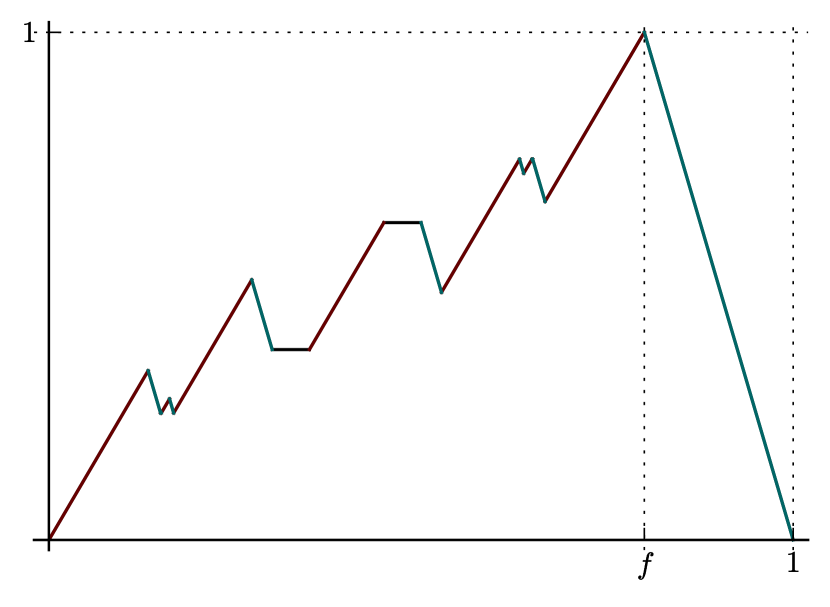
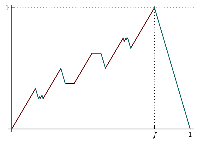
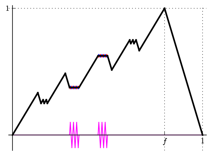
Dey and Wolsey [28, section 2.2, Example 2] give an example where a sequence of continuous piecewise linear extreme functions of type gj_2_slope_repeat converges pointwise to a discontinuous piecewise linear minimal valid function that is not extreme (Figure 10).

$\longrightarrow$

Figure 10. A pointwise limit of extreme functions that is not extreme [28, section 2.2]. Consider the sequence of continuous extreme functions of type gj_2_slope_repeat set up for any $n\in\mathbb{Z}_{+}$ by h = drlm_gj_2_slope_extreme_limit_to_nonextreme(n). For example, $n=3$ (left) and $n=50$ (center). This sequence converges to a non-extreme discontinuous minimal valid function, set up with h = drlm_gj_2_slope_extreme_limit_to_nonextreme() (right). The limit function $\pi$ (black) is shown with two minimal functions $\pi^{1}$ (blue), $\pi^{2}$ (red) such that $\pi=\frac{1}{2}(\pi^{1}+\pi^{2})$.

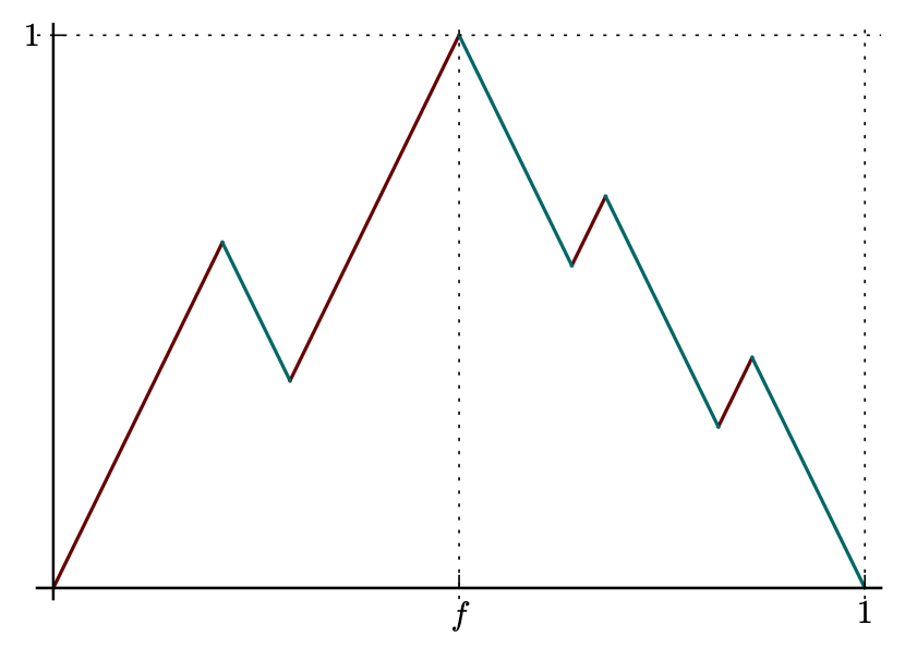
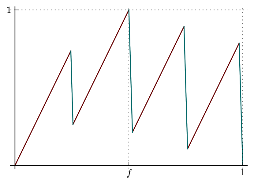
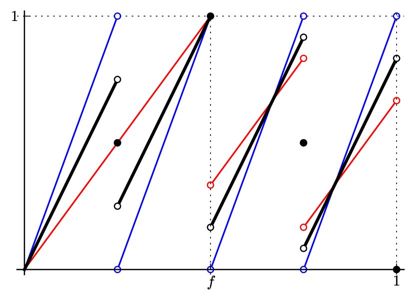
This convergence, of course, is not uniform. One may then ask whether extremality is preserved by stronger notions of convergence. However, even uniform convergence (i.e., convergence in the sense of the space $C(\mathbb{R})$ of continuous functions) or convergence in the sense of the Sobolev space $W^{1,1}_{\mathrm{loc}}(\mathbb{R})$ do not suffice to ensure extremality of the limit function (Figure 11).

Proposition 6.0 (New result $\clubsuit$).

There exists a sequence of continuous extreme functions of type bhk_irrational [15, section 5] that converges uniformly to a continuous non-extreme function of the same type. Further, even the sequence of generalized derivatives converges in the sense of $L^{1}_{\mathrm{loc}}(\mathbb{R})$; thus we have convergence in $W^{1,1}_{\mathrm{loc}}(\mathbb{R})$.

The functions from 6.0 have the intriguing property that extremality depends, in addition to some inequalities in the parameters, on the $\mathbb{Q}$-linear independence of two real parameters [15, Theorems 5.3 and 5.4]. Thus it is easy to construct a sequence of parameters satisfying this condition whose limit is rational, making the limit function non-extreme.

$\longrightarrow$

Figure 11. A uniform limit of extreme functions that is not extreme. The sequence of extreme functions of type bhk_irrational, set up with h = bhk_irrational_extreme_limit_to_rational_nonextreme(n) where $n=1$ (left), $n=2$ (center), … converges to a non-extreme function, set up with h = bhk_irrational_extreme_limit_to_rational_nonextreme() (right). The limit function $\pi$ (black) is shown with two minimal functions $\pi^{1}$ (blue), $\pi^{2}$ (red) such that $\pi=\frac{1}{2}(\pi^{1}+\pi^{2})$ and a scaling of the perturbation function $\bar{\pi}=\pi^{1}-\pi$ (magenta).

6.3. Discontinuous extreme piecewise linear limit functions

Dey and Wolsey [28] give some general conditions under which the limit is indeed extreme. Recall that a function $\pi\in\mathbb{R}^{\mathbb{R}}$ is called piecewise linear (not necessarily continuous) if we can express $\mathbb{R}$ as the union of closed intervals with non-overlapping interiors such that any bounded subset of $\mathbb{R}$ intersects only finitely many intervals, and the function is affine linear over the interior of each interval.

Theorem 6.1 ([28, Theorem 7]).

Let $\pi_{i}\in\mathbb{R}^{\mathbb{R}}$, $i\in\mathbb{N}$ be a sequence of continuous piecewise linear, extreme valid functions for $R_{f}(\mathbb{R},\mathbb{Z})$ and let $\phi$ be the pointwise limit of the sequence $\pi_{i}$, $i\in\mathbb{N}$ such that the following conditions hold:

• $\phi$ is piecewise linear (not necessarily continuous).

• $\phi$ has a finite right derivative at $0$.

• There is a sequence of integers $k_{i}$, $i\in\mathbb{N}$ with $\lim_{i\to\infty}k_{i}=\infty$ such that for each $i\in\mathbb{N}$,

  • $\phi(u)=\pi_{i}(u)$ for all $u\in\frac{1}{k_{i}}\mathbb{Z}$ and

  • the set of nondifferentiable points of $\pi_{i}$ is contained in $\frac{1}{k_{i}}\mathbb{Z}$.

Then $\phi$ is extreme.

The authors of [28] use the above theorem to construct families of discontinuous piecewise linear extreme functions for the single-row infinite group problem; see Table 3 for a list. The use of Theorem 6.1 does not seem to be essential, however; the extremality of all of these functions can also be established by following the algorithm of subsection 7.1.

6.4. Non–piecewise linear extreme limit functions

We now describe a construction based on limits of extreme functions that yields an extreme function that is not piecewise linear. The extremality of this limit function cannot be obtained by an application of Theorem 6.1 since the limit function is not piecewise linear.

This construction is motivated by a conjecture of Gomory and Johnson from 2003 that all facets are piecewise linear [39, section 6.1]. If true, this would justify focusing attention on piecewise linear minimal valid functions, for which we have developed many tools for analysis (see section 3). However, even for $k=1$, this conjecture was disproved by Basu, Conforti, Cornuéjols and Zambelli [12]. We present their counterexample and a brief argument for its extremality.

Remark 6.1.

The arguments for its facetness are almost identical; the only difference is that some technical continuity arguments can be avoided in the proof of extremality because of Lemma 2.1 (iii).

We first define a sequence of valid functions $\psi_{i}\colon\mathbb{R}\rightarrow\mathbb{R}$ that are piecewise linear, and then consider the limit $\psi$ of this sequence, which will be extreme but not piecewise linear.

$\longrightarrow$

Figure 12. First steps ($\psi_{0}=\texttt{\href https://github.com/mkoeppe/infinite-group-relaxation-code/search?q=$, $\psi_{1}$, $\psi_{2}$) in the construction of the continuous non–piecewise linear limit function $\psi=\texttt{\href https://github.com/mkoeppe/infinite-group-relaxation-code/search?q=$.

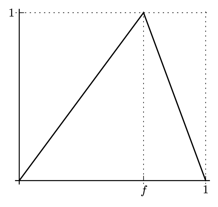
Let $0<f<1$. Consider a geometric sequence of real numbers $\epsilon_{1}>\epsilon_{2}>\dots$ such that $\epsilon_{1}\leq 1-f$ and

$$\mu^{-}=(1-f)+\sum_{i=1}^{+\infty}2^{i-1}\epsilon_{i}\leq 1$$ (17)

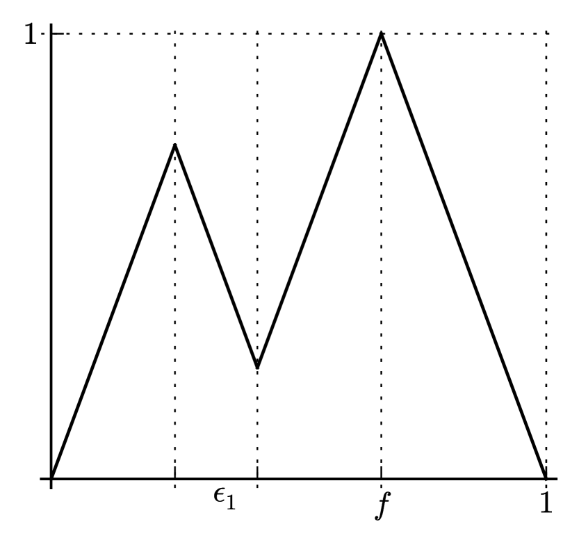
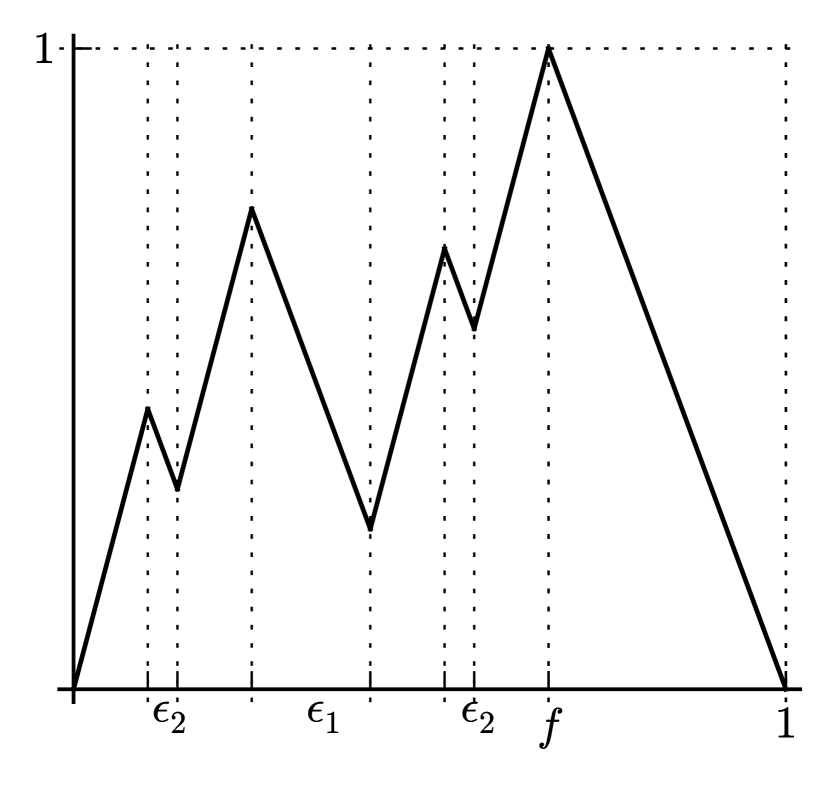
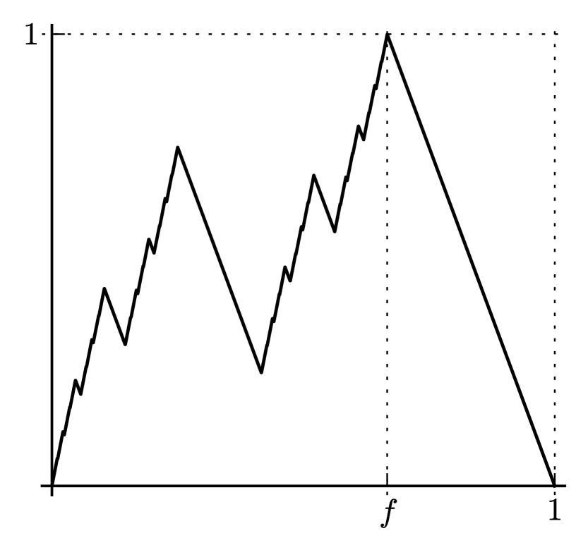
holds. We distinguish two cases: $\mu^{-}<1$ [12] and $\mu^{-}=1$ [45]. An example for the first case is the sequence $\epsilon_{i}=(\frac{1}{4})^{i}f$ for $0<f\leq\frac{4}{5}$; for the second case, $\epsilon_{i}=2(\frac{1}{4})^{i}f$ for $0<f\leq\frac{1}{2}$. Let $\psi_{0}$ be the gmic function with peak at $f$. We construct $\psi_{i+1}$ from $\psi_{i}$ by modifying each segment with positive slope in the graph of $\psi_{i}$ in the manner of the kf_n_step_mir construction [44] as follows. For every inclusion-maximal interval $[a,b]$ where $\psi_{i}$ has constant positive slope we replace the line segment from $(a,\psi_{i}(a))$ to $(b,\psi_{i}(b))$ with the following three segments:

• a positive slope segment connecting $\bigl{(}a,\psi_{i}(a)\bigr{)}$ and $\bigl{(}\frac{(a+b)-\epsilon_{i+1}}{2},\psi_{i}(\frac{a+b}{2})+\frac{\epsilon_{i+1}}{2(1-f)}\bigr{)}$,

• a negative slope segment connecting $\bigl{(}\frac{(a+b)-\epsilon_{i+1}}{2},\psi_{i}(\frac{a+b}{2})+\frac{\epsilon_{i+1}}{2(1-f)}\bigr{)}$ and $\bigl{(}\frac{(a+b)+\epsilon_{i+1}}{2},\psi_{i}(\frac{a+b}{2})-\frac{\epsilon_{i+1}}{2(1-f)}\bigr{)}$,

• a positive slope segment connecting $\bigl{(}\frac{(a+b)+\epsilon_{i+1}}{2},\psi_{i}(\frac{a+b}{2})-\frac{\epsilon_{i+1}}{2(1-f)}\bigr{)}$ and $\bigl{(}b,\psi_{i}(b)\bigr{)}$.

Figure 12 shows the transformation of $\psi_{0}$ to $\psi_{1}$ and $\psi_{1}$ to $\psi_{2}$. Each $\psi_{i}$ is nonnegative, subadditive and satisfies the symmetry condition [12, Lemma 4.5 and Fact 4.6], and thus is a minimal valid function. By construction, the new negative slopes match the existing negative slopes, and the new positive slopes of each function have all the same slope. Thus $\psi_{i}$ is a (continuous piecewise linear) 2-slope function and hence extreme. The functions $\psi_{i}$ are therefore extreme functions by the Gomory–Johnson 2-Slope Theorem (Theorem 2.3).

The function $\psi$ which we show to be extreme but not piecewise linear is defined as the pointwise limit of this sequence of functions, namely

$$\psi(x)=\lim_{i\rightarrow\infty}\psi_{i}(x).$$ (18)

This limit is well defined when (17) holds. In fact, $\psi_{i}$ converges uniformly to $\psi$. Since each $\psi_{i}$ is continuous, this implies that $\psi$ is also continuous. The limit function has the following intriguing properties:

1. By 6.0, $\psi$ is minimal.

2. For each integer $i\geq 0$, define $X^{-}_{i}$ to be the subset of points of $[0,1]$ on which the function $\psi_{i}$ is differentiable with a negative slope. From the construction of $\psi_{i}$, $X^{-}_{i}$ is the union of $2^{i}$ open intervals [12, Fact 4.1]. Furthermore, $X^{-}_{i}\subseteq X^{-}_{i+1}$ for every $i\in\mathbb{N}$. The set $X^{-}\subseteq[0,1]$ defined by $X^{-}=\bigcup_{i=0}^{\infty}X^{-}_{i}$ is thus the set of points over which $\psi$ has negative slope, and it is an open set since it is the union of open intervals. The set $X^{-}$ is dense in $[0,1]$ [12, Fact 5.4]. Its Lebesgue measure is $\mu^{-}$.

3. $\psi$ is not piecewise linear. This is because each $\psi_{i}$ is nonnegative, and therefore so is $\psi$. If $\psi$ is piecewise linear, by definition of continuous piecewise linear functions from subsection 3.1 there exists $0<\epsilon$ such that $\psi$ is affine linear on $[0,\epsilon]$. Since $X^{-}$ is dense, there exists a point from $X^{-}$ in $(0,\epsilon)$ and so $\psi$ has negative slope on this entire segment. But since $\psi(0)=0$, this contradicts the fact that $\psi\geq 0$.

4. The complement $[0,1]\setminus X^{-}$ is a closed set, which does not contain any interval; hence $[0,1]\setminus X^{-}$ is a nowhere dense set. It has Lebesgue measure $\mu^{+}=1-\mu^{-}$. Removing from $[0,1]\setminus X^{-}$ the countably many breakpoints of the negative-slope intervals, we obtain the set $X^{+}=[0,1]\setminus\bigcup_{i=0}^{\infty}\operatorname{cl}X^{-}_{i}$, which is still a nowhere dense set of measure $\mu^{+}$.

5. If $\mu^{-}<1$, the set $X^{+}$ is of positive measure, and thus a fat Cantor set; in this case the derivative of $\psi$ exists for all points in $X^{+}$ and equals the limit of the positive slopes of the functions $\psi_{i}$. Thus $\psi$ is an absolutely continuous, measurable, non–piecewise linear “2-slope function.”

6. On the other hand, if $\mu^{-}=1$, the measure of $X^{+}$ is zero, and so the derivative of $\psi$ equals the negative slopes of the functions $\psi_{i}$ Lebesgue–almost everywhere. Thus $\psi$ is a continuous (but not absolutely continuous), measurable, non–piecewise linear “1-slope function.” This case is discussed in [45].

The proof of extremality of $\psi$ proceeds along the roadmap of subsection 2.3 as follows.

1. Consider any minimal valid functions $\pi^{1},\pi^{2}$ such that $\psi=\frac{\pi^{1}+\pi^{2}}{2}$. Since $\psi$ is affine over the segments in $\operatorname{cl}X^{-}_{i}$, the additivity properties on these segments are inherited by $\pi^{1}$ using a one-dimensional version of 5.1 and Lemma 2.1 (ii).

2. One uses the Interval Lemma (4.0) on $\pi^{1}$ to obtain that $\pi^{1}$ is affine over $X^{-}$, and moreover, since $\pi^{1}(0)=\psi(0)=0$ and $\pi^{1}(f)=\psi(f)=1$, one recursively establishes that $\pi^{1}(x)=\psi(x)$ for all $x\in X^{-}$.

3. Since $X^{-}$ is dense in $[0,1]$, $\psi$ is continuous and $\pi^{1}$ is continuous by Lemma 2.1 (iii) we obtain that $\pi^{1}=\psi$. Therefore, $\pi^{1}=\pi^{2}=\psi$, establishing that $\psi$ is extreme.

We end this section with a conjecture about limits of minimal functions, whose positive resolution would emphasize the importance of piecewise linear functions.

Conjecture 6.1 ([12, Conjecture 6.1]).

Every extreme function (resp. facet) $\pi\colon\mathbb{R}^{k}\to\mathbb{R}$ is either piecewise linear or the limit of a sequence of piecewise linear extreme functions (resp. facets).

7. Algorithmic characterization of extreme functions

In this section we discuss recent algorithmic results for proving piecewise linear functions are either extreme or not extreme for the infinite group problem $R_{\mathchoice{\mbox{\boldmath$\displaystyle\bf f$}}{\mbox{\boldmath$\textstyle\bf f$}}{\mbox{\boldmath$\scriptstyle\bf f$}}{\mbox{\boldmath$\scriptscriptstyle\bf f$}}}(\mathbb{R}^{k},\mathbb{Z}^{k})$. In [15], the first algorithmic test for extremality was given for the single-row infinite group problem $R_{f}(\mathbb{R},\mathbb{Z})$, followed by an extension to two-row infinite group problem $R_{\mathchoice{\mbox{\boldmath$\displaystyle\bf f$}}{\mbox{\boldmath$\textstyle\bf f$}}{\mbox{\boldmath$\scriptstyle\bf f$}}{\mbox{\boldmath$\scriptscriptstyle\bf f$}}}(\mathbb{R}^{2},\mathbb{Z}^{2})$ in [16]. We summarize these algorithmic ideas here in two lights. We will first discuss a general procedure to test for extremality and then in section 8 discuss specific classes of functions that have relations to finite group problems where extremality can be tested easily using linear algebra.

7.1. General procedure outline

We will outline here a general procedure for testing extremality of a continuous piecewise linear function $\pi\colon\mathbb{R}^{k}\to\mathbb{R}$ defined on a polyhedral complex $\mathcal{P}$. Similar techniques may apply to testing extremality and even facetness of discontinuous piecewise linear functions as well.

Let $E=E(\pi)$. Recall that $\pi$ is not extreme if and only if there exists a nontrivial function $\bar{\pi}$ such that $\pi\pm\bar{\pi}$ is minimal. From Lemma 2.1 parts (i) and (ii) it follows that $\pi$ is not extreme if and only if there exists a nontrivial continuous function $\bar{\pi}\in\bar{\Pi}^{E}(\mathbb{R}^{k},\mathbb{Z}^{k})$ such that $\pi\pm\bar{\pi}$ is minimal.

Let $\mathcal{T}$ be a triangulation of $\mathbb{R}^{k}$ that satisfies the hypotheses of Lemma 3.3, i.e., there exists $q\in\mathbb{N}$ such that $\operatorname{vert}(\mathcal{T})=\tfrac{1}{q}\mathbb{Z}^{k}$ and $p_{i}(\operatorname{vert}(\Delta\mathcal{T}))\subseteq\tfrac{1}{q}\mathbb{Z}^{k}$ for $i=1,2,3$ and ${\mathchoice{\mbox{\boldmath$\displaystyle\bf f$}}{\mbox{\boldmath$\textstyle\bf f$}}{\mbox{\boldmath$\scriptstyle\bf f$}}{\mbox{\boldmath$\scriptscriptstyle\bf f$}}}\in\tfrac{1}{q}\mathbb{Z}^{k}$. The following algorithmic ideas are based on the decomposition in Lemma 3.3 part (2) of perturbations $\bar{\pi}\in\bar{\Pi}^{E}(\mathbb{R}^{k},\mathbb{Z}^{k})$ into $\bar{\pi}=\bar{\pi}_{\mathcal{T}}+\bar{\pi}_{\mathrm{zero}(\mathcal{T})}$ with $\bar{\pi}_{\mathcal{T}}\in\bar{\Pi}^{E}_{\mathcal{T}}(\mathbb{R}^{k},\mathbb{Z}^{k})$ and $\bar{\pi}_{\mathrm{zero}(\mathcal{T})}\in\bar{\Pi}^{E}_{\mathrm{zero}(\mathcal{T})}(\mathbb{R}^{k},\mathbb{Z}^{k})$. Since $\bar{\pi}$ and $\bar{\pi}_{\mathcal{T}}$ are continuous, $\bar{\pi}_{\mathrm{zero}(\mathcal{T})}$ is also continuous.

7.1.1. Finite-dimensional linear algebra for $\bar{\Pi}^{E}_{\mathcal{T}}(\mathbb{R}^{k},\mathbb{Z}^{k})$

We begin by looking for a perturbation function in $\bar{\Pi}^{E}_{\mathcal{T}}(\mathbb{R}^{k},\mathbb{Z}^{k})$. By Lemma 3.3, $\bar{\pi}\in\bar{\Pi}^{E}_{\mathcal{T}}(\mathbb{R}^{k},\mathbb{Z}^{k})$ if and only if $\bar{\pi}|_{\frac{1}{q}\mathbb{Z}^{k}}\in\bar{\Pi}^{E^{\prime}}(\tfrac{1}{q}\mathbb{Z}^{k},\mathbb{Z}^{k})$ where $E^{\prime}=E(\pi)\cap\tfrac{1}{q}\mathbb{Z}^{k}$. Thus we consider the linear system $\bar{\Pi}^{E^{\prime}}(\tfrac{1}{q}\mathbb{Z}^{k},\mathbb{Z}^{k})$, which is finite-dimensional if we identify the variables $\bar{\pi}({\mathchoice{\mbox{\boldmath$\displaystyle\bf x$}}{\mbox{\boldmath$\textstyle\bf x$}}{\mbox{\boldmath$\scriptstyle\bf x$}}{\mbox{\boldmath$\scriptscriptstyle\bf x$}}})$ and $\bar{\pi}({\mathchoice{\mbox{\boldmath$\displaystyle\bf x$}}{\mbox{\boldmath$\textstyle\bf x$}}{\mbox{\boldmath$\scriptstyle\bf x$}}{\mbox{\boldmath$\scriptscriptstyle\bf x$}}}+{\mathchoice{\mbox{\boldmath$\displaystyle\bf t$}}{\mbox{\boldmath$\textstyle\bf t$}}{\mbox{\boldmath$\scriptstyle\bf t$}}{\mbox{\boldmath$\scriptscriptstyle\bf t$}}})$ for all ${\mathchoice{\mbox{\boldmath$\displaystyle\bf t$}}{\mbox{\boldmath$\textstyle\bf t$}}{\mbox{\boldmath$\scriptstyle\bf t$}}{\mbox{\boldmath$\scriptscriptstyle\bf t$}}}\in\mathbb{Z}^{k}$. Hence, this is a finite-dimensional linear system and any nontrivial solution can be computed by analyzing the null space of this system. If such a nontrivial solution exists, it can be interpolated to a piecewise linear function $\bar{\pi}\in\bar{\Pi}^{E}_{\mathcal{T}}(\mathbb{R}^{k},\mathbb{Z}^{k})$ because $\mathcal{T}$ is a triangulation of $\mathbb{R}^{k}$ that satisfies the hypotheses of Lemma 3.3, and so by Theorem 3.3 $\pi$ is not extreme. This is demonstrated in Figure 3 for the case of $\mathcal{T}=\mathcal{P}=\mathcal{P}_{\frac{1}{q}\mathbb{Z}}$ where a perturbation is found on the complex $\mathcal{T}$.

Otherwise we have that $\bar{\Pi}^{E}_{\mathcal{T}}(\mathbb{R}^{k},\mathbb{Z}^{k})=\{0\}$. This scenario is depicted in Figure 14 where $\bar{\Pi}^{E^{\prime}}_{\mathcal{P}_{\frac{1}{q}\mathbb{Z}}}(\tfrac{1}{q}\mathbb{Z},\mathbb{Z})=\{0\}$ with $E^{\prime}=E(\pi)\cap\tfrac{1}{q}\mathbb{Z}^{2}$.

7.1.2. Projections and additivity for $\bar{\Pi}^{E}_{\mathrm{zero}(\mathcal{T})}(\mathbb{R}^{k},\mathbb{Z}^{k})$

From Lemma 3.3, any $\bar{\pi}\in\bar{\Pi}^{E}_{\mathrm{zero}(\mathcal{T})}(\mathbb{R}^{k},\mathbb{Z}^{k})$ satisfies $\bar{\pi}|_{\frac{1}{q}\mathbb{Z}^{k}}\equiv 0$.

We consider full-dimensional faces $F\in E(\pi,\mathcal{P})$. By Corollary 4.4, these full-dimensional faces imply that any $\bar{\pi}\in\bar{\Pi}^{E}_{\mathrm{zero}(\mathcal{T})}(\mathbb{R}^{k},\mathbb{Z}^{k})$ is affine on the projections $p_{1}(F),p_{2}(F)$, and $p_{3}(F)$. If a projection $p_{i}(F)$ contains $k+1$ affinely independent points in $\frac{1}{q}\mathbb{Z}^{k}$, then we conclude that $\bar{\pi}|_{p_{i}(F)}\equiv 0$ on this projection. This is because $\bar{\pi}|_{\frac{1}{q}\mathbb{Z}^{k}}\equiv 0$. Therefore, we learn certain polyhedral regions where $\bar{\pi}$ vanishes and we record these.

In the next step, we consider any faces $F$ of $E(\pi,\mathcal{P})$ such that two of $p_{1}(F),p_{2}(F),p_{3}(F)$ are full-dimensional and one is zero-dimensional. In particular, if one of these full-dimensional projections intersects a region where $\bar{\pi}$ is zero, then that property is transferred to the other full-dimensional projection. For example, the relations $\pi({\mathchoice{\mbox{\boldmath$\displaystyle\bf x$}}{\mbox{\boldmath$\textstyle\bf x$}}{\mbox{\boldmath$\scriptstyle\bf x$}}{\mbox{\boldmath$\scriptscriptstyle\bf x$}}})+\pi({\mathchoice{\mbox{\boldmath$\displaystyle\bf t$}}{\mbox{\boldmath$\textstyle\bf t$}}{\mbox{\boldmath$\scriptstyle\bf t$}}{\mbox{\boldmath$\scriptscriptstyle\bf t$}}})=\pi({\mathchoice{\mbox{\boldmath$\displaystyle\bf x$}}{\mbox{\boldmath$\textstyle\bf x$}}{\mbox{\boldmath$\scriptstyle\bf x$}}{\mbox{\boldmath$\scriptscriptstyle\bf x$}}}+{\mathchoice{\mbox{\boldmath$\displaystyle\bf t$}}{\mbox{\boldmath$\textstyle\bf t$}}{\mbox{\boldmath$\scriptstyle\bf t$}}{\mbox{\boldmath$\scriptscriptstyle\bf t$}}})$ for all ${\mathchoice{\mbox{\boldmath$\displaystyle\bf x$}}{\mbox{\boldmath$\textstyle\bf x$}}{\mbox{\boldmath$\scriptstyle\bf x$}}{\mbox{\boldmath$\scriptscriptstyle\bf x$}}}\in I$ corresponds to the face $F=F(I,\{{\mathchoice{\mbox{\boldmath$\displaystyle\bf t$}}{\mbox{\boldmath$\textstyle\bf t$}}{\mbox{\boldmath$\scriptstyle\bf t$}}{\mbox{\boldmath$\scriptscriptstyle\bf t$}}}\},I+\{{\mathchoice{\mbox{\boldmath$\displaystyle\bf t$}}{\mbox{\boldmath$\textstyle\bf t$}}{\mbox{\boldmath$\scriptstyle\bf t$}}{\mbox{\boldmath$\scriptscriptstyle\bf t$}}}\})$ where $p_{1}(F)=I$, $p_{2}(F)=\{{\mathchoice{\mbox{\boldmath$\displaystyle\bf t$}}{\mbox{\boldmath$\textstyle\bf t$}}{\mbox{\boldmath$\scriptstyle\bf t$}}{\mbox{\boldmath$\scriptscriptstyle\bf t$}}}\}$, $p_{3}(F)=I+\{{\mathchoice{\mbox{\boldmath$\displaystyle\bf t$}}{\mbox{\boldmath$\textstyle\bf t$}}{\mbox{\boldmath$\scriptstyle\bf t$}}{\mbox{\boldmath$\scriptscriptstyle\bf t$}}}\}$. Hence, if $I$ is full-dimensional in $\mathbb{R}^{k}$ then $I+\{{\mathchoice{\mbox{\boldmath$\displaystyle\bf t$}}{\mbox{\boldmath$\textstyle\bf t$}}{\mbox{\boldmath$\scriptstyle\bf t$}}{\mbox{\boldmath$\scriptscriptstyle\bf t$}}}\}$ is full-dimensional in $\mathbb{R}^{k}$. In this way the function values of $\bar{\pi}$ in $I+\{{\mathchoice{\mbox{\boldmath$\displaystyle\bf t$}}{\mbox{\boldmath$\textstyle\bf t$}}{\mbox{\boldmath$\scriptstyle\bf t$}}{\mbox{\boldmath$\scriptscriptstyle\bf t$}}}\}$ are dependent on the function values on $I$. For example, if we know that $\bar{\pi}$ is affine over $I$, then it is also affine over $I+\{{\mathchoice{\mbox{\boldmath$\displaystyle\bf t$}}{\mbox{\boldmath$\textstyle\bf t$}}{\mbox{\boldmath$\scriptstyle\bf t$}}{\mbox{\boldmath$\scriptscriptstyle\bf t$}}}\}$. This is the key step in this procedure. We continue transferring properties until no new affine properties are discovered.

If the procedure terminates, it may either show that $\bar{\pi}\equiv 0$, in which case $\pi$ is extreme. Otherwise, we hope to find a perturbation function $\bar{\pi}$ that shows that $\pi$ is not extreme. In fact, in certain cases, we can find a $\bar{\pi}$ that is piecewise linear on a refinement of $\mathcal{T}$. Showing termination of this procedure is non-trivial and it is an open question under what conditions this procedure is guaranteed to terminate. Subsections 7.2 and 7.3 discuss cases in which the procedure provably terminates.

The above procedure only considers certain faces of $E(\pi,\mathcal{P})$. Other faces of $E(\pi,\mathcal{P})$, as shown in Theorem 4.3, establish other affine properties about $\bar{\pi}$, but not necessarily full-dimensional affine properties. These properties can sometimes combine to create full-dimensional affine properties. This effect is investigated in the forthcoming paper [17] for the case of the two-row problem and general continuous piecewise linear functions over the complex $\mathcal{P}_{q}$.

7.2. One-row case with rational breakpoints

We will consider the one-dimensional polyhedral complex $\mathcal{P}_{B}$ for $B=\frac{1}{q}\mathbb{Z}\cap[0,1)$ as defined in Example 3.0; we will call this complex $\mathcal{P}_{\frac{1}{q}\mathbb{Z}}$. Therefore, we consider piecewise linear functions (possibly discontinuous) with breakpoints in $\frac{1}{q}\mathbb{Z}$.

Theorem 7.1 ([15, Theorem 1.3]).

Consider the following problem.

Given a minimal valid function $\pi$ for $R_{f}(\mathbb{R},\mathbb{Z})$ that is piecewise linear with a set of rational breakpoints with the least common denominator $q$, decide if $\pi$ is extreme or not.

There exists an algorithm for this problem whose running time is bounded by a polynomial in $q$.

Since the above algorithm is polynomial in the least common denominator $q$, it is only a pseudo-polynomial time algorithm.

Open question 7.1.

Does there exist a polynomial time algorithm to determine extremality of piecewise linear functions for $R_{f}(\mathbb{R},\mathbb{Z})$?

A more general version of the above algorithm is implemented in [41] for the case of piecewise linear functions, which are allowed to be continuous or discontinuous, and whose data may be algebraic irrational numbers. The implementation will be described in more detail in a forthcoming article.

7.3. Two-row case using a standard triangulation of $\mathbb{R}^{2}$

For the case of the standard triangulations $\mathcal{P}_{q}$ of $\mathbb{R}^{2}$ (3.0), [14, 16] describe an algorithm of the above scheme for a special class of piecewise linear functions over this complex, which are said to be diagonally constrained.

Let

$$A=\begin{bmatrix}1&-1&0&0&1&-1\\ 0&0&1&-1&1&-1\end{bmatrix}^{T}.$$

Then for every face $I\in\mathcal{P}_{q}$, there exists a vector $\mathchoice{\mbox{\boldmath$\displaystyle\bf b$}}{\mbox{\boldmath$\textstyle\bf b$}}{\mbox{\boldmath$\scriptstyle\bf b$}}{\mbox{\boldmath$\scriptscriptstyle\bf b$}}\in\frac{1}{q}\mathbb{Z}^{6}$ such that $I=\{\,{\mathchoice{\mbox{\boldmath$\displaystyle\bf x$}}{\mbox{\boldmath$\textstyle\bf x$}}{\mbox{\boldmath$\scriptstyle\bf x$}}{\mbox{\boldmath$\scriptscriptstyle\bf x$}}}\mid A{\mathchoice{\mbox{\boldmath$\displaystyle\bf x$}}{\mbox{\boldmath$\textstyle\bf x$}}{\mbox{\boldmath$\scriptstyle\bf x$}}{\mbox{\boldmath$\scriptscriptstyle\bf x$}}}\leq\mathchoice{\mbox{\boldmath$\displaystyle\bf b$}}{\mbox{\boldmath$\textstyle\bf b$}}{\mbox{\boldmath$\scriptstyle\bf b$}}{\mbox{\boldmath$\scriptscriptstyle\bf b$}}\,\}.$ Furthermore, for every vector $\mathchoice{\mbox{\boldmath$\displaystyle\bf b$}}{\mbox{\boldmath$\textstyle\bf b$}}{\mbox{\boldmath$\scriptstyle\bf b$}}{\mbox{\boldmath$\scriptscriptstyle\bf b$}}\in\frac{1}{q}\mathbb{Z}^{6}$, the set $\{\,{\mathchoice{\mbox{\boldmath$\displaystyle\bf x$}}{\mbox{\boldmath$\textstyle\bf x$}}{\mbox{\boldmath$\scriptstyle\bf x$}}{\mbox{\boldmath$\scriptscriptstyle\bf x$}}}\mid A{\mathchoice{\mbox{\boldmath$\displaystyle\bf x$}}{\mbox{\boldmath$\textstyle\bf x$}}{\mbox{\boldmath$\scriptstyle\bf x$}}{\mbox{\boldmath$\scriptscriptstyle\bf x$}}}\leq\mathchoice{\mbox{\boldmath$\displaystyle\bf b$}}{\mbox{\boldmath$\textstyle\bf b$}}{\mbox{\boldmath$\scriptstyle\bf b$}}{\mbox{\boldmath$\scriptscriptstyle\bf b$}}\,\}$ is a union of faces of $\mathcal{P}_{q}$ (possibly empty), since each inequality corresponds to a hyperplane in the arrangement $\mathcal{H}_{q}$. The matrix $A$ is totally unimodular and this fact plays a key role in proving the following lemma.

Lemma 7.1.

Let $F\in\Delta\mathcal{P}_{q}$. Then the projections $p_{1}(F)$, $p_{2}(F)$, and $p_{3}(F)$ are faces in the complex $\mathcal{P}_{q}$. In particular, let $({\mathchoice{\mbox{\boldmath$\displaystyle\bf x$}}{\mbox{\boldmath$\textstyle\bf x$}}{\mbox{\boldmath$\scriptstyle\bf x$}}{\mbox{\boldmath$\scriptscriptstyle\bf x$}}},{\mathchoice{\mbox{\boldmath$\displaystyle\bf y$}}{\mbox{\boldmath$\textstyle\bf y$}}{\mbox{\boldmath$\scriptstyle\bf y$}}{\mbox{\boldmath$\scriptscriptstyle\bf y$}}})$ be a vertex of $\Delta\mathcal{P}_{q}$. Then ${\mathchoice{\mbox{\boldmath$\displaystyle\bf x$}}{\mbox{\boldmath$\textstyle\bf x$}}{\mbox{\boldmath$\scriptstyle\bf x$}}{\mbox{\boldmath$\scriptscriptstyle\bf x$}}},{\mathchoice{\mbox{\boldmath$\displaystyle\bf y$}}{\mbox{\boldmath$\textstyle\bf y$}}{\mbox{\boldmath$\scriptstyle\bf y$}}{\mbox{\boldmath$\scriptscriptstyle\bf y$}}}$ are vertices of the complex $\mathcal{P}_{q}$, i.e., ${\mathchoice{\mbox{\boldmath$\displaystyle\bf x$}}{\mbox{\boldmath$\textstyle\bf x$}}{\mbox{\boldmath$\scriptstyle\bf x$}}{\mbox{\boldmath$\scriptscriptstyle\bf x$}}},{\mathchoice{\mbox{\boldmath$\displaystyle\bf y$}}{\mbox{\boldmath$\textstyle\bf y$}}{\mbox{\boldmath$\scriptstyle\bf y$}}{\mbox{\boldmath$\scriptscriptstyle\bf y$}}}\in\frac{1}{q}\mathbb{Z}^{2}$.

Extremality is more easily studied if we restrict ourselves to a setting determined by the types of faces $F\in E_{\max{}}(\pi,\mathcal{P}_{q})$. Recall that

$$E_{\max{}}(\pi,\mathcal{P}_{q})=\left\{\,F\in E(\pi,\mathcal{P}_{q})\,\mid\,F\text{ is a maximal face by set inclusion in }E(\pi,\mathcal{P}_{q})\,\right\}.$$

Definition 7.1.

A continuous piecewise linear function $\pi$ on $\mathcal{P}_{q}$ is called diagonally constrained if for all $F\in E_{\max{}}(\pi,\mathcal{P}_{q})$ and $i=1,2,3$, the projection $p_{i}(F)$ is either a vertex, diagonal edge, or triangle from the complex $\mathcal{P}_{q}$.

The properties in Lemma 7.1 provide an easy method to compute $E(\pi,\mathcal{P}_{q})$ and test if a function is diagonally constrained by using simple arithmetic and set membership operations on vertices of $\mathcal{P}_{q}$.

Figure 13. A minimal valid, continuous, piecewise linear function over the polyhedral complex $\mathcal{P}_{5}$, which is diagonally constrained (subsection 7.3). Left, the three-dimensional plot of the function on $D=[0,1]^{2}$. Right, the complex $\mathcal{P}_{5}$, restricted to $D$ and colored according to slopes to match the 3-dimensional plot, and decorated with values $v$ at each vertex of $\mathcal{P}_{5}$ where the function takes value $\tfrac{v}{4}$.

Example 7.1.

Figure 13 shows the complex $\mathcal{P}_{5}$ with an example of a minimal valid continuous piecewise linear function on $\mathcal{P}_{5}$ with ${\mathchoice{\mbox{\boldmath$\displaystyle\bf f$}}{\mbox{\boldmath$\textstyle\bf f$}}{\mbox{\boldmath$\scriptstyle\bf f$}}{\mbox{\boldmath$\scriptscriptstyle\bf f$}}}={\bigl{(}\begin{smallmatrix}2/5\\ 2/5\end{smallmatrix}\bigr{)}}$ that is periodic modulo $\mathbb{Z}^{2}$. Note that, due the periodicity of the function modulo $\mathbb{Z}^{2}$, the values of the function on the left and the right edge (and likewise on the bottom and the top edge) of $D=[0,1]^{2}$ match.

It can be checked that no relations appearing in the list of all maximal additive faces involve a vertical or horizontal edge; thus, the function is diagonally constrained. See [16, sections LABEL:equi3:s:geometry-Pq and LABEL:equi3:subsection:maximal-faces].

Theorem 7.2 ([16, LABEL:equi3:thm:main]).

Consider the following problem.

Given a minimal valid function $\pi$ for $R_{{\mathchoice{\mbox{\boldmath$\displaystyle\bf f$}}{\mbox{\boldmath$\textstyle\bf f$}}{\mbox{\boldmath$\scriptstyle\bf f$}}{\mbox{\boldmath$\scriptscriptstyle\bf f$}}}}(\mathbb{R}^{2},\mathbb{Z}^{2})$ that is piecewise linear continuous on $\mathcal{P}_{q}$ and diagonally constrained with ${\mathchoice{\mbox{\boldmath$\displaystyle\bf f$}}{\mbox{\boldmath$\textstyle\bf f$}}{\mbox{\boldmath$\scriptstyle\bf f$}}{\mbox{\boldmath$\scriptscriptstyle\bf f$}}}\in\operatorname{vert}(\mathcal{P}_{q})$, decide if $\pi$ is extreme.

There exists an algorithm for this problem whose running time is bounded by a polynomial in $q$.

As before, this algorithm is only a pseudo-polynomial time algorithm.

Open question 7.2.

For any fixed $k$, does there exist a polynomial time algorithm to determine extremality of piecewise linear functions for $R_{\mathchoice{\mbox{\boldmath$\displaystyle\bf f$}}{\mbox{\boldmath$\textstyle\bf f$}}{\mbox{\boldmath$\scriptstyle\bf f$}}{\mbox{\boldmath$\scriptscriptstyle\bf f$}}}(\mathbb{R}^{k},\mathbb{Z}^{k})$?

Unlike in the one-row problem, even with all rational input, no algorithm is known for determining extremality of piecewise linear functions for $R_{\mathchoice{\mbox{\boldmath$\displaystyle\bf f$}}{\mbox{\boldmath$\textstyle\bf f$}}{\mbox{\boldmath$\scriptstyle\bf f$}}{\mbox{\boldmath$\scriptscriptstyle\bf f$}}}(\mathbb{R}^{k},\mathbb{Z}^{k})$ for $k\geq 3$ and, as mentioned in Theorem 7.2, only for certain cases is an algorithm known for $k=2$.

8. Algorithm using restriction to finite group problems

In this section, we discuss connections between infinite group problems and finite group problems. We begin with a discussion of testing extremality for finite group problems. Later we show that in certain settings, a function is extreme for an infinite group problem if and only if its restriction to a finite group is extreme for the finite group problem. Hence, this connection provides an alternative algorithm from those described in section 7 for testing extremality and facetness.

8.1. Algorithm for finite group problem

When $S$ has finite index in $G$, we call $R_{\mathchoice{\mbox{\boldmath$\displaystyle\bf f$}}{\mbox{\boldmath$\textstyle\bf f$}}{\mbox{\boldmath$\scriptstyle\bf f$}}{\mbox{\boldmath$\scriptscriptstyle\bf f$}}}(G,S)$ a finite group problem. As we noted in Remark 2.0, $R_{\mathchoice{\mbox{\boldmath$\displaystyle\bf f$}}{\mbox{\boldmath$\textstyle\bf f$}}{\mbox{\boldmath$\scriptstyle\bf f$}}{\mbox{\boldmath$\scriptscriptstyle\bf f$}}}(G,S)$ and $R_{\mathchoice{\mbox{\boldmath$\displaystyle\bf f$}}{\mbox{\boldmath$\textstyle\bf f$}}{\mbox{\boldmath$\scriptstyle\bf f$}}{\mbox{\boldmath$\scriptscriptstyle\bf f$}}}(G/S,0)$ are closely related by aggregation of variables, and it is convenient to study the finite-dimensional problem $R_{\bar{\mathchoice{\mbox{\boldmath$\displaystyle\bf f$}}{\mbox{\boldmath$\textstyle\bf f$}}{\mbox{\boldmath$\scriptstyle\bf f$}}{\mbox{\boldmath$\scriptscriptstyle\bf f$}}}}(G/S,0)$. The fundamental theorem of finitely generated abelian groups shows that $G/S\cong(\tfrac{1}{q_{1}}\mathbb{Z}\times\dots\times\tfrac{1}{q_{k}}\mathbb{Z})/\mathbb{Z}^{k}$ for some $q_{i}\in\mathbb{N}$ for $i=1,\dots,k$. Therefore, it suffices to consider $G=\tfrac{1}{q_{1}}\mathbb{Z}\times\dots\times\tfrac{1}{q_{k}}\mathbb{Z}$ and $S=\mathbb{Z}^{k}$ where $q_{i}\in\mathbb{N}$. In the case of one row, $G/S=\tfrac{1}{q_{1}}\mathbb{Z}/\mathbb{Z}\cong\mathbb{Z}/q_{1}\mathbb{Z}$ is a cyclic group. Cyclic group problems were originally studied by Gomory [35] and have been the subject of many later studies. See [48] for an excellent survey on these results.

The set of minimal valid functions $\pi\colon G/S\to\mathbb{R}$ is a (finite-dimensional) convex polytope [35]. Extreme functions are thus extreme points of this polytope. As we noted in subsubsection 2.2.4, standard polyhedral theory reveals that extreme functions are equivalent to weak facets and facets. Furthermore, extreme points of polytopes are characterized by points where the tight inequalities are of full rank. Therefore, testing extremality of a function for a finite group problem can be done with simple linear algebra.

Note that there is a bijection between the minimal valid functions of $R_{\mathchoice{\mbox{\boldmath$\displaystyle\bf f$}}{\mbox{\boldmath$\textstyle\bf f$}}{\mbox{\boldmath$\scriptstyle\bf f$}}{\mbox{\boldmath$\scriptscriptstyle\bf f$}}}(G,S)$ and minimal valid functions for $R_{\bar{\mathchoice{\mbox{\boldmath$\displaystyle\bf f$}}{\mbox{\boldmath$\textstyle\bf f$}}{\mbox{\boldmath$\scriptstyle\bf f$}}{\mbox{\boldmath$\scriptscriptstyle\bf f$}}}}(G/S,0)$. This is because minimal valid functions for $R_{\mathchoice{\mbox{\boldmath$\displaystyle\bf f$}}{\mbox{\boldmath$\textstyle\bf f$}}{\mbox{\boldmath$\scriptstyle\bf f$}}{\mbox{\boldmath$\scriptscriptstyle\bf f$}}}(G,S)$ are $S$-periodic functions by Theorem 2.1. Hence the extremality test translates into the following statement about $\bar{\Pi}^{E(\pi)}(G,\mathbb{Z}^{k})$.

Theorem 8.1.

Let $G=\tfrac{1}{q_{1}}\mathbb{Z}\times\dots\times\tfrac{1}{q_{k}}\mathbb{Z}$ and let ${\mathchoice{\mbox{\boldmath$\displaystyle\bf f$}}{\mbox{\boldmath$\textstyle\bf f$}}{\mbox{\boldmath$\scriptstyle\bf f$}}{\mbox{\boldmath$\scriptscriptstyle\bf f$}}}\in G$. Let $\pi\colon G\to\mathbb{R}$ be a minimal valid function for $R_{\mathchoice{\mbox{\boldmath$\displaystyle\bf f$}}{\mbox{\boldmath$\textstyle\bf f$}}{\mbox{\boldmath$\scriptstyle\bf f$}}{\mbox{\boldmath$\scriptscriptstyle\bf f$}}}(G,\mathbb{Z}^{k})$. Then $\pi$ is extreme if and only if $\bar{\Pi}^{E}(G,\mathbb{Z}^{k})=\{0\}$ where $E=E(\pi)$.

For any discrete group $G\supseteq\mathbb{Z}^{k}$ and subgroup $G^{\prime}$, the set $R_{\mathchoice{\mbox{\boldmath$\displaystyle\bf f$}}{\mbox{\boldmath$\textstyle\bf f$}}{\mbox{\boldmath$\scriptstyle\bf f$}}{\mbox{\boldmath$\scriptscriptstyle\bf f$}}}(G^{\prime}/\mathbb{Z}^{k},0)$ is a face of the polyhedron $R_{\mathchoice{\mbox{\boldmath$\displaystyle\bf f$}}{\mbox{\boldmath$\textstyle\bf f$}}{\mbox{\boldmath$\scriptstyle\bf f$}}{\mbox{\boldmath$\scriptscriptstyle\bf f$}}}(G/\mathbb{Z}^{k},0)$. This observation implies the following theorem via the above bijection.

Theorem 8.2.

Let $G=\tfrac{1}{q_{1}}\mathbb{Z}\times\dots\times\tfrac{1}{q_{k}}\mathbb{Z}$, let $G^{\prime}$ be any subgroup of $G$, and let ${\mathchoice{\mbox{\boldmath$\displaystyle\bf f$}}{\mbox{\boldmath$\textstyle\bf f$}}{\mbox{\boldmath$\scriptstyle\bf f$}}{\mbox{\boldmath$\scriptscriptstyle\bf f$}}}\in G^{\prime}$. Let $\pi\colon G\to\mathbb{R}$.

1. If $\pi$ is minimal for $R_{\mathchoice{\mbox{\boldmath$\displaystyle\bf f$}}{\mbox{\boldmath$\textstyle\bf f$}}{\mbox{\boldmath$\scriptstyle\bf f$}}{\mbox{\boldmath$\scriptscriptstyle\bf f$}}}(G,\mathbb{Z}^{k})$, then $\pi$ is minimal for $R_{\mathchoice{\mbox{\boldmath$\displaystyle\bf f$}}{\mbox{\boldmath$\textstyle\bf f$}}{\mbox{\boldmath$\scriptstyle\bf f$}}{\mbox{\boldmath$\scriptscriptstyle\bf f$}}}(G^{\prime},\mathbb{Z}^{k})$.

2. If $\pi$ is extreme for $R_{\mathchoice{\mbox{\boldmath$\displaystyle\bf f$}}{\mbox{\boldmath$\textstyle\bf f$}}{\mbox{\boldmath$\scriptstyle\bf f$}}{\mbox{\boldmath$\scriptscriptstyle\bf f$}}}(G,\mathbb{Z}^{k})$, then $\pi$ is extreme for $R_{\mathchoice{\mbox{\boldmath$\displaystyle\bf f$}}{\mbox{\boldmath$\textstyle\bf f$}}{\mbox{\boldmath$\scriptstyle\bf f$}}{\mbox{\boldmath$\scriptscriptstyle\bf f$}}}(G^{\prime},\mathbb{Z}^{k})$.

8.2. Restriction and interpolation in the one-row problem

Gomory and Johnson devised the infinite group problem as a way to study the finite group problem. They studied interpolations of valid functions of the finite group problems $R_{f}(\tfrac{1}{q}\mathbb{Z},\mathbb{Z})$ in order to connect the problems, but they never completed this program. Due to the ease of testing extremality in the finite group problems, having this connection is useful for algorithms. We encapsulate their results on this connection in the following theorem.

Theorem 8.3 ([37]).

Let $\pi$ be a continuous piecewise linear function with breakpoints in $\tfrac{1}{q}\mathbb{Z}$ for some $q\in\mathbb{Z}_{+}$ and let $f\in\tfrac{1}{q}\mathbb{Z}$. Then the following hold:

1. $\pi$ is minimal for $R_{f}(\mathbb{R},\mathbb{Z})$ if and only if $\pi_{\frac{1}{q}\mathbb{Z}}$ is minimal for $R_{f}(\tfrac{1}{q}\mathbb{Z},\mathbb{Z})$.

2. If $\pi$ is extreme for $R_{f}(\mathbb{R},\mathbb{Z})$, then $\pi|_{\frac{1}{q}\mathbb{Z}}$ is extreme for $R_{f}(\tfrac{1}{q}\mathbb{Z},\mathbb{Z})$.

Part (1) shows that minimality can be tested on just points in $\tfrac{1}{q}\mathbb{Z}$, while part (2) yields a method of proving a function is not extreme. That is, if $\pi|_{\frac{1}{q}\mathbb{Z}}$ is not extreme for $R_{f}(\tfrac{1}{q}\mathbb{Z},\mathbb{Z})$, then $\pi$ is not extreme for $R_{f}(\mathbb{R},\mathbb{Z})$. However, it is not true in general that if $\pi|_{\frac{1}{q}\mathbb{Z}}$ is extreme for $R_{f}(\frac{1}{q}\mathbb{Z},\mathbb{Z})$, then $\pi$ is extreme for $R_{f}(\mathbb{R},\mathbb{Z})$. See Figure 14 for an example. To obtain such a characterization, it turns out that we must restrict to a finer grid. The first result in this direction of relating the infinite and the finite group problems appeared in [28]; we state it in our notation.

Theorem 8.4 ([28, Theorem 6]).

Let $\pi$ be a piecewise linear minimal valid function for $R_{f}(\mathbb{R},\mathbb{Z})$ with set $B$ of rational breakpoints with the least common denominator $q$. Then $\pi$ is extreme if and only if the restriction $\pi|_{\frac{1}{2^{n}q}\mathbb{Z}}$ is extreme for $R_{f}(\frac{1}{2^{n}q}\mathbb{Z},\mathbb{Z})$ for all $n\in\mathbb{N}$.

The above condition cannot be checked in a finite number of steps and hence cannot be converted into a computational algorithm, because it potentially needs to test infinitely many finite group problems. In fact, this result holds even when just considering $n=2$.

Theorem 8.5 ([15, Theorem 1.5]).

If the function $\pi$ is continuous, then $\pi$ is extreme for $R_{f}(\mathbb{R},\mathbb{Z})$ if and only if the restriction $\pi\big{|}_{\frac{1}{4q}\mathbb{Z}}$ is extreme for the finite group problem $R_{f}(\frac{1}{4q}\mathbb{Z},\mathbb{Z})$.

This result demonstrates a tight connection between finite and infinite group problems, and in particular, yields an alternative algorithm to Theorem 7.1 for testing extremality. That is, to test extremality of $\pi$, simply test if $\pi|_{\frac{1}{4q}\mathbb{Z}}$ is extreme for $R_{f}(\tfrac{1}{4q}\mathbb{Z},\mathbb{Z})$ using linear algebra, as discussed in subsection 8.1. To prove Theorem 8.5, the authors construct certain perturbations functions that are piecewise linear with breakpoints in $1/4q$. In fact, this result can be improved by a different choice of perturbation function, to have the piecewise linear function have breakpoints in $1/3q$, or $1/mq$ for any fixed $m\in\mathbb{Z}_{\geq 3}$. This observation yields the following result for which we provide a proof.

Theorem 8.6 (New result $\clubsuit$).

Let $m\in\mathbb{Z}_{\geq 3}$. Let $\pi$ be a continuous piecewise linear minimal valid function for $R_{f}(\mathbb{R},\mathbb{Z})$ with breakpoints in $\tfrac{1}{q}\mathbb{Z}$ and suppose $f\in\tfrac{1}{q}\mathbb{Z}$. The following are equivalent:

1. $\pi$ is a facet for $R_{f}(\mathbb{R},\mathbb{Z})$,

2. $\pi$ is extreme for $R_{f}(\mathbb{R},\mathbb{Z})$,

3. $\pi|_{\frac{1}{mq}\mathbb{Z}}$ is extreme for $R_{f}(\tfrac{1}{mq}\mathbb{Z},\mathbb{Z})$.

Proof.

As mentioned in subsection 2.2.4, facets are extreme functions [18, Lemma 1.3], and hence $1\Rightarrow 2$. By Theorem 8.3, $2\Rightarrow 3$. We now show $3\Rightarrow 1$.

Set $E=E(\pi)$. Let $\pi|_{\frac{1}{mq}\mathbb{Z}}$ be extreme for $R_{f}(\tfrac{1}{mq}\mathbb{Z},\mathbb{Z})$ and suppose, for the sake of deriving a contradiction, that $\pi$ is not a facet for $R_{f}(\mathbb{R},\mathbb{Z})$. Then, by the Facet Theorem (Theorem 2.2), $\bar{\Pi}^{E}(\mathbb{R},\mathbb{Z})$ contains a nontrivial element (see subsection 3.6). Since $\pi|_{\frac{1}{mq}\mathbb{Z}}$ is extreme for $R_{f}(\tfrac{1}{mq}\mathbb{Z},\mathbb{Z})$, by Theorem 8.1, $\bar{\Pi}^{E^{\prime}}(\tfrac{1}{mq}\mathbb{Z},\mathbb{Z})=\{0\}$ for $E^{\prime}=E\cap\tfrac{1}{mq}\mathbb{Z}^{2}$. By Lemma 3.3 part 1 with $\mathcal{T}=\mathcal{P}_{\frac{1}{mq}\mathbb{Z}}$, we have that $\bar{\Pi}_{\mathcal{T}}(\mathbb{R},\mathbb{Z})=\{0\}$. Therefore $\bar{\Pi}^{E}(\mathbb{R},\mathbb{Z})=\bar{\Pi}^{E}_{\mathrm{zero}(\mathcal{T})}(\mathbb{R},\mathbb{Z})$. Furthermore, Lemma 3.3 part 2 shows that

$$\bar{\Pi}^{E}(\mathbb{R},\mathbb{Z})=\bar{\Pi}^{E}(\mathbb{R},\mathbb{Z})\cap\{\bar{\pi}\mid\bar{\pi}|_{\frac{1}{mq}\mathbb{Z}}\equiv 0\}.$$ (19)

We divide $E(\pi)$ by the faces of $\Delta\mathcal{P}_{\frac{1}{q}\mathbb{Z}}$ using Lemma 3.2. For $i=1,2,3$, define

$$E_{i}:=\bigcup\{F\in E(\pi,\mathcal{P}_{\frac{1}{q}\mathbb{Z}})\mid\dim(F)=i\,\}.$$

So $E=E_{0}\cup E_{1}\cup E_{2}$.

Step 1. Remove $E_{0}$: We claim that $\bar{\Pi}^{E}(\mathbb{R},\mathbb{Z})=\bar{\Pi}^{E_{1}\cup E_{2}}(\mathbb{R},\mathbb{Z})\cap\{\bar{\pi}\mid\bar{\pi}|_{\frac{1}{q}\mathbb{Z}}\equiv 0\}$.

First, for any $\bar{\pi}\in\bar{\Pi}^{E_{1}\cup E_{2}}(\mathbb{R},\mathbb{Z})\cap\{\bar{\pi}\mid\bar{\pi}|_{\frac{1}{q}\mathbb{Z}}\equiv 0\}$, we have that $\tfrac{1}{q}\mathbb{Z}^{2}\subseteq E(\bar{\pi})$. Furthermore, since $\operatorname{vert}(\Delta\mathcal{P}_{\frac{1}{q}})=\tfrac{1}{q}\mathbb{Z}^{2}$, we have that $E_{0}\subseteq\tfrac{1}{q}\mathbb{Z}^{2}$. Therefore, $E_{0}\subseteq E(\bar{\pi})$. Hence $\bar{\pi}\in\bar{\Pi}^{E_{0}\cup E_{1}\cup E_{2}}(\mathbb{R},\mathbb{Z})=\bar{\Pi}^{E}(\mathbb{R},\mathbb{Z})$.

On the other hand, for any $\bar{\pi}\in\bar{\Pi}^{E}(\mathbb{R},\mathbb{Z})$, trivially $\bar{\pi}\in\bar{\Pi}^{E_{1}\cup E_{2}}(\mathbb{R},\mathbb{Z})$. From (19), we see that $\bar{\pi}\in\{\bar{\pi}\mid\bar{\pi}|_{\frac{1}{q}\mathbb{Z}}\equiv 0\}$.

Step 2. Remove $E_{2}$: Define $X:=\bigcup\{p_{i}(E_{2})\colon i=1,2,3\}$. The set $X$ is called the “covered intervals” in [15]. We claim that $\bar{\Pi}^{E_{1}\cup E_{2}}(\mathbb{R},\mathbb{Z})\cap\{\bar{\pi}\mid\bar{\pi}|_{\frac{1}{q}\mathbb{Z}}\equiv 0\}=\bar{\Pi}^{E_{1}}(\mathbb{R},\mathbb{Z})\cap\{\bar{\pi}\mid\bar{\pi}|_{\frac{1}{q}\mathbb{Z}\cup X}\equiv 0\}$.

For any $\bar{\pi}\in\bar{\Pi}^{E_{1}}(\mathbb{R},\mathbb{Z})\cap\{\bar{\pi}\mid\bar{\pi}|_{\frac{1}{q}\mathbb{Z}\cup X}\equiv 0\}$, we see that $E_{2}\subseteq E(\bar{\pi})$ since $\bar{\pi}|_{X}\equiv 0$. Therefore $\bar{\pi}\in\bar{\Pi}^{E_{1}\cup E_{2}}(\mathbb{R},\mathbb{Z})\cap\{\bar{\pi}\mid\bar{\pi}|_{\frac{1}{q}\mathbb{Z}}\equiv 0\}$.

On the other hand, let $\bar{\pi}\in\bar{\Pi}^{E_{1}\cup E_{2}}(\mathbb{R},\mathbb{Z})\cap\{\bar{\pi}\mid\bar{\pi}|_{\frac{1}{q}\mathbb{Z}}\equiv 0\}$. By Step 1 and (19), $\bar{\pi}|_{\frac{1}{mq}\mathbb{Z}}\equiv 0$. For any $F\in E(\pi,\mathcal{P}_{\frac{1}{q}\mathbb{Z}})$ with $\dim(F)=2$, by Theorem 4.4 the function $\bar{\pi}$ is affine on the projections $\operatorname{int}(p_{i}(F))$ for $i=1,2,3$. The projections $p_{i}(F)$ are full intervals in the complex $\mathcal{P}_{\frac{1}{q}\mathbb{Z}}$ (see Figure 7). In particular, their endpoints lie in $\tfrac{1}{q}\mathbb{Z}$. Thus, $\operatorname{int}(p_{i}(F))\cap\tfrac{1}{mq}\mathbb{Z}$ contains at least two points since $m\geq 3$. Since $\bar{\pi}|_{\frac{1}{mq}\mathbb{Z}}\equiv 0$ and $\bar{\pi}$ is affine on $\operatorname{int}(p_{i}(F))$, it follows that $\bar{\pi}|_{\operatorname{int}(p_{i}(F))}\equiv 0$. Furthermore, since the endpoints of $p_{i}(F)$ are in $\tfrac{1}{q}\mathbb{Z}$, we also have that $\bar{\pi}|_{p_{i}(F)}\equiv 0$. Finally, since $E_{2}$ is the union of all $F\in E(\pi,\mathcal{P}_{\frac{1}{q}\mathbb{Z}})$ with $\dim(F)=2$, it follows that $\bar{\pi}|_{X}\equiv 0$, and hence $\bar{\pi}\in\bar{\Pi}^{E_{1}}(\mathbb{R},\mathbb{Z})\cap\{\bar{\pi}\mid\bar{\pi}|_{\frac{1}{q}\mathbb{Z}\cup X}\equiv 0\}$.

Step 3. Write down $E_{1}$ relations: The additivity set $E_{1}$ corresponds to one-dimensional faces in $\Delta\mathcal{P}_{\frac{1}{q}\mathbb{Z}}$. These faces represent one the following two relations:

$$\begin{array}[]{rccclrr}\pi(x)&+&\pi(t)&=&\pi(x+t)&&\text{ for all }x\in I,\\ \pi(x)&+&\pi(r-x)&=&\pi(r)&&\text{ for all }x\in I,\end{array}$$

for some $I\in\mathcal{P}_{q}$ and $r,t\in\tfrac{1}{q}\mathbb{Z}$. Since $\bar{\pi}|_{\frac{1}{mq}}\equiv 0$, we have $\bar{\pi}(t)=0$ and $\bar{\pi}(r)=0$. Considering this, we can find sets $R_{I},T_{I}\subseteq\tfrac{1}{q}\mathbb{Z}$ for every interval $I\in\mathcal{P}_{\frac{1}{q}\mathbb{Z},{\text{\leavevmode}}}$ (see Example 3.0 for notation $\mathcal{P}_{\frac{1}{q}\mathbb{Z},{\text{\leavevmode}}}$) such that

$$\bar{\Pi}^{E}(\mathbb{R},\mathbb{Z})=\left\{\bar{\pi}\colon\mathbb{R}\to\mathbb{R}\,\Bigg{|}\,\begin{array}[]{lr}\bar{\pi}(x)=0&\text{ for all }x\in X\cup\frac{1}{q}\mathbb{Z}\\ \bar{\pi}(x)=\bar{\pi}(x+t)&\text{ for all }x\in I,t\in T_{I},I\in\mathcal{P}_{\frac{1}{q}\mathbb{Z},{\text{\leavevmode}}}\\ \bar{\pi}(x)=-\bar{\pi}(r-x)&\text{ for all }x\in I,r\in R_{I},I\in\mathcal{P}_{\frac{1}{q}\mathbb{Z},{\text{\leavevmode}}}\end{array}\right\}.$$ (20)

Note that taking $T_{I}\supseteq\mathbb{Z}$ for all $I\in\mathcal{P}_{\frac{1}{q}\mathbb{Z},{\text{\leavevmode}}}$ covers the periodicity conditions.

Step 4. Derive contradiction: We define the orbit $\mathcal{O}(x)=(\{x\}\cup\{-x\})+\frac{1}{q}\mathbb{Z}$. Thus, for any interval $I\in\mathcal{P}_{\frac{1}{q}\mathbb{Z},{\text{\leavevmode}}}$ and $x\in I$, we have $x+t,r-x\in\mathcal{O}(x)$ for all $t\in T_{I},r\in R_{I}$. Notice that $\mathcal{O}([0,\frac{1}{2q}]):=\bigcup_{x\in[0,\frac{1}{2q}]}\mathcal{O}(x)=\mathbb{R}$.

Let $\bar{\pi}\in\bar{\Pi}^{E}(\mathbb{R},\mathbb{Z})$ such that $\bar{\pi}\not\equiv 0$. By (19), $\bar{\pi}|_{\frac{1}{mq}\mathbb{Z}}\equiv 0$. Since $\bar{\pi}\not\equiv 0$ and $\mathcal{O}([0,\frac{1}{2q}])=\mathbb{R}$, there exists an $x_{0}\in[0,\tfrac{1}{2q}]\setminus\tfrac{1}{mq}\mathbb{Z}$ such that $\bar{\pi}|_{\mathcal{O}(x_{0})}\not\equiv 0$. Define $\bar{\pi}_{x_{0}}\colon\mathbb{R}\to\mathbb{R}$ as

$$\bar{\pi}_{x_{0}}(x)=\begin{cases}\bar{\pi}(x)&\text{ if }x\in\mathcal{O}(x_{0}),\\ 0&\text{ otherwise.}\end{cases}$$

The key idea here that we need to use is that in (20) the value of $\bar{\pi}$ at $x$ is related only to the value at points in $\mathcal{O}(x)$. From that, it follows from (20) that $\bar{\pi}_{x_{0}}\in\bar{\Pi}^{E}(\mathbb{R},\mathbb{Z})$. We next will transform $\bar{\pi}_{x_{0}}$. By definition of $x\in\mathcal{O}(x_{0})$ we have $x=x_{0}+t$ for some $t\in\tfrac{1}{q}\mathbb{Z}$ or $x=-x_{0}+r$ for some $r\in\tfrac{1}{q}\mathbb{Z}$. If $x_{0}\in\frac{1}{2q}\mathbb{Z}$, both decompositions are possible, but otherwise, only one such decomposition is possible.

We now consider the orbit $\mathcal{O}(\tfrac{1}{mq})=\{\tfrac{1}{mq},-\frac{1}{mq}\}+\tfrac{1}{q}\mathbb{Z}$ and define $\varphi\colon\mathcal{O}(\tfrac{1}{mq})\to\mathbb{R}$ as

$$\varphi(\tfrac{i}{mq}+t)=\begin{cases}\bar{\pi}_{x_{0}}(x_{0}+t)&\text{ if }i=1,\\ \bar{\pi}_{x_{0}}(-x_{0}+t)&\text{ if }i=-1,\end{cases}$$

for all $t\in\tfrac{1}{q}\mathbb{Z}$. The description of $\varphi$ transfers values of $\bar{\pi}$ in $\mathcal{O}(x_{0})$ to values in $\mathcal{O}(\tfrac{1}{mq})$. Since $\bar{\pi}|_{\mathcal{O}(x_{0})}\not\equiv 0$, we also have that $\varphi\not\equiv 0$. Finally, define $\bar{\varphi}\colon\mathbb{R}\to\mathbb{R}$ as

$$\bar{\varphi}(x)=\begin{cases}\varphi(x)&\text{ if }x\in\mathcal{O}(\tfrac{1}{mq}),\\ 0&\text{ otherwise}.\end{cases}$$

Then, using the representation in (20), the fact that $\bar{\pi}_{x_{0}}\in\bar{\Pi}^{E}(\mathbb{R},\mathbb{Z})$ implies that $\bar{\varphi}\in\bar{\Pi}^{E}(\mathbb{R},\mathbb{Z})$. But notice that $\bar{\varphi}|_{\frac{1}{mq}\mathbb{Z}}\not\equiv 0$ since $\varphi\not\equiv 0$ and $\mathcal{O}(\tfrac{1}{mq})\subseteq\tfrac{1}{mq}\mathbb{Z}$, which contradicts (19). Therefore, we conclude that $3\Rightarrow 1$. ∎

Figure 14 gives an example of a function $\pi$ that is not extreme for $R_{f}(\mathbb{R},\mathbb{Z})$, but $\pi|_{\frac{1}{q}\mathbb{Z}}$ is extreme for $R_{f}(\tfrac{1}{q}\mathbb{Z},\mathbb{Z})$.

Using computer-based search, Köppe and Zhou [46] found a function that is not extreme for $R_{f}(\mathbb{R},\mathbb{Z})$, but whose restriction to $\tfrac{1}{2q}\mathbb{Z}$ is extreme for $R_{f}(\tfrac{1}{2q}\mathbb{Z},\mathbb{Z})$. This proves the following result.

Proposition 8.6 (Köppe and Zhou [46]).

The hypothesis $m\geq 3$ in Theorem 8.6 is best possible. The theorem does not hold for $m=2$.

Figure 14. This function (h = drlm_not_extreme_1()) is minimal, but not extreme (and hence also not a facet), as proved by extremality_test(h, show_plots=True) by demonstrating a perturbation. The red and blue perturbations describe the minimal functions $\pi^{1},\pi^{2}$ that verify that $\pi$ is not extreme. These minimal functions necessarily have more breakpoints than $\pi$. This is because $\pi|_{\frac{1}{q}\mathbb{Z}}$ with $q=7$, as depicted in the middle figure, is extreme for the finite group problem $R_{f}(\tfrac{1}{q}\mathbb{Z},\mathbb{Z})$. However, $\pi|_{\frac{1}{2q}\mathbb{Z}}$ is not extreme for $R_{f}(\tfrac{1}{2q}\mathbb{Z},\mathbb{Z})$. The discrete perturbations, depicted on the right, are interpolated to obtain the continuous functions $\pi^{1},\pi^{2}$.

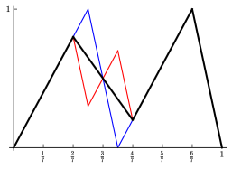
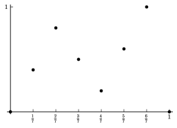
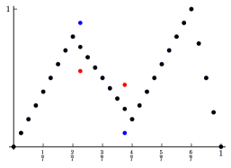
8.3. Restriction and interpolation for $k\geq 2$

Some similar restriction results can be proved for the case of $k$ rows, but this area is much more open. Restrictions seem to require the use of nice polyhedral complexes. The only results known are for the polyhedral complex $\mathcal{P}_{q}$ (Example 3.0) in $\mathbb{R}^{2}$.

Theorem 8.7 ([16, Theorem LABEL:equi3:minimality-check-2d and Theorem LABEL:equi3:theorem:systemNotUnique]).

Let $\pi\colon\mathbb{R}^{2}\to\mathbb{R}$ be a continuous piecewise linear function over $\mathcal{P}_{q}$ and suppose ${\mathchoice{\mbox{\boldmath$\displaystyle\bf f$}}{\mbox{\boldmath$\textstyle\bf f$}}{\mbox{\boldmath$\scriptstyle\bf f$}}{\mbox{\boldmath$\scriptscriptstyle\bf f$}}}\in\tfrac{1}{q}\mathbb{Z}^{2}$. Then the following hold:

1. $\pi$ is minimal for $R_{\mathchoice{\mbox{\boldmath$\displaystyle\bf f$}}{\mbox{\boldmath$\textstyle\bf f$}}{\mbox{\boldmath$\scriptstyle\bf f$}}{\mbox{\boldmath$\scriptscriptstyle\bf f$}}}(\mathbb{R}^{2},\mathbb{Z}^{2})$ if and only if $\pi_{\frac{1}{q}\mathbb{Z}^{2}}$ is minimal for $R_{\mathchoice{\mbox{\boldmath$\displaystyle\bf f$}}{\mbox{\boldmath$\textstyle\bf f$}}{\mbox{\boldmath$\scriptstyle\bf f$}}{\mbox{\boldmath$\scriptscriptstyle\bf f$}}}(\tfrac{1}{q}\mathbb{Z}^{2},\mathbb{Z}^{2})$.

2. If $\pi$ is extreme for $R_{\mathchoice{\mbox{\boldmath$\displaystyle\bf f$}}{\mbox{\boldmath$\textstyle\bf f$}}{\mbox{\boldmath$\scriptstyle\bf f$}}{\mbox{\boldmath$\scriptscriptstyle\bf f$}}}(\mathbb{R}^{2},\mathbb{Z}^{2})$, then $\pi|_{\frac{1}{q}\mathbb{Z}^{2}}$ is extreme for $R_{\mathchoice{\mbox{\boldmath$\displaystyle\bf f$}}{\mbox{\boldmath$\textstyle\bf f$}}{\mbox{\boldmath$\scriptstyle\bf f$}}{\mbox{\boldmath$\scriptscriptstyle\bf f$}}}(\tfrac{1}{q}\mathbb{Z}^{2},\mathbb{Z}^{2})$.

For $k\geq 3$ rows, it is unclear when similar results are possible.

Open question 8.7.

Can Theorem 8.7 be generalized to other triangulations of $\mathbb{R}^{k}$ for $k\geq 2$?

In the special case of diagonally constrained functions in $\mathbb{R}^{2}$, there is a similar result to Theorem 8.6.

Theorem 8.8 ([16, LABEL:equi3:thm:1/4q]).

Let $\pi$ be a minimal continuous piecewise linear function over $\mathcal{P}_{q}$ that is diagonally constrained and ${\mathchoice{\mbox{\boldmath$\displaystyle\bf f$}}{\mbox{\boldmath$\textstyle\bf f$}}{\mbox{\boldmath$\scriptstyle\bf f$}}{\mbox{\boldmath$\scriptscriptstyle\bf f$}}}\in\operatorname{vert}(\mathcal{P}_{q})$. Fix $m\in\mathbb{Z}_{\geq 3}$. Then $\pi$ is extreme for $R_{\mathchoice{\mbox{\boldmath$\displaystyle\bf f$}}{\mbox{\boldmath$\textstyle\bf f$}}{\mbox{\boldmath$\scriptstyle\bf f$}}{\mbox{\boldmath$\scriptscriptstyle\bf f$}}}(\mathbb{R}^{2},\mathbb{Z}^{2})$ if and only if the restriction $\pi\big{|}_{\frac{1}{mq}\mathbb{Z}^{2}}$ is extreme for $R_{\mathchoice{\mbox{\boldmath$\displaystyle\bf f$}}{\mbox{\boldmath$\textstyle\bf f$}}{\mbox{\boldmath$\scriptstyle\bf f$}}{\mbox{\boldmath$\scriptscriptstyle\bf f$}}}(\frac{1}{mq}\mathbb{Z}^{2},\mathbb{Z}^{2})$.

If we know that $\pi$ is diagonally constrained, then this theorem produces an alternative algorithm to Theorem 7.2 to test extremality of $\pi$ by simply restricting to $\tfrac{1}{3q}\mathbb{Z}^{2}$ and testing extremality in the finite dimensional setting. A generalization of this theorem that removes the condition of being diagonally constrained will appear in a forthcoming article [17].

Appendix A Updated compendium of extreme functions

The following tables contain the updated compendium of extreme functions.

Table 1. An updated compendium of known extreme functions for the infinite group problem I. Parametrized classes of continuous functions for the 1-dimensional case with up to two slopes.

Function	Graph		Slopes	Continuity	Notes
gmic			2	C	The famous Gomory mixed integer cut, going back to Gomory’s 1960 paper [32]. Dominates the gomory_fractional cut, which is not minimal (Figure 1).
gj_2_slope			2	C	Two families of continuous extreme functions with 2 slopes, from Gomory–Johnson [39]. By the Gomory–Johnson 2-Slope Theorem (Theorem 2.3), all continuous piecewise linear minimal valid functions with 2 slopes are extreme.
gj_2_slope_repeat			2	C
dg_2_step_mir			2	C	Described by Dash–Günlük [25]. Extremality follows from the 2-Slope Theorem (Theorem 2.3).
kf_n_step_mir			2	C	Described by Kianfar–Fathi [44]. Extremality follows from the 2-Slope Theorem (Theorem 2.3).
bccz_counterexample			1–2	C	Limit of kf_n_step_mir for $n\to\infty$; not a piecewise linear function. Described by Basu–Conforti-Cornuéjols–Zambelli [12]; see § 6.4.

Table 2. An updated compendium of known extreme functions for the infinite group problem II. Parametrized classes of continuous functions for the 1-dimensional case with at least three slopes.

Function	Graph		Slopes	Continuity	Notes
gj_forward_3_slope			3	C	Described by Gomory–Johnson [39].
drlm_backward_3_slope			3	C	Described by Dey–Richard–Li–Miller [28] based on Aráoz–Evans–Gomory–Johnson [4].
dr_projected_sequential_merge_3_slope			3	C	Described by Dey–Richard [27], using their projected_sequential_merge procedure; see Table 5 and § 5.2.
bhk_irrational			3	C	Only extreme when certain parameters are $\mathbb{Q}$-linearly independent. Described by Basu–Hildebrand–Köppe [15]; see § 6.2.
chen_4_slope			4	C	Described by Chen [20].

Table 3. An updated compendium of known extreme functions for the infinite group problem III. Parametrized families of discontinuous functions for the 1-dimensional case.

Function	Graph		Slopes	Continuity	Notes
ll_strong_fractional			1	D	Described by Letchford–Lodi [47]; dominates the gomory_fractional cut (Figure 1). Extreme only if $f\geq\frac{1}{2}$; then special case of dg_2_step_mir_limit, drlm_2_slope_limit (below).
dg_2_step_mir_limit			1	D	Described by Dash–Günlük [25] (“extended 2-step MIR”). Special case of drlm_2_slope_limit (below). Defined as a limit of dg_2_step_mir functions; see § 6 for a discussion of limits.
drlm_2_slope_limit			1	D	From Dey–Richard–Li–Miller [28], generalizing dg_2_step_mir_limit (above). Defined as a limit; see § 6 for a discussion of limits.
drlm_3_slope_limit			2	D	Described by Dey–Richard–Li–Miller [28]. Defined as the limit of drlm_backward_3_slope functions; see § 6 for a discussion of limits.
rlm_dpl1_extreme_3a			2	D	A $\mathrm{DPL}_{1}$-extreme function from Richard–Li–Miller [49, case 3a]. Proved extreme in [45]. (All other $\mathrm{DPL}_{1}$-extreme functions from [49] are known to be special cases of drlm_2_slope_limit and drlm_3_slope_limit.)

Table 4. An updated compendium of known extreme functions for the infinite group problem IV. “Sporadic” functions for the 1-dimensional case. These functions were found by computer experiments. They have not been described in the literature as a member of a parametrized family; but there is no reason to assume this could not be done.

Function	Graph		Slopes	Continuity	Notes
hildebrand_2_sided_discont_1_slope_1			1	D	An extreme function that is discontinuous on both sides of the origin, from Hildebrand (2013, unpublished). Previously unpublished $\clubsuit$
hildebrand_2_sided_discont_2_slope_1			2	D	An extreme function that is discontinuous on both sides of the origin, from Hildebrand (2013, unpublished). Previously unpublished $\clubsuit$
hildebrand_discont_3_slope_1			3	D	A discontinuous extreme function with 3 slopes, from Hildebrand (2013, unpublished). Previously unpublished $\clubsuit$
hildebrand_5_slope_22_1			5	C	An extreme function with 5 slopes, from Hildebrand (2013, unpublished). Several examples are known. Previously unpublished $\clubsuit$
kzh_7_slope_1			7	C	An extreme function with 7 slopes, from Köppe–Zhou [46]. Several examples are known. Previously unpublished $\clubsuit$
kzh_28_slope_1			28	C	An extreme function with 28 slopes, from Köppe–Zhou [46]. The shown graph does not convey the complexity of this function, which has 395 breakpoints in $[0,1]$ sampled from $\frac{1}{778}\mathbb{Z}$. Previously unpublished $\clubsuit$

Table 5. An updated compendium of known extreme functions for the infinite group problem V. Procedures.

	Graphs
Procedure	From	To	Notes
automorphism			From Johnson [43]; see [48, section 19.5.2.1].
multiplicative_homomorphism			See [48, sections 19.4.1, 19.5.2.1].
projected_sequential_merge			Operation $\mathbin{\lozenge_{n}^{1}}$ from Dey–Richard [27]; see § 5.2.
restrict_to_finite_group			Restrictions to finite group problems $R_{f}(\tfrac{1}{q}\mathbb{Z},\mathbb{Z})$ preserve extremality if $f$ and all breakpoints lie in $\tfrac{1}{q}\mathbb{Z}$. See § 8.2.
restrict_to_finite_group(oversampling=3)			If oversampling by a factor $m\geq 3$, the restriction is extreme for $R_{f}(\tfrac{1}{mq}\mathbb{Z},\mathbb{Z})$ if and only if the original function is extreme. See § 8.2.
interpolate_to_infinite_group			Interpolation from finite group problems $R_{f}(\tfrac{1}{q}\mathbb{Z},\mathbb{Z})$ preserves minimality, but in general not extremality. See § 8.2.
two_slope_fill_in			Described by Gomory–Johnson [38], Johnson [43]. For $k=1$, if minimal, equal to interpolate_to_infinite_group (above). For $k>1$, see [48, section 19.5.2.3] and [9, 13] for recent developments.

Table 6. List of notation in the infinite group problem literature

	Gomory–Johnson		Dey et al.		Basu et al.			Surveys
Concept	[37, 38]	[39]	[30, 26]	[28]	[12]	[18]	[15, 16]	[48]	[22]	this
Additive group of reals mod 1	$I$	$G$	$I$	$I$				$I$
Mapping from reals to group elements	$u=\mathcal{F}(x)$		$\mathbb{P}(u)$	$\mathbb{P}(u)$				$u=\mathcal{F}(v)$
Mapping from group elements to canonical reals	$x=|u|$			$\mathbb{P}^{-1}(u)$				$v=\mathcal{F}^{-1}(u)$
Number of rows of the group problem	$1$	$1$	$m$	$m$	$1$	$k$	$k$	$m$	$q$	$k$
Group (domain of solutions, valid functions)	$U=I$	$G$	$I^{m}$	$I^{m}$		$\mathbb{R}^{k}$	$G=\mathbb{R}^{k}$	$G=I^{m}$	$\mathbb{R}^{q}$	$G=\mathbb{R}^{k}$
Subgroup (periodicity)						$\mathbb{Z}^{k}$	$S=\mathbb{Z}^{k}$		$\mathbb{Z}^{q}$	$S=\mathbb{Z}^{k}$
Right-hand side	$u_{0}$	$u_{0}$	$r$	$r$	$f$	$-f$	$\textstyle\bf f$	$r$	$-f$	$\textstyle\bf f$
Group problem	$\mathrm{P}(U,u_{0})$		($m$DIIGP)			(IR)				(6)
Solutions to the group problem	$t(u)$	$\{t(u)\}$	$t(u)$	$t(u)$	$s_{r}$	$s_{r}$	$s(\mathchoice{\mbox{\boldmath$\displaystyle\bf r$}}{\mbox{\boldmath$\textstyle\bf r$}}{\mbox{\boldmath$\scriptstyle\bf r$}}{\mbox{\boldmath$\scriptscriptstyle\bf r$}})$	$t(u)$	$x_{r}$	$y(\mathchoice{\mbox{\boldmath$\displaystyle\bf r$}}{\mbox{\boldmath$\textstyle\bf r$}}{\mbox{\boldmath$\scriptstyle\bf r$}}{\mbox{\boldmath$\scriptscriptstyle\bf r$}})$
Solution set of the group problem	$T(U,u_{0})$		$m$DIIGP	$PI(r,m)$				$\mathrm{MG}(G,\emptyset,r)$	$G_{f}$
Its convex hull							$R_{\mathchoice{\mbox{\boldmath$\displaystyle\bf f$}}{\mbox{\boldmath$\textstyle\bf f$}}{\mbox{\boldmath$\scriptstyle\bf f$}}{\mbox{\boldmath$\scriptscriptstyle\bf f$}}}(G,S)$			$R_{\mathchoice{\mbox{\boldmath$\displaystyle\bf f$}}{\mbox{\boldmath$\textstyle\bf f$}}{\mbox{\boldmath$\scriptstyle\bf f$}}{\mbox{\boldmath$\scriptscriptstyle\bf f$}}}(G,S)$
Its enclosing space							$\mathcal{V}$			$\mathbb{R}^{(G)}$
Valid functions	$\pi(u)$	$\pi(u)$	$\phi(u)$	$\phi(u)$	$\pi(r)$	$\pi(r)$	$\pi(\mathchoice{\mbox{\boldmath$\displaystyle\bf r$}}{\mbox{\boldmath$\textstyle\bf r$}}{\mbox{\boldmath$\scriptstyle\bf r$}}{\mbox{\boldmath$\scriptscriptstyle\bf r$}})$	$\phi(u)$	$\pi(r)$	$\pi(\mathchoice{\mbox{\boldmath$\displaystyle\bf r$}}{\mbox{\boldmath$\textstyle\bf r$}}{\mbox{\boldmath$\scriptstyle\bf r$}}{\mbox{\boldmath$\scriptscriptstyle\bf r$}})$
Set of tight solutions for a valid function		$P(\pi)$	$P(\phi)$		$P(\pi)$	$S(\pi)$				$P(\pi)$
Subadditivity slack	$\nabla(u,v)$						$\Delta\pi(\mathchoice{\mbox{\boldmath$\displaystyle\bf u$}}{\mbox{\boldmath$\textstyle\bf u$}}{\mbox{\boldmath$\scriptstyle\bf u$}}{\mbox{\boldmath$\scriptscriptstyle\bf u$}},\mathchoice{\mbox{\boldmath$\displaystyle\bf v$}}{\mbox{\boldmath$\textstyle\bf v$}}{\mbox{\boldmath$\scriptstyle\bf v$}}{\mbox{\boldmath$\scriptscriptstyle\bf v$}})$			$\Delta\pi(\mathchoice{\mbox{\boldmath$\displaystyle\bf u$}}{\mbox{\boldmath$\textstyle\bf u$}}{\mbox{\boldmath$\scriptstyle\bf u$}}{\mbox{\boldmath$\scriptscriptstyle\bf u$}},\mathchoice{\mbox{\boldmath$\displaystyle\bf v$}}{\mbox{\boldmath$\textstyle\bf v$}}{\mbox{\boldmath$\scriptstyle\bf v$}}{\mbox{\boldmath$\scriptscriptstyle\bf v$}})$
Additivity domain (equality set)		$E(\pi)$	$E(\phi)$		$E(\pi)$	$E(\pi)$	$E(\pi)$			$E(\pi)$

Appendix B List of notation in the literature

Table 6 (on page 6) compares the notation in the present survey with that in selected original articles on the infinite group problem and the surveys [48, 22].

References

- [1] J. Aczél and J. G. Dhombres, Functional equations in several variables, no. 31, Cambridge University Press, 1989.
- [2] C. Aliprantis and K. Border, Infinite dimensional analysis: A hitchhiker’s guide, second ed., Springer Verlag, 2006.
- [3] K. Andersen, Q. Louveaux, R. Weismantel, and L. Wolsey, Inequalities from two rows of a simplex tableau, Integer Programming and Combinatorial Optimization. 12th International IPCO Conference, Ithaca, NY, USA, June 25–27, 2007. Proceedings (M. Fischetti and D. Williamson, eds.), Lecture Notes in Computer Science, vol. 4513, Springer Berlin / Heidelberg, 2007, pp. 1–15, doi:10.1007/978-3-540-72792-7_1.
- [4] J. Aráoz, L. Evans, R. E. Gomory, and E. L. Johnson, Cyclic group and knapsack facets, Mathematical Programming, Series B 96 (2003), 377–408.
- [5] G. Averkov and A. Basu, On the unique-lifting property, Integer Programming and Combinatorial Optimization, Springer, 2014, pp. 76–87.
- [6] E. Balas, Intersection cuts – a new type of cutting planes for integer programming, Operations Research 19 (1971), 19–39.
- [7] E. Balas, S. Ceria, G. Cornuéjols, and N. R. Natraj, Gomory cuts revisited, Operations Research Letters 19 (1996), no. 1, 1–9, MR 97d:90059.
- [8] E. Balas and R. G. Jeroslow, Strengthening cuts for mixed integer programs, European Journal of Operational Research 4 (1980), no. 4, 224–234, doi:10.1016/0377-2217(80)90106-X.
- [9] A. Basu, M. Campêlo, M. Conforti, G. Cornuéjols, and G. Zambelli, Unique lifting of integer variables in minimal inequalities, Mathematical Programming 141 (2013), no. 1–2, 561–576.
- [10] A. Basu, M. Conforti, G. Cornuéjols, and G. Zambelli, Maximal lattice-free convex sets in linear subspaces, Mathematics of Operations Research 35 (2010), 704–720.
- [11] by same author, Minimal inequalities for an infinite relaxation of integer programs, SIAM J. Discret. Math. 24 (2010), 158–168, doi:10.1137/090756375.
- [12] by same author, A counterexample to a conjecture of Gomory and Johnson, Mathematical Programming Ser. A 133 (2012), no. 1–2, 25–38, doi:10.1007/s10107-010-0407-1.
- [13] A. Basu, G. Cornuéjols, and M. Köppe, Unique minimal liftings for simplicial polytopes, Mathematics of Operations Research 37 (2012), no. 2, 346–355, doi:10.1287/moor.1110.0536.
- [14] A. Basu, R. Hildebrand, and M. Köppe, Equivariant perturbation in Gomory and Johnson’s infinite group problem. II. The unimodular two-dimensional case, Integer Programming and Combinatorial Optimization (M. Goemans and J. Correa, eds.), Lecture Notes in Computer Science, vol. 7801, Springer, 2013, pp. 62–73, doi:10.1007/978-3-642-36694-9_6, ISBN 978-3-642-36693-2.
- [15] by same author, Equivariant perturbation in Gomory and Johnson’s infinite group problem. I. The one-dimensional case, Mathematics of Operations Research (2014), doi:10.1287/moor.2014.0660.
- [16] by same author, Equivariant perturbation in Gomory and Johnson’s infinite group problem. III. Foundations for the -dimensional case and applications to , eprint arXiv:1403.4628 [math.OC], 2014.
- [17] by same author, Equivariant perturbation in Gomory and Johnson’s infinite group problem. IV. The general unimodular two-dimensional case, Manuscript, 2014.
- [18] A. Basu, R. Hildebrand, M. Köppe, and M. Molinaro, A -slope theorem for the -dimensional infinite group relaxation, SIAM Journal on Optimization 23 (2013), no. 2, 1021–1040, doi:10.1137/110848608.
- [19] V. Borozan and G. Cornuéjols, Minimal valid inequalities for integer constraints, Mathematics of Operations Research 34 (2009), 538–546, doi:10.1287/moor.1080.0370.
- [20] K. Chen, Topics in group methods for integer programming, Ph.D. thesis, Georgia Institute of Technology, June 2011.
- [21] M. Conforti, G. Cornuéjols, A. Daniilidis, C. Lemaréchal, and J. Malick, Cut-generating functions, Integer Programming and Combinatorial Optimization, Springer, 2013, pp. 123–132.
- [22] M. Conforti, G. Cornuéjols, and G. Zambelli, Corner polyhedra and intersection cuts, Surveys in Operations Research and Management Science 16 (2011), no. 2, 105–120, doi:10.1016/j.sorms.2011.03.001.
- [23] by same author, A geometric perspective on lifting, Operations Research 59 (2011), no. 3, 569–577, doi:10.1287/opre.1110.0916.
- [24] G. Cornuéjols and M. Molinaro, A 3-Slope Theorem for the infinite relaxation in the plane, Mathematical Programming 142 (2013), no. 1–2, 83–105, doi:10.1007/s10107-012-0562-7.
- [25] S. Dash and O. Günlük, Valid inequalities based on simple mixed-integer sets, Mathematical Programming 105 (2006), 29–53, doi:10.1007/s10107-005-0599-y.
- [26] S. S. Dey and J.-P. P. Richard, Facets of two-dimensional infinite group problems, Mathematics of Operations Research 33 (2008), no. 1, 140–166, doi:10.1287/moor.1070.0283.
- [27] by same author, Relations between facets of low- and high-dimensional group problems, Mathematical Programming 123 (2010), no. 2, 285–313, doi:10.1007/s10107-009-0303-8.
- [28] S. S. Dey, J.-P. P. Richard, Y. Li, and L. A. Miller, On the extreme inequalities of infinite group problems, Mathematical Programming 121 (2010), no. 1, 145–170, doi:10.1007/s10107-008-0229-6.
- [29] S. S. Dey and L. A. Wolsey, Constrained infinite group relaxations of MIPs, SIAM Journal on Optimization 20 (2010), no. 6, 2890–2912.
- [30] by same author, Two row mixed-integer cuts via lifting, Mathematical Programming 124 (2010), 143–174.
- [31] R. E. Gomory, Outline of an algorithm for integer solutions to linear programs, Bull. Amer. Math. Soc. 64 (1958), 275–278.
- [32] R. E. Gomory, An algorithm for the Mixed Integer Problem, Tech. Report RM-2597-PR, The RAND Corporation, Santa Monica, CA, 1960.
- [33] R. E. Gomory, An algorithm for integer solutions to linear programs, Recent advances in mathematical programming 64 (1963), 260–302.
- [34] by same author, On the relation between integer and noninteger solutions to linear programs, Proceedings of the National Academy of Sciences of the United States of America 53 (1965), no. 2, 260.
- [35] R. E. Gomory, Some polyhedra related to combinatorial problems, Linear Algebra and its Applications 2(4) (1969), 451–558.
- [36] R. E. Gomory, The atoms of integer programming, Annals of Operations Research 149 (2007), no. 1, 99–102.
- [37] R. E. Gomory and E. L. Johnson, Some continuous functions related to corner polyhedra, I, Mathematical Programming 3 (1972), 23–85, doi:10.1007/BF01585008.
- [38] by same author, Some continuous functions related to corner polyhedra, II, Mathematical Programming 3 (1972), 359–389, doi:10.1007/BF01585008.
- [39] by same author, T-space and cutting planes, Mathematical Programming 96 (2003), 341–375, doi:10.1007/s10107-003-0389-3.
- [40] R. E. Gomory, E. L. Johnson, and L. Evans, Corner polyhedra and their connection with cutting planes, Mathematical Programming 96 (2003), no. 2, 321–339.
- [41] C. Y. Hong, M. Köppe, and Y. Zhou, Sage program for computation and experimentation with the -dimensional Gomory–Johnson infinite group problem, 2014, available from https://github.com/mkoeppe/infinite-group-relaxation-code.
- [42] J. K. Hunter and B. Nachtergaele, Applied analysis, World Scientific, 2001, ISBN 978-9-812-70543-3.
- [43] E. L. Johnson, On the group problem for mixed integer programming, Mathematical Programming Study 2 (1974), 137–179.
- [44] K. Kianfar and Y. Fathi, Generalized mixed integer rounding inequalities: facets for infinite group polyhedra, Mathematical Programming 120 (2009), 313–346.
- [45] M. Köppe and Y. Zhou, An electronic compendium of extreme functions for the Gomory–Johnson infinite group problem, eprint arXiv:1411.5121 [math.OC], 2014.
- [46] by same author, New computer-based search strategies for extreme functions of the Gomory–Johnson infinite group problem, Manuscript, 2015.
- [47] A. N. Letchford and A. Lodi, Strengthening Chvátal–Gomory cuts and Gomory fractional cuts, Operations Research Letters 30 (2002), no. 2, 74–82, doi:10.1016/S0167-6377(02)00112-8.
- [48] J.-P. P. Richard and S. S. Dey, The group-theoretic approach in mixed integer programming, 50 Years of Integer Programming 1958–2008 (M. Jünger, T. M. Liebling, D. Naddef, G. L. Nemhauser, W. R. Pulleyblank, G. Reinelt, G. Rinaldi, and L. A. Wolsey, eds.), Springer Berlin Heidelberg, 2010, pp. 727–801, doi:10.1007/978-3-540-68279-0_19, ISBN 978-3-540-68274-5.
- [49] J.-P. P. Richard, Y. Li, and L. A. Miller, Valid inequalities for MIPs and group polyhedra from approximate liftings, Mathematical Programming 118 (2009), no. 2, 253–277, doi:10.1007/s10107-007-0190-9.
- [50] W. A. Stein et al., Sage Mathematics Software (Version 6.4), The Sage Development Team, 2014, http://www.sagemath.org.
- [51] Y. Zhou, Electronic compendium of extreme functions for the -row Gomory–Johnson infinite group problem, 2014, available from https://github.com/mkoeppe/infinite-group-relaxation-code/.