An ensemble-based system for automatic screening of diabetic retinopathy

Abstract

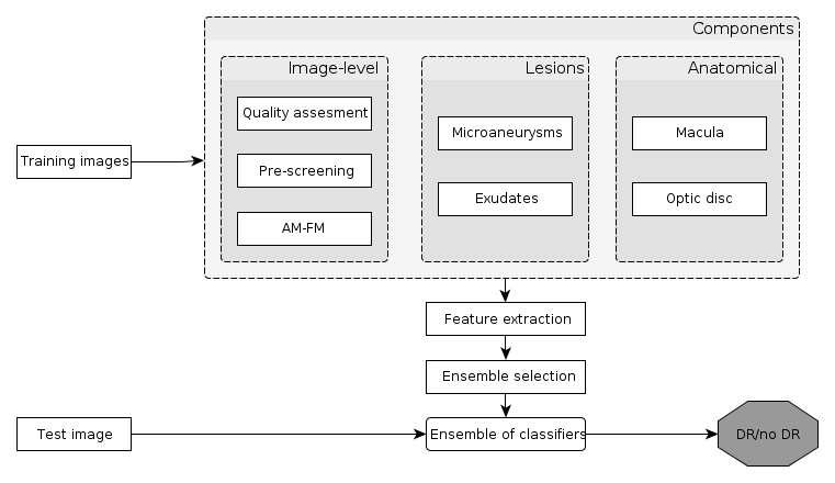
In this paper, an ensemble-based method for the screening of diabetic retinopathy (DR) is proposed. This approach is based on features extracted from the output of several retinal image processing algorithms, such as image-level (quality assessment, pre-screening, AM/FM), lesion-specific (microaneurysms, exudates) and anatomical (macula, optic disc) components. The actual decision about the presence of the disease is then made by an ensemble of machine learning classifiers. We have tested our approach on the publicly available Messidor database, where 90% sensitivity, 91% specificity and 90% accuracy and 0.989 AUC are achieved in a disease/no-disease setting. These results are highly competitive in this field and suggest that retinal image processing is a valid approach for automatic DR screening.

1 Introduction

Diabetic retinopathy (DR) is a consequence of diabetes mellitus which manifests itself in the retina. This disease is one of the most frequent causes of visual impairment in developed countries and is the leading cause of new cases of blindness in the working age population. In 2011, 366 million people were diagnosed with diabetes and a further 280 million people were having risk to develop it. At any point in time, approximately 40% of diabetic patients suffer from DR, out of which an estimated 5% face the sight-threatening form of this disease. Altogether, nearly 75 people go blind every day as a consequence of DR even though treatment is available.

Automatic computer-aided screening of DR is a highly investigated field (Abramoff et al., 2008). The motivation for creating reliable automatic DR screening systems is to reduce the manual effort of mass screening (Fleming et al., 2011), which also raises a financial issue (Scotland et al., 2010). While several studies focus on the recognition of patients having DR (Fleming et al., 2011) (Abramoff et al., 2010b) and considering the specificity of the screening as a matter of efficiency, we show how both sensitivity and specificity can be kept at high level by combining novel screening features and a decision-making process. Especially, our results are very close to meet the recommendations of the British Diabetic Association (BDA) (80% sensitivity and 95% specificity (bda, 1997)).

The basis for an automatic screening system is the analysis of color fundus images (Abramoff et al., 2010a). The key to the early recognition of DR is the reliable detection of microaneurysms (MAs) on the retina, which serves as an essential part for most automatic DR screening systems (Abramoff et al., 2010b) (Jelinek et al., 2006) (Antal and Hajdu, 2012a) (Niemeijer et al., 2009). The role of bright lesions for DR grading has also been investigated with positive (Fleming et al., 2010b) and negative outcomes (Abramoff et al., 2010b) reported. Besides lesions, image quality assesment (Philip et al., 2007) (Fleming et al., 2010a) is also considered to exclude ungradeable images. As a new direction, in (Agurto et al., 2011) an image-level DR recognition algorithm is also presented.

The proposed framework extends the state-of-the-art components of an automatic DR screening system by adding pre-screening (Antal et al., 2012a) and the distance of the macula center (MC) and the optic disc center (ODC) as novel components. We also use image quality assessment as a feature for classification rather than a tool for excluding images. The comparison of the components used in some recently published automatic DR screening systems can be found in Table 1.

Table 1: Comparison of components of the automatic screening system.

Screening system	Image quality	Red lesion	Bright lesion	AM/FM	Pre-screening	MC-ODC
(Abramoff et al., 2010b)		X
(Jelinek et al., 2006)		X
(Antal and Hajdu, 2012a)		X
(Philip et al., 2007)	X	X
(Fleming et al., 2010a)	X	X	X
(Agurto et al., 2011)				X
Proposed	X	X	X	X	X	X

Regarding decision making, automatic DR screening systems either partially follow clinical protocols (e.g. MAs indicate presence of DR) (Jelinek et al., 2006) (Antal and Hajdu, 2012a) (Philip et al., 2007) (Fleming et al., 2010a) or use a machine learning classifier (Abramoff et al., 2008) (Fleming et al., 2010b) (Agurto et al., 2011). A common way to improve reliability in machine learning based applications is to use ensemble-based approaches (Kuncheva, 2004). For medical decision support, ensemble methods have been successfully applied to several fields. In (West et al., 2005) the authors have investigatedthe applicability of ensembles for breast cancer data classification. The prediction of response to certain therapy is improved by the use of a classifier ensemble (Moon et al., 2007). In (Eom et al., 2008) the authors used an ensemble of four classifiers for cardiovascular disease prediction. Ensemble methods are also provided improvement over single classifiers in a natural language processing environment (Doan et al., 2012).

Ensemble systems combine the output of multiple learners with a specific fusion strategy. In (Abramoff et al., 2010b) and (Antal and Hajdu, 2012a), the fusion of multiple MA detectors has proven to be more efficient than a single algorithm for DR classification. The proposed system is ensemble-based at more levels: we consider ensemble systems both in image processing tasks and decision making.

In this paper, a framework for the automatic grading of color fundus images regarding DR is proposed. The approach classifies images based on characteristic features extracted by lesion detection and anatomical part recognition algorithms. These features are then classified using an ensemble of classifiers. As the results show, the proposed approach is highly efficient for this task. The flow chart of our decision making protocol can be seen in Figure 1, as well.

Figure 1: Flow chart of the proposed decision support framework.

We have tested our approach on the publicly available dataset Messidor (see http://messidor.crihan.fr), where it has provided a 0.989 area under the ROC curve (AUC) value in a disease/no disease setting, which is a relatively high figure compared with other state-of-the-art techniques.

The rest of the paper is organized as follows: in section 2, we present the image processing components of our system. Section 3 presents the details of the presented ensemble learning framework. Our experimental methodology and results can be found in sections 4 and 5, respectively. Finally, we draw conclusions in section 6.

2 Components of an automatic system for diabetic retinopathy screening

In this section, the components we used for feature extraction are described. They can be classified as image-level, lesion-specific, and anatomical ones.

2.1 Image-level components

2.1.1 Quality assessment

We classify the images whether they have sufficient quality for a reliable decision with a supervised classifier, where the box count values of the detected vessel system serve as features (Antal and Hajdu, 2009). For vessel segmentation we use an approach proposed in (Kovács and Hajdu, 2011) based on Hidden Markov Random Fields (HMRF). Here, the authors extend the optimization problem of HMRF models considering the tangent vector field of the image to enhance the connectivity of the vascular system consisting of elongated structures.

2.1.2 Pre-screening

During pre-screening (Antal et al., 2012a), we classify the images as severely diseased (abnormal) ones or to be forwarded for further processing. Each image is split into disjoint regions and a simple texture descriptor (inhomogeneity measure) is extracted for each region. Then, a machine learning classifier is trained to classify the images based on these features.

2.1.3 Multi-scale AM/FM based feature extraction

The Amplitude-Modulation Frequency-Modulation (AM/FM) (Agurto et al., 2010) method extracts information from an image, decomposing the green channels of the images into different representations which reflect the intensity, geometry, and texture of the structures with signal processing techniques. The extracted information are then filtered to establish 39 different representations of the image. The images are classified using these features with a supervised learning method. More on this approach can be found in (Agurto et al., 2010).

2.2 Lesion-specific components

2.2.1 Microaneurysm detection

Microaneurysms are normally the earliest signs of DR. They appear as small red dots in the image and their resemblance to vessel fragments make it hard to detect them efficiently. In the proposed system, we apply the MA detection method described in (Antal and Hajdu, 2012a), which is an efficient approach based on $\langle$preprocessing method, candidate extractor$\rangle$ ensembles.

2.2.2 Exudate detection

Exudates are primary signs of diabetic retinopathy and occur when lipid or fat leak from blood vessels or aneurysms. Exudates are bright, small spots, which can have irregular shape. Since exudate detection is also a challenging task, we follow the same complex methodology as for MA detection (Antal and Hajdu, 2012b). Thus, we combine preprocessing methods and candidate extractors in the case of exudate detection, as well (Nagy et al., 2011).

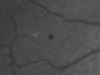
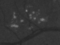
In Figure 2, we show some examples for the appearance of DR-related symptoms in retinal images.

(a) Microaneurysm

(b) Exudates

(c) Inhomogeneity

Figure 2: Some representative visual features to be extracted from the images.

2.3 Anatomical components

2.3.1 Macula detection

The macula is the central region of sharp vision in the human eye with its center referred to as the fovea. Any lesions appearing within the macula can lead to severe loss of vision. Therefore, the efficient detection of the macula is essential in an automatic screening system for DR. The macula is located roughly in the center of the retina, temporal to the optic nerve. In our system, we use the method described in (Antal and Hajdu, 2011), which extracts the largest component from the image which is darker than its surroundings. The location of the macula together with the optic disc described below define some features incorporated in our decision framework.

2.3.2 Optic disc detection

The optic disc is a circular shaped anatomical structure with a bright appearance. It is the area, where the optic nerve enters the eye. If the center and the radius of the optic disc are detected correctly, they can be used as reference data for locating other anatomical parts e.g. the macula. In our system, we use the ensemble-based system described in (Qureshi et al., 2012). Recognizing these anatomical parts is important from two aspects: the appearance of certain lesions at specific positions can indicate a more advanced stage of DR and the presence of rare, but serious defects (like retinal detachment) can ruin the detection of the optic disc and macula.

3 Ensemble learning

The most important expectation for a computer-aided medical system is its high reliability. To ensure that, we use ensemble-based decision making (Kuncheva, 2004). Thus, we have trained several classifiers to separate DR and non-DR cases and fused their results. In this section, we describe how we select the ensemble for DR classification based on the features extracted from the output of the detectors presented in section 2.

3.1 Concepts of ensemble learning

The basic concepts of ensemble learning are presented by following the classic literature (Kuncheva, 2004). These concepts formalize our ensemble-based system for DR grading described in the forthcoming sections.

Definition 1

Let $\Omega=\left\{\omega_{1},\omega_{2},\dots,\omega_{M}\right\}$ be a set of class labels. Then, a function $D:\mathbb{R}^{n}\rightarrow\Omega$ is called a classifier, while a vector $\vec{\chi}=\left(\chi_{1},\chi_{2},\dots,\chi_{n}\right)\in\mathbb{R}^{n}$ is called a feature vector.

Definition 2

Let $h_{1},h_{2},\dots,h_{M}$, $h_{i}:\mathbb{R}^{n}\rightarrow\mathbb{R}$, $i=1,\,\dots,\,M$ be so-called discriminator functions corresponding to the class labels $\omega_{1},\omega_{2},\dots,\omega_{M}$, respectively. Then, the classifier $D$ belonging to these discriminator functions is defined by:

$$D\left(\vec{\chi}\right)=\omega_{j*}\iff h_{j*}\left(\vec{\chi}\right)=\max_{j=1}^{M}\left(h_{j}\left(\vec{\chi}\right)\right).$$ (1)

for all $\vec{\chi}\in\mathbb{R}^{n}$.

Definition 3

Let $D_{1},D_{2},\dots,D_{L}$ be classifiers. Then, the majority voting ensemble classifier ${\cal D}_{maj}:\mathbb{R}^{n}\rightarrow\Omega$ formed from these classifiers is defined as:

$${\cal D}_{maj}\left(\vec{\chi}\right)=\omega_{{i^{*}}}\iff\left|\left\{j:D_{j}\left(\vec{\chi}\right)=\omega_{{i^{*}}},j=1,\dots,M\right\}\right|=\max_{i=1}^{M}\left|\left\{j:D_{j}\left(\vec{\chi}\right)=\omega_{i},j=1,\dots,M\right\}\right|.$$ (2)

Definition 4

Let $D_{1},D_{2},\dots,D_{L}$ be classifiers and $\vec{\beta}=\left(\beta_{1},\beta_{2},\dots,\beta_{L}\right)\in\mathbb{R}^{L}$ be a weight vector assigned to the classifiers. Then, the weighted majority voting ensemble classifier ${\cal D}_{wmaj}:\mathbb{R}^{n}\rightarrow\Omega$ is defined as follows:

$${\cal D}_{wmaj}\left(\vec{\chi}\right)=\omega_{{i^{*}}}\iff\sum_{\begin{subarray}{c}j=1\\ D_{j}\left(\vec{\chi}\right)=\omega_{{i^{*}}}\end{subarray}}^{L}\beta_{j}=\max_{i=1}^{M}\left(\sum_{\begin{subarray}{c}j=1\\ D_{j}\left(\vec{\chi}\right)=\omega_{i}\end{subarray}}^{L}\beta_{j}\right).$$ (3)

Definition 5

Let $D_{1},D_{2},\dots,D_{L}$ be classifiers and $h_{j,i}$ be a discriminator function of the classifier $D_{j}$ for the class $i$, $i=1,\dots,M,\,j=1,\dots,L$. Then, the following algebraic ensemble classifiers can be defined:

$${\cal D}_{avg}\left(\vec{\chi}\right) =\omega_{{i^{*}}}\iff\dfrac{1}{L}\sum_{j=1}^{L}\left(h_{j,{i^{*}}}\left(\vec{\chi}\right)\right)=\max_{i=1}^{M}\left(\dfrac{1}{L}\sum_{j=1}^{L}\left(h_{j,i}\left(\vec{\chi}\right)\right)\right),$$ (4)

$${\cal D}_{pro}\left(\vec{\chi}\right) =\omega_{{i^{*}}}\iff\prod_{j=1}^{L}\left(h_{j,{i^{*}}}\left(\vec{\chi}\right)\right)=\max_{i=1}^{M}\left(\prod_{j=1}^{L}\left(h_{j,i}\left(\vec{\chi}\right)\right)\right),$$ (5)

$${\cal D}_{min}\left(\vec{\chi}\right) =\omega_{{i^{*}}}\iff\min_{j=1}^{L}\left(h_{j,{i^{*}}}\left(\vec{\chi}\right)\right)=\max_{i=1}^{M}\left(\min_{j=1}^{L}\left(h_{j,i}\left(\vec{\chi}\right)\right)\right),$$ (6)

$${\cal D}_{max}\left(\vec{\chi}\right) =\omega_{{i^{*}}}\iff\max_{j=1}^{L}\left(h_{j,{i^{*}}}\left(\vec{\chi}\right)\right)=\max_{i=1}^{M}\left(\max_{j=1}^{L}\left(h_{j,i}\left(\vec{\chi}\right)\right)\right).$$ (7)

3.2 Ensemble selection

To select the optimal ensemble for DR classification, we have trained several well-known classifiers that will be described in section 4.3. Each ensemble is a subset of these classifiers. Several approaches have been tested for selecting the best subset of classifiers ${\cal D}$ for DR grading. The following search methods were investigated based on (Ruta and Gabrys, 2005) for a fixed set of classifiers $\{D_{1},\,\dots,\,D_{L}\}$ and energy function $E:{\cal D}\subseteq\{D_{1},\,\dots,\,D_{L}\}\to{\mathbb{R}}_{\geq 0}$:

• Forward search: First, the best individual classifier is selected. Then, further classifiers are added if the performance of the ensemble increases. The process ends when no further increase of performance is reached by adding more classifiers. Algorithm 1 gives a formal description of this search method.

  Algorithm 1 Forward search

  1.  ${\cal D}\leftarrow\operatornamewithlimits{argmax}\left(E\left(\{D_{1}\}\right),E\left(\{D_{2}\}\right),\dots,E\left(\{D_{L}\}\right)\right)$

  2.  $e_{best}\leftarrow E\left({\cal D}\right)$

  3.  for all $D_{i}\notin{\cal D},i=1\,\dots\,L$ do

  4.     $e\leftarrow E\left({\cal D}\cup\{D_{i}\}\right)$

  5.     if $e>e_{best}$ then

  6.        ${\cal D}\leftarrow{\cal D}\cup\{D_{i}\}$

  7.        $e_{best}\leftarrow e$

  8.     end if

  9.  end for

  10.  return  ${\cal D}$

• Backward search: First, all classifiers are considered as members of the ensemble. Then, classifiers are removed from the ensemble while the performance of the ensemble increases. See Algorithm 2 for a formal description.

  Algorithm 2 Backward search

  1.  ${\cal D}\leftarrow\{D_{1},\,\dots,\,D_{L}\}$

  2.  $e_{best}\leftarrow E\left({\cal D}\right)$

  3.  for all $D_{i}\in{\cal D}$ do

  4.     $e\leftarrow E\left({\cal D}\setminus\{D_{i}\}\right)$

  5.     if $e>e_{best}$ then

  6.        ${\cal D}\leftarrow{\cal D}\setminus\{D_{i}\}$

  7.        $e_{best}\leftarrow e$

  8.     end if

  9.  end for

  10.  return  ${\cal D}$

For comparison, we also consider the following two ensembles besides the ones found by the search methods:

• All: All classifiers are members of the ensemble.

• Single best: The ensemble contains only the best performing classifier.

4 Methodology

4.1 Messidor database

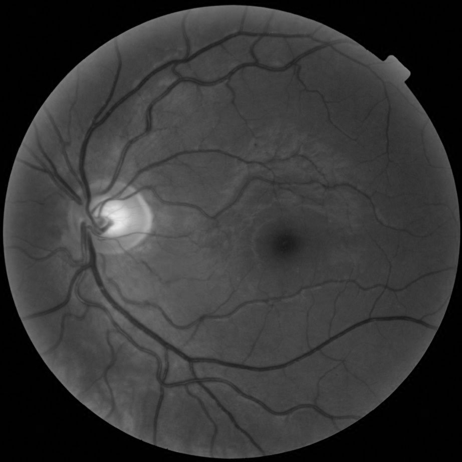
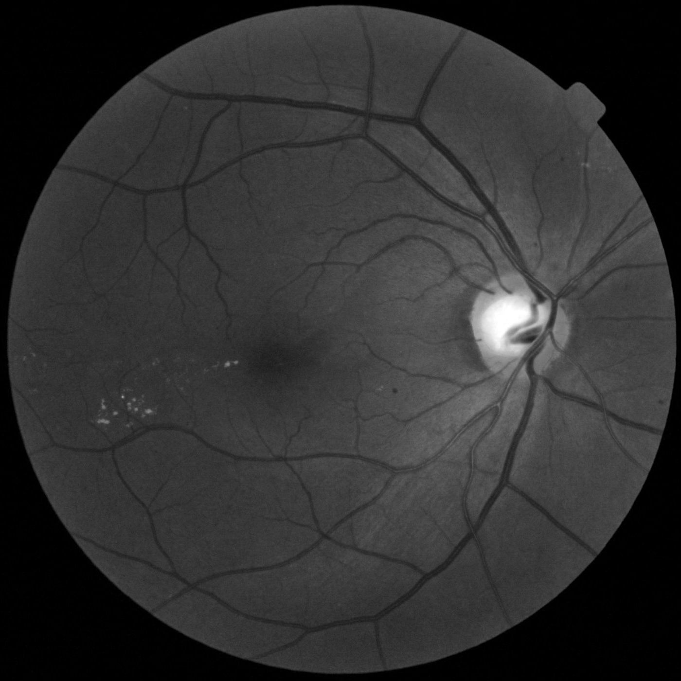
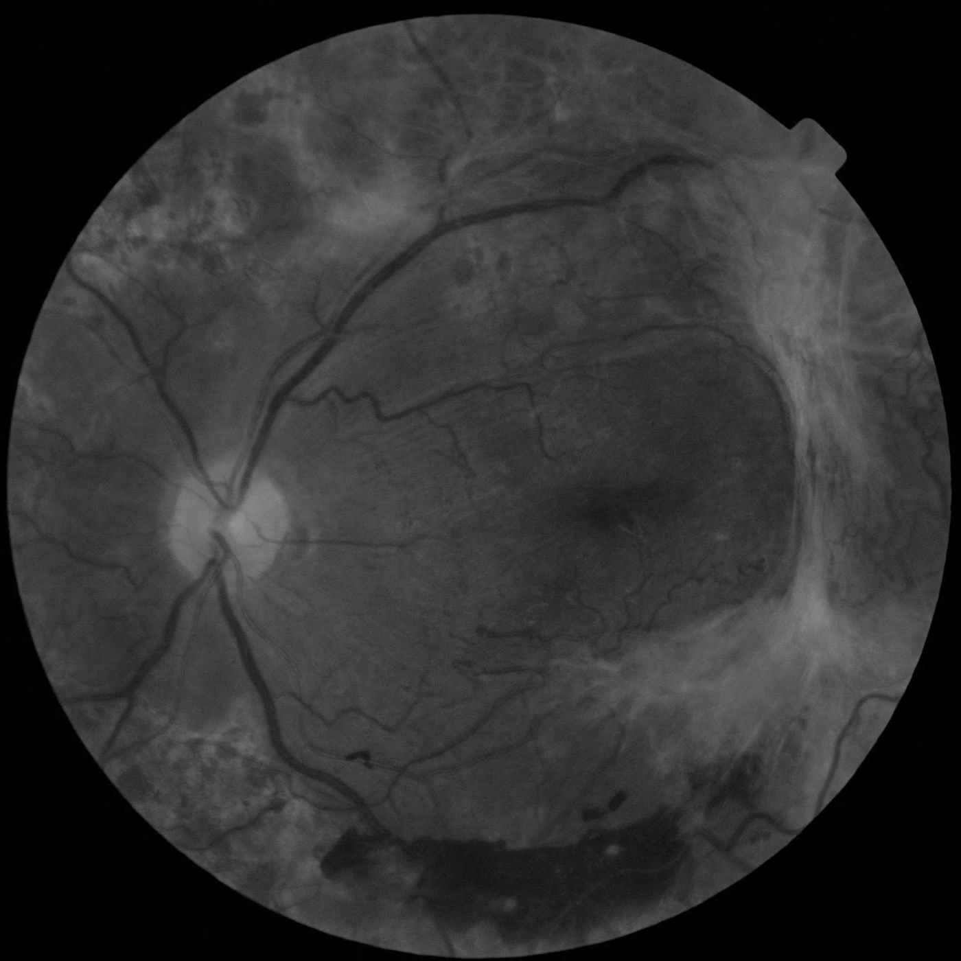
For experimental studies, we consider the publicly available Messidor database that consists of 1200 losslessly compressed images with $45^{\circ}$ FOV and different resolutions ($440\times 960$, $2240\times 1488$ and $2304\times 1536$ pixels). For each image, a grading score ranging from R0 to R3 is also provided. These grades correspond to the following clinical conditions: a patient with grade R0 has no DR. R1 and R2 are mild and severe cases of non-proliferative retinopathy, respectively. Finally, R3 stands for the most serious condition. The grading is based on the appearance of MAs, haemorrhages and neovascularization. The corresponding proportion of the images in the Messidor dataset: 540 R0 (46%), 153 R1 (12.75%), 247 R2 (20.58%) and 260 R3 (21.67%). This database is made available by the Messidor program partners (see http://messidor.crihan.fr). Some example images corresponding to the different grading scores are shown in Figure 3.

(a) R0

(b) R1

(c) R2

(d) R3

Figure 3: Representative images having different grades (R0, R1, R2, R3) from the Messidor database.

4.2 Features

In this section, we describe the features that were extracted from the output of the image processing algorithms presented in section 2. These features are also summarized in Table 2.

$\bullet~{}\chi_{0}$ is the result of quality assessment, which is a real number between 0 (worst) and 1 (best) quality for a color fundus image.

$\bullet~{}\chi_{1}$ is a binary variable representing the result of pre-screening, where 1 indicates severe retinal abnormality and 0 its lack.

$\bullet~{}$ As an essential part of a DR screening system, features $\chi_{2}-\chi_{7}$ describe the results of MA detection. More precisely, $\chi_{i}$ ($i=2,\dots,7$) stand for the number of MAs found at the confidence levels $\alpha=0.5,\dots,1$, respectively.

$\bullet~{}\chi_{8}-\chi_{16}$ contain the same information as $\chi_{2}-\chi_{7}$ for exudates. However, as exudates are represented by a set of points rather than the number of pixels constructing the lesions, these features are normalized by dividing the number of lesions with the diameter of the ROI to compensate different image sizes.

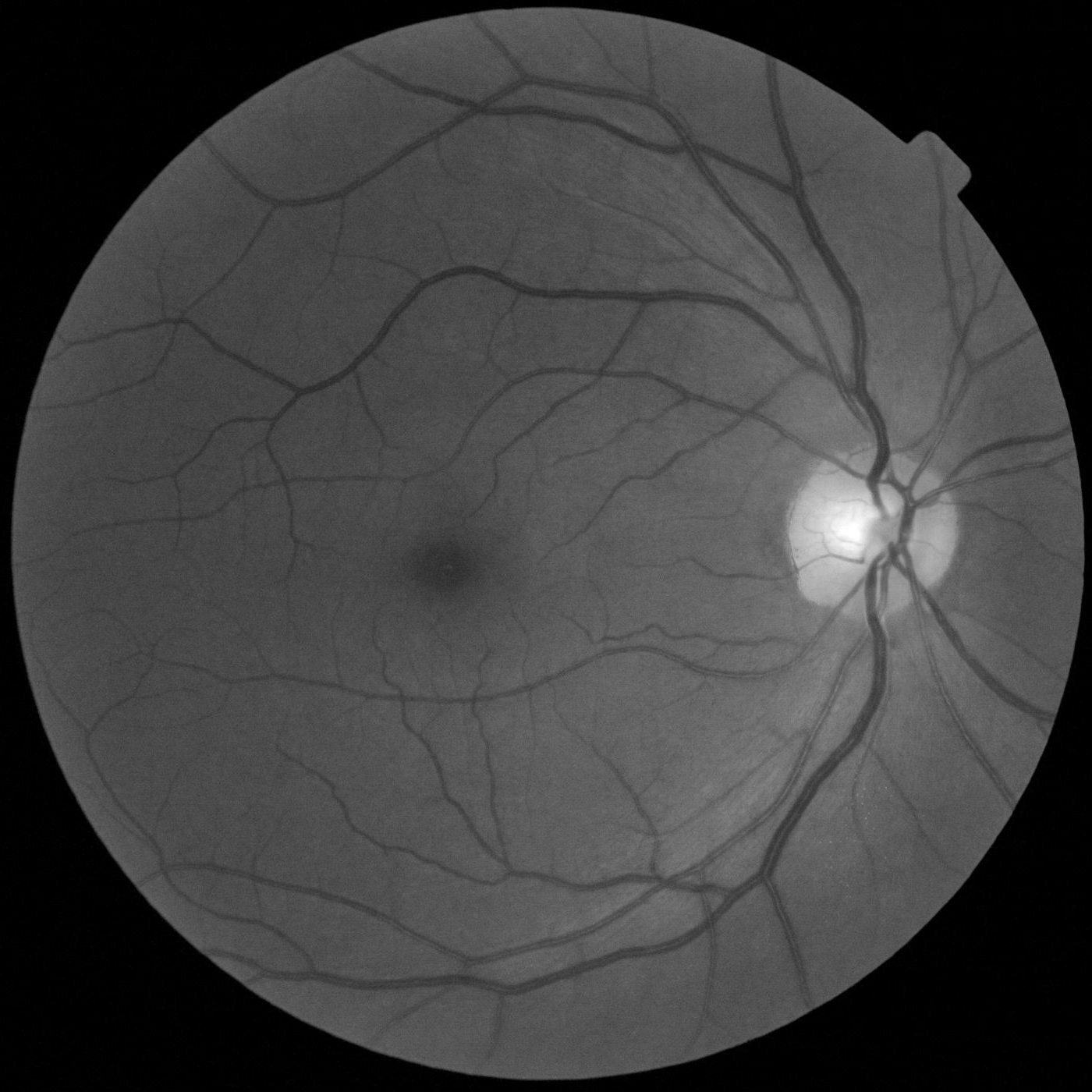
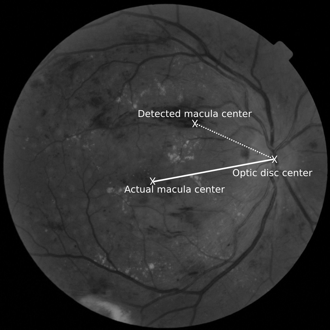
$\bullet~{}$ Since abnormalities can make it harder to detect certain anatomical landmarks in an image, $\chi_{17}$ represents the euclidean distance of the center of the macula and the center of the optic disc to provide important information regarding the patient’s condition (see Figure 4 for an example). This feature is also normalized with the diameter of the ROI.

Figure 4: The difference between the actual and the detected optic disc and macula centers.

$\bullet~{}\chi_{18}$ is the result of the AM/FM-based classification, which is a non-negative scalar indicating the confidence of the detection of DR. The larger $\chi_{18}$, the higher the probability that DR is present.

Table 2: Features for DR grading.

Feature	Description of feature
$\chi_{0}$	The result of quality assessment.
$\chi_{1}$	The result of pre-screening (non-severe DR / severe DR).
$\chi_{2}-\chi_{7}$	The number of MAs detected at confidence levels $\alpha=0.5,\,\dots,\,1.0$, resp.
$\chi_{8}-\chi_{16}$	The number of exudate pixels at confidence levels $\alpha=0.1,\,\dots,\,1.0$, resp.
$\chi_{17}$	The euclidean distance of the center of the macula and the center of the optic disc.
$\chi_{18}$	The result of the AM/FM-based classification (No DR/DR).

4.3 Classifiers and energy functions

We have considered the following classifiers as potential members of ensembles:

• Alternating Decision Tree,

• kNN,

• AdaBoost,

• Multilayer Perceptron,

• Naive Bayes,

• Random Forest,

• SVM,

• Pattern classifier (Antal et al., 2012b).

For ensemble selection, we have considered the following energy functions:

$$\textit{Sensitivity}=\dfrac{TP}{TP+FN},$$ (8)

$$\textit{Accuracy}=\dfrac{TP+TN}{TP+FP+TN+FN},~{}\mbox{and}$$ (9)

$$\textit{F-score}=\dfrac{2TP}{2TP+FN+FP},$$ (10)

where $TP$, $FP$, $TN$, $FN$ represent the true and false positive and true and false negative classifications of the system, respectively. In the rest of the paper, when the functions (8), (9), (10) are set in italic, we refer to them as energy functions; their normal typesetting forms mean the same function, but applied to evaluation purposes.

Note that to fit this realization to the general framework, the above features and classifiers should be considered as the ones $\chi_{1},\dots,\chi_{18}$ and $D_{1},\dots,D_{8}$ given in section 3.1, respectively. Moreover, any of the energy functions (8), (9), (10) should be assigned to $E$ in section 3.2.

4.4 Training and evaluation

10-fold cross-validation have been used for both the training phase and for the evaluation of the ensembles. The figures given in section 5 are the average values of the 10-fold cross-validation for the respective energy functions in each case on the Messidor database. To measure the performance of the ensembles, we disclose the following descriptive values: Sensitivity (8), Accuracy (9), and Specificity with the latter one is defined as:

$$\mbox{Specificity}=\dfrac{TN}{TN+FP}.$$ (11)

To compare our results with other approaches, we have fitted Receiver Operating Characteristic curves to the results and calculated the area under these curves ($AUC$) using JROCFIT (Eng, 2013). We have evaluated the ensemble creation strategies in two scenarios:

• R0 vs R1: First, we have investigated whether the image contains early signs of retinopathy (R1) or not (R0), that is, $\Omega=\{\mbox{R0},\mbox{R1}\}$ in Definition 1. Discriminating these two classes are the most challenging task of DR screening, since R1 usually contain only minor and visually less distinguishable signs of DR than advanced stages (R2, R3).
  

• No DR/DR: Second, we have measured the classification performance of the ensembles between all diseased categories (R1, R2, R3) and the normal one (R0), that is, $\Omega=\{\mbox{R0},\{\mbox{R1}\cup\mbox{R2}\cup\mbox{R3}\}\}$ in Definition 1.

5 Results

5.1 Ensemble selection

Tables 3 and 4 contain the Sensitivity, Specificity and Accuracy values corresponding to the different fusion strategies and search methods for the scenario R0 vs R1, while Tables 5 and 6 relate to the scenario No DR/DR, respectively. For both scenarios, the table entries corresponding to the most accurate ensembles are set in bold. For better comparison, we also disclose the accuracy values for the ensembles containing all classifiers in table 7.

Table 3: DR grading results for scenario R0 vs R1 on the Messidor database with forward search method using different fusion strategies and energy functions. Each cell contains the Sensitivity/Specificity/accuracy of the best ensemble for the corresponding setup.

R0 vs R1 – Forward search
	Sensitivity	Accuracy	F-Score
${\cal D}_{maj}$	98%/82%/83%	77%/90%/88%	75%/89%/86%
${\cal D}_{wmaj}$	76%/90%/88%	83%/88%/87%	87%/87%/87%
${\cal D}_{avg}$	86%/88%/88%	77%/88%/86%	82%/89%/88%
${\cal D}_{pro}$	74%/90%/86%	80%/88%/87%	79%/89%/87%
${\cal D}_{min}$	74%/90%/87%	74%/91%/87%	85%/88%/88%
${\cal D}_{max}$	77%/90%/87%	71%/91%/86%	81%/88%/87%

Table 4: DR grading results for scenario R0 vs R1 on the Messidor database with backward search method using different fusion strategies and energy functions. Each cell contains the Sensitivity/Specificity/accuracy of the best ensemble for the corresponding setup.

R0 vs R1 – Backward search
	Sensitivity	Accuracy	F-Score
${\cal D}_{maj}$	88%/87%/87%	92%/88%/89%	84%/89%/88%
${\cal D}_{wmaj}$	98%/82%/84%	85%/88%/88%	69%/88%/83%
${\cal D}_{avg}$	85%/89%/88%	94%/90%/90%	93%/90%/90%
${\cal D}_{pro}$	0%/78%/78%	0%/79%/80%	0%/78%/80%
${\cal D}_{min}$	81%/90%/88%	83%/89%/88%	64%/96%/85%
${\cal D}_{max}$	98%/81%/82%	98%/81%/83%	76%/89%/86%

Table 5: DR grading results for scenario No DR/DR on the Messidor database with forward search method using different fusion strategies and energy functions. Each cell contains the Sensitivity/Specificity/accuracy of the best ensemble for the corresponding setup.

No DR/DR – Forward search
	Sensitivity	Accuracy	F-Score
${\cal D}_{maj}$	88%/79%/86%	91%/76%/88%	88%/84%/88%
${\cal D}_{wmaj}$	88%/84%/87%	88%/88%/87%	91%/68%/85%
${\cal D}_{avg}$	86%/83%/85%	88%/85%/88%	89%/81%/87%
${\cal D}_{pro}$	95%/38%/60%	85%/83%/85%	89%/72%/85%
${\cal D}_{min}$	80%/95%/80%	88%/82%/87%	87%/78%/86%
${\cal D}_{max}$	92%/50%/72%	90%/76%/87%	88%/76%/86%

Table 6: DR grading results for scenario No DR/DR on the Messidor database with backward search method using different fusion strategies and energy functions. Each cell contains the Sensitivity/Specificity/accuracy of the best ensemble for the corresponding setup.

No DR/DR – Backward search
	Sensitivity	Accuracy	F-Score
${\cal D}_{maj}$	89%/78%/86%	90%/80%/89%	90%/88%/90%
${\cal D}_{wmaj}$	88%/93%/85%	86%/83%/85%	89%/90%/88%
${\cal D}_{avg}$	90%/91%/90%	87%/80%/86%	89%/92%/90%
${\cal D}_{pro}$	97%/56%/80%	88%/85%/88%	90%/73%/86%
${\cal D}_{min}$	81%/97%/82%	81%/97%/82%	81%/98%/83%
${\cal D}_{max}$	93%/68%/86%	93%/77%/89%	89%/83%/88%

Table 7: DR grading results on the Messidor database with all of the classifiers included in the ensemble. Each cell contains the Sensitivity/Specificity/accuracy of the best ensemble for the corresponding setup.

All classifiers
	R0 vs R1	No DR/DR
${\cal D}_{maj}$	96%/84%/85%	88%/79%/86%
${\cal D}_{wmaj}$	85%/87%/87%	88%/84%/87%
${\cal D}_{avg}$	80%/88%/87%	86%/83%/85%
${\cal D}_{pro}$	100%/78%/78%	95%/38%/60%
${\cal D}_{min}$	48%/95%/69%	80%/95%/80%
${\cal D}_{max}$	95%/79%/80%	92%/50%/72%

Regarding the scenario R0 vs R1, from Table 4 we can see that the best performing ensemble achieved 94% Sensitivity, 90% Specificity and 90% Accuracy using backward search, output fusion strategy ${\cal D}_{avg}$ and energy function Accuracy. For the scenario No DR/DR, 90% Sensitivity, 91% Specificity and 90% Accuracy are achieved with the same search method and fusion strategy (see Table 6). However, the energy function in this case is Sensitivity. For a fair comparison, we also disclose the aggregated results for the energy functions and search methods in Tables 8, and 10 for the scenario R0 vs R1, and in Tables 9, and 11 for the scenario No DR/DR, respectively.

5.1.1 Energy functions

For scenario R0 vs R1 we can state that while the energy functions Sensitivity and Accuracy have performed similarly, F-score has provided less accurate ensembles. For scenario No DR/DR all the three energy functions performed similarly. The difference in the effectiveness of the measure F-score probably lies in the fact that the dataset for scenario R0 vs R1 is biased to R0, since it contains much more instances belonging to that class. That is, the energy functions Accuracy and Sensitivity look more robust for less balanced datasets.

Table 8: Comparison of the energy functions for the scenario R0 vs R1.

R0 vs R1
Energy function	Sensitivity	Specificity	Accuracy
Sensitivity	86%	86%	86%
Accuracy	84%	88%	87%
F-score	81%	88%	80%

Table 9: Comparison of the energy functions for the scenario No DR/DR.

No DR/DR
Energy function	Sensitivity	Specificity	Accuracy
Sensitivity	90%	79%	86%
Accuracy	88%	84%	87%
F-score	88%	82%	87%

5.1.2 Search methods

As for the search methods, the accuracy of the forward and backward search method are similar. However, in both scenarios, the Sensitivity and Specificity values are more balanced for the backward strategy, which is desired for a grading system.

Table 10: Comparison of the search methods for the scenario R0 vs R1.

R0 vs R1
Search method	Sensitivity	Specificity	Accuracy
Forward	80%	89%	87%
Backward	88%	86%	86%
All	84%	85%	81%

Table 11: Comparison of the search methods for the scenario No DR/DR.

R0 vs R1
Search method	Sensitivity	Specificity	Accuracy
Forward	90%	78%	87%
Backward	88%	84%	87%
All	88%	71%	79%

5.1.3 Classifier output fusion strategies

In Tables 12, and 13 the comparison of the fusion strategies can be observed. The experimental results indicate that ${\cal D}_{avg}$ is the most effective strategy for both scenarios. The aggregated results confirm this observation. However, ${\cal D}_{maj}$ and ${\cal D}_{wmaj}$ have also provided similar results, suggesting possible alternative choices.

Table 12: Comparison of classifier output fusion strategies for the scenario R0 vs R1.

R0 vs R1
Fusion strategy	Sensitivity	Specificity	Accuracy
${\cal D}_{maj}$	87%	87%	87%
${\cal D}_{wmaj}$	83%	87%	86%
${\cal D}_{avg}$	85%	89%	88%
${\cal D}_{pro}$	33%	82%	82%
${\cal D}_{min}$	73%	92%	85%
${\cal D}_{max}$	85%	86%	84%

Table 13: Comparison of classifier output fusion strategies for the scenario No DR/DR.

No DR/DR
Fusion strategy	Sensitivity	Specificity	Accuracy
${\cal D}_{maj}$	89%	80%	88%
${\cal D}_{wmaj}$	88%	83%	87%
${\cal D}_{avg}$	88%	84%	88%
${\cal D}_{pro}$	91%	69%	81%
${\cal D}_{min}$	84%	89%	84%
${\cal D}_{max}$	91%	77%	85%

To conclude on the analysis of ensemble selection approaches, it can be stated that backward ensemble search method with energy functions Sensitivity or Accuracy and fusion strategy ${\cal D}_{avg}$ can be recommended for ensemble selection for automatic DR screening.

5.2 Comparison with other automatic DR screening systems

It is challenging to compare our approach with other methods. As we can see in Table 14, most research groups not only evaluated their approach on private datasets, but the proportion of images showing signs of DR is also completely different. Moreover, the most meaningful measure, the area under the ROC curves is not always disclosed either. However, the proposed approach has provided significantly better performance then the other state-of-the-art techniques regarding the clinically important measures. Also note that this comparison was able to be made only for the scenario No DR/DR because of the lack of data for scenario R0 vs R1 from the other systems.

Table 14: Comparison of automatic DR screening systems.

System	Cases having DR	Sensitivity	Specificity	AUC
(Abramoff et al., 2008)	4.8%	84%	64%	0.84
(Abramoff et al., 2010b)	4.96%	N/A	N/A	0.86
(Jelinek et al., 2006)	30%	85%	90%	N/A
(Antal and Hajdu, 2012a)	46%	76%	88%	0.90
(Philip et al., 2007)	37.5%	90.5%	54.7%	N/A
(Fleming et al., 2010a)	35.88%	87%	50.4%	N/A
(Agurto et al., 2011)	74.43%	N/A	N/A	0.81
(Agurto et al., 2011)	76.26%	N/A	N/A	0.89
Proposed	46%	90%	91%	0.989

In (Antal and Hajdu, 2012a), we have reported grading results for the dataset Messidor based on only MA detection for both scenarios. The comparative results between the proposed system and (Antal and Hajdu, 2012a) are given in Table 15 for the scenario R0 vs R1, and in Table 16 for the scenario No DR/DR, respectively. To highlight the efficiency of the ensemble-based approach, we have included the results corresponding to a single classifier based decision, as well. As we can see, the proposed system outpeforms both (Antal and Hajdu, 2012a) and the single classifier approach. It is also interesting to note that the single classifier approach clearly performs better than (Antal and Hajdu, 2012a), which is based solely on the detection of MAs. This observation also confirms the necessity of the wide range of components.

Figure 5: ROC curves of automatic DR screening systems evaluated on the Messidor dataset for the scenario R0 vs R1.

Table 15: Comparison of automatic DR screening systems evaluated on the Messidor dataset for the scenario R0 vs R1.

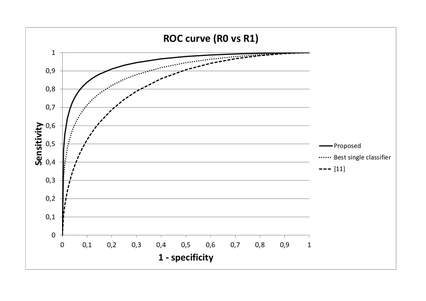
R0 vs R1
System	Sensitivity	Specificity	Accuracy	AUC
(Antal and Hajdu, 2012a)	97%	14%	32%	0.826
Best single classifier	85%	87%	86%	0.893
Proposed	94%	90%	90%	0.942

Figure 6: ROC curves of automatic DR screening systems evaluated on the Messidor dataset for the scenario No DR/DR.

Table 16: Comparison of automatic DR screening systems evaluated on the Messidor dataset for the scenario No DR/DR.

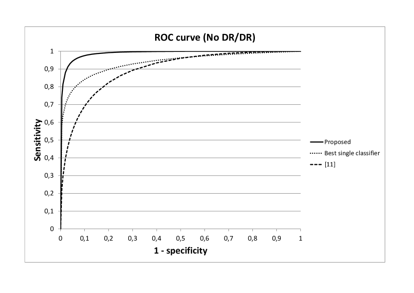
No DR/DR
System	Sensitivity	Specificity	Accuracy	AUC
(Antal and Hajdu, 2012a)	76%	88%	82%	0.90
Best single classifier	90%	81%	86%	0.936
Proposed	90%	91%	90%	0.989

6 Conclusion

In this paper, we have proposed an ensemble-based automatic DR screening system. Opposite to the state-of-the-art methods, we have used image-level, lesion-specific and anatomical components at the same time. To strengthen the reliability of our approach, we have created an ensemble of classifiers. We have discussed extensively on how an efficient ensemble for such a task can be found. Our approach has been validated on the publicly available dataset Messidor, where an outstanding 0.989 area under the ROC curve is achieved. The presented results outperform the current state-of-the-art techniques, which can be reasoned by the well-known observation that ensemble-based systems often lead to higher accuracies. It is also worth noting that our system can be very easily extended by adding more/other components and classifiers. The sensitivity/specificity results (90%/91%) we have achieved are also close to the recommendations of the British Diabetic Association (BDA) (80%/95%) for DR screening (bda, 1997).

References

- bda (1997) , 1997. Retinal photography screening for diabetic eye disease. Tech. rep., British Diabetic Association.
- Abramoff et al. (2010a) Abramoff, M., Garvin, M., Sonka, M., 2010a. Retinal imaging and image analysis. IEEE Reviews in Biomedical Engineering 3, 169 –208.
- Abramoff et al. (2008) Abramoff, M., Niemeijer, M., Suttorp-Schulten, M., Viergever, M. A., Russel, S. R., van Ginneken, B., 2008. Evaluation of a system for automatic detection of diabetic retinopathy from color fundus photographs in a large population of patients with diabetes. Diabetes Care 31, 193–198.
- Abramoff et al. (2010b) Abramoff, M., Reinhardt, J., Russell, S., Folk, J., Mahajan, V., Niemeijer, M., Quellec, G., 2010b. Automated early detection of diabetic retinopathy. Ophthalmology 117 (6), 1147–1154.
- Agurto et al. (2011) Agurto, C., Barriga, E. S., Murray, V., Nemeth, S., Crammer, R., Bauman, W., Zamora, G., Pattichis, M. S., Soliz, P., 2011. Automatic detection of diabetic retinopathy and age-related macular degeneration in digital fundus images. Investigative Ophthalmology & Visual Science 52 (8), 5862–5871.
- Agurto et al. (2010) Agurto, C., Murray, V., Barriga, E., Murillo, S., Pattichis, M., Davis, H., Russell, S., Abramoff, M., Soliz, P., feb. 2010. Multiscale AM-FM methods for diabetic retinopathy lesion detection. IEEE Transactions on Medical Imaging 29 (2), 502 –512.
- Antal and Hajdu (2009) Antal, B., Hajdu, A., 2009. A prefiltering approach for an automatic screening system. In: Proceedings of the IEEE International Symposium on Intelligent Signal Processing. pp. 265–268.
- Antal and Hajdu (2011) Antal, B., Hajdu, A., 2011. A stochastic approach to improve macula detection in retinal images. Acta Cybernetica 20, 5–15.
- Antal and Hajdu (2012a) Antal, B., Hajdu, A., 2012a. An ensemble-based system for microaneurysm detection and diabetic retinopathy grading. IEEE Transactions on Biomedical Engineering 59, 1720 – 1726.
- Antal and Hajdu (2012b) Antal, B., Hajdu, A., 2012b. Improving microaneurysm detection using an optimally selected subset of candidate extractors and preprocessing methods. Pattern Recognition 45 (1), 264 – 270.
- Antal et al. (2012a) Antal, B., Hajdu, A., Szabó-Maros, Z., Török, Z., Csutak, A., Pető, T., 2012a. A two-phase decision support framework for the automatic screening of digital fundus images. Journal of Computational Science 3, 262–268.
- Antal et al. (2012b) Antal, B., Lázár, I., Hajdu, A., 2012b. An Ensemble Approach to Improve Microaneurysm Candidate Extraction. Vol. 222 of Communications in Computer and Information Science. Springer Verlag, Ch. Signal Processing and Multimedia Applications, pp. 378–394.
-
Doan et al. (2012)
Doan, S., Collier, N., Xu, H., Duy, P., Phuong, T., 2012. Recognition of
medication information from discharge summaries using ensembles of
classifiers. BMC Medical Informatics and Decision Making 12 (1), 1–10.
URL http://dx.doi.org/10.1186/1472-6947-12-36 - Eng (2013) Eng, J., 2013. ROC analysis: web-based calculator for ROC curves. http://www.jrocfit.org Downloaded on 07/11/2012.
Eom et al. (2008)
Eom, J.-H., Kim, S.-C., Zhang, B.-T., 2008. Aptacdss-e: A classifier
ensemble-based clinical decision support system for cardiovascular disease
level prediction. Expert Systems with Applications 34 (4), 2465 – 2479.
URL http://www.sciencedirect.com/science/article/pii/S095741740700139X - Fleming et al. (2010a) Fleming, A. D., Goatman, K. A., Philip, S., Prescott, G. J., Sharp, P. F., Olson, J. A., 2010a. Automated grading for diabetic retinopathy: a large-scale audit using arbitration by clinical experts. British Journal of Ophthalmology 94 (12), 1606–1610.
- Fleming et al. (2010b) Fleming, A. D., Goatman, K. A., Philip, S., Williams, G. J., Prescott, G. J., Scotland, G. S., McNamee, P., Leese, G. P., Wykes, W. N., Sharp, P. F., Olson, J. A., , S. D. R. C. R. N., Jun 2010b. The role of haemorrhage and exudate detection in automated grading of diabetic retinopathy. Br J Ophthalmol 94 (6), 706–711.
- Fleming et al. (2011) Fleming, A. D., Philip, S., Goatman, K. A., Prescott, G. J., Sharp, P. F., Olson, J. A., Jul 2011. The evidence for automated grading in diabetic retinopathy screening. Curr Diabetes Rev 7 (4), 246–252.
- Jelinek et al. (2006) Jelinek, H. J., Cree, M. J., Worsley, D., Luckie, A., Nixon, P., 2006. An automated microaneurysm detector as a tool for identification of diabetic retinopathy in rural optometric practice. Clinical and Experimental Optometry 89 (5), 299–305.
- Kovács and Hajdu (2011) Kovács, G., Hajdu, A., 2011. Extraction of vascular system in retina images using averaged one-dependence estimators and orientation estimation in hidden markov random fields. In: Proceedings of the IEEE International Symposium on Biomedical Imaging. pp. 693 –696.
- Kuncheva (2004) Kuncheva, L. I., 2004. Combining Pattern Classifiers. Methods and Algorithms. Wiley.
- Moon et al. (2007) Moon, H., Ahn, H., Kodell, R. L., Baek, S., Lin, C.-J., Chen, J. J., 2007. Ensemble methods for classification of patients for personalized medicine with high-dimensional data. Artificial intelligence in medicine 41, 197–201.
- Nagy et al. (2011) Nagy, B., Harangi, B., Antal, B., Hajdu, A., 2011. Ensemble-based exudate detection in color fundus images. In: Proceedings of the International Symposium on Image and Signal Processing and Analysis. pp. 700–703.
Niemeijer et al. (2009)
Niemeijer, M., Abramoff, M. D., van Ginneken, B., May 2009. Information
fusion for diabetic retinopathy cad in digital color fundus photographs. IEEE
Trans Med Imaging 28 (5), 775–785.
URL http://dx.doi.org/10.1109/TMI.2008.2012029 - Philip et al. (2007) Philip, S., Fleming, A. D., Goatman, K. A., Fonseca, S., Mcnamee, P., Scotland, G. S., Prescott, G. J., Sharp, P. F., Olson, J. A., 2007. The efficacy of automated disease/no disease grading for diabetic retinopathy in a systematic screening programme. British Journal of Ophthalmology 91 (11), 1512–1517.
Qureshi et al. (2012)
Qureshi, R. J., Kovács, L., Harangi, B., Nagy, B., Pető, T., Hajdu, A., 2012.
Combining algorithms for automatic detection of optic disc and macula in
fundus images. Computer Vision and Image Understanding 116, 138–145.
URL http://www.sciencedirect.com/science/article/pii/S1077314211001883 - Ruta and Gabrys (2005) Ruta, D., Gabrys, B., 2005. Classifier selection for majority voting. Information Fusion 6 (1), 63 – 81.
- Scotland et al. (2010) Scotland, G. S., McNamee, P., Fleming, A. D., Goatman, K. A., Philip, S., Prescott, G. J., Sharp, P. F., Williams, G. J., Wykes, W., Leese, G. P., Olson, J. A., , S. D. R. C. R. N., Jun 2010. Costs and consequences of automated algorithms versus manual grading for the detection of referable diabetic retinopathy. Br J Ophthalmol 94 (6), 712–719.
West et al. (2005)
West, D., Mangiameli, P., Rampal, R., West, V., 2005. Ensemble strategies for a
medical diagnostic decision support system: A breast cancer diagnosis
application. European Journal of Operational Research 162 (2), 532 – 551.
URL http://www.sciencedirect.com/science/article/pii/S0377221703007410