It has been shown that the bosonic symmetry-protected-trivial (SPT) phases with pure gauge anomalous boundary can all be realized via non-linear -models (NLMs) of the symmetry group with various topological terms. Those SPT phases (called the pure SPT phases) can be classified by group cohomology . But there are also SPT phases with mixed gauge-gravity anomalous boundary (which will be called the mixed SPT phases). Some of the mixed SPT states were also referred as the beyond-group-cohomology SPT states. In this paper, we show that those beyond-group-cohomology SPT states are actually within another type of group cohomology classification. More precisely, we show that both the pure and the mixed SPT phases can be realized by NLMs with various topological terms. Through the group cohomology , we find that the set of our constructed SPT phases in -dimensional space-time are described by where may contain time-reversal. Here is the set of the topologically-ordered phases in -dimensional space-time that have no topological excitations, and one has , , , . For (charge conservation and time-reversal symmetry) , we find that the mixed SPT phases beyond are described by in 3+1D, in 4+1D, in 5+1D, and in 6+1D. Our construction also gives us the topological invariants that fully characterize the corresponding SPT and iTO phases. Through several examples, we show how can the universal physical properties of SPT phases be obtained from those topological invariants.
Construction of bosonic symmetry-protected-trivial states
and their topological invariants
via non-linear -models
pacs:
11.15.-q, 11.15.Yc, 02.40.Re, 71.27.+aI Introduction and results
I.1 Gapped quantum liquid without topological excitations
In 2009, in a study of the Haldane phaseHaldane (1983) of spin-1 chain using space-time tensor network,Gu and Wen (2009) it was found that, from the entanglement point of view, the Haldane state is really a trivial product state. So the non-trivialness of Haldane phase must be contained in the way how symmetry and short-range entanglementChen et al. (2010) get intertwined. This led to the notion of symmetry protected trivial (SPT) order (also known as symmetry protected topological order). Shortly after, the concept of SPT order allowed us to classifyChen et al. (2011a, b); Schuch et al. (2011) all 1+1D gapped phases for interacting bosons/spins and fermions.Pollmann et al. (2010); Fidkowski and Kitaev (2010); Turner et al. (2011); Fidkowski and Kitaev (2011); Pollmann et al. (2012) This result is quickly generalized to higher dimensions where a large class of SPT phases is constructed using group cohomology theory.Chen et al. (2011c, 2013, 2012)
Such a higher-dimension construction is based on non-linear -model (NLM)Chen et al. (2013, 2012); Liu and Wen (2013)
| (1) |
with topological term in limit. Since the topological term is classified by the elements in group cohomology class ,Chen et al. (2013, 2012); Liu and Wen (2013) this allows us to show that such kind of SPT states are classified by . (See Appendix A for an introduction of group cohomology.) Later, it was realized that there also exist time-reversal protected SPT states that are beyond the description.Vishwanath and Senthil (2013); Wang and Senthil (2013); Burnell et al. (2013)
We like to point out that there are many other ways to construct SPT states, which include Chern-Simons theories,Lu and Vishwanath (2012); Senthil and Levin (2013) NLMs of symmetric space,Vishwanath and Senthil (2013); Xu (2013); Oon et al. (2013); Xu and Senthil (2013); Bi et al. (2013); You and Xu (2014) projective construction,Ye and Wen (2013); Mei and Wen (2014); Liu et al. (2014a) domain wall decoration,Chen et al. (2014) string-net,Burnell et al. (2013) layered construction,Wang and Senthil (2013) higher gauge theories,Ye and Gu (2014); Xu and You (2014); Bi and Xu (2015) etc .
SPT states are gapped quantum liquids,Chen et al. (2010); Zeng and Wen (2014) characterized by having no topological excitations,Lan and Wen (2013); Kong and Wen (2014) and having no topological order.Wen (1989); Wen and Niu (1990); Wen (1990); Keski-Vakkuri and Wen (1993) bosonic quantum Hall stateLu and Vishwanath (2012); Plamadeala et al. (2013) described by the -matrixBlok and Wen (1990); Read (1990); Fröhlich and Zee (1991); Fröhlich and Kerler (1991); Wen and Zee (1992); Fröhlich and Studer (1993); Wen (1995) is also a gapped quantum liquid with no topological excitations, but it has a non-trivial topological order. We will refer such kind of topologically ordered states as invertible topologically ordered (iTO) statesKong and Wen (2014); Freed (2014) (see Table 1). Bosonic SPT and iTO states are simplest kind of gapped quantum liquids. In this paper, we will try to develop a systematic theory for those phases. The main result is eqn. (33) which generalizes the description of the SPT phases, so that the new description also include the time-reversal protected SPT phases beyond the description. This result is derived in Section V. Applying eqn. (33) to simple symmetry groups, we obtain Table 2 for the SPT phases produced by NLMs.
| dim. | ||||
|---|---|---|---|---|
| 0 | 0 | |||
| 0 | 0 | |||
| 0 | 0 | |||
| 0 | 0 | |||
| , |
| symmetry | 0+1D | 1+1D | 2+1D | 3+1D | 4+1D | 5+1D | 6+1D |
|---|---|---|---|---|---|---|---|
| 0 | 0 | ||||||
| 0 | 0 | 0 | |||||
| 0 | 0 | 0 | |||||
| 0 | 0 | 0 | |||||
I.2 Probing SPT phases and topological invariants
The above is about the construction of SPT states. But how to probe and measure different SPT orders in the ground state of a generic system? The SPT states have no topological order. Thus, their fixed-point partition function on a closed space-time manifold is trivial ,Kong and Wen (2014) and cannot be used to probe different SPT orders. However, if we add the -symmetry twistsWen (2014); Hung and Wen (2013a) to the space-time by gauging the on-site symmetry ,Levin and Gu (2012); Ryu and Zhang (2012); Sule et al. (2013) we may get a non-trivial fixed-point partition function which is a pure phaseKong and Wen (2014) that depends on . Here is the background non-dynamical gauge field that describes the symmetry twist. The fixed-point partition function is robust against any smooth change of the local Lagrangian that preserve the symmetry, and is a topological invariant. Such type of topological invariants should completely describe the SPT states that have no topological order. In this paper, we will express such universal fixed-point partition function in terms of topological invariant (which is a -form, or more precisely, a -cocycle):
| (2) |
where is the connection on . We will use to characterize the SPT phases.
Even without the symmetry, the fixed-point partition function can still be a pure phase that depend on the topologies of space-time. In this case, the fixed-point partition function describes an iTO state.Kong and Wen (2014) Thus, we can also use to characterize the iTO phases. We believe that the function, , that maps various closed space-time manifolds with various -symmetry twist to the value, completely characterizes the iTO phases and the SPT phases.Wen (2014) So in this paper, we will often use to label/describe iTO and SPT phases.
We like to point out that the topological invariant is given by a cocycle in . Eq. (58) tells us how to calculate , from , the space-time manifold , and the symmetry-twist . So is well defined.
| generators | ||
|---|---|---|
| 0 | ||
| 0 | ||
| , | ||
| 0 | ||
| , , |
I.3 Simple SPT phases and their physical properties
In Tables 3, 4, 6, 7, 5, 8, we list the generators of those topological invariants for simple SPT phases. The -symmetry twist on the space-time is described by a vector potential one-form and the -symmetry twist is described by a vector potential one-form with vanishing curl that satisfies mod . However, in the tables, we use the normalized one form and . Also in the table, is the first Chern-Class, is the Stiefel-Whitney classes and the first Pontryagin classes for the tangent bundle of . The results in black are for the pure SPT phases (which are defined as the SPT phases described by ). The results in blue are for the mixed SPT phases described by . The results in red are for the extra mixed SPT phases described by (see eqn. (33)).
Those topological invariants fully characterize the corresponding topological phases. All the universal physical propertiesLevin and Gu (2012); Vishwanath and Senthil (2013); Metlitski et al. (2013); Wen (2014); Ye and Wen (2014); Bi et al. (2014); Wang et al. (2014a) of the topological phases can be derived from those topological invariants. This is the approach used in LABEL:W1447. In the following, we will discuss some of the simple cases as examples. We find that the topological invariants allow us to “see” and obtain many universal physical properties easily.
I.3.1 SPT states in Table 3
The 0+1D SPT phases are classified by with a gauge topological invariant
| (3) |
It describes a symmetric ground state with charge . The class of 2+1D SPT phases are generated by , or
| (4) |
where is the wedge product of one-form and two-form : . Those SPT states have even-integer Hall conductances .Lu and Vishwanath (2012); Chen and Wen (2012); Liu and Wen (2013); Senthil and Levin (2013)
The above are the pure SPT states whose boundary has only pure anomalies. The class of 4+1D SPT phases introduced in LABEL:WGW1489 are mixed SPT states. The generating state is described by (see Appendix I)
| (5) |
where is a gravitational Chern-Simons three-form: . Also is the natural map that maps to . One of the physical properties of such a state is its dimension reduction: we put the state on space-time and put flux through . In large limit, the effective theory on is described by effective Lagrangian , which is a quantum Hall state with chiral central charge . If has a boundary, the boundary will carry the gapless chiral edge state of quantum Hall state. Note that the boundary of can be viewed as the core of a monopole (which forms a loop in four spatial dimensions). So the core of a monopole will carry the gapless chiral edge state of quantum Hall state.
Since the monopole-loop in 4D space can be viewed as a boundary of vortex sheet in 4D space, the above physical probe also leads to a mechanism of the SPT states: we start with a symmetry breaking state. We then proliferate the vortex sheets to restore the to obtain a trivial symmetric state. However, if we bind the state to the vortex sheets, proliferate the new vortex sheets will produce a non-trivial SPT state. In general, a probe of SPT state will often leads to a mechanism of the SPT state.
If the mixed SPT state is realized by a continuum field theory, then we can have another topological invariant: we can put the state on a spatial manifold of topology or . Since , we find that the ground state on and on will carry different charges (differ by one unit). We like to stress that the above result is a field theory result, which requires the lattice model to have a long correlation length much bigger than the lattice constant.
| generators | ||
|---|---|---|
| 0 | ||
| 0 | ||
| , | ||
| , , |
I.3.2 SPT states in Table 4
The 2+1D SPT state described by
| (6) |
is the first discovered SPT state beyond 1+1D.Chen et al. (2011c) Here is the -connection that describes the -symmetry twist on space-time. However, is not the wedge product of three one-forms: . is the cup product , after we view as a 1-cocycle in . The cup-product of cocycles generalizes the wedge product of differential forms.
But how to compute the action amplitude that involves cup-products? One can use the defining relation eqn. (58) to compute . First, we note that the cocycle is given by
| (7) |
where form the group . The cocylce for the cup-product, , is simply given by
| (8) |
which is a cocycle in . Then is a cocycle in , that describes our SPT state. This allows us to use eqn. (58) to compute .
However, there are simpler ways to compute . According to the Poincaré duality, an -cocycle in a -dimensional manifold is dual to a -cycle (i.e. a -dimensional closed sub-manifold), , in . In our case, is dual to a 2D closed surface in , and the 2D closed surface is the surface across which we perform the symmetry twist. We will denote the Poincaré dual of as . Under the Poincaré duality, the cup-product has a geometric meaning: Let be the dual of and be the dual of . Then the cup-product of is a -cocycle , whose dual is a -cycle . We find that is simply the intersection of and : . In other words
| (9) |
So to calculate , we need to choose three different 2D surfaces , , that describe the equivalent symmetry twists . Then
| (10) |
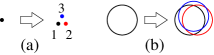
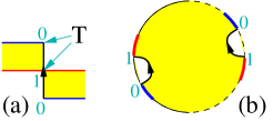
There is another way to calculate . Let be a 2D surface in space-time that describe the symmetry twist . We choose the space-time to have a form where is the time direction. At each time slice, the surface of symmetry twist, , becomes loops in the space . Then (see Fig. 1)
| (11) |
as we go around the time loop . (Such a result leads to the picture in LABEL:LG1220.)

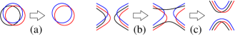
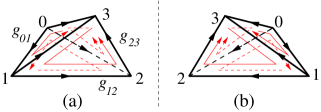
To show the relation between eqn. (10) and eqn. (I.3.2), we split each point on into three points 1, 2, 3 (see Fig. 2), which split into three nearby 2D surfaces , , and . Then from Fig. 3, we can see the relation between eqn. (10) and eqn. (I.3.2).
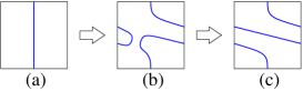
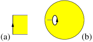
Eqn. (I.3.2) is consistent with the result in LABEL:HW1339 where we considered a space-time , where is an 1D line segment for time . Then we added a symmetry twist on a torus at (see Fig. 4a). Next, we evolved such a -twist at to the one described by Fig. 4c at , via the process Fig. 4a Fig. 4b Fig. 4c. Last, we clued the tori at and at together to form a closed space-time, after we do a double Dehn twist on one of the tori. LABEL:HW1339 showed that the value of the topological invariant on such a space-time with such a -twist is non-trivial: mod 2, through an explicit calculation. In this paper, we see that the non-trivial value comes from the fact that there is one line-reconnection in the process Fig. 4a Fig. 4b Fig. 4c.
Using the result eqn. (I.3.2), we can show that the end of the -symmetry twist line (which is called the monodromy defectWen (2014)) must carry a fractional spin mod 1 and a semion fractional statistics.Levin and Gu (2012)
Let us use to represent the many-body wave function with a monodromy defect. We first consider the spin of such a defect to see if the spin is fractionalized or not.Fidkowski et al. (2006); Wang (2010) Under a rotation, the monodromy defect (the end of -twist line) is changed to . Since and are alway different even after we deform and reconnect the -twist lines, is not an eigenstate of rotation and does not carry a definite spin.
To construct the eigenstates of rotation, let us make another rotation to . To do that, we first use the line reconnection move in Fig. 1c, to change . A rotation on gives us .
We see that a rotation changes to . We find that is the eigenstate of the rotation with eigenvalue , and is the other eigenstate of the rotation with eigenvalue . So the defect has a spin , and the defect has a spin .

If one believes in the spin-statistics theorem, one may guess that the defects and are semions. This guess is indeed correct. Form Fig. 5, we see that we can use deformation of -twist lines and two reconnection moves to generate an exchange of the two defect and a rotation of one of the defect. Such operations allow us to show that Fig. 5a and Fig. 5e have the same amplitude, which means that an exchange of two defects followed by a rotation of one of the defect do not generate any phase. This is nothing but the spin-statistics theorem.
The above understanding of geometric meaning of the topological invariant in terms of -twist domain wall also leads to a mechanism of the SPT state. Consider a quantum Ising model on 2D triangle lattice
| (12) |
where are the Pauli matrices and are nearest neighbors. Such a model can be described by the path integral of the domain walls between and in space-time. However, all domain walls in space-time have an amplitude of .
In order to have the non-trivial SPT state, we need to modify the domain wall amplitudes in the path integral to allow them to have values . The is assigned based on the following rules: as time evolves, a domain-wall-loop creation/annihilation will contribute to a to the domain-wall amplitude. A domain-wall-line reconnection will also contribute to a to the domain-wall amplitude. Those additional ’s can be implemented through local Hamiltonian. We simply need to modify the term which create the fluctuations of the domain-walls:
| (13) |
where is the sum over all six spins neighboring the site-. (In fact, we can set ). The factor contributes to a when the spin flip generated by creates/annihilates a small loop of domain walls or causes a reconnection of the domain walls. The factor contributes to a when the spin flip only deform the shape of the domain walls. This is the Hamiltonian obtained in LABEL:LG1220.

Now let us switch to the 4+1D SPT described by (see Appendix I)
| (14) |
which is a new mixed SPT phase first discovered in this paper. Here is the natural map that maps to (see Appendix E and also eqn. (5)). We note that mod 2. Hence we can rewrite if we concern about mod 2 numbers. The above topological invariant can be rewritten as
| (15) |
One of the physical properties of such a SPT state is its dimension reduction: we put the state on space-time and choose the -twist to create two identical monodromy defects on (see Fig. 6). (The physics of two identical monodromy defects was discussed in detail in LABEL:W1447 and here we follow a similar approach. Also we may embed into and view the monodromy defect as the -flux.) For such a design of and , we have mod 2 (see Fig. 6). We then take the large limit, and examine the induced the effective theory on . The induced effective Lagrangian must have a form with mod 2, which describes a topologically ordered state with chiral central charge . If has a boundary, the boundary will carry the gapless chiral edge state of chiral central charge .
We like to remark that adding two monodromy defects to is not a small perturbation. Inducing a bosonic quantum Hall state on by a large perturbation on does not imply the parent state on to be non-trivial. Even when the parent state is trivial, an large perturbation on can still induce a state on . However, what we have shown is that two identical monodromy defects on induce an odd numbers of states on . This can happen only when the parent state on is non-trivial.
We may choose another dimension reduction by putting the state on space-time and adding a -twist by threading a -flux line through the . We then take the large limit. The effective theory on will be described by effective Lagrangian . When has a boundary, , the system on the must has chiral central charge mod 8. In order words, if the 4-dimensional space has a 3-dimensional boundary and if we thread a -flux line through the , then the state on will have a gravitational response described by a gravitational Chern-Simons effective Lagrangian , with mod 2. Such a state on is either gapless or have a non-trivial topological order, regardless if the symmetry is broken on the boundary or not.
Let us assume that the SPT state has a gapped symmetry breaking boundary. The above result implies that if we have a symmetry breaking domain wall on , then the induced boundary state on must be topologically ordered with a chiral central charge mod 8. (The mod 8 comes from the possibility that the modified the local Hamiltonian at the domain wall may add several copy of bosonic quantum Hall states.) We see that a symmetry breaking domain wall on the boundary carries a 2+1D topologically ordered state with a chiral central charge mod 8.
| generators | ||
|---|---|---|
| 0 | ||
| 0 | ||
| , | ||
| 0 | ||
| , | ||
| generators | ||
| , | ||
| , , , | ||
| , , , | ||
| , , | ||
| , , |
| generators | ||
| , , | ||
| , , | ||
| , , , | ||
| , , | ||
| , , |
I.3.3 , , and SPT states in Tables 5, 6, and 7
The tables 5, 6, and 7 list the so called realizable topological invariants, which can be produced via our NLM construction. The potential topological invariants (which may or may not be realizable) for those symmetries have been calculated in LABEL:K1459v2 using cobordism approach and in LABEL:F1478 using spectrum approach. For the topological invariants that generate the classes, our realizable topological invariants agree with the potential topological invariants obtained in LABEL:K1459v2. For the topological invariants that generate the classes, our realizable topological invariants only form a subset of the potential topological invariant obtained in LABEL:K1459v2 and in LABEL:F1478.
In 1+1D, all those time-reversal protected SPT phases contain one described by
| (16) |
Here, we would like to remark that time-reversal symmetry and space-time mirror reflection symmetry should be regarded as the same symmetry.Kapustin (2014, bove) If a system has no time reversal symmetry, then we can only use orientable space-time to probe it. Putting a system with no time reversal symmetry on a non-orientable space-time is like adding a boundary to the system. If a system has a time reversal symmetry, then we can use non-orientable space-time to probe it, and in this case, the -twist is described by . Since only on non-orientable manifolds, the -twist is non-trivial only on non-orientable manifolds. So we should use a non-orientable space-time to probe the above time-reversal protected SPT phase. In fact, the above topological invariant can be detected on : mod 2 (see Fig. 7).

In the following we will explain how the above topological invariant ensure the degenerate ground states at the boundaries of 1D space. We first consider the partition of a single boundary point over a time loop (see Fig. 8a). Such a partition function on is defined by first extending into a sphere with a hole (see Fig. 8b), and then we use the 1+1D partition function defined on (from the path integral of ) to define the partition function on . We find that such a partition function on is trivial .
Now, we like to consider the partition of a single boundary point over a time loop , but now with two time-reversal transformations inserted (see Fig. 9a), where the time-reversal is implemented as mirror reflection in the transverse direction. Next, we extend Fig. 9a into a with a hole (see Fig. 9b). Since (after taking the small hole limit) mod 1, we find that the partition function on with two time-reversal transformations is non-trivial . This implies that when acting on the states on a single boundary point. The states on a single boundary must form Kramers doublets, and degenerate.
From the Tables 5, 6, and 7, we also see that most generators of 3+1D time-reversal SPT states are pure SPT states described by . All mixed time-reversal SPT states are generated by a single generator
| (17) |
which is a mixed SPT state.Vishwanath and Senthil (2013) In other words, all mixed time-reversal SPT states can be obtained from the pure SPT states by stacking with one copy of the above mixed SPT state.
I.3.4 SPT states in Table 8
| generators | ||
| , | ||
| , , | ||
| , , , | ||
| , , | ||
| , , , , |
The 1+1D SPT state is characterized by the following topological invariant
| (18) |
Let us explain how such a topological invariant ensure the degenerate ground states at the boundaries of 1D space. Let us consider a 1+1D space-time which is with a small hole (see Fig. 8b). The partition function for can be viewed as the effective theory for the boundary , which is the partition function for a single boundary point of 1D space over the time loop (see Fig. 8a). Since the partition function on changes sign as we add flux to , this means that a rotation acting on the states on a single boundary point will change the sign of the states. So the states on a single boundary point must form a projective representation of where the rotation is represented by . Such a projective representation is alway even dimensional, and the states on a single boundary point must have an even degeneracy.
From the 2+1D topological invariants, we see that the 2+1D SPT is actually the 2+1D SPT state (by ignoring ) and the 2+1D SPT state (by ignoring ).
In 3+1D, we have a pure 3+1D SPT state described by
| (19) |
which is a SPT state for quantum spin systems.
To construct a physical probe for the above SPT state, we first note that the topological invariant (19) is invariant under time reversal (mod ). So the corresponding SPT state is compatible with time reversal symmetry. If we assume the SPT state also have the time reversal symmetry, then we can design the following probe for the SPT state. We choose the 3+1D space-time to be , and put flux through , where is actually a lattice. But such flux is in a form a two identical thin -flux and each -flux going through a single unite cell in . Such a configuration has mod 2, and at the same time, does not break the symmetry.
In the large limit, the dimension-reduced theory on is described by a topological invariant . However, due to an identity in 2-dimensional space, mod 2, if is orientable (since iff the manifold is orientable). The topological invariant can be detected only on non-orientable . This is where we need the time reversal symmetry: in the presence of time reversal symmetry, we can use non-orientable to probe the topological invariant.
Let be the symmetry group generated by the combined transformation and time-reversal transformation. Let be the -twist. Then we have . Thus the topological invariant can be rewritten as , which describes a 1+1D SPT state protected by time reversal symmetry .
We like to remark that threading two thin -flux lines through is not a small perturbation. Inducing a SPT state on by a large perturbation on does not imply the parent state on to be non-trivial. Even when the parent state is trivial, an large perturbation on can still induce a SPT state on . However, what we have shown is that threading two identical thin -flux lines through induces one SPT state on . This can happen only when the parent state on is non-trivial.
I.4 Realizable and potential topological invariants
After discussing the physical consequences of various topological invariants,
let us turn to study the topological invariants themselves. It turns out that
the topological invariants for iTO states satisfy many self consistent
conditions. Solving those conditions allow us to obtain self consistent
topological invariants, which will be called potential gauge-gravity
topological invariants. LABEL:K1467,K1459v2,KTT1429,F1478,WGW1489 studied the
topological invariants from this angle and only the potential gauge-gravity
topological invariants are studied. For example, when there is no symmetry,
the following type of potential gauge-gravity topological invariants were
found:
(1) The 2+1D potential gravitational topological invariants are described by
,Kane and Fisher (1997); Hughes et al. (2012); Plamadeala et al. (2013); Kong and Wen (2014) which are generated by
| (20) |
where is the gravitational Chern-Simons term that is defined via , with the Pontryagin class. In LABEL:F1478, it was suggested that the 2+1D potential gravitational topological invariants are generated by
| (21) |
(2) The 4+1D potential gravitational topological invariants are described by ,Kapustin (2014, bove); Kong and Wen (2014) which are generated by
| (22) |
where is the Stiefel-Whitney class.
(3)
The 6+1D potential gravitational topological invariants are described by
,Kong and Wen (2014)
which are generated by
| (23) |
where the gravitational Chern-Simons terms are defined by and .
The potential topological invariants in eqn. (20), eqn. (22), and eqn. (I.4) have a close relation to the orientated -dimensional cobordism group ,Kapustin (2014, bove); Kapustin et al. (2014) which are Abelian groups generated by the Stiefel-Whitney classes and the Pontryagin classes . For example, is generated by the Pontryagin class and by and . Also is generated by Stiefel-Whitney class . In this case, the set of potential gravitational topological invariants in -dimensional space-time (denoted as ) are exactly those Stiefel-Whitney classes and the Pontryagin classes that describe the cobordism group :
| (24) |
Note that and are discrete Abelian groups. Tor and Free are the torsion part and the free part of the discrete Abelian groups.
However, we do not know if those potential gauge-gravity topological invariant can all be realized or produced by local bosonic systems. In this paper, we will study this issue. However, to address this issue, we need to first clarify the meaning of “realizable by local bosonic systems”.
We note that there are two types of local bosonic systems: L-type and H-type.Kong and Wen (2014) L-type local bosonic systems are systems described by local bosonic Lagrangians. L-type systems have well defined partition functions for space-time that can be any manifolds. H-type local bosonic systems are systems described by local bosonic Hamiltonians. H-type systems have well defined partition functions only for any space-time that are mapping tori. (A mapping torus is a fiber bundle over .) A L-type system always correspond to a H-type system. However, a H-type system may not correspond to a L-type system. For example, SPT phases described by group cohomology and the NLMs are L-type topological phases (and they are also H-type topological phases). The bosonic quantum Hall state is defined as a H-type topological phase. However, it is not clear if it is a L-type topological phase or not. In the following, we will argue that any quantum Hall state is also a L-type topological phase (i.e. realizable by space-time path integral, that is well defined on any space-time manifold).
In this paper, we will only consider L-type bosonic quantum systems. We will study which potential gauge-gravity topological invariants are realizable by L-type local bosonic systems. We will use NLMs (1) to try to realize those potential gauge-gravity topological invariants. After adding the -symmetry twist and choose a curved space-time , the “gauged” NLMs (1) becomesHung and Wen (2012, 2013b); Wen (2013)
| (25) |
where the space-time connection couples to and the “gauge” connection couples to . The induced gauge-gravity topological term is classified by group cohomology . After we integrate out the matter fields , the above gauged NLM will produce a partition function that give rise to a realizable gauge-gravity topological invariant via
| (26) |
(See LABEL:W8570 for a study of gauged topological terms described by Free for continuous groups.)
The set of potential gauge-gravity topological terms contain the set of realizable gauge-gravity topological terms. More precisely, the two sets are related by a map
| (27) |
However, the map may not be one-to-one and may not be surjective.
For example, when there is no symmetry, we find that the following type of
realizable gauge-gravity topological invariants were generated by the above NLM
(see Table 1):
(1) Those 2+1D realizable gravitational topological invariants are described by
, which are generated by
| (28) |
The corresponding generating topological state has a chiral central charge
at the edge. So the stacking of three bosonic quantum Hall states
can be realized by a well defined L-type local bosonic system. It is not clear
if a single bosonic quantum Hall state can be realized by a L-type local
bosonic system or not. However, we know that a single bosonic quantum
Hall state can be realized by a H-type local bosonic system.
(2) Those 4+1D
realizable gravitational topological invariants are described by
,
which are generated by
| (29) |
(Note that is also in this case.) In fact, we will show
that all the potential gauge-gravity topological invariants that generate a finite
group are realizable by the NLMs,
which are L-type local bosonic systems.
(3) , and there are four different types of
NLMs (with four different topological terms). However, the four different
topological terms in the NLMs all reduce to the same trivial gravitational
topological invariant after we integrate out the matter field
, suggesting that all the four NLMs give rise to the same topological
order.
(4)
Those 6+1D realizable gravitational topological invariants are described by ,
which are generated by
| (30) |
We see that only part of the potential gravitational topological invariants are realizable by the NLMs.
However, it is possible that NLMs do not realize all possible L-type iTO’s. In the following, we will argue that the 2+1D bosonic quantum Hall state is a L-type iTO. NLM cannot realize the state since it has a central charge and a topological invariant .
In fact, we will argue that any quantum Hall state is a L-type topologically ordered state. Certainly, by definition, any quantum Hall state, being realizable by some interacting Hamiltonians, is a H-type topologically ordered state. The issue is if we can have a path-integral description that can be defined on any closed space-time manifold. At first, it seems that such a path-integral description does not exist and a quantum Hall state cannot be a L-type topological order. This is because quantum Hall state is defined with respect to a non-zero background magnetic field – an closed two-form field () in 2+1D space-time. This seems imply that a path-integral description of quantum Hall state exist only on space-time that admits a every-where non-zero closed two-form field.
However, as stressed in LABEL:WW0808,WW0809, a quantum Hall state of filling fraction always contains an -cluster structure. Also, the closed two-form field in 2+1D space-time may contain “magnetic monopoles”. If those “magnetic monopoles” are quantized as multiples of , they will correspond to changing magnetic field by flux quanta each time. Changing magnetic field by flux quanta and changing particle number by -clusters is like adding a product state to a gapped quantum liquid discussed in LABEL:ZW1490, which represents a “smooth” change of the quantum Hall state. Since every-where non-zero closed two-form field with “magnetic monopoles” can be defined on any 2+1D space-time, we can have a path-integral description of any quantum Hall state, such that the path-integral is well defined on any space-time manifold. We conclude that quantum Hall states, such as the state, are L-type topologically ordered states. Therefore, the gravitational topological invariant
| (31) |
is realizable by a 2+1D L-type iTO, i.e. a state (see Table 1).
I.5 A construction of L-type realizable pure and mixed SPT phases
Now, let us include symmetry and discuss SPT phases (i.e. L-type topological phases with short range entanglement). We like to point out that some SPT states are characterized by boundary effective theory with anomalous symmetry,Wen (2013); Kapustin and Thorngren (2014, 2014) which is commonly referred as gauge anomaly (or ’t Hooft anomaly). Those SPT states are classified by group cohomology of the symmetry group . We also know that the boundaries of topologically ordered statesWen (1989); Wen and Niu (1990); Wen (1990); Keski-Vakkuri and Wen (1993) realize and (almost111For example, the pure 2+1D gravitational anomalies described by unquantized thermal Hall conductivity are not classified by topologically ordered states.) classify all pure gravitational anomalies.Kong and Wen (2014) So one may wonder, the boundary of what kind of order realize mixed gauge-gravity anomalies? The answer is SPT order. This is because the mixed gauge-gravity anomalies are present only if we have the symmetry. Such SPT order is also beyond the description, since the mixed gauge-gravity anomalies are beyond the pure gauge anomalies. We will refer this new class of SPT states as mixed SPT states and refer the SPT states with only the pure gauge anomalies as pure SPT states. We would like to mention that the gauge anomalies and mixed gauge-gravity anomalies have played a key role in the classification of free-electron topological insulators/superconductors.Ryu et al. (2009, 2012)
The main result of this paper is a classification of both pure and mixed SPT states realized by the NLMs:
| (32) | ||||
where is the Abelian group formed by the L-type SPT phases in -dimensional space-time produced by the NLMs, and is the Abelian group formed by the L-type iTO phases in -dimensional space-time produced by the NLMs. Also is a subgroup of .
Replacing by – the Abelian group formed by the L-type iTO phases in -dimensional space-time, we obtain more general SPT states described by :
(33)
If contains time-reversal transformation, it will have a non-trivial action and . Also, is the classifying space of and is the topological cohomology class on .
Note that stacking two topological phases and together will produce another topological phase . We denote such a stacking operation as . Under , the topological phases form a commutative monoid.Kong and Wen (2014) In general, a topological phase may not have an inverse, i.e. we can not find another topological phase such that is a trivial product state. This is why topological phases form a commutative monoid, instead of an Abelian group. However, a subset of topological phases can have inverse and form an Abelian group. Those topological phases are called invertible.Kong and Wen (2014); Freed (2014) One can show that a topological phase is invertible iff it has no topological excitations.Kong and Wen (2014); Freed (2014) Therefore, all SPT phase are invertible. Some topological orders are also invertible, which are called invertible topological orders (iTO). SPT phases and iTO phases form Abelian groups under the stacking operation. So for SPT states and iTO states, we can replace by :
| (34) |
So and can be viewed as modules over the ring , and they can appear as the coefficients in group cohomology.
The result (32) can be understood in two ways. It means that the SPT states constructed from NLMs are all described by , but in a many-to-one fashion; i.e. contain a subgroup that different elements in correspond to the same SPT state. It also means that the constructed SPT states are described by , but in a one-to-many fashion; i.e. each element of correspond to several SPT states that form a group . The group and can be calculated but we do not have a simple expression for them (see Section V).
In eqn. (33), includes both pure and mixed SPT states. The group cohomology class describes the pure SPT phases, and the group cohomology class describes the mixed SPT phases. We would like to mention that an expression of the form eqn. (33) was first proposed in LABEL:W1447 in a study of topological invariants of SPT states. We see that our NLMs construction can produce mixed SPT phases with and without time reversal symmetry. We have used eqn. (33) to compute the SPT phases for some simple symmetry groups (see Table 2).
The formal group cohomology methods employed for obtaining the result (33) directly shed light on the physics of these phases. The SPT states described by in eqn. (33) can be constructed using the decorated domain walls proposed in LABEL:CLV1407. Other SPT states described can be obtained by a generalization of the decorated-domain-wall construction,Liu et al. (2014b); Wang et al. (2014b); Gu et al. (2015) which will be called the nested construction.Gu and Wen (2014) The formal methods also lead to physical/numerical probes for these phases.Levin and Gu (2012); Vishwanath and Senthil (2013); Metlitski et al. (2013); Wen (2014); Ye and Wen (2014); Bi et al. (2014); Wang et al. (2014a) In addition, these methods are easy to generalize to fermionic systemsGu and Wen (2012, 2014), and provide answers for the physically important situation of continuous symmetries (like charge conservation).
We also studied the potential SPT phases (i.e. might not realizable) for a non-on-site symmetry – the mirror-reflection symmetry . The Abelian group formed by those SPT phases is denoted as . Following LABEL:K1467,K1459v2,KTT1429, we find that is given by a quotient of the unoriented cobordism groups
(35)
where is the orientation invariant subgroup of (i.e. the manifold and its orientation reversal belong to the same oriented cobordism class). It is interesting to see
| (36) |
(see Table 5).
We want to remark that, in this paper, the time reversal transformation is defined as the complex conjugation transformation (see Section II.2), without the transformation. The mirror reflection correspond to the transformation. The time-reversal symmetry used in LABEL:K1467,HMC1402,K1459v2,KTT1429 is actually the mirror-reflection symmetry in this paper. The two ways to implement time-reversal symmetry should lead to the same result as demonstrated by eqn. (36), despite the involved mathematics, the cobordism approach and NLM approach, are very different.
I.6 Discrete gauge anomalies, discrete mixed gauge-gravity anomalies, and invertible discrete gravitational anomalies
First, let us explain the meaning of discrete anomalies. All the commonly known anomalies are discrete in the sense that different anomalies form a discrete set. However, there are continuous gauge/gravitational anomalies labeled by one or more continuous parameters.Wen (2013); Kong and Wen (2014) In this section, we only consider discrete anomalies.
Since the boundaries of SPT states realize all pure gauge anomalies, as a result, group cohomology systematically describe all the perturbative and global gauge anomalies.Wen (2013); Kapustin and Thorngren (2014) For topological orders, we found that they can be systematically described by tensor category theoryFreedman et al. (2004); Levin and Wen (2005); Chen et al. (2010); Gu et al. (2010); Kitaev and Kong (2012); Gu et al. (2013); Kong and Wen (2014) and tensor network,Verstraete and Cirac (2004); Gu et al. (2009); Buerschaper et al. (2009) and those theories also systematically describe all the perturbative and global gravitational anomalies.Kong and Wen (2014)
Or more precisely, the discrete pure bosonic gauge anomalies in -dimensional space-time are described by . The discrete invertible pure bosonic gravitational anomalies in -dimensional space-time are described FreeTor. The discrete mixed bosonic gauge-gravity anomalies are described by .
In Table 1, we list the generators of the topological invariants . Those topological invariants describe various bosonic invertible gravitational anomalies in one lower dimension. For example, describes the well known perturbative gravitational anomaly in 1+1D chiral boson theories. The topological invariant implies a new type of bosonic global gravitational anomaly in 4+1D bosonic theories. In Tables 3, 4, 6, 7, 5, 8, we list the generators of the topological invariants for some simple groups. Those topological invariants describe various bosonic anomalies for those groups at one low dimensions. For example, describes the well known perturbative gauge anomaly in 1+1D chiral boson theories. The topological invariant implies a new type of bosonic global gauge anomaly in 2+1D bosonic theories. In fact, all the non--type topological invariants in the Tables give rise to new type of bosonic global gauge/gravity/mixed anomalies in one lower dimension.
Note that the invertible anomalies are the usual anomalies people talked about. They can be canceled by other anomalies. The anomalies, defined by the absence of well defined realization in the same dimension, can be non-invertible (i.e. cannot be canceled by any other anomalies).Kong and Wen (2014) All pure gauge and mixed gauge-gravity anomalies are invertible, but most gravitational anomalies are not invertible.Kong and Wen (2014)
I.7 The relations between the H-type and the L-type topological phases
We have introduced the concept of potential SPT phases (which may or may not be realizable), H-type SPT phases (which are realizable by H-type local quantum systems), and L-type SPT phases (which are realizable by L-type local quantum systems). Those SPT phases are related
| (37) |
where represents subgroup and is a group homomorphism. Similarly, we also introduced the concept of potential iTO phases (which may or may not be realizable), H-type iTO phases (which are realizable by H-type local quantum systems), and L-type iTO phases (which are realizable by L-type local quantum systems). Those iTO phases are related
| (38) |
In condensed matter physics, we are interested in and . (A study on the H-type topological phases can be found in LABEL:KW1458,F1478.) But in this paper, we will mainly discuss and . The SPT states constructed in LABEL:CLW1141,CGL1314,CGL1204 belong to (and they also belong to ). The SPT states constructed in LABEL:VS1306,WS1334,BCF1372,XY1486 belong to . In LABEL:K1467,K1459v2,KTT1429,F1478,WGW1489 only the potential SPT states are studied.
I.8 The organization of this paper
In Section II, we review the NLM construction of the pure SPT states. In Section III, we generalize the NLM construction to cover the mixed SPT states and iTO states. In Section IV, a construction L-type iTO orders is discussed. Using such a construction Section V, we proposed a construction the pure and the mixed SPT states of the L-type. In Section VI, we discussed the L-type SPT states protected by the mirror reflection symmetry.
II Group cohomology and the L-type pure SPT states
A L-type pure SPT state in -dimensional space-time can be realized by a NLM with the symmetry group as the target space
| (39) |
in large limit. Here we treat the space-time as a (random) lattice which can be viewed as a -dimensional complex. The space-time complex has vertices, edges, triangles, tetrahedrons etc. The field live on the vertices and live on the edges. So is in fact a sum over the vertices, edges, and other simplices of the lattice. is the lattice difference between vertices connected by edges. The above action actually defines a lattice theory.Chen et al. (2013, 2012)
Under renormalization group transformations, flows to infinity. So the fixed point action contains only the topological term. In this section, we will describe such a fixed-point theory on a space-time lattice.Levin and Gu (2012); Moore and Read (1991); Hung and Wen (2013b). The space-time lattice is a triangulation of the space-time. So we will start by describing such a triangulation.
II.1 Discretize space-time
Let be a triangulation of the -dimensional space-time. We will call the triangulation as a space-time complex, and a cell in the complex as a simplex. In order to define a generic lattice theory on the space-time complex , it is important to give the vertices of each simplex a local order. A nice local scheme to order the vertices is given by a branching structure.Costantino (2005); Chen et al. (2013, 2012) A branching structure is a choice of orientation of each edge in the -dimensional complex so that there is no oriented loop on any triangle (see Fig. 10).
The branching structure induces a local order of the vertices on each simplex. The first vertex of a simplex is the vertex with no incoming edges, and the second vertex is the vertex with only one incoming edge, etc . So the simplex in Fig. 10a has the following vertex ordering: .
The branching structure also gives the simplex (and its sub simplices) an orientation denoted by . Fig. 10 illustrates two -simplices with opposite orientations and . The red arrows indicate the orientations of the -simplices which are the subsimplices of the -simplices. The black arrows on the edges indicate the orientations of the -simplices.
II.2 NLM on a space-time lattice
In our lattice NLM, the degrees of freedom live on the vertices of the space-time complex, which are described by where labels the vertices.
The action amplitude for a -cell is a complex function of : . The total action amplitude for a configuration (or a path) is given by
| (40) |
where is the product over all the -cells . Note that the contribution from a -cell is or depending on the orientation of the cell. Our lattice NLM is defined by following imaginary-time path integral (or partition function)
| (41) |
where the action amplitude is invariant or covariant under the -symmetry transformation , :
| (42) |
Note that here we allow to contain time-reversal symmetry. In H-type theory (i.e. in Hamiltonian quantum theory) the time-reversal transformation is implemented by complex conjugation without reversing the time (there is no time to reverse in Hamiltonian quantum theory). Generalizing that to L-type theory, we will also implement time-reversal transformation by complex conjugation without reversing the time . This is the implementation used in LABEL:CGL1314,CGL1204. in eqn. (42) describes the effect of complex conjugation. if contains no time-reversal transformation and if contains a time-reversal transformation.
The fixed-point theory contains only the pure topological term. Such a pure topological term can be constructed from a group cocycle . Note that a group cocycle is a map from to (see Appendix A). We can express the action amplitude that correspond to a pure topological term asChen et al. (2013, 2012)
| (43) |
Due to the symmetry condition (182), the action amplitude is invariant/covariant under the -symmetry transformation. Due to the cocycle condition (184), the total action amplitude on a closed space-time is always equal to 1:
| (44) |
Also two cocycles different by a coboundary (see eqn. (185)) can be smoothly deformed into each other without affecting the condition (44). In other words, the connected components of the fixed-point theories that satisfy the condition (44) are described by . This way, we show that the fixed-points of the NLMs are classified by the elements of .
We like to remark that for continuous group, the cocycle do not need to be continuous function of . It can be a measurable function.
II.3 Adding the -symmetry twist
The above bosonic system may be in different SPT phases for different choices of the topological term (i.e. for different choices of group cocycles ). But how can we be sure that the system is indeed in different SPT phases? One way to address such a question is to find measurable topological invariants, and show that different cocycles give rise to different values for the topological invariants.
In this section, we will assume that the symmetry group does not contain time-reversal. In this case, the universal topological invariants for SPT state can be constructed systematically by twisting (or “gauging”) the on-site symmetry Levin and Gu (2012); Hung and Wen (2012); Hu et al. (2013); Hung and Wen (2013b) and study the gauged bosonic model
| (45) |
Note that the gauge field just represents space-time dependent coupling constants, which is not dynamical (i.e. we do not integrate out the gauge field in the path integral). Since the SPT state is gapped for large , in large space-time limit, the partition function has a form
| (46) |
where is the ground state energy density and is the volume of the space-time manifold . The term represents the volume independent term in the partition function and is conjectured to be universal (i.e. independent of any small local change of the Lagrangian that preserve the symmetry).Kong and Wen (2014) Such a term is called the realizable gauge topological term (or topological invariant), which is referred as the SPT invariant in LABEL:W1447,HW1339. The SPT invariants are the topological invariants that are believed to be able to characterize and distinguish any SPT phases.
The topological invariant is gauge invariant, i.e. for any closed space-time manifold
| (47) |
where we have treated as the gauge field one form. Also, as a topological invariant, does not dependent on the metrics of the space-time. For example can be a Chern-Simons term in 2+1D or a -term in 3+1D. The presence of non-trivial topological invariant indicates the presence of non-trivial SPT phase.
In the above, we described the symmetry twist in the continuous field theory. On lattice, the symmetry twist can be achieved by introducing for each edge in the space-time complex . The twisted theory (i.e. the “gauged” theory) is described by the total action amplitude
| (48) |
The imaginary-time path integral (or partition function) is given by
| (49) |
We see that only are dynamical. are non-dynamical background probe fields. The above action amplitude on closed space-time complex () should be invariant under the “gauge” transformation
| (50) |
and covariant under the global symmetry transformation
| (51) |
| (52) |
The gauged action amplitudes is obtained from the ungauged action amplitudes in the following way (where we assume is discrete):
| (53) |
where are given by
| (54) |
At a fixed-point, the twisted action amplitude is given by
where is the inhomogeneous cocycle corresponding to
| (55) |
By rewriting the partition function as (see eqn. (II.3))
| (56) |
we find that the partition function is explicitly gauge invariant and symmetric.
The topological invariant is given by the fixed-point partition function for the twisted theory
| (57) |
The twisted fixed-point partition function or is non-trivial and depend on the symmetry twist (or gauge connection ). We see that different realizable topological invariants are classified and given explicitly by the elements of group cohomology :
| (58) |
where is an inhomogeneous cocycle in , and on the edges complex define the symmetry twist in space-time . Eq. (58) tells us how to calculate , given cocycle , the space-time manifold , and the symmetry-twist .
We can also see this within the field theory. The realizable gauge topological invariant and the NLM topological term are directly related:
| (59) |
Since the NLM topological terms are classified by the group cohomology of the symmetry group . The realizable gauge topological invariants are also classified by .
The gauge topological term (or topological invariant) can be defined for both continuous and discrete symmetry groups . In general, it is a generalization of the Chern-Simons term.Dijkgraaf and Witten (1990); Hung and Wen (2012); Hu et al. (2013) It describes the response of the quantum ground state. We hope that the ground states in different quantum phases will produce different responses, which correspond to different classes of gauge topological terms, that cannot be smoothly deformed into each other. So we can use such a term to study and classify pure SPT phases.
We would like to point out that there are two kinds of topological invariants.
The topological invariants correspond to Tor
are called locally-null topological invariants.
They have the following defining properties:
(1) are well defined for any symmetry twists .
(2) does not depend on any small smooth change
of the symmetry twist:
| (60) |
The topological invariants correspond to Free are called Chern-Simons topological invariants. The Chern-Simons topological invariants is only well defined for some symmetry twists . In general, only the difference
| (61) |
is well defined, provided that there exist an -dimensional manifold such that and the gauge connections on and on can be extended to (see Appendix B).
Now two questions naturally arise:
(1) how to write down the most general topological invariants
(i.e. the most general topological invariants) which are
self consistent? We will call such topological invariants as potential
topological invariants.
(2) can we show that every potential topological invariant can be induced by
some symmetric local bosonic model, after we gauge the on-site symmetry?
In Appendix B, we will
address these two questions. We find that the potential gauge topological
invariants are described by ,
which are all realizable since .
II.4 pure SPT states
In this section, we will study pure SPT states described by group cohomology . This result will be useful for later discussions. First, we can use the following version of Künneth formulaWen (2013, 2014)
| (62) |
to compute . In addition, the above Künneth formula can help us to construct topological invariants to probe the SPT order.Wen (2014)
For example, a SPT order in -dimensional space-time can be probed by a map , that maps a closed space-time with a -symmetry twist to a number in :
| (63) |
Such a map is nothing but the topological invariant that we discussed before. At the same time, the topological invariant can also be viewed as a cocycle in , since it is a map for the -bundles (i.e. the -symmetry twists) on to , and the -bundles on is classified by the embedding of into the classifying space. Different SPT states will lead to different maps. We believe that the map fully characterizes the SPT states described by (see Appendix B).Wen (2014); Hung and Wen (2013a)
Similarly, for the pure SPT states described by , they can also be probed by a map , that maps a closed space-time with a -symmetry twist on to an element in . This is simply a dimension reduction: we consider a pace-time of the form , add a -symmetry twist on , and then take a large limit. The system can be viewed as a -dimensional SPT state on , which is described by an element in . Such a dimension reduction can be formally written as
| (64) |
which has the same structure as eqn. (63). The map can be viewed as a cocycle in . Such a map fully characterizes the pure SPT states described by .
The dimension reduction discussed above reveals the physical meaning of the Künneth formula. We will use such a physical picture to obtain the key result of this paper.
III Constructing pure and mixed SPT states, as well as iTO states
III.1 SPT states, gauge anomalies and mixed gauge-gravity anomalies
So far, we have reviewed the group cohomology approach to pure SPT states. It was pointed out in LABEL:W1313 that (a) the SPT orders (described by ) and pure gauge anomalies in one lower dimension are directly related and (b) the topological orders and gravitational anomalies in one lower dimension are directly related. This suggests that the SPT orders beyond Vishwanath and Senthil (2013); Wang and Senthil (2013); Burnell et al. (2013); Kapustin (2014, bove); Wang et al. (2014b); Xu and You (2014) and mixed gauge-gravity anomalies are closely related.Wang et al. (2014b) This line of thinking gives us a deeper understanding of generic SPT states. In this section, we are going to construct local bosonic models that systematically realize iTO’s, pure SPT orders (associated with pure gauge anomaly), and mixed SPT orders (associated with mixed gauge-gravity anomaly).
III.2 Realizable L-type SPT and iTO phases
One of the key properties of SPT states is that they do not contain any non-trivial topological excitations.Chen et al. (2011c, 2013, 2012) In LABEL:KW1458 it was conjectured that a gapped quantum liquid state has no non-trivial topological excitations iff its fixed-point partition function is a pure phase.
However, when we study the pure SPT orders described by using NLMs, we only add the symmetry twists, which are associated with the -bundles on the space-time, to induce the non-trivial -phase-valued partition function. This is why we only get pure gauge anomalies in such an approach. To get the gravitational anomalies and the mixed gauge-gravity anomalies, we must include the space-time twist, described by the non-trivial tangent bundle of the space-time as well. The tangent bundle is a bundle. Thus to include the gravitational anomalies and the mixed gauge-gravity anomalies, as well as the pure gauge anomalies, we simply need to consider a NLM with topological term where . We can gauge the symmetry to probe the SPT states and the pure gauge anomalies as before. We can also choose non-flat space-time to probe the SPT states (and the gravitational anomalies), that corresponds to couple the part of the NLM to the connection of the tangent bundle of the space-time. We will see that using NLMs, we can obtain a topological invariant that contains both the gauge -connection and the gravitational -connection . Such kind of bosonic NLM is capable of producing the pure SPT states that are associated with pure gauge anomalies, as well as the mixed SPT states that are associated with mixed gauge-gravity anomalies. It can also produce iTO states, if we choose a trivial symmetry group .
Here we would like to remark that we can also use an NLM with to produce the SPT states and iTO states. The stability consideration suggests the we should take . So we will use NLM to study the new topological states, where .
Repeating the discussion in Section II.2, we find that the realizable gauge-gravity topological invariants in the NLM can be constructed from each element in the group cohomology class . However, because of the restrictive relation between the gravitational connection and the topology of the space-time (see Appendix C), the correspondence is not one-to-one: different elements in may produce the same realizable gauge-gravity topological invariant after integrating out the matter field . The reason is the following. For two topological invariants and obtained from two cocycles and in , it is possible that
| (65) |
on any closed space-time . In this case, we should view and as the same topological invariant. (Note that the above two topological invariants can be distinguished if the connection is not restricted to be the connection of the tangent bundle of the space-time .) Thus, contains a subgroup such that the realizable gauge-gravity topological invariants have an one-to-one correspondence with the elements in . Those different NLMs, that produce different the realizable gauge-gravity topological invariants , realize different L-type topological phases with no topological excitations.
In Appendix C, we will discuss potential gauge-gravity topological invariants . We find that the locally-null potential gauge-gravity topological invariants are described by a subgroup of , which are all realizable. We also find that Chern-Simons potential gauge-gravity topological invariants are described by a subgroup of . NLMs can only realize those that are also in .
IV iTO states
Using Pontryagin class and Stiefel-Whitney class, one can show that different L-type potential iTO phases (i.e. may not be realizable) are described by in 3-dimensions,Plamadeala et al. (2013) in 4-dimensions,Kong and Wen (2014); Kapustin (bove) and in 7-dimensions, where the dimensions are the space-time dimensions. In this section, we will reexamine those results using the approaches discussed above, and try to understand which L-type potential iTO can be realized by NLMs. We will show that the above potential topologically ordered phases described by Stiefel-Whitney class are always realizable, while only a subset of those described by Pontryagin classes are realizable by NLMs. The result is summarized in Table 1.
IV.1 Classification of NLMs
Since we do not have any symmetry, the realizable gauge-gravity topological invariants produced by the NLMs are covered by , . In Appendix D, we calculated the ring . In low dimensions, we have
| (66) | ||||
We note that due to the relation , the -dimensional gauge-gravity topological invariants (with values in ) is promoted to -dimensional topological invariants (with values in ). In the above, we also listed the basis of those topological invariants, so that a generic topological invariant is a superposition of those basis. In the following, we list and the basis of their topological invariants :
| (67) | ||||
The above basis give rise to the basis in eqn. (IV.1) through the natural map : (see Appendix E).
We see that , which implies that a realizable gauge-gravity topological invariant exist in 1+1D, provided that we probe the NLM by an arbitrary bundle on an oriented 1+1D space-time manifold :
| (68) |
where is the connection of the bundle on and are the Stiefel-Whitney classes for the bundle. However, the bundle on is restricted: it must be the tangent bundle of . So we actually have
| (69) |
where is the connection of the tangent bundle on and are
the Stiefel-Whitney classes for the tangent bundle. The Stiefel-Whitney
classes for the tangent bundle have some special relations.
In fact, we have
(1) a manifold is orientable iff .
(2) a manifold admits a spin structure iff .
Since all closed orientable 2-dimensional manifold is spin, thus both
and vanish for tangent bundles of . The realizable gauge-gravity
topological invariant cannot be probed by any oriented space-time . Thus, the
above realizable gauge-gravity topological invariants described by
collapse to zero in 1+1D. There is no iTO in 1+1D (or in other words,
).
IV.2 Relations between Stiefel-Whitney classes
We see that to understand the realizable gauge-gravity topological invariants, whether they collapse to zero or not, it is important to understand all relations that the Stiefel-Whitney classes must satisfy, when the Stiefel-Whitney classes come from a tangent bundle. To obtain such relations, let us first consider the Stiefel-Whitney classes for an arbitrary vector bundle on a -dimensional space.
We note that the total Stiefel-Whitney class is related to the total Wu class through the total Steenrod square:
| (70) |
Therefore,
| (71) |
The Steenrod squares have the following properties:
| (72) |
for any . Thus
| (73) |
This allows us to compute iteratively, using Wu formula
| (74) | ||||
and the Steenrod relation
| (75) |
We find
| (76) | ||||
We note that the Steenrod squares form an algebra:
| (77) |
which leads to the relation used in the last section.
If the vector bundle on -dimensional space, , happen to be the tangent bundle of , then the Steenrod square and the Wu class satisfy
| (78) |
(1) If we choose to be a combination of Stiefel-Whitney classes, the
above will generate many relations between Stiefel-Whitney classes.
(2) Since if , therefore for any if . Thus, for -dimensional manifold, the Wu
class if . Also if . This also
gives us relations among Stiefel-Whitney classes.
(3) Last, there is another type of relation. In -dimension, the mod 2 reduction
of Pontryagin classes , , should be
regarded as zero. The reason is explained below the eqn. (84). This lead to
the relations for -dimensional manifold
| (79) |
is given by after quotient out all those relations.
IV.3 iTO phases in low dimensions
In 2-dimensional space-time which is generated by . So may be non-trivial. The relations give us
| (80) |
Since is oriented, . We see that . vanishes, and there is no realizable gauge-gravity topological invariant in 1+1D. So .
In 2+1D space-time, the corresponding is generated by . There is no relation involving . So . The generating topological invariant describes an iTO state with chiral central charge .
In 3+1D space-time, the corresponding is generated by the gauge-gravity topological invariant . The Wu classes can lead to relations between the Stiefel-Whitney classes, which give us
| (81) |
Other relations can be obtained by applying the Steenrod squares to the above:
| (82) |
Additional relations can be obtained from eqn. (78)
| (83) | ||||
We see that , but nothing restricts . Naively, this suggests that is a realizable gauge-gravity topological invariant in 3+1D:
| (84) |
However, there is a relation between Pontryagin classes and Stiefel-Whitney classes (see Appendix F):
| (85) |
on any closed oriented manifolds of dimension . Thus is part of Pontryagin class . The topological invariant is realizable, but also smoothly connect to the trivial case via the Pontryagin class: , where can go from to smoothly. There is no realizable gauge-gravity topological invariant in 3+1D that cannot connect to zero. Thus . In general, such kind of reasoning give rise to eqn. (79).
In 4+1D space-time, the corresponding is generated by the gauge-gravity topological invariant . The Wu classes can lead to relations between the Stiefel-Whitney classes, which give us
| (86) |
is just a generator of the relations. Other relations can be obtained by applying the Steenrod squares:
| (87) |
Additional relations can be obtained from eqn. (78)
| (88) | ||||
We see that must vanishes, but nothing restricts . So we have an realizable gauge-gravity topological invariant in 4+1D:
| (89) |
Thus .
In 5+1D space-time, the corresponding is generated by the gauge-gravity topological invariant . The Wu classes give us
| (90) |
Other relations can be obtained by applying the Steenrod squares:
| (91) |
We see that must vanishes, and . Additional relations can be obtained from eqn. (78)
| (92) | ||||
We see that . So .
In 6+1D space-time, the corresponding is generated by the gauge-gravity topological invariant . The Wu classes give us
| (93) |
Other relations can be obtained by applying the Steenrod squares (setting ):
| (94) |
Additional relations can be obtained from eqn. (78) (setting ):
| (95) | ||||
We see that . So .
IV.4 Relation to cobordism groups
Two oriented smooth -dimensional manifolds and are said to be
equivalent if is a boundary of another manifold, where is
the manifold with a reversed orientation. With the multiplication given
by the disjoint union, the corresponding equivalence classes has a structure
of an Abelian group , which is called the cobordism group of
closed oriented smooth manifolds. For low dimensions, we haveOCo (2013)
, generated by a point.
, since circles
bound disks.
, since all oriented surfaces bound
handlebodies.
.
, generated by ,
detected by .
, generated by the Wu
manifold ,
. detected by the deRham invariant
or
. Stiefel-Whitney number .
.
.
generated by and .
The potential gravitational topological invariants give us a map from closed space-time to : . For locally-null topological invariants, such a map reduces to a map from to . In fact, is an 1D representation of group . So the locally-null potential gravitational topological invariants are described by 1D representations of the cobordism group . Since the locally-null potential gravitational topological invariants are discrete, so they are actually described by 1D representation of Tor. Since, for an Abelian group , the set of its 1D representations also form an Abelian group, which is itself. Therefore, the discrete locally-null potential gravitational topological invariants in -dimensional space-time are described by Tor. Since all the locally-null potential gravitational topological invariants are realizable, we find
| (96) |
The Chern-Simons potential gravitational topological invariants in -dimensional space-time are described by Free, since Free is a subgroup of Free. So the Chern-Simons realizable gravitational topological invariants, described by FreeFree, form a subgroup of :
| (97) |
V Pure and mixed SPT states
V.1 A generic result
In this section, we are going to consider L-type SPT states protected by symmetry (which may contain time reversal symmetry) in -dimensional space-time. Those SPT states form an Abelian group . We only consider SPT states that are realized by NLMs. The different NLMs are characterized by their topological terms which are classified by . Those topological terms induced the realizable gauge-gravity topological invariants that are also “classified” by . Therefore, L-type SPT states from NLMs are “classified” by , but in a many-to-one fashion; i.e. different elements in may correspond to the same gauge-gravity topological invariant and the same SPT phase.
To understand this many-to-one correspondence, we note that the gauge-gravity topological invariants should be fully detectable in the following sense. The gauge-gravity topological invariants can be regarded as map from a pair to :
| (98) |
where is a close space-time manifold with various topologies and is a symmetry twist on . Two topological invariants are said to be different if they produce different maps that cannot be smoothly connected to each other. However, there indeed exist gauge-gravity topological invariants whose induced map can smoothly connected to 0 (see Appendix C). Then any two topological invariants differ by should correspond to the same SPT phase and should be identified. We call a relation between topological invariants. generate a subgroup of which will be called . We see that the distinct SPT phases, plus the iTO phases that are also produced by the NLMs, are classified by the quotient
| (99) |
In the next subsection, we will discuss how to compute the subgroup .
Using the Künneth formula (II.4), we find that
| (100) |
Clearly, the term describes iTO phases that do not require any symmetry . So
| (101) |
should cover all the SPT states, i.e. every cocycle in is realizable and describes a SPT state. In other words
| (102) |
For example the term describes pure SPT states. Each element in correspond to distinct realizable SPT states (quotient is not needed).
Similarly, the term describes mixed SPT states. Every cocycle in describes a mixed SPT state. But different cocycles may correspond to the same SPT state. This can be seen from the dimension reduction discussed in Section II.4. We put a SPT state on which is described by a cocycle in . The cocycle can be viewed as a gauge-gravity topological invariant and vise versa. Here we will consider a mixed SPT states described by in more detail.
Let us put a -symmetry twist on , but for the time being not any -symmetry twist on . The decomposition implies that, in the large limit, we get an -dimensional topological state on , described by a cocycle in . Formally, we can express the above dimension reduction as
| (103) |
where represent the -symmetry twist on . In particular, if we choose , and arbitrarily, we can produce any elements in .
However, due to the restrictive relation between the connection and the topology of , different cocycles in may correspond to the same topological state. So the distinct topological states are described by a quotient . As we have discussed before, the distinct topological states from are nothing but the -dimensional iTO states that form . Therefore, the distinct iTO states on imply that the parent SPT states on before the dimension reduction are distinct. However, it is still possible that different parent SPT states on lead to the same iTO state on . So the SPT states are described by plus something extra. This way, we conclude that the L-type realizable SPT states are described by
| (104) | ||||
which is one of the main results of this paper. We like to point out that if contains time-reversal transformation, it will have a non-trivial action and . In the next subsection, we will compute this extra group .
However, there is a mistake in the above derivation of eqn. (104). Due to the restrictive relation between the connection and the topology of , we cannot set the -symmetry twist on to zero. So the dimension reduction is actually given by
| (105) |
where represent the -symmetry twist on . Due to the restrictive relation between and , it is not clear that if we choose , and arbitrarily, we can still produce any elements in .
In the following, we will show that we can indeed produce any elements in
.
(1) We note that the tangent bundle of splits
into an tangent bundle on and a tangent bundle on
. So we can rewrite eqn. (105) as
| (106) |
where is the symmetry twist on and we put the
symmetry twist on .
This motivates us consider
a NLM and its topological terms.
(2) The natural group homomorphism
via embedding into leads to a ring homomorphism
.
(3) Due to the isomorphism ,
in
can be viewed as an element in .
As a result, we can express
as a characteristic class in . For example, , where
is a characteristic class in , and
is a characteristic class in .
(4) Using the above ring homomorphism,
we can map into an element
in :
| (107) |
(5) Since the -twist is only on and the -twist is only on , the above expression allows us to conclude that only the term contribute to . Thus
| (108) |
which reduces eqn. (105) to eqn. (103) that leads to eqn. (104). This completes our proof.
V.2 A calculation of and
The subgroup is generated by a set of relations in . To compute such a set of the relations, we can choose a homomorphism , which will lead to a homomorphism as rings. We know that is generated by the Stiefel-Whitney classes . will map into . Then we can treat as the Stiefel-Whitney classes and use the Wu formula eqn. (74) to compute . The Wu formula and the following defining properties of the Wu classes:
| (109) |
will generate the relations (denoted as )
| (110) |
in . Those relations become the relations in through the natural map , after we set .
also contain another type of relations: if can be expressed as a mod 2 reduction of , then is in . The reason for such type of relations is discussed below eqn. (120).
The relations will generate which also allow us to compute . Certainly, the subgroup of , , will survive the quotient by . is the subgroup not in that also survive the quotient. Thus describes the distinct SPT phases. Next, we will demonstrate the above approach by computing the pure and mixed SPT states for some simple symmetry groups.
V.3 SPT states
FromChen et al. (2013)
| (111) |
we can obtain
| (112) |
using universal coefficient theorem.Wen (2013, 2014) The ring is generated by the first Chern class .
This allows us to calculate the mixed SPT described by . We obtain mixed SPT states in 4+1D described by the group-cohomology . We also obtain mixed SPT states in 6+1D described by .
The well known 2+1D pure SPT states have the following Chern-Simons topological invariants
| (113) |
where is the gauge connection one form. Their Hall conductances are given by .
The 4+1D mixed SPT states described by has been discussed in LABEL:WGW1489. Its gauge-gravity topological invariant is given by (see a discussion in Appendix I)
| (114) |
In 4 spatial dimensions, the monopole is a 1D loop. In this SPT state, such a 1D loop will carry the gapless edge state of 2+1D bosonic quantum Hall state.
The 6+1D mixed SPT states described by have the following topological invariants
| (115) |
The 6+1D mixed SPT state described by has
| (116) |
To see if there are extra mixed SPT phases, let us first note that the ring is generated by , which is the mod 2 reduction (denoted as ) of the first Chern class : . If we choose the natural embedding , we find that
| (117) |
In 3+1D, the potential extra mixed SPT phases are described by . We note that is generated by the (see eqn. (IV.1)). Therefore, the extra SPT phases described by are generated by , In 3+1D, we have a relation
| (118) |
which gives us
| (119) |
In 3+1D, we also have a relation mod 2. For oriented space-time , so vanishes. There is no extra 3+1D SPT phase.
Here is another way to rephrase the above reasoning. In 3+1D, there is a potential topological invariant
| (120) |
where the Chern class and is the mod 2 reduction. Using the relation and , we find that . Therefore on oriented manifold, we haveKapustin (bove)
| (121) |
Such a topological invariant is not quantized. It can continuously deform into zero via as goes from to 0. This is why there is no SPT phase in 3+1D.
We note that on space-time with spin structure, . The above result implies that all the bundles on such satisfy
| (122) |
Or in other words, the reduction of cannot be probed by any with spin structure, no mater what -symmetry twists we add.
In 4+1D, the potential extra SPT phases are described by . But is which has been included before. Thus the potential extra mixed SPT phases are described by , i.e. there is no extra SPT phase in 4+1D.
It has been pointed out that the following gauge-gravity topological invariant may exist
| (123) |
It may suggest that there is an extra SPT phase in 4+1D. Here we would like to show that such a term always vanishes. We start with the relation (78):
| (124) |
The left-hand-side gives us
| (125) |
Since is a Stiefel-Whitney class of a vector bundle over (which is not the tangent bundle that gives rise to Stiefel-Whitney classes ), we can use the Wu formula (74) to calculate . Thus we have
| (126) |
which gives us mod 2 for any bundle on which can even be unorientable. This leads to the vanishing of eqn. (123).
In 5+1D, we may have extra mixed SPT phases described by , generated by . We have the following relations
| (127) |
and . Since for 6-dimensional orientable manifold (see Section IV.3), we only have one relation . However, mod 2 (see Appendix F). So, the class is part of an integer class , and the topological invariant from an integer class does not have a quantized coefficient (see the discussion below eqn. (120)). So the term can smoothly connect to zero, and there is no extra mixed SPT phases in 5+1D.
In 6+1D, we may have extra SPT phases described by , but they are discussed before since . So, there is no extra SPT phase in 6+1D.
V.4 SPT states
FromChen et al. (2013); Wen (2013, 2014)
| (128) |
we obtain
| (129) |
where is the greatest common divisor of . This allows us to
obtain mixed SPT states
described by
.
There are no such
mixed SPT states in 3+1D.
The 4+1D
mixed SPT states are described by the group-cohomology .
We also obtain mixed SPT states
in 5+1D described by ,
in 6+1D described by ,
in 7+1D described by .
is generated by where is the generator of (or mod 1. According the Appendix I, is generated by
| (130) |
The structure of above results also lead to a physical probe of the corresponding SPT states by dimension reduction.Wen (2014); Wang et al. (2014b) We put the system on a 4D space of a form and put identical monodromy defects on . In the small limit, the effective 2+1D state on will be an bosonic quantum Hall state, with gapless excitations on the boundary of . We may also replace by and break the symmetry on the boundary of . We then create identical domain walls on the boundary of . This will have the same effect as identical monodromy defects on . We get an bosonic quantum Hall state on in the small limit. In fact, all the mixed SPT states described by and all the pure SPT states described by can be probed in this way.
In the following, we will consider if there are extra mixed SPT phases. We find that there is no extra mixed SPT phase if odd. So in the following, we will assume even. We first note that the ring is generated by . If we choose the natural embedding via , we find that
| (131) |
In 2+1D, the potential extra mixed SPT phases are described by . We note that is generated by the (see eqn. (IV.1)). Therefore, the potential extra SPT phases described by are generated by . In 2+1D, we have the following relations
| (132) |
We see that for orientable 2+1D space-time and vanishes. Thus there is no extra SPT phase in 2+1D.
In 3+1D, the potential extra mixed SPT phases are described by , which are generated by . In 3+1D, we have the following relations (setting )
| (133) |
We see that and there is no extra SPT phase in 3+1D.
In the above, we also see that . What is the physical meaning of this relation? In fact, in 1+1D, we have . Let us discuss this simpler 1+1D situation. The relation comes from
| (134) |
We see that on non-orientable , do not have to be zero. This means that can be non-zero if is non-orientable. But must be zero mod 2 if is orientable. For SPT state without time-reversal symmetry, we cannot use the non-orientable to probe it. So cannot produce any measurable topological invariant, and should be quotient out. This is why is trivial, since its potential generator is not measurable on any orientable space-time for any symmetry twist.
In 4+1D, the potential extra mixed SPT phases are described by , which are generated by . In 4+1D, we have the follow relations (setting )
| (135) |
We see that which is already included by . But nothing restricts (except ). So there is an SPT phase in 4+1D generated by for even. Its topological invariant is given by
| (136) |
where is the flat connection that describe the twistWang et al. (2014b)
| (137) |
But the above topological invariant has been included by SPT phases described by (see eqn. (130)). So there is no extra SPT phase in 4+1D.
In 5+1D, the potential extra mixed SPT phases are described by , which are generated by . In 5+1D, we have the follow relations (setting )
| (138) |
We see that . So there is no extra SPT phase in 5+1D.
In 6+1D, the potential extra mixed SPT phases are described by , which are generated by . In 6+1D, we have the following relations (setting )
| (139) |
We see that , but nothing restricts and . However, is already included by . So there is an SPT phase in 6+1D generated by for even. Its topological invariant is given by
| (140) |
But the above topological invariant has been included by SPT phases described by (see Appendix I). So there is no extra SPT phase in 6+1D.
V.5 SPT states
In LABEL:CGL1314, it was shown that
| (141) |
In LABEL:R11,B8283, it was shown that
| (142) |
where , , and is the Pontryagin class. Here is the natural map . In other words, we have a relation . We find that
| (143) | ||||
which agrees with eqn. (141) with replaced by . So we actually have
| (144) |
which allow us to getWen (2013, 2014)
| (145) |
We also have
| (146) | ||||
The above basis give rise to the basis in eqn. (V.5) after the natural map : , which becomes the Steenrod square when acting on ’s. One can use the properties in eqn. (E) to do the calculation (see Appendix E).
This allows us to obtain mixed SPT states which are given by
in 3+1D:
,
in 4+1D:
,
in 5+1D: ,
in 6+1D: ,
in 7+1D: .
In the following, we will consider if there are extra mixed SPT phases. We first note that the ring is generated by . If we choose the natural embedding via , we find that
| (147) |
In 2+1D, the potential extra mixed SPT phases are described by . Therefore, the potential extra SPT phases are generated by . In 2+1D, we have the following relations
| (148) |
We see that for orientable 2+1D space-time and vanishes. Thus there is no extra SPT phase in 2+1D.
In 3+1D, the potential extra mixed SPT phases are described by generated by . In 3+1D, we have the following relations (setting )
| (149) |
We see that and mod 2. So , as part of , can be smoothly deformed to zero. Thus there is no extra SPT phase in 3+1D.
In 4+1D, the potential extra mixed SPT phases are described by generated by . In 4+1D, we have the following relations (setting )
| (150) |
We see that , , and . But is already included in (see eqn. (146)). So is not restricted to zero. There is an SPT phase in 4+1D with topological invariant
| (151) |
where is the flat connection that describe the twistWang et al. (2014b)
| (152) |
But the above topological invariant has been included by SPT phases described by (see Appendix I). So there is no extra SPT phase in 4+1D.
In 5+1D, the potential extra mixed SPT phases are described by generated by . In 5+1D, we have the following relations (setting )
| (153) | |||
We see that and . But is already included in (see eqn. (146)). Also mod 2 is connected to zero. There are no extra SPT phase in 5+1D.
In 6+1D, the potential extra mixed SPT phases are described by generated by . In 6+1D, we have the following relations (setting )
| (154) | |||
We see that and , . But is already included in , and are already included in (see eqn. (146)). However, mod 2 is not restricted. There is an SPT phase in 6+1D described by a topological invariant
| (155) |
But the above topological invariant has been included by SPT phases described by (see Appendix I). So there is no extra SPT phase in 6+1D.
V.6 SPT states
Note thatChen et al. (2013); Wen (2013, 2014)
| (156) |
| (157) |
where the time-reversal has a non-trivial action . This allows us
to obtain, in 3+1D, pure SPT states described by the
group-cohomology , and mixed SPT states
described by the group-cohomology .
We also obtain mixed SPT states
in 5+1D described by ,
in 6+1D described by ,
in 7+1D described by .
The 3+1D mixed SPT state described by may be produced in the following way:Chen et al. (2014); Liu et al. (2014b); Wang et al. (2014b) We start with a system with symmetry whose ground state break the symmetry. Then, we allow the fluctuations of the domain walls of the order parameter, to restore a symmetry. We may bound an 2+1D bosonic quantum Hall state to such domain wall. In this case, the restored symmetric state is the mixed SPT state described by . In fact, all the mixed SPT states described by and all the pure SPT states described by can be constructed in this way.Chen et al. (2014)
Such a mixed SPT state can be probed by surface symmetry breaking.Vishwanath and Senthil (2013) The symmetry breaking domain wall on the boundary will carry the gapless edge state of 2+1D bosonic quantum Hall state. In fact, all the mixed SPT states described by and all the pure SPT states described by can be probed in this way.
In the following, we will consider if there are extra mixed SPT phases. Let be the generator of the ring . Let we choose the natural embedding via , we find that
| (158) |
However, since the twist can only be implemented by reversing the space-time orientation, we need to identify
| (159) |
In 7+1D and below, we did not find any extra mixed SPT phases.
V.7 SPT states
In LABEL:CGL1314, we obtained
| (160) |
which allows us to getWen (2013, 2014)
| (161) |
This allows us to obtain mixed SPT states which are given by
in 3+1D:
,
in 4+1D:
,
in 5+1D:
,
in 6+1D:
,
in 7+1D:
.
In the following, we will consider if there are extra mixed SPT phases. We first note that the ring is generated by (the same as and ). Note that for odd is generated by , , etc . Or for even is generated by , , etc .
If we choose the natural embedding via which map to the rotation in - plane and to the reflection, we find that
| (162) |
Also since the time-reversal twist is implemented by the orientation reversal, we need to set .
In 2+1D, the potential extra mixed SPT phases are described by generated by . In 2+1D, we have the following relations (setting )
| (163) |
We see that , and there is no extra SPT phase in 2+1D.
In 3+1D, the potential extra mixed SPT phases are described by generated by . In 3+1D, we have the following relations (setting )
| (164) |
We see that and . But can be deformed to zero smoothly. Thus there is no extra SPT phase in 3+1D.
In 4+1D, the potential extra mixed SPT phases are described by generated by . In 4+1D, we have the following complete set of relations (setting )
| (165) |
There is no extra SPT phase in 4+1D.
In 5+1D, the potential extra mixed SPT phases are described by generated by . In 5+1D, we have the following complete set of relations (setting )
| (166) |
We see that . Also and are already included in . mod 2 is a part of integer class and can be smoothly deformed to zero. However, mod 2 is not restricted. There is an SPT phase in 5+1D described by
| (167) |
But the above topological invariant has been included by SPT phases described by (see Appendix I). So there is no extra SPT phase in 5+1D.
In 6+1D, the potential extra mixed SPT phases are described by generated by . In 6+1D, we have the following complete set of relations (setting )
| (168) |
We see that and , . But is already included in . Only is not restricted. Thus there is an extra SPT phase in 6+1D described by a topological invariant
| (169) |
V.8 SPT states
In LABEL:CGL1314, we also obtained
| (170) |
If we assume
| (171) |
then, we will obtainWen (2013, 2014)
| (172) |
which should agree with eqn. (145). Indeed, it agrees, implying that eqn. (171) is correct.
Eqns. (171) and (172) allow us to obtain mixed SPT states which are given by
in 3+1D:
,
in 4+1D:
,
in 5+1D:
,
in 6+1D:
,
in 7+1D:
.
In the following, we will consider if there are extra mixed SPT phases. We first note that the ring is generated by (the same as and ), where is mod 2. As discussed in Appendix H, is generated by the subgroup of the factor group of . We find that in our case here, is generated by the full . is generated by the Chern-Simons term . acts on by if even, and by if odd. So is generated by , with and = (even,even) or = (odd,odd). As discussed in Appendix I, can be viewed as . This allows us to obtain the generators of .
If we choose the natural embedding via , we find that
| (173) |
Since the time-reversal twist is implemented by the orientation reversal, we need to set . We also note that , since when the coefficient is , there is no distinction between and . The above results implies that the extra mixed SPT phases are the same as the extra mixed SPT phases, So we can used the results from the last section.
VI SPT states protected by mirror reflection symmetry
In this section, we are going to consider SPT state protected by mirror reflection symmetry , which can be probed by the fixed-point partition function on space-time with symmetry twist. However, here, the symmetry twists make the space-time unoriented.Kapustin (2014); Hsieh et al. (2014); Kapustin (bove); Kapustin et al. (2014) So the SPT states are described by the gravitational topological invariants , which take non-trivial values for unoriented space-times.
Here we would like to remark that the symmetry twists of the time reversal can be implemented by unoriented space-time, since the action amplitude for cells with opposite orientation differ by a complex conjugation (see eqn. (40)). This suggest that the L-type SPT states and the L-type SPT states are the same.
To study the potential SPT states, we note that the ring of the cobordism group of closed unoriented smooth manifolds isUOC (2013)
| (174) |
where is the polynomial ring generated by ’s with
as coefficient. Also .
In lower dimensions, we have
, since circles bound disks.
, generated by .
.
, generated by and .
, generated by .
, generated by , , and .
, generated by .
, generated by , , , , .
is a manifold of dimension defined as the subset of of points satisfying the homogeneous equation .
The potential gravitational topological invariants for SPT phases have been obtained in LABEL:K1467,K1459v2. However, their realizations have not been discussed systematically. In this paper, we show that all the potential gravitational topological invariants are realizable by the NLMs. This is because the unoriented cobordism group has no free parts. Thus there is no Chern-Simon potential gravitational topological invariants. As discussed in Section C, the locally-null potential gravitational topological invariants are all realizable.
In the following, we will calculate the corresponding locally-null gravitational topological invariants for those SPT phases. Many results have been obtained in LABEL:K1467,K1459v2.
In 1+1D, the gravitational topological invariants are generated by , since the condition requires . In 3+1D, the gravitational topological invariants are generated by and , since the condition requires .
In 4+1D, there are seven Stiefel-Whitney classes , , , , , , . The Wu classes give us
| (175) |
Other relations can be obtained by applying the Steenrod squares:
| (176) |
Additional relations can be obtained from eqn. (78)
| (177) | ||||
We find that . So we have an realizable gauge-gravity topological invariant in 4+1D:
| (178) |
But such a topological invariant can exist even if we break the time-reversal symmetry (see (89)). So it actually describes a topologically ordered phase. There is no L-type time-reversal SPT in 4+1D. In general, the L-type realizable SPT phases in -dimensional space-time are not described by , but by a quotient of
| (179) |
where is the orientation invariant subgroup of (i.e. the manifold and its orientation reversal belong to the same oriented cobordism class).
VII Summary
In this paper, we use non-linear NLMs to construct pure SPT and mixed SPT states, as well as iTO states. We find that those topological states are classified by a quotient of . For example, the quotient of give rise to iTO phases: . Writing as and use the quotient to reduce to , we find that L-type realizable SPT phases are classified by . This classification include both the pure states [classified by ] and the mixed SPT states [classified by ]. (Some of the mixed SPT states were also referred as the beyond-group-cohomology SPT states. In this paper, we see that those beyond-group-cohomology SPT states are actually within another type of group cohomology classification.)
More general SPT states exist, which cannot be obtained from non-linear NLMs. Those SPT states are described by . We note that, as Abelian groups, is isomorphic to , although (see Table 1). As a result, is isomorphic to , as Abelian groups.
XGW would like to thank Anton Kapustin, Dan Freed, Zheng-Cheng Gu, and Cenke Xu for many helpful discussions. This research is supported by NSF Grant No. DMR-1005541 and NSFC 11274192. He is also supported by the BMO Financial Group and the John Templeton Foundation Grant No. 39901. Research at Perimeter Institute is supported by the Government of Canada through Industry Canada and by the Province of Ontario through the Ministry of Research.
Appendix A Group cohomology theory
A.1 Homogeneous group cocycle
In this section, we will briefly introduce group cohomology. The group cohomology class is an Abelian group constructed from a group and an Abelian group . We will use “+” to represent the multiplication of the Abelian groups. Each elements of also induce a mapping , which is denoted as
| (180) |
The map is a group homomorphism:
| (181) |
The Abelian group with such a -group homomorphism, is call a -module.
A homogeneous -cochain is a function , that satisfies
| (182) |
We denote the set of -cochains as . Clearly is an Abelian group. homogeneous group cocycle
Let us define a mapping (group homomorphism) from to :
| (183) |
where is the sequence with removed. One can check that . The homogeneous -cocycles are then the homogeneous -cochains that also satisfy the cocycle condition
| (184) |
We denote the set of -cocycles as . Clearly is an Abelian subgroup of .
Let us denote as the image of the map and . The elements in are called -coboundary. Since , is a subgroup of :
| (185) |
The group cohomology class is then defined as
| (186) |
We note that the operator and the cochains (for all values of ) form a so called cochain complex,
| (187) |
which is denoted as . So we may also write the group cohomology as the standard cohomology of the cochain complex .
A.2 Inhomogeneous group cocycle
The above definition of group cohomology class can be rewritten in terms of inhomogeneous group cochains/cocycles. An inhomogeneous group -cochain is a function . All form . The inhomogeneous group cochains and the homogeneous group cochains are related as
| (188) |
with
| (189) |
Now the map has a form on :
| (190) |
This allows us to define the inhomogeneous group -cocycles which satisfy and the inhomogeneous group -coboundaries which have a form . In the following, we are going to use inhomogeneous group cocycles to study group cohomology. Geometrically, we may view as living on the vertex , while as living on the edge connecting the two vertices to .
Appendix B L-type potential gauge topological invariants
In Section II, we introduced the gauge topological invariant . In fact, the gauge invariance (II.3) put a strong constrain on the quantized class of the gauge topological invariant . In this section, we will solve those self consistent conditions and obtain the potential gauge topological invariants directly without going through the NLM (i.e. we do not concern about if a gauge topological invariant can be generated/realized by a well defined local bosonic model or not).
First, it appears that all gauge topological invariants are trivial, since we can always rescale them to and send . The new rescaled topological invariant will vanish. This way, we showed that there is no non-trivial gauge topological invariant that does not smoothly connect to zero.
There are two related ways to see the mistake in the above argument. First, we note that gauge topological invariants can be gauge invariant only up to a phase. If we scale by an arbitrary real number, it will not be gauge invariant.
So different non-trivial gauge topological invariants that do not smoothly connect to zero are classified by their quantized changes under gauge transformations:
| (191) |
We note that the change of the gauge topological invariant, , can be expressed asDijkgraaf and Witten (1990)
| (192) |
where is closed , and the gauge connection on satisfies that on one boundary of and on the other boundary . We call an extension of on the boundary to . Therefore, eqn. (191) can be rewritten as
| (193) |
where -bundle on has a twist generate by around . We note that is a closed form (or a cocycle) . Its change under a gauge transformation on is given by
| (194) |
Thus is gauge invariant. So we can express as a function of the field strength. Also, a smooth change of the local bosonic Lagrangian will change by an gauge invariant term and change by an exact form .
Also, when is trivial on or when the -bundle on can be reduced to a -bundle on , we have
| (195) |
In other words, when the -bundle on can be extended to a -bundle on , where is a disk, we have
| (196) |
The above also implies that
| (197) |
where is a -dimensional disk.
To see the second mistake, we note that is only required to be well defined when is deformable to . In general, only the difference is well defined, and only up to a phase. If we scale by an arbitrary real number, it will not be well defined. In this case, we need to use eqn. (B) to define the difference. More generally, if we want to define the difference of the topological invariant on spaces with different geometry, we need to generalize eqn. (B) to
| (198) |
where and the gauge connection on satisfies that on one boundary , , and on the other boundary , . In order for the above difference to be well defined, we require that
| (199) |
where is a stronger quantization condition on .
Now, we would like to retell the above story in terms of classifying space, and following LABEL:DW9093, try to understand the different quantized topological invariants from the classifying space point of view.222For a simple introduction on classifying space, see the Wiki article “Classifying space”. For a continuous group , the classifying space in this paper is defined with real manifold topology on . We first note that all the gauge configurations on can be understood through classifying space and universal bundles (with a connection): all -bundles on with all the possible connections can be obtained by choosing a suitable map of into , .Dijkgraaf and Witten (1990) is a very large space, often infinite dimensional. If we pick a connection in the universal bundle , even the different connections in the same -bundle on can be obtained by different maps . Therefore, we can express as
| (200) |
We will further assume that we can express as
| (201) |
where is the image of in the classifying space under the map . We will come back to this point later. Here we use the superscript to stress that is function of -dimensional manifolds.
We see that once we specify a connection on , every map will define a connection on . Thus we can view the function of , , as a function of the connection, . Therefore, we can study the properties (such the quantization condition) of gauge topological invariant via the function in the classifying space .
The function has the following defining properties (see eqn. (196)):
| (202) |
Here is an algebraic union of and . For example, if is with an opposite orientation, then . (More precisely, and should be viewed as chains, and as the addition of chains in homological theory.) The above also implies that
| (203) |
Then using the additive property of , we can show that
| (204) |
Also, from eqn. (199), we obtain
| (205) |
From the condition eqn. (B), we see that the function can be described by a cocycle , where is the space of all cocycles on the classifying space with coefficient :
| (206) |
Certainly not every cocycle in satisfies the quantization condition eqn. (205). Let us use to denote the set of cocycles that satisfy the quantization condition eqn. (205), and use to denote the set coboundaries. Since the coboundaries are all connected and represent local smooth changes of the bosonic Lagrangian, describes the quantized topological invariants, which are not smoothly connect to each other by the local smooth changes of the bosonic Lagrangian. It turns out that
| (207) |
Thus describes a set of the quantized potential topological invariants.
But does not describe all the potential topological invariants. only describe a type of topological invariants that change their value under a smooth change of the gauge configuration . We will call such type of topological invariants as Chern-Simons topological invariants. However, there are another type of topological invariants that do not change under a smooth change of the gauge configuration . We will call such type of topological invariants as locally-null topological invariants. The locally-null topological invariants correspond to . So it is missed by our discussion above. In the classifying space approach, the locally-null topological invariants is described by cocycles in .Hung and Wen (2012, 2013b); Wen (2013) However, may contain continuous part, such as . So the quantized potential locally-null topological invariants are described by , the discrete part of .
This way, we show that
the potential gauge topological invariants that cannot connect to zero and cannot connect to each other are described by . Since , we may say that the potential gauge topological invariants are described by .
Since the different gauge transformation properties
| (208) |
are classified by group cohomology (where is a cocycle in ) and since (see, for example, LABEL:W1313), we find that the L-type potential gauge topological invariants coincide with the realizable L-type gauge topological invariants produced by the NLM. This means that
the L-type potential gauge topological invariants described by can all be produced by L-type local bosonic models (i.e. the NLMs with fields in ), if we “gauge” the symmetry . In other words, all the L-type potential gauge topological invariants described by are realizable by L-type local bosonic systems.
For example, when , , whose generator is with and . The corresponding gauge topological invariant is , where is the curvature two-form of the connection one-form . Such a gauge topological invariant describes a SPT state in in 2+1D.
Appendix C L-type potential gauge-gravity topological invariants
In Section III.2, we introduced L-type realizable gauge-gravity topological invariants . In this section, we will discuss the L-type potential gauge-gravity topological invariants , by repeating the discussion in Appendix B. We can use a -form to define difference of the potential gauge-gravity topological invariant :Dijkgraaf and Witten (1990)
| (209) | |||
In the classifying space approach, is expressed as
| (210) |
where is the image of the map . We find that satisfies
| (211) |
However, the quantization condition is required only for a subset of cycles in . This is because for a closed with a given topology, a generic map can give rise to an arbitrary principle bundle over (whose fiber is the group). The corresponding vector bundle (whose fiber is the vector space that forms the fundamental representation of ) may not be the tangent bundle over . Such a map is not allowed. The quantization condition is required only for the maps that give rise to the tangent bundle over .
Let be the space of quantized cocycles, and let be the space of coboundaries. Then the potential gauge-gravity topological invariants are described by
| (212) |
Since the quantization condition is enforced only one a subset of -cycles , may contain unquantized continuous part . It may also contain quantized discrete part . In other words,
| (213) |
We note that the cocycles in also satisfy all the conditions in eqn. (C), thus we have a group homomorphism
| (214) |
The image of the map is formed by realizable gauge-gravity topological invariants. We also note that there is another group homomorphism (an exact sequence)
| (215) |
for a certain , where is the fractional integer . This is because all unquantized cocycles are dropped, and a quantized cocycle corresponds an element of . Also different quantized cocycles correspond different elements of . If we write
| (216) |
we have
| (217) |
Note that only describe Chern-Simons gauge-gravity topological invariants. The locally-null gauge-gravity topological invariants are described by
| (218) |
where is a subgroup of form by cocycles that satisfy
| (219) |
where is all the close -manifolds in such that the bundle on is smoothly connected to the tangent bundle of . Since , we have
| (220) |
that describes the locally-null potential gauge-gravity topological invariants. Those locally-null gauge-gravity topological invariants are all realizable. We also have
| (221) |
that describes the Chern-Simons potential gauge-gravity topological invariants. A subset of those Chern-Simons gauge-gravity topological invariants that are also in are realizable.
We like to remark that, in general, the image of the map (214) is not the whole . This means that some potential gauge-gravity topological invariants cannot be generated from NLM construction discussed in Section II.2. However, it is not clear if there are some other bosonic path integrals that can generate the missing potential topological invariants.
Appendix D The ring of
According to LABEL:B8283, the ring is a polynomial ring generated by and , , with integer coefficients. Here is the Pontryagin class of dimension and is the Stiefel-Whitney class of dimension . Since (see, for example, LABEL:W1313), the natural map induces a natural map : . Therefore, has a dimension .
More precisely, to obtain the ring from a polynomial ring generated by and , we need to quotient out certain equivalence relations:
| (222) |
where the equivalence relations contain
| (223) | |||
where , . and . Here we list all the second kind of the equivalence relations for low dimensions
| (224) |
We see that those relations are identities (mod 2), and thus there are no effective equivalence relations of the second kind for dimensions less than 12. So for low dimensions,
| (225) | ||||
where ’s are in and ’s in .
Also, according to LABEL:B8283, the ring is given by
| (226) |
For low dimensions, we find that
| (227) | ||||
where ’s are in .
Appendix E Calculate the generators in eqn. (IV.1) and eqn. (146) from eqn. (IV.1) and eqn. (V.5)
The basis in eqn. (IV.1) and eqn. (146) give rise to the basis in eqn. (IV.1) and eqn. (V.5) after the one-to-one natural map : . We also have a natural map , such as . The Bockstein homomorphism is given by , which is equal to the Steenrod square . One can use the properties (see Section IV.2)
| (228) |
for to compute the action of .
Let us first calculate the generators in eqn. (IV.1) from those in eqn. (IV.1). In 2-dimensional space-time . is generated by the promoted 3-dimensional topological invariant . is generated by which is the pull back of by the natural map :
| (229) |
Using , we find that , since and . In 2+1D space-time, the corresponding is generated by . The pull back of the promoted generator by the natural map is the gauge-gravity topological invariant . In 3+1D space-time, the corresponding is generated by the gauge-gravity topological invariant , since . In 4+1D space-time, the corresponding is generated by the gauge-gravity topological invariant . This is because , where we have used eqn. (E). In 5+1D space-time, again, using and eqn. (E), we can show that the corresponding is generated by the gauge-gravity topological invariant . Similarly, we can show that, in 6+1D space-time, the corresponding is generated by the gauge-gravity topological invariant .
We would like to remark that maps both and in to the same in , since maps both and in to the same . Since both and are many-to-one maps, the above fact does not contradict with the facts that is an one-to-one map and . Although and are different cocycles in , their images under , and , belong to the same cocycle in (i.e. differ only by a coboundary).
Appendix F Relation between Pontryagin classes and Stiefel-Whitney classes
There is result due to Wu that relate Pontryagin classes and Stiefel-Whitney classes (see LABEL:T6067 Theorem C):
Let be a vector bundle over a manifold , be its Stiefel-Whitney
classes and its Pontryagin classes. Let be the reduction modulo
4 and be the embedding of into (as
well as their induced actions on cohomology groups). Then
| (230) |
where is the Pontryagin square,PS (2011) which maps to . Let be the reduction modulo 2. The Pontryagin square has a property that . Therefore
| (231) |
Appendix G The Künneth formula
The Künneth formula is a very helpful formula that allows us to calculate the cohomology of chain complex in terms of the cohomology of chain complex and chain complex . The Künneth formula is expressed in terms of the tensor-product operation and the torsion-product operation , which have the following properties:
| (232) |
and
| (233) |
where is the greatest common divisor of and . These expressions allow us to compute the tensor-product and the torsion-product . Here is a ring and are -modules. A -module is like a vector space over (i.e. we can “multiply” a vector by an element of .)
The Künneth formula itself is given by (see LABEL:Spa66 page 247)
| (234) |
Here is a principle ideal domain and are -modules such that
.
We also require either
(1) and are finitely generated, or
(2) and are
finitely generated.
For example, .
For more details on principal ideal domain and -module, see the corresponding Wiki articles. Note that and are principal ideal domains, while is not. Also, and are not finitely generate -modules if . The Künneth formula works for topological cohomology where and are treated as topological spaces. But, it does not work for group cohomology by treating as and and as groups, and , as demonstrated by the example and . However, since , the above Künneth formula works for group cohomology when . The above Künneth formula also works for group cohomology when are finite or when is finite and is finitely generate (such as is or ).
As the first application of Künneth formula, we like to use it to calculate from , by choosing . In this case, the condition is always satisfied. can be , , etc . So we have
| (235) |
The above is valid for topological cohomology. It is also valid for group cohomology:
| (236) |
provided that is a finite group. Using eqn. (244), we can rewrite the above as
| (237) |
where we have used
| (238) |
If we further choose , we obtain
| (239) |
where is a finite group.
We can further choose to be the space of one point (or the trivial group) in eqn. (G), and use
| (240) |
to reduce eqn. (G) to
| (241) |
where is renamed as . The above is a form of the universal coefficient theorem which can be used to calculate from and the module . The universal coefficient theorem works for topological cohomology where is a topological space. The universal coefficient theorem also works for group cohomology when is a finite group.
Using the universal coefficient theorem, we can rewrite eqn. (G) as
| (242) |
The above is valid for topological cohomology. It is also valid for group cohomology:
| (243) |
provided that both and are finite groups.
We may apply the above to the classifying spaces of group and . Using , we find
Choosing and using
| (244) |
we have
| (245) |
where we have used , , and if is compact (or finite). Eqn. G is valid for any groups and . If also satisfies (for example when is finite)
| (246) |
we can rewrite the above as
| (247) |
Such a result is consistent with eqn. (250) for arbitrary .
Appendix H Lyndon-Hochschild-Serre spectral sequence
The Lyndon-Hochschild-Serre spectral sequence (see LABEL:L4871 page 280,291, and LABEL:HS5310) allows us to understand the structure of to a certain degree. (Here is a group extension of by : .) We find that , when viewed as an Abelian group, contains a chain of subgroups
| (250) |
such that is a subgroup of a factor group of , i.e. contains a subgroup , such that
| (251) |
Note that may have a non-trivial action on and may have a non-trivial action on as determined by the structure . We add the subscript to to stress this point. We also have
| (252) |
In other words, all the elements in can be one-to-one labeled by with
| (253) |
Note that here can be etc . Let , , be the generators of . Then we say for all are the generators of . We also call , , the generating sub-factor groups of .
The above result implies that we can use with to label all the elements in . However, such a labeling scheme may not be one-to-one, and it may happen that only some of correspond to the elements in . But, on the other hand, for every element in , we can find a that corresponds to it.
Appendix I Generators of .
The Abelian group is generated by where are the generators of . Since and since is generated by the first Pontryagin class , we may also say that is generated by in . We also know that , thus we can further say that
is generated by in where are the generators of and under the natural map .
For example, when and , is generated by . W can also say that it is generated by where and generates . Thus
| (254) |
We see that the natural map behave like a derivative . Similarly
| (255) |
Note that when acting on the cocycles with coefficient, .
References
- Haldane (1983) F. D. M. Haldane, Physics Letters A 93, 464 (1983).
- Gu and Wen (2009) Z.-C. Gu and X.-G. Wen, Phys. Rev. B 80, 155131 (2009), arXiv:0903.1069 .
- Chen et al. (2010) X. Chen, Z.-C. Gu, and X.-G. Wen, Phys. Rev. B 82, 155138 (2010), arXiv:1004.3835 .
- Chen et al. (2011a) X. Chen, Z.-C. Gu, and X.-G. Wen, Phys. Rev. B 83, 035107 (2011a), arXiv:1008.3745 .
- Chen et al. (2011b) X. Chen, Z.-C. Gu, and X.-G. Wen, Phys. Rev. B 84, 235128 (2011b), arXiv:1103.3323 .
- Schuch et al. (2011) N. Schuch, D. Perez-Garcia, and I. Cirac, Phys. Rev. B 84, 165139 (2011), arXiv:1010.3732 .
- Pollmann et al. (2010) F. Pollmann, E. Berg, A. M. Turner, and M. Oshikawa, Phys. Rev. B 81, 064439 (2010), arXiv:0910.1811 .
- Fidkowski and Kitaev (2010) L. Fidkowski and A. Kitaev, Phys. Rev. B 81, 134509 (2010), arXiv:0904.2197 .
- Turner et al. (2011) A. M. Turner, F. Pollmann, and E. Berg, Phys. Rev. B 83, 075102 (2011), arXiv:1008.4346 .
- Fidkowski and Kitaev (2011) L. Fidkowski and A. Kitaev, Phys. Rev. B 83, 075103 (2011), arXiv:1008.4138 .
- Pollmann et al. (2012) F. Pollmann, E. Berg, A. M. Turner, and M. Oshikawa, Phys. Rev. B 85, 075125 (2012), arXiv:0909.4059 .
- Chen et al. (2011c) X. Chen, Z.-X. Liu, and X.-G. Wen, Phys. Rev. B 84, 235141 (2011c), arXiv:1106.4752 .
- Chen et al. (2013) X. Chen, Z.-C. Gu, Z.-X. Liu, and X.-G. Wen, Phys. Rev. B 87, 155114 (2013), arXiv:1106.4772 .
- Chen et al. (2012) X. Chen, Z.-C. Gu, Z.-X. Liu, and X.-G. Wen, Science 338, 1604 (2012), arXiv:1301.0861 .
- Liu and Wen (2013) Z.-X. Liu and X.-G. Wen, Phys. Rev. Lett. 110, 067205 (2013), arXiv:1205.7024 .
- Vishwanath and Senthil (2013) A. Vishwanath and T. Senthil, Phys. Rev. X 3, 011016 (2013), arXiv:1209.3058 .
- Wang and Senthil (2013) C. Wang and T. Senthil, Phys. Rev. B 87, 235122 (2013), arXiv:1302.6234 .
- Burnell et al. (2013) F. J. Burnell, X. Chen, L. Fidkowski, and A. Vishwanath, (2013), arXiv:1302.7072 .
- Lu and Vishwanath (2012) Y.-M. Lu and A. Vishwanath, Phys. Rev. B 86, 125119 (2012), arXiv:1205.3156 .
- Senthil and Levin (2013) T. Senthil and M. Levin, Phys. Rev. Lett. 110, 046801 (2013), arXiv:1206.1604 .
- Xu (2013) C. Xu, Phys. rev. B 87, 144421 (2013), arXiv:1209.4399 .
- Oon et al. (2013) J. Oon, G. Y. Cho, and C. Xu, Phys. Rev. B 88, 014425 (2013), arXiv:1212.1726 .
- Xu and Senthil (2013) C. Xu and T. Senthil, Phys. Rev. B 87, 174412 (2013), arXiv:1301.6172 .
- Bi et al. (2013) Z. Bi, A. Rasmussen, and C. Xu, (2013), arXiv:1309.0515 .
- You and Xu (2014) Y.-Z. You and C. Xu, Phys. Rev. B 90, 245120 (2014), arXiv:1409.0168 .
- Ye and Wen (2013) P. Ye and X.-G. Wen, Phys. Rev. B 87, 195128 (2013), arXiv:1212.2121 .
- Mei and Wen (2014) J.-W. Mei and X.-G. Wen, (2014), arXiv:1407.0869 .
- Liu et al. (2014a) Z.-X. Liu, J.-W. Mei, P. Ye, and X.-G. Wen, (2014a), arXiv:1408.1676 .
- Chen et al. (2014) X. Chen, Y.-M. Lu, and A. Vishwanath, Nature Communications 5, 3507 (2014), arXiv:1303.4301 .
- Ye and Gu (2014) P. Ye and Z.-C. Gu, (2014), arXiv:1410.2594 .
- Xu and You (2014) C. Xu and Y.-Z. You, (2014), arXiv:1410.6486 .
- Bi and Xu (2015) Z. Bi and C. Xu, (2015), arXiv:1501.02271 .
- Zeng and Wen (2014) B. Zeng and X.-G. Wen, (2014), arXiv:1406.5090 .
- Lan and Wen (2013) T. Lan and X.-G. Wen, (2013), arXiv:1311.1784 .
- Kong and Wen (2014) L. Kong and X.-G. Wen, (2014), arXiv:1405.5858 .
- Wen (1989) X.-G. Wen, Phys. Rev. B 40, 7387 (1989).
- Wen and Niu (1990) X.-G. Wen and Q. Niu, Phys. Rev. B 41, 9377 (1990).
- Wen (1990) X.-G. Wen, Int. J. Mod. Phys. B 4, 239 (1990).
- Keski-Vakkuri and Wen (1993) E. Keski-Vakkuri and X.-G. Wen, Int. J. Mod. Phys. B 7, 4227 (1993).
- Plamadeala et al. (2013) E. Plamadeala, M. Mulligan, and C. Nayak, (2013), arXiv:1304.0772 .
- Blok and Wen (1990) B. Blok and X.-G. Wen, Phys. Rev. B 42, 8145 (1990).
- Read (1990) N. Read, Phys. Rev. Lett. 65, 1502 (1990).
- Fröhlich and Zee (1991) J. Fröhlich and A. Zee, Nucl. Phys. B 364, 517 (1991).
- Fröhlich and Kerler (1991) J. Fröhlich and T. Kerler, Nucl. Phys. B 354, 369 (1991).
- Wen and Zee (1992) X.-G. Wen and A. Zee, Phys. Rev. B 46, 2290 (1992).
- Fröhlich and Studer (1993) J. Fröhlich and U. M. Studer, Rev. of Mod. Phys. 65, 733 (1993).
- Wen (1995) X.-G. Wen, Advances in Physics 44, 405 (1995).
- Freed (2014) D. S. Freed, (2014), arXiv:1406.7278 .
- Wen (2014) X.-G. Wen, Phys. Rev. B 89, 035147 (2014), arXiv:1301.7675 .
- Hung and Wen (2013a) L.-Y. Hung and X.-G. Wen, (2013a), arXiv:1311.5539 .
- Levin and Gu (2012) M. Levin and Z.-C. Gu, Phys. Rev. B 86, 115109 (2012), arXiv:1202.3120 .
- Ryu and Zhang (2012) S. Ryu and S.-C. Zhang, Phys. Rev. B 85, 245132 (2012).
- Sule et al. (2013) O. M. Sule, X. Chen, and S. Ryu, Phys. Rev. B 88, 075125 (2013), arXiv:1305.0700 .
- Metlitski et al. (2013) M. A. Metlitski, C. L. Kane, and M. P. A. Fisher, Phys. Rev. B 88, 035131 (2013), arXiv:1302.6535 .
- Ye and Wen (2014) P. Ye and X.-G. Wen, Phys. Rev. B 89, 045127 (2014), arXiv:1303.3572 .
- Bi et al. (2014) Z. Bi, A. Rasmussen, and C. Xu, Phys. Rev. B 89, 184424 (2014), arXiv:1304.7272 .
- Wang et al. (2014a) J. Wang, L. H. Santos, and X.-G. Wen, (2014a), arXiv:1403.5256 .
- Chen and Wen (2012) X. Chen and X.-G. Wen, Phys. Rev. B 86, 235135 (2012), arXiv:1206.3117 .
- Wang et al. (2014b) J. Wang, Z.-C. Gu, and X.-G. Wen, (2014b), arXiv:1405.7689 .
- Fidkowski et al. (2006) L. Fidkowski, M. Freedman, C. Nayak, K. Walker, and Z. Wang, (2006), arXiv:cond-mat/0610583 .
- Wang (2010) Z. Wang, Topological Quantum Computation (CBMS Regional Conference Series in Mathematics, 2010).
- Kapustin (bove) A. Kapustin, (version v2 and above), arXiv:1404.6659 .
- Kapustin (2014) A. Kapustin, (2014), arXiv:1403.1467 .
- Kapustin et al. (2014) A. Kapustin, R. Thorngren, A. Turzillo, and Z. Wang, (2014), arXiv:1406.7329 .
- Kane and Fisher (1997) C. L. Kane and M. P. A. Fisher, Phys. Rev. B 55, 15832 (1997), cond-mat/9603118 .
- Hughes et al. (2012) T. L. Hughes, R. G. Leigh, and O. Parrikar, (2012), arXiv:1211.6442 .
- Hung and Wen (2012) L.-Y. Hung and X.-G. Wen, (2012), arXiv:1211.2767 .
- Hung and Wen (2013b) L.-Y. Hung and X.-G. Wen, Phys. Rev. B 87, 165107 (2013b), arXiv:1212.1827 .
- Wen (2013) X.-G. Wen, Phys. Rev. B 88, 045013 (2013), arXiv:1303.1803 .
- Wu (1985) Y.-S. Wu, Physics Letters B 153, 70 (1985).
- Wen and Wang (2008a) X.-G. Wen and Z. Wang, Phys. Rev. B 77, 235108 (2008a), arXiv:0801.3291 .
- Wen and Wang (2008b) X.-G. Wen and Z. Wang, Phys. Rev. B 78, 155109 (2008b), arXiv:0803.1016 .
- Kapustin and Thorngren (2014) A. Kapustin and R. Thorngren, (2014), arXiv:1404.3230 .
- Kapustin and Thorngren (2014) A. Kapustin and R. Thorngren, Physical Review Letters 112, 231602 (2014), arXiv:1403.0617 .
- Note (1) For example, the pure 2+1D gravitational anomalies described by unquantized thermal Hall conductivity are not classified by topologically ordered states.
- Ryu et al. (2009) S. Ryu, A. Schnyder, A. Furusaki, and A. Ludwig, (2009), arXiv:0912.2157 .
- Ryu et al. (2012) S. Ryu, J. E. Moore, and A. W. W. Ludwig, Phys. Rev. B 85, 045104 (2012), arXiv:1010.0936 .
- Liu et al. (2014b) Z.-X. Liu, Z.-C. Gu, and X.-G. Wen, (2014b), arXiv:1404.2818 .
- Gu et al. (2015) Z.-C. Gu, J. C. Wang, and X.-G. Wen, (2015), arXiv:1503.01768 .
- Gu and Wen (2014) Z.-C. Gu and X.-G. Wen, to appear (2014).
- Gu and Wen (2012) Z.-C. Gu and X.-G. Wen, (2012), arXiv:1201.2648 .
- Hsieh et al. (2014) C.-T. Hsieh, O. Mayodele Sule, G. Y. Cho, S. Ryu, and R. G. Leigh, ArXiv e-prints (2014), arXiv:1403.6902 .
- Freedman et al. (2004) M. Freedman, C. Nayak, K. Shtengel, K. Walker, and Z. Wang, Ann. Phys. (NY) 310, 428 (2004), cond-mat/0307511 .
- Levin and Wen (2005) M. Levin and X.-G. Wen, Phys. Rev. B 71, 045110 (2005), cond-mat/0404617 .
- Gu et al. (2010) Z.-C. Gu, Z. Wang, and X.-G. Wen, (2010), arXiv:1010.1517 .
- Kitaev and Kong (2012) A. Kitaev and L. Kong, Commun. Math. Phys. 313, 351 (2012), arXiv:1104.5047 .
- Gu et al. (2013) Z.-C. Gu, Z. Wang, and X.-G. Wen, (2013), arXiv:1309.7032 .
- Verstraete and Cirac (2004) F. Verstraete and J. I. Cirac, (2004), arXiv:cond-mat/0407066 .
- Gu et al. (2009) Z.-C. Gu, M. Levin, B. Swingle, and X.-G. Wen, Phys. Rev. B 79, 085118 (2009), arXiv:0809.2821 .
- Buerschaper et al. (2009) O. Buerschaper, M. Aguado, and G. Vidal, Phys. Rev. B 79, 085119 (2009), arXiv:0809.2393 .
- Moore and Read (1991) G. Moore and N. Read, Nucl. Phys. B 360, 362 (1991).
- Costantino (2005) F. Costantino, Math. Z. 251, 427 (2005), arXiv:math/0403014 .
- Hu et al. (2013) Y. Hu, Y. Wan, and Y.-S. Wu, Phys. Rev. B 87, 125114 (2013), arXiv:1211.3695 .
- Dijkgraaf and Witten (1990) R. Dijkgraaf and E. Witten, Comm. Math. Phys. 129, 393 (1990).
- OCo (2013) http://www.map.mpim-bonn.mpg.de/Oriented_bordism (2013).
- Randal-Williams (2011) O. Randal-Williams, http://mathoverflow.net/questions/75374 (2011).
- Brown (1982) E. H. Brown, Proceedings of the American mathematical society 85, 283 (1982).
- UOC (2013) http://www.map.mpim-bonn.mpg.de/Unoriented_bordism (2013).
- Note (2) For a simple introduction on classifying space, see the Wiki article “Classifying space”. For a continuous group , the classifying space in this paper is defined with real manifold topology on .
- Thomas (1960) E. Thomas, Transactions of the American Mathematical Society 96, 67 (1960).
- PS (2011) http://www.encyclopediaofmath.org/index.php/Pontryagin_square (2011).
- Spanier (1966) E. H. Spanier, Algebraic Topology (McGraw-Hill, New York, 1966).
- Lyndon (1948) R. C. Lyndon, Duke Mathematical Journal 15, 271 (1948).
- Hochschild and Serre (1953) G. Hochschild and J.-P. Serre, Transactions of the American Mathematical Society (American Mathematical Society) 74, 110 (1953).