Critical aspects of three-dimensional anisotropic spin-glass models

Abstract

We study the $\pm J$ three-dimensional Ising model with a longitudinal anisotropic bond randomness on the simple cubic lattice. The random exchange interaction is applied only in the $z$ direction, whereas in the other two directions, $xy$ - planes, we consider ferromagnetic exchange. By implementing an effective parallel tempering scheme, we outline the phase diagram of the model and compare it to the corresponding isotropic one, as well as to a previously studied anisotropic (transverse) case. We present a detailed finite-size scaling analysis of the ferromagnetic - paramagnetic and spin glass - paramagnetic transition lines, and we also discuss the ferromagnetic - spin glass transition regime. We conclude that the present model shares the same universality classes with the isotropic model, but at the symmetric point has a considerably higher transition temperature from the spin-glass state to the paramagnetic phase. Our data for the ferromagnetic - spin glass transition line are supporting a forward behavior in contrast to the reentrant behavior of the isotropic model.

I Introduction

Ising spin-glass models yield phase diagrams with distinctively complex ordered phases in three-dimensions ($d=3$). The global phase diagram of such models includes ferromagnetic, paramagnetic, and glassy phases, and the transitions among these are of second order, belonging to different universality classes. An important part of the corresponding theoretic and computational studies is based on the Edwards-Anderson (EA) model ea-model ; BindY86 . The EA model is defined via the Hamiltonian

$$\mathcal{H}=-\sum_{\langle ij\rangle}J_{ij}s_{i}s_{j},$$ (1)

where the summation is over nearest-neighbors, $s_{i}=\pm 1$ are Ising spins, and $J_{ij}$ denotes the quenched uncorrelated exchange interaction, obtained in the current work from the following and most popular random bimodal distribution

$$\mathcal{P}(J_{ij})=p\delta(J_{ij}+1)+(1-p)\delta(J_{ij}-1).$$ (2)

In the present paper, we consider a bimodal spin-glass model with a spatially longitudinal anisotropic bond randomness on the simple cubic lattice. The random exchange is applied only in the $z$ direction, whereas in the $xy$ - planes, the exchange is taken to be ferromagnetic. Thus the disorder is longitudinal and the interactions in the $xy$ directions are ferromagnetic. This study follows the more general study of a spatially uniaxially anisotropy spin-glass system considered on an hierarchical lattice by Güven et al. anis_1 , and the transverse anisotropic model on the simple cubic lattice studied recently by the present authors, where the random exchange was applied in the interactions on the $xy$ - planes, while the interactions in the $z$ direction were ferromagnetic anis_2 . The generalized anisotropic case studied in Ref. anis_1 may be defined by the Hamiltonian

$$\mathcal{H}^{\rm(anisotropic)}=-\sum_{u}\sum_{\langle ij\rangle_{u}}J_{ij}^{u}s_{i}s_{j},$$ (3)

studied also in the current paper. Exchange interactions are uncorrelated quenched random variables, taking values $\pm J^{xy}$ on the $xy$ - planes and $\pm J^{z}$ on the z axis. Accordingly, the bimodal distribution of $J_{ij}^{u}$ has the general form

$$\mathcal{P}(J_{ij}^{u})=p_{u}\delta(J_{ij}^{u}+J^{u})+(1-p_{u})\delta(J_{ij}^{u}-J^{u}),$$ (4)

where $u$ denotes the $z$ axis ($u=z$) or the $xy$ - planes ($u=xy$), $J^{u}$ denotes the corresponding exchange interaction strength, and $p_{u}$ are the probabilities of two neighboring spins ($ij$) having antiferromagnetic interaction.

The above Hamiltonian includes the standard isotropic model [Eqs. (1) and (2)], which corresponds to $J^{z}=J^{xy}=J(=1)$ and $p_{z}=p_{xy}(=p)$. In this case, several accurate studies have been carried out, and the critical behavior of the corresponding ferromagnetic - paramagnetic (F - P) and spin glass - paramagnetic (SG - P) phase transitions has been well estimated FG_1 ; hasen_fp ; hasen_sg ; katz_pg ; jorg ; campb_sg ; balle_sg ; pala_sg ; kawa_is ; bill-11 ; hasen_mcp ; mcp_2d ; ozeki-ito ; mcp_2 ; doussal_harris_1 ; doussal_harris_2 ; nishimori_book ; nishimori_1980 ; nishimori_1981 ; nishimori_1986 . The ferromagnetic - spin glass (F - SG) transition line has also been studied FG_1 , and the multicritical point, where the transition lines meet, located along the Nishimory line, has been accurately defined hasen_mcp ; mcp_2d ; ozeki-ito ; mcp_2 ; doussal_harris_1 ; doussal_harris_2 ; nishimori_book ; nishimori_1980 ; nishimori_1981 ; nishimori_1986 .

As mentioned above, our investigations concern particular cases of the spatially anisotropic $d=3$ spin-glass system described by Eqs. (3) and (4). In the present study we continue with the longitudinal anisotropic model $\{p_{z}\leq\frac{1}{2};p_{xy}=0\}$, whereas the previous studies anis_2 ; PT1 concerned the transverse anisotropic model $\{p_{xy}\leq\frac{1}{2};p_{z}=0\}$, both with $J^{z}=J^{xy}=J(=1)$. The main motivation is the identification of possible effects caused by the introduced anisotropy on the global phase diagrams and the investigation of the universality aspects of these models. This is carried out by estimating in each case the corresponding critical exponents along the different transition lines. Our findings are compared to both the isotropic model and our previously studied transverse anisotropic case anis_2 ; PT1 . Similarities and differences are pointed out and the importance of anisotropy, as well as that of the relevant frustration features of the models, are critically discussed.

The rest of the paper is laid out as follows: In the following section we briefly review the Monte Carlo (MC) scheme implemented and some details of our simulations. Section III starts with an outline of the finite-size scaling (FSS) schemes used in the paper (see Section III.1), then presents our numerical data and the estimation of the corresponding critical behavior. In particular, in Sec. III.2 the critical behavior at the F - P transition line is estimated. For the F - P case $p_{z}=0.25$, a detailed FSS analysis is presented that shows clearly that the system, in this regime, belongs to the universality class of the random Ising model, as expected. Further cases on the F - P line are considered related to the universality class of the random Ising model, the details of the corresponding estimations are omitted, but the critical estimates are given in Table 1 at the end of the manuscript. In Sec. III.3 the SG - P transition is discussed with an emphasis on the symmetric case for which a zero-temperature study is also carried out. This is followed by Sec. III.4, where the F - SG transition is presented. Section IV summarizes all our critical estimates and the global phase diagrams of the isotropic EA model and the two anisotropic variants $p_{z}=0;p_{xy}\leq\frac{1}{2}$ and $p_{z}\leq\frac{1}{2};p_{xy}=0$ are sketched and discussed, pointing out similarities, as well as differences with previous work. Finally, we conclude with our findings and comment on the results of the current manuscript in Sec. V.

II Numerical scheme

Our approach to frustrated systems anis_2 ; PT1 ; PT2 is based on the parallel tempering (PT) method Swe86 ; Huku96 ; mariPL98 ; Newman99 . A PT protocol uses an adequate number of lattice sweeps (usually Metropolis MC steps metro53 ) followed by PT exchange moves between neighboring temperatures. Simulations extend to a temperature range, which depends on the linear lattice size $L$, and is appropriate for the estimation of the critical properties of the system. In other words, we generate MC data that cover several finite-size anomalies of the system. The temperatures are selected using a constant acceptance exchange method PT1 ; Sug99 ; earl05 ; bittner08 ; bittner11 and the acceptance rate is chosen within the range $0.15-0.5$. This PT practice is a quite general approach used, also by several other authors Sug99 ; earl05 ; bittner08 ; bittner11 , and has been carefully implemented and compared to other alternative PT methods in our recent papers PT1 ; PT2 . To obtain the temperature sequences for the production runs, we have used relatively short preliminary runs to generate adequate MC data in the range of interest. A simple histogram method Swendsen87 ; Newman99 ; LandBind00 was then used to determine from the energy probability density functions the temperatures, satisfying the constant acceptance exchange condition bittner11 ; PT1 . Since these temperature sequences depend weakly on the disorder realization, we average over several realizations to find an averaged sequence, which is subsequently used in the extended runs.

For each case, corresponding to a certain set of $[p_{z};L]$ values, the PT scheme was carefully tested for equilibration. Several independent runs of a large number of disorder realizations were carried out in order to obtain, in the temperature range of interest, the relevant disorder averaged parameters $[Z]$, where $Z$ denotes a thermal average of some thermodynamic quantity. We ensured that the temperature sequence went well deep into the paramagnetic phase in order to avoid entrapment and ensure equilibration. For moderately small lattice sizes, the number of temperatures used were approximately $5-10$, but for larger sizes we had to use more than $20$ temperatures, even though we had adjusted the acceptance rate in a rather low value, of the order of $0.15$. As expected, equilibration was much easier in the paramagnetic and ferromagnetic phases, than in the glassy phase. Furthermore, as sample-to-sample fluctuations are substantially larger for glassy systems, not only the averaging time, but also the number of random samples simulated had to be accordingly adjusted.

In more detail, for the lower part of the phase diagram, $p_{z}\in\{0.15,0.25,0.35,0.40\}$, the signature of the F - P transition was very clear. This can be observed from the illustrations of Section III.2, where the finite-size anomalies of the system are illustrated. In these cases we have used $6$ to $7$ different lattice sizes varying from $L=8$ to $32$ and $400$ to $1000$ disorder realizations. In particular, for the case $p_{z}=0.25$ we simulated systems up to $32\times 32\times 32$ spins. This specific case was used as the representative of the F - P line and a detailed FSS analysis was carried out and is presented in Sec. III.2. In this particular case, the corresponding ensembles of realizations varied from $1000$ samples for $L=8$ to $400$ samples for the largest lattice $L=32$. Near the multicritical point, a much larger set of realizations was needed. For $p_{z}=0.425$, the number of realizations varied from $7000$ for $L=8$ to $600$ for $L=24$. For the case $p_{z}=0.45$ we started with $L=8$ and $14000$ realizations going up to $L=20$ with $2400$ samples. Deep in the SG - P transition line, near the symmetric point $p_{z}=0.5$, smaller system sizes were simulated. For $L=6$ we used $24000$ samples for $p_{z}=0.475$ and $36000$ samples for $p_{z}=0.5$. We reached the size of $L=24$ with $720$ samples for $p_{z}=0.475$ and the size of $L=16$ with $6000$ samples for $p_{z}=0.5$. Further details on our simulations will be be given in the sections.

III Finite-size scaling analysis and results

We start this Section by outlining the FSS analysis (Sec. III.1) used for the estimation of critical parameters, and we also present, in subsections, estimations for the transition lines and the corresponding critical behavior of the present anisotropic model. All the results shown below refer to the disorder-averaged thermodynamic quantities, as explained in more detail below. For instance in Sec. III.2 a detailed study is presented for the case $p_{z}=0.25$. Similar analysis has also been performed for several other values of $p_{z}$ along the global phase diagram, but the details of some cases are omitted for reasons of brevity. However, a full summary of results for the critical temperatures and the correlation length’s exponent for all the values of $p_{z}$ simulated is given in Table 1 at Sec. III.4.

III.1 Finite-size scaling framework

Among other alternatives, we attempt here to estimate the critical properties applying the traditional FSS route, in which one observes the scaling laws of several finite-size anomalies of the system. The corresponding peaks of specific heat $C$, magnetic susceptibility $\chi$, and the peaks of logarithmic derivatives of the order parameter with respect to the inverse temperature $K=1/T$ will be used. For a disordered system, we assume that the averaged over disorder $[Z]$ parameter of the system is the relevant observable, where $Z$ denote the thermal average of some thermodynamic quantity, such as the ones mentioned above. Furthermore, the standard scaling power laws, commonly used for the thermal averages of a pure system, are assumed to apply to the corresponding $[Z]$ observable of the disordered system. Finite-size anomalies are now defined with the help of $[Z]$.

In this scaling scheme, the maxima of the specific heat are assumed to follow the scaling law $[C_{L}]^{\ast}\sim L^{\alpha/\nu}$, whereas the peaks of the magnetic susceptibility are expected to scale as

$$[\chi_{L}]^{\ast}\sim L^{\gamma/\nu}.$$ (5)

Additionally, the peaks of the logarithmic derivative of power $n=2$ of the order parameter with respect to the inverse temperature $K=1/T$, defined as ferrenberg91 ,

$$\frac{\partial\ln\langle M^{2}\rangle}{\partial K}=\frac{\langle M^{2}H\rangle}{\langle M^{2}\rangle}-\langle H\rangle$$ (6)

are assumed to follow a power-law behavior with the correlation length exponent of the form

$$\left[\left(\frac{\partial\ln\langle M^{2}\rangle}{\partial K}\right)_{L}\right]^{\ast}\sim L^{1/\nu}.$$ (7)

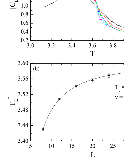
Figure 1: (color online) (a) Specific-heat curves as a function of the temperature. (b) Shift of the corresponding pseudocritical temperatures obtained from panel (a) where the specific heat attains its maximum.

The shift behavior of these finite-size anomalies $[Z]^{\ast}$ is used for the estimation of critical temperatures and the correlation length exponent by applying the standard fitting formula for second-order phase transitions

$$T_{L}^{\ast}=T_{\rm c}+bL^{-1/\nu}.$$ (8)

For the present study we have used two different order parameters: (i) the usual magnetization $M$, which is appropriate for describing transitions that involve the ferromagnetic phase, defined as

$$M=\frac{1}{N}\sum_{i=1}^{N}s_{i},$$ (9)

where $s_{i}$ is the spin variable and $N$ the number of lattice sites and (ii) the spin-glass overlap order parameter $q$, appropriate for the SG - P transition (also for the F - P transition), defined respectively as

$$q=\frac{1}{N}\sum_{i=1}^{N}s_{i}^{\alpha}s_{i}^{\beta},$$ (10)

where $s_{i}$ denotes the spin of the site $i$ and $\{\alpha,\beta\}$ represent two replicas of the same disorder realization. For the disordered system the corresponding, averaged over disorder, order parameter is obtained from the thermal averages of Eqs. (9) and (10).

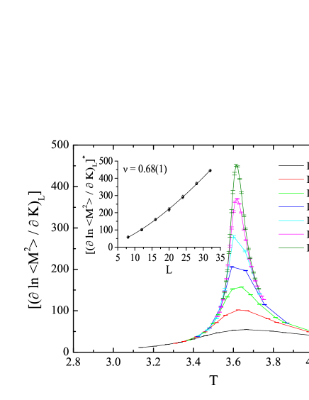
Figure 2: (color online) Temperature dependence of the second moment of the logarithmic derivative of the order parameter with respect to the inverse temperature (main panel) and the corresponding FSS behavior of the peaks (inset).

Following common practice FG_1 ; Hase10 ; hartmann_sggs ; balle_sg ; JankeBook ; katz_pg , we use a definition for the Binder cumulant LandBind00 of $Z$ ($M$ or $q$), based on the disorder averaged moments

$$U_{Z}=1-\frac{[\langle Z^{4}\rangle]}{3[\langle Z^{2}\rangle]^{2}}.$$ (11)

The crossings of the order-parameter’s fourth-order Binder cumulant $U_{M}$ or $U_{q}$ have been used as an alternative method in estimating the phase-diagram points. Furthermore, another route that provide us with complementary estimates of both the critical temperature and the exponent $\nu$ is that of data collapse LandBind00 . The application of this method is carried out assuming a scaling hypothesis of the form

$$U_{Z}\approx f[(T-T_{c})L^{1/\nu},$$ (12)

with $Z$ the above described order parameters. For the fitting procedure we have used autoScale, a program that performs a FSS analysis for given sets of simulated data collapse . The program implements the above scaling assumption which is expected to hold best close to the critical point and optimizes an initial set of scaling parameters that enforce a data collapse of the different sets. The optimum data collapse, achieved by the minimization procedure of the scaling parameters via the downhill simplex algorithm, is carried out by finding a fair compromise between a (rather small) value of a $\chi^{2}$/dof-like quantity and a reasonably large interval on the re-scaled abscissa.

III.2 Ferromagnetic - Paramagnetic Transition

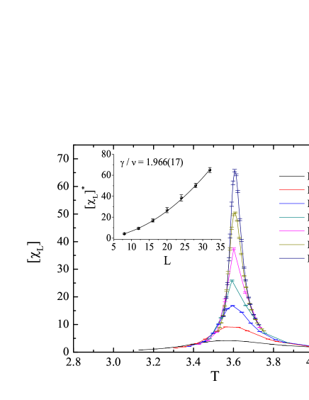
Figure 3: (color online) Illustration of the magnetic susceptibility as a function of the temperature (main panel) and the FSS of the peaks (inset).

Our main interest is the identification of the universality class of the model and this is, in general, characterized mainly from the critical exponent $\nu$ of the correlation length. Thus, we shall focus our analysis on the estimation of this exponent. Additional tests will include the estimation of the critical temperature via various FSS schemes, reflecting also the accuracy of our numerical data, as well as the estimation of the magnetic exponent ratio $\gamma/\nu$.

We start our analysis with Fig. 1, illustrating the scaling behavior of the specific heat. In particular, the upper panel (a) of this figure illustrates the specific-heat curves $[C_{L}]$ as a function of the temperature for the complete set of system sizes studied. The observed shift behavior of the specific-heat peaks is quantified in the corresponding lower panel (b), where we study the FSS of the relevant pseudocritical temperatures $T_{L}^{\ast}$, i.e., the temperatures where the specific heat attains its maximum. Applying the standard fitting formula for second-order phase transitions (8) on the numerical data we get the estimates $T_{\rm c}=3.605(8)$ and $\nu=0.687(18)$ for the critical temperature and the correlation length’s exponent, respectively, the latter indicating that the model shares the random Ising universality class, for which accurate estimates are $\nu=0.6837(53)$ balles_rdi , $0.683(3)$ hasen_fp , and $0.6835(25)$ anis_2 .

A further verification of the value of the critical exponent $\nu$ is provided via the FSS analysis of the peaks of the logarithmic derivative of the power $n=2$ of the order parameter with respect to the inverse temperature $K=1/T$, as shown in Fig. 2. In particular, in the main panel of this figure we illustrate the temperature dependence of the second moment [Eq. (6)] for the whole spectrum of lattice sizes studied and in the corresponding inset the FSS of the peaks. These are expected to scale as Eq. (7) and the power-law fitting, shown by the solid line, provides an estimate $\nu=0.68(1)$ for the exponent, in agreement with the values given above.

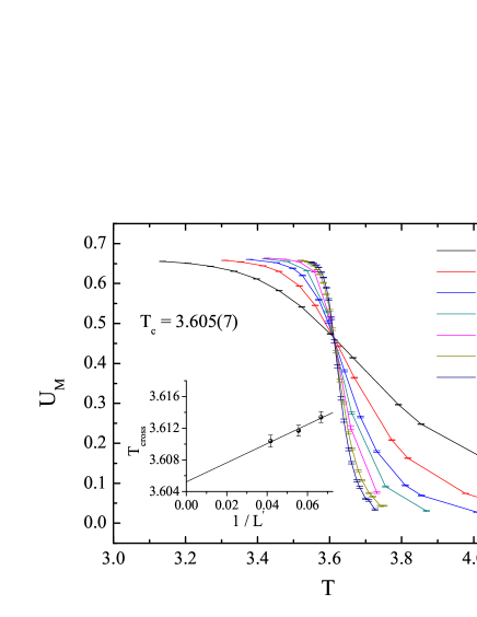
Figure 4: (color online) Crossings of the order-parameter’s fourth-order Binder cumulant (main panel) and infinite limit size extrapolation of the crossing points (inset).

We conclude our standard FSS analysis with the magnetic properties of the model, and in particular with the estimation of the magnetic exponent ratio $\gamma/\nu$ through the FSS of the magnetic susceptibility. In the main panel of Fig. 3 we present the temperature dependence of the magnetic susceptibility and the FSS of the corresponding peaks in the inset. The solid line shows a power-law fitting of the form (5) using the complete lattice-range spectrum. The outcome of the fitting provides an estimate $1.966(17)$ for the exponent ratio $\gamma/\nu$, in good agreement to the best-known literature estimates for the random Ising model which slightly vary around the value $1.965(6)$ balles_rdi ; berche-04 ; fytas-10 .

The above estimates are now further verified from a different approach, see Fig. 4, where the crossings of the order-parameter’s fourth-order Binder cumulant $U_{M}$ are illustrated. Although it is clear that the curves cross around the value $3.6$ which marks the location of the critical temperature of the system, a more refined analysis (see the inset) using the infinite-limit size extrapolation $L^{\prime}\rightarrow\infty$, where $L^{\prime}=1/(L_{1}+L_{2})$, of the crossing points $T_{\rm cross}$ of the pairs $(L_{1},\;L_{2})=(L,\;2L)$ gives an estimate of $T_{\rm c}=3.605(7)$ for the critical temperature.

Last but not least, we provide complementary estimates of both the critical temperature and the exponent $\nu$, via the method of data collapse collapse , as already discussed above in Sec.III.1. In the current case, the optimum data collapse for the order-parameter’s fourth-order Binder cumulant $U_{M}$ is shown in Fig. 5 and the resulting value for the critical temperature $T_{\rm c}=3.611(2)$ is in agreement with the previous estimates of Fig. 4 from the crossings of the same thermodynamic quantity. Additionally, the estimate $\nu=0.68(3)$ for the critical exponent of the correlation length is also in agreement with the previously obtained estimates.

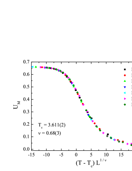
Figure 5: (color online) Collapse of the order-parameter’s fourth-order Binder cumulant of $M$.

Similar collapse attempt was performed for the Binder cumulant of the overlap order parameter $U_{q}$ and both critical estimates are presented in Table 1. Further cases for the lower part of the phase diagram, $p_{z}\in\{0.15,0.35,0.40\}$, were considered and the estimates are also in Table 1. For the values $p_{z}=0.425$ and $p_{z}=0.45$ we observe a considerable deviation in the estimated critical temperatures obtained from the corresponding collapse of $U_{M}$ and $U_{q}$, indicating that we are close to the multicritical point, in which the magnetization ceases to operate as the appropriate order parameter of the system. In particular, at $p_{z}=0.45$ we observe a significant deviation also in the estimate of the correlation length exponent. In this case the exponent produced from the collapse of the magnetization data is $1/\nu=0.86(12)$, whereas that produced from the overlap data is $1/\nu=0.67(12)$. The last value is close to $1/\nu=0.61(2)$ given by Hasenbusch et al. hasen_mcp , confirming that $p_{z}=0.45$ is close to the multicritical point.

III.3 Spin Glass - Paramagnetic Transition

From the closing remarks of the previous section it is expected that for the present model the multicritical point is close to $p_{z}=0.45$. The data for the F - SG transition line in Sec. III.4 are also in agreement with this estimate. Thus, two values $p_{z}=0.475$ and $p_{z}=0.5$ of our study belong to the SG - P transition line. For brevity we omit the details of our analysis for the first value, and we concentrate here only in the most interesting symmetric, $p_{z}=0.5$, case including a relevant ground-state study.

In the vicinity of the symmetric case $p_{z}=1/2$ at low enough temperatures, the presence of the spin-glass phase was clearly detected. The first indication was that the magnetization in this regime was not an appropriate order parameter (see also below the discussion for the $T=0$ magnetization order). Furthermore, at $p_{z}=0.475$ and $p_{z}=1/2$ (see Fig. 6), the data collapse analysis of $U_{q}$ produced critical exponent values $\nu=2.370(14)$ and $2.381(8)$ respectively, which are compatible to the estimated values of the SG - P transition found in the literature, namely the values $2.72(8)$ campb_sg , $2.15(15)$ balle_sg , $2.22(15)$ jorg , and the recent estimates $2.45(15)$ hasen_sg and $2.39(5)$ katz_pg . Similar results were also found in our recent study of the anisotropic case $\{p_{xy}\leq 0.4;p_{z}=0\}$, where $\nu$ was estimated $2.424(14)$ anis_2 .

The collapse of the Binder’s cumulant of the overlap order parameter, illustrated in the main panel of Fig. 6, gives an estimate of the order of $T_{\rm c}=1.77(8)$ for the critical temperature. We have also performed a linear extrapolation of the crossings points of $U_{q}$, as illustrated in the inset of this figure. The fit is performed in $1/L^{\prime}$, with $L^{\prime}=\{\frac{(L_{8}+L_{10})}{2},\frac{(L_{12}+L_{14})}{2},\frac{(L_{14}+L_{16})}{2}\}$. The resulting estimate is now $T_{\rm c}=1.68(12)$ in accordance with the value produced by the data collapse method. Therefore, the critical temperature of the longitudinal anisotropic model (denoted by $T_{B_{xy}}$) for the symmetric case is estimated to be considerably higher from the corresponding critical temperature of the isotropic model. Let us recall that the critical temperature of the isotropic model, denoted here by $T_{B}$, is of the order of $T_{B}=1.109(10)$ hasen_sg , and the corresponding temperature for the transverse anisotropic model $\{p_{xy}\leq 1/2;p_{z}=0\}$, denoted here by $T_{B_{z}}$, was estimated in the same range $T_{B_{z}}=1.111(25)$ anis_2 . The striking coincidence of points B and B_z, was further supported by the detailed ground-state study of Ref. PT1 .

In relevance to the above discussion, we now present in Fig. 7 the finite-size behavior of the ground-state energy per site($e_{\rm GS}=E_{\rm GS}/N$) for both anisotropic versions of our studies together with the known behavior of the isotropic $d=3$ EA model. Evidently, the clear difference in the limiting value of $e_{\rm GS}$ reflects the considerably higher critical temperature of the longitudinal anisotropic model. The known asymptotic estimations for the isotropic model are $e_{\rm GS}(L\rightarrow\infty)=-1.7863(4)$ pal96 , and $-1.7876(3)$ hart97 , and the second value is indicated by the dashed line in Fig. 7. For the present longitudinal anisotropic model the dashed line indicates the estimate $e_{\rm GS}(L\rightarrow\infty)=-2.0533(8)$. In the second part of this figure, we also show the size-decline of the $T=0$ magnetization order in the bulk $m=[\langle|M|\rangle]$. In the same figure an alternative order parameter is used based on the magnetization of the $xy$ planes, defined as $m_{\rm plane}=[\langle\sum_{\rm planes}|M_{\rm plane}|\rangle]$. Apparently, this pseudo-ordering (more pronounced for $m_{\rm plane}$) is only a finite-size effect that keeps also the ground-state energy in much lower values. The data shown in Fig. 7 were obtained via the PT algorithm using a practise analogous to that detailed in Ref. PT1 . The ensemble of disorder realizations varied from $15\times 10^{3}$ for $L=6$ to $100$ for $L=20$.

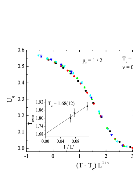
Figure 6: Critical temperature at the symmetry axis $p_{z}=1/2$. The collapse of the overlaps’s fourth-order Binder cumulant with the method outlined in Sec. III gives $T_{\rm c}=1.77(8)$, while the infinite-limit size extrapolation of $U_{q}$ crossings, illustrated in the inset, gives $T_{\rm c}=1.68(12)$. Details are provided in Sec. IV

.

We will now try to give an intuitive explanation of the above observations concerning the critical temperatures at the symmetric cases of the above spin-glass models. We suggest that, at these symmetry points - $p=p_{xy}=p_{z}=1/2$ - the critical temperatures $T_{B}$, $T_{B_{z}}$, and $T_{B_{xy}}$, are determined by some simple global frustration features of the models. First, let us assume that the coincidence of $T_{B}$ and $T_{B_{z}}$ observed in our earlier papers anis_2 ; PT1 is due to the fact that the density of the elementary squares of the lattice, denoted by $f$, which cannot simultaneously satisfy all their bonds (frustrated elementary squares or plaquette) is equal to $f=1/2$ for both models. This is also a plausible explanation of the apparent match in their ground-state energy found in Ref. PT1 (see also Fig. 7). For the current model, at the point $p_{z}=1/2$, the corresponding density is $f=1/3$, giving a lesser amount of frustration, thus producing a much higher $T_{\rm c}$, according to the above hypothesis.

Further global frustration features of the models can be invoked in order to support the above argument. As an example, let us consider the class of completely unfrustrated bonds. These type of bonds ($B_{0}$) on the simple cubic lattice have zero frustrated plaquette attached to them and one can define the corresponding densities $r({B_{0}})$ as fractions of the total number of bonds. Then, it is again easily seen that for both the isotropic model at $p=1/2$ and also for the transverse anisotropic model $\{p_{xy}=1/2;p_{z}=0\}$, $r({B_{0}})=(1/2)^{4}=0.0625$, whereas for the longitudinal anisotropic model this fraction is $r({B_{0}})=[2(1/2)^{4}+(1/2)^{2}]/3=1/6=0.166\cdots$. Thus, the longitudinal anisotropic model carries weaker frustration features, leading to higher critical temperature. Similar arguments can be applied for all five classes of bonds, i.e, $B_{0}$, $B_{1}$, $B_{2}$, $B_{3}$, and $B_{4}$ on the simple cubic lattice or their combinations, strengthening the hypothesis that $T_{\rm c}$ is mainly determined by simple global frustration features of the models.

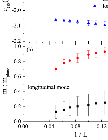
Figure 7: (a) Behavior of ground-state energies per site $e_{\rm GS}$ for the $d=3$ EA model and the two anisotropic versions. (b) Size-decline of the $T=0$ magnetization order in the bulk and $xy$-planes of the present longitudinal anisotropic model. In both panels error bars denote sample-to-sample fluctuations.

III.4 Ferromagnetic - Spin Glass Transition

The F - SG is the least investigated of the transition lines. A recent comprehensive FSS analysis for the isotropic EA model was performed by Ceccarelli et al. FG_1 . These authors found a new universality class by determining two points of the F - SG line corresponding to the temperatures $T=0.5$ and $T=1$. These two phase-diagram points, when compared to previous literature estimates for the multicritical and the $T=0$ F - SG critical point, clearly supported the earlier proposed reentrant behavior of the line. The extensive simulations of Ref. FG_1 involved lattice sizes within the range $L=4-20$, using many thousands of disorder realizations, even for $L=20$.

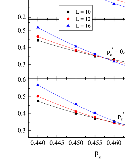
Figure 8: Illustration of the crossing behavior of the magnetization’s fourth-order Binder’s cumulant versus $p_{z}$ for the linear sizes $L=10$, $12$, and $L=16$ for three relevant temperatures outlined. The resulting F - SG transition line appears to be forward, according to the finite-size approximation shown.

Our attempt here to estimate the F - SG line for the present anisotropic EA model is not as extensive, we considered lattice sizes $L=10$, $12$, and $L=16$, with $8000$, $3000$, and $2000$ samples, respectively. The simulations were carried out for several values of $p_{z}$, close to the multicritical value $0.45$. Figure 8 illustrates the behavior of the fourth-order Binder’s cumulant of the magnetization $U_{M}$. The temperature sequence for each $p_{z}$ case went well deep into the paramagnetic phase ($T>2.6$) in order to avoid entrapment and ensure equilibration. While in most cases the minimum temperature was $T=1.5$, a very low temperature, namely $T=0.45$, was used in some production runs in order to record ground-state properties.

At $T=2.6$ in the range $p_{z}=0.44-0.47$ for linear sizes $L=10$ and $12$, $U_{M}$ does not show crossing and goes to zero as the size increases, indicating that we are in the paramagnetic region. Below the phase-diagram boundary we find crossing points as illustrated in Fig. 8 for three temperatures, namely $T=1.5$, $2$, and $T=2.35$, corresponding to crossing probabilities $p_{z}=0.4619(87)$, $0.4572(8)$, and $p_{z}=0.4513(35)$, respectively. The above were determined by the mean value of the crossings of the lines produced by second order polynomial fittings on the simulated points. Note that these values are rough estimates of the asymptotic results, since no extrapolation has been attempted. The F - SG transition line appears, at least according to the present finite-size approximation, to be forward and not reentrant, as shown for the isotropic model by Ceccarelli et al. FG_1 .

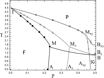
Figure 9: Global phase diagrams. Transition lines separate ferromagnetic (F), spin glass (SG), and paramagnetic (P) phases, and the multicritical points are denoted by M. Solid lines and full symbols illustrate the phase diagram of the isotropic EA model. F - P line points are taken from Ref. hasen_fp , the multicritical point M from Ref. hasen_mcp , the zero-temperature F - SG point A from Ref. hartmann_sggs , and the symmetric SG - P point B from Ref. hasen_sg . The dotted lines and open symbols correspond to the transverse anisotropic model $\{p_{z}=0;p_{xy}\leq 1/2\}$ described in detail in Ref. anis_2 . Finally the dashed lines and open symbols correspond to the present longitudinal anisotropic model $\{p_{z}\leq 1/2;p_{xy}=0\}$.

From the above discussion, the F - SG transition line for the present longitudinal anisotropic model appears to be forward, although an uncertainty remains because of the rather limited finite-size data at hand. However, the shifts of the crossings introduced by adding $L=16$ reinforces our claim. This behavior, if verified, could indicate to a link between frustration and the slope of the transition lines, since the present model has quite different frustration features close to the multicritical point. Thus, a need for a more extensive FSS analysis in this regime remains.

By using two estimates for the phase diagram, close to the multicritical point for the F - P line and the above three estimates of the F - SG transition line we find, using linear fittings, $p_{z}=0.4509(5)$ and $T=2.42(3)$ for the multicritical point. The $T=0$ F - SG critical point found by the linear fittings based on the above three estimates is $p_{z}=0.48(1)$, which is not far from the value obtained by a collapse of $U_{M}$ performed on our restricted ground-state data ($p_{z}=0.47(14)$). These estimates indicate a clear forward behavior.

Concluding the above discussion, it is also useful to recall that a forward ferromagnetic spin-glass line has been illustrated for a transverse anisotropic model with ratio of interactions $J^{z}/J^{xy}=0.5$ (see upper right panel of Fig.3 in Ref. anis_1 ). For the same ratio of interactions, the authors of Re. anis_1 also reported a very narrow spin-glass phase for the longitudinal anisotropic version of the model without commenting on the forward or reentrant character of this line (see the lower left panel of Fig.3 in Ref. anis_1 ). The origin of these findings, including those of the present paper, is not diaphanous and this makes the problem even more interesting.

IV Phase diagram and summary of estimates

In this Section we present the global phase diagrams of the following spin models: the well-known isotropic EA spin-glass model ea-model ; BindY86 ; hasen_fp , the transverse anisotropic case $\{p_{z}=0;p_{xy}\leq 1/2\}$ presented in our previous work anis_2 , and finally the present longitudinal anisotropic model $\{p_{z}\leq 1/2;p_{xy}=0\}$. The three models are symmetric around the $p$-, $p_{xy}$-, and $p_{z}=1/2$-axis respectively, thus the $p,p_{xy},p_{z}>1/2$ parts of the diagrams are omitted. The phase diagrams are illustrated in Fig. 9. Point I, is the well studied pure Ising model with $T_{\rm c}=4.5115232(16)$ Hase10 ; camp_is ; guida_is ; Butera-02 ; deng_is ; blote_is . The full star at $p=0.117(3)$ in the F - P line denotes the improved model proposed in Ref. hasen_fp , where scaling corrections are minimum. Open and half full stars represent respectively points of the transverse anisotropic model $p_{xy}=0.176$ anis_2 and $p_{z}=0.25$ of the present longitudinal anisotropic model. Note that, the $x$-axis labelled as $p$, represents the probability $p$ for the isotropic model, $p_{xy}$ for the transverse anisotropic model, and $p_{z}$ for the present longitudinal anisotropic model. Further details are given in the caption of Fig. 9.

The phase diagrams of the isotropic and transverse anisotropic models were discussed in Refs. anis_2 ; PT1 , where the most striking feature of the coincidence of points B and B_z, was supported by the detailed ground-state study of Ref. PT1 . As seen now from Fig. 9, the present model yields a SG - P point B_xy at a significantly higher temperature and the origin of this phenomenon we believe stems from the different frustration features, already discussed in Sec. III.3.

Table 1: Summary of estimates for the critical temperature and the critical exponent $\nu$ obtained for all the values of $p_{z}$ studied. For $p_{z}\leq 0.45$ two sets of results are given, obtained from the data collapse method as discussed in the main text, corresponding to the order-parameter’s $U_{M}$ (second and third column) and overlap’s $U_{q}$ (fourth and fifth) fourth-order Binder cumulant. For $p_{z}>0.45$, estimates only via the collapse of $U_{q}$ are given.

	$U_{M}$		$U_{q}$
$p_{z}$	$T_{\rm c}$	$1/\nu$	$T_{\rm c}$	$1/\nu$
0.15	3.993(2)	1.465(9)	3.995(2)	1.46(2)
0.25	3.611(2)	1.464(12)	3.6128(9)	1.46(4)
0.35	3.172(2)	1.43(9)	3.166(9)	1.46(4)
0.4	2.90(2)	1.46(21)	2.880(12)	1.47(12)
0.425	2.74(3)	1.46(42)	2.705(33)	1.46(5)
0.45	2.41(12)	0.86(12)	2.43(5)	0.67(12)
0.475			2.00(15)	0.42(8)
0.5			1.77(8)	0.42(5)

V Discussion and concluding remarks

In the present manuscript, we presented the phase diagram and critical behavior of a further anisotropic case of the $\pm J$ three-dimensional Ising model on the simple cubic lattice. The current spatially anisotropic $\pm J$ bond randomness was applied only in the $z$ direction, whereas in the other two directions, $xy$ - planes, a ferromagnetic exchange was implemented. The phase diagram of the model under study was compared to that of the corresponding isotropic one, as well as to the phase diagram of the anisotropic case in which the $\pm J$ bond randomness was applied only in the $xy$ - planes. The observed differences in the global phase diagrams were critically discussed, assuming that some global frustration features of the models determine the critical temperature, especially at the symmetry points of the models. As we have shown, the differences in frustration features, at the symmetry point, give rise in the present model to a considerable increase of the transition temperature. Furthermore, our data for the ferromagnetic - spin glass transition line are supporting a forward behavior in contrast to the reentrant behavior of the isotropic model, and this is also proposed as an effect of the frustration features of the model.

Our scaling analysis verified, once more, the interesting feature of the irrelevance for the critical behavior of the spatial anisotropy. This aspect of universality was also found in the renormalization-group study of Ref. anis_1 . The signs of this universality can be directly identified by simply comparing our critical estimates shown in Table 1 to those of the relevant literature. It is natural to expect that the general universality, observed among these models, is a reflection of the spatially stochastic character of the quenched disorder and the frustration, although the differences in some global characteristics may produce very interesting changes in the corresponding phase diagrams. It will be useful, as a feature task, to further understand the effects of the global frustration features on both phase diagrams and also on the critical behavior of these simple spin-glass models. Research in this direction is currently under way.

- (1) S.F. Edwards and P.W. Anderson, J. Phys. F: Metal Physics 5, 965 (1975).
- (2) K. Binder and A.P. Young, Rev. Mod. Phys. 58, 801 (1986).
- (3) C. Güven, A.N. Berker, M. Hinczewski, and H. Nishimori, Phys. Rev. E 77, 061110 (2008).
- (4) T. Papakonstantinou and A. Malakis, Phys. Rev. E 87, 012132 (2013).
- (5) G. Ceccarelli, A. Pelissetto, and E. Vicari, Phys. Rev. B 84, 134202 (2011).
- (6) M. Hasenbusch, F. Parisen Toldin, A. Pelissetto, and E. Vicari, Phys. Rev. B 76, 094402 (2007).
- (7) M. Hasenbusch, A. Pelissetto, and E. Vicari, Phys. Rev. B 78, 214205 (2008).
- (8) H.G. Katzgraber, M. Körner, and A.P. Young, Phys. Rev. B 73, 224432 (2006).
- (9) T. Jörg, Phys. Rev. B 73, 224431 (2006).
- (10) I.A. Campbell, K. Hukushima, and H. Takayama, Phys. Rev. B 76, 134421 (2007).
- (11) H.G. Ballesteros, A. Cruz, L.A. Fernández, V. Martín-Mayor, J. Pech, J.J. Ruiz-Lorenzo, A. Tarancón, P. Téllez, C.L. Ullod, and C. Ungil, Phys. Rev. B 62, 14237 (2000).
- (12) M. Palassini and S. Caracciolo, Phys. Rev. Lett. 82, 5128 (1999).
- (13) N. Kawashima and H. Rieger, arXiv:cond-mat/0312432.
- (14) A. Billoire, L.A. Fernández, A. Maiorano, E. Marinari, V. Martín-Mayor, and D. Yllanes, J. Stat. Mech.: Theory Exp. (2011) P10019.
- (15) M. Hasenbusch, F. Parisen Toldin, A. Pelissetto, and E. Vicari, Phys. Rev. B 76, 184202 (2007).
- (16) Y. Ozeki and H. Nishimori, J. Phy. Soc. Jpn. 56, 3265 (1987).
- (17) Y. Ozeki and N. Ito, J. Phys. A: Math. Gen. 31, 5451 (1998).
- (18) R.R.P. Singh, Phys. Rev. Lett. 67, 899 (1991).
- (19) P.L. Doussal and A.B. Harris, Phys. Rev. Lett. 61, 625 (1988).
- (20) P.L. Doussal and A.B. Harris, Phys. Rev. B 40, 9249 (1989).
- (21) H. Nishimori, Statistical Physics of Spin Glasses and Information Processing: An Introduction (Oxford University Press, USA, 2001).
- (22) H. Nishimori, J. Phys. C: Solid State Phys. 13, 4071 (1980).
- (23) H. Nishimori, Prog. Theor. Phys. 66, 1169 (1981).
- (24) H. Nishimori, J. Phys. Soc. Jpn. 55, 3305 (1986).
- (25) A. Malakis and T. Papakonstantinou, Phys. Rev. E 88, 013312 (2013).
- (26) T. Papakonstantinou and A. Malakis, J. Phys.: Conf. Ser. 487, 012010 (2014).
- (27) R.H. Swendsen and J.-S. Wang, Phys. Rev. Lett. 57, 2607 (1986).
- (28) K. Hukushima and K. Nemoto, J. Phys. Soc. Jpn. 65, 1604 (1996).
- (29) E. Marinari, G. Parisi, and J.J. Ruiz-Lorenzo, in Spin Glasses and Random Fields, edited by A.P. Young (World Scientific, Singapore,1998), p.59.
- (30) M.E.J Newman and G.T. Barkema, Monte Carlo Methods in Statistical Physics (Clarendon, Oxford, 1999).
- (31) N. Metropolis, A.W. Rosenbluth, M.N. Rosenbluth, A.H. Teller, and E. Teller, J. Chem. Phys. 21, 1087 (1953).
- (32) E. Bittner, Andreas Nußbaumer, and W. Janke, Phys. Rev. Lett. 101, 130603 (2008).
- (33) Y. Sugita and Y. Okamoto, Chem. Phys. Lett. 314, 141 (1999).
- (34) E. Bittner and W. Janke, Phys. Rev. E 84, 036701 (2011).
- (35) D.J. Earl and M.W. Deem, Phys. Chem. Chem. Phys., 7, 3910 (2005).
- (36) R.H. Swendsen and J.S. Wang, Phys. Rev. Lett. 58, 86 (1987); U. Wolff, ibid. 62, 361 (1989).
- (37) D.P. Landau and K. Binder, Monte Carlo Simulations in Statistical Physics (Cambridge University Press, Cambridge, 2000).
- (38) A. Malakis, A.N. Berker, N.G. Fytas, and T. Papakonstantinou, Phys. Rev. E 85, 061106 (2012).
- (39) A.M. Ferrenberg and D.P. Landau, Phys. Rev. B 44, 5081 (1991).
- (40) O. Melchert, arXiv:0910.5403.
- (41) H.G. Ballesteros, L.A. Fernández, V. Martín-Mayor, A. Muñoz Sudupe, G. Parisi, and J.J. Ruiz-Lorenzo, Phys. Rev. B 58, 2740 (1998).
- (42) M. Hasenbusch, F. Parisen Toldin, A. Pelissetto, and E. Vicari, J. Stat. Mech.: Theory Exp. (2007) P02016.
- (43) A. Pelissetto and E. Vicari, Phys. Rev. B 62, 6393 (2000).
- (44) P.E. Berche, C. Chatelain, B. Berche, and W. Janke, Eur. Phys. J. B 38, 463 (2004).
- (45) N.G. Fytas and P.E. Theodorakis, Phys. Rev. E 82, 062101 (2010); P.E. Theodorakis and N.G. Fytas, Eur. Phys. J. B 81, 245 (2011).
- (46) K.F. Pal, Physica A 223, 283 (1996).
- (47) A.K. Hartmann, Europhys. Lett. 40, 429 (1997).
- (48) M. Hasenbusch, Phys. Rev. B 82, 174433 (2010).
- (49) M. Campostrini, A. Pelissetto, P. Rossi, and E. Vicari, Phys. Rev. E 65, 066127 (2002).
- (50) R. Guida and J. Zinn-Justin, J. Phys. A: Math. Gen. 31, 8103 (1998).
- (51) P. Butera and M. Comi, Phys. Rev. B 65, 144431 (2002).
- (52) Y. Deng and H.W.J. Blöte, Phys. Rev. E 68, 036125 (2003).
- (53) H.W.J. Blöte, E. Luijten, and J.R. Heringa, J. Phys. A: Math. Gen. 28, 6289 (1995).
- (54) A.K. Hartmann, Phys. Rev. B 59, 3617 (1999).
- (55) W. Janke. Monte Carlo Methods in Classical Statistical Physics (Springer Berlin Heidelberg, 2008)