A Multidomain Model for Ionic Electrodiffusion and Osmosis with an Application to Cortical Spreading Depression

Abstract

Ionic electrodiffusion and osmotic water flow are central processes in many physiological systems. We formulate a system of partial differential equations that governs ion movement and water flow in biological tissue. A salient feature of this model is that it satisfies a free energy identity, ensuring the thermodynamic consistency of the model. A numerical scheme is developed for the model in one spatial dimension and is applied to a model of cortical spreading depression, a propagating breakdown of ionic and cell volume homeostasis in the brain.

1 Introduction

In this paper, we formulate a system of partial differential equations (PDE) that governs ionic electrodiffusion and osmotic water flow, to study tissue-level physiological phenomena. To demonstrate the use of the model, we apply this to the study of cortical spreading depression, a pathological phenomenon of the brain that is linked to migraine aura and other diseases.

We now describe our modeling approach. Biological tissue can often be seen as composed of multiple interpenetrating compartments. Cardiac tissue, for example, can be seen as composed of two interpenetrating compartments, the space that consists of interconnected cardiomyocytes and the extracellular space. The number of compartments may not be restricted to two. In the central nervous system, one may consider the neuronal, glial and extracellular compartments. In studying physiological phenomena at the tissue level, it is often impractical to use models with exquisite cellular detail. If the spatial variations in the biophysical variables of interest are slow compared to the cellular spatial scale, we may model the system instead as a homogenized continuum. The first such model, the bidomain model, was introduced in [16, 17, 56], and its application to cardiac electrophysiology [22] is probably the most important and successful example of this coarse-grained approach in physiology. Let us use the cardiac bidomain model to further to illustrate this approach. The main variables of interest in cardiac electrophysiology are the intracellular and extracellular potentials, $\phi_{i}(\mathbf{x})$ and $\phi_{e}(\mathbf{x})$ where $\mathbf{x}$ is the spatial coordinate. From a microscopic standpoint, these values should only be defined within their respective compartments. At the coarse-grained level, however, we take the view that it is impossible to distinguish whether a given spatial point is inside the cell or outside the cell. The intracellular and extracellular potentials are now defined everywhere and cardiac tissue is thus seen as an biphasic continuum. In this paper, we shall call such models multidomain models to emphasize the fact that the formalism is not restricted to just two interpenetrating phases. We note that such coarse-grained models are also widely used in the material sciences to describe, for example, multiphase flow [14].

Our goal is to formulate a multidomain model that describes ionic electrodiffusion and osmosis. This can be seen as a generalization of the cardiac bidomain model, which only treats electrical current flow. Ionic electrodiffusion and osmosis have been modeled to varying degrees of detail in different physiological systems. These include the kidney [59], gastric mucosa [33], cerebral edema and hydrocephalus [11], cartilage [20, 21], and the lens [34] and cornea [32] of the eye. Here, we develop a time-dependent PDE model that fully incorporates both ionic electrodiffusion and osmotic water flow in multiphasic tissue. Ion balance is governed by the Nernst-Planck electrodiffusion equations with source terms describing transmembrane ion flux. For water balance, we have the usual continuity equations with source terms describing transmembrane water flow. An important feature that distinguishes our model from previous models is that it satisfies a free energy identity, which ensures that electrodiffusive and osmotic effects are treated in a thermodynamically consistent fashion. The use of free energy identities as a guiding principle in formulating equations originates in the work of Onsager [46], and this approach has been widely adopted in soft condensed matter physics [9, 10, 25, 15]. The present work is closely related to our recent work in [37, 39, 41, 6], wherein the free energy identity played an essential role in ionic electrodiffusion problems arising in physiology and the material sciences. One practical benefit of the physically consistent formulation of our model is that it treats fast cable (or electrotonic/electrical current) effects and the much slower effects mediated by ion concentration gradients in a single unified framework. This is significant especially in the context of ion homeostasis in the brain, in which these fast and slow effects are both important and tightly coupled.

To demonstrate the use of the model (and to test our computational scheme), we have included a preliminary modeling study of cortical spreading depression (SD). SD is a pathological phenomenon of the central nervous system, first reported 70 years ago [31]. Neurons sustain a complete depolarization and loss of functions for seconds to minutes. A massive redistribution of ions takes place [18] resulting in extracellular potassium concentrations in excess of $50$mmol/l. Also seen is neuronal swelling and narrowing of the extracellular space. This breakdown in ionic and volume homeostasis spreads across gray matter at speeds of $2-7$mm/min. SD is the physiological substrate of migraine aura, and it is also related to other brain pathologies such as stroke, seizures and trauma [13]. Studying SD is important, not only because of its close relationship with important diseases but also because a good understanding of SD will lead to a better understanding of brain ionic homeostasis, and hence of the workings of the central nervous system. Despite intensive research efforts, basic questions about SD remain unanswered [36, 23]. We refer the reader to [53, 35, 52, 5, 8] for reviews on SD.

There have been many modeling studies on SD propagation [19, 49, 54, 55, 44, 48, 50, 51, 1, 2, 7, 60, 4], most of which are of reaction-diffusion type. The large excursions in ionic concentration necessitates incorporation of ionic electrodiffusion and osmotic effects, and our model is well-suited for this application. As a natural output of our model, we can compute the negative shift in the extracellular potential (negative DC shift), an important experimental signal of SD. To the best of our knowledge, this is the first successful computation of this quantity. We then examine the effect of gap junctional coupling and extracellular chloride concentration on SD propagation speed. In particular, we argue that gap junctional coupling is unlikely to play an important role in SD propagation [51].

The paper is organized as follows. In Section 2 we formulate the model. In Section 3, we discuss the free energy identity. This identity allows us to place thermodynamic restrictions on the constitutive laws for the transmembrane fluxes. In Section 4, we make the equations dimensionless and discuss model reduction when certain dimensionless quantities are taken to $0$. In particular, we clarify the relationship between our multidomain electrodiffusion model with the cardiac bidomain model. In Section 5, we discuss the numerical discretization of our system. We devise a implicit numerical method that preserves ionic concentrations and satisfies a discrete free energy inequality. In Section 6, we perform simulations of SD. Appendix A describes some of the details of the SD model and simulation and Appendix B includes some remarks on the computation of the extracellular voltage.

2 Model Formulation

We suppose that the tissue of interest occupies a smooth bounded region $\Omega\in\mathbb{R}^{3}$. As discussed in the Introduction, we view biological tissue as being a multiphasic continuum. Suppose the tissue is composed of $N$ interpenetrating compartments which we label by $k$. We assume that $k=N$ corresponds to the extracellular space and that all other compartments communicate with the extracellular space only. When we only consider the intracellular and extracellular spaces, $N=2$ and the $2$nd compartment will be the extracellular space. In the central nervous system, we may consider neuronal, glial and extracellular spaces and the extracellular space corresponding to the $3$rd compartment, and the other two compartments communicating with the extracellular compartment. To each point in space, we assign a volume fraction $\alpha_{k}$ for each compartment. By definition, we have:

$$\sum_{k=1}^{N}\alpha_{k}(\mathbf{x},t)=1.$$ (2.1)

Note that $\alpha_{k}$ is a function of space and time.

In the following we shall introduce several parameters that may be influenced by the microscopic geometric details of the tissue. Mechanical properties of cells and hydraulic conductivity are examples of such parameters. We shall make the assumption that these parameters depend on the underlying microscopic geometry only through its influence on $\alpha_{k}$.

In order to describe the time evolution of $\alpha_{k}$, we introduce the water flow velocity field $\mathbf{u}_{k}$ defined for each compartment. The volume fraction $\alpha_{k}$ satisfies the following equation:

$$\frac{\partial\alpha_{k}}{\partial t}+\nabla\cdot(\alpha_{k}\mathbf{u}_{k}) =-\gamma_{k}w_{k},\;k=1,\cdots,N-1$$ (2.2)

$$\frac{\partial\alpha_{N}}{\partial t}+\nabla\cdot(\alpha_{N}\mathbf{u}_{N}) =\sum_{k=1}^{N-1}\gamma_{k}w_{k}$$ (2.3)

The coefficient $\gamma_{k}$ represents the area of cell membrane between compartment $k$ and the extracellular space per unit volume of tissue, and has units of $1/\text{length}$. We assume that the membrane does not stretch appreciably, and take $\gamma_{k}$ to be constant in time. Transmembrane water flow per unit area of membrane is given by $w_{k}$ where flux going from compartment $k$ into the extracellular space is taken positive. Transmembrane water flow $w_{k}$ is a function of the volume fractions $\alpha_{k}$ as well as the ionic concentrations, the compartmental pressures and possibly the compartmental voltages, biophysical variables to be introduced below. This constitutive relation for $w_{k}$ will be discussed further in Section 3. Equation (2.2) and (2.3), together with (2.1) yields:

$$\nabla\cdot\left(\sum_{k=1}^{N}\alpha_{k}\mathbf{u}_{k}\right)=0.$$ (2.4)

This condition states that the volume-fraction weighted velocity is divergence free, and corresponds to the incompressiblity condition for simple fluids.

We now turn to the dynamics of ionic concentrations. Let $c_{i}^{k}$ be the ionic concentration of the $i$-th species of ion in compartment $k$. We shall mainly be concerned with the inorganic ions (Na⁺, K⁺, Cl^- etc) that play an important role in electrophysiology and are major contributors to osmotic pressure. Among the ions we do not track explicitly are the organic ions, including soluble proteins and sugars and constituents of the intracellular and extracellular matrix. For simplicity, we neglect diffusion and transmembrane movement of these ions, which we call the immobile ions. As we shall see, the background ions will exert electrostatic effects and contribute to osmotic pressure. We shall keep track of $M$ species of mobile ion. For each ionic species $i=1,\cdots,M$, we have the following conservation equations in each compartment.

$$\frac{\partial(\alpha_{k}c_{i}^{k})}{\partial t} =-\nabla\cdot\mathbf{f}_{i}^{k}-\gamma_{k}g_{i}^{k},\;k=1,\cdots,N-1,$$ (2.5)

$$\frac{\partial(\alpha_{N}c_{i}^{N})}{\partial t} =-\nabla\cdot\mathbf{f}_{i}^{N}+\sum_{k=1}^{N-1}\gamma_{k}g_{i}^{k},$$ (2.6)

$$\mathbf{f}_{i}^{k} =-D_{i}^{k}\left(\nabla c_{i}^{k}+\frac{z_{i}Fc_{i}^{k}}{RT}\nabla\phi_{k}\right)+\alpha_{k}\mathbf{u}_{k}c_{i}^{k},\;k=1,\cdots,N.$$ (2.7)

In these equations, $F$ is the Faraday constant, $D_{i}^{k}$ is the diffusion coefficient, $z_{i}$ is the valence of the $i$-th species of ion, $RT$ is the ideal gas constant times absolute temperature, and $\phi^{k}$ is the electrostatic potential of the $k$-th compartment. The diffusion coefficient $D_{i}^{k}$ is in general a diffusion tensor that may be a function of $\alpha_{k}$. The terms $g_{i}^{k}$ in (2.5) and (2.6) are the transmembrane fluxes per unit membrane area for each species of ion. Biophysically, these are fluxes that flow through ion channels, transporters, or pumps that are located on the cell membrane. It is useful to split this transmembrane flux into two terms:

$$g_{i}^{k}=j_{i}^{k}+h_{i}^{k}.$$ (2.8)

The flux $j_{i}^{k}$ is the passive flux corresponding to ion channel and transporter fluxes. The flux $h_{i}^{k}$ is the active flux through ionic pumps. Both $j_{i}^{k}$ and $h_{i}^{k}$ are functions of the ionic concentrations, compartmental voltage, and possibly the volume fractions and the compartmental pressure. The compartmental pressure $p_{k}$ will be introduced shortly. Ion channel currents are often also controlled by channel gating, and in such cases, $j_{i}^{k}$ will also depend on gating variables. The constitutive relations for $j_{i}^{k}$ and $h_{i}^{k}$ will be discussed further in Section 3, where we give a precise definition of what is meant by a passive flux.

To specify the electrostatic potential $\phi^{k}$, we have the following equations which we call the charge capacitor relation:

$$\gamma_{k}C_{\rm m}^{k}\phi_{kN} =z_{0}^{k}Fa_{k}+\sum_{i=1}^{M}z_{i}F\alpha_{k}c_{i}^{k},\;\phi_{kN}=\phi_{k}-\phi_{N},\;k=1,\cdots,N-1,$$ (2.9)

$$-\sum_{k=1}^{N-1}\gamma_{k}C_{\rm m}^{k}\phi_{kN} =z_{0}^{N}Fa_{N}+\sum_{i=1}^{M}z_{i}F\alpha_{N}c_{i}^{N}$$ (2.10)

These equations state that excess charge is stored on the membrane capacitor. The constant $C_{\rm m}^{k}$ is the membrane capacitance per unit area of membrane separating the $k$-th and $N$-th compartment. The immobile charge density is given by $z_{0}^{k}Fa_{k}$ where $z_{0}^{k}$ and $a_{k}$ are the valence and amount of immobile solutes respectively. We assume that the $a_{k}$ are constant in time. Given the smallness of the capacitance, it is often an excellent approximation to use the following electroneutrality condition in place of (2.9) and (2.10):

$$z_{0}^{k}Fa_{k}+\sum_{i=1}^{M}z_{i}F\alpha_{k}c_{i}^{k}=0,\;k=1,\cdots,N.$$ (2.11)

We shall come back to this approximation when we discuss non-dimensionalization in Section 4. The charge capacitor relation can, thus, also be considered a condition for near electroneutrality. Under the electroneutrality approximation, $\phi_{k}$ is determined so that the electroneutrality condition is satisfied. A differential equation for $\phi_{k}$ may be obtained by taking the time derivative of (2.11) with respect to $t$ and using (2.5) and (2.6). We shall discuss this further later on.

We also point out that the charge capacitor relation of (2.9) and (2.10) plays the role of the Poisson equation in the Poisson-Nernst-Planck system, in that (2.9) and (2.10) determine the electrostatic potential. The use of this relationship in pump-leak model is standard [24, 29]. Its use in a spatially extended context appears in [47, 30]. We also point to [38, 40] in which similar relations are used. The use of the the charge capacitor relation in place of the Poisson equation is warranted in part because the space charge layer (Debye length, typically on the order of nanometers) is very small compared even to the cellular length scale. Indeed, much of the interest in applications of the Poisson-Nernst-Planck system in biology concerns modeling of ion channels and other biomolecules [45, 57], a problem at much smaller length scales than the problem at hand.

Let us turn to the equations for $\mathbf{u}_{k}$. We introduce the compartmental pressure fields $p_{k}$.

$$\zeta_{k}\mathbf{u}_{k}=-\nabla\widetilde{p}_{k}-\sum_{i=1}^{M}z_{i}Fc_{i}^{k}\nabla\phi_{k},\;\widetilde{p}_{k}=p_{k}-RT\frac{a_{k}}{\alpha_{k}},\;k=1\cdots N.$$ (2.12)

Here, $\zeta_{k}$ is the hydraulic resistivity for the $k$-th compartment and $a_{k}$ is the amount of immobile ions in the $k$-th compartment. The above states that the flow is driven by electrostatic forces and the modified pressure $\widetilde{p}_{k}$. The modified pressure $\widetilde{p}_{k}$ has a mechanical contribution $p_{k}$ as well as a contribution from the immobile ions $a_{k}/\alpha_{k}$. The $a_{k}/\alpha_{k}$ term is known as the oncotic pressure in the physiology literature [3]. The hydraulic resistivity $\zeta_{k}$ is in general a position dependent tensor, but we may, for simplicity, assume that $\zeta_{k}$ is a scalar. For the extracellular space, a simple prescription may be to set $\zeta_{k}$ proportional to $\alpha_{k}$. In the case of the intracellular space, hydraulic resistivity in many tissues should be controlled by gap junctions connecting adjacent cells. In the absence of gap junctions, $(\zeta_{k})^{-1}$ may be set to $0$.

To determine the compartmental pressures $p_{k}$, we consider force balance between compartment $k$ and the extracellular space. This leads to the following expression:

$$p_{k}-p_{N}=\tau_{k}(\alpha),\;k=1,\cdots,N-1$$ (2.13)

where $\tau_{k}$ is the mechanical tension per unit area of the membrane separating compartment $k$ and the extracellular space. The membrane tension $\tau_{k}$ should be determined by the instantaneous microscopic configuration of the membrane. Given our assumption that the effects of microscopic geometry manifests itself only through its influence on $\alpha$, $\tau_{k}$ must be given as a function of the volume fractions $\alpha=(\alpha_{1},\cdots,\alpha_{N})$. A simple constitutive relation may be:

$$\tau_{k}=S_{k}(\alpha_{k}-\alpha_{k}^{0})$$ (2.14)

where $\alpha_{k}^{0}$ is the volume fraction at which the membrane has no mechanical tension and $S_{k}$ is a stiffness constant. We consider a class of constitutive relations that can be derived from some energy function $\mathcal{E}(\alpha_{1},\cdots,\alpha_{N-1})$ in the following sense:

$$\tau_{k}(\alpha)=\frac{\partial\mathcal{E}}{\partial\alpha_{k}}.$$ (2.15)

The simple constitutive relation (2.14) clearly satisfies condition (2.15) with the choice:

$$\mathcal{E}=\frac{1}{2}\sum_{k=1}^{N-1}S_{k}(\alpha_{k}-\alpha_{k}^{0})^{2}.$$ (2.16)

We have only specified the constitutive relation for the difference $p_{k}-p_{N}$. The extracellular pressure $p_{N}$ is determined so that the incompressibility condition (2.4) is satisfied. We may derive an equation for $p_{N}$ by multiplying (2.12) by $\alpha_{k}(\zeta_{k})^{-1}$, taking the divergence and taking the summation in $k=1,\cdots,N$. We obtain:

$$0=\nabla\cdot\left(\sum_{k=1}^{N}\left(\alpha_{k}\zeta_{k}^{-1}\left(\nabla\left(\tau_{k}(\alpha)+p_{N}-\frac{RTa_{k}}{\alpha_{k}}\right)+\sum_{i=1}^{N}z_{i}Fc_{i}^{k}\nabla\phi_{k}\right)\right)\right),$$ (2.17)

where we set $\tau_{N}=0$ for notational convenience and used (2.4) to obtain $0$ on the left hand side of the above.

Boundary conditions will strongly depend on the problem in question. In this paper we shall assume no flux boundary conditions at the boundary $\partial\Omega$:

$$\mathbf{u}_{k}\cdot\mathbf{n}=0,\;\;\mathbf{f}_{i}^{k}\cdot\mathbf{n}=0$$ (2.18)

where $\mathbf{n}$ is the outward unit normal on $\partial\Omega$.

In the above, our region $\Omega$ was a bounded region in $\mathbb{R}^{3}$. It is also meaningful to consider the above equations in a one-dimensional or two-dimensional region. This corresponds to a problem in which the biophysical variables of interest are assumed to have no spatial dependence in two or one coordinate direction respectively. Most of the calculations to follow remain valid when $\Omega$ is a 1D or 2D region instead of a 3D region. In Section 5, we present a numerical simulation for a 1D version of the model.

3 A Free Energy Identity

We shall now state and prove a free energy identity for the above system of equations. Before we state the energy identity, we define some useful quantities.

$$\mu_{i}^{k} =RT(\ln c_{i}^{k}+1)+z_{i}Fc_{i}^{k}\phi_{k},$$ (3.1)

$$\pi_{{\rm w}k} =RT\left(\frac{a_{k}}{\alpha_{k}}+\sum_{i=1}^{M}c_{i}^{k}\right).$$ (3.2)

The quantity $\mu_{i}^{k}$ is the chemical potential of the $i$-th species of ion in the $k$-th compartment. The quantity $\pi_{{\rm w}k}$ is the osmotic pressure. It is also useful to define the following water potential:

$$\psi_{k}=p_{k}-\pi_{{\rm w}k}.$$ (3.3)

Theorem 1.

Suppose $\alpha_{k},\mathbf{u}_{k},c_{i}^{k},\phi_{k}$ and $p_{k}$ are smooth functions that satisfy (2.1), (2.2), (2.3), (2.5), (2.6), (2.9), (2.10), (2.12), (2.13), (2.15) and (2.18). Then, the following identity holds.

$$\begin{split}\frac{dG}{dt}&=-I_{\rm bulk}-I_{mem},\\ G&=\int_{\Omega}\left(\mathcal{E}+\sum_{k=1}^{N}\left(RT\left(a_{k}\ln\left(\frac{a_{k}}{\alpha_{k}}\right)+\sum_{i=1}^{M}\alpha_{k}c_{i}^{k}\ln c_{i}^{k}\right)\right)+\sum_{k=1}^{N-1}\frac{1}{2}\gamma_{k}C_{\rm m}\phi_{kN}^{2}\right)d\mathbf{x},\\ I_{\rm bulk}&=\int_{\Omega}\left(\sum_{k=1}^{N}\left(\alpha_{k}\zeta_{k}\left\lvert\mathbf{u}_{k}\right\rvert^{2}+\sum_{i=1}^{M}\frac{D_{i}^{k}c_{i}^{k}}{RT}\left\lvert\nabla\mu_{i}^{k}\right\rvert^{2}\right)\right)d\mathbf{x},\\ I_{\rm mem}&=\int_{\Omega}\left(\sum_{k=1}^{N-1}\gamma_{k}\left(\psi_{kN}w_{k}+\sum_{i=1}^{M}\mu_{i}^{kN}g_{i}^{k}\right)\right)d\mathbf{x},\end{split}$$ (3.4)

where $\psi_{kN}=\psi_{k}-\psi_{N}$ and $\mu_{i}^{kN}=\mu_{i}^{k}-\mu_{i}^{N}$.

In (3.4), the function $G$ should be interpreted as the free energy of the system, given as the sum of the elastic energy, the free energy from the ions and the electrical energy stored on the membrane capacitor. The change in $G$ is written as a sum of two parts, $-I_{\rm bulk}$, arising from biophysical processes within each compartment, and, $-I_{\rm mem}$, across the cell membranes.

Proof.

Multiply both sides of (2.5) by $\mu_{i}^{k}$ and integrate over $\Omega$. The left hand side yields:

$$\begin{split}\int_{\Omega}\mu_{i}^{k}\frac{\partial(\alpha_{k}c_{i}^{k})}{\partial t}d\mathbf{x}=\int_{\Omega}\left(RT\left(\frac{\partial}{\partial t}(\alpha_{k}c_{i}^{k}\ln c_{i}^{k})+c_{i}^{k}\frac{\partial\alpha_{k}}{\partial t}\right)+z_{k}F\phi_{k}\frac{\partial(\alpha_{k}c_{i}^{k})}{\partial t}\right)d\mathbf{x}\end{split}$$ (3.5)

The left hand side for (2.5) yields:

$$\begin{split}&-\int_{\Omega}\mu_{i}^{k}(\nabla\cdot\mathbf{f}_{i}^{k}+\gamma_{k}g_{i}^{k})d\mathbf{x}=\int_{\Omega}(\mathbf{f}_{i}^{k}\cdot\nabla\mu_{i}^{k}-\gamma_{k}\mu_{i}^{k}g_{i}^{k})d\mathbf{x}\\ =&\int_{\Omega}\left(-\frac{D_{i}^{k}c_{i}^{k}}{RT}\left\lvert\nabla\mu_{i}^{k}\right\rvert^{2}+RT\alpha_{k}\mathbf{u}_{k}\cdot\nabla c_{i}^{k}+z_{i}F\alpha_{k}c_{i}^{k}\mathbf{u}_{k}\cdot\nabla\phi_{k}-\gamma_{k}\mu_{i}^{k}g_{i}^{k}\right)d\mathbf{x}\\ =&\int_{\Omega}\left(-\frac{D_{i}^{k}c_{i}^{k}}{RT}\left\lvert\nabla\mu_{i}^{k}\right\rvert^{2}-RTc_{i}^{k}\nabla\cdot(\alpha_{k}\mathbf{u}_{k})+z_{i}F\alpha_{k}c_{i}^{k}\mathbf{u}_{k}\nabla\phi_{k}-\gamma_{k}\mu_{i}^{k}g_{i}^{k}\right)d\mathbf{x}.\end{split}$$ (3.6)

In the above, we integrated by parts and used (2.18) in the first equality, used (2.7) and (3.1) in the second equality and integrated by parts and used (2.18) in the last equality. Combining (3.5) and (3.6) and using (2.2), we find:

$$\begin{split}&\int_{\Omega}\left(RT\frac{\partial}{\partial t}\left(\alpha_{k}c_{i}^{k}\ln c_{i}^{k}\right)+z_{i}F\phi_{k}\frac{\partial(\alpha_{k}c_{i}^{k})}{\partial t}\right)d\mathbf{x}\\ =&\int_{\Omega}\left(-\frac{D_{i}^{k}}{RT}\left\lvert\nabla\mu_{i}^{k}\right\rvert^{2}+RTc_{i}^{k}\gamma_{k}w_{k}+z_{i}F\alpha_{k}c_{i}^{k}\mathbf{u}_{k}\cdot\nabla\phi_{k}-\gamma_{k}\mu_{i}^{k}g_{i}^{k}\right)d\mathbf{x}\end{split}$$ (3.7)

We now take the summation in $i=1,\cdots,M$ on both sides of the above. Note that:

$$\sum_{i=1}^{M}z_{i}F\phi_{k}\frac{\partial(\alpha_{k}c_{i}^{k})}{\partial t}=\gamma_{k}C_{\rm m}\phi_{k}\frac{\partial\phi_{kN}}{\partial t}.$$ (3.8)

where we used (2.9). Furthermore, we have:

$$\begin{split}&\int_{\Omega}\left(\sum_{i=1}^{M}z_{i}F\alpha_{k}c_{i}^{k}\mathbf{u}_{k}\cdot\nabla\phi_{k}\right)d\mathbf{x}=-\int_{\Omega}\left(\alpha_{k}\zeta_{k}\left\lvert\mathbf{u}_{k}\right\rvert^{2}+\alpha_{k}\mathbf{u}_{k}\cdot\nabla\widetilde{p}_{k}\right)d\mathbf{x}\\ =&\int_{\Omega}\left(-\alpha_{k}\zeta_{k}\left\lvert\mathbf{u}_{k}\right\rvert^{2}+\nabla\cdot(\alpha_{k}\mathbf{u}_{k})\widetilde{p}_{k}\right)d\mathbf{x}\\ =&\int_{\Omega}\left(-\alpha_{k}\zeta_{k}\left\lvert\mathbf{u}_{k}\right\rvert^{2}-\left(\frac{\partial\alpha_{k}}{\partial t}+\gamma_{k}w_{k}\right)\widetilde{p}_{k}\right)d\mathbf{x}\\ =&\int_{\Omega}\left(-\alpha_{k}\zeta_{k}\left\lvert\mathbf{u}_{k}\right\rvert^{2}-p_{k}\frac{\partial\alpha_{k}}{\partial t}-\frac{\partial}{\partial t}\left(RTa_{k}\ln\left(\frac{a_{k}}{\alpha_{k}}\right)\right)-\gamma_{k}w_{k}\widetilde{p}_{k}\right)d\mathbf{x}.\end{split}$$ (3.9)

where we used (2.12) in the first equality, integrated by parts in the second equality, used (2.2) in the third equality and the definition of $\widetilde{p}_{k}$ in (2.12) in the last equality. We may now use (3.8) and (3.9) with (3.7) to find that

$$\begin{split}&\int_{\Omega}\left(RT\frac{\partial}{\partial t}\left(a_{k}\ln\left(\frac{a_{k}}{\alpha_{k}}\right)+\sum_{i=1}^{M}\alpha_{k}c_{i}^{k}\ln c_{i}^{k}\right)+\gamma_{k}C_{\rm m}\phi_{k}\frac{\partial\phi_{kN}}{\partial t}\right)d\mathbf{x}\\ =&-\int_{\Omega}\left(\alpha_{k}\zeta_{k}\left\lvert\mathbf{u}_{k}\right\rvert^{2}+\sum_{i=1}^{M}\frac{D_{i}^{k}c_{i}^{k}}{RT}\left\lvert\nabla\mu_{i}^{k}\right\rvert^{2}\right)d\mathbf{x}\\ &+\int_{\Omega}\left(-p_{k}\frac{\partial\alpha_{k}}{\partial t}+\gamma_{k}\left(\psi_{k}w_{k}+\sum_{i=1}^{M}\mu_{i}^{k}g_{i}^{k}\right)\right)d\mathbf{x}.\end{split}$$ (3.10)

where we used (3.2), (3.3) and the definition of $\widetilde{p}_{k}$ in (2.12). The above equation is valid for $k=1,\cdots,N-1$. For $k=N$, we may derive a relation similar to (3.10) by multiplying (2.6) with $\mu_{i}^{N}$ and taking the sum in $i=1,\cdots M$. This yields:

$$\begin{split}&\int_{\Omega}\left(RT\frac{\partial}{\partial t}\left(a_{N}\ln\left(\frac{a_{N}}{\alpha_{N}}\right)+\sum_{i=1}^{M}\alpha_{N}c_{i}^{N}\ln c_{i}^{N}\right)-\sum_{k=1}^{N-1}\gamma_{k}C_{\rm m}\phi_{N}\frac{\partial\phi_{kN}}{\partial t}\right)d\mathbf{x}\\ =&-\int_{\Omega}\left(\alpha_{N}\zeta_{N}\left\lvert\mathbf{u}_{N}\right\rvert^{2}+\sum_{i=1}^{M}\frac{D_{i}^{N}c_{i}^{N}}{RT}\left\lvert\nabla\mu_{i}^{N}\right\rvert^{2}\right)d\mathbf{x}\\ &+\int_{\Omega}\left(-p_{N}\frac{\partial\alpha_{N}}{\partial t}-\sum_{k=1}^{N-1}\gamma_{k}\left(\psi_{N}w_{k}+\sum_{i=1}^{M}\mu_{i}^{N}g_{i}^{k}\right)\right)d\mathbf{x}.\end{split}$$ (3.11)

Take the summation of both sides of (3.10) in $k=1,\cdots,N-1$ and add this to both sides of (3.11). This computation yields (3.4) by noting that:

$$\sum_{k=1}^{N}p_{k}\frac{\partial\alpha_{k}}{\partial t}=\sum_{k=1}^{N-1}(p_{k}-p_{N})\frac{\partial\alpha_{k}}{\partial t}=\sum_{k=1}^{N-1}\tau_{k}\frac{\partial\alpha_{k}}{\partial t}=\frac{\partial\mathcal{E}}{\partial t},$$ (3.12)

where we used (2.1) in the first equality, (2.13) in the second equality and (2.15) in the third equality. ∎

In the above energy identity (3.4), $I_{\rm bulk}$ is non-negative, and therefore, leads to dissipation in free energy. If $I_{\rm mem}$ is also non-negative, then the free energy $G$ will be non-increasing. Substitute (2.8) into the expression for $I_{\rm mem}$ in (3.4).

$$\begin{split}I_{\rm mem}&=I^{\rm passive}_{\rm mem}+I^{\rm active}_{\rm mem},\\ I^{\rm passive}_{\rm mem}&=\sum_{k=1}^{N-1}\int_{\Omega}\gamma_{k}\left(\psi_{kN}w_{k}+\sum_{i=1}^{M}\mu_{i}^{kN}j_{i}^{k}\right)d\mathbf{x},\\ I^{\rm active}_{\rm mem}&=\sum_{k=1}^{N-1}\int_{\Omega}\gamma_{k}\left(\sum_{i=1}^{M}\mu_{i}^{kN}h_{i}^{k}\right)d\mathbf{x}.\end{split}$$ (3.13)

Given the above expression, we require that the water flux $w_{k}$ and the passive (or dissipative) ionic flux $j_{i}^{k}$ satisfy the following inequality:

$$\psi_{kN}w_{k}+\sum_{i=1}^{n}\mu_{i}^{kN}j_{i}^{k}\geq 0,\;k=1,\cdots,N-1.$$ (3.14)

With inequality (3.14), $I^{\rm passive}_{\rm mem}$ is always positive and leads to free energy dissipation whereas $I^{\rm active}_{\rm mem}$ may lead to either free energy increase or decrease. We have assumed here that the water flux $w_{k}$ is wholly passive, since there seems to be little experimental evidence of a molecular water pump. There is no mathematical difficulty in introducing an active water flux however; all that needs to be done is to split the transmembrane water flux into an active and passive component as in (2.8).

From a biophysical standpoint, a slightly better definition of dissipativity may be given as follows. Passive ionic flux is carried by different types of ion channels and transporters. Water flux is carried by water channels (aquaporins) or directly through the lipid bilayer membrane. Suppose that there are $m=1,\cdots,N_{\rm c}$ types of channels or transporters (we may also add a label to the lipid bilayer membrane itself, if water flux through it is non-negligible). Then, the transmembrane water flux and ion channel flux may be written as

$$w_{k}=\sum_{m=1}^{N_{\rm c}}w_{km},\;j_{i}^{k}=\sum_{m=1}^{N_{\rm c}}j_{im}^{k},$$ (3.15)

where $w_{km}$ and $j^{k}_{im}$ are the transmembrane water flux and ion flux for the $i$-th species of ion carried by channel/transporter type $m$ residing in cell membrane $k$. For each $m$, we require that

$$\psi_{kN}w_{km}+\sum_{i=1}^{n}\mu_{i}^{kN}j_{im}^{k}\geq 0,\;k=1,\cdots,N-1.$$ (3.16)

If (3.16) is satisfied, (3.14) is clearly satisfied. Suppose that a particular channel type $m$ is permeable only to a single species of ion $i=i^{\prime}$ and is not permeable to water. Then, $j_{im}^{k}=0$ for $i\neq i^{\prime}$ and $w_{km}=0$, and therefore, there is only one term in the left hand side of (3.16):

$$\mu_{i}^{kN}j_{i^{\prime}m}^{k}\geq 0.$$ (3.17)

This implies that $j_{i^{\prime}m}^{k}$ must have the same sign as $\mu_{i^{\prime}}^{kN}$. In physico-chemical terms, this states that the ionic flux flows from where the chemical potential is high to low. It is in this sense that $j_{i^{\prime}m}^{k}$ is a passive flux.

Typical constitutive relations for ion channel flux has the form:

$$j_{im}^{k}(\mathbf{x},\mathbf{s}_{m}^{k},\mathbf{c}^{k},\mathbf{c}^{N},\phi^{kN})=g_{im}^{k}(\mathbf{x},\mathbf{s}_{m}^{k})J_{im}(\mathbf{c}^{k},\mathbf{c}^{N},\phi_{kN}),$$ (3.18)

where $\mathbf{c}^{k}=(c_{1}^{k},\cdots,c_{M}^{k}),\mathbf{c}^{N}=(c_{1}^{N},\cdots,c_{M}^{N})$ and $\mathbf{s}_{m}^{k}=(s_{m1}^{k},\cdots,s_{mG}^{k})$ are the gating variables which specify the proportion of ion channels that are open. The function $g_{k}(\mathbf{x},\mathbf{s}_{m}^{k})$ denotes the density of open channels in cell membrane $k$ at location $\mathbf{x}$. The function $J_{im}$, when converted to units of electrical current rather than flux, is known as the instantaneous current-voltage relationship. The simplest choice may be the linear current voltage relation

$$J_{im}^{\text{lin}}=G_{im}\mu_{i}^{kN}=G_{im}\left(RT\ln\left(\frac{c_{i}^{k}}{c_{i}^{N}}\right)+z_{i}F\phi_{kN}\right),$$ (3.19)

where $G_{im}>0$ and $G_{im}(z_{i}F)^{2}$ is the conductance. The following Goldmain-Hodgkin-Katz relation is also used very often.

$$\begin{split}J_{im}^{\text{GHK}}&=P_{im}J_{\rm GHK}(z_{i},c_{i}^{k},c_{i}^{N},\phi_{kN}),\\ J_{\rm GHK}&=z_{i}\phi^{\prime}\left(\frac{c_{i}^{k}\exp(z_{i}\phi^{\prime})-c_{i}^{N}}{\exp(z_{i}\phi^{\prime})-1}\right),\;\phi^{\prime}=\frac{F\phi_{kN}}{RT},\end{split}$$ (3.20)

where $P_{im}>0$ is known as the permeability. Many ion channels are selectively permeable to one species of ion $i=i^{\prime}$. Such a channel type $m$ may be modeled so that $\eta_{im}$ (or $\tilde{\eta}_{im}$) is non-zero only for $i=i^{\prime}$ and $w_{km}=0$. It is easily seen that both (3.19) and (3.20) satisfy condition (3.17).

The gating variables $\mathbf{s}_{m}^{k}=(s^{k}_{m1},\cdots,s^{k}_{mG})$ that appear in (3.18) satisfy an ODE of the form:

$$\frac{\partial s_{mg}^{k}}{\partial t}=Q_{mg}(s_{mg}^{k},\mathbf{c}^{k},\mathbf{c}^{N},\phi_{kN}).$$ (3.21)

Typically, $Q_{mg}$ is a linear function of $s_{mg}^{k}$ and depends only on $\phi_{kN}$. Examples of (3.19), (3.20) and are used in the computational examples discussed in Section 6.

Some transporters couple the flow of two or more different ionic species in the sense that the chemical potential difference of ion $i$ may influence the flow of ion $i^{\prime},i\neq i^{\prime}$. Flux through such a passive transporter will not in general satisfy (3.17) but must still satisfy the more general relation (3.16). Examples of such transporter models can be found, for example, in [58].

There are no thermodynamic restrictions on the constitutive relation for the active flux $h_{i}^{k}$. The flux $h_{i}^{k}$ may consist of fluxes carried by different ionic pumps, and thus, may have the form:

$$h_{i}^{k}=\sum_{m=1}^{N_{\rm p}}h_{im}^{k}(\mathbf{x},\mathbf{c}^{k},\mathbf{c}^{N},\phi_{kN}).$$ (3.22)

Let us now turn to the constitutive relation for the passive water flux $w_{km}$. If the water flow is not influenced by the chemical potential difference of other ions, (3.16) implies that $w_{km}$ must satisfy:

$$\psi_{kN}w_{km}\geq 0.$$ (3.23)

This means that water flows from where the water potential $\psi$ is high to low. The water potential, defined in (3.3), is given as the difference between the mechanical and osmotic pressures. We thus arrive at the familiar statement that water flow is driven by a competition of mechanical and osmotic pressures. A simple prescription for $w_{km}$ is:

$$w_{km}(\mathbf{x},\mathbf{c}^{k},\mathbf{c}^{N},\alpha_{k},\alpha_{N})=\eta^{\rm w}_{km}(\mathbf{x})\psi_{kN},$$ (3.24)

where $\eta^{\rm w}_{km}$ is the hydraulic permeability. If water flow is influenced by the chemical potential difference of ions, the more general (3.16) is satisfied. If the chemical potential of ions influence water flow, Onsager reciprocity implies that water potential must have an influence ion flux [28]. The effect of water flow on ion flux is known as solvent drag [3].

4 Simplifications

The model we just described incorporates effects of electrodiffusion, osmosis, volume changes and water flow in a three dimensional setting. However, we do not expect all of these effects to be important in all physiological systems of interest. It is thus of interest to see how the model simplifies when a subset of these effects are deemed negligible.

We first make our system dimensionless. We introduce the following rescaling.

$$x=L\widehat{x},\;t=\tau_{D}\widehat{t}=\frac{L^{2}}{D_{0}}\widehat{t},\;c_{i}^{k}=c_{0}\widehat{c}_{i}^{k},\;\phi=\frac{RT}{F}\widehat{\phi},\;\mathbf{u}_{k}=\frac{c_{0}RT}{\zeta_{0}}\widehat{\mathbf{u}}_{k},$$ (4.1)

where $\widehat{\cdot}$ denotes the dimensionless variables. In the above, $L$ is the characteristic domain size, $D_{0},c_{0}$ are the typical magnitude of the diffusion coefficient and concentrations respectively and $\zeta_{0}$ is the representative magnitude of the hydraulic resistivity (the coefficients $\zeta_{k}$ in (2.12)). With the above dimensionless variables, we may rewrite equations (2.2), (2.3), (2.5), (2.6) as follows.

$$\frac{\partial\alpha_{k}}{\partial\widehat{t}}+{\rm Pe}\widehat{\nabla}\cdot(\alpha_{k}\widehat{\mathbf{u}}_{k}) =-\widehat{w}_{k}$$ (4.2)

$$\frac{\partial\alpha_{N}}{\partial\widehat{t}}+{\rm Pe}\widehat{\nabla}\cdot(\alpha_{N}\widehat{\mathbf{u}}_{N}) =\sum_{k=1}^{N-1}\widehat{w}_{k}$$ (4.3)

$$\frac{\partial(\alpha_{k}\widehat{c}_{i}^{k})}{\partial\widehat{t}}+{\rm Pe}\widehat{\nabla}\cdot(\alpha_{k}\widehat{\mathbf{u}}_{k}\widehat{c}_{i}^{k}) =\widehat{\nabla}\cdot\left(\widehat{D}_{i}^{k}\left(\widehat{\nabla}\widehat{c}_{i}^{k}+z_{i}\widehat{c}_{i}^{k}\widehat{\nabla}\widehat{\phi}_{k}\right)\right)-\widehat{g}_{i}^{k}$$ (4.4)

$$\frac{\partial(\alpha_{N}\widehat{c}_{i}^{N})}{\partial\widehat{t}}+{\rm Pe}\widehat{\nabla}\cdot(\alpha_{N}\widehat{\mathbf{u}}_{k}\widehat{c}_{i}^{N}) =\widehat{\nabla}\cdot\left(\widehat{D}_{i}^{N}\left(\widehat{\nabla}\widehat{c}_{i}^{N}+z_{i}\widehat{c}_{i}^{N}\widehat{\nabla}\widehat{\phi}_{N}\right)\right)+\sum_{k=1}^{N-1}\widehat{g}_{i}^{k}$$ (4.5)

where

$$D_{k}=D_{0}\widehat{D}_{k},\;\gamma_{k}w_{k}=\frac{1}{\tau_{D}}\widehat{w}_{k},\;\gamma_{k}\widehat{g}_{i}^{k}=\frac{c_{0}}{\tau_{D}}\widehat{g}_{i}^{k},\;{\rm Pe}=\frac{c_{0}RT/\zeta_{0}}{L/\tau_{D}}.$$ (4.6)

The dimensionless number ${\rm Pe}$ is the Péclet number in which the representative fluid velocity is taken to be $c_{0}RT/\zeta_{0}$. To make (2.9), (2.10) dimensionless, we introduce the following dimensionless variables.

$$a_{k}=c_{0}\widehat{a}_{k},\;\gamma_{k}C_{\rm m}^{k}=\gamma_{0}C_{\rm m}^{0}\widehat{C}_{\rm m}^{k},$$ (4.7)

where $\gamma_{0}$ and $C_{\rm m}^{0}$ are the representative magnitudes of the inverse intermembrane distance $\gamma_{k}$ and the capacitance $C_{\rm m}^{k}$. With this, (2.9) and (2.10) may be rewritten as:

$$\epsilon\widehat{C}_{\rm m}^{k}\widehat{\phi}_{kN} =z_{0}^{k}\widehat{a}_{k}+\sum_{i=1}^{M}z_{i}\alpha_{k}\widehat{c}_{i}^{k},\;\widehat{\phi}_{kN}=\widehat{\phi}_{k}-\widehat{\phi}_{N},$$ (4.8)

$$-\epsilon\sum_{k=1}^{N-1}\widehat{C}_{\rm m}^{k}\widehat{\phi}_{kN} =z_{0}^{N}\widehat{a}_{N}+\sum_{i=1}^{M}z_{i}\alpha_{N}\widehat{c}_{i}^{N},$$ (4.9)

where

$$\epsilon=\frac{\gamma_{0}C_{\rm m}^{0}RT/F}{c_{0}F}.$$ (4.10)

The dimensionless constant $\epsilon$ is the ratio between charge stored on the membrane and the bulk ionic charges. This constant is typically very small (on the order of $10^{-4}\sim 10^{-5}$). To make (2.12) and (2.13) dimensionless, we rescale pressure and the elastic force as follows.

$$p_{k}=c_{0}RT\widehat{p}_{k},\;a_{k}=c_{0}\widehat{a}_{k},\tau_{k}=\tau_{0}\widehat{\tau}_{k}$$ (4.11)

where $\tau_{0}$ is the typical magnitude of the elastic force $\tau_{k}$. We may rewrite (2.12) and (2.13) as:

$$\widehat{\zeta}_{k}\widehat{\mathbf{u}}_{k}=-\widehat{\nabla}\left(\widehat{p}_{k}-\frac{\widehat{a}_{k}}{\alpha_{k}}\right)-\sum_{i=1}^{N}z_{i}\widehat{c}_{i}^{k}\widehat{\nabla}\widehat{\phi}_{k},\;\widehat{p}_{k}-\widehat{p}_{N}=A\widehat{\tau}_{k},$$ (4.12)

where

$$\zeta_{k}=\zeta_{0}\widehat{\zeta}_{k},\;A=\frac{\tau_{0}}{c_{0}RT}.$$ (4.13)

The dimensionless constant $A$ is the ratio between the elastic force and the osmotic pressure. Finally, we may make (3.21) dimensionless as follows:

$$\delta\frac{\partial s_{mg}^{k}}{\partial\widehat{t}}=\widehat{Q}_{mg},\;Q_{mg}=\frac{1}{\tau_{g}^{0}}\widehat{Q}_{mg},\;\delta=\frac{\tau_{g}^{0}}{\tau_{D}}.$$ (4.14)

where $\tau_{g}^{0}$ is the characteristic response time of the gating variables and $\delta$ is the ratio between the time scale of diffusion and that of the gating variables. This ratio is typically quite small.

4.1 Slow Flow Limit

Let us now discuss some limiting cases. First, consider the Péclet number ${\rm Pe}$. In the limit ${\rm Pe}\to 0$, all the advective terms in (4.2), (4.3), (4.4), and (4.5) vanish. Furthermore, equation (4.12) determining $\widehat{u}_{k}$ is decoupled from the rest of the system. We may thus treat (4.2)-(4.5), (4.8) and (4.9) as equations for $\alpha_{k},\widehat{c}_{i}^{k},\widehat{\phi}_{k}$. This is the model for which we shall develop a numerical scheme in Section 5. An important feature of the ${\rm Pe}\to 0$ limit is that the model still satisfies the energy identity (3.4) with a few terms dropped. We state this result below.

Proposition 1.

Set ${\rm Pe}=0$ in (4.2), (4.3), (4.4) and (4.5). The variables $\alpha_{k},\widehat{c}_{i}^{k},\widehat{\phi}_{k}$ satisfy the dimensionless version of (3.4) without the hydraulic dissipation term $\alpha_{k}\zeta_{k}\left\lvert\widehat{u}_{k}\right\rvert^{2}$.

Proof.

The proof is exactly the same, and simpler, than the proof of Theorem 1. ∎

Related to the above is the limit when $A$ in (4.13) is small. This is the limit in which the membrane is mechanically soft. In this case, $\widehat{p}_{k}=\widehat{p}_{N}$ to leading order. A calculation analogous to the one used to derive (2.17) yields:

$$0=\widehat{\nabla}\cdot\left(\sum_{k=1}^{N}\left(\alpha_{k}\widehat{\zeta}_{k}^{-1}\left(\nabla\left(\widehat{p}_{N}-\frac{\widehat{a}_{k}}{\alpha_{k}}\right)+\sum_{i=1}^{N}z_{i}\widehat{c}_{i}^{k}\widehat{\nabla}\widehat{\phi}_{k}\right)\right)\right)$$ (4.15)

Now, suppose in addition that $\epsilon$ is small so that the right hand side of (4.8) and (4.9) is $0$ to leading order. Then, the above may be further rewritten as:

$$0=\widehat{\nabla}\cdot\left(\sum_{k=1}^{N}\left(\alpha_{k}\widehat{\zeta}_{k}^{-1}\left(\nabla\left(\widehat{p}_{N}-\frac{\widehat{a}_{k}}{\alpha_{k}}\right)-\frac{z_{0}^{k}\widehat{a}_{k}}{\alpha_{k}}\widehat{\nabla}\widehat{\phi}_{k}\right)\right)\right)$$ (4.16)

If the amount of immobile solute is low, $\widehat{a}_{k}$ is small, and therefore, we find that $p_{N}$ satisfies a homogeneous elliptic equation. Given the boundary conditions (2.18), this implies that $p_{N}$ is constant everywhere. From this, it is easily seen that $\widehat{\mathbf{u}_{k}}$ must also be $0$ to leading order. Thus, in the soft membrane limit, if the amount of immobile solute is low, we may conclude that fluid flow is negligible.

4.2 Electroneutral Limit and Electrotonic Effects

The electroneutral limit is when we let $\epsilon\to 0$ in (4.8) and (4.9). These charge capacitor relations reduce to the electroneutrality condition. Under appropriate circumstances, this should be a reasonable approximation given the smallness of $\epsilon$. In this case, the electrostatic potentials $\phi_{k}$ are determined so that the constraint of electroneutrality is satisfied at each instant of time. This electroneutral model also satisfies the free energy identity.

Proposition 2.

Set $\epsilon=0$ in (4.8) and (4.9), and let $\widehat{c}_{i}^{k},\widehat{\mathbf{u}}_{k},\widehat{\phi}_{k}$ and $\widehat{p}_{k}$ satisfy the resulting model equations. Then, the dimensionless version of (3.4) is satisfied without the capacitive energy term $C_{\rm m}\phi_{kN}^{2}$ in $G$.

Proof.

The proof is identical to that of Theorem 1. ∎

It is also possible to set both $\epsilon$ and ${\rm Pe}$ to $0$, in which case we again obtain a model that satisfies (3.4) without the capacitive energy and hydraulic dissipation terms. The electroneutral reduction is an excellent model when fast electrophysiological processes (such as action potential generation) does not play a significant role, as we shall now see.

Another important limit is obtained by scaling time differently. First, let us take the derivative of (4.8) with respect to $\widehat{t}$.

$$\epsilon\widehat{C}_{\rm m}^{k}\frac{\partial\widehat{\phi}_{kN}}{\partial\widehat{t}}=\sum_{i=1}^{M}z_{i}\left(-{\rm Pe}\widehat{\nabla}\cdot(\alpha_{k}\widehat{\mathbf{u}}_{k}\widehat{c}_{i}^{k})+\widehat{\nabla}\cdot\left(\widehat{D}_{i}^{k}\left(\widehat{\nabla}\widehat{c}_{i}^{k}+z_{i}\widehat{c}_{i}^{k}\widehat{\nabla}\widehat{\phi}_{k}\right)\right)-\widehat{g}_{i}^{k}\right),$$ (4.17)

where we used (4.4). The above equation suggests the following rescaling of time:

$$t=\tau_{D}\widehat{t}=\tau_{E}\widehat{t}_{E},\;\tau_{E}=\epsilon\tau_{D}.$$ (4.18)

As we shall see, $\tau_{E}$ is the electrotonic time scale, in which cable effects are dominant. With this new scaling, (4.17) becomes:

$$\widehat{C}_{\rm m}^{k}\frac{\partial\widehat{\phi}_{kN}}{\partial\widehat{t}_{E}}=\sum_{i=1}^{M}z_{i}\left(-{\rm Pe}\widehat{\nabla}\cdot(\alpha_{k}\widehat{\mathbf{u}}_{k}\widehat{c}_{i}^{k})+\widehat{\nabla}\cdot\left(\widehat{D}_{i}^{k}\left(\widehat{\nabla}\widehat{c}_{i}^{k}+z_{i}\widehat{c}_{i}^{k}\widehat{\nabla}\widehat{\phi}_{k}\right)\right)-\widehat{g}_{i}^{k}\right).$$ (4.19)

Rescaling time to $\widehat{t}_{E}$ in (4.2), (4.3), (4.4) and (4.5), we see that, to leading order in $\epsilon$, $\widehat{\alpha}_{k}$ and $\widehat{c}_{i}^{k}$ do not change in time. Assume that $\widehat{c}_{i}^{k}$ and $\alpha_{k}$ are spatially uniform initially. Then, $\widehat{c}_{i}^{k}$ and $\alpha_{k}$ will remain spatially uniform in the $\tau_{E}$ time scale. We may therefore treat $\alpha_{k}$ and $\widehat{c}_{i}^{k}$ as constants in space and time. Assume in addition that the Péclet number ${\rm Pe}\to 0$. Then, (4.19) reduces to:

$$\widehat{C}_{\rm m}^{k}\frac{\partial\widehat{\phi}_{kN}}{\partial\widehat{t}_{E}}=\widehat{\nabla}\cdot\left(\sigma_{k}\widehat{\nabla}\widehat{\phi}_{k}\right)-\widehat{I}_{k},\;\sigma_{k}=\sum_{i=1}^{M}z_{i}^{2}\widehat{D}_{i}^{k}\widehat{c}_{i}^{k},\;\widehat{I}_{k}=\sum_{i=1}^{M}z_{i}\widehat{g}_{i}^{k}.$$ (4.20)

Likewise, we may obtain the equation for compartment $k=N$:

$$-\sum_{k=1}^{N-1}\widehat{C}_{\rm m}^{k}\frac{\partial\widehat{\phi}_{kN}}{\partial\widehat{t}_{E}}=\widehat{\nabla}\cdot\left(\sigma_{N}\widehat{\nabla}\widehat{\phi}_{N}\right)+\sum_{k=1}^{N-1}\widehat{I}_{k},\;\sigma_{N}=\sum_{i=1}^{M}z_{i}^{2}\widehat{D}_{i}^{N}\widehat{c}_{i}^{N}.$$ (4.21)

In both (4.20) and (4.21), $\sigma_{k}$ may be interpreted as the extracellular and intracellular conductivities, and $I_{k}$ is the transmembrane electric current flowing across the $k$-th membrane. We must also rescale time in (4.14):

$$\frac{\delta}{\epsilon}\frac{\partial s_{mg}^{k}}{\partial\widehat{t}_{E}}=\widehat{Q}_{mg}.$$ (4.22)

The constants $\delta$ and $\epsilon$ are typically of comparable magnitude. If we specialize equations (4.20), (4.21) and (4.22) to the case $N=2$, this is nothing other than the bidomain equations of cardiac electrophysiology. In the electrotonic time scale $\tau_{E}$, electrodiffusive effects are thus completely captured by electrical circuit theory, which is the usual starting point for deriving the bidomain equations. The bidomain equations are a successful model in describing action potential propagation in cardiac tissue.

An important property of our full system of equations, therefore, is that it contains cable theory, or electrical circuit theory, as a submodel. Action potential propagation is a fast electrophysiological process in contrast to the relatively slow movement of ions that accompanies electrolyte and cell volume homeostasis. Our model makes it possible to study the interplay between the fast and slow electrophysiological processes. The model, however, is very stiff in that it contains two disparate time scales, whose ratio is on the order of $\epsilon\approx 10^{-4}\sim 10^{-5}$.

5 Numerical Method

In this Section, we describe a numerical method to solve the above system of equations. We have developed a numerical scheme that allows for the solution of the above system of equations in one spatial dimension when there is no fluid flow (Péclet number ${\rm Pe}=0$). The equations we must solve are therefore (4.2), (4.3), (4.4), (4.5), (4.8), (4.9) and (4.14). Given the presence of disparate time scales in the model, the model is numerically stiff. This necessitates the use of an implicit scheme for efficient computation. The implicit scheme proposed here designed to satisfy discrete ion conservation and a discrete free energy identity.

The dimensionless system will be used to describe our numerical method. The symbol $\widehat{\cdot}$ will be removed from all variables to avoid cluttered notation. Our system is described completely by $\alpha_{k},c_{i}^{k}$, and the gating variables $s_{g}^{m}$. Note that $\phi_{k}$ is determined by these variables, and is not needed to advance to the next time step. We use a splitting scheme for time stepping, alternating between the update of $\alpha_{k},c_{i}^{k}$ and of $s_{g}^{m}$. For each of these substeps, a backward Euler type time discretization is used.

Let $L$ be the length of the domain, $\Delta x$ be the spatial grid size and $N_{x}$ be the number of grids so that $N_{x}\Delta x=L$. We take a finite-volume point of view. The physical variables at the $l$-th grid, $(l-1)\Delta x\leq x\leq l\Delta x$, should be thought of as the average value over this grid, or the value at the midpoint of the grid. We let the time step be $\Delta t$. Let $\alpha_{kl}^{n},c_{il}^{kn},\phi_{kl}^{n},s_{gl}^{mn}$ be the discretized values of $\alpha_{k},c_{i}^{k},\phi_{k}$ and $s_{g}^{m}$ at the $l$-th grid at time $t=n\Delta t$.

Let $u_{l}^{n}$ be the value of a physical quantity at the $l$-th grid, $(l-1)\Delta x\leq x\leq l\Delta x$, and time $t=n\Delta t$. Introduce the following operators:

$$\begin{split}\mathcal{D}_{x}^{+}u_{l}^{n}&=\frac{u_{l+1}^{n}-u_{l}^{n}}{\Delta x},\;\mathcal{D}_{x}^{-}u_{l}^{n}=\frac{u_{l}^{n}-u_{l-1}^{n}}{\Delta x},\;\mathcal{A}_{x}^{+}u_{l}^{n}=\frac{1}{2}(u_{l}^{n}+u_{l+1}^{n}),\\ \mathcal{D}_{t}^{-}u_{l}^{n}&=\frac{u_{l}^{n}-u_{l}^{n-1}}{\Delta t}.\end{split}$$ (5.1)

Step 1. In the first substep we update $\alpha_{kl}^{n},c_{il}^{kn}$ and obtain $\phi_{kl}^{n}$. We discretize equations (4.2) as follows:

$$\mathcal{D}_{t}^{-}\alpha_{kl}^{n}=-w_{kl}^{n},\;w_{kl}^{n}=\sum_{m=1}^{N_{\rm c}}w_{km}((l-1/2)\Delta x,\mathbf{c}_{l}^{kn},\mathbf{c}_{l}^{Nn},\alpha_{kl}^{n},\alpha_{Nl}^{n})$$ (5.2)

where $\mathbf{c}_{l}^{kn}=(c_{1l}^{kn},\cdots,c_{Ml}^{kn})$ and $\mathbf{c}_{l}^{Nn}=(c_{1l}^{Nn},\cdots,c_{Ml}^{Nn})$. we have used (3.15) and an example of the constitutive relation for $w_{km}$ was given in (3.24). In place of (4.3), we use (2.1) for $\alpha_{N}$:

$$\alpha_{Nl}^{n}=1-\sum_{k=1}^{N-1}\alpha_{kl}^{n}.$$ (5.3)

For equations (4.4), we have:

$$\begin{split}&\mathcal{D}_{t}^{-}(\alpha_{kl}^{n}c_{il}^{kn})=-\mathcal{D}_{x}^{-}f_{il}^{kn}-g_{il}^{kn},\\ &f_{il}^{kn}=\begin{cases}-D_{i}^{k}(\alpha_{kl}^{n-1})(\mathcal{A}_{x}^{+}c_{il}^{k,n-1})\left(\mathcal{D}_{x}^{+}(\ln(c_{il}^{kn})+z_{i}\phi_{kl}^{n})\right)&\text{ for }1\leq l\leq N_{x}-1\\ 0&\text{ for }l=0,N_{x}.\end{cases}\end{split}$$ (5.4)

We have set the flux $f_{il}^{kn}$ to $0$ at $l=0$ and $l=N_{x}$ to reflect the no-flux boundary conditions of (2.18). The above discretization of the flux $f_{il}^{kn}$ was chosen so that the discrete evolution satisfies a discrete energy inequality similar to (3.4), as we shall see below. One may wonder whether the partially explicit treatment of the flux term in (5.4) may result in numerical instabilities. To address this issue, we have also implemented a scheme in which the flux term is discretized as follows:

$$f_{il}^{kn}=\begin{cases}-D_{i}^{k}(\alpha_{kl}^{n-1})\left(\mathcal{D}_{x}^{+}c_{il}^{kn}+z_{i}(\mathcal{A}_{x}^{+}c_{il}^{kn})(\mathcal{D}_{x}^{+}\phi_{kl}^{n})\right)&\text{ for }1\leq l\leq N_{x}-1\\ 0&\text{ for }l=0,N_{x}.\end{cases}$$ (5.5)

Numerical experimentation indicates that the use of either (5.4) or (5.5) does not significantly alter the stability properties of the numerical scheme.

We must specify $g_{il}^{kn}$.

$$\begin{split}g_{il}^{kn}&=j_{il}^{kn}+h_{il}^{k,n-1},\\ j_{il}^{kn}&=\sum_{m=1}^{N_{\rm c}}j_{im}^{k}((l-1/2)\Delta x,\mathbf{s}_{ml}^{k,n-1},\mathbf{c}_{l}^{kn},\mathbf{c}_{l}^{Nn},\phi_{kN,l}^{n}),\\ h_{il}^{k,n-1}&=\sum_{m=1}^{N_{\rm p}}h_{im}^{k}((l-1/2)\Delta x,\mathbf{c}_{l}^{k,n-1},\mathbf{c}_{l}^{N,n-1},\phi_{kN,l}^{n-1}),\end{split}$$ (5.6)

where $\mathbf{c}_{l}^{kn},\mathbf{c}_{l}^{Nn},\mathbf{s}_{ml}^{kn}$ and $\phi_{kN,l}^{n}$ are the vector of ionic concentrations in compartments $k$ and $N$, gating variables and the membrane potential evaluated at grid $l$ and time $n\Delta t$. In the above, we used (3.15) and (3.22), and typical constitutive relations for $j_{im}^{k}$ are given in (3.18), (3.19) and (3.20). Note that we only treat the passive flux $j_{il}^{kn}$ implicitly (but not with respect to the gating variables $\mathbf{s}$), and treat the active flux explicitly. An implicit treatment of $j_{il}^{kn}$ is necessitated by the dissipative character of $j_{il}^{kn}$; an explicit treatment is prone to numerical instabilities. Equation (4.5) is discretized in the same way as (4.4):

$$\mathcal{D}_{t}^{-}(\alpha_{Nl}^{n}c_{il}^{Nn})=-\mathcal{D}_{x}^{-}f_{il}^{Nn}+\sum_{k=1}^{N-1}g_{il}^{Nn}$$ (5.7)

where $f_{il}^{Nn}$ is discretized exactly as in (4.4).

The capacitance-charge relation (4.8) and (4.9) are discretized as follows.

$$\begin{split}\epsilon C_{\rm m}^{k}\phi_{kN,l}^{n}&=\rho_{0}^{k}+\sum_{i=1}^{M}z_{i}\alpha_{kl}^{n}c_{il}^{kn},\\ -\epsilon\sum_{k=1}^{N-1}C_{\rm m}^{k}\phi_{kN,l}^{n}&=\rho_{0}^{N}+\sum_{i=1}^{M}z_{i}\alpha_{Nl}^{n}c_{il}^{Nn}.\end{split}$$ (5.8)

The electrostatic potential is determined only up to a constant. This arbitrariness is eliminated by setting $\phi_{NN_{x}}^{n}=0$.

The reader will realize that the scheme just described is essentially a backward Euler scheme. We note that an explicit discretization will lead to unacceptably severe time step restrictions, not so much because of ionic diffusion, but because of the electrotonic diffusion of the membrane potential. As we discussed in Section 4.2, our system has, embedded within it, the cable model or bidomain model of membrane potential propagation. The time scale for the spread of membrane potential is faster by a factor of $1/\epsilon$, the ratio between the time scales $\tau_{D}$ and $\tau_{E}$ in (4.18). The rapid electrotonic spread of membrane potential necessitates implicit time stepping.

The algebraic system of equations for the first substep thus consists of equations (5.2), (5.3), (5.4), (5.6), (5.7) and (5.8). We first use (5.3) to eliminate $\alpha_{Nl}^{n}$ from the equations and solve the resulting algebraic system. These equations are nonlinear, and are solved using Newton’s method. With the appropriate ordering of the variables, each Newton iteration results in a Jacobian matrix that is banded. The linear system is solved using a direct solver.

Step 2. In the second substep, the gating variables are updated. We discretize (4.14) as follows:

$$\delta\mathcal{D}_{t}^{-}s_{mg,l}^{kn}=Q_{mg}(\mathbf{s}_{ml}^{kn},\mathbf{c}_{l}^{kn},\mathbf{c}_{l}^{Nn},\phi_{kN,l}^{n}).$$ (5.9)

Notice that the above equation is implicit only in the gating variables $\mathbf{s}$ since the ionic concentrations and the membrane potential are known quantities as a result of solving the equations from Step 1. In equation (5.9), the equations for each grid point are decoupled, and we have only to solve a small algebraic system at each grid point. In the models we have implemented, the functions $Q_{mg}$ are linear in $\mathbf{s}$ (see (A.4) of A.1) and it is thus a simple matter to solve (5.9).

These two steps constitute one time step.

We note two important properties of the system of equations. First, we have discrete conservation of ions, in the following sense:

$$\mathcal{D}_{t}^{-}\left(\sum_{k=1}^{N}\sum_{l=1}^{N_{x}}c_{il}^{kn}\Delta x\right)=0$$ (5.10)

for all $i=1,\cdots,M$. One simple consequence of this property is that we also have discrete conservation of charge. Discrete conservation of charge is crucial for a stable numerical scheme, especially when $\epsilon$ is taken very small in (5.8). Second, we have the following discrete free energy inequality.

Proposition 3.

The solutions to (5.2), (5.3), (5.4), (5.6), (5.7) and (5.8) satisfy the following discrete free energy inequality.

$$\begin{split}\mathcal{D}_{t}^{-}G^{n}&\leq-I^{n}_{\rm bulk}-I_{\rm mem}^{n},\\ G^{n}&=\sum_{l=1}^{N_{x}}\left(\sum_{k=1}^{N}\left(a_{kl}\ln\left(\frac{a_{kl}}{\alpha_{kl}^{n}}\right)+\sum_{i=1}^{M}\alpha_{kl}^{n}c_{il}^{kn}\ln c_{il}^{kn}\right)+\sum_{k=1}^{N-1}\frac{\epsilon}{2}C_{m}^{k}(\phi_{kN,l}^{n})^{2}\right)\Delta x,\\ I^{n}_{\rm bulk}&=\sum_{l=1}^{N_{x}-1}\left(\sum_{k=1}^{N}\sum_{i=1}^{M}D_{i}^{k}(\alpha_{kl}^{n-1})\left(\mathcal{A}_{x}^{+}c_{il}^{k,n-1}\right)(\mathcal{D}_{x}^{+}\mu_{il}^{kn})^{2}\right)\Delta x,\\ I^{n}_{\rm mem}&=\sum_{l=1}^{N_{x}}\left(\sum_{k=1}^{N-1}\left(\psi_{kN,l}^{n}w_{kl}^{n}+\sum_{i=1}^{M}\mu_{il}^{kN,n}g_{il}^{kn}\right)\right)\Delta x,\end{split}$$ (5.11)

where $a_{kl}=a_{k}(x=(l-1/2)\Delta x)$ is the value of $a_{k}$ at the $l$-th grid point and

$$\begin{split}\mu_{il}^{kn}&=\ln c_{il}^{kn}+1+z_{i}\phi_{kl}^{n},\;\mu_{il}^{kN,n}=\mu_{il}^{kn}-\mu_{il}^{Nn}\\ \psi_{kl}^{n}&=-\left(\frac{a_{kl}}{\alpha_{kl}^{n}}+\sum_{i=1}^{M}c_{il}^{kn}\right),\;\psi_{kN,l}^{n}=\psi_{kl}^{n}-\psi_{Nl}^{n}.\end{split}$$ (5.12)

Inequality (5.11) is similar to the continuous version, (3.4) of Theorem 1. The crucial difference, however, is that we have a free energy inequality rather than a free energy equality. The difficulty in the discrete case is that certain relations that are true for derivatives fail to hold for difference operators. With backward Euler type discretizations, however, the equalities fail with a definite sign so that we may still obtain inequalities.

Proof of Proposition 3.

The proof is essentially the same as Thoerem 1 except that there are certain steps in which equalities are replaced by inequalities. Multiply (5.2) by $\psi_{kl}^{n}$. The left hand side yields:

$$\psi_{kl}^{n}\mathcal{D}_{t}^{-}\alpha_{kl}^{n}=-\left(\sum_{i=1}^{M}c_{il}^{kn}\right)\mathcal{D}_{t}^{-}\alpha_{kl}^{n}-\frac{a_{kl}}{\alpha_{kl}^{n}}\mathcal{D}_{t}^{-}\alpha_{kl}^{n}.$$ (5.13)

Now,

$$\begin{split}-\frac{a_{kl}}{\alpha_{kl}^{n}}\mathcal{D}_{t}^{-}\alpha_{kl}^{n}=a_{kl}\left(\frac{\alpha_{kl}^{n-1}}{\alpha_{kl}^{n}}-1\right)\geq a_{kl}\ln\left(\frac{\alpha_{kl}^{n-1}}{\alpha_{kl}^{n}}\right)=D_{t}^{-}\left(a_{kl}\ln\left(\frac{a_{kl}}{\alpha_{kl}^{n}}\right)\right),\end{split}$$ (5.14)

where we used the inequality:

$$\ln u\leq u-1\text{ for }u>0.$$ (5.15)

We thus have:

$$D_{t}^{-}\left(a_{kl}\ln\left(\frac{a_{kl}}{\alpha_{kl}^{n}}\right)\right)-\left(\sum_{i=1}^{M}c_{il}^{kn}\right)\mathcal{D}_{t}^{-}\alpha_{kl}^{n}\leq-\psi_{kl}^{n}w_{kl}^{n}.$$ (5.16)

A similar calculation can be performed for $\alpha_{Nl}^{n}$. We obtain:

$$D_{t}^{-}\left(a_{Nl}\ln\left(\frac{a_{Nl}}{\alpha_{Nl}^{n}}\right)\right)-\left(\sum_{i=1}^{M}c_{il}^{Nn}\right)\mathcal{D}_{t}^{-}\alpha_{Nl}^{n}\leq\psi_{Nl}^{n}\sum_{k=1}^{N-1}w_{kl}^{n}.$$ (5.17)

From the two relations above, we obtain

$$D_{t}^{-}\left(\sum_{k=1}^{N}a_{kl}\ln\left(\frac{a_{kl}}{\alpha_{kl}^{n}}\right)\right)-\sum_{k=1}^{N}\left(\left(\sum_{i=1}^{M}c_{il}^{kn}\right)\mathcal{D}_{t}^{-}\alpha_{kl}^{n}\right)\leq-\sum_{k=1}^{N-1}\psi_{kN,l}^{n}w_{kl}^{n}.$$ (5.18)

Let us now turn to (5.4). Multiply the right hand side of (5.4) by $\mu_{il}^{kn}$.

$$\mu_{il}^{kn}\mathcal{D}_{t}^{-}(\alpha_{kl}^{n}c_{il}^{kn})=(\ln c_{il}^{kn}+1)\mathcal{D}_{t}^{-}(\alpha_{kl}^{n}c_{il}^{kn})+z_{i}\phi_{kl}^{n}\mathcal{D}_{t}^{-}(\alpha_{kl}^{n}c_{il}^{kn}).$$ (5.19)

Let us look at the first term.

$$\begin{split}&(\ln c_{il}^{kn}+1)\mathcal{D}_{t}^{-}(\alpha_{kl}^{n}c_{il}^{kn})\\ =&\mathcal{D}_{t}^{-}(\alpha_{kl}^{n}c_{il}^{kn}\ln c_{il}^{kn})-\alpha_{kl}^{n-1}c_{il}^{k,n-1}\ln\left(\frac{c_{il}^{kn}}{c_{il}^{k,n-1}}\right)+\alpha_{kl}^{n}c_{il}^{kn}-\alpha_{kl}^{n-1}c_{il}^{k,n-1}\\ \leq&\mathcal{D}_{t}^{-}(\alpha_{kl}^{n}c_{il}^{kn}\ln c_{il}^{kn})-\alpha_{kl}^{n-1}c_{il}^{k,n-1}\left(\frac{c_{il}^{kn}}{c_{il}^{k,n-1}}-1\right)+\alpha_{kl}^{n}c_{il}^{kn}-\alpha_{kl}^{n-1}c_{il}^{k,n-1}\\ =&\mathcal{D}_{t}^{-}(\alpha_{kl}^{n}c_{il}^{kn}\ln c_{il}^{kn})+c_{il}^{kn}D_{t}^{-}\alpha_{kl}^{n},\end{split}$$ (5.20)

where we used (5.15) in the above inequality. Sum the second term on the right hand side of (5.19) in $i$.

$$\sum_{i=1}^{M}z_{i}\phi_{kl}^{n}\mathcal{D}_{t}^{-}(\alpha_{kl}^{n}c_{il}^{kn})=\epsilon C_{\rm m}^{k}\phi_{kl}^{n}\mathcal{D}_{t}^{-}\phi_{kN,l}^{n}.$$ (5.21)

Combining (5.19), (5.20) and (5.21) we obtain:

$$\begin{split}&\sum_{i=1}^{M}\left(\mathcal{D}_{t}^{-}(\alpha_{kl}^{n}c_{il}^{kn}\ln c_{il}^{kn})+c_{il}^{kn}D_{t}^{-}\alpha_{kl}^{n}\right)+\epsilon C_{\rm m}^{k}\phi_{kl}^{n}\mathcal{D}_{t}^{-}\phi_{kN,l}^{n}\\ &\leq\sum_{i=1}^{M}\mu_{il}^{kn}\mathcal{D}_{t}^{-}(\alpha_{kl}^{n}c_{il}^{kn})=-\sum_{i=1}^{M}\mu_{il}^{kn}\mathcal{D}_{x}^{-}f_{il}^{kn}-\sum_{i=1}^{M}\mu_{il}^{kn}g_{il}^{kn}.\end{split}$$ (5.22)

The last equality follows from (5.4). We can obtain a similar inequality for $k=N$ using (5.7), and combine this with the above inequality. This yields:

$$\begin{split}&\sum_{k=1}^{N}\sum_{i=1}^{M}\left(\mathcal{D}_{t}^{-}(\alpha_{kl}^{n}c_{il}^{kn}\ln c_{il}^{kn})+c_{il}^{kn}D_{t}^{-}\alpha_{kl}^{n}\right)+\sum_{k=1}^{N-1}\epsilon C_{\rm m}^{k}\phi_{kN,l}^{n}\mathcal{D}_{t}^{-}\phi_{kN,l}^{n}\\ \leq&-\sum_{k=1}^{N}\sum_{i=1}^{M}\mu_{il}^{kn}\mathcal{D}_{x}^{-}f_{il}^{kn}-\sum_{k=1}^{N-1}\sum_{i=1}^{M}\mu_{il}^{kN,n}g_{il}^{kn}.\end{split}$$ (5.23)

It is easily seen that the second sum of the first line satisfies the inequality:

$$\sum_{k=1}^{N-1}\epsilon C_{\rm m}^{k}\phi_{kN,l}^{n}\mathcal{D}_{t}^{-}\phi_{kN,l}^{n}\geq\sum_{k=1}^{N-1}\frac{\epsilon}{2}C_{\rm m}^{k}\mathcal{D}_{t}^{-}(\phi_{kN,l}^{n})^{2}.$$ (5.24)

Combining (5.18), (5.23) and (5.24), we obtain:

$$\begin{split}&\mathcal{D}_{t}^{-}\left(\sum_{k=1}^{N}\left(a_{kl}\ln\left(\frac{a_{kl}}{\alpha_{kl}^{n}}\right)+\sum_{i=1}^{M}\alpha_{kl}^{n}c_{il}^{kn}\ln c_{il}^{kn}\right)+\sum_{k=1}^{N-1}\frac{\epsilon}{2}C_{m}^{k}(\phi_{kN,l}^{n})^{2}\right)\\ \leq&-\sum_{k=1}^{N-1}\left(\psi_{kN,l}^{n}w_{kl}^{n}+\sum_{i=1}^{M}\mu_{il}^{kN,n}g_{il}^{kn}\right)-\sum_{k=1}^{N}\sum_{i=1}^{M}\mu_{il}^{kn}\mathcal{D}_{x}^{-}f_{il}^{kn}\end{split}$$ (5.25)

Note that

$$\sum_{l=1}^{Nx}\sum_{k=1}^{N}\sum_{i=1}^{M}\mu_{il}^{kn}\mathcal{D}_{x}^{-}f_{il}^{kn}\Delta x=-\sum_{l=1}^{Nx-1}\sum_{k=1}^{N}\sum_{i=1}^{M}(\mathcal{D}_{x}^{+}\mu_{il}^{kn})f_{il}^{kn}\Delta x=I_{\rm bulk},$$ (5.26)

where we summed by parts in the first equality and used the expression for $f_{il}^{kn}$ in (5.4) in the second equality. We obtain the desired inequality by multiplying (5.25) by $\Delta x$ and summing in $l$, and combining this with (5.26). ∎

Inequality (5.11) ensures that the discrete free energy increases can only come from the active flux contribution $h_{il}^{kn}$. Indeed, $I_{\rm bulk}$ is non-negative and the contributions from $w_{kl}^{n}$ and $j_{il}^{kn}$ in $I_{\rm mem}$ are also non-negative given the implicit treatment of $w_{kl}^{n}$ and $j_{il}^{kn}$ (see (5.2) and (5.6)) and the structural conditions for $w_{k}$ and $j_{i}^{k}$ (see (3.14)).

6 Simulation of Cortical Spreading Depression

6.1 Model Setup

We apply the above model to a computation of cortical spreading depression. The equations, specialized to this application, will be relisted here (in dimensional form) to facilitate discussion. We treat neural tissue as a biphasic continuum following [54, 60], so that we have two compartments ($N=2$). Compartment $1$ or ${\rm i}$ is the intracellular (neuronal) and compartment $2$ or ${\rm e}$ is the extracellular compartment (we shall thus use $1,2$ and ${\rm i,e}$ interchangeably for subscripts/superscripts of our variables). We neglect fluid flow, and equations (2.2) and (2.3) are thus

$$\frac{\partial\alpha_{\rm i}}{\partial t}=-\frac{\partial\alpha_{\rm e}}{\partial t}=-\gamma w.$$ (6.1)

Here and in the following, we omit the compartmental subscripts associated with membrane quantities (we have only two compartments, and thus only one membrane, the neuronal membrane). The transmembrane water flux $w$ will be specified shortly.

We consider three ionic species Na⁺, K⁺ and Cl^-. Equations for ionic concentrations (2.5), (2.6) and (2.7) reduce to

$$\frac{\partial(\alpha_{\rm i}c_{i}^{\rm i})}{\partial t} =\frac{\partial}{\partial x}\left(D_{i}^{\rm i}\left(\frac{\partial c_{i}^{\rm i}}{\partial x}+\frac{z_{i}Fc_{i}^{\rm i}}{RT}\frac{\partial\phi_{\rm i}}{\partial x}\right)\right)-\gamma g_{i}$$ (6.2)

$$\frac{\partial(\alpha_{2}c_{i}^{\rm e})}{\partial t} =\frac{\partial}{\partial x}\left(D_{i}^{\rm e}\left(\frac{\partial c_{i}^{\rm e}}{\partial x}+\frac{z_{i}Fc_{i}^{\rm e}}{RT}\frac{\partial\phi_{\rm e}}{\partial x}\right)\right)+\gamma g_{i}$$ (6.3)

where $i=1,2,3$ corresponding to Na⁺, K⁺ and Cl^- respectively. Following [60], we let the diffusion coefficient in the extracellular space be given by:

$$D_{i}^{\rm e}=D_{i}^{*}\alpha_{\rm e}$$ (6.4)

where $D_{i}^{*}$ is the diffusion coefficient in aquaeous solution. The diffusion coefficient in the extracellular space thus decreases with volume fraction. The diffusion coefficient in the intracellular space $D_{i}^{\rm i}$ reflects gap junction connectivity. We let

$$D_{i}^{\rm i}=\chi D_{i}^{*}$$ (6.5)

where $\chi$ is a constant to be varied in the simulations to follow. The electrostatic potentials $\phi_{1}$ and $\phi_{2}$ are specified by the following capacitance charge relation (2.9) and (2.10)

$$\gamma C_{\rm m}\phi_{\rm m}=z_{0}^{\rm i}Fa_{\rm i}+\sum_{i=1}^{3}z_{i}F\alpha_{\rm i}c_{i}^{\rm i}=-\left(z_{0}^{\rm e}Fa_{\rm e}+\sum_{i=1}^{3}z_{i}F\alpha_{\rm e}c_{i}^{\rm e}\right),\;\phi_{\rm m}=\phi_{\rm i}-\phi_{\rm e}.$$ (6.6)

Constants that appear in the above equations are listed in Table 1. The amount of impermeable ions, $a_{\rm i}$ and $a_{\rm e}$ are specified together with the initial data (see (A.7) of A.2.)

$\gamma^{-1}$(cm)	$1.5662\times 10^{-4}$	$D_{\rm Na}^{*}$ (cm2/s)	$1.33\times 10^{-5}$
$\widehat{\eta}_{\rm w}$(cm$/$s/(mmol$/$l))	$5.4\times 10^{-2}$	$D_{\rm K}^{*}$ (cm2/s)	$1.96\times 10^{-5}$
$C_{\rm m}$ ($\mu$F/cm2)	0.75	$D_{\rm Cl}^{*}$ (cm2/s)	$2.03\times 10^{-5}$
$T$ (K∘)	310.15	$z_{0}$	-1

Table 1: Model parameters. Standard values are used for the Faraday constant $F$ and ideal gas constant $R$.

Transmembrane water flow $w$ in (6.1) is given by the constitutive relation (see (3.24))

$$w=\eta^{\rm w}\left(\pi_{{\rm we}}-\pi_{{\rm wi}}\right)=\widehat{\eta^{\rm w}}\left(\frac{a_{\rm e}}{\alpha_{\rm e}}+\sum_{i=1}^{3}c_{i}^{\rm e}-\frac{a_{\rm i}}{\alpha_{\rm i}}-\sum_{i=1}^{3}c_{i}^{\rm i}\right).$$ (6.7)

We have set the elastic force to be $\tau_{\rm i}=\tau_{1}=0$ so that $\psi_{\rm i,e}=\psi_{12}=\psi_{1}-\psi_{2}$ is equal to $\pi_{{\rm w}2}-\pi_{{\rm w}1}$ (see (2.13), (3.3)). The value of $\widehat{\eta}_{\rm w}$ is given in Table 1. Prescription (6.7) is essentially equivalent to that in [60, 51], except that we do not impose the constraint that $\alpha_{\rm i}$ must not exceed $0.95$. As $\alpha_{1}$ approaches $1$, $\alpha_{\rm e}=1-\alpha_{\rm i}$ approaches $0$ and thus $\pi_{{\rm we}}$ grows large so long as $a_{\rm e}>0$. The resulting large osmotic force does not allow $\alpha_{\rm i}$ to become arbitrarily close to $1$.

We use the ion channel models of [26, 27, 60] for our simulations which we describe in A.1. Specification of initial data is discussed in A.2.

6.2 Simulation Results

We set the length $L$ of our one-dimensional domain to be equal to $1$cm. To initiate a spreading depression wave, excitatory fluxes $j_{i{\rm E}}$ are added as in (A.1). We set

$$\begin{split}j_{iE}&=G_{\rm E}(t,x)(\mu_{i}^{\rm i}-\mu_{i}^{\rm e}),\\ G_{\rm E}(t,x)&=\begin{cases}G_{\rm max}\cos^{2}(\pi x/2L_{\rm E})\sin(\pi t/t_{\rm E})&\text{ if }0\leq t<t_{\rm E}\text{ and }0\leq x<L_{\rm E},\\ 0&\text{ otherwise}.\end{cases}\end{split}$$ (6.8)

We set $L_{\rm E}=0.1$cm, $t_{\rm E}=2$s and $G_{\rm max}F^{2}=0.5$mS$/$cm². Thus a non-selective membrane conductance opens up for a brief period at the left edge of the domain.

In the numerical simulations to follow, the number of spatial grid points is taken to be $N_{x}=500$ and $\Delta t=10$ms.

A sample computation is shown in Figure 1, where there is no gap junctional connectivity ($\chi=0$ in (6.5)). A wave of SD depolarization, accompanied by a large increase in K⁺ concentration, is initiated near $x=0$ and propagates to the positive $x$ direction. We point out that our SD computation produces a negative shift in the extracellular voltage (known as the negative DC shift). This is, to the best of our knowledge, the first time this quantity has been computed in a biophysically consistent fashion (there are some previous attempts in computing the negative DC shift in the literature [1, 2]; the relationship between this and our present approach is discussed in Appendix B) This is significant given the importance of the negative DC shift as an experimental signal in the detection of SD. We computed the speed of the SD wave as follows. At each grid point, we may compute the time at which the membrane potential reaches a threshold value of $-30$mV. We then use these values at grid points that fall in the interval $L/5<x<L/2$ to compute the speed of the wave. For the computations shown in Figure 1, the wave speed is $5.56$cm/min, which is within the range of physiologically plausible values.

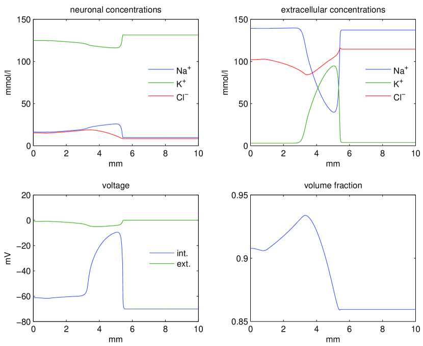
Figure 1: A snapshot of an SD wave at $t=50$s. Plotted are intracellular and extracellular ionic concentrations, intracellular(int.) and extracellular(ext.) voltages and the intracellular volume fraction. Note that the extracellular voltage experiences a negative shift (the negative DC shift).

6.3 Varying gap junctional conductance

We study the dependence of the SD wave speed on the strength of gap junctional conductance. It has been suggested that gap junctional conductance may be necessary for the propagation of SD waves [53], and this was tested using a computational model in [51]. Here, we reexamine this hypothesis.

We vary the value of $\chi$ in (6.5) from $0$ to $10^{-3}$ in increments of $5\times 10^{-5}$. Note that, in [51], $\chi$ was given a value of $1/4$. The resulting SD wave speed is given in Figure 2. We see that even a small increase in gap junctional conductance (far smaller than that postulated in [51]), leads to propagation speeds that exceed physiologically realistic bounds by large margins (typical speeds are $2$ to $7$cm/min). The likely reason for the discrepancy between our computations and those of [51] is that electrotonic coupling is not properly accounted for in [51]. Gap junctional coupling will inevitably lead to cable (or electrotonic) effects, which will enable fast wave propagation as seen in cardiac or skeletal muscle tissue. Constitutively open gap junctions, therefore, are likely not involved in the propagation of SD waves. For the gap junctional hypothesis to be viable, closed gap junctions may have to open with the spread of the wave [53].

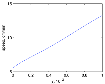
Figure 2: Speed of spreading depression wave as a function of the parameter $\chi$ in (6.5).

6.4 Varying extracellular chloride concentration

The value of the extracellular chloride concentration can be variable, and its effect on SD is not well-understood. Here, we vary the preparatory initial value of extracellular chloride concentration $c_{{\rm Cl}*}^{\rm e}$ between $6$mmol/l and $120$mmol/l and perform computations at $31$ logarithmically equi-spaced values.

A sample plot of the propagating front when $c_{{\rm Cl}*}^{\rm e}=6$mmol/l is given in Figure 3. There are several interesting differences between this and the case $c_{{\rm Cl}*}^{\rm e}=120$mmol/l (shown in Figure 1). First, the spreading depression wave form is altered. The wave in the $c_{{\rm Cl}*}^{\rm e}=6$mmol/l case has longer wavelength, and thus, a longer duration at each spatial location. Another difference is that in the $c_{{\rm Cl}*}^{\rm e}=6$mmol/l case, the change in neuronal volume is small. Given (near) electroneutrality, osmotic pressure change is possible only when both anions and cations can pass the membrane. With little chloride, inward Na⁺ flux cannot be accompanied by a matching inward Cl^- flux. This is in line with the verbal arguments in [53].

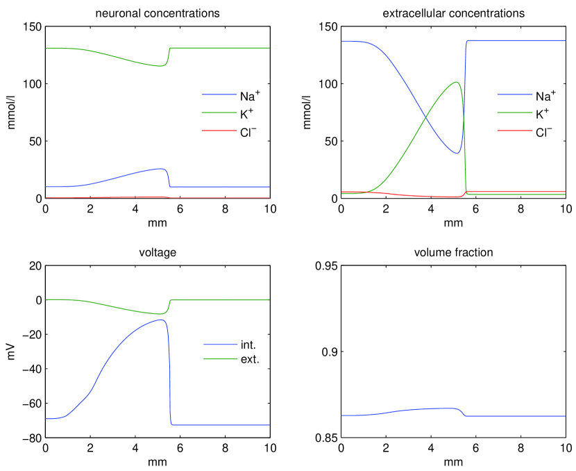
Figure 3: A snapshot of an SD wave at $t=50$s when $c_{{\rm Cl}*}^{\rm e}=6$mmol/l. Compared to Figure 1, the wave is wider and the volume change is minimal.

In Figure 4, we plot the SD propagation speed as a function of $c_{{\rm Cl},0}^{\rm e}$. It is interesting that the dependence is non-monotonic. The reason why the speed increases at low $c_{{\rm Cl},0}^{\rm e}$ is likely because a high chloride concentration has a stabilizing effect on membrane excitability. The reason for the increase in speed at higher chloride concentration may be due to the fact that higher extracellular chloride concentration facilitates potassium diffusion. In order for potassium to diffuse, by (near) electroneutrality, chloride must also diffuse, or a deficit in sodium concentration must be created. The speed of these processes should influence the ease with which potassium can diffuse, and thus, the speed of the SD wave.

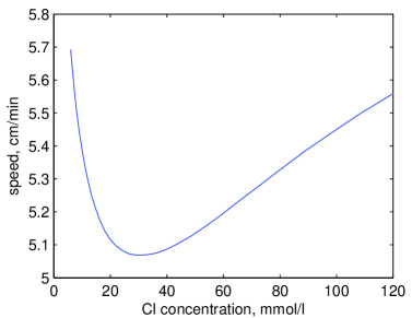
Figure 4: Speed of spreading depression wave as a function of $c_{{\rm Cl}*}^{\rm e}$.

7 Conclusion

In this paper, we formulated a multidomain tissue model of ionic electrodiffusion, volume changes and osmotic water flow. We devised a numerical scheme for one spatial dimension without interstitial flow. This was applied to the study of SD.

An interesting theoretical issue is the relation of this tissue level model to more microscopic cellular level models such as [39]. The cardiac bidomain model can be derived as a formal homogenization limit of a microscopic model [43, 29], and a similar derivation may be possible here.

There is much to be done in terms of numerical algorithms. In the brain, it is increasingly recognized that water flow may play an important physiological role [42], and it is thus of great interest to develop a numerical scheme that can treat water flow. The algorithm presented in Section 5 easily generalizes to two and three spatial dimensions, but the required computational cost may be substantial and much work may be needed for the development of efficient solvers. Another important direction would be to devise numerical methods that exploit the presence of disparate time scales, by updating certain variables at finer time steps than others.

An important feature of the model was that it satisfies an energy identity, and this property may be of direct interest in the study of SD. Indeed, SD is understood as a major breakdown in ionic homeostasis, or dissipation of actively stored free energy [12]. Our model provides a means of quantitatively computing this breakdown.

The SD model used here is limited in several respects, the most important of which is the absence of a glial compartment, which is known to play a significant role in ionic concentration homeostasis and hence in SD [53].

Finally, it should be stressed that the multidomain electrodiffusion model formulated here is not restricted in its application to SD or to brain ionic homeostasis. We hope it would find application in many physiological systems both neural and beyond.

Acknowledgments I would like to thank Bob Eisenberg and Chun Liu for valuable discussion. Bob Eisenberg directed the author’s attention to interstitial flow. Huaxiong Huang and Wei Yao kindly provided their code used in their publication [60]. I also thank the Fields Institute (Toronto, Canada) for the generous support during the Spreading Depression workshop in the summer of 2014. Many participants of the workshop gave me valuable input and much encouragement. This paper is dedicated to Robert Miura, who introduced me to this topic almost ten years ago.

Appendix A Details of Spreading Depression Simulation

A.1 Transmembrane Fluxes

We follow [26, 27, 60] for the transmembrane fluxes. We have:

$$\begin{split}g_{\rm Na}&=j_{\rm NaL}+j_{\rm NaP}+j_{\rm NaE}+2h_{\rm NaK},\\ g_{\rm K}&=j_{\rm KL}+j_{\rm KDR}+j_{\rm KA}+j_{\rm KE}-3h_{\rm NaK},\\ g_{\rm Cl}&=j_{\rm ClL}+j_{\rm ClE}.\end{split}$$ (A.1)

The leak flux $j_{i{\rm L}}$ have the following form (see (3.19)):

$$j_{i{\rm L}}=G_{i}(\mu_{i}^{\rm i}-\mu_{i}^{\rm e})$$ (A.2)

where the conductances $G_{i}(z_{i}F)^{2}$ are given in Table 2.

ion	conductance (mS$/$cm2)	NaK ATPase parameters
Na+	$2\times 10^{-2}$	$I_{\rm max}$	$13$ ($\mu$A/cm2)
K+	$7\times 10^{-2}$	$K_{\rm K}$	$2$ (mmol/l)
Cl-	$2\times 10^{-1}$	$K_{\rm Na}$	$7.7$ (mmol/l)

Table 2: Leak conductances and NaKATPase parameters

The persistent Na⁺ flux $j_{\rm NaP}$ has the following form (see (3.20))

$$j_{\rm NaP}=m_{\rm NaP}^{2}h_{\rm NaP}P_{\rm NaP}J_{\rm GHK}(1,c_{\rm Na}^{\rm i},c_{\rm Na}^{\rm e},\phi_{\rm m})$$ (A.3)

where $P_{\rm NaP}$ is the permeability and $s=m_{{\rm NaP}},h_{{\rm NaP}}$ are the gating variables. The gating variables satisfy the equations:

$$\frac{\partial s}{\partial t}=\alpha_{s}(\phi_{m})(1-s)-\beta_{s}(\phi_{m})s.$$ (A.4)

The form of $j_{\rm KA}$ and $j_{\rm KDR}$ are similar. The parameters and functions defining the above equations are given in Table 3.

flux	$P$ (cm/s)	gates	rate functions (ms-1)
$j_{\rm NaP}$	$2\times 10^{-5}$	$m^{2}h$	$\alpha_{m}$	$=$	$(6(1+\exp(-(0.143\phi_{m}+5.67))))^{-1}$
			$\beta_{m}$	$=$	$1-\alpha_{m}$
			$\alpha_{h}$	$=$	$5.12\times 10^{-6}\exp(-(0.056\phi_{m}+2.94))$
			$\beta_{h}$	$=$	$1.6\times 10^{-4}(1+\exp(-(0.2\phi_{m}+8)))^{-1}$
$j_{\rm KDR}$	$1\times 10^{-3}$	$m^{2}$	$\alpha_{m}$	$=$	$0.08\varphi(0.2\phi_{\rm m}+6.98)$
			$\beta_{m}$	$=$	$0.25\exp(-(0.25\phi_{\rm m}+1.25))$
$j_{\rm KA}$	$1\times 10^{-4}$	$m^{2}h$	$\alpha_{m}$	$=$	$0.2\varphi(0.1\phi_{\rm m}+5.69)$
			$\beta_{m}$	$=$	$0.175\widehat{\varphi}(0.1\phi_{\rm m}+2.99)$
			$\alpha_{h}$	$=$	$0.016\exp(-(0.056\phi_{\rm m}+4.61))$
			$\beta_{h}$	$=$	$0.5(1+\exp(-(0.2\phi_{\rm m}+11.98)))^{-1}$

Table 3: Ion fluxes and their corresponding parameters and rate functions. In the above, $P$ is the permeability, $\varphi(u)=u/(1-\exp(-u)),\widehat{\varphi}(u)=u/(\exp(u)-1)$ and the membrane potential $\phi_{\rm m}$ is in mV.

The excitation currents $j_{i{\rm E}}$ are used to initiate the spreading depression wave. This is described in (6.8) of Section 6.2.

The Na⁺ and K⁺ flux carried by the NaK ATPase is given by $3h_{\rm NaK}$ and $-2h_{\rm NaK}$ respectively in (A.1). Here, $h_{\rm NaK}$ is given by

$$h_{\rm NaK}=\widehat{I}_{\rm max}(1+K_{\rm K}/c_{\rm K}^{\rm e})^{-2}(1+K_{\rm Na}/c_{\rm Na}^{\rm i})^{-3}$$ (A.5)

where the constants $I_{\rm max}=\widehat{I}_{\rm max}F,K_{\rm K}$ and $K_{\rm Na}$ are given in Table 2.

A.2 Initial Conditions

We first set preparatory initial data and run the model to steady state. These steady state values are then used as initial data to run the model simulations (with $0$ excitatory fluxes).

The list of preparatory initial data for the concentrations $c_{i}^{k}$ and membrane potential $\phi_{\rm m}$, and volume fraction $\alpha_{k}$ are given in Table 4. The preparatory initial value for intracellular chloride is given by the expression

$$c_{{\rm Cl}*}^{\rm i}=c_{{\rm Cl}*}^{\rm e}\exp(\phi_{{\rm m}*}F/RT)$$ (A.6)

where the subscript $*$ refers to the preparatory initial values. Once these preparatory initial value are given, we may compute the impermeable solute amount $a_{k}$ by solving (2.11) for $a_{k}$:

$$a_{k}=-\frac{1}{z_{0}^{k}}\sum_{i=1}^{M}z_{i}\alpha_{k}^{*}c_{i*}^{k}.$$ (A.7)

$\alpha_{\rm i}$	$1/1.15$	$\phi_{\rm m}$	$-70$(mV)
$c_{\rm Na}^{\rm i}$	$10$	$c_{\rm Na}^{\rm e}$	$145$
$c_{\rm K}^{\rm i}$	$130$	$c_{\rm K}^{\rm e}$	$3.5$
$c_{\rm Cl}^{\rm i}$	$-$	$c_{\rm Cl}^{\rm e}$	$120$

Table 4: Preparatory initial values. Concentrations are in mmol/l. For intracellular chloride concentration, see (A.6). Note that $\alpha_{\rm e}$ is set to $1-\alpha_{\rm i}$ (see (2.1)).

The preparatory initial values of the gating variables are set to the steady state values of (A.4):

$$s=\frac{\alpha_{s}(\phi_{{\rm m}*})}{\alpha_{s}(\phi_{{\rm m}*})+\beta_{s}(\phi_{{\rm m}*})}.$$ (A.8)

Given these preparatory initial conditions, the model is run to steady state with no excitatory fluxes ($j_{i{\rm E}}=0$ in (A.1)) and $\Delta t=10$s. The preparatory run is terminated when the discrete time derivative of the ionic concentrations falls below $10^{-12}$ times the maximum ionic concentration. We note that the difference between the preparatory initial values and the steady state values are typically very small.

Appendix B Computation of Extracellular Voltage

In our model, the extracellular voltage is computed as a natural output of the system of equations, and we cannot, in general, compute the membrane potential without computing both the extracellular and intracellular voltages (and the other compartmental voltages if there are more than two compartments). There is, however, a special situation in which the membrane potential can be computed without computing the extracellular voltage. We discuss this special case, as it relates to previous attempts in obtaining the extracellular voltage [1, 2]. Let us restrict our attention to the two compartment case without fluid flow in one spatial dimension. We let the equations be satisfied on the interval $0<x<L$. We adopt the notation of Section 6.1. Let us assume furthermore that gap junctional coupling is absent ($D_{i}^{\rm i}=0$). Taking the time derivative of the first equality in (6.6) and using (6.3), we have:

$$\gamma C_{\rm m}\frac{\partial\phi_{\rm m}}{\partial t}=\sum_{i=1}^{M}\gamma g_{i},$$ (B.1)

where we used our assumption $D_{i}^{\rm i}=0$. The above equation does not explicitly depend on $\phi_{\rm i}$ or $\phi_{\rm e}$, and only on the membrane potential $\phi_{\rm m}$, since the transmembrane fluxes $g_{i}$ depend on voltage only through $\phi_{\rm m}$. Now, let us use the electroneutrality relation in place of the charge capacitor relation (6.6):

$$0=z_{0}^{\rm i}Fa_{\rm i}+\sum_{i=1}^{3}z_{i}F\alpha_{\rm i}c_{i}^{\rm i}=-\left(z_{0}^{\rm e}Fa_{\rm e}+\sum_{i=1}^{3}z_{i}F\alpha_{\rm e}c_{i}^{\rm e}\right),\;\phi_{\rm m}=\phi_{\rm i}-\phi_{\rm e}.$$ (B.2)

Then (B.1) reduces further to:

$$\sum_{i=1}^{M}\gamma g_{i}=0.$$ (B.3)

Equations (B.1) and (B.3) are often used in modeling studies to obtain the membrane potential. Note, however, that this is valid only when there is no gap junctional coupling.

Let us now take the derivative of the second equality in (B.2) with respect to $t$. Using (6.2) and (B.3), we have

$$\frac{\partial}{\partial x}\left(a+\sigma\frac{\partial\phi_{\rm e}}{\partial x}\right)=0,\;a=\sum_{i=1}^{M}z_{i}FD_{i}^{\rm e}\frac{\partial c_{i}^{\rm e}}{\partial x},\;\sigma=\sum_{i=1}^{M}\frac{(z_{i}F)^{2}D_{i}^{\rm e}c_{i}^{\rm e}}{RT}.$$ (B.4)

This is the same as (4.19) except that the capacitor term and the advective current terms are absent. Assuming no-flux boundary conditions at $x=0$ and $x=L$, we obtain, from the above:

$$a+\sigma\frac{\partial\phi_{\rm e}}{\partial x}=0.$$ (B.5)

This is the relation used to determine the extracellular voltage in [1, 2]. It should be emphasized, however, that one may use the above expression to compute the extracellular voltage only under the restrictive conditions of no gap junctional coupling, one-dimensional geometry and no-flux boundary conditions. Otherwise, the charge capacitor relation (or equivalently, near electroneutrality) will be violated.

References

• [1] Antônio-Carlos G Almeida, HZ Texeira, Mário A Duarte, and Antonio Fernando C Infantosi. Modeling extracellular space electrodiffusion during lea  o’s spreading depression. Biomedical Engineering, IEEE Transactions on, 51(3):450–458, 2004.
• [2] Max R Bennett, Les Farnell, and William G Gibson. A quantitative model of cortical spreading depression due to purinergic and gap-junction transmission in astrocyte networks. Biophysical journal, 95(12):5648–5660, 2008.
• [3] W.F. Boron and E.L. Boulpaep. Medical physiology. W.B. Saunders, 2nd edition, 2008.
• [4] JC Chang, KC Brennan, D He, H Huang, RM Miura, PL Wilson, and JJ Wylie. A mathematical model of the metabolic and perfusion effects on cortical spreading depression. PLoS One, 8(8):e70469, August 2013.
• [5] A. Charles and KC Brennan. Cortical spreading depression new insights and persistent questions. Cephalalgia, 29(10):1115–1124, 2009.
• [6] Haoran Chen, Maria-Carme Calderer, and Yoichiro Mori. Analysis and simulation of a model of polyelectrolyte gel in one spatial dimension. Nonlinearity, 27(6):1241, 2014.
• [7] M.A. Dahlem, R. Graf, A.J. Strong, J.P. Dreier, Y.A. Dahlem, M. Sieber, W. Hanke, K. Podoll, and E. Schöll. Two-dimensional wave patterns of spreading depolarization: Retracting, re-entrant, and stationary waves. Physica D: Nonlinear Phenomena, 239(11):889–903, 2010.
• [8] Markus A Dahlem. Migraines and cortical spreading depression. In Encyclopedia of Computational Neuroscience, pages 1–9. Springer, 2014.
• [9] M. Doi and S.F. Edwards. The theory of polymer dynamics. International series of monographs on physics. Clarendon Press, 1988.
• [10] Masao Doi. Onsager’s variational principle in soft matter. Journal of Physics: Condensed Matter, 23(28):284118, 2011.
• [11] CORINA S Drapaca and JASON S Fritz. A mechano-electrochemical model of brain neuro-mechanics: application to normal pressure hydrocephalus. Int. J. Num. Anal. Mod. Ser. B, 1:82–93, 2012.
• [12] Jens P Dreier, Thomas Isele, Clemens Reiffurth, Nikolas Offenhauser, Sergei A Kirov, Markus A Dahlem, and Oscar Herreras. Is spreading depolarization characterized by an abrupt, massive release of gibbs free energy from the human brain cortex? The Neuroscientist, 19(1):25–42, 2013.
• [13] J.P. Dreier. The role of spreading depression, spreading depolarization and spreading ischemia in neurological disease. Nature medicine, 17(4):439–447, 2011.
• [14] D.A. Drew and S.L. Passman. Theory of Multicomponent Fluids. Applied Mathematical Sciences. Springer New York, 2012.
• [15] B. Eisenberg, Y.K. Hyon, and C. Liu. Energy variational analysis of ions in water and channels: Field theory for primitive models of complex ionic fluids. The Journal of Chemical Physics, 133:104104, 2010.
• [16] R. S Eisenberg and E. A Johnson. Three-dimensional electrical field problems in physiology. Prog. Biophys. Mol. Biol, 20(1), 1970.
• [17] RS Eisenberg, V. Barcilon, and RT Mathias. Electrical properties of spherical syncytia. Biophysical Journal, 25(1):151–180, 1979.
• [18] B. Grafstein. Mechanism of spreading cortical depression. Journal of Neurophysiology, 19(2):154–171, 1956.
• [19] Berenice Grafstein. Neuronal release of potassium during spreading depression. Brain function, 1:87–124, 1963.
• [20] WY Gu, WM Lai, and VC Mow. A mixture theory for charged-hydrated soft tissues containing multi-electrolytes: passive transport and swelling behaviors. Journal of biomechanical engineering, 120:169–180, 1998.
• [21] WM Gu WY, Lai and VC Mow. Transport of multi-electrolytes in charged hydrated biological soft tissues. Transport in Porous Media, 34(1):143–157, 1999.
• [22] Craig S Henriquez. Simulating the electrical behavior of cardiac tissue using the bidomain model. Critical reviews in biomedical engineering, 21(1):1–77, 1992.
• [23] O. Herreras, G. Somjen, and A. Strong. Electrical prodromals of spreading depression void grafstein s potassium hypothesis. Journal of neurophysiology, 94(5):3656–3657, 2005.
• [24] F.C. Hoppensteadt and C.S. Peskin. Modeling and simulation in medicine and the life sciences. Springer Verlag, 2002.
• [25] Y. Hyon, DY Kwak, and C. Liu. Energetic variational approach in complex fluids: Maximum dissipation principle. DCDS-A, 26(4):1291–1304, 2010.
• [26] H. Kager, WJ Wadman, and GG Somjen. Simulated seizures and spreading depression in a neuron model incorporating interstitial space and ion concentrations. Journal of neurophysiology, 84(1):495, 2000.
• [27] H. Kager, WJ Wadman, and GG Somjen. Conditions for the triggering of spreading depression studied with computer simulations. Journal of neurophysiology, 88(5):2700–2712, 2002.
• [28] A. Katzir-Katchalsky and P.F. Curran. Nonequilibrium thermodynamics in biophysics. Harvard University Press, 1965.
• [29] J.P. Keener and J. Sneyd. Mathematical Physiology. Springer-Verlag, New York, 1998.
• [30] C. Koch. Biophysics of Computation. Oxford University Press, New York, 1999.
• [31] Aristides AP Leao. Spreading depression of activity in the cerebral cortex. Journal of Neurophysiology, 1944.
• [32] BK Leung, JA Bonanno, and CJ Radke. Oxygen-deficient metabolism and corneal edema. Progress in retinal and eye research, 30(6):471–492, 2011.
• [33] F.H. Lynch. Mathematical Modeling of the Gastric Mucus Gel. PhD thesis, University of Utah, 2011.
• [34] Duane Malcolm. A Computational Model of the Ocular Lens. PhD thesis, University of Auckland, 2007.
• [35] Hiss Martins-Ferreira, Maiken Nedergaard, and Charles Nicholson. Perspectives on spreading depression. Brain research reviews, 32(1):215–234, 2000.
• [36] RM Miura, H. Huang, and JJ Wylie. Cortical spreading depression: An enigma. The European Physical Journal-Special Topics, 147(1):287–302, 2007.
• [37] Y. Mori. Mathematical Properties of Pump-Leak Models of Cell Volume Control and Electrolyte Balance. Journal of Mathematical Biology, 64:873–916, 2012.
• [38] Y. Mori, G. I. Fishman, and C. S Peskin. Ephaptic conduction in a cardiac strand model with 3D electrodiffusion. Proceedings of the National Academy of Sciences, 105(17):6463, 2008.
• [39] Y. Mori, C. Liu, and R.S. Eisenberg. A Model of Electrodiffusion and Osmotic Water Flow and its Energetic Structure. Physica D: Nonlinear Phenomena, 240:1835–1852, November 2011.
• [40] Y. Mori and C.S. Peskin. A numerical method for cellular electrophysiology based on the electrodiffusion equations with internal boundary conditions at internal membranes. Communications in Applied Mathematics and Computational Science, 4:85–134, 2009.
• [41] Yoichiro Mori, Haoran Chen, Catherine Micek, and Maria-Carme Calderer. A dynamic model of polyelectrolyte gels. SIAM Journal on Applied Mathematics, 73(1):104–133, 2013.
• [42] Maiken Nedergaard. Garbage truck of the brain. Science, 340(6140):1529–1530, 2013.
• [43] J.C. Neu and W. Krassowska. Homogenization of syncytial tissues. Critical reviews in biomedical engineering, 21(2):137–199, 1993.
• [44] C Nicholson. Volume transmission and the propagation of spreading depression. Migraine: Basic Mechanisms and Treatment, pages 293–308, 1993.
• [45] W. Nonner, D.P. Chen, and B. Eisenberg. Progress and prospects in permeation. J. Gen. Physiol., 113(6):773–782, 1999.
• [46] L. Onsager. Reciprocal Relations in Irreversible Processes. II. Physical Review, 38(12):2265–2279, 1931.
• [47] N. Qian and T.J. Sejnowski. An electro-diffusion model for computing membrane potentials and ionic concentrations in branching dendrites, spines and axons. Biol. Cybern., 62:1–15, 1989.
• [48] J.A. Reggia and D. Montgomery. A computational model of visual hallucinations in migraine. Computers in biology and medicine, 26(2):133–141, 1996.
• [49] LV Reshodko and J Bureš. Computer simulation of reverberating spreading depression in a network of cell automata. Biological cybernetics, 18(3-4):181–189, 1975.
• [50] K. Revett, E. Ruppin, S. Goodall, and J.A. Reggia. Spreading depression in focal ischemia: A computational study. Journal of Cerebral Blood Flow & Metabolism, 18(9):998–1007, 1998.
• [51] B.E. Shapiro. Osmotic forces and gap junctions in spreading depression: a computational model. Journal of Computational Neuroscience, 10(1):99–120, 2001.
• [52] G.G. Somjen. Mechanisms of spreading depression and hypoxic spreading depression-like depolarization. Physiological reviews, 81(3):1065, 2001.
• [53] G.G. Somjen. Ions in the Brain. Oxford University Press, 2004.
• [54] HC Tuckwell and RM Miura. A mathematical model for spreading cortical depression. Biophysical Journal, 23(2):257–276, 1978.
• [55] Henry C Tuckwell. Simplified reaction-diffusion equations for potassium and calcium ion concentrations during spreading cortical depression. International Journal of Neuroscience, 12(2):95–107, 1981.
• [56] Leslie Tung. A bi-domain model for describing ischemic myocardial dc potentials. PhD thesis, Massachusetts Institute of Technology, 1978.
• [57] Guo-Wei Wei, Qiong Zheng, Zhan Chen, and Kelin Xia. Variational multiscale models for charge transport. SIAM Review, 54(4):699–754, 2012.
• [58] AM Weinstein. Ammonia transport in a mathematical model of rat proximal tubule. American Journal of Physiology-Renal Physiology, 267(2):F237–F248, 1994.
• [59] AM Weinstein. Mathematical models of tubular transport. Annual review of physiology, 56(1):691–709, 1994.
• [60] Wei Yao, Huaxiong Huang, and Robert M Miura. A continuum neuronal model for the instigation and propagation of cortical spreading depression. Bulletin of mathematical biology, 73(11):2773–2790, 2011.