Molecular theory of
anomalous diffusion

Abstract

The nonlinear theory of anomalous diffusion is based on particle interactions giving an explicit microscopic description of diffusive processes leading to sub-, normal, or super-diffusion as a result competitive effects between attractive and repulsive interactions. We present the explicit analytical solution to the nonlinear diffusion equation which we then use to compute the correlation function which is experimentally measured by correlation spectroscopy. The theoretical results are applicable in particular to the analysis of fluorescence correlation spectroscopy of marked molecules in biological systems. More specifically we consider the case of fluorescently labeled lipids and we find that the nonlinear correlation spectrum reproduces very well the experimental data indicating sub-diffusive molecular motion of lipid molecules in the cell membrane.

1 Classical diffusion and anomalous diffusion

There are many systems observed in nature and in the laboratory where it seems natural to use the language of diffusion, but where one finds that the space or time dispersion of the diffusing objects do not obey the classical diffusion equation, which is an indication that the objects do not move ”freely”: obstacles, time delays, interactions can modify their trajectories in such a way that their mean squared displacement deviates from the classical linear law $\langle r^{2}\rangle\sim t$ and the Gaussian structure of the dispersion is deformed or replaced by a different distribution. Such non-classical distributions with non-exponential behavior are generally the signature of anomalous diffusion and the mean squared displacement then follows a power law in the time variable: $\langle r^{2}\rangle\sim t^{{\gamma}}$ with $0<{\gamma}\neq 1$ (while ${\gamma}=1$ for regular diffusion). Depending on whether ${\gamma}<1$ or ${\gamma}>1$, one talks about sub-diffusion when the particles are e.g. delayed in their diffusive motion by the presence of obstacles or because of the structural complexity of the medium or because of molecular interactions, and super-diffusion when their motion is e.g. enhanced by concentration effects or by an external field.

Fundamental constraints in constructing a theory of anomalous diffusion are then needed to reproduce a mean-squared displacement that exhibits power-law behavior as a function of time and the fundamental demand for the existence of self-similar solutions, i.e. such that all moments scale similarly, $\langle r^{2n}\rangle\sim t^{n\gamma}$. This implies that the distribution should have the form $f(r,t)=t^{-\gamma/2}\phi(r/t^{\gamma/2})$ for some function $\phi(x)$ (as is the case for classical diffusion).

In Einstein’s random walk model einstein , the jumps can extended to lengths greater than one with different probabilities including rests (jumps of length zero) without affecting the diffusive nature of the process. Generally, diverse microscopic dynamics can give rise to ”diffusion” phenomena at the macroscopic level, but the underlying mechanisms may be quite different; for instance the distinction should be made between molecular diffusion of tagged particles which, while identical to the medium particles, are made observable by radioactive or fluorescent markers RNA_Diff ; molecularD and tracer diffusion where experimentally one follows trajectories of distinguishable particles seeded in an active medium  sanchez ; dogariu .

Various approaches for a general description of diffusive phenomena have been developed in the past few years. They can be divided into three classes:

(i) the fractional Fokker-Planck equation (FFPE) is based on the continuous time random walk model with a power law ansatz for the distribution of the time delays in the motion of the particles FFPE_PhysToday and describes the phenomenology of sub-diffusion Metzler_Review ; Barkai_Review ;

(ii) the fractional Brownian motion uses a generalized random walk model with correlations between particle displacements leading to a diffusion equation with classical structure, but with time-dependent coefficients fBm1 ; fBm2 ;

(iii) the nonlinear Fokker-Planck equation (NLFP) for anomalous diffusion, which we use in the present analysis, is obtained from a generalization of Einstein’s mean field equation for the random walk by allowing the probability for a jump from one site to another to depend on the walkers concentration. When this microscopic dynamics is constrained by the demand for diffusive-like scaling solutions, it is found BoonLutsko ; LutskoBoon8 that the jump probabilities must have the form of a power law $\sim f^{(\alpha-1)}(r,t)$, where $f(r,t)$ is the probability that a random walker be at position $r$ at time $t$. This approach provides a molecular theory of anomalous diffusion based on particle interactions leading to sub- or super-diffusion (see Fig.1 in LutskoBoon13 ) as a result of a balance between attractive and repulsive interactions.

In the next section, we review the nonlinear theory of anomalous diffusion and its main result, the nonlinear Fokker-Plank equation (NLFP) whose solutions are given explicitly in Section 3 and further discussed in Sections 4 and 5. Fluorescence correlation spectroscopy (FCS) is an interesting light scattering method which can be used to measure molecular diffusion in biological systems and thereby detect anomalous diffusion. The FCS correlation spectrum is computed analytically (i) for the case of classical diffusion in Section 6 and (ii) for anomalous diffusion using the distribution function obtained from the NLFP solution in Section 7 where the analytical results are compared with experimental data for the case of lipid molecules diffusion in cell membranes.

2 The generalized Fokker-Plank equation

Generalizing the jump probabilities $P_{j}$ in Einstein’s master equation by introducing a functional dependence on the distribution functions $f(r,t)$ at the starting point $r-j$ and at the end point $r$ of the jump, we have

$$P_{j}={p}_{j}\,{F}[f(r-j\,\delta r,t),f(r,t)]\,,\;\;\;\;\;\mbox{with}\;\;\;\;\sum_{j}\,\,P_{j}=1\,,$$ (1)

where the probabilities ${p}_{j}$ are drawn from a prescribed distribution and the bounding condition $0\leq P_{j}\leq 1$ imposes $0\leq F(x,y)\leq 1$ as well as restrictions on the functional form of $F(x,y)\doteqdot{F}[f(r-j\,\delta r,t),f(r,t)]$. Under these conditions, multiscale expansion of the master equation is shown to give the generalized Fokker-Planck (or generalized diffusion) equation LutskoBoon13

$$\frac{\partial f}{\partial t}+M_{1}\frac{\partial}{\partial r}\left[xF\left(x,x\right)\right]_{f}$$ (2)

$$=M_{2}\frac{\partial}{\partial r}\left[\frac{\partial xF\left(x,y\right)}{\partial x}-\frac{\partial xF\left(x,y\right)}{\partial y}\right]_{f}\frac{\partial f}{\partial r}$$

$$+\frac{1}{2}M_{1}^{2}\delta t\frac{\partial}{\partial r}\left[\frac{\partial xF\left(x,y\right)}{\partial x}-\frac{\partial xF\left(x,y\right)}{\partial y}-\left(\frac{\partial xF\left(x,x\right)}{\partial x}\right)^{2}\right]_{f}\frac{\partial f}{\partial r}\,,$$

with the notation

$$\left[\frac{\partial xF\left(x,y\right)}{\partial x}\right]_{f}=\left[\frac{\partial xF\left(x,y\right)}{\partial x}\right]_{x=f\left(r,t\right),y=f\left(r,t\right)}\,.$$ (3)

In Eq.(2), $M_{1}$ and $M_{2}$ are given by

$$M_{1}=\frac{\delta r}{\delta t}\,\sum_{j}\,j\,p_{j}=\frac{\delta r}{\delta t}\,J_{1}\,,$$

$$M_{2}=\frac{1}{2}\frac{\left(\delta r\right)^{2}}{\delta t}\left(\left(\sum_{j}\,j^{2}\,p_{j}\right)-J_{1}^{2}\right)=\frac{1}{2}\frac{\left(\delta r\right)^{2}}{\delta t}\left(J_{2}-J_{1}^{2}\right)$$ (4)

where the $J_{n}$’s denote the moments $J_{n}=\sum_{j}j^{n}p_{j}$. Note that for $F\left(x,y\right)=1$, Eq.(2) reduces to the classical advection-diffusion equation.

Since the function $F\left(x,y\right)$ is defined in terms of the jump probabilities, it must be bounded, and so must satisfy

$$0\leq xF\left(x,y\right)\leq 1\;\;\;\;\mbox{and}\;\;\;\;0\leq yF\left(x,y\right)\leq 1\,,\;\;\;\;\forall\;x,y\in\left[0,1\right]\,.$$ (5)

It was shown in LutskoBoon13 that self-similar solutions are possible if and only if

$$\lim_{y\rightarrow x}\left[\frac{\partial xF\left(x,y\right)}{\partial x}-\frac{\partial xF\left(x,y\right)}{\partial y}\right]\sim x^{\alpha-1}$$ (6)

where the scaling exponent $\alpha$ is related to the diffusion exponent by

$$\gamma=\frac{2}{\alpha+1}\;.$$ (7)

Anomalous (sub- and super-) diffusion can be described in a single formulation when the jump probabilities have the following form in terms of the occupation probabilities

$${F}(x,y;\omega_{s},\omega_{e})\sim\omega_{s}\,F_{s}(x)+\omega_{e}\,F_{e}(y)\,;$$ (8)

here $\omega_{s}$ and $\omega_{e}$ are weighting factors relative to the functionals of the concentrations at the starting point and at the end point of the jump. Using the notation $a\equiv\omega_{e}/\omega_{s}$ , (8) is rewritten in normalised form as

$$F(x,y;a)=\frac{F(x)+aF(y)}{F(x)+F(y)}.$$ (9)

where the positivity arguments, $x,y$ and the constraints (5) and $F(x,y;a)\geq~{}0$ imply that $0\leq a\leq 1$.

Considering the case that there is no drift ($M_{1}=0$ in Eq.(2)), and in order that the general formulation describe diffusion, we should have a scaling solution of the form $f\left(r,t\right)=t^{-\gamma/2}\phi\left(r/t^{\gamma/2}\right)$ which demands that LutskoBoon13

$$\lim_{y\rightarrow x}\left(\frac{\partial}{\partial x}xF\left(x,y;a\right)-\frac{\partial}{\partial y}xF\left(x,y;a,\alpha\right)\right)=K\,x^{\alpha-1}\,,$$ (10)

for some constant $\alpha$. Using (9) in the l.h.s of (10) gives

$$\frac{1+a}{2}+\frac{1-a}{2}\frac{x\,F^{\prime}\left(x\;a,\alpha\right)}{\,F\left(x;a,\alpha\right)} =K\,x^{\alpha-1}\,,$$ (11)

which is solved to yield

$$F\left(x;a,\alpha\right) =\frac{B}{x^{\frac{1+a}{1-a}}}\,\exp{\left(\frac{2\,K}{1-a}\,\frac{x^{\alpha-1}}{\alpha-1}\right)}\,,$$ (12)

where $B$ is an integration constant; reinserting (12) into (9), we find

$$F(x,y;a,\alpha)=\frac{1+a\,\left(\frac{x}{y}\right)^{\frac{1+a}{1-a}}\,\exp\left(\frac{2\,K}{1-a}\,\frac{y^{{\alpha-1}}-x^{{\alpha-1}}}{\alpha-1}\right)}{1+\left(\frac{x}{y}\right)^{\frac{1+a}{1-a}}\,\exp\left(\frac{2\,\lambda}{1-a}\,\frac{y^{{\alpha-1}}-x^{{\alpha-1}}}{\alpha-1}\right)}\,.$$ (13)

The natural limit: $\lim_{{{\alpha\rightarrow 1}}}F(x,y;a)=1$ requires $K=\frac{1}{2}(1+a)\,\lambda^{\alpha-1}$ where $\lambda$ is an unitary constant with the dimension of length. Thus,

$$F(x,y;a,\alpha)=\frac{1+a\,G(x,y;a,\alpha)}{1+G(x,y;a,\alpha)}\,,$$ (14)

with

$${G(x,y;a,\alpha)}\,=\,\left(\frac{x}{y}\right)^{\frac{1+a}{1-a}}\,\exp\left(\frac{1+a}{1-a}\;\lambda^{\alpha-1}\,\frac{y^{{\alpha-1}}-x^{{\alpha-1}}}{\alpha-1}\right)\;.$$ (15)

It is clear that for any finite value $x>0$, $0\leq F(x,y;a,\alpha)<1\;\;,\forall\;y\in\left[0,1\right]\,$ and that the limit $F(x,y;a=1,\alpha\rightarrow 1)=~{}1$ gives normal diffusion. Furthermore

$$\lim_{x\rightarrow 0}F(x,y;a,\alpha)=\left\{\begin{array}[]{c}1,\;\;\;\alpha>1\\ a,\;\;\;\alpha<1\end{array}\right.\;\;\;\mbox{;}\;\;\lim_{y\rightarrow 0}F(x,y;a,\alpha)=\left\{\begin{array}[]{c}a,\;\;\;\alpha>1\\ 1,\;\;\;\alpha<1\end{array}\right.$$ (16)

Physical interpretation.

To provide some interpretation, we note that

$$\frac{\partial}{\partial x}F(x,y;a,\alpha) =(1+a)\,\frac{G(x,y;a,\alpha)}{\left({1+G(x,y;a,\alpha)}\right)^{2}}\,\left(\frac{(\lambda\,x)^{\alpha-1}-1}{x}\right)\;,$$ (17)

$$\frac{\partial}{\partial y}F(x,y;a,\alpha) =(1+a)\,\frac{G(x,y;a,\alpha)}{\left({1+G(x,y;a,\alpha)}\right)^{2}}\,\left(\frac{1-(\lambda\,y)^{\alpha-1}}{y}\right)\;.$$ (18)

Since $0<x,y<1$, the signs of these derivatives are determined by the factors on the right: $\left((\lambda\,x)^{\alpha-1}-1\right)$ and $\left(1-(\lambda\,y)^{\alpha-1}\right)$, and so depend on whether ($\alpha-1$) is positive or negative:

$$\alpha >1\Longrightarrow\frac{\partial}{\partial x}F(x,y;a,\alpha)<0<\frac{\partial}{\partial y}F(x,y;a)$$

$$\alpha <1\Longrightarrow\frac{\partial}{\partial x}F(x,y;a,\alpha)>0>\frac{\partial}{\partial y}F(x,y;a)$$ (19)

In the first case, $\alpha>1$, the jump probability decreases with the concentration at the starting point and increases with the concentration at the arrival site; in other words the jump rate is reduced by putting more walkers at the origin and increased by putting more at the terminus of a jump: this is analogous to an attractive interaction. For $\alpha<1$, we have the reverse situation: the jump rate is increased by putting more walkers at the origin and decreased by putting more at the terminus, thus emulating a repulsive interaction. In the standard problem with all walkers at the origin at $t=0$, the distribution decays monotonically away from the origin; thus, if the particles repel, the distribution expands faster (i.e. tends to a uniform distribution more quickly) whereas if they attract, then this attraction slows down the spread of the distribution. The physical interpretation is that attractive interactions give sub-diffusion and repulsive interactions give super-diffusion.

3 Solutions of the nonlinear diffusion equation

In the absence of drift, the generalized Fokker-Plank equation, Eq.(2) with (14) and (15), gives the nonlinear diffusion equation Muskat

$$\frac{\partial f(r,t)}{\partial t}=\lambda^{\alpha-1}\frac{1+a}{2\,\alpha}\,M_{2}\frac{\partial^{2}}{\partial r^{2}}\,f^{\alpha}(r,t)\,,$$ (20)

(here $M_{2}=\frac{1}{2}\frac{\left(\delta r\right)^{2}}{\delta t}\,\sum_{j}\,j^{2}\,p_{j}$) and the scaling solutions are obtained following the development given in LutskoBoon13 yielding

$$f\left(r,t\right)=t^{-\gamma/2}\,W\left(1\pm V\,\frac{r^{2}}{t^{\gamma}}\right)^{1/(\alpha-1)}\,,$$ (21)

where $W$ and $V$ are determined by the normalization condition (see below) and by the expression obtained by inserting (21) into (20)

$$VW^{\alpha-1}=\lambda^{1-\alpha}\,\frac{|1-\alpha|}{1+\alpha}\,\frac{1}{1+a}\,{M_{2}}^{-1}\,.$$ (22)

(i) Super-diffusive case.

For $\alpha<1$,

$$f\left(r,t\right)=t^{-\gamma/2}\,W\left(1+V\,\frac{r^{2}}{t^{\gamma}}\right)^{1/(\alpha-1)}\,.$$ (23)

The normalization condition (using the reduced variable $\zeta=V^{1/2}\,\frac{r}{t^{\gamma/2}}$) reads

$$W\,V^{-1/2}\,\int_{-\infty}^{\infty}\,d\zeta\,\left(1+\zeta^{2}\right)^{1/(\alpha-1)}=1\;\;\;\Longrightarrow\;\;\;\frac{W}{\sqrt{V}}=\frac{1}{\sqrt{\pi}}\,\frac{\Gamma(\frac{1}{1-\alpha})}{\Gamma(\frac{1}{1-\alpha}-\frac{1}{2})}\,,$$

provided

$$\frac{\alpha+1}{\alpha-1}<0\;\;\;\Longrightarrow\;\;\;-1<\alpha<1\,\;\;\;\Longrightarrow\;\;\;\gamma>1\,,$$ (24)

and the mean-squared displacement $\left\langle r^{2}\right\rangle=\int_{-\infty}^{\infty}r^{2}f\left(r;t\right)dr$ is given by

$$\left\langle r^{2}\right\rangle = t^{\gamma}\,W\,V^{-3/2}\int_{-\infty}^{\infty}d\zeta\,\zeta^{2}\left(1+\zeta^{2}\right)^{1/(\alpha-1)}$$ (25)

$$= \,\frac{W}{\sqrt{V}}\,\frac{t^{\gamma}}{V}\,\frac{\sqrt{\pi}}{2}\frac{\Gamma(\frac{3\alpha-2}{2(1-\alpha)})}{\Gamma(\frac{1}{1-\alpha})}\,=\,\frac{t^{\gamma}}{V}\,\frac{\Gamma(\frac{3\alpha-2}{2(1-\alpha)})}{2\,\Gamma(\frac{1+\alpha}{2(1-\alpha)})}\,,$$

which is finite if

$$\frac{3\alpha-1}{\alpha-1}<0\;\;\;\Longrightarrow\;\;\;\frac{1}{3}<\alpha<1\;\;\;\Longrightarrow\;\;\;\frac{3}{2}>\gamma>1\,.$$ (26)

(ii) Sub-diffusive case.

For $0<\gamma<1$ i.e. $\alpha>1$ the distribution has finite support so that

$$f\left(r,t\right)=t^{-\gamma/2}\,W\left(1-V\,\frac{r^{2}}{t^{\gamma}}\right)^{1/(\alpha-1)}\Theta\left(1-V\,\frac{r^{2}}{t^{\gamma}}\right)\,,$$ (27)

with the normalization condition

$$W\,V^{-1/2}\,\int_{-1}^{1}\,d\zeta\,\left(1-\zeta^{2}\right)^{1/(\alpha-1)}=1\;\;\;\Longrightarrow\;\;\;\frac{W}{\sqrt{V}}=\frac{1}{\sqrt{\pi}}\,\frac{\Gamma(\frac{2\alpha}{\alpha-1}+1)}{\Gamma(\frac{1}{\alpha-1}+1)}\,,$$

and the mean-squared displacement reads

$$\left\langle r^{2}\right\rangle = t^{\gamma}\,W\,V^{-3/2}\int_{-1}^{1}d\zeta\zeta^{2}\left(1-\zeta^{2}\right)^{1/(\alpha-1)}$$ (28)

$$= \,\frac{W}{\sqrt{V}}\,\frac{t^{\gamma}}{V}\,\frac{\sqrt{\pi}}{2}\,\frac{\Gamma(\frac{1}{\alpha-1}+1)}{\Gamma(\frac{1}{\alpha-1}+\frac{5}{2})}\,=\,\frac{t^{\gamma}}{V}\,\,\frac{\Gamma(\frac{3\alpha-1}{\alpha-1})}{2\,\Gamma(\frac{5\,\alpha-3}{\alpha-1})}\,.$$

4 The anomalous diffusion coefficient

The continuum results imply that an initial distribution of the form $f_{0}(r)=W^{\prime}\,(1+s_{\alpha}\left(r/w\right)^{2})^{1/(\alpha-1)}_{+}$ with $W^{\prime}$ determined by normalization and $s_{\alpha}=\mp$ for $\alpha\gtrless 1$, will evolve self-similarly with mean-squared displacement increasing as $t^{\gamma}$. Indeed determining the quantities $W$ and $V$ by combining the normalization condition with (22), the mean-squared displacement for both sub- and super-diffusion, takes the form

$$\left\langle r^{2}\right\rangle=\widetilde{D}_{\gamma}\,t^{\gamma}\,,$$ (29)

with

$$\widetilde{D}_{\gamma}={\mbox{const}}\times W\,V^{-3/2}={\mbox{const}}\times\lambda^{2(1-\gamma)}\,\left(\frac{1+a}{\gamma-1}\right)^{\gamma}\,{M_{2}}^{\gamma}\,.$$ (30)

$\widetilde{D}_{\gamma}$ is the anomalous diffusion coefficient and has dimensions $[\widetilde{D}_{\gamma}]=L^{2}\,T^{-\gamma}$. The distribution function then reads explicitly for super-diffusion (${\alpha}<1$)

$$f\left(r,t\right)=\,\frac{1}{\sqrt{m_{\alpha}\,\pi{\widetilde{D}_{\gamma}\,{t^{\gamma}}}}}\left(1+\,\frac{r^{2}}{m_{\alpha}\,\widetilde{D}_{\gamma}\,t^{\gamma}}\right)^{1/(\alpha-1)}\,,$$ (31)

and for sub-diffusion (${\alpha}>1$)

$$f\left(r,t\right)=\,\frac{1}{\sqrt{n_{\alpha}\,\pi{\widetilde{D}_{\gamma}\,{t^{\gamma}}}}}\left(1-\,\frac{r^{2}}{n_{\alpha}\,\widetilde{D}_{\gamma}\,t^{\gamma}}\right)^{1/(\alpha-1)}\,\Theta\left(1-\,\frac{r^{2}}{n_{\alpha}\,\widetilde{D}_{\gamma}\,t^{\gamma}}\right)\,,$$ (32)

where $m_{\alpha}$ and $n_{\alpha}$ are constants.

Similarly Eq.(20) can also be written as

$$\frac{\partial}{\partial t}f(r,t)=\,\frac{\partial}{\partial r}{\cal{J}}_{\alpha}(r,t)\,\;\;\;\;\;\mbox{with}\;\;\;\;\;{\cal{J}}_{\alpha}(r,t)\,=\,{\cal{D}}_{\alpha}\,\frac{\partial}{\partial r}f(r,t)\,,$$ (33)

where ${\cal{J}}_{\alpha}(r,t)$ is the current density and here ${\cal{D}}_{\alpha}=\frac{1+a}{2}\,\left(\lambda\,f\right)^{\alpha-1}M_{2}$ has the usual dimensions of a diffusion coefficient ($L^{2}\,T^{-1}$). It follows that we have the relation $\widetilde{D}_{\gamma}\,=\,c_{\gamma}\,{\cal{D}}_{\alpha}^{\gamma}$, where $c_{\gamma}$ is a constant with $\lim_{\gamma\rightarrow 1}\,c_{\gamma}\,=1$.

These results emphasize that the anomalous diffusion coefficient $\widetilde{D}_{\gamma}$ cannot be defined in the usual sense $\lim_{t\rightarrow\infty}\frac{\langle r^{2}(t)\rangle}{t}=D$ (which would give the unphysical values $D=0$ for sub-diffusion and $D=\infty$ for super-diffusion) but can be defined as a diffusion coefficient with fractional time dimension. In practice $\widetilde{D}_{\gamma}$ is evaluated from the mean squared displacement (29) as measured experimentally RNA_Diff ; molecularD ; sanchez ; dogariu or as obtained by numerical simulation of the master equation LutskoBoon13 , both methods giving a physically observable quantity. Only in the limit ${\gamma=\alpha=1}$ and $a=1$ does one have the the classical result: $\widetilde{D}_{\gamma=1}\,=\,{\cal{D}}_{\alpha=1}\,=\,M_{2}$ with dimension $L^{2}\,T^{-1}$. Conversely we should note that the advection term in the generalized Fokker-Planck equation reads ${\cal{C}}_{\alpha}\,\frac{\partial}{\partial r}f$ where ${\cal{C}}_{\alpha}\,=\,\frac{1+a}{2}\,\left({\lambda}\,f\right)^{\alpha-1}\,M_{1}$ (with $M_{1}=\frac{\delta r}{\delta t}\,\sum_{j}\,j\,p_{j}$) has dimensions $[{\cal{C}}_{\alpha}]=L\,T^{-1}$. In the limit $\alpha\rightarrow 1$ and $a=1$, one has the usual advection-diffusion equation and $f(r,t)$ takes the classical Gaussian form $f\left(r,t\right)\sim\exp\left(-\,\frac{(r-ct)^{2}}{4\,{D}\,t}\right)$ with $D={\cal{D}}_{\alpha=1}=M_{2}$ and ${c=\cal{C}}_{\alpha=1}\,=\,M_{1}$.

5 Nonlinear diffusion in $d$-dimensions

Considering molecular diffusion in a $d$-dimensional volume, the nonlinear diffusion equation (20) (for the sub-diffusive case $\alpha>1$)

$$\frac{\partial f(r,t)}{\partial t}=D_{\alpha}\,\nabla^{2}f^{\alpha}(r,t)\,,$$ (34)

with $D_{\alpha}\,=\lambda^{\alpha-1}\frac{1+a}{2\,\alpha}\,M_{2}$ , becomes, in $d$-dimensions with spherical symmetry,

$$\frac{\partial}{\partial t}f(r,t)=D_{\alpha}\,\frac{1}{r^{d-1}}\frac{\partial}{\partial r}r^{d-1}\frac{\partial}{\partial r}\,f^{\alpha}(r,t)=D_{\alpha}\,\left(\frac{\partial^{2}}{\partial r^{2}}\,+\,\frac{d-1}{r}\,\frac{\partial}{\partial r}\right)\,f^{\alpha}(r,t)\,.$$ (35)

A scaling solution will have the form

$$f(r,t)=\frac{1}{t^{d\gamma}}\phi\left(r/t^{\gamma/2}\right)\equiv\frac{1}{t^{d\gamma}}\phi\left(\xi\right)\,,$$ (36)

which gives

$$\frac{\partial}{\partial t}f(r,t) =-\frac{\gamma}{2}\,\frac{1}{{t^{1+d\gamma/2}}}\,(d\,\phi+\xi\phi^{\prime})\,,$$

$$\frac{\partial}{\partial r}f^{\alpha}(r,t) =\frac{\alpha}{t^{\left(1+d\,\alpha\right)\gamma/2}}\,\phi^{\prime}\phi^{\alpha-1}\,,$$

$$\frac{\partial^{2}}{\partial r^{2}}f^{\alpha}(r,t) =\frac{\alpha}{t^{\left(1+d\,\alpha/2\right)\gamma}}\,\phi^{\alpha-2}\left(\phi\,\phi^{\prime\prime}\,+\,\left(\alpha-1\right)\phi^{\prime 2}\right)\,.$$ (37)

Inserting these results into Eq.(35), it follows that in $d$-spherical dimensions there is a general relation between the anomalous exponent and the nonlinear exponent

$$\frac{d\,\gamma}{2}+1=\frac{d\,\alpha\,\gamma}{2}+\gamma\;\;\;\Longrightarrow\;\;\;\gamma=\frac{2}{2+(\alpha-1)\,d}\;,$$ (38)

that is

$$\mbox{in $1-d$}:\gamma=\frac{2}{1+\alpha}\;\;;\;\;\mbox{in $2-d$}:\gamma=1/{\alpha}\;\;;\;\;\mbox{in $3-d$}:\gamma=\frac{2}{3\alpha-1}$$ (39)

In the next sections we will consider an experimental situation in planar symmetrical dimension in which case, the scaling equation (35)-(37) becomes

$$\alpha^{2}D\frac{d}{d\xi}\left(\xi\phi^{\prime}\phi^{\alpha-1}+\frac{1}{2\alpha^{2}D}\xi^{2}\phi\right)\,=\,0\,,$$ (40)

which has the solution

$$\phi=B\left(1-\frac{\alpha-1}{4B^{\alpha-1}D_{\alpha}\,\alpha^{2}}\xi^{2}\right)^{\frac{1}{\alpha-1}}\,,\;\;\;\mbox{with}\;\;\;\xi^{2}=\frac{r^{2}}{t^{1/\alpha}}\;.$$ (41)

Evaluating the normalisation constant $B$, we finally obtain

$$f(r,t)\,=\,\left(\frac{1}{4\pi\alpha D_{\alpha}\,t}\right)^{1/\alpha}\left(1-\pi\frac{\alpha-1}{\alpha}\frac{r^{2}}{\left(4\pi\alpha D_{\alpha}\,t\right)^{1/\alpha}}\right)_{+}^{\frac{1}{\alpha-1}}\;.$$ (42)

6 The fluorescence correlation spectrum

Fluorescence Correlation Spectroscopy (FCS) SchwilleHaustein ; Elson is an experimental technique by which one observes and records temporal changes in the fluorescence emission intensity caused by single fluorophores passing through the detection volume. The measured spectrum contains the correlation function of the temporal fluctuations of fluorescently marked particles thereby providing a quantitative evaluation of their diffusing properties. The method is particularly appropriate for the study of biological molecules in their proper environment such as cells and cell membranes because the measurements can be performed in very small volumes with a $\mu$m detection accuracy and at very low intensity illumination. From the analytical viewpoint, the application of the theory of anomalous diffusion to FCS is very interesting because the computation of the fluorescence correlation spectrum involves the distribution function of the diffusing objects. Therefore in contrast to the simple typical measurement of the mean squared displacement, FCS offers a possible measurable indication of different molecular mechanisms of diffusion.

The fluorescence correlation signal $J(\tau)$ results from the convolution of the instrumental form factor $\cal F$ with the correlation function $\Phi$ of the diffusing particles with mean concentration $\langle C\rangle$ in the illuminated volume $V$ :

$$J(\tau)=I_{0}\,\left\langle C\right\rangle\int_{V}\Phi\left(\mathbf{r}_{1},\mathbf{r}_{2},\tau\right){\cal{F}}(r_{1},r_{2})\,d\mathbf{r}_{1}d\mathbf{r}_{2}\,,$$ (43)

where $I_{0}$ is the illumination intensity. The form factor is well approximated by a Gaussian distribution over the detection volume of width $w$: ${\cal{F}}(r_{1},r_{2})=exp[-(r_{1}^{2}+r_{2}^{2})/w^{2}]$, and $\Phi\left(\mathbf{r}_{1},\mathbf{r}_{2},\tau\right)$ describes the decay of concentration fluctuation correlations. Assuming $\Phi$ depends only on the distance between the fluctuations, i.e. $\Phi\left(\mathbf{r}_{1},\mathbf{r}_{2},\tau\right)=\Phi\left(\left|\mathbf{r}_{1}-\mathbf{r}_{2}\right|^{2},\tau\right)\equiv\Phi\left(r^{2},\tau\right)$ and defining ${R}{\equiv}|\mathbf{R}|=\frac{1}{2}|\mathbf{r}_{1}+\mathbf{r}_{2}|$ so that $r_{1}^{2}+r_{2}^{2}=2R^{2}+\frac{1}{2}r^{2}$, we obtain

$$J(\tau)=I_{0}\,\left\langle C\right\rangle\int_{V}\Phi\left(r^{2},\tau\right)e^{-2R^{2}/w^{2}}e^{-r^{2}/2w^{2}}d\mathbf{R}d\mathbf{r}\,,$$ (44)

which, when the detection volume is $2$-dimensional (such as e.g. in cell membranes), gives

$$J(\tau) =I_{0}\,\left\langle C\right\rangle\left(\int_{-\infty}^{\infty}e^{-2x^{2}/w^{2}}dx\right)^{2}2\pi\int_{0}^{\infty}\Phi\left(r^{2},\tau\right)e^{-r^{2}/2w^{2}}rdr$$

$$=I_{0}\left\langle C\right\rangle\,\pi^{2}w^{2}\int_{0}^{\infty}\Phi\left(r^{2},\tau\right)e^{-r^{2}/2w^{2}}rdr\,.$$ (45)

For classical diffusion, $\Phi$ is a Gaussian distribution and the fluorescence correlation spectrum is given by

$$J(\tau) =I_{0}\,\left\langle C\right\rangle\pi^{2}w^{2}\int_{0}^{\infty}\left(e^{-r^{2}/4D\tau}\right)e^{-r^{2}/2w^{2}}rdr$$

$$=I_{0}\left\langle C\right\rangle\frac{1}{2}\pi w^{2}\left(1+\frac{2D\tau}{w^{2}}\right)^{-1}\,.$$ (46)

7 Anomalous molecular diffusion in membranes

In many instances, diffusion processes in biological systems do not obey the classical description because particle diffusive motion is usually hindered in crowed biological media often leading to sub-diffusion. When this is the case, the distribution, instead of the classical Gaussian, has a power law structure as described in section 3, and in the FCS analysis of $2-d$ molecular diffusion in cell membranes Webb the function $\Phi$ in (45) must be the two-dimensional distribution (42) which gives

$$J(\tau)=I_{0}\left\langle C\right\rangle\frac{\pi}{2}w^{2}\,{\cal{J}}(\tau)\,,$$ (47)

with

$${\cal{J}}(\tau)=2\pi\,\int_{0}^{\infty}f(r,\tau)\;e^{-r^{2}/2w^{2}}rdr$$

$$=2\pi\int_{0}^{\infty}\left(\frac{1}{4\pi\alpha D_{\alpha}\tau}\right)^{1/\alpha}\left(1-\pi\frac{\alpha-1}{\alpha}\frac{r^{2}}{\left(4\pi\alpha D_{\alpha}\tau\right)^{1/\alpha}}\right)_{+}^{\frac{1}{\alpha-1}}e^{-r^{2}/2w^{2}}rdr\,.$$

With a change of variables

$$\chi=1-\frac{\pi(1-1/\alpha)r^{2}}{\left(4\pi\,\alpha\,D_{\alpha}\,\tau\,\right)^{1/\alpha}}\,,$$ (48)

and defining

$$K=\frac{\left(4\pi\,\alpha\,D_{\alpha}\tau\right)^{1/\alpha}}{2\pi(1-1/\alpha)\,w^{2}}\,,$$ (49)

we have

$${\cal{J}}(\tau)=\,\frac{\alpha}{\alpha-1}\,e^{-K}\,\int_{0}^{1}\chi^{\frac{1}{\alpha-1}}\,e^{K\,\chi}\,d\chi\,.$$ (50)

Now using the expression of $D_{\alpha}$ in terms of the second moment $M_{2}$ (incorporating the unitary dimensional constant $\lambda$ in $w$) we define the reduced time variable

$$\widetilde{\tau}\equiv{{(1+a)}\,\frac{M_{2}\,\tau}{w^{2\alpha}}}\,.$$ (51)

The general spectrum.

With this definition, we rewrite (50) as

$${\cal{J}}({\widetilde{\tau}})=\,\frac{\alpha}{\alpha-1}\,e^{-\frac{\alpha}{\alpha-1}\frac{\left(2\pi\right)^{\alpha-1}}{\widetilde{\tau}}}\,\int_{0}^{1}\chi^{\frac{1}{\alpha-1}}\,e^{\frac{\alpha}{\alpha-1}\frac{\left(2\pi\right)^{\alpha-1}}{\widetilde{\tau}}\chi}\,d\chi\,.$$ (52)

This is the general expression for the correlation spectrum obtained from the nonlinear theory of anomalous diffusion.

The long time behavior.

Observing that large $\tau$ in (49) implies large $K$, the long time approximation of (50) gives

$${\cal{J}}(\tau)\approx\frac{\alpha}{\alpha-1}\,\frac{1}{K}\left(1-e^{-K}\right)\,,$$ (53)

or

$${\cal{J}}({\widetilde{\tau}})\approx\left(\frac{\left(2\pi\right)^{\alpha-1}}{\widetilde{\tau}}\right)^{1/\alpha}\left(1-e^{-\frac{\alpha}{\alpha-1}\frac{\left(2\pi\right)^{\alpha-1}}{\widetilde{\tau}}}\right)\,.$$ (54)

The classical spectrum.

For $a=1$ and in the limit $\alpha\longrightarrow 1$, we retrieve the result (46) for the Gaussian distribution

$$\lim_{\alpha\rightarrow 1}{\cal{J}}({\widetilde{\tau}})={\cal{J}}_{1}({\widetilde{\tau_{1}}})=\left(1+\widetilde{\tau_{1}}\right)^{-1}\;\;\;\;\mbox{with}\;\;\;\;\widetilde{\tau_{1}}={\frac{2\,M_{2}\,\tau}{w^{2}}}\,.$$ (55)

As an application of the theory we compare the theoretical correlation spectrum with fluorescence correlation experiments reported in Webb . The results obtained for the diffusion of fluorescently labeled lipid molecules in cell membranes clearly show deviations from two-dimensional classical Brownian motion. In the absence of numerical data, we processed the signal images in Webb to obtain the data shown in fig.1 where they are compared with our analytical results. While obviously the data are very poorly fit by the classical spectrum (46), we find that the sub-diffusive nonlinear correlation spectrum (52) reproduces very well the experimental data indicating sub-diffusive molecular motion of lipid molecules in the cell membrane.

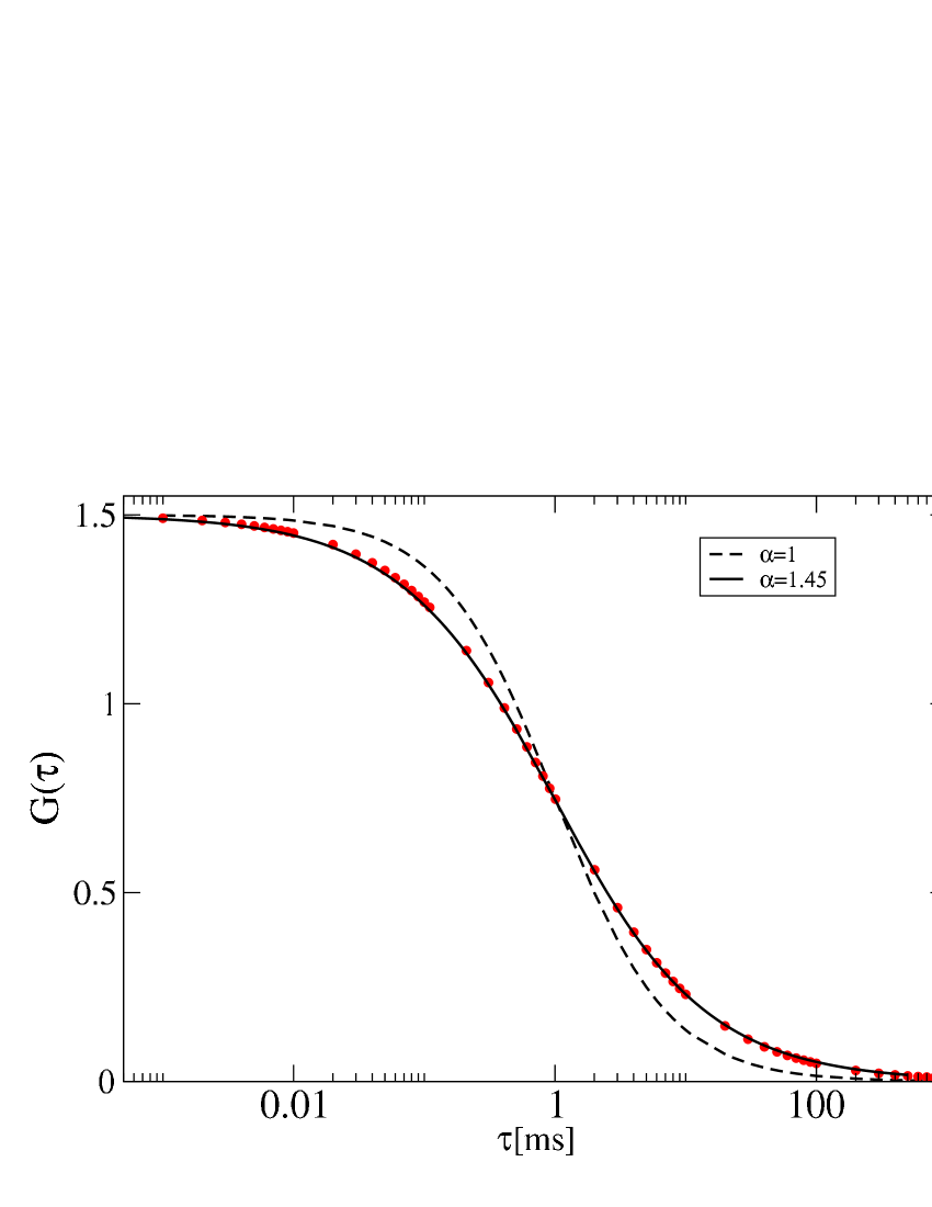
Figure 1: Fluorescence correlation spectrum. Experimental data (black dots) from Schwille et al, Fig.X in Webb , showing the fluorescence correlation intensity of lipid molecules diffusing in the plasma membrane of rat cells (vertical axis: intensity normalized values; horizontal axis: time in a.u.). The solid curve is the best-fit of the theoretical spectrum (52). For comparison the dashed curve shows the best-fit Gaussian profile (46).

References

• (1) A. Einstein, Ann. d. Phys., 17, 549 (1905).
• (2) I. Golding and E.C. Cox, Phys. Rev. Lett., 96, 098102 (2006).
• (3) T. Fujiwara et al., J. Cell Biol., 157, 1071 (2002).
• (4) T. Sanchez et al., Nature, 491, 431 (2012).
• (5) K.M. Douglass, S. Sukhov and A. Dogariu, Nature Photon., 6, 834 (2012).
• (6) I. M. Sokolov, J. Klafter and A. Blumen, Physics Today, 55, 48 (2002).
• (7) R. Metzler and J. Klafter, Phys. Rep., 339 (2000).
• (8) E. Barkai, Y. Garini and R. Metzler, Physics Today, 65, 29 (2012).
• (9) S. Abe, Phys. Rev. E , 88, 022142 (2013).
• (10) K. L. Sebastian, J. Phys. A, 28, 43054311 (1995).
• (11) I. Calvo and R. Sanchez, J. Phys. A, 41, 282002 (2008).
• (12) J. P. Boon and J. F. Lutsko, EuroPhys. Lett. , 80, 60006 (2007).
• (13) J. F. Lutsko and J. P. Boon, Phys. Rev. E , 77, 051103 (2008).
• (14) J. F. Lutsko and J. P. Boon, Phys. Rev. E , 88, 022108 (2013).
• (15) A phenomenological version of the nonlinear diffusion equation was first proposed by M. Muskat, The Flow of Homogeneous Fluids through Porous Media (McGrawHill, New York, 1937).
• (16) P. Schwille and E. Haustein, Fluorescence Correlation Spectroscopy, published in Biophysics Textbook Online (BTOL, 2007).
• (17) E.L. Elson, Biophys. Journal, 101, 2855 (2011).
• (18) P. Schwille, J. Korlach and W.W. Webb, Cytometry, 36, 176 (1999).