Inferring unobserved multistrain epidemic sub-populations using synchronization dynamics

Abstract

A new method is proposed to infer unobserved epidemic sub-populations by exploiting the synchronization properties of multistrain epidemic models. A model for dengue fever is driven by simulated data from secondary infective populations. Primary infective populations in the driven system synchronize to the correct values from the driver system. Most hospital cases of dengue are secondary infections, so this method provides a way to deduce unobserved primary infection levels. We derive center manifold equations that relate the driven system to the driver system and thus motivate the use of synchronization to predict unobserved primary infectives. Synchronization stability between primary and secondary infections is demonstrated through numerical measurements of conditional Lyapunov exponents and through time series simulations.

1 Introduction

Understanding spread of disease requires both observational data and mathematical modeling of some class or form (Anderson and May, 1991). However, much of the measured data is quite limited in that it is observed only once during typically short time intervals and typically is non-stationary. In many instances of observed disease spread, only case numbers per unit time are measured. As a result, even for simple, well known diseases, it is difficult to reconcile the models with the data.

An important component of epidemic modeling that cannot be reconciled with data are those individuals required to complete the disease path from susceptible to observed infected, which may consist of asymptomatic, individuals. Typically, intermittent stages along the disease path in between susceptible and infected cannot be measured directly. For example, in childhood diseases, certain susceptible individuals may have come in contact with someone who is infectious, but the resulting infected individual remains latent for a period of time. Sub-populations of such intermittent states are typically not observed directly, and must be inferred (Forgoston and Schwartz, 2013).

Alternative geometric modeling approaches to understanding epidemic spread have been examined using time series analysis from spatio-temporal case observations. Tools from nonlinear time series analysis using embedding theory have been applied to measles data (Schaffer et al., 1993; Blarer and Doebeli, 1999) to examine chaotic-like predictability of case history in the short term.

Another time series method of analysis for epidemic spread is that of Time-series Susceptible-Infected-Recovered (TSIR) modeling (Bjornstad et al., 2002). Local fits of time-series data generate measures of local reproductive rates of infection. For childhood diseases, the main assumption is that in the pre-vaccine years, all newborns introduced into the population as susceptible individuals become infected. However, the model excludes any latency period of infection, since it only considers models of SIR type. Therefore, the model does not predict time variations in the latent sub-population.

In general, since epidemic data is limited, detailed modeling of disease spread is required and thus is widespread. Connections of data with full models which are higher dimensional are difficult since there may exist many unobserved sub-populations along the disease path. High dimensional coupled patch models of cities have limited data time series when compared to the large simulation model dimension. Such limited data sets imply the need for accurate lower dimensional models to reduce the number of unknown parameters. Latency of infection, which introduces a series of exposed classes approximating mean delay times, is one example that generates high dimensional models. However, it is known rigorously that the dynamics in higher dimensional deterministic models often relaxes asymptotically onto lower dimensional hyper-surfaces, or center manifolds (Schwartz and Smith, 1983; Shaw et al., 2007). The advantage in doing center manifold reductions is that if one can only observe certain components of a disease, then it is possible to explicitly construct a function that relates the unobserved components (such as latency, or asymptomatic infections) to those explicitly measured or observed. Such a relationship, in which unobserved sub-populations are related dynamically to populations of disease that are measured, is closely aligned to synchronization of coupled systems.

Synchronization has frequently been studied in driver/driven dynamical systems (also called transmitter/receiver systems), in which information is transmitted unidirectionally from the driver to the driven system (Boccaletti et al., 2002). Some studies have focused on controlling parameters in the driven system until synchronization with the driver is achieved, as a way of determining unknown parameters in the driver system (Parlitz et al., 1996; Dedieu and Ogorzalek, 1997; Chen and Lü, 2002; Huang and Lin, 2013). When the systems are synchronized, observation of the driven system also allows unobserved variables from the driver system to be observed (Dedieu and Ogorzalek, 1997). In this paper, we propose a similar approach to determine unobserved quantities during an epidemic. The driver will be an observed time series, such as infection prevalence.

Our proposed method to infer unobserved epidemic compartments differs from previous approaches because we exploit synchronization dynamics rather than using statistical inference techniques. Previous studies focus more on integrating over or otherwise accounting for uncertainty in unknown compartments (Gibson et al., 2004; Lekone and Finkenstädt, 2006). However, it is frequently seen in epidemic models that the dynamics approach a lower dimensional center manifold. Examples include susceptible-exposed-infected-recovered (SEIR) models (Forgoston et al., 2009; Forgoston and Schwartz, 2013) and multistrain models for dengue fever (Shaw et al., 2007). Such results suggest that full information about an epidemic system is not needed, and variables that are more important to the dynamics can be used to deduce other, unknown variables.

We illustrate with a simple example for which it can be shown analytically that driving a system of unknown compartments with values from known compartments will result in convergence to the correct values for the unknown compartments. Consider a susceptible-infected-recovered (SIR) epidemic in a population with susceptible, infected, and recovered fractions $s(t)$, $i(t)$, and $r(t)$, respectively; birth and death rate $\mu$; contact rate $\beta$; and recovery rate $\sigma$. Suppose that the population dynamics is described by the system

$$\dot{s}=\mu-\beta si-\mu s$$ (1a)

$$\dot{i}=\beta si-\sigma i-\mu i$$ (1b)

$$\dot{r}=\sigma i-\mu r$$ (1c)

If a time series of the infected fraction $i(t)$ is known (e.g., from public health reporting) but the remaining compartments are unobserved, the susceptible fraction can be determined by driving a new differential equation with the known $i(t)$ as follows. Let $s_{d}(t)$ be the driven variable that we hope will reproduce the correct susceptible fraction, and evolve it according to

$$\dot{s}_{d}=\mu-\beta s_{d}i-\mu s_{d}.$$ (2)

The difference between $s$ and $s_{d}$, $\xi=s-s_{d}$, obeys

$$\dot{\xi}=-(\beta i+\mu)\xi.$$ (3)

Because $\beta i+\mu>0$ for all $t>0$, $\xi$ will approach 0 and $s_{d}$ will approach $s$ in the long time limit. Thus, given a sufficiently long time series for $i(t)$, the unknown susceptible levels can be determined for the latter part of the time series.

The application we will study here is a multistrain model for dengue fever (Schwartz et al., 2005). Dengue is a mosquito-borne disease with four co-circulating serotypes. In previous observations, secondary infections led to more severe illness and constituted the majority of dengue hospital cases (e.g., Nisalak et al. (2003)), so it is plausible that one may have data about secondary infections and want to deduce other asymptomatic quantities such as primary infective levels. It has been shown (Shaw et al., 2007) that the dynamics of this dengue model lie on a lower dimensional center manifold. In particular, peaks in primary and secondary infective levels are observed to coincide (Schwartz et al., 2005). However, the equations for secondary infectives derived in Shaw et al. (2007) require knowledge of susceptible and recovered compartments in addition to primary infectives. In this paper, we will show that primary infective levels can be determined by driving a system of equations with known secondary infective time series. Such a system has the practical value of using real measured data to extract unobserved compartments.

In Section 2, we review the multistrain model for dengue that will be used in this study. Section 3 presents center manifold analysis showing the relationship between driven and driver variables. Numerical results are presented in Section 4 demonstrating the efficacy of the proposed method, and Section 5 concludes the article.

2 The Two-Serotype Model

We begin by describing the compartmental multistrain disease model found in Schwartz et al. (2005), studying only two co-circulating serotypes for simplicity, but we remark that we expect the results to hold for arbitrary numbers of strains. We assume that a given population may be divided into the following classes that evolve in time:

1. Susceptible class $s(t)$ consists of the fraction of the total population that is susceptible to all serotypes.

2. Primary infectious classes $x_{i}(t)$ consist of the fraction of the total population that is infected with serotype $i$ and is capable of transmitting serotype $i$ to susceptible individuals.

3. Primary recovered classes $r_{i}(t)$ consist of the fraction of the total population that has recovered from being infected with serotype $i$.

4. Secondary infectious classes $x_{ij}(t)$ consist of the fraction of the total population that is currently infected with serotype $j$, but previously was infected with serotype $i$, where $i\neq j$.

In this model, susceptible individuals may develop a primary infection from either of the two serotypes. Upon recovering, the individual is immune to the strain that caused the primary infection. However, the individual may develop a secondary infection from the second serotype. The infectiousness of this secondary infection can be increased through an antibody-dependent enhancement factor. Upon recovering from the secondary infection, the individual is immune to both serotypes. A flow diagram for this model is given in Fig. 1.

Figure 1: Flow diagram for a multistrain disease model with two co-circulating serotypes (Schwartz et al., 2005). Included is the possibility of enhancing the secondary infectiousness through an antibody-dependent enhancement factor $\phi$.

The governing equations for the two serotype multistrain disease model are

$$\dot{s}=\mu-\beta s(x_{1}+x_{2}+\phi(x_{21}+x_{12})),$$ (4a)

$$\dot{x}_{1}=\beta s(x_{1}+\phi x_{21})-\sigma x_{1},$$ (4b)

$$\dot{x}_{2}=\beta s(x_{2}+\phi x_{12})-\sigma x_{2},$$ (4c)

$$\dot{r}_{1}=\sigma x_{1}-\beta r_{1}(x_{2}+\phi x_{12}),$$ (4d)

$$\dot{r}_{2}=\sigma x_{2}-\beta r_{2}(x_{1}+\phi x_{21}),$$ (4e)

$$\dot{x}_{21}=\beta r_{2}(x_{1}+\phi x_{21})-\sigma x_{21},$$ (4f)

$$\dot{x}_{12}=\beta r_{1}(x_{2}+\phi x_{12})-\sigma x_{12},$$ (4g)

where $\mu$ represents a constant birth rate, $\beta$ is the contact rate, $\phi$ is a constant that determines the antibody-dependent enhancement (ADE), and $\sigma$ is the rate of recovery, so that $1/\sigma$ is the mean infectious period. Although the contact rate $\beta$ could be given by a time-dependent function (e.g. due to seasonal fluctuations in the mosquito vector population), for simplicity, we assume $\beta$ to be constant. Unlike single strain models of $SIR$ type with constant contact rate, Eqs. (4a)-(4g) possess a range of $\phi$ where the endemic equilibrium is unstable.

Rates of infection due to primary infectious individuals have the form $\beta sx_{i}$, as found in a classical SIR epidemiological model. However, rates of infection due to secondary infectious individuals are weighted by the ADE parameter $\phi$, and have the form $\beta\phi sx_{ij}$. If $\phi=1$, then there is no antibody-dependent enhancement, and the primary and secondary infectious individuals are equally infectious. If $\phi=2$, then secondary infectious individuals are twice as infectious as primary infectious individuals, and so forth. As long as $\phi>1$ the nonlinear terms involving secondary infectious individuals will contain an antibody-dependent enhancement factor.

Throughout this article, we use the following parameter values: $\mu=0.02$(years)^-1, $\beta=200$(years)^-1, $\phi=3$(years)^-1, and $\sigma=50$(years)^-1. These disease parameters are consistent with estimates previously used in modeling dengue fever and are summarized in Table 1. In particular, the contact rate $\beta$ corresponds to a reproductive rate of infection $R_{0}$ of 3.2-4.8, which is consistent with estimates found in Ferguson et al. (1999) and Nagao and Koelle (2008).

The antibody-dependent enhancement parameter $\phi$ is selected to put the system in the chaotic regime in which the strains are desynchronized, which is thought to be the biologically relevant dynamics (c.f. Cummings et al. (2005); Shaw et al. (2007)). Dengue has four serotypes, but we model only two here for simplicity. The dynamics are similar for two and four serotypes, although there are shifts in the locations of bifurcation points and thus of realistic $\phi$ values (Billings et al., 2007). We anticipate that all the qualitative results of this paper will hold for more realistic four-serotype models.

Table 1: Model parameters.

Parameter	Value	Reference
$\mu$, birth rate, years-1	$\sim 0.02$	Ferguson et al. (1999)
$\beta$, transmission coefficient, years-1	$\sim 200$	Ferguson et al. (1999)
$\phi$, ADE parameter, years-1	$\geq 1$	Schwartz et al. (2005)
$\sigma$, recovery rate, years-1	$50$	Rigau-Perez et al. (1998)
$n$, number of strains	$2$	-

It should be noted that mortality terms have been omitted from Eqs. (4a)-(4g). In the analysis that follows, it is useful to analytically determine the endemic steady state. This equilibrium state is not easy to find analytically when mortality terms are included, but this state is close to the one found when all mortality occurs after recovery from infection with two serotypes, and the mortality rate of the other compartments is $\mu_{m}=0$. Previous work (Shaw et al., 2007) has shown that the dynamics with $\mu_{m}=0$ are qualitatively similar to the dynamics (and have the same bifurcation structure) when the mortality rate $\mu_{m}$ is equal to the value of the birth rate $\mu=0.02$ used in this article. Furthermore, the $\mu_{m}=0$ assumption is physically reasonable since the mortality rate for dengue is low and the average age at infection is believed to be young (Nisalak et al., 2003; Shaw et al., 2007)

The governing equations for the two serotype multistrain disease subsystem that are driven by the secondary infectious individuals of Eqs. (4a)-(4g) are

$$\dot{s}_{d}=\mu-\beta s_{d}(x_{d1}+x_{d2}+\phi(x_{21}+x_{12})),$$ (5a)

$$\dot{x}_{1d}=\beta s_{d}(x_{1d}+\phi x_{21})-\sigma x_{1d},$$ (5b)

$$\dot{x}_{2d}=\beta s_{d}(x_{2d}+\phi x_{12})-\sigma x_{2d},$$ (5c)

$$\dot{r}_{1d}=\sigma x_{1d}-\beta r_{1d}(x_{2d}+\phi x_{12}),$$ (5d)

$$\dot{r}_{2d}=\sigma x_{2d}-\beta r_{2d}(x_{1d}+\phi x_{21}),$$ (5e)

where the subscript $d$ signifies that the variable is being driven. As before, $\mu$ represents a constant birth rate, $\beta$ is the contact rate, $\phi$ is a constant that determines the antibody-dependent enhancement (ADE), and $\sigma$ is the rate of recovery, with parameter values shown in Table 1.

Since $r_{1d}$ and $r_{2d}$ are decoupled from Eqs. (4a)-(5c), the center manifold analysis of the following section will be performed using the simpler 10-dimensional system given by Eqs. (4a)-(5c).

3 Center Manifold Analysis

We will reduce the dimension of the system given by Eqs. (4a)-(5c) using the center manifold of the system. The analysis begins by determining the endemic equilibrium state of the system. It is given as

$$(s_{0},x_{i,0},r_{i,0},x_{ij,0},s_{d,0},x_{id,0})=\left(\frac{\sigma}{\beta(1+\phi)},\frac{\mu}{2\sigma},\frac{\sigma}{\beta(1+\phi)},\frac{\mu}{2\sigma},\frac{\sigma}{\beta(1+\phi)},\frac{\mu}{2\sigma}\right)$$ (6)

for all $i,j$.

A general nonlinear system may be transformed so that the system’s linear part has a block diagonal form consisting of three matrix blocks. The first matrix block will possess eigenvalues with positive real part; the second matrix block will possess eigenvalues with negative real part; and the third matrix block will possess eigenvalues with zero real part. These three matrix blocks are respectively associated with the unstable eigenspace, the stable eigenspace, and the center eigenspace. If there are no eigenvalues with positive real part, then the orbits will rapidly decay to the center eigenspace.

Equations (4a)-(5c) cannot be written in a block diagonal form with one matrix block possessing eigenvalues with negative real part and the other matrix block possessing eigenvalues with zero real part. Even though it is possible to construct a center manifold from a system not in separated block form (Chicone and Latushkin, 1997), it is much easier to apply the center manifold theory to a system with separated stable and center directions. Therefore, we transform the original system given by Eqs. (4a)-(5c) to a new system of equations that will have the eigenvalue structure that is needed to apply center manifold theory. The theory allows one to find an invariant center manifold that passes through a fixed point and to which one can restrict the new transformed system.

3.1 Transformation of the Two-Serotype Model

To ease the analysis, we define a new set of variables, $\bar{s}$, $\bar{x}_{i}$, $\bar{r}_{i}$, $\bar{x}_{ij}$, $\bar{s}_{d}$, and $\bar{x}_{id}$ for all $i,j$ as $\bar{s}(t)=s(t)-s_{0}$, $\bar{x}_{i}(t)=x_{i}(t)-x_{i,0}$, $\bar{r}_{i}(t)=r(t)-r_{i,0}$, $\bar{x}_{ij}(t)=x_{ij}(t)-x_{ij,0}$, $\bar{s}_{d}(t)=s_{d}(t)-s_{d,0}$, $\bar{x}_{id}(t)=x_{id}(t)-x_{id,0}$. These new variables are substituted into Eqs. (4a)-(5c).

Then, treating $\mu$ as a small parameter, we rescale time by letting $t=\mu\tau$. We may then introduce the following rescaled parameters: $\beta=\beta_{0}/\mu$ and $\sigma=\sigma_{0}/\mu$, where $\beta_{0}$ and $\sigma_{0}$ are $\mathcal{O}(1)$. The inclusion of the parameter $\mu$ as a new state variable means that the terms in our rescaled system which contain $\mu$ are now nonlinear terms. Furthermore, the system is augmented with the auxiliary equation $\frac{d\mu}{d\tau}=0$. The addition of this auxiliary equation contributes an extra simple zero eigenvalue to the system and adds one new center direction that has trivial dynamics. The shifted and rescaled, augmented system of equations now have the endemic fixed point located at the origin and are provided in Appendix A.

The Jacobian of these shifted and rescaled equations (Eqs. (21a)-(21k)) is computed to zeroth-order in $\mu$ and is evaluated at the origin. Ignoring the $\mu$ components, the Jacobian has only eight linearly independent eigenvectors. Therefore, the Jacobian is not diagonalizable. However, it is possible to transform Eqs. (21a)-(21j) to a block diagonal form with a separated eigenvalue structure. As mentioned previously, this block structure makes the center manifold analysis easier. We use a transformation matrix, ${\bf P}$, consisting of the eight linearly independent eigenvectors of the Jacobian along with two other vectors chosen to be linearly independent. There are many choices for these ninth and tenth vectors; our choice is predicated on keeping the vectors as simple as possible. This transformation matrix is given as follows:

$${\bf P}=\left[\begin{array}[]{cccccccccc}0&0&0&0&1&0&0&0&0&0\\ -\phi&0&0&0&0&1&0&0&0&0\\ 0&-\phi&0&0&0&0&1&0&0&0\\ \phi&0&0&0&0&0&0&1&0&0\\ 0&\phi&0&0&0&0&0&0&1&0\\ 1&0&0&0&0&1&0&0&0&0\\ 0&1&0&0&0&0&1&0&0&0\\ 0&0&1&0&0&0&0&0&0&1\\ -\phi&0&\phi&-1&0&1&0&0&0&0\\ 0&-\phi&0&1&0&0&1&0&0&0\\ \end{array}\right].$$ (7)

Using the fact that $(\bar{s},\bar{x}_{1},\bar{x}_{2},\bar{r}_{1},\bar{r}_{2},\bar{x}_{21},\bar{x}_{12},\bar{s}_{d},\bar{x}_{1d},\bar{x}_{2d})^{T}={\bf P}\cdot{\bf W}^{T}$, where ${\bf W}=(W_{1},W_{2},W_{3},W_{4},W_{5},W_{6},W_{7},W_{8},W_{9},W_{10})$, then the transformation matrix leads to the definition of new variables, $W_{i}$, $i=1\ldots 10$ that can be found in Appendix B. The application of the transformation matrix to Eqs. (21a)-(21j) leads to a set of transformed evolution equations that are found in Appendix C.

3.2 Application of the Center Manifold Theory

The Jacobian of Eqs. (23a)-(23k) to zeroth-order in $\mu$ and evaluated at the origin is

$$\left[\begin{array}[]{cccc|cccccc}-\sigma_{0}&0&0&0&0&0&0&0&0&0\\ 0&-\sigma_{0}&0&0&0&0&0&0&0&0\\ 0&0&-\frac{\phi\sigma_{0}}{1+\phi}&0&0&0&0&0&0&0\\ 0&0&0&-\frac{\phi\sigma_{0}}{1+\phi}&0&0&0&0&0&0\\ \hline\cr 0&0&0&0&0&-\sigma_{0}&-\sigma_{0}&0&0&0\\ 0&0&0&0&0&0&0&0&0&0\\ 0&0&0&0&0&0&0&0&0&0\\ 0&0&0&0&0&\sigma_{0}&-\sigma_{0}&0&0&0\\ 0&0&0&0&0&-\sigma_{0}&\sigma_{0}&0&0&0\\ 0&0&0&0&0&-\sigma_{0}&-\sigma_{0}&0&0&0\\ \end{array}\right],$$ (8)

which shows that Eqs. (23a)-(23k) may be rewritten in the form

$$\frac{d{\bf x}}{d\tau}={\bf A}{\bf x}+{\bf f}({\bf x},{\bf y},\mu),$$ (9)

$$\frac{d{\bf y}}{d\tau}={\bf B}{\bf y}+{\bf g}({\bf x},{\bf y},\mu),$$ (10)

$$\frac{d\mu}{d\tau}=0,$$ (11)

where ${\bf x}=(W_{1},W_{2},W_{3},W_{4})$, ${\bf y}=(W_{5},W_{6},W_{7},W_{8},W_{9},W_{10})$, ${\bf A}$ is a constant matrix with eigenvalues that have negative real parts, ${\bf B}$ is a constant matrix with eigenvalues that have zero real parts, and ${\bf f}$ and ${\bf g}$ are nonlinear functions in ${\bf x}$, ${\bf y}$ and $\mu$. In particular, ${\bf A}$ is the upper left block matrix of Eq. (8), while ${\bf B}$ is the lower right block matrix of Eq. (8).

Therefore, this new system of equations, which is an exact transformation of Eqs. (4a)-(5c), will rapidly collapse onto a lower-dimensional manifold given by center manifold theory (Carr, 1981; Chicone and Latushkin, 1997; Duan et al., 2003). Furthermore, the lower dimensional center manifold is given by

$$W_{i}=h_{i}(\bm{y},\mu)$$ (12)

where $h_{i}$, $i=1\ldots 4$ are unknown functions.

Substitution of the center manifold functions $W_{i}=h_{i}$ given by Eq. (12) into the transformed evolution equations given in Appendix C leads to the center manifold condition given in Appendix D.

In general, it is not possible to solve the center manifold condition for the four unknown functions $h_{i}(\bm{y},\mu)$, $i=1\ldots 4$. Therefore, a Taylor series expansion of $h_{i}(\bm{y},\mu)$, $i=1\ldots 4$ in $\bm{y}$ and $\mu$ is substituted into the four equations that comprise the center manifold condition (Eqs. (24a)-(24d)). The unknown coefficients are determined by equating terms of the same order, and the center manifold equations are found to be

$$W_{1}= \frac{-\beta_{0}}{\sigma_{0}}W_{5}W_{6}-2\frac{\beta_{0}}{\sigma_{0}}W_{6}W_{7}+\frac{\beta_{0}}{\sigma_{0}}W_{6}W_{9}+\mathcal{O}(\epsilon^{3}),$$ (13a)

$$W_{2}= \frac{-\beta_{0}}{\sigma_{0}}W_{5}W_{7}-2\frac{\beta_{0}}{\sigma_{0}}W_{6}W_{7}+\frac{\beta_{0}}{\sigma_{0}}W_{7}W_{8}+\mathcal{O}(\epsilon^{3}),$$ (13b)

$$W_{3}= -\frac{\beta_{0}(1+\phi)^{2}}{\phi^{2}\sigma_{0}}W_{5}W_{6}-\frac{\beta_{0}(1+\phi)^{2}}{\phi^{2}\sigma_{0}}W_{5}W_{7}+\frac{\beta_{0}(1+\phi)^{2}}{\phi^{2}\sigma_{0}}W_{6}W_{10}$$

$$+\frac{\beta_{0}(1+\phi)^{2}}{\phi^{2}\sigma_{0}}W_{7}W_{10}+\mathcal{O}(\epsilon^{3}),$$ (13c)

$$W_{4}= -\frac{\beta_{0}(1+\phi)^{2}}{\phi\sigma_{0}}W_{5}W_{7}+\frac{\beta_{0}(1+\phi)^{2}}{\phi\sigma_{0}}W_{7}W_{10}+\mathcal{O}(\epsilon^{3}),$$ (13d)

where $\epsilon=|(W_{5},W_{6},W_{7},W_{8},W_{9},W_{10},\mu)|$ so that $\epsilon$ provides a count of the number of $W_{5}$, $W_{6}$, $W_{7}$, $W_{8}$, $W_{9}$, $W_{10}$, and $\mu$ factors in any one term. It is worth noting that the center manifold equations may equivalently be found using a normal form coordinate transform. Details of the method can be found in Roberts (2008) and application to epidemic models can be found in Forgoston et al. (2009) and Forgoston and Schwartz (2013)

Using the relations between $W_{i}$ variables and the “barred” variables given by Eq. (22), Eqs. (13a)-(13d) can be equivalently written as follows:

$$\sigma_{0}(\bar{x}_{1}-\bar{x}_{21})=\beta_{0}(\bar{x}_{1}+\phi\bar{x}_{21})\left[\bar{s}-\bar{r}_{2}+\frac{3\phi}{(1+\phi)}\bar{x}_{12}+\frac{2-\phi}{(1+\phi)}\bar{x}_{2}\right],$$ (14a)

$$\sigma_{0}(\bar{x}_{2}-\bar{x}_{12})=\beta_{0}(\bar{x}_{2}+\phi\bar{x}_{12})\left[\bar{s}-\bar{r}_{1}+\frac{3\phi}{(1+\phi)}\bar{x}_{21}+\frac{2-\phi}{(1+\phi)}\bar{x}_{1}\right],$$ (14b)

$$\sigma_{0}\left[\bar{x}_{d1}+\bar{x}_{d2}-\bar{x}_{1}-\bar{x}_{2}\right]=\frac{\beta_{0}(1+\phi)^{2}}{\phi^{2}}\left[\bar{x}_{1}+\bar{x}_{2}-\bar{x}_{d1}-\bar{x}_{d2}-\phi\bar{s}+\phi\bar{s}_{d}\right]\times$$

$$\hskip 113.81102pt\left[\frac{\bar{x}_{1}+\bar{x}_{2}+\phi\bar{x}_{12}+\phi\bar{x}_{21}}{(1+\phi)}\right],$$ (14c)

$$\sigma_{0}\left[\bar{x}_{d2}-\bar{x}_{2}\right]=\frac{\beta_{0}(1+\phi)^{2}}{\phi^{2}}\left[\bar{x}_{1}+\bar{x}_{2}-\bar{x}_{d1}-\bar{x}_{d2}-\phi\bar{s}+\phi\bar{s}_{d}\right]\times\left[\frac{\bar{x}_{2}+\phi\bar{x}_{12}}{(1+\phi)}\right].$$ (14d)

It is possible to simplify Eq. (14c) by substituting Eq. (14d) into Eq. (14c). The resulting simplified Eq. (14c) is

$$\sigma_{0}\left[\bar{x}_{d1}-\bar{x}_{1}\right]=\frac{\beta_{0}(1+\phi)^{2}}{\phi^{2}}\left[\bar{x}_{1}+\bar{x}_{2}-\bar{x}_{d1}-\bar{x}_{d2}-\phi\bar{s}+\phi\bar{s}_{d}\right]\times\left[\frac{\bar{x}_{1}+\phi\bar{x}_{21}}{(1+\phi)}\right].$$ (15)

Solving Eqs. (14a)-(14b) for $\bar{x}_{1}$, $\bar{x}_{2}$ leads to the following approximation for the invariant manifold onto which the driver system collapses:

$$\bar{x}_{1}=\frac{\sigma_{0}\bar{x}_{21}+\beta_{0}\phi\bar{x}_{21}\left[\bar{s}-\bar{r}_{2}+\frac{2-\phi}{1+\phi}\bar{x}_{2}+\frac{3\phi}{1+\phi}\bar{x}_{12}\right]}{\sigma_{0}-\beta_{0}\left[\bar{s}-\bar{r}_{2}+\frac{2-\phi}{1+\phi}\bar{x}_{2}+\frac{3\phi}{1+\phi}\bar{x}_{12}\right]}$$ (16a)

$$\bar{x}_{2}=\frac{\sigma_{0}\bar{x}_{12}+\beta_{0}\phi\bar{x}_{12}\left[\bar{s}-\bar{r}_{1}+\frac{2-\phi}{1+\phi}\bar{x}_{1}+\frac{3\phi}{1+\phi}\bar{x}_{21}\right]}{\sigma_{0}-\beta_{0}\left[\bar{s}-\bar{r}_{1}+\frac{2-\phi}{1+\phi}\bar{x}_{1}+\frac{3\phi}{1+\phi}\bar{x}_{21}\right]}.$$ (16b)

This invariant manifold was found previously in Shaw et al. (2007) and represents the close relationship of primary infectives and secondary infectives.

Similarly, solving the simplified Eq. (14c) given by Eq. (15) and Eqs. (14d) simultaneously for $\bar{x}_{d1}$ and $\bar{x}_{d2}$ leads to an approximate invariant manifold for the driven primary infectives expressed almost entirely in terms of driver system variables:

$$\bar{x}_{d1}=\frac{\left(\sigma_{0}\bar{x}_{1}\left(1+\phi\right)+\Gamma\left[\bar{x}_{1}\left(\bar{x}_{1}+\bar{x}_{2}+\phi\left(\bar{x}_{12}+\bar{x}_{21}\right)\right)+\phi\left(\bar{s}_{d}-\bar{s}\right)\left(\bar{x}_{1}+\phi\bar{x}_{21}\right)\right]\right)}{\sigma_{0}\left(1+\phi\right)+\Gamma\left(\bar{x}_{1}+\bar{x}_{2}+\phi\left(\bar{x}_{12}+\bar{x}_{21}\right)\right)}$$ (17a)

$$\bar{x}_{d2}=\frac{\left(\sigma_{0}\bar{x}_{2}\left(1+\phi\right)+\Gamma\left[\bar{x}_{2}\left(\bar{x}_{1}+\bar{x}_{2}+\phi\left(\bar{x}_{12}+\bar{x}_{21}\right)\right)+\phi\left(\bar{s}_{d}-\bar{s}\right)\left(\bar{x}_{2}+\phi\bar{x}_{12}\right)\right]\right)}{\sigma_{0}\left(1+\phi\right)+\Gamma\left(\bar{x}_{1}+\bar{x}_{2}+\phi\left(\bar{x}_{12}+\bar{x}_{21}\right)\right)}$$ (17b)

where $\Gamma=\frac{\beta_{0}\left(1+\phi\right)^{2}}{\phi^{2}}$. Although these equations do not prove that the driven system synchronizes to the driver system, they do indicate that the driven system rapidly approaches a manifold in which the driven primary infectives are strongly affected by the infectives in the driver system. We show in subsequent numerical simulations that the driven variables do in fact approach those in the driver system.

4 Results

4.1 Comparison of Solutions

The original equations in the shifted, barred variables (Eqs. (21a)-(21j)) are solved, and the values of the variables found on the right hand side of Eqs. (16a)-(17b) are substituted into Eqs. (16a)-(17b) to find the value of $\bar{x}_{1}$, $\bar{x}_{2}$, $\bar{x}_{d1}$, and $\bar{x}_{d2}$ given by the center manifold equations. After computing in the shifted variables, we shift back to the original variables.

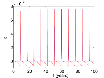
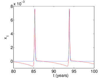
Figure 2: Plot of $x_{1}$ computed using the complete system of equations (blue) and the center manifold equation (red) for (a) $t=0$ to $t=100$, and (b) $t=80$ to $t=100$. Parameter values are given by $\mu=0.02$, $\sigma=50.0$, $\phi=3.0$, and $\beta=200.0$.

Figure 2(a) shows a comparison of $x_{1}$ found through computation of the complete system and found through computation using the center manifold equation. To show the agreement more clearly, Fig. 2(b) shows a portion of Fig. 2(a). The prediction for the primary infectives is occasionally negative since the center manifold equations involve $\bar{x}_{i}$ terms which represent infectives shifted from their fixed point. As discussed in Shaw et al. (2007), the predicted deviations may be large enough so that adding the fixed point $x_{i,0}$ results in a negative value for the $x_{i}$ terms. However, since the errors occur in regions where there is no epidemic outbreak, they are not of biological importance. Furthermore, one can see that the timing of the outbreaks predicted by the reduced system agrees well with the actual outbreak time of the complete system.

Figure 3(a) and (c) shows the comparison of $x_{d1}$ and $x_{d2}$ respectively found through computation of the complete system and found through computation using the center manifold equation. The agreement is perfect and is seen more clearly in Figs. 3(b) and (d) which show portion of Figs. 3(a) and (c) respectively.

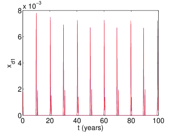
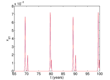
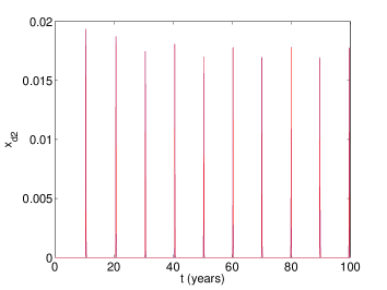
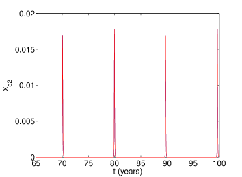
Figure 3: Plots of (a)-(b) $x_{d1}$ and (c)-(d) $x_{d2}$ computed using the complete system of equations (blue) and the center manifold equation (red) for (a) and (c) $t=0$ to $t=100$, and (b) and (d) $t=65$ to $t=100$. Parameter values are given by $\mu=0.02$, $\sigma=50.0$, $\phi=3.0$, and $\beta=200.0$.

4.2 Transverse Stability

To show that the driven system synchronizes with the full system for the components chosen, we can examine the transverse stability of the solution of the subsystem. That is, we examine the difference between the full vector field (the driver) and the subsystem. By computing the linear variational equations of the difference, we can find the conditional Lyapunov exponents for solutions near the subsystem.

To establish notation, we rewrite the components of the governing equations for the two serotype multistrain disease model as

$${\bf X}=[s,x_{1},x_{2}]^{T}\quad{\bf Y}=[r_{1},r_{2},x_{21},x_{12}]^{T},$$ (18)

where $T$ denotes the transpose. Additionally, we can rewrite the components of the governing equations for the two serotype multistrain disease subsystem that are driven by the secondary infectious individuals as

$${\bf Z}=[s_{d},x_{1d},x_{2d}]^{T}.$$ (19)

To write the system of equations we consider the split differential equations

$${\bf{\bf\dot{X}}=F_{1}(X,Y)}$$ (20a)

$${\bf{\bf\dot{Y}}=F_{2}(X,Y).}$$ (20b)

along with the subsystem

$${\bf{\bf\dot{Z}}=F_{1}(Z,Y)}.$$ (20c)

We would like ${\bf Z}(t)\rightarrow{\bf X}(t)$ in the asymptotic limit. Letting ${\bm{\xi}}={\bf X}-{\bf Z}$, one obtains the linear variation about ${\bf X}(t)$ given by ${\dot{\bm{\xi}}}={\bf F}_{1,x}({\bf X},{\bf Y}){\bm{\xi}}$. The Lyapunov exponents of the subsystem are the conditional Lyapunov exponents (CLE). Negative CLE provide a sufficient condition for the subsystem to converge, and are shown in Fig. 4.

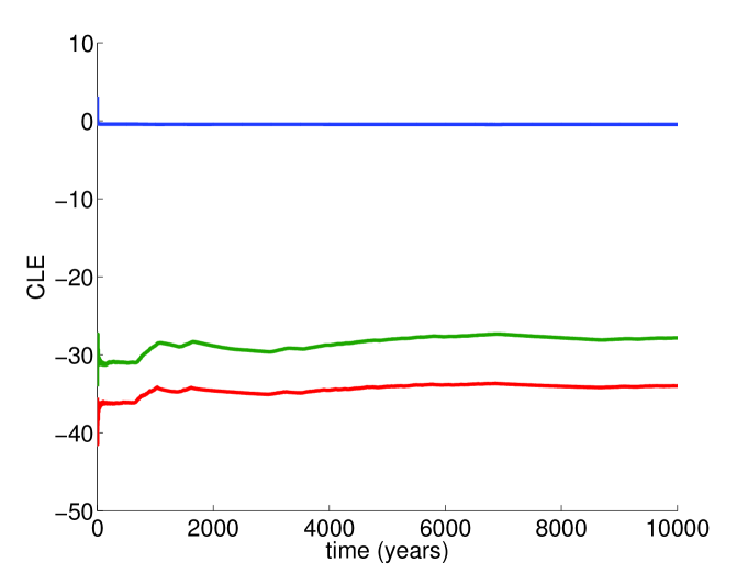
Figure 4: Time series of the conditional Lyapunov exponents. Parameter values are given by $\mu=0.02$, $\sigma=50.0$, $\phi=3.0$, and $\beta=200.0$. The initial condition for the driver system was a point on the chaotic attractor obtained by computing a long time series, and the initial condition for the driven system was a perturbation from the driver.

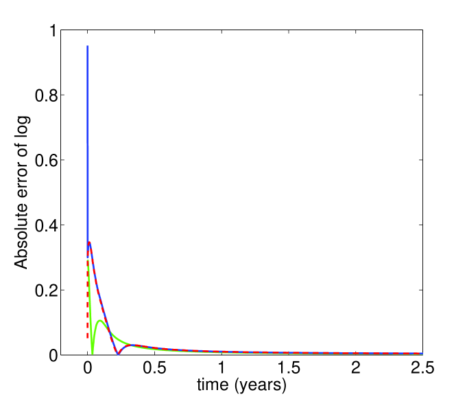
Figure 5: Absolute error in log variables for susceptibles and primary infectives versus time. Solid green: $|\log s_{d}-\log s|$, solid blue: $|\log x_{1d}-\log x_{1}|$, dashed red: $|\log x_{2d}-\log x_{2}|$. The initial condition for the driver system was a point on the chaotic attractor obtained by computing a long time series. The initial condition for the driven system was a random perturbation with mean 10% away from the driver system. Parameter values are the same as in Fig. 4.

In Fig. 5, we show a sample time series of the error between the driven and driver systems. Susceptibles and primary infectives in the driven system rapidly converge to the values found in the driver system. Even when the driven system is initially perturbed farther from the driver system, convergence occurs within a similar time period.

5 Conclusions

In this article, we considered a two serotype multistrain disease model in which susceptibles may develop a primary infection from either of the two serotypes and upon recovery become immune to the strain that caused the primary infection. However, the second serotype may cause a secondary infection. We also consider a two serotype multistrain disease subsystem that is driven by the secondary infectious individuals of the first model. By performing center manifold analysis, we can reduce the dimension of these driven and driver systems. In particular, we were able to analytically find an approximate invariant manifold for the driven primary infectives expressed almost entirely in terms of driver system variables. Numerical simulations demonstrate the excellent agreement between solutions of the original, higher-dimensional system and the lower-dimensional center manifold equations. We further demonstrated the driven system is synchronized with the complete system by examining the transverse stability of the subsystem solution.

In summary, we have developed a new method to determine unobserved epidemic sub-populations using synchronization properties of the epidemic model. As an application, it is known that the majority of dengue fever hospital cases are secondary infections Nisalak et al. (2003). Thus one may have information about secondary infections but not about primary infections. In driving a model using the known secondary infection data, the primary infective populations in the driven system synchronize to the correct values from the driver system. It is therefore possible to deduce unobserved primary infection levels in the population. It should be noted that this method probably works for other multistrain models, such as the dengue model in Bianco et al. (2009) in which we include temporary cross immunity immediately following a primary infection.

Future work includes the application of our method to real disease data. Before this can be performed, one would first have to perform the analysis in the presence of noise (i.e. the driver signal comes from a noisy system and/or has additional errors in it). Additionally, the theory will need to be applied to the situation when data is sampled discretely. Preliminary testing using discretely sampled data for the secondary infectives has shown that the technique can indeed recover primary infectives.

Appendix A Shifted, Rescaled, and Augmented System of Equations

The governing equations for the two serotype multistrain disease model and the subsystem driven by secondary infectious individuals are given by Eqs. (4a)-(5c). We define a new set of variables, $\bar{s}$, $\bar{x}_{i}$, $\bar{r}_{i}$, $\bar{x}_{ij}$, $\bar{s}_{d}$, and $\bar{x}_{id}$ for all $i,j$ as $\bar{s}(t)=s(t)-s_{0}$, $\bar{x}_{i}(t)=x_{i}(t)-x_{i,0}$, $\bar{r}_{i}(t)=r(t)-r_{i,0}$, $\bar{x}_{ij}(t)=x_{ij}(t)-x_{ij,0}$, $\bar{s}_{d}(t)=s_{d}(t)-s_{d,0}$, $\bar{x}_{id}(t)=x_{id}(t)-x_{id,0}$, and these new variables are substituted into Eqs. (4a)-(5c).

Then, treating $\mu$ as a small parameter, we rescale time by letting $t=\mu\tau$. We may then introduce the following rescaled parameters: $\beta=\beta_{0}/\mu$ and $\sigma=\sigma_{0}/\mu$, where $\beta_{0}$ and $\sigma_{0}$ are $\mathcal{O}(1)$. The inclusion of the parameter $\mu$ as a new state variable means that the terms in our rescaled system which contain $\mu$ are now nonlinear terms. Furthermore, the system is augmented with the auxiliary equation $\frac{d\mu}{d\tau}=0$. The addition of this auxiliary equation contributes an extra simple zero eigenvalue to the system and adds one new center direction that has trivial dynamics. The shifted and rescaled, augmented system of equations is given as

$$\frac{d\bar{s}}{d\tau}=\mu^{2}-\beta_{0}\left(\bar{s}+\frac{\sigma_{0}}{\beta_{0}(1+\phi)}\right)\left(\bar{x}_{1}+\bar{x}_{2}+\phi\left(\bar{x}_{21}+\bar{x}_{12}\right)+\frac{\mu^{2}(1+\phi)}{\sigma_{0}}\right),$$ (21a)

$$\frac{d\bar{x}_{1}}{d\tau}=\beta_{0}\left(\bar{s}+\frac{\sigma_{0}}{\beta_{0}(1+\phi)}\right)\left(\bar{x}_{1}+\phi\bar{x}_{21}+\frac{\mu^{2}(1+\phi)}{2\sigma_{0}}\right)-\sigma_{0}\left(\bar{x}_{1}+\frac{\mu^{2}}{2\sigma_{0}}\right),$$ (21b)

$$\frac{d\bar{x}_{2}}{d\tau}=\beta_{0}\left(\bar{s}+\frac{\sigma_{0}}{\beta_{0}(1+\phi)}\right)\left(\bar{x}_{2}+\phi\bar{x}_{12}+\frac{\mu^{2}(1+\phi)}{2\sigma_{0}}\right)-\sigma_{0}\left(\bar{x}_{2}+\frac{\mu^{2}}{2\sigma_{0}}\right),$$ (21c)

$$\frac{d\bar{r}_{1}}{d\tau}=\sigma_{0}\left(\bar{x}_{1}+\frac{\mu^{2}}{2\sigma_{0}}\right)-\beta_{0}\left(\bar{r}_{1}+\frac{\sigma_{0}}{\beta_{0}(1+\phi)}\right)\left(\bar{x}_{2}+\phi\bar{x}_{12}+\frac{\mu^{2}(1+\phi)}{2\sigma_{0}}\right),$$ (21d)

$$\frac{d\bar{r}_{2}}{d\tau}=\sigma_{0}\left(\bar{x}_{2}+\frac{\mu^{2}}{2\sigma_{0}}\right)-\beta_{0}\left(\bar{r}_{2}+\frac{\sigma_{0}}{\beta_{0}(1+\phi)}\right)\left(\bar{x}_{1}+\phi\bar{x}_{21}+\frac{\mu^{2}(1+\phi)}{2\sigma_{0}}\right),$$ (21e)

$$\frac{d\bar{x}_{21}}{d\tau}=\beta_{0}\left(\bar{r}_{2}+\frac{\sigma_{0}}{\beta_{0}(1+\phi)}\right)\left(\bar{x}_{1}+\phi\bar{x}_{21}+\frac{\mu^{2}(1+\phi)}{2\sigma_{0}}\right)-\sigma_{0}\left(\bar{x}_{21}+\frac{\mu^{2}}{2\sigma_{0}}\right),$$ (21f)

$$\frac{d\bar{x}_{12}}{d\tau}=\beta_{0}\left(\bar{r}_{1}+\frac{\sigma_{0}}{\beta_{0}(1+\phi)}\right)\left(\bar{x}_{2}+\phi\bar{x}_{12}+\frac{\mu^{2}(1+\phi)}{2\sigma_{0}}\right)-\sigma_{0}\left(\bar{x}_{12}+\frac{\mu^{2}}{2\sigma_{0}}\right),$$ (21g)

$$\frac{d\bar{s}_{d}}{d\tau}=\mu^{2}-\beta_{0}\left(\bar{s}_{d}+\frac{\sigma_{0}}{\beta_{0}(1+\phi)}\right)\left(\bar{x}_{1d}+\bar{x}_{2d}+\phi\left(\bar{x}_{21}+\bar{x}_{12}\right)+\frac{\mu^{2}(1+\phi)}{\sigma_{0}}\right),$$ (21h)

$$\frac{d\bar{x}_{1d}}{d\tau}=\beta_{0}\left(\bar{s}_{d}+\frac{\sigma_{0}}{\beta_{0}(1+\phi)}\right)\left(\bar{x}_{1d}+\phi\bar{x}_{21}+\frac{\mu^{2}(1+\phi)}{2\sigma_{0}}\right)-\sigma_{0}\left(\bar{x}_{1d}+\frac{\mu^{2}}{2\sigma_{0}}\right),$$ (21i)

$$\frac{d\bar{x}_{2d}}{d\tau}=\beta_{0}\left(\bar{s}_{d}+\frac{\sigma_{0}}{\beta_{0}(1+\phi)}\right)\left(\bar{x}_{2d}+\phi\bar{x}_{12}+\frac{\mu^{2}(1+\phi)}{2\sigma_{0}}\right)-\sigma_{0}\left(\bar{x}_{2d}+\frac{\mu^{2}}{2\sigma_{0}}\right),$$ (21j)

$$\frac{d\mu}{d\tau}=0,$$ (21k)

where the endemic fixed point is now located at the origin.

Appendix B Definition of New Variables

Using the fact that $(\bar{s},\bar{x}_{1},\bar{x}_{2},\bar{r}_{1},\bar{r}_{2},\bar{x}_{21},\bar{x}_{12},\bar{s}_{d},\bar{x}_{1d},\bar{x}_{2d})^{T}={\bf P}\cdot{\bf W}^{T}$, where ${\bf P}$ is given by Eq. (7) and ${\bf W}=(W_{1},W_{2},W_{3},W_{4},W_{5},W_{6},W_{7},W_{8},W_{9},W_{10})$, then the transformation matrix leads to the following definition of new variables, $W_{i}$, $i=1\ldots 10$:

$$\begin{split}&W_{1}=\frac{\bar{x}_{21}-\bar{x}_{1}}{1+\phi},\quad W_{2}=\frac{\bar{x}_{12}-\bar{x}_{2}}{1+\phi},\quad W_{3}=\frac{\bar{x}_{1d}+\bar{x}_{2d}-\bar{x}_{1}-\bar{x}_{2}}{\phi},\quad W_{4}=\bar{x}_{2d}-\bar{x}_{2},\\ &W_{5}=\bar{s},\quad W_{6}=\frac{\bar{x}_{1}+\phi\bar{x}_{21}}{1+\phi},\quad W_{7}=\frac{\bar{x}_{2}+\phi\bar{x}_{12}}{1+\phi},\quad W_{8}=\frac{\phi\bar{r}_{1}+\phi\bar{x}_{1}+\bar{r}_{1}-\phi\bar{x}_{21}}{1+\phi},\\ &W_{9}=\frac{\phi\bar{r}_{2}+\phi\bar{x}_{2}+\bar{r}_{2}-\phi\bar{x}_{12}}{1+\phi},\quad W_{10}=\frac{\phi\bar{s}_{d}-\bar{x}_{1d}-\bar{x}_{2d}+\bar{x}_{1}+\bar{x}_{2}}{\phi}.\end{split}$$ (22)

Appendix C Transformed Evolution Equations

The application of the transformation matrix ${\bf P}$ given by Eq. (7) to Eqs. (21a)-(21j) leads to the following set of transformed evolution equations:

$$\frac{dW_{1}}{d\tau}=\beta_{0}\left(W_{6}+\frac{\mu^{2}}{2\sigma_{0}}\right)\left(W_{9}+\phi W_{2}-W_{5}\right)-\sigma_{0}W_{1},$$ (23a)

$$\frac{dW_{2}}{d\tau}=\beta_{0}\left(W_{7}+\frac{\mu^{2}}{2\sigma_{0}}\right)\left(W_{8}+\phi W_{1}-W_{5}\right)-\sigma_{0}W_{2},$$ (23b)

$$\frac{dW_{3}}{d\tau}=W_{3}\left(\beta_{0}\left(W_{3}+W_{10}\right)-\frac{\sigma_{0}\phi}{1+\phi}\right)$$

$$\hskip 28.45274pt+\frac{\beta_{0}\left(1+\phi\right)}{\phi}\left(W_{6}+W_{7}+\frac{\mu^{2}}{\sigma_{0}}\right)\left(W_{3}+W_{10}-W_{5}\right),$$ (23c)

$$\frac{dW_{4}}{d\tau}=\left(\beta_{0}\left(W_{3}+W_{10}\right)-\frac{\sigma_{0}\phi}{1+\phi}\right)W_{4}$$

$$\hskip 28.45274pt+\beta_{0}\left(W_{3}+W_{10}-W_{5}\right)\left(\left(1+\phi\right)W_{7}+\frac{\mu^{2}\left(1+\phi\right)}{2\sigma_{0}}\right),$$ (23d)

$$\frac{dW_{5}}{d\tau}=\mu^{2}-\beta_{0}\left(W_{5}+\frac{\sigma_{0}}{\beta_{0}(1+\phi)}\right)\left((1+\phi)\left(W_{6}+W_{7}+\frac{\mu^{2}}{\sigma_{0}}\right)\right),$$ (23e)

$$\frac{dW_{6}}{d\tau}=\beta_{0}\left(W_{6}+\frac{\mu^{2}}{2\sigma_{0}}\right)\left(\phi^{2}W_{2}+\phi W_{9}+W_{5}\right),$$ (23f)

$$\frac{dW_{7}}{d\tau}=\beta_{0}\left(W_{7}+\frac{\mu^{2}}{2\sigma_{0}}\right)\left(\phi^{2}W_{1}+\phi W_{8}+W_{5}\right),$$ (23g)

$$\frac{dW_{8}}{d\tau}=\left(W_{6}+\frac{\mu^{2}}{2\sigma_{0}}\right)\left(\sigma_{0}+\beta_{0}\left(\phi W_{5}-\phi W_{9}-\phi^{2}W_{2}\right)\right)$$

$$\hskip 28.45274pt-\left(1+\phi\right)\beta_{0}\left(W_{7}+\frac{\mu^{2}}{2\sigma_{0}}\right)\left(\phi W_{1}+W_{8}+\frac{\sigma_{0}}{\beta_{0}\left(1+\phi\right)}\right),$$ (23h)

$$\frac{dW_{9}}{d\tau}=\left(W_{7}+\frac{\mu^{2}}{2\sigma_{0}}\right)\left(\sigma_{0}+\beta_{0}\left(\phi W_{5}-\phi W_{8}-\phi^{2}W_{1}\right)\right)$$

$$\hskip 28.45274pt-\left(1+\phi\right)\beta_{0}\left(W_{6}+\frac{\mu^{2}}{2\sigma_{0}}\right)\left(\phi W_{2}+W_{9}+\frac{\sigma_{0}}{\beta_{0}\left(1+\phi\right)}\right),$$ (23i)

$$\frac{dW_{10}}{d\tau}=\mu^{2}-\left(1+\phi\right)\beta_{0}W_{3}\left(W_{3}+W_{10}\right)$$

$$\hskip 28.45274pt+\frac{\left(1+\phi\right)\beta_{0}}{\phi}\left(W_{6}+W_{7}+\frac{\mu^{2}}{\sigma_{0}}\right)\left(W_{5}-\left(1+\phi\right)\left(W_{3}+W_{10}\right)-\frac{\phi\sigma_{0}}{\beta_{0}\left(1+\phi\right)}\right),$$ (23j)

$$\frac{d\mu}{d\tau}=0.$$ (23k)

Appendix D Center Manifold Condition

Substitution of the center manifold functions $W_{i}=h_{i}$ given by Eq. (12) into the transformed evolution equations given in Appendix C leads to the following center manifold condition:

$$\frac{\partial h_{1}}{\partial W_{5}}\frac{dW_{5}}{d\tau}+\frac{\partial h_{1}}{\partial W_{6}}\frac{dW_{6}}{d\tau}+\frac{\partial h_{1}}{\partial W_{7}}\frac{dW_{7}}{d\tau}+\frac{\partial h_{1}}{\partial W_{8}}\frac{dW_{8}}{d\tau}+\frac{\partial h_{1}}{\partial W_{9}}\frac{dW_{9}}{d\tau}+\frac{\partial h_{1}}{\partial W_{10}}\frac{dW_{10}}{d\tau}$$

$$\hskip 28.45274pt=\beta_{0}\left(W_{6}+\frac{\mu^{2}}{2\sigma_{0}}\right)\left(W_{9}+\phi h_{2}-W_{5}\right)-\sigma_{0}h_{1},$$ (24a)

$$\frac{\partial h_{2}}{\partial W_{5}}\frac{dW_{5}}{d\tau}+\frac{\partial h_{2}}{\partial W_{6}}\frac{dW_{6}}{d\tau}+\frac{\partial h_{2}}{\partial W_{7}}\frac{dW_{7}}{d\tau}+\frac{\partial h_{2}}{\partial W_{8}}\frac{dW_{8}}{d\tau}+\frac{\partial h_{2}}{\partial W_{9}}\frac{dW_{9}}{d\tau}+\frac{\partial h_{2}}{\partial W_{10}}\frac{dW_{10}}{d\tau}$$

$$\hskip 28.45274pt=\beta_{0}\left(W_{7}+\frac{\mu^{2}}{2\sigma_{0}}\right)\left(W_{8}+\phi h_{1}-W_{5}\right)-\sigma_{0}h_{2},$$ (24b)

$$\frac{\partial h_{3}}{\partial W_{5}}\frac{dW_{5}}{d\tau}+\frac{\partial h_{3}}{\partial W_{6}}\frac{dW_{6}}{d\tau}+\frac{\partial h_{3}}{\partial W_{7}}\frac{dW_{7}}{d\tau}+\frac{\partial h_{3}}{\partial W_{8}}\frac{dW_{8}}{d\tau}+\frac{\partial h_{3}}{\partial W_{9}}\frac{dW_{9}}{d\tau}+\frac{\partial h_{3}}{\partial W_{10}}\frac{dW_{10}}{d\tau}$$

$$\hskip 28.45274pt=h_{3}\left(\beta_{0}\left(h_{3}+W_{10}\right)-\frac{\sigma_{0}\phi}{1+\phi}\right)$$

$$\hskip 28.45274pt+\frac{\beta_{0}\left(1+\phi\right)}{\phi}\left(W_{6}+W_{7}+\frac{\mu^{2}}{\sigma_{0}}\right)\left(h_{3}+W_{10}-W_{5}\right),$$ (24c)

$$\frac{\partial h_{4}}{\partial W_{5}}\frac{dW_{5}}{d\tau}+\frac{\partial h_{4}}{\partial W_{6}}\frac{dW_{6}}{d\tau}+\frac{\partial h_{4}}{\partial W_{7}}\frac{dW_{7}}{d\tau}+\frac{\partial h_{4}}{\partial W_{8}}\frac{dW_{8}}{d\tau}+\frac{\partial h_{4}}{\partial W_{9}}\frac{dW_{9}}{d\tau}+\frac{\partial h_{4}}{\partial W_{10}}\frac{dW_{10}}{d\tau}$$

$$\hskip 28.45274pt=\left(\beta_{0}\left(h_{3}+W_{10}\right)-\frac{\sigma_{0}\phi}{1+\phi}\right)h_{4}$$

$$\hskip 28.45274pt+\beta_{0}\left(h_{3}+W_{10}-W_{5}\right)\left(\left(1+\phi\right)W_{7}+\frac{\mu^{2}\left(1+\phi\right)}{2\sigma_{0}}\right).$$ (24d)

References

• Anderson and May (1991) Anderson, R. M. and R. M. May, 1991. Infectious Diseases of Humans. Oxford University Press.
• Bianco et al. (2009) Bianco, S., L. B. Shaw and I. B. Schwartz, 2009. Epidemics with multistrain interactions: The interplay between cross immunity and antibody-dependent enhancement. Chaos 19, 043123.
• Billings et al. (2007) Billings, L. et al., 2007. Instabilities in multiserotype disease models with antibody-dependent enhancement. J. Theor. Biol. 246, 18.
• Bjornstad et al. (2002) Bjornstad, O. N., B. F. Finkenstadt and B. T. Grenfell, 2002. Dynamics of measles epidemics: Estimating scaling of transmission rates using a time series sir model. Ecological Monographs 72(2), 169–184.
• Blarer and Doebeli (1999) Blarer, A. and M. Doebeli, 1999. Resonance effects and outbreaks in ecological time series. Ecol. Lett. 2, 167–177.
• Boccaletti et al. (2002) Boccaletti, S. et al., 2002. The synchronization of chaotic systems. Physics Reports-Review Section Of Physics Letters 366, 1–101.
• Carr (1981) Carr, J., 1981. Applications of Centre Manifold Theory. Springer-Verlag.
• Chen and Lü (2002) Chen, S. and J. Lü, 2002. Parameters identification and synchronization of chaotic systems based upon adaptive control. Physics Letters A 299, 353.
• Chicone and Latushkin (1997) Chicone, C. and Y. Latushkin, 1997. Center manifolds for infinite dimensional nonautonomous differential equations. J. Differ. Equations 141, 356–399.
• Cummings et al. (2005) Cummings, D. A. T. et al., 2005. Dynamic effects of antibody-dependent enhancement on the fitness of viruses. Proc. Natl. Acad. Sci. U.S.A. 102(42), 15259–15264.
• Dedieu and Ogorzalek (1997) Dedieu, H. and M. J. Ogorzalek, 1997. Identifiability and identification of chaotic systems based on adaptive synchronization. IEEE transactions on circuits and systems—I: Fundamental theory and applications 44, 948.
• Duan et al. (2003) Duan, J., K. Lu and B. Schmalfuss, 2003. Inavriant manifolds for stochastic partial differential equations. Ann. Probab. 31(4), 2109–2135.
• Ferguson et al. (1999) Ferguson, N. M., C. A. Donnelly and R. M. Anderson, 1999. Transmission dynamics and epidemiology of dengue: insights from age-stratified sero-prevalence surveys. Philos. Trans. R. Soc. Lond. Ser. B, Biol. Sci. 354, 757–768.
• Forgoston et al. (2009) Forgoston, E., L. Billings and I. B. Schwartz, 2009. Accurate noise projection for reduced stochastic epidemic models. Chaos 19, 043110.
• Forgoston and Schwartz (2013) Forgoston, E. and I. B. Schwartz, 2013. Predicting unobserved exposures from seasonal epidemic data. Bull Math Biol 75, 1450.
• Gibson et al. (2004) Gibson, G. J., A. Kleczkowski and C. A. Gilligan, 2004. Bayesian analysis of botanical epidemics using stochastic compartmental models. PNAS 101, 12120.
• Huang and Lin (2013) Huang, L. and L. Lin, 2013. Parameter identification and synchronization of uncertain chaotic systems based on sliding mode observer. Mathematical Problems in Engineering 2013, 859304.
• Lekone and Finkenstädt (2006) Lekone, P. E. and B. F. Finkenstädt, 2006. Statistical inference in a stochastic epidemic seir model with control intervention: Ebola as a case study. Biometrics 62, 1170.
• Nagao and Koelle (2008) Nagao, Y. and K. Koelle, 2008. Decreases in dengue transmission may act to increase the incidence of dengue hemorrhagic fever. Proc. Nat. Acad. Sci. USA 105, 2238–2243.
• Nisalak et al. (2003) Nisalak, A. et al., 2003. Serotype-specific dengue virus circulation and dengue disease in Bangkok, Thailand from 1973 to 1999. Am. J. Trop. Med. Hyg. 68, 191–202.
• Parlitz et al. (1996) Parlitz, U., L. Junge and L. Kocarev, 1996. Synchronization-based parameter estimation from time series. Physical Review E 54, 6253.
• Rigau-Perez et al. (1998) Rigau-Perez, J. et al., 1998. Dengue and dengue hemmorrhagic fever. Lancet 352, 971–977.
• Roberts (2008) Roberts, A. J., 2008. Normal form transforms separate slow and fast modes in stochastic dynamical systems. Physica A 387(1), 12–38.
• Schaffer et al. (1993) Schaffer, W. M. et al., 1993. Transient periodicity and episodic predictability in biological dynamics. IMA J. Math. Appl. Med. 10, 227–247.
• Schwartz and Smith (1983) Schwartz, I. and H. Smith, 1983. Infinite subharmonic bifurcations in an SEIR epidemic model. J. Math. Biol. 18, 233–253.
• Schwartz et al. (2005) Schwartz, I. B. et al., 2005. Chaotic desynchronization of multi-strain diseases. Phys. Rev. E 72, 066201.
• Shaw et al. (2007) Shaw, L. B., L. Billings and I. B. Schwartz, 2007. Using dimension reduction to improve outbreak predictability of multistrain diseases. J. Math. Bio. 55, 1–19.