Bootstrap-Based Regularization for
Low-Rank Matrix Estimation

Abstract

We develop a flexible framework for low-rank matrix estimation that allows us to transform noise models into regularization schemes via a simple bootstrap algorithm. Effectively, our procedure seeks an autoencoding basis for the observed matrix that is stable with respect to the specified noise model; we call the resulting procedure a stable autoencoder. In the simplest case, with an isotropic noise model, our method is equivalent to a classical singular value shrinkage estimator. For non-isotropic noise models—e.g., Poisson noise—the method does not reduce to singular value shrinkage, and instead yields new estimators that perform well in experiments. Moreover, by iterating our stable autoencoding scheme, we can automatically generate low-rank estimates without specifying the target rank as a tuning parameter.

Keywords: Correspondence analysis, empirical Bayes, Lévy bootstrap, singular-value decomposition.

1 Introduction

Low-rank matrix estimation plays a key role in many scientific and engineering tasks, including collaborative filtering (Koren et al., 2009), genome-wide studies (Leek and Storey, 2007; Price et al., 2006), and magnetic resonance imaging (Candès et al., 2013; Lustig et al., 2008). Low-rank procedures are often motivated by the following statistical model. Suppose that we observe a noisy matrix $X\in\mathbb{R}^{n\times p}$ drawn from some distribution $\mathcal{L}(\mu)$ with $\mathbb{E}_{\mu}\left[X\right]=\mu$, and that we have scientific reason to believe that $\mu$ admits a parsimonious, low-rank representation. Then, we can frame our statistical goal as trying to recover the underlying $\mu$ from the observed $X$. d’Aspremont et al. (2012), Candès and Tao (2010), Chatterjee (2015), Gavish and Donoho (2014b), Shabalin and Nobel (2013), and others have studied regimes where it is possible to accurately do so.

Singular-value shrinkage

Classical approaches to estimating $\mu$ from $X$ are centered around singular-value decomposition (SVD) algorithms. Let

$$X=\sum_{l=1}^{\min\{n,\,p\}}u_{l}\,d_{l}\,v_{l}^{\top}$$ (1)

denote the SVD of $X$.Then, if we believe that $\mu$ should have rank $k$, the standard SVD estimator $\hat{\mu}_{k}$ for $\mu$ is

$$\hat{\mu}_{k}=\sum_{l=1}^{k}u_{l}\,d_{l}\,v_{l}^{\top}.$$ (2)

In other words, we estimate $\mu$ using the closest rank-$k$ approximation to $X$. Often, however, the plain rank-$k$ estimator (2) is found to be noisy, and its performance can be improved by regularization. Existing approaches to regularizing $\hat{\mu}_{k}$ focus on singular value shrinkage, and use

$$\hat{\mu}^{\operatorname{shrink}}=\sum_{l=1}^{\min\{n,\,p\}}u_{l}\,\psi\left(d_{l}\right)\,v_{l}^{\top},$$ (3)

where $\psi$ is a shrinkage function that is usually chosen in a way that makes $\hat{\mu}^{\operatorname{shrink}}$ the closest to $\mu$ according to a loss function. Several authors have proposed various choices for $\psi$ (e.g., Candès et al., 2013; Chatterjee, 2015; Gavish and Donoho, 2014a; Josse and Sardy, 2015; Shabalin and Nobel, 2013; Verbanck et al., 2013).

Methods based on singular-value shrinkage have achieved considerable empirical success. They also have provable optimality properties in the Gaussian noise model where $X=\mu+\varepsilon$ and the $\varepsilon_{ij}$ are independent and identically distributed Gaussian noise terms (Shabalin and Nobel, 2013). However, in the non-Gaussian case, mere singular-value shrinkage can prove to be limiting, and we may also need to rotate the singular vectors $u_{l}$ and $v_{l}$ in order to achieve good performance.

Stable autoencoding

In this paper, we propose a new framework for regularized low-rank estimation that does not start from the singular-value shrinkage point of view. Rather, our approach is motivated by a simple plug-in bootstrap idea (Efron and Tibshirani, 1993). It is well known that the classical SVD estimator $\hat{\mu}_{k}$ can be written as (Bourlard and Kamp, 1988; Baldi and Hornik, 1989)

$$\hat{\mu}_{k}=XB_{k},\text{ where }B_{k}=\operatorname{argmin}_{B}\left\{\left\lVert X-XB\right\rVert_{2}^{2}:\operatorname{rank}\left(B\right)\leq k\right\},$$ (4)

where $\left\lVert M\right\rVert_{2}^{2}=\operatorname{tr}\left(M^{\top}M\right)$ denotes the Frobenius norm. The matrix $B$, called a linear autoencoder of $X$, allows us to encode the features of $X$ using a low-rank representation.

Now, in the context of our noise model $X\sim\mathcal{L}(\mu)$, we do not just want to compress $X$, and instead want to recover $\mu$ from $X$. From this perspective, we would much prefer to estimate $\mu$ using an oracle encoder matrix that formally provides the best linear approximation of $\mu$ given our noise model

$$\hat{\mu}_{k}^{*}=XB_{k}^{*},\text{ where }B_{k}^{*}=\operatorname{argmin}_{B}\left\{\mathbb{E}_{X\sim\mathcal{L}(\mu)}\left[\left\lVert\mu-XB\right\rVert_{2}^{2}\right]:\operatorname{rank}\left(B\right)\leq k\right\}.$$ (5)

We of course cannot solve for $B_{k}^{*}$ because we do not know $\mu$. But we can seek to approximate $B_{k}^{*}$ by solving the optimization problem (5) on a well-chosen bootstrap distribution.

More specifically, our goal is to create bootstrap samples $\widetilde{X}\sim\widetilde{\mathcal{L}}(X)$ such that the distribution of $\widetilde{X}$ around $X$ is representative of the distribution of $X$ around $\mu$. Then, we can solve an analogue to (5) on the bootstrap samples $\widetilde{X}$:

$$\hat{\mu}_{k}^{\operatorname{stable}}=X\widehat{B}_{k},\text{ where }\widehat{B}_{k}=\operatorname{argmin}_{B}\left\{\mathbb{E}_{\widetilde{X}\sim\widetilde{\mathcal{L}}(X)}\left[\left\lVert X-\widetilde{X}B\right\rVert_{2}^{2}\right]:\operatorname{rank}\left(B\right)\leq k\right\}.$$ (6)

We call this choice of $\widehat{B}_{k}$ a stable autoencoder of $X$, as it provides a parsimonious encoding of the features of $X$ that is stable when perturbed with bootstrap noise $\widetilde{\mathcal{L}}(X)$. The motivation behind this approach is that we want to shrink $\hat{\mu}_{k}$ aggressively along directions where the boostrap reveals instability, but do not want to shrink $\hat{\mu}_{k}$ too much along directions where our measurements are already accurate.

Bootstrap models for stable autoencoding

A challenge in carrying out the program (6) is in choosing how to generate the bootstrap samples $\widetilde{X}$. In the classical statistical setting, we have access to $m\gg 1$ independent training samples and can thus create a bootstrap dataset by simply re-sampling the training data with replacement. In our setting, however, we only have a single matrix $X$, i.e., $m=1$. Thus, we must find another avenue for creating bootstrap samples $\widetilde{X}$.

To get around this limitation, we use a Lévy bootstrap (Wager et al., 2016). Before defining the abstract bootstrap scheme below, we first discuss some simple examples. In the Gaussian case $X_{ij}\sim\mathcal{N}\left(\mu_{ij},\,\sigma^{2}\right)$, Lévy boostrapping is equivalent to a parametric bootstrap:

$$\widetilde{X}_{ij}=X_{ij}+\tilde{\varepsilon}_{ij},\ \text{ where }\ \tilde{\varepsilon}_{ij}\,{\buildrel\text{iid}\over{\sim}\,}\mathcal{N}\left(0,\,\frac{\delta}{1-\delta}\,\sigma^{2}\right),$$ (7)

and $\delta\in\left(0,\,1\right)$ is a tuning parameter that governs the regularization strength. Meanwhile, in the Poisson case $X_{ij}\sim\text{Poisson}\left(\mu_{ij}\right)$, Lévy bootstrapping involves randomly deleting a fraction $\delta$ of the counts comprising the matrix $X$, and up-weighting the rest:

$$\widetilde{X}_{ij}\sim\frac{1}{1-\delta}\,\text{Binomial}\left(X_{ij};\,1-\delta\right),$$ (8)

where again $\delta\in(0,\,1)$ governs the regularization strength. In the case $\delta=0.5$, this is equivalent to the “double-or-nothing” bootstrap on the individual counts of $X$ (e.g., Owen and Eckles, 2012).

These two examples already reveal a variety of different phenomena. On one hand, stable autoencoding with the Gaussian noise model (7) reduces to a singular-value shrinkage estimator (Section 2), and thus leads us back to the classical literature on low-rank matrix estimation. Conversely, with the Poisson-adapted bootstrap (8), the method (6) rotates singular vectors instead of just shrinking singular vales; and in our experiments, it outperforms several variants of singular-value shrinkage that have been proposed in the literature.

The Lévy bootstrap

Having first surveyed our two main examples above, we now present the more general Lévy bootstrap that can be used to carry out stable autoencoding in a wider variety of exponential family models. To motivate this approach, suppose that we can generate our matrix $X$ as a sum of independent components:

$$X=\sum_{b=1}^{B}X^{(B)}_{b},\ \text{ where }\ X^{(B)}_{1},\,...,\,X^{(B)}_{B}$$ (9)

are independent and identically distributed. For example, if $X$ is Gaussian with $X_{ij}\sim\mathcal{N}\left(\mu_{ij},\,\sigma\right)$, then (9) holds with $(X^{(B)}_{b})_{ij}\sim\mathcal{N}\left(\mu_{ij}/B,\,\sigma/B\right)$. If the above construction were to hold and we also knew the individual components $X_{b}^{(B)}$, we could easily create bootstrap samples $\widetilde{X}$ as

$$\widetilde{X}=\frac{1}{1-\delta}\,\sum_{b=1}^{B}\widetilde{W}_{b}\,X^{(B)}_{b},\ \text{ where }\ \widetilde{W}_{b}\,\,{\buildrel\text{iid}\over{\sim}\,}\,\text{Bernoulli}\left(1-\delta\right),$$ (10)

and $\delta\in(0,\,1)$ governs the noising strength. Now in reality, we do not know the terms in (9), and so cannot carry out (10).

However, Wager et al. (2016) establish conditions under which this limitation does not matter. Suppose that $X$ is drawn from an exponential family distribution

$$X\sim f_{\theta}(\cdot),\ \ f_{\theta}(x)=h(X)\,\exp\left[\sum_{i,\,j}\Theta_{ij}X_{ij}-\zeta\left(\Theta\right)\right],$$ (11)

where $\Theta\in\mathbb{R}^{n\times p}$ is an unknown parameter vector, $h(\cdot)$ is a carrier distribution, and $\zeta(\cdot)$ is the log-partition function. Suppose, moreover, that $X$ has an infinitely divisible distribution, or, equivalently, that $X=A(1)$ for some matrix-valued Lévy process $A(t)\in\mathbb{R}^{n\times p}$ for $t>0$ (e.g., Durrett, 2010). Then, we can always generate bootstrap replicates $\widetilde{X}$ distributed as

$$\widetilde{X}\sim\widetilde{\mathcal{L}}_{\delta}(X):=\frac{1}{1-\delta}\,A(1-\delta)\,\big{|}\,A(1)=X,\ \text{ for any }\delta\in(0,\,1),$$ (12)

without requiring knowledge of the underlying $\Theta$; Wager et al. (2016) provide explicit formulas for carrying out (12) that only depend on the carrier $h(\cdot)$.

The upshot of this bootstrap scheme is that it allows us to preserve the generative structure encoded by $\Theta$ without needing to know the true parameter. In the Gaussian and Poisson cases, (12) reduces to (7) and (8) respectively; however, this Lévy bootstrap framework also induces other noising schemes, such as multiplicative noising when $X$ has a Gamma distribution.

Rank selection via iterated stable autoencoding

Returning now to our main focus, namely regularized low-rank matrix estimation, we note that one difficulty with the estimator $\hat{\mu}_{k}^{\operatorname{stable}}$ (6) is that we need to select the rank $k$ of the estimator beforehand in addition to the shrinkage parameter $\delta$. Surprisingly, we can get around this issue by iterating the optimization problem (6) until we converge to a limit:

$$\hat{\mu}^{\operatorname{iter}}=X\widehat{B},\text{ where }\widehat{B}=\operatorname{argmin}_{B}\left\{\mathbb{E}_{\widetilde{X}\sim\widetilde{\mathcal{L}}\left(\hat{\mu}^{\operatorname{iter}},\,X\right)}\left[\left\lVert\hat{\mu}^{\operatorname{iter}}-\widetilde{X}B\right\rVert_{2}^{2}\right]\right\}.$$ (13)

In Section 3, we establish conditions under which the iterative algorithm implied above in fact converges and, moreover, the resulting fixed point $\hat{\mu}^{\operatorname{iter}}$ is low rank. In our experiments, this iterated stable autoencoder does a good job at estimating $k$ of the underlying signal; thus, all the statistician needs to do is to specify a single regularization parameter $\delta\in(0,\,1)$ that simultaneously controls both the amount of shrinkage and the rank $k$ of the final estimate $\hat{\mu}$.

To summarize, our approach as instantiated in (6) and (13) provides us with a flexible framework for transforming noise models $\mathcal{L}(\cdot)$ into regularized matrix estimators via the Lévy bootstrap. In the Gaussian case, our framework yields estimators that resemble best-practice singular-value shrinkage methods. Meanwhile, in the non-Gaussian case, stable autoencoding allows us to learn new singular vectors for $\hat{\mu}$. In our experiments, this allowed us to substantially improve over existing techniques.

Finally, we also discuss extensions to stable autoencoding: In Section 4, we show how to use our method to regularize correspondence analysis (Greenacre, 1984, 2007), which is one of the most popular ways to analyze multivariate count data and underlies several modern machine learning algorithms.

A software implementation of the proposed methods is available through the R-package denoiseR (Josse et al., 2016).

1.1 Related work

There is a well-known duality between regularization and feature noising schemes. As shown by Bishop (1995), linear regression with features perturbed with Gaussian noise, i.e.,

$$\hat{\beta}=\operatorname{argmin}_{\beta}\left\{\mathbb{E}_{\varepsilon_{ij}\,{\buildrel\text{iid}\over{\sim}\,}\mathcal{N}\left(0,\,\sigma^{2}\right)}\left[\left\lVert Y-\left(X+\varepsilon\right)\beta\right\rVert_{2}^{2}\right]\right\},$$

is equivalent to ridge regularization with Lagrange parameter $\lambda=n\sigma^{2}$:

$$\hat{\beta}^{(R)}_{\lambda}=\operatorname{argmin}_{\beta}\left\{\left\lVert Y-X\beta\right\rVert+\lambda\left\lVert\beta\right\rVert_{2}^{2}\right\}.$$

Because ridge regression is equivalent to adding homoskedastic noise to $X$, we can think of ridge regression as making the estimator robust against round perturbations to the data.

However, if we perturb the features $X$ using non-Gaussian noise or are working with a non-quadratic loss function, artificial feature noising can yield new regularizing schemes with desirable properties (Globerson and Roweis, 2006; Simard et al., 2000; van der Maaten et al., 2013; Wager et al., 2013; Wang et al., 2013). Our proposed estimator $\hat{\mu}_{k}^{\operatorname{stable}}$ can be seen as an addition to this literature, as we seek to regularize $\hat{\mu}_{k}$ by perturbing the autoencoder optimization problem. The idea of regularizing via feature noising is also closely connected to the dropout learning algorithm for training neural networks (Srivastava et al., 2014), which aims to regularize a neural network by randomly omitting hidden nodes during training time. Dropout and its generalizations have been found to work well in many large-scale prediction tasks (e.g., Baldi and Sadowski, 2014; Goodfellow et al., 2013; Krizhevsky et al., 2012).

Our method can be interpreted as an empirical Bayes estimator (Efron, 2012; Robbins, 1985), in that the stable autoencoder problem (6) seeks to find the best linear shrinker in an empirically chosen Bayesian model. There is also an interesting connection between stable autoencoding, and more traditional Bayesian modeling such as latent Dirichlet allocation (LDA) (Blei et al., 2003), in that the Lévy bootstrap (12) uses a generalization of the LDA generative model to draw bootstrap samples $\widetilde{X}$. Thus, our method can be seen as benefiting from the LDA generative structure without committing to full Bayesian inference (Kucukelbir and Blei, 2015; Wager et al., 2014, 2016).

There is a large literature on low-rank exponential family estimation (Collins et al., 2001; de Leeuw, 2006; Fithian and Mazumder, 2013; Goodman, 1985; Li and Tao, 2013). In the simplest form of this idea, each matrix entry is modeled using the generic exponential family distribution (11); the goal is then to maximize the log-likelihood of $X$ subject to a low-rank constraint on the natural parameter matrix $\Theta$, rather than the mean parameter matrix $\mu$ as in our setting. The main difficulty with this approach is that the resulting rank-constrained problem is no longer efficiently solvable; one way to avoid this issue is to relax the rank constraint into a nuclear norm penalty. Extending our bootstrap-based regularization framework to low-rank exponential family estimation would present an interesting avenue for further work. We also note the work of Buntine (2002), who seeks to maximize the multinomial log-likelihood of $X$ subject to a low-rank constraint on $\mu$ using an approximate variational method.

Finally, one of the advantages of our stable autoencoding approach is that it lets us move beyond singular value shrinkage, and learn better singular vectors than those provided by the SVD. Another approach to way to improve on the quality of the learned singular vectors is to impose structural constraints on them, such as sparsity (Jolliffe et al., 2003; Udell et al., 2014; Witten et al., 2009; Zou et al., 2006).

2 Fitting stable autoencoders

In this section, we show how to solve (6) under various bootstrap models $\widetilde{\mathcal{L}}(\cdot)$. This provides us with estimators $\hat{\mu}^{\operatorname{stable}}$ that are interesting in their own right, and also serves as a stepping stone to the iterative solutions from Section 3 that do not require pre-specifying the rank $k$ of the underlying signal.

Isotropic stable autoencoders and singular-value shrinkage

At first glance, the estimator $\hat{\mu}_{k}^{\operatorname{stable}}$ defined in (6) may seem like a surprising idea. It turns out, however, that under the isotropic Gaussian noise model

$$X=\mu+\varepsilon,\text{ with }\varepsilon_{ij}\,{\buildrel\text{iid}\over{\sim}\,}\mathcal{N}\left(0,\,\sigma^{2}\right)\text{ for all }i=1,\,...,\,n\text{ and }j=1,\,...,\,p,$$ (14)

$\hat{\mu}_{k}^{\operatorname{stable}}$ with bootstrap noise as in (7) is equivalent to a classical singular-value shrinkage estimator (3) with $\psi(d)=d/(1+\lambda/d^{2})$ and $\lambda=\delta/(1-\delta)\,n\sigma^{2}$.

Theorem 1

Let $\hat{\mu}_{k}^{\operatorname{stable}}$ be the rank-$k$ estimator for $\mu$ induced by the stable autoencoder (6) with a bootstrap model $\widetilde{\mathcal{L}}_{\delta}(\cdot)$ as defined in (7) with some $0<\delta<1$. This estimator can also be written as the solution to a ridge-regularized autoencoder:

$$\hat{\mu}^{{\operatorname{stable}}}_{k}=X\widehat{B}_{k},\;\text{ where }\;\widehat{B}_{k}=\operatorname{argmin}_{B}\left\{\left\lVert X-XB\right\rVert_{2}^{2}+\lambda\left\lVert B\right\rVert_{2}^{2}:\operatorname{rank}\left(B\right)\leq k\right\}$$ (15)

with $\lambda=\delta/(1-\delta)\,n\sigma^{2}$. Moreover, using notation from (1), we can write $\hat{\mu}_{k}^{\operatorname{stable}}$ as

$$\hat{\mu}_{k}^{\operatorname{stable}}=\sum_{l=1}^{k}u_{l}\,\frac{d_{l}}{1+\lambda/d_{l}^{2}}\,v_{l}^{\top}.$$ (16)

In the isotropic Gaussian noise case, singular-value shrinkage methods were shown by Shabalin and Nobel (2013) to have strong optimality properties for estimating $\mu$. Thus, it is reassuring that our framework recovers an estimator of this class in the Gaussian case. In fact, the induced shrinkage function resembles a first-order approximation to the one proposed by Verbanck et al. (2013).

Non-isotropic stable autoencoders

Stable autoencoders with isotropic noise are attractive in the sense that we can carefully analyze their behavior in closed form. However, from a practical point of view, our procedure is most useful outside of the isotropic regime, as it induces new estimators $\hat{\mu}$ that do not reduce to singular-value shrinkage. Even in the non-isotropic noise model, low-rank stable autoencoders can still be efficiently solved, as shown below.

Theorem 2

For a generic bootstrap model $\widetilde{\mathcal{L}}(\cdot)$, the matrix $\widehat{B}_{k}$ from (6) can be obtained as follows:

$$\widehat{B}_{k}=\operatorname{argmin}_{B}\left\{\left\lVert X-XB\right\rVert_{2}^{2}+\left\lVert S^{\frac{1}{2}}B\right\rVert_{2}^{2}:\operatorname{rank}\left(B\right)\leq k\right\},$$ (17)

where $S$ is a $p\times p$ diagonal matrix with

$$S_{jj}=\sum_{i=1}^{n}\operatorname{Var}_{\widetilde{X}\sim\widetilde{\mathcal{L}}\left(X\right)}\left[\widetilde{X}_{ij}\right].$$ (18)

From a computational point of view, we can write the solution $\widehat{B}_{k}$ of (17) as

$$\widehat{B}_{k}=\operatorname{argmin}_{B}\left\{\operatorname{tr}\left(\left(B-\widehat{B}\right)^{\top}\left(X^{\top}X+S\right)\left(B-\widehat{B}\right)\right):\operatorname{rank}\left(B\right)\leq k\right\},\text{ where }$$ (19)

$$\widehat{B}=\left(X^{\top}X+S\right)^{-1}X^{\top}X$$ (20)

is the solution of (17) without the rank constraint.

The optimization problem in (19) can be easily solved by taking the top $k$ terms from the eigenvalue decomposition of $\widehat{B}^{\top}\left(X^{\top}X+S\right)\widehat{B}$; the matrix $\widehat{B}_{k}$ can then be recovered by solving a linear system (e.g., Takane, 2013). Thus, despite what we might have expected, solving the low-rank constrained stable autoencoder problem (6) with a generic noise model is not substantially more computationally demanding than singular-value shrinkage. Note that in (20), the matrix $S$ is not equal to a constant times the identity matrix due to the non-isotropic noise, and so the resulting singular vectors of $\hat{\mu}_{k}^{\operatorname{stable}}=X\widehat{B}_{k}$ are not in general the same as those of $X$.

Selecting the tuning parameter

Our stable autoencoder depends on a tuning parameter $\delta\in(0,\,1)$, corresponding to the fraction of the information in the full data $X$ that we throw away when creating pseudo-datasets $\widetilde{X}$ using the Lévy bootstrap (12). More prosaically, the parameter $\delta$ manifests itself as a multiplier $\delta/(1-\delta)\in(0,\,\infty)$ on the effective stable autoencoding penalty, either explicitly in (15) or implicitly in (18) through the dependence on $\widetilde{\mathcal{L}}_{\delta}(\cdot)$.

One plausible default value is to set $\delta=1/2$. This corresponds to using half of the information in the full data $X$ to generate each bootstrap sample $\widetilde{X}$, and is closely related to bagging (Breiman, 1996); see Buja and Stuetzle (2006) for a discussion of the connections between half-sampling and bagging. Conversely, we could also opt for a data-driven choice of $\delta$. The software implementation of stable autoencoding in denoiseR (Josse et al., 2016) provides a cell-wise cross-validation algorithm for picking $\delta$.

Finally, we note that our estimator is not in general invariant to transposition $X\rightarrow X^{\top}$. For example, in the isotropic case (15), we see that $\lambda$ depends on $n$ but not on $p$. Meanwhile, in the non-isotropic case (17), transposition may also affect the learned singular vectors. By default, we transpose $X$ such that $n>p$, i.e., we pick the transposition of $X$ that makes the matrix $B$ smaller.

3 Iterated stable autoencoding

One shortcoming of the stable autoencoders discussed in the previous section is that we need to specify the rank $k$ as a tuning parameter. Selecting the rank for multivariate methods is often a difficult problem, and many heuristics are available in the literature (Jolliffe, 2002; Josse and Husson, 2011). The stable autoencoding framework, however, induces a simple solution to the rank-selection problem: As we show here, iterating our estimation scheme from the previous section automatically yields low-rank solutions, and allows us to specify a single tuning parameter $\delta$ instead of both $\delta$ and $k$.

Algorithm 1 Low-rank matrix estimation via iterated stable autoencoding.

  $\hat{\mu}\leftarrow X$

  $S_{jj}\leftarrow\sum_{i=1}^{n}\operatorname{Var}_{\widetilde{X}\sim\widetilde{\mathcal{L}}_{\delta}\left(X\right)}\left[\widetilde{X}_{ij}\right]$ for all $j=1,\,...,\,p$

  while algorithm has not converged do

     $\widehat{B}\leftarrow\left(\hat{\mu}^{\top}\,\hat{\mu}+S\right)^{-1}\hat{\mu}^{\top}\,\hat{\mu}$

     $\hat{\mu}\leftarrow X\,\widehat{B}$

  end while

At a high level, our goal is to find a solution to

$$\hat{\mu}^{\operatorname{iter}}=X\widehat{B},\text{ where }\widehat{B}=\operatorname{argmin}_{B}\left\{\mathbb{E}_{\widetilde{X}\sim\widetilde{\mathcal{L}}_{\delta}\left(\hat{\mu}^{\operatorname{iter}},\,X\right)}\left[\left\lVert\hat{\mu}^{\operatorname{iter}}-\widetilde{X}B\right\rVert_{2}^{2}\right]\right\}$$ (21)

by iteratively updating $\widehat{B}$ and $\hat{\mu}$. As seen in the previous section, stable autoencoding only depends on $\widetilde{\mathcal{L}}_{\delta}\left(\hat{\mu},\,X\right)$ through the first two moments of $\widetilde{X}$; here, we simply specify them as

$$\mathbb{E}_{\widetilde{X}\sim\widetilde{\mathcal{L}}_{\delta}\left(\hat{\mu},\,X\right)}\left[\widetilde{X}\right]=\hat{\mu}\ \text{ and }\ \operatorname{Var}_{\widetilde{X}\sim\widetilde{\mathcal{L}}_{\delta}\left(\hat{\mu},\,X\right)}\left[\widetilde{X}\right]=\operatorname{Var}_{\widetilde{X}\sim\widetilde{\mathcal{L}}_{\delta}\left(X\right)}\left[\widetilde{X}\right],$$ (22)

where $\widetilde{\mathcal{L}}_{\delta}\left(X\right)$ is obtained using the Lévy bootstrap as before.

Now, using the unconstrained solution (20) from Theorem 2 to iterate on the relation (21), we get the formal procedure described in Algorithm 1. Note that we do not update the matrix $S$, which encodes the variance of the noise distribution, and only update $\hat{\mu}$. As shown below, our algorithm converges to a well-defined solution; moreover, the solution is regularized in that $\hat{\mu}^{\top}\hat{\mu}$ is smaller than $X^{\top}X$ with respect to the positive semi-definite cone ordering.

Theorem 3

Algorithm 1 converges to a fixed point $\hat{\mu}=X\widehat{B}$. Moreover,

$$\hat{\mu}^{\top}\hat{\mu}\preceq X^{\top}X.$$

Moreover, iterated stable autoencoding can provide generic low-rank solutions $\hat{\mu}$.

Theorem 4

Let $\hat{\mu}$ be the limit of our iterative algorithm, and let $u\in\mathbb{R}^{p}$ be any (normalized) eigenvector of $\hat{\mu}^{\top}\hat{\mu}$. Then, either

$$\left\lVert\hat{\mu}\,u\right\rVert_{2}=0,\;\text{or}\;\left\lVert\hat{\mu}\,u\right\rVert_{2}\geq\frac{1}{\left\lVert XS^{-1}u\right\rVert_{2}^{2}}.$$

The reason our algorithm converges to low-rank solutions is that our iterative scheme does not have any fixed points “near” low-dimensional subspaces. Specifically, as shown in Theorem 4, for any eigenvector of $\hat{\mu}^{\top}\hat{\mu}$, either $\left\lVert\hat{\mu}\,u\right\rVert_{2}$ must be larger than some cutoff, or it must be exactly zero. Thus, $\hat{\mu}$ cannot have any small but non-zero singular values. In our experiments, we have found that our algorithm in fact conservatively estimates the true rank of the underlying signal.

Finally we note that, in the isotropic case, our iterative algorithm again admits a closed-form solution. Looking at this solution can give us more intuition about what our algorithm does in the general case. In particular, we note that the algorithm never shrinks a singular value by more than a factor $1/2$ without pushing it all the way to 0.

Proposition 5

In the isotropic Gaussian case (14) with $\delta=1/2$, our iterative algorithms converges to

$$\hat{\mu}^{{\operatorname{iter}}}=\sum_{l=1}^{\min\{n,\,p\}}u_{l}\,\psi\left(d_{l}\right)\,v_{l}^{\top},\;\text{ where }\;\psi\left(d\right)=\begin{cases}\frac{1}{2}\left(d+\sqrt{d^{2}-4n\sigma^{2}}\right)&\text{ for }d^{2}\geq 4n\sigma^{2},\\ 0&\text{ else}.\end{cases}$$ (23)

Since the isotropic Gaussian matrix estimation problem has been thoroughly studied, we can compare the shrinkage rule $\psi(\cdot)$ with known asymptotically optimal ones. Gavish and Donoho (2014b) provide a comprehensive treatment of optimal singular-value shrinkage for different loss functions in a Marchenko-Pastur asymptotic regime, where $n$ and $p$ both diverge to infinity such that $p/n\rightarrow\beta$ for some $0<\beta\leq 1$ while the rank and the scale of the signal remains fixed. This specific asymptotic setting has also been investigated by, among others, Johnstone (2001) and Shabalin and Nobel (2013).

In what appears to be a remarkable coincidence, for the square case $\beta=1$, our shrinkage rule (23) corresponds exactly to the Marchenko-Pastur optimal shrinkage rule under operator-norm loss $\left\lVert\hat{\mu}-\mu\right\rVert_{op}$; see the proof of Proposition 5 for a derivation. At the very least, this connection is reassuring as it suggests that our iterative scheme may yield statistically reasonable estimates $\hat{\mu}^{\operatorname{iter}}$ for other noise models too. It remains to be seen whether this connection reflects a deeper theoretical phenomenon.

4 Application: regularizing correspondence analysis

When $X$ contains count data, we have a natural noise model $X_{ij}\sim\text{Poisson}(\mu_{ij})$ that is compatible with the Lévy bootstrap, and so our stable autoencoding framework is easy to apply. In this situation, however, $X$ is often analyzed by correspondence analysis (Greenacre, 1984, 2007) rather than using a direct singular-value decomposition. Correspondence analysis, a classical statistics technique pioneered by Hirschfeld (1935) and Benzécri (1986, 1973), underlies variants of many modern machine learning applications such as spectral clustering on graphs (e.g., Ng et al., 2002; Shi and Malik, 2000) or topic modeling for text data (see Section 6.1). In this section, we show how to regularize correspondence analysis by stable autoencoding. This discussion also serves as a blueprint for extending our method to other low-rank multivariate techniques such as principal component analysis or canonical correlation analysis.

Correspondence analysis involves taking the singular-value decomposition of a transformed matrix $M$:

$$M=R^{-\frac{1}{2}}\left(X-\frac{1}{N}rc^{\top}\right)C^{-\frac{1}{2}},\quad\text{ where }R=\operatorname{diag}\left(r\right),\,C=\operatorname{diag}\left(c\right),$$ (24)

$N$ is the the total number of counts, and $r$ and $c$ are vectors containing the row and column sums of $X$. This transformation $M$ has several motivations. For example, suppose that $X$ is a 2–way contingency table, i.e., that we have $N$ samples for which we measure two discrete features $A\in\{1,\,...,\,n\}$ and $B\in\{1,\,...,\,p\}$, and $X_{ij}$ counts the number of samples with $A=i$ and $B=j$. Then $M$ measures the distance between $X$ and a hypothetical contingency table where $A$ and $B$ are independently generated with the same marginal distributions as before; in fact, the standard $\chi^{2}$–test for independence of $X$ uses $\left\lVert M\right\rVert_{2}^{2}$ as its test statistic. Meanwhile, if $X$ is the adjacency matrix of a graph, then $M$ is a version of the symmetric normalized graph Laplacian where we have projected out the first trivial eigencomponent. Once we have a rank-$k$ estimate of $\widehat{M}_{k}$ obtained as in (2), we get

$$\hat{\mu}_{k}^{CA}=R^{\frac{1}{2}}\,\widehat{M}_{k}\,C^{\frac{1}{2}}+\frac{1}{N}rc^{\top}.$$ (25)

Our goal is to get a better estimator $\widehat{M}$ for the matrix $M$ of the population; we then transform $\widehat{M}$ into an estimate of $\mu$ using the same formula (25).

Following (6), we propose regularizing the choice of $M$ as follows:

$$\widehat{M}_{k}^{\operatorname{stable}}=M\widehat{B}_{k},\text{ where }$$ (26)

$$\widehat{B}_{k}=\operatorname{argmin}_{B}\left\{\mathbb{E}_{\widetilde{X}\sim\widetilde{\mathcal{L}}_{\delta}(X)}\left[\left\lVert M-R^{-\frac{1}{2}}\left(\widetilde{X}-\frac{1}{N}rc^{\top}\right)C^{-\frac{1}{2}}B\right\rVert_{2}^{2}\right]:\operatorname{rank}\left(B\right)\leq k\right\}.$$

Just as in Theorem 2, we can show that $\widehat{B}_{k}$ solves

$$\widehat{B}_{k}=\operatorname{argmin}_{B}\left\{\left\lVert M-MB\right\rVert_{2}^{2}+\left\lVert S_{M}^{\frac{1}{2}}B\right\rVert:\operatorname{rank}\left(B\right)\leq k\right\},$$ (27)

where $S_{M}$ is a diagonal matrix with $\left(S_{M}\right)_{jj}={c_{j}^{-1}}\sum_{i=1}^{n}\text{Var}_{\widetilde{X}\sim\widetilde{\mathcal{L}}_{\delta}(X)}[\widetilde{X}_{ij}]/{r_{i}}$. We can efficiently solve for (27) using the same method as in (19) and (20). Finally, if we do not want to fix the rank $k$, we can use an iterative scheme as in Section 3.

Since $X$ contains count data, we generate the bootstrap samples $\widetilde{X}\sim\widetilde{\mathcal{L}}_{\delta}(X)$ using the Poisson-compatible bootstrap algorithm (8), i.e., $\widetilde{X}_{ij}\sim(1-\delta)^{-1}\operatorname{Binomial}\left(X_{ij},\,1-\delta\right)$. Interestingly, if we had chosen to sample $\widetilde{X}$ from an independent contingency table with

$$\mathbb{E}_{\widetilde{X}\sim\widetilde{\mathcal{L}}_{\delta}}\left[\widetilde{X}\right]=\frac{1}{N}rc^{\top},\,\operatorname{Var}_{\widetilde{X}\sim\widetilde{\mathcal{L}}_{\delta}}\left[\widetilde{X}_{ij}\right]=\frac{\delta}{1-\delta}\frac{r_{i}c_{j}}{N},$$ (28)

we would have obtained a regularization matrix $S_{M}=n\delta/(N(1-\delta))I_{p\times p}$. Because $S_{M}$ is diagonal, the resulting estimator $\widehat{M}_{\lambda}$ could then be obtained from $M$ by singular value shrinkage. Thus, if we want to regularize correspondence analysis applied to a nearly independent table, singular value shrinkage based methods can achieve good performance; however, if the table has strong dependence, our framework provides a more principled way of being robust to sampling noise.

5 Simulation experiments

To assess our proposed methods, we first run comparative simulation studies for different noise models. We begin with a sanity check: in Section 5.1, we reproduce the isotropic Gaussian noise experiments of Candès et al. (2013), and find that our method is competitive with existing approaches on this standard benchmark.

We then move to the non-isotropic case, where we can take advantage of our method’s ability to adapt to different noise structures. In Section 5.2 we show results on experiments with Poisson noise, and find that our method substantially outperforms its competitors. Finally, in Section 6, we apply our method to real-world applications motivated by topic modeling and sensory analysis.

5.1 Gaussian noise

We compare our estimators to existing ones by reproducing the simulations of Candès et al. (2013). For this experiment, we generated data matrices of size $200\times 500$ according to the Gaussian noise model (14) with four signal-to-noise ratios SNR$\in\{0.5,1,2,4\}$ calculated as $1/(\sigma\sqrt{np})$, and two values for the underlying rank $k\in\{10,100\}$; results are in Table 1.

Methods under consideration:

Our goal is to evaluate the performance of the stable autoencoder (SA) as defined in (6) and the iterated stable autoencoder (ISA) described in Algorithm 1. As discussed in Section 2, we applied our stable autoencoding methods to $X^{\top}$ rather than $X$, so that $n$ was larger than $p$; and set the tuning parameter to $\delta=1/2$. For ISA, we ran the iterative Algorithm 1 for 100 steps, although the algorithm appeared to become stable after 10 steps already.

In addition to our two methods, we also consider the following estimators:

• Truncated SVD with fixed rank $k$ (TSVD-$k$). This is the classical approach (2).

• Adaptively truncated SVD (TSVD-$\tau$), using the asymptotically optimal threshold of Gavish and Donoho (2014a).

• Asymptotically optimal singular-value shrinkage (ASYMP) in the Marchenko-Pastur asymptotic regime given the Frobenius norm loss (Shabalin and Nobel, 2013; Gavish and Donoho, 2014b), with shrinkage function

  $$\psi(d)=\begin{cases}\frac{1}{d}\sqrt{\left(d^{2}-\left(1+\beta\right)n\sigma^{2}\right)^{2}-4\beta n^{2}\sigma^{4}}&\text{ for }d^{2}\geq\left(1+\sqrt{\beta}\right)^{2}n\sigma^{2},\\ 0&\text{ else,}\end{cases}$$ (29)

  where $\beta=p/n$ is the aspect ratio, assuming without loss of generality that $p\leq n$.

• The shrinkage scheme of Verbanck et al. (2013) motivated by low-noise (LN) asymptotics. It uses for $\psi\left(d_{l}\right)$ in (3),

  $$\psi\left(d_{l}\right)=\begin{cases}d_{l}\left(1-\frac{\sigma^{2}}{d_{l}^{2}}\right)&\text{ for }l\leq k,\\ 0&\text{ else.}\end{cases}$$ (30)

• Singular value soft thresholding (SVST) (Cai et al., 2010), where the singular values are soft-thresholded by $\tau$ selected by minimizing a Stein unbiased risk estimate (SURE), as suggested by Candès et al. (2013).

All the estimators are defined assuming the variance of the noise scale $\sigma^{2}$ to be known. In addition, TSVD-$k$, SA, and LN require the rank $k$ as a tuning parameter. In this case, we set $k$ to the true rank of the underlying signal.

$k$	SNR	Stable		TSVD		ASYMP	SVST	LN
		${\rm SA}$	${\rm ISA}$	$k$	$\tau$
MSE
10	4	0.004	0.004	0.004	0.004	0.004	0.008	0.004
100	4	0.037	0.036	0.038	0.038	0.037	0.045	0.037
10	2	0.017	0.017	0.017	0.016	0.017	0.033	0.017
100	2	0.142	0.143	0.152	0.158	0.146	0.156	0.141
10	1	0.067	0.067	0.072	0.072	0.067	0.116	0.067
100	1	0.511	0.775	0.733	0.856	0.600	0.448	0.491
10	0.5	0.277	0.251	0.321	0.321	0.250	0.353	0.257
100	0.5	1.600	1.000	3.164	1.000	0.961	0.852	1.477
Rank
10	4		10		10	10	65
100	4		100		100	100	193
10	2		10		10	10	63
100	2		100		100	100	181
10	1		10		10	10	59
100	1		29.6		38	64	154
10	0.5		10		10	10	51
100	0.5		0		0	15	86

Table 1: Mean cell-wise squared error (top) and rank estimates (bottom) obtained by the methods described in Section 5.1, averaged over 50 simulation replications. The best results for each row are indicated in bold.

As our simulation study makes clear, the proposed methods have very different strengths and weaknesses. Both methods that apply a hard thresholding rule to the singular values, namely TSVD-$k$ and TSVD-$\tau$, provide accurate MSE when the SNR is high but break down in low SNR settings. Conversely, the SVST behaves well in low SNR settings, but struggles in other regimes. This is not surprising, as the method over-estimates the rank of $\mu$. This behavior is reminiscent of what happens in lasso regression (Tibshirani, 1996) when too many variables are selected (Zou, 2006; Zhang and Huang, 2008).

Meanwhile, the estimators with non-linear singular-value shrinkage functions, namely SA, ISA, ASYMP, and LN are more flexible and perform well except in the very difficult scenario where the signal is overwhelmed by the noise. Both ASYMP and ISA estimate the rank accurately except when the signal is nearly indistinguishable from the noise (SNR=0.5 and $k$=100).

5.2 Poisson noise

Once we move beyond the isotropic Gaussian case, our method can both learn better singular vectors and out-perform its competitors in terms of MSE. We illustrate this phenomenon with a simple simulation example, where we drew $X$ of size $n=50$ and $p=20$ from a Poisson distribution with expectation $\mu$ of rank 3 represented in Figure 1. Because the three components of $\mu$ have different levels of concentration—the first component is rather diffuse, while the third one is concentrated in a corner—adapting to the Poisson variance structure is important.

We varied the effective signal-to-noise ratio by adjusting the mean number of counts in $X$, i.e., $N=\sum_{ij}\mu_{ij}$. We then report results for the normalized mean matrix $\mu/N$. We used both SA and ISA to estimate $\mu$ from $X$; in both cases, we generated $\widetilde{X}$ with the Poisson-compatible bootstrap noise model (8), and set $\delta=1/2$. We also used LN, ASYMP and TSVD-$\tau$ as baselines, although they are only formally motivated in the Gaussian model. These methods require a value for $\sigma$. For LN, we used the method recommended by Josse and Husson (2011):

$$\hat{\sigma}^{2}=\frac{\left\lVert X-\sum_{l=1}^{k}u_{l}d_{l}v_{l}\right\rVert_{2}^{2}}{np-nk-kp+k^{2}}.$$ (31)

For ASYMP and TSVD-$\tau$, we used the estimator suggested in Gavish and Donoho (2014b), $\hat{\sigma}={d_{med}}\,/\,{\sqrt{n\mu_{\beta}}}$, where $d_{med}$ is the median of the singular values of $X$ and $\mu_{\beta}$ is the median of the Marcenko-Pastur distribution with aspect ratio $\beta$.

Figure 1: The 3 components of the mean of the underlying Poisson process; the dark areas have the highest intensity. The corresponding singular values have relative magnitudes $1.1:1.4:1$.

$N$	Stable		TSVD		ASYMP	LN
	${\rm SA}$	${\rm ISA}$	$k$	$\tau$
200	1.83	1.13	2.62	1.99	1.71	2.12
400	0.76	0.51	1.08	0.93	0.77	0.88
600	0.46	0.36	0.63	0.58	0.48	0.52
800	0.33	0.29	0.44	0.42	0.35	0.37
1000	0.25	0.24	0.32	0.33	0.27	0.28
1200	0.20	0.19	0.25	0.27	0.22	0.22
1400	0.16	0.15	0.20	0.22	0.19	0.18
1600	0.14	0.13	0.17	0.19	0.16	0.15
1800	0.12	0.11	0.14	0.16	0.14	0.13
2000	0.11	0.10	0.13	0.15	0.13	0.12

Table 2: Mean cell-wise squared error, averaged over 1000 simulation replications.

$N$	RV for $U$			RV for $V$
	${\rm SVD}$	${\rm SA}$	${\rm ISA}$	${\rm SVD}$	${\rm SA}$	${\rm ISA}$
200	0.29	0.34	-	0.34	0.40	-
400	0.48	0.53	0.51	0.53	0.57	0.54
600	0.60	0.64	0.71	0.64	0.69	0.79
800	0.67	0.71	0.79	0.72	0.76	0.87
1000	0.74	0.77	0.82	0.79	0.83	0.89
1200	0.78	0.81	0.85	0.84	0.87	0.90
1400	0.82	0.85	0.86	0.87	0.90	0.92
1600	0.85	0.87	0.88	0.90	0.91	0.93
1800	0.87	0.88	0.89	0.92	0.93	0.94
2000	0.88	0.89	0.90	0.93	0.94	0.94

Table 3: RV coefficients between the estimated and true $U$ and $V$ matrices, averaged over 1000 simulation replications. For ISA, we only averaged performance over examples where the estimated rank was at least 3. In the $N=200$ case, no results is given for ISA since the estimated rank is always less than 3.

$N$	${\rm TSVD-}\tau$	${\rm ASYMP}$	${\rm ISA}$
200	1.78	3.11	1.40
400	2.23	3.55	1.96
600	2.54	3.77	2.01
800	2.76	3.9	2.10
1000	2.94	3.99	2.36
1200	3.11	4.02	2.71
1400	3.17	4.04	2.92
1600	3.17	4.06	2.98
1800	3.22	4.08	3.00
2000	3.23	4.07	3.00

Table 4: Mean rank estimates for the Poisson simulation, averaged over 1000 simulation replications. The true rank of the underlying signal is 3.

In addition to providing MSE (Table 2), we also report the alignment of the row/column directions $U$ and $V$ with those of the true mean matrix $\mu$ (Table 3). We measured alignment using the RV coefficient, which is a matrix version of Pearson’s squared correlation coefficient $\rho^{2}$ that takes values between 0 and 1 (Escoufier (1973); see Josse and Holmes (2013) for a review):

$$\mbox{RV}(U,\,\hat{U})={\mbox{tr}\left(U^{\top}\hat{U}\hat{U}^{\top}U\right)}\ \Bigg{/}\ {\sqrt{\mbox{tr}\left(\left(U^{\top}U\right)^{2}\right)\mbox{tr}\left(\left(\hat{U}^{\top}\hat{U}\right)^{2}\right)}}.$$ (32)

Finally, we also report the mean estimated ranks in Table 4.

We see that our methods based on stable autoencoding do well across all noise levels. In the high-noise setting (i.e., with a small number of count observations $N$), the iterated stable autoencoder does particularly well, as it is able to use a lower rank in response to the weaker signal. As seen in Table 3, the ability to learn new singular vectors appears to have been useful here, as the “$\widehat{U}$” and “$\widehat{V}$” matrices obtained by stable autoencoding are much better aligned with the population ones than those produced by the SVD are. We also see that, in the low noise setting where $N$ is large, ISA recovers the true rank $k=3$ almost exactly, whereas ASYMP and TSVD-$\tau$ do not. Finally, we note that all shrinkage methods did better than the baseline, namely the simple rank-3 SVD. Thus, even though LN, ASYMP and TSVD-$\tau$ are only formally motivated in the Gaussian noise case, our results suggest that they are still better than no regularization on generic problems.

6 Real-world examples

To highlight the wide applicability of our method, we use it on two real-world problems from different fields. We begin with a larger natural language application, where we use the iterated stable autoencoder to improve the quality of topics learned by latent semantic analysis, and evaluate results by end-to-end classifier performance. Next, in Section 6.2, we analyze a smaller dataset from a consumer survey, and show how our regularization schemes can improve the faithfulness of correspondence analysis graphical outputs commonly used by statisticians.

6.1 Learning topics for sentiment analysis

	Document Averaged	Corresp. Analysis	Corresp. Analysis + ISA
Accuracy	62.1 %	61.8 %	67.0 %
Times Best	$2/10,000$	$1/10,000$	$\mathbf{9,997}/10,000$

Table 5: Test set accuracy of a logistic regression classifier trained on topics learned by latent semantic analysis, averaged over 10,000 train/test splits. The topic models were run only once on all the (unlabeled) data; thus we are in a transductive setting. Each method used $k=5$ topics; this number was automatically picked by ISA.

Many tasks in natural language processing involve computing a low-rank approximation to a document/term-frequency matrix $X$, i.e., $X_{ij}$ counts the number of times word $j$ appears in document $i$. The singular rows of $X$ can then be interpreted as topics characterized by the prevalence of different words, and each document is described as a mixture of topics. The idea of learning topics using an SVD of (a normalized version of) the matrix $X$ is called latent semantic analysis (Deerwester et al., 1990). Here, we argue that we can make the topics discovered by latent semantic analysis better by regularizing the SVD of $X$ using an iterated stable autoencoder.

To do so, we examine the Rotten Tomatoes movie review dataset collected by Pang and Lee (2004), with $n=2,000$ documents and $p=50,921$ unique words. We learned topics with three variants of latent semantic analysis, which involve using different transformations/regularization schemes while taking an SVD.

• Document averaging: in order to avoid large documents dominating the fit, we compute the matrix $\Pi_{ij}=X_{ij}/\sum_{j}X_{ij}$. We then perform a rank-$k$ SVD of $\Pi$.

• Correspondence analysis: we run a rank-$k$ SVD on $M$ from (24). This approach normalizes by both $R^{-\frac{1}{2}}$ and $C^{-\frac{1}{2}}$ in order to counteract the excess influence of both long documents and common words, instead of just using $\Pi=R^{-1}X$ as above.

• ISA-regularized correspondence analysis ($\delta=0.5$).

Correspondence analysis with ISA picked $k=5$ topics; we also used $k=5$ for the other methods. The document averaging method did not appear to benefit much from regularization; presumably, this is because the matrix $\Pi$ does not up-weight rare words.

Because $n$ and $p$ are both fairly large, it is difficult to evaluate the quality of the learned topics directly. To get around this, we used a more indirect approach and examined the quality of the learned decompositions of $X$ by using them for sentiment classification. Specifically, each method produces a low-rank decomposition $UDV^{\top}$, where $U$ is an $n\times k$ orthonormal matrix; we then used the columns of $U$ as features in a logistic regression. We trained the logistic regression on one half of the data and then tested it on the other half, repeating this process over 10,000 random splits. We are in a transductive setting because we used all the data (but not the labels) for learning the topics.

The results, shown in Table 5, suggests that ISA substantially improves the performance of latent semantic analysis for this dataset. In a somewhat surprising twist, we may have expected the decomposition based on correspondence analysis to out-perform the baseline that just divides by document length; however, correspondence analysis ended up doing slightly worse. The problem appears to have been that, because correspondence analysis up-weights less common words relative to the common ones, its topics become more vulnerable to noise. Thus, it is not able to beat document-wise averaging although it has a seemingly better normalization scheme. But, once we use ISA to regularize it, correspondence analysis is able to fully take advantage of the down-weighting of common words.

We can visualize the effect of regularization using Figure 2, which shows the distribution of $\log\left\lVert U_{i\cdot}\right\rVert_{2}^{2}$ for the $U$-matrices produced by correspondence analysis with and without ISA. The quantity $\left\lVert U_{i\cdot}\right\rVert_{2}^{2}$ measures the importance of the $i$-th document in learning the topics. We see that plain correspondence analysis has some documents that dominate the resulting $U$ matrix, whereas with ISA the magnitudes of the contributions of different documents are more evenly spread out. Thus, assuming that we do not want topics to be dominated by just a few documents, Figure 2 corroborates our intuition that ISA improves the topics learned by correspondence analysis.

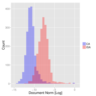
Figure 2: Distribution of $\log\left\lVert U_{i\cdot}\right\rVert_{2}^{2}$ for correspondence analysis with and without ISA. Using ISA increases the influence of the median document in learning topics.

Finally, we note that there exist several topic models that do not reduce to an SVD (e.g., Blei et al., 2003; Hofmann, 2001; Xu et al., 2003); in fact, one of the motivations for latent Dirichlet allocation (Blei et al., 2003) was to add regularization to topic modeling using a hierarchical Bayesian approach. Moreover, methods that only rely on unsupervised topic learning do not in general achieve state-of-the-art accuracy for sentiment classification on their own (e.g., Wang and Manning, 2012). Thus, our goal here is not to advocate an end-to-end methodology for sentiment classification, but only to show that stable autoencoding can substantially improve the quality of topics learned by a simple SVD in cases where a practitioner may want to use them.

6.2 A sensory analysis of perfumes

Finally, we use stable autoencoding to regularize a sensory analysis of perfumes. The data for the analysis was collected by asking consumers to describe 12 luxury perfumes such as Chanel Number 5 and J’adore with words. The answers were then organized in a $12\times 39$ (39 words unique were used) data matrix where each cell represents the number of times a word is associated to a perfume; a total of $N=1075$ were used overall. The dataset is available at http://factominer.free.fr/docs/perfume.txt. We used correspondence analysis (CA) to visualize the associations between words and perfumes. Here, the technique allows to highlight perfumes that were described using a similar profile of words, and to find words that describe the differences between groups of perfumes.

In order to get a better idea of which regularization method is the most trustworthy here, we ran a small bootstrap simulation study built on top of the perfume dataset. We used the full $N=1075$ perfume dataset as the population dataset, and then generated samples of size $N=200$ by subsampling the original dataset without replacement. Then, on each sample, we performed a classical correspondence analysis by performing a rank-$k$ truncated SVD of the matrix $M$ (24), as well as several regularized alternatives described in Section 5.1.

For each estimator, we report its singular values, as well as the RV-coefficients between its row (respectively column) coordinates and the population ones. All the methods except for ISA require us to specify the rank $k$ as an input parameter. Here, of course, $k$ is unknown since we are working with a real dataset; however, examining the full-population dataset suggests that using $k=2$ components is appropriate. For LN, SA and ISA, we set tuning parameters as in Section 5.2, namely LN uses $\hat{\sigma}$ from (31), while SA is performed with $\delta=0.5$. For ISA we used $\delta=0.3$; this latter choice was made to get rank-2 estimates. In practice, one could also consider cross-validation to find a good value for $\delta$.

	$d_{1}$	$d_{2}$	RV row	RV col	$k$
TRUE	0.44	0.15
CA	0.62	0.42	0.41	0.72
LN	0.28	0.11	0.47	0.79
SA	0.34	0.18	0.50	0.79
ISA	0.40	0.18	0.52	0.81	2.43

Table 6: Performance of standard correspondence analysis (CA) as well as regularized alternatives on the perfume dataset. We report singular values, RV-coefficients and rank estimates; results correspond to the mean over the 1000 simulations.

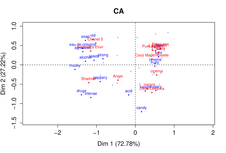
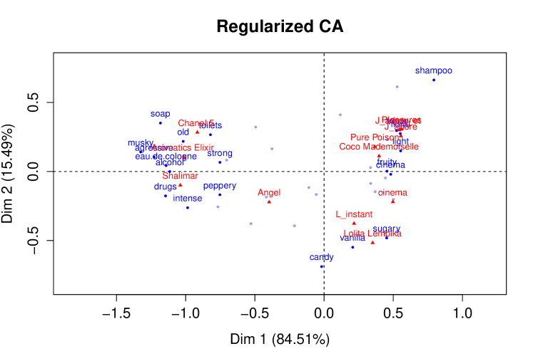
Figure 3: Results for CA on a sample data set (top) and Regularized CA (bottom) using ISA on a single subsample of size $N=200$. Only the 20 words that contribute the most to the dimensions of variability are represented.

Results are shown in Table 6. From a practical point of view, it is also interesting to compare the graphical output of correspondence analysis with and without regularization. Figure 3 (top) shows two-dimensional CA representation on one sample and Figure 3 (bottom) shows the representation obtained with ISA. Only the 20 words that contribute the most to the first two dimensions are represented. The analysis is performed using the R package FactoMineR (Lê et al., 2008).

Our results emphasize that, although correspondence analysis is often used as a visualization technique, appropriate regularization is still important, as regularization may substantially affect the graphical output. For example, on the basis of the CA plot, the perfume Shalimar looks like an outlier, whereas after regularization it seems to fit in a cluster with Chanel 5 and Elixir. We know from Table 6 that the regularized CA plots are better aligned with the population ones than the unregularized ones are; thus, we may be more inclined to trust insights from the regularized analysis.

7 Discussion

In this paper, we introduced a new framework for low-rank matrix estimation that works by transforming noise models into regularizers via a bootstrap scheme. Our method can adapt to non-isotropic noise structures, thus enabling it to substantially outperform its competitors on problems with, e.g., Poisson noise.

At a high level, our framework works by creating pseudo-datasets $\widetilde{X}$ from $X$ using the bootstrap distribution $\widetilde{\mathcal{L}}\left(X\right)$. If two pseudo-datasets $\widetilde{X}_{1}$ and $\widetilde{X}_{2}$ are both likely given $\widetilde{\mathcal{L}}\left(X\right)$, then we want the induced mean estimates $\tilde{\mu}^{1}_{k}=\widetilde{X}_{1}\widehat{B}_{k}$ and $\tilde{\mu}^{2}_{k}=\widetilde{X}_{2}\widehat{B}_{k}$ to be close to each other. The stable autoencoder (6) enables us to turn this intuition into a concrete regularizer by using the Lévy bootstrap. It remains to be seen whether this idea of regularization via bootstrapping pseudo-datasets can be extended to other classes of low-rank matrix algorithms, e.g., those discussed by Collins et al. (2001), de Leeuw (2006), or Udell et al. (2014).

8 Appendix: Proofs

8.1 Proof of Theorem 1

We begin by establishing the equivalence between (6) and (15). By bias-variance decomposition, we can check that

$$\mathbb{E}_{\varepsilon_{ij}\,{\buildrel\text{iid}\over{\sim}\,}\mathcal{N}\left(0,\,\sigma^{2}\right)}\left[\left\lVert X-\left(X+\varepsilon\right)B\right\rVert_{2}^{2}\right] =\left\lVert X-XB\right\rVert_{2}^{2}+\mathbb{E}_{\varepsilon}\left[\left\lVert\varepsilon B\right\rVert^{2}_{2}\right]$$

$$=\left\lVert X-XB\right\rVert_{2}^{2}+\sum_{i,j,k}\operatorname{Var}\left[\varepsilon_{ij}\right]B_{jk}^{2}$$

$$=\left\lVert X-XB\right\rVert_{2}^{2}+n\,\frac{\delta\,\sigma^{2}}{1-\delta}\left\lVert B\right\rVert_{2}^{2},$$

and so the two objectives are equivalent.

To show that $\hat{\mu}_{k}^{\operatorname{stable}}$ can be written as (16), we solve for $\hat{\mu}^{\operatorname{stable}}_{k}=X\widehat{B}_{k}$ explicitly, where

$$\widehat{B}_{k}=\operatorname{argmin}_{B}\left\{\left\lVert X-XB\right\rVert_{2}^{2}+\lambda\left\lVert B\right\rVert_{2}^{2}:\operatorname{rank}\left(B\right)\leq k\right\}.$$

Let $X=UDV^{\top}$ be the SVD of $X$. For any matrix $M$ of the same dimension as $D$, $||UMV^{\top}||_{2}^{2}=||M||_{2}^{2}$. Thus, we can equivalently write the problem

$$\widehat{B}_{k}=V\widehat{Q}_{k}V^{\top},\text{ where }\widehat{Q}_{k}=\operatorname{argmin}_{Q}\left\{\left\lVert D-DQ\right\rVert_{2}^{2}+\lambda\left\lVert Q\right\rVert_{2}^{2}:\operatorname{rank}\left(Q\right)\leq k\right\}.$$

Now, because $D$ is diagonal, $(DQ)_{ij}=D_{ii}Q_{ij}$. Thus, we conclude that $\widehat{Q}_{ij}=0$ for all $i\neq j$, while the problem separates for all the diagonal terms. Without the rank constraint on $Q$, we find that the diagonal terms $\widehat{Q}_{ii}$ are given by

$$\widehat{Q}_{ii}=\operatorname{argmin}_{Q_{ii}}\left\{\left(1-Q_{ii}\right)^{2}D_{ii}^{2}+\lambda\,Q_{ii}^{2}\right\}=\frac{D_{ii}^{2}}{\lambda+D_{ii}^{2}}.$$

Meanwhile, we can check that adding the rank constraint amounts to zeroing out all but the $k$ largest of the $\widehat{Q}_{ii}$. Thus, plugging this into our expression of $\hat{\mu}$, we get that

$$\hat{\mu}_{k}^{\operatorname{stable}}=\sum_{i=1}^{k}U_{i.}\frac{D_{ii}}{1+\lambda/D_{ii}^{2}}V_{i.}^{\top}.$$

8.2 Proof of Theorem 2

We start by showing that $\widehat{B}$ is the solution to the unconstrained version of (17). Let $V$ be a matrix defined by

$$V_{ij}=\operatorname{Var}_{\widetilde{X}\sim\widetilde{\mathcal{L}}\left(X\right)}\left[\widetilde{X}_{ij}\right].$$

Because $\widetilde{X}$ has mean $X$, we can check that

$$\mathbb{E}_{\widetilde{X}\sim\widetilde{\mathcal{L}}\left(X\right)}\left[\left\lVert X-\widetilde{X}B\right\rVert_{2}^{2}\right]=\left\lVert X-XB\right\rVert_{2}^{2}+\sum_{i,j,k}V_{ij}\,B^{2}_{jk}.$$

Thus,

$$\frac{1}{2}\,\frac{\partial}{\partial B_{jk}}\mathbb{E}_{\widetilde{X}\sim\widetilde{\mathcal{L}}\left(X\right)}\left[\left\lVert X-\widetilde{X}B\right\rVert_{2}^{2}\right]=-\sum_{i}X_{ij}\left(X-XB\right)_{ik}+\sum_{i}V_{ij}\,B_{jk}.$$

Setting gradients to zero, we find an equilibrium

$$X^{\top}X=X^{\top}XB+SB,\;\text{ where }S_{jk}=\begin{cases}\sum_{i=1}^{n}V_{ij}&\text{for }j=k,\\ 0&\text{else.}\end{cases}$$

Thus, we conclude that

$$\widehat{B}=\left(X^{\top}X+S\right)^{-1}\,X^{\top}X$$

is in fact the solution to (17) without the rank constraint.

Next, we show how we can get from $\widehat{B}$ to $\widehat{B}_{k}$ using (19). For any matrix $B$, we can verify by quadratic expansion that

$$\left\lVert X-XB\right\rVert_{2}^{2} =\left\lVert X-X\widehat{B}\right\rVert_{2}^{2}+\left\lVert X\left(\widehat{B}-B\right)\right\rVert_{2}^{2}+2\operatorname{tr}\left(\left(X-X\widehat{B}\right)^{\top}\left(X\widehat{B}-XB\right)\right)$$

$$=\left\lVert X-X\widehat{B}\right\rVert_{2}^{2}+\left\lVert X\left(\widehat{B}-B\right)\right\rVert_{2}^{2}$$

$$\ \ \ \ \ \ +2\operatorname{tr}\left(\left(X^{\top}X\left(X^{\top}X+S\right)^{-1}X^{\top}X-X^{\top}X\right)\left(B-\widehat{B}\right)\right)$$

Meanwhile,

$$\left\lVert S^{\frac{1}{2}}B\right\rVert^{2} =\left\lVert S^{\frac{1}{2}}\widehat{B}\right\rVert_{2}^{2}+\left\lVert S^{\frac{1}{2}}\left(B-\widehat{B}\right)\right\rVert_{2}^{2}+2\operatorname{tr}\left(\widehat{B}^{\top}S\left(B-\widehat{B}\right)\right)$$

$$=\left\lVert S^{\frac{1}{2}}\widehat{B}\right\rVert_{2}^{2}+\left\lVert S^{\frac{1}{2}}\left(B-\widehat{B}\right)\right\rVert_{2}^{2}+2\operatorname{tr}\left(X^{\top}X\left(X^{\top}X+S\right)^{-1}S\left(B-\widehat{B}\right)\right).$$

Summing everything together, we find that

$$\left\lVert X-XB\right\rVert_{2}^{2}+\left\lVert S^{\frac{1}{2}}B\right\rVert^{2}=\left\lVert X\left(B-\widehat{B}\right)\right\rVert_{2}^{2}+\left\lVert S^{\frac{1}{2}}\left(B-\widehat{B}\right)\right\rVert_{2}^{2}+R\left(\widehat{B},\,X\right)$$

where $R$ is a residual term that does not depend on $B$. Thus, we conclude that

$$\widehat{B}_{k} =\operatorname{argmin}_{B}\left\{\left\lVert X-XB\right\rVert_{2}^{2}+\left\lVert S^{\frac{1}{2}}B\right\rVert_{2}^{2}:\operatorname{rank}\left(B\right)\leq k\right\}$$

$$=\operatorname{argmin}_{B}\left\{\operatorname{tr}\left(\left(B-\widehat{B}\right)^{\top}\left(X^{\top}X+S\right)\left(B-\widehat{B}\right)\right):\operatorname{rank}\left(B\right)\leq k\right\}.$$

As shown in, e.g., Takane (2013), we can solve this last problem by taking the top $k$ terms of the eigendecomposition of $\widehat{B}^{\top}\left(X^{\top}X+S\right)^{-1}\widehat{B}$.

8.3 Proof of Theorem 3

For iterates $t=0,\,1,\,...$, define $M_{t}=\hat{\mu}_{t}^{\top}\hat{\mu}_{t}$. Here, we will show that $M_{t}$ converges to a fixed point $M^{*}$, and that $M^{*}\preceq X^{\top}X$; the desired conclusion then follows immediately. First, by construction, we have that

$$M_{0}=X^{\top}X\;\text{ and }\;M_{1}=X^{\top}X\left(X^{\top}X+S\right)^{-1}X^{\top}X\left(X^{\top}X+S\right)^{-1}X^{\top}X,$$

and so we immediately see that $M_{1}\preceq M_{0}$. The general update for $M_{t}$ is

$$M_{t+1}=g\left(M_{t}\right)^{\top}g\left(M_{t}\right),\;\text{ where }g\left(M\right)=\Sigma^{\frac{1}{2}}\left(M+S\right)^{-1}M,$$ (33)

where $\Sigma^{\frac{1}{2}}$ is a positive semi-definite solution to $(\Sigma^{\frac{1}{2}})^{\top}\Sigma^{\frac{1}{2}}=X^{\top}X$. Now, because matrix inversion is a monotone decreasing function over the positive semi-definite cone and $S\succ 0$, we find that

$$g(M)=\Sigma^{\frac{1}{2}}\left(I-\left(M+S\right)^{-1}S\right)$$

is monotone increasing in $M$ over the positive semi-definite cone. In particular

$$\text{if}\;M_{t}\preceq M_{t-1},\;\text{then}\;M_{t+1}\preceq M_{t}.$$

By induction, the sequence $M_{t}$ is monotone decreasing with respect to the positive semi-definite cone order; by standard arguments, it thus follows that this sequence must converge to a limit $M^{*}$. Finally, we note that convergence of $M_{t}$ also implies convergence of $\hat{\mu}_{t}$, since $\hat{\mu}_{t+1}=X\widehat{B}_{t}$ and $\widehat{B}_{t}$ only depends on $\hat{\mu}_{t}$ through $M_{t}$.

8.4 Proof of Theorem 4

As in the proof of Theorem 3, let $M^{*}=\hat{\mu}^{\top}\hat{\mu}$. Because $M^{*}$ is a fixed point, we know that

$$M^{*}=M^{*}\left(M^{*}+S\right)^{-1}X^{\top}X\left(M^{*}+S\right)^{-1}M^{*}.$$

Now, because $M^{*}$ is symmetric with eigenvector $u$, we can decompose it as

$$M^{*}=M^{\perp}+\lambda_{u}uu^{\top},\;\text{ where }\;\lambda_{u}=u^{\top}M^{*}u\;\text{ and }\;\left\lVert M^{\perp}u\right\rVert_{2}=0.$$

By combining these equalities and using the monotonicity of matrix inversion, we find that

$$\lambda_{u} =u^{\top}M^{*}u$$

$$=\lambda_{u}^{2}\,u^{\top}\left(M^{*}+S\right)^{-1}X^{\top}X\left(M^{*}+S\right)^{-1}u$$

$$\leq\lambda_{u}^{2}\,u^{\top}S^{-1}X^{\top}XS^{-1}u.$$

This relation can only hold if $\lambda_{u}=0$, or $1\leq\lambda_{u}\,u^{\top}S^{-1}X^{\top}XS^{-1}u$, and so our desired conclusion must hold.

8.5 Proof of Proposition 5

First, we note that in the setting (14) with $\delta=1/2$, we have $S=n\sigma^{2}I$. Using Theorem 1, we can verify that the singular vectors of $\hat{\mu}_{t}$ are the same as those of $X$ for each iterate $t=1,\,2,\,...$ of our algorithm; and so we can write the limit $\hat{\mu}^{{\operatorname{iter}}}$ as singular value shrinker

$$\hat{\mu}^{{\operatorname{iter}}}=\sum_{l=1}^{\min\{n,\,p\}}u_{l}\,\psi\left(d_{l}\right)\,v_{l}^{\top}.$$

It remains to derive the form of $\psi$. Now, using (16), we can verify that the fixed point condition on $\hat{\mu}^{{\operatorname{iter}}}$ can be expressed in terms of $\psi$ as

$$\psi(d)=\frac{\psi^{2}(d)}{\lambda+\psi^{2}(d)}\,d,\ \text{ with }\ \lambda=n\sigma^{2}.$$

This is a cubic equation, with solutions

$$\psi(d)=0,\ \text{ and }\ \psi(d)=\frac{1}{2}\left(d\pm\sqrt{d^{2}-4n\sigma^{2}}\right)\ \text{ for }\ d^{2}\geq 4n\sigma^{2}.$$

Finally, we can verify that our iterative procedure cannot jump over the largest root, thus resulting in the claimed shrinkage function.

We also check here that, in the case $n=p$, our shrinker $\psi(\cdot)$ is equivalent to the asymptotically optimal shrinker for operator loss $\psi^{*}_{op}(d)$ (Gavish and Donoho, 2014b) which is 0 for $d^{2}<4n\sigma^{2}$, and else

$$\psi_{op}(d) =\frac{1}{\sqrt{2}}\,\sqrt{d^{2}-2n\sigma^{2}+\sqrt{\left(d^{2}-2n\sigma^{2}\right)^{2}-4n^{2}\sigma^{4}}}$$

$$=\frac{1}{\sqrt{2}}\,\sqrt{d^{2}-2n\sigma^{2}+d\,\sqrt{d^{2}-4n\sigma^{2}}}.$$

Squaring our iterative shrinker, we see that

$$\psi^{2}(d)=\frac{1}{2}\left(d^{2}-2n\sigma^{2}+d\sqrt{d^{2}-4n\sigma^{2}}\right)=\psi^{2}_{op}(d)$$

for $d^{2}\geq 4n\sigma^{2}$, and 0 else.

References

- Baldi and Hornik (1989) Pierre Baldi and Kurt Hornik. Neural networks and principal component analysis: Learning from examples without local minima. Neural Networks, 2(1):53–58, 1989.
- Baldi and Sadowski (2014) Pierre Baldi and Peter Sadowski. The dropout learning algorithm. Artificial Intelligence, 210:78–122, 2014.
- Benzécri (1973) J-P Benzécri. L’analyse des données. Tome II: L’analyse des correspondances. Dunod, 1973.
- Benzécri (1986) J.-P. Benzécri. Statistical analysis as a tool to emerge patterns from the data. In S. Watanabe (ed), editor, Methodologies of Pattern recognition, pages 34–74. New-York, Academic Press, 1986.
- Bishop (1995) Chris M Bishop. Training with noise is equivalent to Tikhonov regularization. Neural Computation, 7(1):108–116, 1995.
- Blei et al. (2003) David M Blei, Andrew Y Ng, and Michael I Jordan. Latent Dirichlet allocation. The Journal of Machine Learning Research, 3:993–1022, 2003.
- Bourlard and Kamp (1988) Hervé Bourlard and Yves Kamp. Auto-association by multilayer perceptrons and singular value decomposition. Biological Cybernetics, 59(4-5):291–294, 1988.
- Breiman (1996) Leo Breiman. Bagging predictors. Machine learning, 24(2):123–140, 1996.
- Buja and Stuetzle (2006) Andreas Buja and Werner Stuetzle. Observations on bagging. Statistica Sinica, pages 323–351, 2006.
- Buntine (2002) Wray Buntine. Variational extensions to EM and multinomial PCA. In Tapio Elomaa, Heikki Mannila, and Hannu Toivonen, editors, Machine Learning: ECML 2002, Lecture Notes in Computer Science, pages 23–34. Springer Berlin Heidelberg, 2002.
- Cai et al. (2010) Jian-Feng Cai, Emmanuel J Candès, and Zuowei Shen. A singular value thresholding algorithm for matrix completion. SIAM Journal on Optimization, 20(4):1956–1982, 2010.
- Candès and Tao (2010) Emmanuel J Candès and Terence Tao. The power of convex relaxation: Near-optimal matrix completion. IEEE Transactions on Information Theory, 56(5):2053–2080, 2010.
- Candès et al. (2013) Emmanuel J Candès, Carlos A Sing-Long, and Joshua D Trzasko. Unbiased risk estimates for singular value thresholding and spectral estimators. IEEE Transactions on Signal Processing, 61(19):4643–4657, 2013.
- Chatterjee (2015) Sourav Chatterjee. Matrix estimation by universal singular value thresholding. The Annals of Statistics, 43(1):177–214, 2015.
- Collins et al. (2001) Michael Collins, Sanjoy Dasgupta, and Robert E. Schapire. A generalization of principal component analysis to the exponential family. In Advances in Neural Information Processing Systems. MIT Press, 2001.
- d’Aspremont et al. (2012) Alexandre d’Aspremont, Francis Bach, and Laurent El Ghaoui. Approximation bounds for sparse principal component analysis. Mathematical Programming, pages 1–22, 2012.
- de Leeuw (2006) Jan de Leeuw. Principal component analysis of binary data by iterated singular value decomposition. Computational Statistics and Data Analysis, 50(1):21–39, 2006.
- Deerwester et al. (1990) Scott C. Deerwester, Susan T Dumais, Thomas K. Landauer, George W. Furnas, and Richard A. Harshman. Indexing by latent semantic analysis. Journal of the American Society for Information Science, 41(6):391–407, 1990.
- Durrett (2010) Rick Durrett. Probability: Theory and Examples. Cambridge University Press, 2010.
- Efron (2012) Bradley Efron. Large-Scale Inference: Empirical Bayes Methods for Estimation, Testing, and Prediction. Cambridge University Press, 2012.
- Efron and Tibshirani (1993) Bradley Efron and Robert Tibshirani. An Introduction to the Bootstrap. Chapman & Hall/CRC, 1993.
- Escoufier (1973) Yves Escoufier. Le traitement des variables vectorielles. Biometrics, 29:751–760, 1973.
- Fithian and Mazumder (2013) William Fithian and Rahul Mazumder. Scalable convex methods for flexible low-rank matrix modeling. arXiv preprint arXiv:1308.4211, 2013.
- Gavish and Donoho (2014a) Matan Gavish and David L Donoho. The optimal hard threshold for singular values is 4/sqrt (3). IEEE Transactions on Information Theory, 60(8), 2014a.
- Gavish and Donoho (2014b) Matan Gavish and David L Donoho. Optimal shrinkage of singular values. arXiv:1405.7511v2, 2014b.
- Globerson and Roweis (2006) Amir Globerson and Sam Roweis. Nightmare at test time: Robust learning by feature deletion. In Proceedings of the International Conference on Machine Learning, 2006.
- Goodfellow et al. (2013) Ian Goodfellow, David Warde-farley, Mehdi Mirza, Aaron Courville, and Yoshua Bengio. Maxout networks. In Proceedings of the 30th International Conference on Machine Learning, pages 1319–1327, 2013.
- Goodman (1985) L. A. Goodman. The analysis of cross-classified data having ordered and/or unordered categories: Association models, correlation models, and asymmetry models for contingency tables with or without missing entries. Annals of Statistics, 13:10–69, 1985.
- Greenacre (1984) Michael J Greenacre. Theory and Applications of Correspondence Analysis. Acadamic Press, 1984.
- Greenacre (2007) Michael J Greenacre. Correspondence Analysis in Practice, Second Edition. Chapman & Hall, 2007.
- Hirschfeld (1935) Hermann O Hirschfeld. A connection between correlation and contingency. Mathematical Proceedings of the Cambridge Philosophical Society, 31(4):520–524, 1935.
- Hofmann (2001) Thomas Hofmann. Unsupervised learning by probabilistic latent semantic analysis. Machine Learning, 42(1-2):177–196, 2001.
- Johnstone (2001) Ian Johnstone. On the distribution of the largest eigenvalue in principal components analysis. The Annals of Statistics, 29(2):295–327, 2001.
- Jolliffe (2002) Ian Jolliffe. Principal Component Analysis. Springer, 2002.
- Jolliffe et al. (2003) Ian T Jolliffe, Nickolay T Trendafilov, and Mudassir Uddin. A modified principal component technique based on the lasso. Journal of Computational and Graphical Statistics, 12(3):531–547, 2003.
- Josse and Holmes (2013) Julie Josse and Susan Holmes. Measures of dependence between random vectors and tests of independence. Literature review. arXiv preprint arXiv:1307.7383, 2013.
- Josse and Husson (2011) Julie Josse and François Husson. Selecting the number of components in PCA using cross-validation approximations. Computational Statististics and Data Analysis, 56(6):1869–1879, 2011.
- Josse and Sardy (2015) Julie Josse and Sylvain Sardy. Adaptive shrinkage of singular values. Statistics and Computing, pages 1–10, 2015.
- Josse et al. (2016) Julie Josse, Sylvain Sardy, and Stefan Wager. denoiseR: A package for low rank matrix estimation. arXiv preprint arXiv:1602.01206, 2016.
- Koren et al. (2009) Yehuda Koren, Robert Bell, and Chris Volinsky. Matrix factorization techniques for recommender systems. Computer, 42(8):30–37, 2009.
- Krizhevsky et al. (2012) Alex Krizhevsky, Ilya Sutskever, and Geoffrey E Hinton. Imagenet classification with deep convolutional neural networks. In Advances in Neural Information Processing Systems, pages 1097–1105, 2012.
- Kucukelbir and Blei (2015) Alp Kucukelbir and David M Blei. Population empirical Bayes. Uncertainty in Artificial Intelligence, 2015.
- Lê et al. (2008) Sébastien Lê, Julie Josse, and François Husson. FactoMineR: An R package for multivariate analysis. Journal of Statistical Software, 25(1):1–18, 2008.
- Leek and Storey (2007) Jeffrey T Leek and John D Storey. Capturing heterogeneity in gene expression studies by surrogate variable analysis. PLoS genetics, 3(9):e161, 2007.
- Li and Tao (2013) J. Li and D. Tao. Simple exponential family PCA. IEEE Transactions on Neural Networks and Learning Systems, 24(3):485–497, 2013.
- Lustig et al. (2008) Michael Lustig, David L Donoho, Juan M Santos, and John M Pauly. Compressed sensing MRI. Signal Processing Magazine, IEEE, 25(2):72–82, 2008.
- Ng et al. (2002) Andrew Y Ng, Michael I Jordan, and Yair Weiss. On spectral clustering: Analysis and an algorithm. Advances in Neural Information Processing Systems, 2:849–856, 2002.
- Owen and Eckles (2012) Art B Owen and Dean Eckles. Bootstrapping data arrays of arbitrary order. The Annals of Applied Statistics, 6(3):895–927, 2012.
- Pang and Lee (2004) Bo Pang and Lillian Lee. A sentimental education: Sentiment analysis using subjectivity summarization based on minimum cuts. In Proceedings of the Association for Computational Linguistics, page 271. Association for Computational Linguistics, 2004.
- Price et al. (2006) Alkes L Price, Nick J Patterson, Robert M Plenge, Michael E Weinblatt, Nancy A Shadick, and David Reich. Principal components analysis corrects for stratification in genome-wide association studies. Nature Genetics, 38(8):904–909, 2006.
- Robbins (1985) Herbert Robbins. The Empirical Bayes Approach to Statistical Decision Problems. Springer, 1985.
- Shabalin and Nobel (2013) Andrey A Shabalin and Andrew B Nobel. Reconstruction of a low-rank matrix in the presence of Gaussian noise. Journal of Multivariate Analysis, 118:67–76, 2013.
- Shi and Malik (2000) Jianbo Shi and Jitendra Malik. Normalized cuts and image segmentation. Pattern Analysis and Machine Intelligence, IEEE Transactions on, 22(8):888–905, 2000.
- Simard et al. (2000) Patrice Y Simard, Yann A Le Cun, John S Denker, and Bernard Victorri. Transformation invariance in pattern recognition: Tangent distance and propagation. International Journal of Imaging Systems and Technology, 11(3):181–197, 2000.
- Srivastava et al. (2014) Nitish Srivastava, Geoffrey Hinton, Alex Krizhevsky, Ilya Sutskever, and Ruslan Salakhutdinov. Dropout: A simple way to prevent neural networks from overfitting. The Journal of Machine Learning Research, 15(1):1929–1958, 2014.
- Takane (2013) Yoshio Takane. Constrained Principal Component Analysis and Related Techniques. Chapman & Hall, 2013.
- Tibshirani (1996) Robert Tibshirani. Regression shrinkage and selection via the lasso. Journal of the Royal Statistical Society. Series B (Methodological), pages 267–288, 1996.
- Udell et al. (2014) Madeleine Udell, Corinne Horn, Reza Zadeh, and Stephen Boyd. Generalized low rank models. arXiv preprint arXiv:1410.0342, 2014.
- van der Maaten et al. (2013) Laurens van der Maaten, Minmin Chen, Stephen Tyree, and Kilian Q Weinberger. Learning with marginalized corrupted features. In Proceedings of the International Conference on Machine Learning, 2013.
- Verbanck et al. (2013) Marie Verbanck, Julie Josse, and François Husson. Regularised PCA to denoise and visualise data. Statistics and Computing, pages 1–16, 2013.
- Wager et al. (2013) Stefan Wager, Sida Wang, and Percy Liang. Dropout training as adaptive regularization. In Advances in Neural Information Processing Systems, pages 351–359, 2013.
- Wager et al. (2014) Stefan Wager, William Fithian, Sida Wang, and Percy Liang. Altitude training: Strong bounds for single-layer dropout. In Advances in Neural Information Processing Systems, volume 27, pages 100–108, 2014.
- Wager et al. (2016) Stefan Wager, William Fithian, and Percy Liang. Data augmentation via Lévy processes. arXiv preprint arXiv:1603.06340, 2016.
- Wang and Manning (2012) Sida Wang and Christopher D Manning. Baselines and bigrams: Simple, good sentiment and topic classification. In Proceedings of the Association for Computational Linguistics, pages 90–94. Association for Computational Linguistics, 2012.
- Wang et al. (2013) Sida I Wang, Mengqiu Wang, Stefan Wager, Percy Liang, and Christopher D Manning. Feature noising for log-linear structured prediction. In Empirical Methods in Natural Language Processing, 2013.
- Witten et al. (2009) Daniela M Witten, Robert Tibshirani, and Trevor Hastie. A penalized matrix decomposition, with applications to sparse principal components and canonical correlation analysis. Biostatistics, 2009.
- Xu et al. (2003) Wei Xu, Xin Liu, and Yihong Gong. Document clustering based on non-negative matrix factorization. In ACM SIGIR Conference on Research and Development in Information Retrieval, pages 267–273. ACM, 2003.
- Zhang and Huang (2008) C. H. Zhang and J. Huang. The sparsity and bias of the lasso selection in high-dimensional linear regression. The Annals of Statistics, 36(4):1567–1594, 2008.
- Zou (2006) H. Zou. The adaptive LASSO and its oracle properties. Journal of the American Statistical Association, 101:1418–1429, 2006.
- Zou et al. (2006) H. Zou, T. Hastie, and R. Tibshirani. Sparse principal component analysis. Journal of Computational and Graphical Statistics, 15(2):265–286, 2006.