Stochastic Komatu-Loewner evolutions
and BMD domain constant

Abstract

Let $D={\mathbb{H}}\setminus\cup_{k=1}^{N}C_{k}$ be a standard slit domain, where $\mathbb{H}$ is the upper half plane and $C_{k}$, $1\leq k\leq N$, are mutually disjoint horizontal line segments in ${\mathbb{H}}$. Given a Jordan arc $\gamma\subset D$ starting at $\partial{\mathbb{H}},$ let $g_{t}$ be the unique conformal map from $D\setminus\gamma[0,t]$ onto a standard slit domain $D_{t}={\mathbb{H}}\setminus\cup_{k=1}^{N}C_{k}(t)$ satisfying the hydrodynamic normalization at infinity. It has been established recently that $g_{t}$ satisfies an ODE called a Komatu-Loewner equation in terms of the complex Poisson kernel of the Brownian motion with darning (BMD) for $D_{t}$, extending the classical chordal Loewner equation for the simply connected domain $D={\mathbb{H}}.$

We randomize the Jordan arc $\gamma$ according to a system of probability measures on the family of equivalence classes of Jordan arcs that enjoy a domain Markov property and a certain conformal invariance property. We show that the induced process $(\xi(t),{\bf s}(t))$ satisfies a Markov type stochastic differential equation, where $\xi(t)$ is a motion on $\partial{\mathbb{H}}$ and ${\bf s}(t)$ represents the motion of the endpoints of the slits $\{C_{k}(t),\;1\leq k\leq N\}.$ The diffusion and drift coefficients $\alpha$ and $b$ of $\xi(t)$ are homogeneous functions of degree $0$ and $-1$, respectively, while ${\bf s}(t)$ has drift coefficients only, determined by the BMD complex Poisson kernel that are known to be Lipschitz continuous.

Conversely, given such functions $\alpha$ and $b$ with local Lipschitz continuity, the corresponding SDE admits a unique solution $(\xi(t),{\bf s}(t))$. The latter produces random conformal maps $g_{t}(z)$ via the Komatu-Loewner equation. The resulting family of random growing hulls $\{F_{t}\}$ from the conformal mappings is called ${\rm SKLE}_{\alpha,b}.$ We show that it enjoys a certain scaling property and a domain Markov property. Among other things, we further prove that ${\rm SKLE}_{\alpha,-b_{\rm BMD}}$ for a constant $\alpha>0$ has a locality property if and only if $\alpha=\sqrt{6}$, where $b_{\rm BMD}$ is a BMD-domain constant that describes the discrepancy of a standard slit domain from ${\mathbb{H}}$ relative to BMD.

AMS 2010 Mathematics Subject Classification: Primary 60J67, 60J70; Secondary 30C20, 60H10, 60H30

Keywords and phrases: Stochastic Komatu-Loewner evolution, Brownian motion with darning, Komatu-Loewner equation for slits, SDE with homogeneous coefficients, generalized Komatu-Loewner equation for image hulls, BMD domain constant, locality property

1 Introduction

In 2000, Oded Schramm [S] introduced a stochastic Loewner evolution (SLE) on the upper half plane ${\mathbb{H}}$ with driving process $\xi(t)=\sqrt{\kappa}B_{t}$, where $B_{t}$ is the standard Brownian motion on $\partial{\mathbb{H}}$ and $\kappa$ is a positive constant. The solution of the SLE is a family of random conformal mappings from ${\mathbb{H}}\setminus K_{t}$ to ${\mathbb{H}}$ indexed by $t\geq 0$. The increasing family of random hulls $\{K_{t};t\geq 0\}$ is nowadays called ${\rm SLE}_{\kappa}$. It has a certain conformal invariance and a domain Markov property. ${\rm SLE}_{\kappa}$ is a powerful tool in studying two-dimensional critical systems in statistical physics. ${\rm SLE}_{\kappa}$ has been proved to be the scaling limit of various critical two-dimensional lattice models, such as loops erased random walk, uniform spanning trees, critical percolation, critical Ising model, and has been conjectured for a few more including self-avoiding random walks. In particular, ${\rm SLE}_{6}$ was found to have a special property called locality by Lawler-Schramm-Werner [LSW1, LSW2]. Later, it was proved by S. Smirnov that ${\rm SLE}_{6}$ is the scaling limit of the critical percolation exploration process on two-dimensional triangular lattice. In honor of Schramm, SLE is now also called Schramm-Loewner evolution.

In this paper, we extend the SLE theory from the upper half plane ${\mathbb{H}}$ to a standard slit domain –a specific canonical multiply connected planar domain. Based on recent results of Chen-Fukushima-Rhode [CFR] on chordal Komatu-Loewner (KL) equation and following the lines briefly laid by R. O. Bauer and R. M. Friedrich [BF1, BF2, BF3], we show that, for a corresponding evolution in a standard slit domain $D={\mathbb{H}}\setminus\bigcup_{k=1}^{N}C_{k}$, the possible candidates of the driving processes are given by the solution $(\xi(t),{\bf s}(t))$ of a special Markov type stochastic differential equation whose diffusion and drift coefficients are homogeneous function of degree $0$ and $-1$, respectively. Here $\xi(t)$ is a motion on $\partial{\mathbb{H}}$ and ${\bf s}(t)$ is a motion of slits $C_{k},\;1\leq k\leq N$. When no slit is present, $\xi(t)$ becomes $\sqrt{\kappa}B_{t}$ as in the simply connected domain ${\mathbb{H}}$ case. The solution $(\xi(t),{\bf s}(t))$ of the SDE then produces a family of random conformal mappings from the multiply connected domains $D\setminus F_{t}$ to the canonical slit domains $D({\bf s}(t))$ via KL equations. This family or its associated increasing family of random growing ${\mathbb{H}}$-hulls $\{F_{t};t\geq 0\}$ is called a stochastic Komatu-Loewner evolution (SKLE in abbreviation). We then study the locality property of SKLE.

We now recall the setting formulated in [CFR] and some of its results that will be utilized in this paper. They are followed by a detailed description of the rest of the paper.

A domain of the form $D={\mathbb{H}}\setminus\bigcup_{k=1}^{N}C_{k}$ is called a standard slit domain where $\{C_{k}\}$ are mutually disjoint line segments in ${\mathbb{H}}$ parallel to the $x$-axis. Denote by ${\cal D}$ the collection of ’labeled (ordered)’ standard slit domains. For instance, ${\mathbb{H}}\setminus\{C_{1},C_{2},C_{3},\cdots,C_{N}\}$ and ${\mathbb{H}}\setminus\{C_{2},C_{1},C_{3},\cdots,C_{N}\}$ are considered as different elements of ${\cal D}$ in general although they correspond to the same subset ${\mathbb{H}}\setminus\bigcup_{i=1}^{N}C_{i}$ of ${\mathbb{H}}.$ For $D$ and $\widetilde{D}$ in ${\cal D}$, define the distance $d(D,\widetilde{D})$ between them by

$$d(D,\widetilde{D})=\max_{1\leq i\leq N}\left(|z_{k}-\widetilde{z}_{k}|+|z_{k}^{\prime}-\widetilde{z}_{k}^{\prime}|\right),$$ (1.1)

where, $z_{k}$ and $z_{k}^{\prime}$ (respectively, $\widetilde{z}_{k}$ and $\widetilde{z}_{k}^{\prime}$) are the left and right endpoints of the $k$th slit of $D$ (respectively, $\widetilde{D}$).

We fix $D\in{\cal D}$ and consider a Jordan arc

$$\gamma:[0,t_{\gamma})\rightarrow\overline{D}\quad\hbox{with }\ \gamma(0)\in\partial{\mathbb{H}}\ \hbox{ and }\gamma(0,t_{\gamma})\subset D\ \hbox{ for }0<t_{\gamma}\leq\infty.$$ (1.2)

For each $t\in[0,t_{\gamma})$, let

$$g_{t}:D\setminus\gamma[0,t]\rightarrow D_{t}$$ (1.3)

be the unique conformal map from $D\setminus\gamma[0,t]$ onto some $D_{t}={\mathbb{H}}\setminus\bigcup_{k=1}^{N}C_{k}(t)\in{\cal D}$ satisfying a hydrodynamic normalization

$$g_{t}(z)=z+\frac{a_{t}}{z}+o(1/|z|),\qquad z\to\infty.$$ (1.4)

The coefficient $a_{t}$ is called the half-plane capacity of $g_{t}$. The slits $C_{k}(t)$, $1\leq k\leq N$, are uniquely determined by $D$ and $\gamma[0,t]$. See Figure 1.

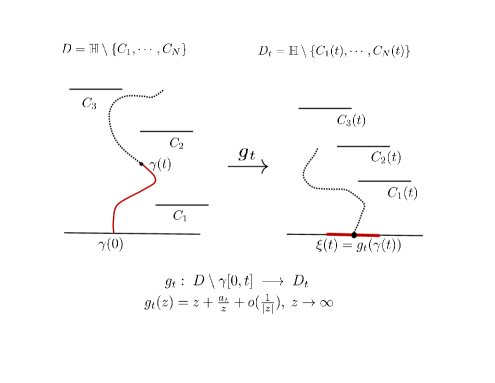
Figure 1: Conformal mapping $g_{t}$

Let ${\bf s}(t)$ denote the endpoints of these slits $C_{k}(t)$ (see (3.1) below for a precise definition) and denote $D_{t}$ by $D({\bf s}(t))$. We also define

$$\xi(t)=g_{t}(\gamma(t))\in\partial{\mathbb{H}},\quad 0\leq t<t_{\gamma}.$$ (1.5)

For a Borel set $A\subset\overline{\mathbb{H}}$, we use $\partial_{p}A$ to denote the boundary of $A$ with respect to the topology induced by the path distance in ${\mathbb{H}}\setminus A$. For instance, when $A\subset{\mathbb{H}}$ is a horizontal line segment, then $\partial_{p}A$ consists of the upper part $A^{+}$ and the lower part $A^{-}$ of the line segment $A$.

In [CFR, Section 8], the following results are established:

(P.1)

For every $0<s<t_{\gamma}$, $g_{t}(z)$ is jointly continuous in $(t,z)\in[0,s]\times((D\cup\partial_{p}K\cup\partial{\mathbb{H}})\setminus\gamma[0,s])$, where $K=\bigcup_{k=1}^{N}C_{k}.$

(P.2)

$a_{t}$ is strictly increasing and continuous in $t\in[0,t_{\gamma})$ with $a_{0}=0$ so that the arc $\gamma$ can be reparametrized in such a way that $a_{t}=2t,\ 0\leq t<t_{\gamma},$ which is called the half-plane capacity parametrization.

(P.3)

$\xi(t)\in\partial{\mathbb{H}}$ is continuous in $t\in[0,t_{\gamma}).$

(P.4)

$D_{t}\in{\cal D}$ is continuous in $t\in[0,t_{\gamma})$ with respect to the metric (1.1) on ${\cal D}$.

Historically $g_{t}(z)$ has been obtained by solving the extremal problem to maximize the coefficient $a_{t}$ among all univalent functions on $D\setminus\gamma[0,t]$ with the hydrodynamic normalization at infinity. But, in order to prove the above continuity properties, we used the following probabilistic representation of $g_{t}(z)$ given in [CFR, §7]:

Let $Z^{{\mathbb{H}},*}=\{Z_{t}^{{\mathbb{H}},*},\ {\mathbb{P}}_{z}^{{\mathbb{H}},*},\ z\in D^{*}\}$ be the Brownian motion with darning (BMD) on $D^{*}:=D\cup\{c_{1}^{*},\dots,c_{N}^{*}\}$ obtained from the absorbing Brownian motion in ${\mathbb{H}}$ by rendering (or shorting) each slit $C_{k}$ into one single point $c_{k}^{*}$. That is, $Z^{{\mathbb{H}},*}$ is an $m$-symmetric diffusion process on $D^{*}$ whose subprocess killed upon leaving $D$ is the absorbing Brownian motion in $D$. Here $m$ is the measure on $D^{*}$ that does not charge on $\{c^{*}_{1},\dots,c_{N}^{*}\}$ and its restriction to $D$ is the Lebesgue measure in $D$. BMD $Z^{{\mathbb{H}},*}$ is unique in law and spends zero Lebesgue amount of time on $\{c^{*}_{1},\dots,c_{N}^{*}\}$; see [CFR] for details. Set $F_{t}:=\gamma[0,t]$, $\Gamma_{r}:=\{z=x+iy:y=r\},\ r>0.$ For a set $A\subset D^{*}$, define $\sigma_{A}=\inf\{t>0:Z_{t}^{{\mathbb{H}},*}\in A\}$. Then (cf. [CFR, Theorem 7.2]

$$\Im\;g_{t}(z)=\lim_{r\to\infty}r\cdot{\mathbb{P}}_{z}^{{\mathbb{H}},*}(\sigma_{\Gamma_{r}}<\sigma_{F_{t}}).$$ (1.6)

Here $\Im g_{t}(z)$ stands for the imaginary part of the conformal map $g_{t}(z)$. The above formula was first obtained by Lawler [L2] with Excursion reflected Brownian motion (ERBM) formulated there in place of BMD. See [CFR, Remark 2.2], [CF2, §6] and Remark 6.13 of the present paper for the relationship between these two processes.

It is proved in [CFR, Theorem 9.9] that the family of conformal maps $\{g_{t}(z);t\geq 0\}$ satisfies the Komatu-Loewner (KL) equation under the half-plane capacity parametrization of $\gamma$:

$$\partial_{t}g_{t}(z)=-2\pi\Psi_{t}(g_{t}(z),\xi(t))\quad\hbox{for }0\leq t<t_{\gamma}\ \hbox{ with }\ g_{0}(z)=z\in(D\cup\partial_{p}K)\setminus\gamma[0,t_{\gamma}),$$ (1.7)

where $\Psi_{t}(z,\xi)$, $z\in D_{t}$, $\xi\in\partial{\mathbb{H}}$, is the BMD-complex Poisson kernel for $D_{t}$, namely, the unique analytic function in $z\in D_{t}$ vanishing at $\infty$ whose imaginary part is the Poisson kernel of the BMD for the standard slit domain $D_{t}$ with pole $\xi\in\partial{\mathbb{H}}$. Here $\partial_{t}:=\frac{\partial}{\partial t}$ stands for the partial derivative in $t$.

The ODE (1.7) was derived in [BF3] as well as in its original form by Y. Komatu in [K], but only in the sense of left-derivative in $t$ on its left hand side. In [CFR, §9], a Lipschitz continuity of the complex Poisson kernel $\Psi(z,\xi)$ of the BMD for $D\in{\cal D}$ under the perturbation of $D\in{\cal D}$ is established, which together with (P.4) yields the following property by taking $K(t)=\bigcup_{k=1}^{N}C_{k}(t)$:

(P.5) $\Psi_{t}(z,\xi)$ is jointly continuous in $(t,z,\xi)\in\bigcup_{t\in[0,t_{\gamma})}\{t\}\times\left(D_{t}\cup\partial_{p}K(t)\cup(\partial{\mathbb{H}}\setminus\{\xi\})\right)$.

(P.1), (P.3), (P.5) imply that the righthand side of the equation (1.7) is continuous in $t$ and consequently it becomes a genuine ODE.

The rest of this paper is organized as follows. In Section 2, we show under the above mentioned setting of [CFR] that the endpoints ${\bf s}(t)$ of the slits $C_{j}(t),\ 1\leq j\leq N,$ satisfy an ODE analogous to the KL equation, in terms of the boundary trace of the BMD-complex Poisson kernel $\Psi_{t}(z,\xi).$

In Section 3, we introduce a probability measure on a collection of Jordan arcs $\gamma$ using the half-plane capacity parametrization that satisfies a domain Markov property and an invariance property under linear conformal map. We then study the basic properties of the induced process ${\bf W}_{t}=(\xi(t),{\bf s}(t))$. In particular, under certain regularity assumption (conditions (C.1) and (C.2) in subsection 3.5), ${\bf W}_{t}$ is shown to satisfy an SDE for which the diffusion and drift coefficients for $\xi(t)$ are homogeneous functions $\alpha({\bf s})$ and $b({\bf s})$ of degree $0$ and $-1$, respectively, and the endpoints ${\bf s}(t)$ of the slit motion component satisfy the KL equation.

Conversely, given locally Lipschitz continuous homogeneous functions $\alpha$ and $b$ of degree 0 and -1, respectively, we establish in Section 4 that the corresponding SDE for ${\bf W}_{t}$ has a unique strong solution. We show that the solution $(\xi(t),{\bf s}(t))$ has a Brownian scaling property and is homogeneous in $x$-direction.

The solution $(\xi(t),{\bf s}(t))$ obtained above generates a family of (random) conformal mappings $\{g_{t}(z)\}$ via the Komatu-Loewner equation (5.19). The associated random growing hulls $\{F_{t}\}$ is called the SKLE drivn by $(\xi(t),{\bf s}(t))$ determined by coefficients $\alpha,b$ and is denoted by ${\rm SKLE}_{\alpha,b}.$ Its basic properties including pathwise properties as a solution of an ODE as well as a certain scaling property and a domain Markov property of its distribution are studied in Section 5. The induced random measures on $\{F_{t};t\geq 0\}$ are shown to have the domain Markov property and a dilation and translation invariance property.

In Section 6, we introduce a constant $b_{\rm BMD}$ measuring a discrepancy of a standard slit domain from ${\mathbb{H}}$ relative to the BMD. We call this constant the BMD domain constant. This section concerns the locality of ${\rm SKLE}_{\alpha,b}$-hulls $\{F_{t}\}$, which is a property that $\{\Phi_{A}(F_{t})\}$, after a suitable time change, has the same distribution as $\{F_{t}\}$ for any hull $A\subset D\in{\cal D}$ and its associated canonical map $\Phi_{A}:D\setminus A\mapsto\widetilde{D}\in{\cal D}$. We do not know if $\{F_{t}\}$ is generated even by a continuous curve. Nevertheless, a generalized Komatu-Loewner equation (6.28) for the map $\widetilde{g}_{s}(z)$ associated with the image hulls $\{\Phi_{A}(F_{t})\}$ can be derived by first establishing the joint continuity of $\widetilde{g}_{t}(z)$ using BMD and the absorbing Brownian motion. This equation and a generalized Itô formula will lead us to Theorem 6.11 asserting that ${\rm SKLE}_{\alpha,-b_{\rm BMD}}$ for a constant $\alpha>0$ enjoys a locality property if and only if $\alpha=\sqrt{6}$.

To establish the equation (6.28), we need a comparison of half-plane capacities obtained by S. Drenning [D] using ERBM. A full proof of this comparison theorem using BMD instead of ERBM will be supplied in the Appendix, Section 7, of this paper.

An SKLE is produced by a pair $(\xi(t),{\bf s}(t))$ of a motion $\xi(t)$ on $\partial{\mathbb{H}}$ and a motion ${\bf s}(t)$ of slits via Komatu-Loewner equation, while an SLE is produced by a motion on $\partial{\mathbb{H}}$ alone via Loewner equation. They are subject to different mechanisms. Nevertheless. as a family of random growing hulls, it is demonstrated in [CFS] that, when $\alpha$ is constant, ${\rm SKLE}_{\alpha,b}$ is, up to some random hitting time and modulo a time change, equivalent in distribution to the chordal ${\rm SLE}_{\alpha^{2}}$. Moreover, it is shown in [CFS] that, after a reparametrization in time, ${\rm SKLE}_{\sqrt{6},-b_{\rm BMD}}$ has the same distribution as chordal ${\rm SLE}_{6}$ in upper half space ${\mathbb{H}}$. In relation to Theorem 6.11 of the present paper, the locality of ${\rm SLE}_{6}$ will be revisited and examined in [CFS].

The present paper only treats chordal SKLEs. The study of K-L equations and SKLEs for other canonical multiply connected planar domains as annulus, circularly slit annulus and circularly slit disk will be recalled and examined in [CFS].

Throughout this paper, we use “:=” as a way of definition. For $a,b\in{\mathbb{R}}$, $a\vee b:=\max\{a,b\}$ and $a\wedge b:=\min\{a,b\}$.

2 Komatu-Loewner equation for slits

We keep the setting and the notations of [CFR] that are described in the preceding section.

In this and the next sections, we consider simple curves only. We use them to find out what kind of driving processes should be for general stochastic Komatu-Loewner equation. We parameterize the Jordan arc $\gamma$ by its half-plane capacity, which is always possible in view of (P.2). For $t\in[0,t_{\gamma})$, the conformal map $g_{t}$ from $D\setminus\gamma[0,t]$ onto $D_{t}$ can be extended analytically to $\partial_{p}K$ in the following manner.

Fix $j\in\{1,\dots,N\}$, and denote the left and right endpoints of $C_{j}$ by $z_{j}=a+ic$ and $z_{j}^{r}=b+ic$, respectively. Denote the open slit $C_{j}\setminus\{z_{j},\;z_{j}^{r}\}$ by $C_{j}^{0}$. Consider the open rectangles

$$R_{+}:=\{z:a<x<b,\;c<y<c+\delta\},\qquad R_{-}:=\{z:a<x<b,\;c-\delta<y<c\},$$

and $R:=R_{+}\cup C_{j}^{0}\cup R_{-}$, where $\delta>0$ is sufficiently small so that $R_{+}\cup R_{-}\subset D\setminus\gamma[0,t_{\gamma}).$ Since $\Im g_{t}(z)$ takes a constant value at the slit $C_{j}$, $g_{t}$ can be extended to an analytic function $g_{t}^{+}$ (resp. $g_{t}^{-}$) from $R_{+}$ (resp. $R_{-}$) to $R$ across $C_{j}^{0}$ by the Schwarz reflection.

We next take $\varepsilon>0$ with $\varepsilon<(b-a)/2$ so that $B(z_{j},\varepsilon)\setminus C_{j}\subset D\setminus\gamma[0,t_{\gamma}].$ Then $\psi(z)=(z-z_{j})^{1/2}$ maps $B(z_{j},\varepsilon)\setminus C_{j}$ conformally onto $B(0,\sqrt{\varepsilon})\cap{\mathbb{H}}.$ As in the proof of [CFR, Theorem 7.4],

$$f_{t}^{\ell}(z)=g_{t}\circ\psi^{-1}(z)=g_{t}(z^{2}+z_{j})$$

can be extended analytically to $B(0,\sqrt{\varepsilon})$ by the Schwarz reflection and by noting that the origin $0$ is a removable singularity for $f_{t}^{\ell}.$ Similarly, we can induce an analytic function $f_{t}^{r}$ on $B(0,\sqrt{\varepsilon})$ from $g_{t}$ on $B(z_{j}^{r},\varepsilon)\setminus C_{j}.$

For an analytic function $u(z),$ its derivatives in $z$ will be denoted by $u^{\prime}(z)$, $u^{\prime\prime}(z)$ and so on.

Lemma 2.1

(i) $\partial_{t}g_{t}^{\pm}(z)$, $(g_{t}^{\pm})^{\prime}(z)$ and $(g_{t}^{\pm})^{\prime\prime}(z)$ are continuous in $(t,z)\in[0,t_{\gamma})\times R$.

(ii) $\eta_{t}(z,\zeta):=\Psi_{t}(g_{t}(z),\zeta)$ can be extended to an analytic function $\eta_{t}^{+}(z,\zeta)$ (resp. $\eta_{t}^{-}(z,\zeta)$) from $R_{+}$ (resp. $R_{-}$) to $R$ by the Schwarz reflection, and

$$(\eta_{t}^{\pm}(z,\zeta))^{\prime}\ \hbox{\rm are continuous in}\ (t,z,\zeta)\in[0,t_{\gamma})\times R\times\partial{\mathbb{H}}.$$ (2.1)

(iii) $(g_{t}^{\pm})^{\prime}(z)$ are differentiable in $t\in(0,t_{\gamma})$ and

$$\partial_{t}(g_{t}^{\pm})^{\prime}(z)\ \hbox{\rm are continuous in}\ (t,z)\in[0,t_{\gamma})\times R.$$ (2.2)

(iv) $\partial_{t}f_{t}^{\ell}(z)$, $(f_{t}^{\ell})^{\prime}(z)$ and $(f_{t}^{\ell})^{\prime\prime}(z)$ are continuous in $(t,z)\in[0,t_{\gamma}]\times B(0,\sqrt{\varepsilon}).$

(v)  $\widetilde{\eta}_{t}(z,\zeta):=\Psi_{t}(f_{t}^{\ell}(z),\zeta)=\Psi_{t}(g_{t}(\psi^{-1}(z)),\zeta)$ can be extended to an analytic function from $B({\bf 0},\sqrt{\varepsilon})\cap{\mathbb{H}}$ to $B({\bf 0},\sqrt{\varepsilon})$ and

$$(\widetilde{\eta}_{t}(z,\zeta))^{\prime}\ \hbox{\rm is continuous in}\ (t,z,\zeta)\in[0,t_{\gamma})\times B({\bf 0},\sqrt{\varepsilon})\times\partial{\mathbb{H}}.$$ (2.3)

(vi) $(f_{t}^{\ell})^{\prime}(z)$ is differentiable in $t\in(0,t_{\gamma})$ and

$$\partial_{t}(f_{t}^{\ell})^{\prime}(z)\ \hbox{\rm is continuous in}\ (t,z)\in[0,t_{\gamma})\times B({\bf 0},\sqrt{\varepsilon}).$$ (2.4)

(vii) The statements (iv), (v), (vi) in the above remain valid with $f_{t}^{r}$ in place of $f_{t}^{\ell}.$

Proof.  (i) This follows from the Cauchy integral formulae of derivatives of $g_{t}^{\pm}$ combined with the property (P.1) and (1.7).

(ii) This can be proved in the same way as (i) using (P.1) and (P.5).

(iii) For $0<s<t<t_{\gamma},$ define $g_{t,s}=g_{s}\circ g_{t}^{-1}$, which is a conformal map from $D_{t}$ onto $D_{s}\setminus g_{s}(\gamma[s,t])$. Define $\xi(t)=g_{t}(\gamma(t))=\lim_{z\to\gamma(t),z\in D\setminus\gamma[0,t]}g_{t}(z).$ It is easy to see that $\xi(t)\in\partial{\mathbb{H}}.$ Furthermore, there exist unique points $\beta_{0}(t,s)<\beta_{1}(t,s)$ from $\partial{\mathbb{H}}$ such that $\beta_{0}(t,s)<\xi(t)<\beta_{1}(t,s),\quad g_{t,s}(\beta_{0}(t,s))=g_{t,s}(\beta_{1}(t,s))=\xi(s),$ and

$$\Im g_{t,s}(x+i0+)\begin{cases}=0\quad&\hbox{for }x\in\partial{\mathbb{H}}\setminus(\beta_{0}(t,s),\beta_{1}(t,s)),\\ >0&\hbox{for }x\in(\beta_{0}(t,s),\beta_{1}(t,s)).\end{cases}$$

See Figure 2.

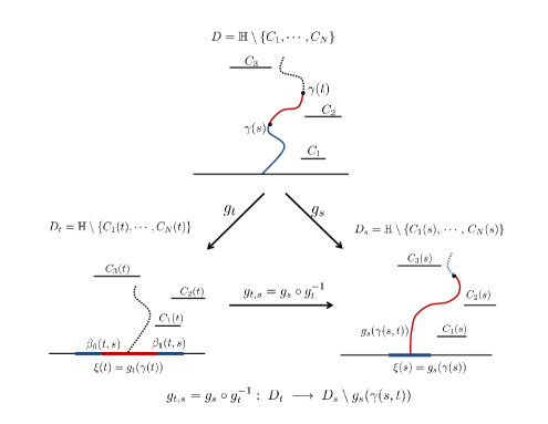
Figure 2: Conformal mapping $g_{t,s}$

We know from [CFR, (6.22)] that

$$g_{s}(z)-g_{t}(z)=\int_{\beta_{0}(t,s)}^{\beta_{1}(t,s)}\Psi_{t}(g_{t}(z),x)\Im g_{t,s}(x)dx.$$ (2.5)

Taking derivative in $z$ yields

$$(g_{s}^{\pm})^{\prime}(z)-(g_{t}^{\pm})^{\prime}(z)=\int_{\beta_{0}(t,s)}^{\beta_{1}(t,s)}(\eta^{\pm}_{t}(z,x))^{\prime}\,\Im g_{t,s}(x)dx.$$

On the other hand, it is established in [CFR, Lemma 6.2] that for $0\leq s<t<t_{\gamma}$ that

$$2(s-t)=a_{t}-a_{s}=\frac{1}{\pi}\int_{\beta_{0}(t,s)}^{\beta_{1}(t,s)}\Im g_{t,s}(x+i0+)dx.$$ (2.6)

Taking quotient of the last two displays and then passing $s\uparrow t$ yields

$$\partial_{t}^{-}(g_{t}^{\pm})^{\prime}(z)=-2\pi(\eta^{\pm}_{t}(z,\xi(t)))^{\prime},$$ (2.7)

where $\partial_{t}^{-}$ denotes the left-derivative in $t$. In view of (2.1) and the property (P.3), the right hand side of (2.7) is continuous in $t\in[0,t_{\gamma})$. Thus, as in the proof of [CFR, Thoerem 9.9], $(g_{t}^{\pm})^{\prime}(z)$ is differentiable in $t$. Consequently, (2.2) follows in view of (2.7).

(iv) Let $\widetilde{\gamma}$ be a closed smooth Jordan curve in $B({\bf 0},\sqrt{\varepsilon}).$ By Cauchy’s integral formula

$$(f_{t}^{\ell})^{\prime}(z)=\frac{1}{2\pi i}\int_{\eta}\frac{f_{t}^{\ell}(\zeta)}{(\zeta-z)^{2}}d\zeta,\quad z\in{\rm ins}\ \widetilde{\gamma}.$$

Since $f_{t}^{\ell}(\zeta)=g_{t}(\zeta^{2}+z_{j})$ is continuous in $t$ uniformly in $\zeta\in\widetilde{\gamma}$ by (P.1), we get the desired continuity. The same is true for $(f^{\ell}_{t})^{\prime\prime}(z).$

(v) Since $\Im\widetilde{\eta}_{t}(z,\zeta)$ is constant in $z$ on $B({\bf 0},\sqrt{\varepsilon})\cap\partial{\mathbb{H}}\setminus\{{\bf 0}\}$, it extends analytically to $B({\bf 0},\sqrt{\varepsilon})\setminus\{{\bf 0}\}$ by the Schwarz reflection. Note that ${\bf 0}$ is a removable singularity because $\Im\eta_{t}(z,\zeta)$ is bounded near $\{{\bf 0}\}$. The second assertion can be shown as the proof of (ii) using (P.1) and (P.5).

(vi) Taking $z$ to be $\psi^{-1}(z)$ in (2.5), we have

$$f_{s}^{\ell}(z)-f_{t}^{\ell}(z)=\int_{\beta_{0}(t,s)}^{\beta_{1}(t,s)}\widetilde{\eta}_{t}(z,x)\Im g_{t,s}(x)dx\quad\hbox{for }z\in B({\bf 0},\sqrt{\varepsilon})\hbox{ and }s<t.$$

Differentiating in $z$ gives

$$(f_{s}^{\ell})^{\prime}(z)-(f_{t}^{\ell})^{\prime}(z)=\int_{\beta_{0}(t,s)}^{\beta_{1}(t,s)}(\widetilde{\eta}_{t}(z,x))^{\prime}\Im g_{t,s}(x)dx\quad\hbox{for }z\in B({\bf 0},\sqrt{\varepsilon})\hbox{ and }s<t.$$

Taking quotient of the above with (2.6) and passing $s\uparrow t$ yields $\partial_{t}^{-}(f_{t}^{\ell})^{\prime}(z)=2\pi(\widetilde{\eta}_{t}(z,\xi(t)))^{\prime}.$ Since the right hand side is continuous in $t$ by (2.3) and (P.3), we arrive at the conclusion (vi). $\Box$

Denote by $z_{j}(t)$ and $z^{r}_{j}(t)$ the left and right endpoints of the slit $C_{j}(t)$, where $1\leq j\leq N$, for $D_{t}\in{\cal D}$ and $t\in[0,t_{\gamma})$. Since $g_{t}$ is a homeomorphism between $\partial_{p}C_{j}$ and $\partial_{p}C_{j}(t)$, for each $t\in[0,t_{\gamma})$ and $1\leq j\leq N$, there exist unique

$$\widetilde{z}_{j}(t)=\widetilde{x}_{j}(t)+iy_{j}\in\partial_{p}C_{j}\quad\hbox{and}\quad\widetilde{z}_{j}^{r}(t)=\widetilde{x}_{j}^{r}(t)+iy_{j}\in\partial_{p}C_{j}$$

so that $g_{t}(\widetilde{z}_{j}(t))=z_{j}(t)$ and $g_{t}(\widetilde{z}_{j}^{r}(t))=z_{j}^{r}(t)$.

Lemma 2.2

(i) If $\widetilde{z}_{j}(t)\in C_{j}^{+}\setminus\{z_{j},z_{j}^{r}\},$ then

$$(g_{t}^{+})^{\prime}(\widetilde{z}_{j}(t))=0,\qquad(g_{t}^{+})^{\prime\prime}(\widetilde{z}_{j}(t))\neq 0.$$ (2.8)

(ii) If $\widetilde{z}_{j}(t)\in C_{j}^{-}\setminus\{z_{j},z_{j}^{r}\},$ then (2.8) holds with $g_{t}^{-}$ in place of $g_{t}^{+}.$

(iii) If $\widetilde{z}_{j}(t)\in\partial_{p}C_{j}\cap B(z_{j},\varepsilon),$ then, for $\psi(z)=(z-z_{j})^{1/2},$

$$(f_{t}^{\ell})^{\prime}(\psi(\widetilde{z}_{j}(t)))=0,\qquad(f_{t}^{\ell})^{\prime\prime}(\psi(\widetilde{z}_{j}(t)))\neq 0.$$ (2.9)

(iv) If $\widetilde{z}_{j}(t)\in\partial_{p}C_{j}\cap B(z_{j}^{r},\varepsilon),$ then, for $\psi(z)=(z-z_{j}^{r})^{1/2},$

$$(f_{t}^{r})^{\prime}(\psi(\widetilde{z}_{j}(t)))=0,\qquad(f_{t}^{r})^{\prime\prime}(\psi(\widetilde{z}_{j}(t)))\neq 0.$$ (2.10)

(v) The above four statements also hold for $\widetilde{z}_{j}^{r}(t)$ in place of $\widetilde{z}_{j}(t).$

Proof. It suffices to prove (i) and (iii). $g_{t}^{+}$ is analytic on $R$ and $\widetilde{z}_{j}(t)\in R.$ Suppose $g_{t}^{+}(z)-z_{j}(t)$ has a zero of order $m$ at $\widetilde{z}_{j}(t)$: for some analytic function $h$ with $h(\widetilde{z}_{j}(t))\neq 0,$

$$g_{t}^{+}(z)-z_{j}(t)=g_{t}^{+}(z)-g_{t}^{+}(\widetilde{z}_{j}(t))=(z-\widetilde{z}_{j}(t))^{m}h(z).$$

Then, in view of [A, p131, Th.11], there exists $\varepsilon_{0}>0$ with $B(\widetilde{z}_{j}(t),\varepsilon_{0})\subset R$ and $\delta_{0}>0,$ such that, for any $w\in B(z_{j}(t),\delta_{0})$, $(g_{t}^{+})^{-1}(w)\cap B(\widetilde{z}_{j}(t),\varepsilon_{0})$ consists of $m$ distinct points. Since $g_{t}$ is homeomorphic between $\partial_{p}C_{j}$ and $\partial_{p}C_{j}(t),$ there exists $\delta_{00}>0$ such that, for any $\delta\in(0,\delta_{00})$ and for any $w\in B(z_{j}(t),\delta)\cap C_{j}(t)$ with $w\neq z_{j}(t),$ $(g_{t}^{+})^{-1}(w)\subset B(\widetilde{z}_{j}(t),\varepsilon_{0})\cap C_{j}^{+}$ consists of two points because $z_{j}(t)$ is an endpoint of $C_{j}(t)$ and so $w$ corresponds to two distinct points of $\partial_{p}C_{j}(t).$ Hence $m=2.$

(iii) Except for the last part, the following proof is similar to that of (i).

$f_{t}^{\ell}$ is analytic on $B({\bf 0},\sqrt{\varepsilon})$ and $\psi(\widetilde{z}_{j}(t))\in B({\bf 0},\sqrt{\varepsilon}).$ Suppose $f_{t}^{\ell}(z)-z_{j}(t)$ has a zero of order $m$ at $\psi(\widetilde{z}_{j}(t))$: for some analytic function $h$ with $h(\psi(\widetilde{z}_{j}(t)))\neq 0,$

$$f_{t}^{\ell}(z)-z_{j}(t)=f_{t}^{\ell}(z)-f_{t}^{\ell}(\psi(\widetilde{z}_{j}(t)))=(z-\psi(\widetilde{z}_{j}(t)))^{m}h(z),\ z\in B({\bf 0},\sqrt{\varepsilon}).$$

Then, as in the proof of (i), there exists $\varepsilon_{0}>0$ with $B(\psi(\widetilde{z}_{j}(t)),\varepsilon_{0})\subset B({\bf 0},\sqrt{\varepsilon})$ and $\delta_{0}>0,$ such that, for any $w\in B(z_{j}(t),\delta_{0})$, $(f_{t}^{\ell})^{-1}(w)\cap B(\psi(\widetilde{z}_{j}(t)),\varepsilon_{0})$ consists of $m$ distinct points. Since $z_{j}(t)$ is the endpoint of $C_{j}(t)$ and $g_{t}$ is homeomorphic between $\partial_{p}C_{j}$ and $\partial_{p}C_{j}(t),$ there exists $\delta_{00}>0$ such that, for any $\delta\in(0,\delta_{00})$ and for any $w\in B(z_{j}(t),\delta)\cap C_{j}(t)$ with $w\neq z_{j}(t),$ $(g_{t})^{-1}(w)\subset\partial_{p}C_{j}\cap B(z_{j},\varepsilon)$ consists of two points. In fact, $w$ corresponds to two distinct points $w_{+}\in C_{j}^{+}(t),\;w_{-}\in C_{j}^{-}(t)$ so that $g_{t}^{-1}(w)=\{\widetilde{w}_{+},\widetilde{w}_{-}\}$ with $g_{t}(\widetilde{w}_{\pm})=w_{\pm}.$ Then $(f_{t}^{\ell})^{-1}(w)=\psi(g_{t}^{-1}(w))=\{\psi(\widetilde{w}_{+}),\psi(\widetilde{w}_{-})\}$ consists of two distinct points of $B({\bf 0},\sqrt{\varepsilon}).$ Therefore $m=2.$ $\Box$

We let $h(t,z)=(g_{t}^{+})^{\prime}(z).$ Then $h(t,z)$ is a $C^{1}$-function in $(t,z)\in(0,t_{\gamma})\times R$ by virtue of Lemma 2.1.

Assume that $\widetilde{z}_{j}(t_{0})\in C_{j}^{+}\setminus\{z_{j},z_{j}^{r}\}.$ By (2.8),

$$h(t,\widetilde{z}_{j}(t))=0\qquad\hbox{for }t\in(t_{0}-\delta_{1},t_{0}+\delta_{1})$$ (2.11)

for some $\delta_{1}>0$. On the other hand, $|h^{\prime}(t,z)|=|(g_{t}^{+})^{\prime\prime}(z)|>0$ by Lemma 2.2. So by the implicit function theorem , there is some $\delta_{2}\in(0,\delta_{1})$ so that $t\mapsto\widetilde{z}_{j}(t)$ is $C^{1}$ in $t\in(t_{0}-\delta_{2},t_{0}+\delta_{2})$. Differentiating (2.11) in $t$ yields

$$\frac{d}{dt}\widetilde{z}_{j}(t)=-\frac{\partial_{t}h(t,z)}{h^{\prime}(t,z)}\Big{|}_{z=\widetilde{z}_{j}(t)}\qquad\hbox{for }t\in(t_{0}-\delta_{2},t_{0}+\delta_{2}).$$ (2.12)

The same assertions hold for $\widetilde{z}_{j}(t)$ when $\widetilde{z}_{j}(t)\in C_{j}^{-}\setminus\{z_{j},z_{j}^{r}\}$. A similar argument shows, by using (iii) and (iv) of Lemma 2.2, that $\psi(\widetilde{z}_{j}(t))$ is a $C^{1}$ function of $t$ in a neighborhood of $t_{0}$ when $\widetilde{z}_{j}(t_{0})\in\partial_{p}C_{j}\cap\left(B(z_{j},\varepsilon)\cup B(z_{j}^{r},\varepsilon)\right)$.

Theorem 2.3

The endpoints $z_{j}(t)=x_{j}(t)+iy_{j}(t),\ z_{j}^{r}(t)=x_{j}^{r}(t)+iy_{j}(t),$ of $C_{j}(t)$ satisfy the following equations for $1\leq j\leq N$:

$$\frac{d}{dt}y_{j}(t)=-2\pi\Im\Psi_{t}(z_{j}(t),\xi(t)),$$ (2.13)

$$\frac{d}{dt}x_{j}(t)=-2\pi\Re\Psi_{t}(z_{j}(t),\xi(t)),$$ (2.14)

$$\frac{d}{dt}x_{j}^{r}(t)=-2\pi\Re\Psi_{t}(z_{j}^{r}(t),\xi(t)).$$ (2.15)

Proof. It suffices to prove (2.13)-(2.14). It follows from (1.7) and (i), (iv) of Lemma 2.1 that

$$\partial_{t}g^{\pm}_{t}(z)=-2\pi\Psi_{t}(g^{\pm}_{t}(z),\xi(t))\quad\hbox{ for }z\in\partial_{p}C_{j}\setminus\{z_{j},z_{j}^{r}\}$$ (2.16)

and

$$\partial_{t}f^{\ell}_{t}(z)=-2\pi\Psi_{t}(f^{\ell}_{t}(z),\xi(t))\quad\hbox{ for }z\in\partial_{p}C_{j}\cap B(z_{j},\varepsilon).$$ (2.17)

Note that $z_{j}(t)=g^{\pm}_{t}(\widetilde{z}_{j}(t))$ when $\widetilde{z}_{j}(t)\in\partial_{p}C_{j}\setminus\{z_{j},z_{j}^{r}\}$ and $z_{j}(t)=f^{\ell}_{t}(\widetilde{z}_{j}(t))$ when $\widetilde{z}_{j}(t)\in\partial_{p}C_{j}\cap B(z_{j},\varepsilon)$. Since $\widetilde{z}_{j}(t)$ is $C^{1}$ in $t$, we have by Lemma 2.2

$$\frac{d}{dt}z_{j}(t)=\frac{d}{dt}(g^{\pm}_{t}(\widetilde{z}_{j}(t))=\partial_{t}g^{\pm}_{t}(\widetilde{z}_{j}(t))+(g^{\pm}_{t})^{\prime}(\widetilde{z}_{j}(t))\frac{d}{dt}\widetilde{z}_{j}(t)=-2\pi\Psi_{t}(z_{j}(t),\xi(t))$$

when $z_{j}(t)\in\partial_{p}C_{j}\setminus\{z_{j},z_{j}^{r}\}$, and

$$\frac{d}{dt}z_{j}(t)=\frac{d}{dt}f^{\ell}_{t}(\widetilde{z}_{j}(t))=\partial_{t}f^{\ell}_{t}(\widetilde{z}_{j}(t))+(f^{\ell}_{t})^{\prime}(\widetilde{z}_{j}(t))\frac{d}{dt}\widetilde{z}_{j}(t)=-2\pi\Psi_{t}(z_{j}(t),\psi(t))$$

when $z_{j}(t)\in\partial_{p}C_{j}\cap B(z_{j},\varepsilon)$. This proves (2.13)-(2.14). $\Box$

Remark 2.4

(i) The equation (2.13)-(2.15) was derived in [BF3] by assuming that $\widetilde{z}_{j}(t)\in\partial_{p}C_{j}\setminus\{z_{j},z_{j}^{r}\}$ and also by taking for granted the smoothness of  ‘$\frac{d}{dz}g_{t}(z)$’ in two variables $(t,z)$, which is now established by Lemma 2.1.

(ii) If

$$g_{t}(z_{j})=z_{j}(t)\ \hbox{ and }\ g_{t}(z_{j}^{r})=z_{j}^{r}(t)\qquad\hbox{for }t\in(0,t_{\gamma})\hbox{ and }1\leq j\leq N,$$ (2.18)

then Theorem 2.3 is merely a special case of the Komatu-Loewner equation (1.7) with $z=z_{j}$ and $z=z_{j}^{r}$, $1\leq j\leq N$, respectively. But in general (2.18) is not true. $\Box$

We call (2.13)-(2.15) the Komatu-Loewner equation for the slits.

3 Randomized curve $\gamma$ and induced process ${\bf W}$

3.1 Random curve with domain Markov property and a conformal invariance

As in the previous sections, for a standard slit domain $D={\mathbb{H}}\setminus\bigcup_{k=1}^{N}C_{k}$, the left and right endpoints of the $k$th slit $C_{k}$ are denoted by $z_{k}=x_{k}+iy_{k}$ and $z_{k}^{r}=x_{k}^{r}+iy_{k}^{r}$, respectively. Recall that ${\cal D}$ is the collection of all labeled (or, ordered) standard slits domains equipped with metric $d$ of (1.1). We define an open subset ${\cal S}$ of the Euclidean space ${\mathbb{R}}^{3N}$ by

$${\cal S} = \Big{\{}{\bf s}:=({\bf y},{\bf x},{\bf x}^{r})\in{\mathbb{R}}^{3N}:\ {\bf y},\;{\bf x},\>{\bf x}^{r}\in{\mathbb{R}}^{N},\ {\bf y}>{\bf 0},\ {\bf x}<{\bf x}^{r},$$ (3.1)

$$\hskip 21.68121pt{\rm either}\ x_{j}^{r}<x_{k}\ {\rm or}\ x_{k}^{r}<x_{j}\ {\rm whenever}\ y_{j}=y_{k},\ j\neq k\Big{\}}.$$

The Borel $\sigma$-field on ${\cal S}$ will be denoted as ${\mathscr{B}}({\cal S})$. The space ${\cal D}$ can be identified with ${\cal S}$ as a topological space. We write ${\bf s}(D)$ (resp. $D({\bf s})$) the element in ${\cal S}$ (resp. ${\cal D}$) corresponding to $D\in{\cal D}$ (resp. ${\bf s}\in{\cal S}$).

A set $F\subset{\mathbb{C}}$ is called an ${\mathbb{H}}$-hull if $\overline{F}$ is compact, $F=\overline{F}\cap{\mathbb{H}}$ and ${\mathbb{H}}\setminus F$ is simply connected. For $D\in{\cal D}$ and an ${\mathbb{H}}$-hull $F\subset D$, there exists a unique conformal map $g$ from $D\setminus F$ onto some $\widetilde{D}\in{\cal D}$ satisfying the hydrodynamic normalization $g(z)=z+\frac{a}{z}+o\left(\frac{1}{|z|}\right)$ as $z\to\infty.$ In what follows, such a map $g$ will be called a canonical map from $D\setminus F$. The associated constant $a$ (which is real and non-negative) will be called the half-plane capacity of $g$ and can be evaluated as

$$a=\lim_{z\to\infty}z(g(z)-z).$$ (3.2)

Set

$$\widehat{\cal D}=\{\widehat{D}=D\setminus F:\,D\in{\cal D}\hbox{ and }F\subset D\hbox{ is an }{\mathbb{H}}\hbox{-hull}\}.$$

For $\widehat{D}=D\setminus F\in\widehat{\cal D}$, let

$$\Omega(\widehat{D})=\left\{\gamma=\{\gamma(t):0\leq t<t_{\gamma}\}:\hbox{\rm Jordan arc},\ \gamma(0,t_{\gamma})\subset\widehat{D},\;\gamma(0)\in\partial({\mathbb{H}}\setminus F),\ 0<t_{\gamma}\leq\infty\right\}.$$

Two curves $\gamma,\;\widetilde{\gamma}\in\Omega(\widehat{D})$ are regarded equivalent if $\widetilde{\gamma}$ can be obtained from $\gamma$ by a reparametrization. Denote by $\dot{\Omega}(\widehat{D})$ the equivalence classes of $\Omega(\widehat{D})$.

Given $\gamma\in\Omega(\widehat{D})$ for $\widehat{D}=D\setminus F\in\widehat{\cal D},$ let $g_{t}$ be the canonical map from $\widehat{D}\setminus\gamma[0,t]=D\setminus(\gamma[0,t]\cup F)$ with the half-plane capacity $a_{t}$, $t\in[0,t_{\gamma})$. Note that $g_{t}=\widehat{g}_{t}\circ g$, where $g$ is the canonical map from $D\setminus F$ onto some $\widehat{D}\in{\cal D}$ and $\widehat{g}_{t}$ is the canonical map from $\widehat{D}\setminus g(\gamma[0,t])$ onto some $D_{t}\in{\cal D}$. It then follows from (3.2) that $a_{t}=a+\widehat{a}_{t}$, where $a$ and $\widehat{a}_{t}$ are the half-plane capacity of $g$ and $\widehat{g}_{t}$ respectively.

Since $\widehat{a}_{t}=a_{t}-a_{0}$ is strictly increasing and continuous in $t\in[0,t_{\gamma})$ with $\widehat{a}_{0}=0$ by (P.2), the curve $\gamma$ can be reparametrized as $\widetilde{\gamma}(t)=\gamma(\widehat{a}_{2t}^{-1})$ for $0\leq t<t_{\widetilde{\gamma}}:=\frac{1}{2}\widehat{a}_{t_{\gamma}}$ so that the corresponding half-plane capacity becomes $a_{0}+2t$. The curve $\widetilde{\gamma}$ is called the half-plane capacity renormalization of $\gamma.$

Throughout the rest of this paper, each $\dot{\gamma}\in\dot{\Omega}(\widehat{D})$ will be represented by a curve (denoted by $\dot{\gamma}$ again) belonging to this class parametrized by the half-plane capacity. We conventionally adjoin an extra point $\Delta$ to $\overline{\mathbb{H}}$ and define $\dot{\gamma}(t)=\Delta$ for $t\geq t_{\dot{\gamma}}$ so that $\dot{\gamma}$ can be regarded as a map from $[0,\infty]$ to $\overline{\mathbb{H}}\cup\{\Delta\}.$ We then introduce a filtration $\{\dot{\cal G}_{t}(\widehat{D});t\geq 0\}$ on $\dot{\Omega}(\widehat{D})$ by

$$\dot{\cal G}_{t}(\widehat{D}):=\left(\sigma\{\dot{\gamma}(s):\;0\leq s\leq t\}\right)\cap\{t<t_{\dot{\gamma}}\},\qquad\dot{\cal G}(\widehat{D}):=\sigma\{\dot{\gamma}(s):s\geq 0\}.$$

For each $D\in{\cal D}$, we consider a family of probability measures $\{{\mathbb{P}}_{D,z};\,z\in\partial{\mathbb{H}}\}$ on $(\dot{\Omega}(D),\dot{\cal G}(D))$ that satisfies the property

$${\mathbb{P}}_{D,z}(\{\dot{\gamma}(0)=z\})=1,\qquad z\in\partial{\mathbb{H}},$$ (3.3)

as well as the following (DMP) and (IL).

For each $\widehat{D}\in\widehat{\cal D}$ and $t\geq 0,$ define the shift operator $\dot{\theta}_{t}:\dot{\Omega}(\widehat{D})\cap\{t<t_{\dot{\gamma}}\}\mapsto\dot{\Omega}(\widehat{D}\setminus\dot{\gamma}[0,t])$ by

$$(\dot{\theta}_{t}\dot{\gamma})(s)=\dot{\gamma}(t+s)\qquad\hbox{for }s\in[0,t_{\dot{\gamma}}-t).$$ (3.4)

(DMP) (Domain Markov property): for any $D\in{\cal D}$, $t\geq 0$ and $z\in\partial{\mathbb{H}}$,

$${\mathbb{P}}_{D,z}\left(\dot{\theta}_{t}^{-1}\Lambda\big{|}\dot{\cal G}_{t}(D)\right)={\mathbb{P}}_{g_{t}(D\setminus\dot{\gamma}[0,t]),g_{t}(\dot{\gamma}(t))}(g_{t}(\Lambda))\quad\hbox{for every }\Lambda\in\dot{\cal G}(D\setminus\dot{\gamma}[0,t]).$$ (3.5)

Here $g_{t}(z)$ is the canonical map from $D\setminus\dot{\gamma}[0,t]$. Note that $g_{t}(D\setminus\dot{\gamma}[0,t])\in{\cal D}$ and $g_{t}(\dot{\gamma}(t))\in\partial{\mathbb{H}}$ is well-defined since $g_{t}(z)$ can be extended continuously to $\partial_{p}(D\setminus\dot{\gamma}[0,t])$.

(IL) (Invariance under linear conformal map): for any $D\in{\cal D}$ and any linear map $f$ from $D$ onto $f(D)\in{\cal D}$,

$${\mathbb{P}}_{f(D),f(z)}={\mathbb{P}}_{D,z}\circ f^{-1}\qquad\hbox{for every }z\in\partial{\mathbb{H}}.$$ (3.6)

Remark 3.1

For $\widehat{D}=D\setminus F\in\widehat{\cal D}$, let $\Phi$ be the canonical map that maps $\widehat{D}$ onto $\Phi(\widehat{D})\in{\cal D}$. Suppose that $\Phi$ can be extended continuously to $\partial_{p}({\mathbb{H}}\setminus F)$. Then for each $z\in\partial_{p}({\mathbb{H}}\setminus F)$, one can define ${\mathbb{P}}_{\widehat{D},z}={\mathbb{P}}_{\Phi(\widehat{D}),\Phi(z)}\circ\Phi^{-1}$. We can therefore restate (3.5) as

$${\mathbb{P}}_{D,z}\left(\dot{\theta}_{t}^{-1}\Lambda\big{|}\dot{\cal G}_{t}(D)\right)={\mathbb{P}}_{D\setminus\dot{\gamma}[0,t],\dot{\gamma}(t)}(\Lambda)\quad\hbox{for every }\Lambda\in\dot{\cal G}(D\setminus\dot{\gamma}[0,t]).$$ (3.7)

This explains why we call (3.5) the domain Markov property. The formulation (3.5) avoids the technical issue whether $\Phi$ can be extended continuously to $\partial_{p}({\mathbb{H}}\setminus F)$ for general $\widehat{D}=D\setminus F\in\widehat{\cal D}$. See Proposition 5.10 and Theorem 5.11 in Section 5. $\Box$

3.2 Markov property of ${\bf W}$

For each $D\in{\cal D},\ \dot{\gamma}\in\dot{\Omega}(D)$ and $t\in[0,t_{\dot{\gamma}}),$ $\dot{\gamma}$ induces the conformal map $g_{t}$ from $D\setminus\dot{\gamma}[0,t]$ onto $D_{t}=g_{t}(D)\in{\cal D}.$ The conformal map $g_{t}(z)$ can be extended to a continuous map from $D\cup\partial_{p}K\cup\partial_{p}\gamma[0,t]\cup\partial{\mathbb{H}}$ onto $\overline{\mathbb{H}}$. We occasionally write $g_{t}$ as $g_{t}^{D}$ or $g_{D\setminus\dot{\gamma}[0,t]}$ to indicate its dependence on $\dot{\gamma}\in\dot{\Omega}(D)$. Note that $g_{t}$ sends $\dot{\gamma}(t)$ to $\xi(t)\in\partial{\mathbb{H}}$.

Let $\{{\bf s}(t)={\bf s}(D_{t}),\;t\in[0,t_{\dot{\gamma}})\}$ be the induced slit motion with $D_{0}:=D$. We will consider the joint process

$${\bf W}_{t}=\left\{\begin{array}[]{ll}(\xi(t),{\bf s}(t))\in{\mathbb{R}}\times S\subset{\mathbb{R}}^{3N+1},&\quad 0\leq t<t_{\dot{\gamma}},\\ \delta,&\quad t\geq t_{\dot{\gamma}}.\end{array}\right.$$

Here the real part of $\xi(t)\in\partial{\mathbb{H}}$ is designated by $\xi(t)$ again and $\delta$ is an extra point conventionally adjoined to ${\mathbb{R}}\times S.$ We shall occasionally write ${\bf s}(t)$ as $g_{t}^{D}({\bf s})$ with ${\bf s}={\bf s}(D).$

To establish the Markov property of ${\bf W}_{t}$, we need the following measurability results.

Lemma 3.2

Fix $D\in{\cal D}$ and $t\geq 0.$

(i) For each $z\in D$, $\Im g_{t}(z)$ is a $[0,\infty)$-valued $\dot{\cal G}_{t}(D)$-measurable function on $\dot{\Omega}(D).$

(ii) $g_{t}(z)$ is an $\overline{\mathbb{H}}$-valued ${\mathscr{B}}(D\cup\partial_{p}K\cup\partial_{p}\dot{\gamma}[0,t]\cup\partial{\mathbb{H}})\times\dot{\cal G}_{t}(D)$-measurable function on $(D\cup\partial_{p}K\cup\partial_{p}\dot{\gamma}[0,t]\cup\partial{\mathbb{H}})\times\dot{\Omega}(D).$

(iii) ${\bf W}_{t}$ is an ${\mathbb{R}}^{3N+1}$-valued $\dot{\cal G}_{t}(D)$-measurable function on $\dot{\Omega}(D).$

Proof.  (i) We make use of the probabilistic representation (1.6) of $\Im g_{t}(z).$  Take $r>0$ such that the set ${\mathbb{H}}_{r}=\{z\in{\mathbb{H}}:\Im z<r\}$ contains $\dot{\gamma}(0,t]\cup K.$  It suffices to show $F_{z,r}(\dot{\gamma})={\mathbb{P}}_{z}^{{\mathbb{H}},*}(\sigma_{\Gamma_{r}}<\sigma_{\dot{\gamma}(0,t]})$ is a $\dot{\cal G}_{t}(D)$-measurable function on $\dot{\Omega}(D)$ for each fixed $z\in D.$

Let $Z^{{\mathbb{H}}_{r},*}=(Z_{t}^{{\mathbb{H}}_{r},*},\zeta,{\mathbb{P}}_{z}^{{\mathbb{H}}_{r},*})$ be the BMD on ${\mathbb{H}}_{r}^{*}=(D\cap{\mathbb{H}}_{r})\cup\{c_{1}^{*},\cdots,c_{N}^{*}\}$ obtained from the absorbing Brownian motion on ${\mathbb{H}}_{r}$ by rendering each hole $C_{k}$ into a single point $c_{k}^{*}$, with life time $\zeta$. Then

$$F_{z,r}(\dot{\gamma})={\mathbb{P}}_{z}^{{\mathbb{H}}_{r},*}(\sigma_{\dot{\gamma}(0,t]}=\infty)={\mathbb{P}}_{z}^{{\mathbb{H}}_{r},*}(\dot{\gamma}(0,t]\cap Z_{[0,\zeta)}^{{\mathbb{H}}_{r},*}=\emptyset).$$ (3.8)

Let ${\mathbb{H}}_{r}^{*}\cup\{\Delta\}$ be the one-point compactification of ${\mathbb{H}}_{r}^{*}.$. As the sample space $(\Xi,{\mathscr{B}}(\Xi))$ of $Z^{{\mathbb{H}}_{r},*}$, we take

$$\Xi=\{Z\in C([0,\infty)\mapsto{\mathbb{H}}_{r}^{*}\cup\{\Delta\}):Z_{t}=\Delta,\ t\geq\zeta(=\sigma_{\Delta})\}$$

and ${\mathscr{B}}(\Xi)=\sigma\{Z_{t},t\geq 0\}.$ We consider the direct product $\dot{\Omega}(D)\times\Xi$ of the measurable space $(\dot{\Omega}(D),\dot{\cal G}_{t}(D))$ and $(\Xi,{\mathscr{B}}(\Xi)).$  Then the set $\Lambda=\{(\dot{\gamma},Z)\in\dot{\Omega}(D)\times\Xi:\dot{\gamma}(0,t]\cap Z_{[0,\infty)}=\emptyset\}$ is $\dot{\cal G}_{t}(D)\times{\mathscr{B}}(\Xi)$-measurable because

$$\Lambda=\bigcup_{n=1}^{\infty}\bigcap_{u\in[0,t]\bigcap{\mathbb{Q}}_{+}}\bigcap_{v\in{\mathbb{Q}}_{+}}\{|\dot{\gamma}(u)-Z_{v}|>1/n\},$$

where ${\mathbb{Q}}_{+}$ denotes the set of positive rational numbers.

In view of (3.8), $F_{z,r}(\dot{\gamma})={\mathbb{P}}_{z}^{{\mathbb{H}}_{r},*}(\Lambda_{\dot{\gamma}})$ for the $\dot{\gamma}$-section $\Lambda_{\dot{\gamma}}=\{Z\in\Xi:(\dot{\gamma},Z)\in\Lambda\}$ of $\Lambda$ and so $F_{z,\gamma}(\dot{\gamma})$ is $\dot{\cal G}_{t}(D)$-measurable by the Fubini Theorem.

(ii) By (i) and (1.6), $\Im g_{t}(z)=\lim_{r\to\infty}rF_{z,r}(\dot{\gamma})$ is $\dot{\cal G}_{t}(D)$-measurable in $\dot{\gamma}$ for each $z\in D$. On the other hand, it is continuous in $z\in D\cup\partial_{p}K\cup\partial_{p}\dot{\gamma}[0,t]\cup\partial{\mathbb{H}}$ for each $\dot{\gamma}\in\dot{\Omega}(D).$ Therefore $\Im g_{t}$ is ${\mathscr{B}}(D\cup\partial_{p}K\cup\partial_{p}\dot{\gamma}[0,t]\cup\partial{\mathbb{H}})\times\dot{\cal G}_{t}(D)$-measurable in $(z,\dot{\gamma}).$

Since $g_{t}$ is obtained from $\Im g_{t}$ explicitly via [CFR, (10.17)], $g_{t}$ enjoys the same joint measurability.

(iii) This follows from (ii). $\Box$

For $\xi\in{\mathbb{R}}$ and ${\bf s}\in S$, we denote the probability measure ${\mathbb{P}}_{D({\bf s}),\xi+i0}$ on $(\dot{\Omega}(D({\bf s})),\dot{\cal G}(D({\bf s})))$ by ${\mathbb{P}}_{(\xi,{\bf s})}$.

Theorem 3.3

(Time homogeneous Markov property) The process $\{{\bf W}_{t},t\geq 0;{\mathbb{P}}_{(\xi,{\bf s})},\,\xi\in{\mathbb{R}},\,{\bf s}\in{\cal S}\}$ is $\{\dot{\cal G}_{t}(D({\bf s}(0));t\geq 0\}$-adapted, and

$${\mathbb{P}}_{(\xi,{\bf s})}({\bf W}_{0}=(\xi,{\bf s}))=1,$$ (3.9)

$${\mathbb{P}}_{(\xi,{\bf s})}\left({\bf W}_{t+s}\in B\;\big{|}\;\dot{\cal G}_{t}(D({\bf s}))\right)={\mathbb{P}}_{{\bf W}_{t}}({\bf W}_{s}\in B)\quad\hbox{for }t,s\geq 0,\ B\in\mathscr{B}({\mathbb{R}}\times{\cal S}).$$ (3.10)

Proof.  ${\bf W}_{t}$ is $\dot{\cal G}_{t}(D({\bf s}(0))$-measurable by Lemma 3.2. (3.9) follows from (3.3).

For $D=D({\bf s})\in{\cal D}$, $\dot{\gamma}\in\dot{\Omega}(D)$ and $t\in[0,t_{\dot{\gamma}})$, $g_{t}^{D}$ is a conformal map from $D\setminus\dot{\gamma}[0,t]\in\widehat{\cal D}$ onto $D_{t}\in{\cal D}$ sending $\dot{\gamma}(t)$ to $\xi(t)\in\partial{\mathbb{H}}$ and so, by (3.5), for $\Lambda\in\dot{\cal G}(D\setminus\dot{\gamma}[0,t])$ and $z\in\partial{\mathbb{H}}$

$${\mathbb{P}}_{D,z}(\dot{\theta}_{t}^{-1}\Lambda\;\big{|}\;\dot{\cal G}_{t}(D))={\mathbb{P}}_{D_{t},\xi(t)}(g_{t}^{D}(\Lambda)).$$ (3.11)

Set, for $t,s\geq 0$ and $B\in{\mathscr{B}}({\mathbb{R}}\times{\cal S}),$

$$\Lambda_{t,s}=\left\{\dot{\eta}\in\dot{\Omega}(D\setminus\dot{\gamma}[0,t]):\dot{\eta}(0)=\dot{\gamma}(t),\ (\widehat{\xi}(s),\widehat{\bf s}(s))\in B\right\}.$$

Here, by means of the canonical (conformal) map $g^{D\setminus\dot{\gamma}[0,t]}_{s}$ from $(D\setminus\dot{\gamma}[0,t])\setminus\dot{\eta}[0,s]$ onto $\widehat{D}_{s}\in{\cal D}$, we define $\widehat{\xi}(s)=g^{D\setminus\dot{\gamma}[0,t]}_{s}(\dot{\eta}(s))$ and $\widehat{\bf s}(s)={\bf s}(\widehat{D}_{s})$. Then we have

$$\theta^{-1}_{t}\Lambda_{t,s}=\{\dot{\gamma}\in\dot{\Omega}(D):{\bf W}_{t+s}\in B\}\quad\hbox{and}\quad g^{D}_{t}(\Lambda_{t,s})=\left\{\dot{\gamma}\in\dot{\Omega}(D_{t}):\dot{\gamma}(0)=\xi(t),\ {\bf W}_{s}\in B\right\}.$$

In fact, the first identity is due to the relation

$$g^{D}_{t+s}(z)=g_{D_{t}\setminus g^{D}_{t}\dot{\gamma}[t,t+s]}\circ g^{D}_{t}(z),$$

while the second one is obtained by the observation that $g^{D}_{t}$ induces a one-to-one map between $\dot{\Omega}(D\setminus\dot{\gamma}[0,t])$ and $\dot{\Omega}(D_{t}).$

The conclusion of the theorem now follows from (3.11). $\Box$

Remark 3.4

The filtration $\{\dot{\cal G}_{t}(D({\bf s})),\;t\geq 0\}$ in the identity (3.10) depends on the second component ${\bf s}$ of the initial state $(\xi,{\bf s}).$ Nevertheless we can regard the process $({\bf W}_{t},{\mathbb{P}}_{(\xi,{\bf s})})$ as a Markov process on ${\mathbb{R}}\times{\cal S}$ in a usual sense. If we write ${\bf w}=(\xi,{\bf s})$ and introduce a transition function $P_{t}$ on ${\mathbb{R}}\times{\cal S}$ by

$$P_{t}f({\bf w})={\mathbb{E}}_{\bf w}[f({\bf W}_{t})],\quad f\in{\mathscr{B}}_{b}({\mathbb{R}}\times{\cal S}),$$

then (3.10) implies that, for any $0\leq t_{1}<t_{2}<\cdots<t_{n}$, $f_{1},f_{2},\cdots,f_{n}\in{\mathscr{B}}_{b}({\mathbb{R}}\times{\cal S})$, and ${\bf w}\in{\mathbb{R}}\times{\cal S}$,

$${\mathbb{E}}_{\bf w}\left[\prod_{k=1}^{n}f_{k}({\bf W}_{t_{k}})\right]=\int_{({\mathbb{R}}\times{\cal S})^{n}}\prod_{k=1}^{n}f_{k}({\bf w}_{k})P_{t_{k}-{t_{k-1}}}({\bf w}_{k-1},d{\bf w}_{k})$$

with $t_{0}:=0$ and ${\bf w}_{0}:=w$. $\Box$

3.3 Brownian scaling for ${\bf W}$

Lemma 3.5

For $D\in{\cal D},\gamma\in\Omega(D),$ let $a_{t}=a_{t}(\gamma,D)$ be the associated half-plane capacity. Then for any $c>0$

$$a_{t}(c\gamma,cD)=c^{2}a_{t}(\gamma,D),\quad t\in[0,t_{\gamma}).$$ (3.12)

In particular, if $\gamma$ is parameterized by the half-plane the half-plane capacity, then

$$\left(\dot{c\gamma}\right)(t)=c\;\dot{\gamma}(c^{-2}t),\quad 0\leq t<c^{2}t_{\dot{\gamma}}=:t_{\dot{(c\gamma)}}.$$ (3.13)

is the half-plane capacity parametrization of the curve $c\gamma$ in $cD$.

Proof.  Let $g_{t}(z)$ be the canonical map from $D\setminus\gamma.$ Then $g_{t}^{c}(z)=cg_{t}(z/c)$ is the canonical map from $cD\setminus c\gamma.$ (3.12) follows from (3.2) and

$$z(g_{t}^{c}(z)-z)=c^{2}\frac{z}{c}\left(g_{t}(\frac{z}{c})-\frac{z}{c}\right).$$

(3.13) follows from $a_{t}(\dot{\gamma},D)=2t$ and (3.12). $\Box$

We make a convention that $c\;\Delta=\Delta$ for any constant $c>0.$ Then the identity (3.13) holds for any $t\geq 0$; for $t\geq c^{2}t_{\dot{\gamma}},$ the both hand sides of (3.13) equal $\Delta.$ Keeping this in mind, we show the following:

Proposition 3.6

For $D\in{\cal D},\;z\in\partial{\mathbb{H}}$ and any $c>0$

$$\{c^{-1}\dot{\gamma}(c^{2}t),\;t\geq 0\}\ {\rm under}\ {\mathbb{P}}_{cD,cz}\ \hbox{ has the same distribution as }\ \{\dot{\gamma}(t),\;t\geq 0\}\ {\rm under}\ {\mathbb{P}}_{D,z}.$$ (3.14)

Proof.  For a fixed $c>0$, $f(z)=cz$ is a conformal map from $D$ onto $cD\in{\cal D}$. By the invariance under linear conformal map (3.6), we have for $D\in{\cal D},\ z\in\partial{\mathbb{H}}$

$${\mathbb{P}}_{D,z}(\Lambda)=f^{-1}_{*}{\mathbb{P}}_{cD,cz}(\Lambda)={\mathbb{P}}_{cD,cz}(f(\Lambda)),\quad\Lambda\in\dot{\cal G}(D).$$ (3.15)

For $\Lambda=\{\dot{\gamma}\in\dot{\Omega}(D):\dot{\gamma}\in B\}\in\dot{\cal G}(D)$ with $B\in{\mathscr{B}}\left((\overline{\mathbb{H}}\cup\{\Delta\})^{[0,\infty)}\right)$, $f(\Lambda)=\{\dot{\gamma}\in\dot{\Omega}(cD):\dot{(\gamma/c)}\in B\}$. By (3.13),

$$\dot{(\gamma/c)}(t)=c^{-1}\dot{\gamma}(c^{2}t),\quad t\geq 0,$$ (3.16)

and so (3.14) follows from (3.15). $\Box$

Theorem 3.7

(Brownian scaling property of ${\bf W}$)  For $\xi\in{\mathbb{R}}$, ${\bf s}\in{\cal S}$ and $c>0$

$$\{c^{-1}{\bf W}_{c^{2}t},\;t\geq 0\}\ {\rm under}\ {\mathbb{P}}_{(c\xi,c{\bf s})}\ \hbox{ has the same distribution as }\ \{{\bf W}_{t},\;t\geq 0\}\ {\rm under}\ {\mathbb{P}}_{(\xi,{\bf s})}.$$ (3.17)

Proof.  For fixed $D\in{\cal D}$ and $c>0,$ consider the canonical map $g_{t}^{cD}$ associated with $cD$ and a curve $\{\dot{\gamma}(t),\;t\geq 0\}\subset\dot{\Omega}(cD).$ The induced process ${\bf W}_{t}=(\xi(t),{\bf s}(t))$, $t\in[0,t_{\dot{\gamma}})$, is given by ${\bf s}(t)=g_{t}^{cD}(c{\bf s})$ for ${\bf s}={\bf s}(D)$ and $\xi(t)=g_{t}^{cD}(\dot{\gamma}(t)).$

Now the curve on the left hand side of (3.14) defined for $\dot{\gamma}\in\dot{\Omega}(cD)$ belongs to $\dot{\Omega}(D)$ in view of (3.16) and the associated canonical map $\widetilde{g}_{t}^{D}$ from $D$ is given by

$$\widetilde{g}_{t}^{D}(z)=c^{-1}g_{c^{2}t}^{cD}(cz),\quad z\in D,\quad{\rm for}\ t\in[0,t_{\dot{\gamma}/c^{2}}),$$ (3.18)

which induces the motion $\{c^{-1}{\bf W}_{c^{2}t}:\ t\in[0,t_{\dot{\gamma}/c^{2}})\},$ because $\widetilde{g}_{t}^{D}({\bf s})=c^{-1}{\bf s}(c^{2}t)$ and $\widetilde{g}_{t}^{D}(c^{-1}\dot{\gamma}(c^{2}t))=c^{-1}\xi(c^{2}t)$ for $t\in[0,t_{\dot{\gamma}/c^{2}})$.

Let $\{{\bf W}_{t},\;t\geq 0\}$ be the $({\mathbb{R}}\times S)$-valued motion produced by $D\in{\cal D}$ and $\dot{\gamma}\in\dot{\Omega}(D).$ Then, for $0\leq t_{1}<t_{2}<\cdots<t_{n}$, $({\bf W}_{t_{1}},{\bf W}_{t_{2}},\cdots,{\bf W}_{t_{n}})$ equals an $({\mathbb{R}}\times S)^{n}$-valued $\dot{\cal G}(D)$-measurable function $F(\dot{\gamma})$ of $\dot{\gamma}\in\dot{\Omega}(D)$ by virtue of Lemma 3.2. Therefore we can conclude from (3.14) and the above observation that (3.17) holds. $\Box$

3.4 Homogeneity of ${\bf W}$ in $x$-direction

Lemma 3.8

For $D\in{\cal D},\gamma\in\Omega(D),$ let $a_{t}=a_{t}(\gamma,D)$ be the associated half-plane capacity. Then for any ${r}\in{\mathbb{R}}$,

$$a_{t}(\gamma+{r},D+{r})=a_{t}(\gamma,D),\quad t\in[0,t_{\gamma}).$$ (3.19)

In particular, the half-plane capacity parametrization of the curve $\gamma+{r}$ in $D+{r}$ is given by $\dot{\gamma}+{r}$; in other words,

$$\dot{(\gamma+{r})}(t)=\dot{\gamma}(t)+{r},\quad 0\leq t<t_{\dot{\gamma}}.$$ (3.20)

Proof.  Let $g_{t}(z)$ be the canonical map associated with $(\gamma,D).$ Then $g_{t}^{r}(z)=g_{t}(z-{r})+{r}$ is the canonical map associated with $(\gamma+{r},D+{r}).$ (3.19) follows from (3.2) and

$$z(g_{t}^{r}(z)-z)=\frac{z}{z-{r}}\cdot(z-{r})\left(g_{t}(z-{r})-(z-{r})\right).$$

(3.20) follows from $a_{t}(\dot{\gamma},D)=2t$ and (3.19). $\Box$

The identity (3.20) holds for any $t\geq 0$ because both hand sides of (3.20) equal $\Delta$ when $t\geq t_{\dot{\gamma}}$.

Proposition 3.9

For $D\in{\cal D},\;z\in\partial{\mathbb{H}}$ and any ${r}\in{\mathbb{R}}$

$$\{\dot{\gamma}(t)-{r},\;t\geq 0\}\ {\rm under}\ {\mathbb{P}}_{D+{r},z+{r}}\ \hbox{ has the same distribution as }\ \{\dot{\gamma}(t),\;t\geq 0\}\ {\rm under}\ {\mathbb{P}}_{D,z}.$$ (3.21)

Proof.  For a fixed ${r}\in{\mathbb{R}}$, consider the sift $f(z)=z+{r},\quad z\in D$. By the invariance under linear conformal map (3.6), we have for $D\in{\cal D},\ z\in\partial{\mathbb{H}}$

$${\mathbb{P}}_{D,z}(\Lambda)=f^{-1}_{*}{\mathbb{P}}_{D+{r},z+{r}}(\Lambda)={\mathbb{P}}_{D+{r},z+{r}}(f(\Lambda)),\quad\Lambda\in\dot{\cal G}(D).$$ (3.22)

$\Lambda\in\dot{\cal G}(D)$ can be expressed as $\Lambda=\{\dot{\gamma}\in\dot{\Omega}(D):\dot{\gamma}\in B\}$ for $B\in{\mathscr{B}}\left((\overline{\mathbb{H}}\cup\{\Delta\})^{[0,\infty)}\right).$ Then

$$f(\Lambda)=\{\dot{\gamma}\in\dot{\Omega}(D+{r}):\dot{(\gamma-{r})}\in B\}.$$

This combined with (3.20) and (3.22) leads us to (3.21). $\Box$

For ${r}\in{\mathbb{R}},$ denote by $\widehat{r}$ the vector in ${\mathbb{R}}^{3N}$ whose first $N$ entries are $0$ and the last $2N$ entries are ${r}$. Note that ${\bf s}(D+{r})={\bf s}(D)+\widehat{r}\quad\hbox{ for }D\in{\cal D},\ {r}\in{\mathbb{R}}.$

Theorem 3.10

(Homogeneity of $({\bf W}_{t},\;{\mathbb{P}}_{(\xi,{\bf s})})$ in $x$-direction) For $\xi\in{\mathbb{R}}$, ${\bf s}\in S$ and ${r}\in{\mathbb{R}}$, $\{(\xi(t)-{r},{\bf s}(t)-\widehat{r}),\;t\geq 0\}$ under ${\mathbb{P}}_{(\xi+{r},{\bf s}+\widehat{r})}$ has the same distribution as $\{(\xi(t),{\bf s}(t)),\;t\geq 0\}$ under ${\mathbb{P}}_{(\xi,{\bf s})}$.

Proof.  Fixed $D\in{\cal D},\ z=\xi+i0\in\partial{\mathbb{H}}$, ${r}\in{\mathbb{R}}$ and put ${\bf s}={\bf s}(D).$ Consider the canonical map $g_{t}^{D+{r}}$ associated with $D+{r}$ and a curve $\{\dot{\gamma}(t),\;t\geq 0\}\subset\dot{\Omega}(D+{r}).$ The process ${\bf W}_{t}=({\bf s}(t),\xi(t)),\ t\in[0,t_{\dot{\gamma}}),$ being considered under ${\mathbb{P}}_{D+{r},z+{r}}={\mathbb{P}}_{(\xi+{r},{\bf s}+\widehat{r})}$ is induced from $g_{t}^{D+{r}}$ by

$$\xi(t)=g_{t}^{D+{r}}(\dot{\gamma}(t)),\quad{\bf s}(t)=g_{t}^{D+{r}}({\bf s}+\widehat{r}).$$

Now the curve on the left hand side of (3.21) belongs to $\dot{\Omega}(D)$ in view of (3.20) and the associated canonical map $\widetilde{g}_{t}^{D}$ is given by

$$\widetilde{g}_{t}^{D}(z)=g_{t}^{D+{r}}(z+{r})-{r},\quad z\in D,\quad{\rm for}\ t\in[0,t_{\dot{\gamma}}).$$

The induced motion is

$$\begin{cases}\widetilde{g}_{t}^{D}(\dot{\gamma}(t)-{r})=g_{t}^{D+{r}}(\dot{\gamma}(t))-{r}=\xi(t)-{r},\\ \widetilde{g}_{t}^{D}({\bf s})=g_{t}^{D+{r}}({\bf s}+\widehat{r})-\widehat{r}={\bf s}(t)-\widehat{r}.\end{cases}$$

The theorem now follows from (3.21) by the same reason as in the last paragraph of the proof of Theorem 3.7. $\Box$

3.5 Stochastic differential equation for ${\bf W}$

We write ${\bf w}=(\xi,{\bf s})\in{\mathbb{R}}\times{\cal S}.$ We know from Theorem 3.3 that ${\bf W}=({\bf W}_{t},{\mathbb{P}}_{\bf w})$ is a time homogeneous Markov process taking values in ${\mathbb{R}}\times{\cal S}\subset{\mathbb{R}}^{3N+1}.$ The sample path of ${\bf W}$ is continuous up to its lifetime $t_{\dot{\gamma}}\leq\infty$ owing to (P.3) and (P.4). Let $P_{t}$ be its transition semigroup defined as

$$P_{t}f({\bf w})={\mathbb{E}}_{\bf w}[f({\bf W}_{t})],\qquad t\geq 0,\ {\bf w}\in{\mathbb{R}}\times{\cal S}.$$

Denote by $C_{\infty}({\mathbb{R}}\times{\cal S})$ the space of all continuous functions on ${\mathbb{R}}\times{\cal S}$ vanishing at infinity.

In this section, we assume that the Markov process ${\bf W}$ satisfies properties (C.1) and (C.2) stated below.

(C.1)  $P_{t}(C_{\infty}({\mathbb{R}}\times{\cal S}))\subset C_{\infty}({\mathbb{R}}\times{\cal S}),\ t>0,\quad C_{c}^{\infty}({\mathbb{R}}\times{\cal S})\subset{\cal D}(L),$

where $L$ is the infinitesimal generator of $\{P_{t},\;t>0\}$ defined by

$$Lf({\bf w}) = \lim_{t\downarrow 0}\frac{1}{t}(P_{t}f({\bf w})-f({\bf w})),\quad{\bf w}\in{\mathbb{R}}\times{\cal S},$$

$${\cal D}(L) = \{f\in C_{\infty}({\mathbb{R}}\times{\cal S}):\ \hbox{\rm the right hand side above}$$ (3.23)

$$\hskip 57.81621pt\hbox{\rm converges uniformly in}\ {\bf w}\in{\mathbb{R}}\times{\cal S}\}.$$

Under condition (C.1), ${\bf W}=\{{\bf W}_{t},{\mathbb{P}}_{\bf w}\}$ is a Feller-Dynkin diffusion in the sense of [RW]. In view of [RW, III, (13.3)], the restriction $\cal L$ of $L$ to $C_{c}^{\infty}({\mathbb{R}}\times{\cal S})$ is a second order elliptic partial differential operator expressed as

$${\cal L}f({\bf w})=\frac{1}{2}\sum_{i,j=0}^{3N}a_{ij}({\bf w})f_{w_{i}w_{j}}({\bf w})+\sum_{i=0}^{3N}b_{i}({\bf w})f_{w_{i}}({\bf w})+c({\bf w})f({\bf w}),\quad{\bf w}\in{\mathbb{R}}\times{\cal S},$$ (3.24)

where $a$ is a non-negative definite symmetric matrix-valued continuous function, $b$ is a vector-valued continuous function and $c$ is a non-positive continuous function.

The second assumption on ${\bf W}$ is

(C.2) $c({\bf w})=0,\quad{\bf w}\in{\mathbb{R}}\times{\cal S}$.

This property is fulfilled if ${\bf W}$ is conservative: ${\mathbb{P}}_{D,z}(t_{\dot{\gamma}}=\infty)=1$ for any $D\in{\cal D}$ and $z\in\partial{\mathbb{H}},$ or equivalently,

$$P_{t}1({\bf w})=1\quad\hbox{\rm for any}\ t\geq 0\ {\rm and}\ {\bf w}\in{\mathbb{R}}\times{\cal S}.$$ (3.25)

In fact, $c({\bf w})$ can be evaluated as

$$c({\bf w})=\lim_{t\downarrow 0}\frac{1}{t}(P_{t}1({\bf w})-1),\quad{\bf w}\in{\mathbb{R}}\times{\cal S},$$

according to Theorem 5.8 and its Remark in [Dy]. Hence (3.25) implies (C.2). Condition (C.2) means that ${\bf W}$ admits no killing inside ${\mathbb{R}}\times{\cal S},$ and so it is much weaker than the conservativeness of ${\bf W}.$

We take this opportunity to point out that the exit time $V_{\eta,x}$ employed in [RW, III, Lemma (12.1)] and in the formula following it should be corrected to be $V_{\eta,x}\wedge\zeta$, where $\zeta$ is the lifetime, as this lemma was taken from [Dy, V, Lemma 5.5] where an exit time had been defined in the latter form.

Recall that, for ${\bf s}=({\bf y},{\bf x},{\bf x}^{r})$, $z_{j}=x_{j}+iy_{j}$, $z_{j}^{r}=x_{j}^{r}+iy_{j}$ denote the endpoints of the $j$th slit $C_{j}$ in $D({\bf s})\in{\cal D}$. For ${\bf s}\in{\cal S}$, denote by $\Psi_{\bf s}(z,\xi)$ the complex Poisson kernel of the Brownian motion with darning (BMD) on $D({\bf s}).$ The KL equations (2.13)-(2.15) established in §2 for slits can be stated as

$${\bf s}_{j}(t)-{\bf s}_{j}(0)=\int_{0}^{t}b_{j}({\bf W}(s))ds,\quad t\geq 0,\quad 1\leq j\leq 3N,$$ (3.26)

where

$$b_{j}({\bf w})=\begin{cases}-2\pi\Im\Psi_{\bf s}(z_{j},\xi),\quad&1\leq j\leq N,\\ -2\pi\Re\Psi_{\bf s}(z_{j},\xi),\quad&N+1\leq j\leq 2N,\\ -2\pi\Re\Psi_{\bf s}(z_{j}^{r},\xi),\quad&2N+1\leq j\leq 3N.\end{cases}$$ (3.27)

It follows that $b_{j}({\bf w})$ in (3.24) is given by the above expression (3.27) for $j\geq 1$ and $a_{ij}({\bf w})=0$ for $i+j\geq 1$. Thus under the condition of (C.1) (in fact, (3.24)) and (C.2), it is known (see for example, [RY, VII,(2.4)]) that ${\bf W}_{t}=(\xi(t),{\bf s}(t))$ satisfies

$$\begin{cases}d\xi(t)=\sqrt{a_{00}({\bf W}_{t})}dB_{t}+b_{0}({\bf W}_{t})dt,\\ d{\bf s}_{j}(t)=b_{j}({\bf W}_{t}))dt,\qquad j=1,\dots,3N,\end{cases}$$ (3.28)

where $B$ is a one-dimensional Brownian motion.

A real-valued function $u({\bf w})=u(\xi,{\bf s})$ on ${\mathbb{R}}\times{\cal S}$ is called homogeneous with degree $0$ (resp. $-1$) if

$$u(c{\bf w})=u({\bf w})\quad{\rm(\ resp.}\ u(c{\bf w})=c^{-1}u({\bf w})\ \hbox{\rm)\quad for any}\ c>0\ {\rm and}\ {\bf w}\in{\mathbb{R}}\times{\cal S}.$$

The same definition of the homogeneity is in force for a real-valued function $u({\bf s})$ on ${\cal S}$.

Lemma 3.11

Assume conditions (C.1) and (C.2) hold.

(i) $a_{00}({\bf w})$ is a homogenous function of degree $0$, while $b_{i}({\bf w})$ is a homogenous function of degree $-1$ for every $0\leq i\leq 3N$.

(ii)  For every $0\leq j\leq 3N$, $\xi\in{\mathbb{R}}$, ${\bf s}\in{\cal S}$ and ${r}\in{\mathbb{R}}.$

$$a_{00}(\xi+{r},{\bf s}+\widehat{r})=a_{00}(\xi,{\bf s}),\qquad b_{j}(\xi+{r},{\bf s}+\widehat{r})=b_{j}(\xi,{\bf s}).$$ (3.29)

Proof.  (i) By virtue of the Brownian scaling property (3.17), we have $P_{t}({\bf w},E)=P_{c^{2}t}(c{\bf w},cE)$. Consequently, $P_{t}f({\bf w})=P_{c^{2}t}f^{(c)}(c{\bf w})$ and ${\cal L}f({\bf w})=c^{2}{\cal L}f^{(c)}(c{\bf w})$, where $f^{(c)}({\bf w})=f({\bf w}/c).$ Hence we get the stated properties of the coefficients $a_{ij}$ and $b_{i}$ of $\cal L.$

(ii) By virtue of the homogeneity in $x$-direction from Theorem 3.10, we have $P_{t}f({\bf w})=P_{t}f^{r}({\bf w}+({r},\widehat{r}))$ so that $Lf({\bf w})=Lf^{r}({\bf w}+({r},\widehat{r}))$ where $f^{r}({\bf w})=f({\bf w}-({r},\widehat{r})).$ Hence we get (3.29). $\Box$

Remark 3.12

The properties of $b_{j}$ for $1\leq j\leq 3N$ stated in the above lemma can be derived without using conditions (C.1)-(C.2). In fact they follow directly from their definition (3.27) combined with the conformal invariance of the BMD on $D\in{\cal D}$ established in Theorem 7.8.1 and Remark 7.8.2 of [CF1]. Indeed, let $K^{*}_{\bf s}(z,\xi)$, $z\in D({\bf s})$, $\xi\in\partial D({\bf s})$, be the Poisson kernel of the BMD on $D({\bf s})\in{\cal D}$ for ${\bf s}\in{\cal S}.$ Then, by the stated invariance of the BMD under the dilation $\phi(z)=cz$ for $c>0$ that maps $D({\bf s})$ to $D(c{\bf s})$, we have

$$\int_{-c\varepsilon}^{c\varepsilon}K^{*}_{c{\bf s}}(cz,\xi)d\xi=\int_{-\varepsilon}^{\varepsilon}K^{*}_{{\bf s}}(z,\xi)d\xi,\quad\varepsilon>0.$$

Dividing the both hand side by $2c\varepsilon$ and letting $\varepsilon\downarrow 0,$ we get $K^{*}_{c{\bf s}}(cz,0)=c^{-1}K^{*}_{\bf s}(z,0).$ Since the complex Poisson kernel $\Psi_{\bf s}(z,\xi)$, $z\in D({\bf s})$, $\xi\in\partial{\mathbb{H}}$, is the unique analytic function in $z$ with the imaginary part $K_{\bf s}^{*}(z,\xi)$ satisfying $\lim_{z\to\infty}\Psi_{\bf s}(z,\xi)=0,$ we obtain

$$\Psi_{c{\bf s}}(cz,0)=c^{-1}\Psi_{\bf s}(z,0),\quad z\in D({\bf s}).$$ (3.30)

Therefore $b_{j}(0,{\bf s})$ is homogeneous in ${\bf s}\in{\cal S}$ with degree $-1$ for $b_{j}$ defined by (3.27), $1\leq j\leq 3N.$ A similar consideration for the shift $\phi(z)=z+{r},\ {r}\in{\mathbb{R}},$ leads us to

$$K_{\bf s}^{*}(z,\xi)=K^{*}_{{\bf s}+\widehat{r}}(z+{r},\xi+{r})\quad\hbox{ and }\quad\Psi_{\bf s}(z,\xi)=\Psi_{{\bf s}+\widehat{r}}(z+{r},\xi+{r})$$ (3.31)

for ${\bf s}\in{\cal S}$ , $z\in D({\bf s})$ and $\xi,{r}\in{\mathbb{R}}$, and so the second property in (ii) holds. $\Box$

Let

$$\alpha({\bf s})=\sqrt{a_{00}(0,{\bf s})},\qquad b({\bf s})=b_{0}(0,{\bf s}),\quad{\bf s}\in{\cal S}.$$

It follows from Lemma 3.11 that $\alpha(s)$ and $b$ are homogeneous functions on ${\cal S}$ with degree $0$ and $-1$, respectively. Moreover,

$$\sqrt{a_{00}(\xi,{\bf s})}=\alpha({\bf s}-\widehat{\xi})\quad\hbox{and}\quad b_{0}(\xi,{\bf s})=b({\bf s}-\widehat{\xi}).$$

Thus we have the following from (3.28) and Lemma 3.11

Theorem 3.13

Assume conditions (C.1) and (C.2) hold.

(i) The diffusion ${\bf W}_{t}=(\xi(t),{\bf s}(t))$ satisfies under ${\mathbb{P}}_{(\xi,{\bf s})}$ the following stochastic differential equation:

$$\xi(t) = \xi+\int_{0}^{t}\alpha({\bf s}(s)-\widehat{\xi}(s))dB_{s}+\int_{0}^{t}b({\bf s}(s)-\widehat{\xi}(s))ds,$$ (3.32)

$${\bf s}_{j}(t) = {\bf s}_{j}+\int_{0}^{t}b_{j}(\xi(s),{\bf s}(s))ds,\quad t\geq 0,\quad 1\leq j\leq 3N.$$ (3.33)

(ii) For each $1\leq j\leq 3N$, $b_{j}(\xi,{\bf s})$ is given by (3.27), which has the properties that $b_{j}(\xi,{\bf s})=b_{j}(0,{\bf s}-\widehat{\xi})$ and that $b_{j}(0,{\bf s})$ is a homogeneous function on ${\cal S}$ of degree $-1$.

4 Solution of SDE having homogeneous coefficients

We consider the following local Lipschitz condition for a real-valued function $f=f({\bf s})$ on ${\cal S}$:

(L) For any ${\bf s}^{(0)}\in{\cal S}$ and any finite open interval $J\subset{\mathbb{R}},$ there exist a neighborhood $U({\bf s}^{(0)})$ of ${\bf s}^{(0)}$ in ${\cal S}$ and a constant $L>0$ such that

$$|f({\bf s}^{(1)}-\widehat{\xi})-f({\bf s}^{(2)}-\widehat{\xi})|\leq L\;|{\bf s}^{(1)}-{\bf s}^{(2)}|\quad\hbox{for }{\bf s}^{(1)},{\bf s}^{(2)}\in U({\bf s}^{(0)})\hbox{ and }\xi\in J.$$ (4.1)

Recall that $\widehat{\xi}$ denotes the vector in ${\mathbb{R}}^{3N}$ whose first $N$-entries are $0$ and the last $2N$ entries are $\xi$.

Recall that the coefficient $b_{j}(\xi,{\bf s})$ in the equation (3.33) is defined by (3.27) and satisfies (3.29).

Lemma 4.1

(i) The function $\widetilde{b}_{j}({\bf s}):=b_{j}(0,{\bf s})$ enjoys property (L) for every $1\leq j\leq 3N$.

(ii) If a function $f$ on ${\cal S}$ satisfies the condition (L), then it holds for any ${\bf s}^{(1)},\ {\bf s}^{(2)}\in U({\bf s}^{(0)})$ and for any $\xi_{1},\ \xi_{2}\in J$ that

$$|f({\bf s}^{(1)}-\widehat{\xi}_{1})-f({\bf s}^{(2)}-\widehat{\xi}_{2})|\leq L\left(|{\bf s}^{(1)}-{\bf s}^{(2)}|+\sqrt{2N}|\xi_{1}-\xi_{2}|\right).$$ (4.2)

Proof. (i) This follows immediately from [CFR, Theorem 9.1].

(ii) Suppose a function $f$ on ${\cal S}$ satisfies the condition (L). For any ${\bf s}^{(1)},\ {\bf s}^{(2)}\in U({\bf s}^{(0)})$ and for any $\xi_{1},\ \xi_{2}\in J$ with $\xi_{1}<\xi_{2},$ we have

$$|f({\bf s}^{(1)}-\widehat{\xi}_{1})-f({\bf s}^{(2)}-\widehat{\xi}_{2})|\leq|f({\bf s}^{(1)}-\widehat{\xi}_{1})-f({\bf s}^{(2)}-\widehat{\xi}_{1})|+|f({\bf s}^{(2)}-\widehat{\xi}_{1})-f({\bf s}^{(2)}-\widehat{\xi}_{2})|.$$

Since ${\bf s}^{(2)}\in U({\bf s}^{(0)}),$ there exists $\delta>0$ such that ${\bf s}^{(2)}-\widehat{\xi}\in U({\bf s}^{(0)})$ for any $\xi\in{\mathbb{R}}$ with $|\xi|<\delta.$ Choose points ${r}_{i},\;0\leq i\leq\ell,$ with ${r}_{0}=\xi_{1},\;0<{r}_{i}-{r}_{i-1}<\delta,\;1\leq i\leq\ell,\;{r}_{\ell}=\xi_{2}.$ The first term of the righthand side of the above inequality is dominated by $L|{\bf s}^{(1)}-{\bf s}^{(2)}|.$ The second term is dominated by $\sum_{i=1}^{\ell}|f({\bf s}^{(2)}-\widehat{r}_{i})-f({\bf s}^{(2)}-\widehat{r}_{i-1})|=\sum_{i=1}^{\ell}|f\left(({\bf s}^{(2)}-(\widehat{r}_{i}-\widehat{r}_{i-1}))-\widehat{r}_{i-1})-f(({\bf s}^{(2)}-\widehat{r}_{i-1}\right)|\leq\sum_{i=1}^{\ell}L|\widehat{r}_{i}-\widehat{r}_{i-1}|=L\sqrt{2N}(\xi_{2}-\xi_{1}).$ $\Box$

In the rest of this section and throughout the next section, we assume that we are given a non-negative homogeneous function $\alpha({\bf s})$ of ${\bf s}\in{\cal S}$ with degree $0$ and a homogeneous function $b({\bf s})$ of ${\bf s}\in{\cal S}$ with degree $-1$ both satisfying the condition (L).

Theorem 4.2

The SDE (3.32), (3.33) admits a unique strong solution ${\bf W}_{t}=(\xi(t),{\bf s}(t)),\ t\in[0,\zeta)$, where $\zeta$ is the time when ${\bf W}_{t}$ approaches the point at infinity of ${\mathbb{R}}\times{\cal S}.$

Proof.   In view of Lemma 4.1, every coefficient, say, $f(\xi,{\bf s}),\;\xi\in{\mathbb{R}},\>{\bf s}\in{\cal S},$ in (3.32) and (3.33) is locally Lipschitz continuous on ${\mathbb{R}}\times{\cal S}\;(\subset{\mathbb{R}}^{3N+1})$ in the following sense: for any ${\bf s}^{(0)}\in{\cal S}$ and for any finite open interval $J\subset{\mathbb{R}}$, there exists a ball $U({\bf s}^{(0)})\subset{\cal S}$ centered at ${\bf s}^{(0)}$ and a constant $L_{0}$ such that

$$|f(\xi_{1},{\bf s}^{(1)}-f(\xi_{2},{\bf s}^{(2)})|\leq L_{0}(|{\bf s}^{(1)}-{\bf s}^{(2)}|+|\xi_{1}-\xi_{2}|),\quad{\bf s}^{(1)},\;{\bf s}^{(2)}\in U({\bf s}^{(0)}),\ \xi_{1},\;\xi_{2}\in J.$$

Thus (3.32) and (3.33) admit a unique local solution. It then suffices to patch together those local solutions just as in [IW, Chapter V, §1]. $\Box$

Proposition 4.3

The solution ${\bf W}_{t}=(\xi(t),{\bf s}(t)),\;t\in[0,\zeta),$ of the SDE (3.32), (3.33) enjoys the following properties:

(i) (Brownian scaling property) For ${\bf s}\in{\cal S},\;\xi\in{\mathbb{R}}$ and for any $c>0,$

$$\{c^{-1}{\bf W}_{c^{2}t},\;t\geq 0\}\hbox{ under }{\mathbb{P}}_{(c\xi,c{\bf s})}\hbox{ has the same distribution as }\ \{{\bf W}_{t},\;t\geq 0\}\hbox{ under }{\mathbb{P}}_{(\xi,{\bf s})}.$$

(ii) (homogeneity in $x$-direction) For $s\in{\cal S},\xi\in{\mathbb{R}}$ and for any ${r}\in{\mathbb{R}}$,

$$\{(\xi(t)-{r},{\bf s}(t)-\widehat{r}),t\geq 0\}\hbox{ under }{\mathbb{P}}_{(\xi+{r},{\bf s}+\widehat{r})}\hbox{ has the same distribution as }\ \{(\xi(t),{\bf s}(t))\;t\geq 0\}\hbox{ under }{\mathbb{P}}_{(\xi,{\bf s})}.$$

Proof.  (i) We put ${\bf W}_{c}(t)=c^{-1}{\bf W}(c^{2}t)=(\xi_{c}(t),{\bf s}_{c}(t))$ with $\xi_{c}(t)=c^{-1}\xi(c^{2}t),\ {\bf s}_{c}(t)=c^{-1}{\bf s}(c^{2}t).$ ${\bf W}(t)=(\xi(t),{\bf s}(t))$ under ${\mathbb{P}}_{(c\xi,c{\bf s})}$ satisfies the equation (3.32) with $c\xi$ in place $\xi.$ Hence, by taking the homogeneity of $\alpha,b$ into account, we get

$$\xi_{c}(t) = \xi+c^{-1}\int_{0}^{c^{2}t}\alpha({\bf s}(s)-\widehat{\xi}(s))dB_{s}+c^{-1}\int_{0}^{c^{2}t}b({\bf s}(s)-\widehat{\xi}(s))ds$$

$$= \xi+c^{-1}\int_{0}^{t}\alpha(c({\bf s}_{c}(s)-\widehat{\xi}_{c}(s)))dB_{c^{2}s}+c\int_{0}^{t}b(c({\bf s}_{c}(s)-\widehat{\xi}_{c}(s)))ds$$

$$= \xi+\int_{0}^{t}\alpha({\bf s}_{c}(s)-\widehat{\xi}_{c}(s))d\tilde{B}_{s}+\int_{0}^{t}b({\bf s}_{c}(s)-\widehat{\xi}_{c}(s))ds,$$

where $\tilde{B}_{s}=c^{-1}B_{c^{2}s}.$ Therefore the equation (3.32) with a new Brownian motion $\tilde{B}_{s}$ is satisfied by ${\bf W}_{c}(t)$ under ${\mathbb{P}}_{(c\xi,c{\bf s})}.$ Similarly, (3.33) is also satisfied by ${\bf W}_{c}(t)$ under ${\mathbb{P}}_{(c\xi,c{\bf s})}.$

(ii) This is immediate from the expressions (3.32) and (3.33) of the SDE and the property (3.29). $\Box$

5 Stochastic Komatu-Loewner evolutions

5.1 Stochastic Komatu-Loewner evolutions

Let us fix a pair of functions $(\xi(t),{\bf s}(t)),\ t\in[0,\zeta),$ taking values in ${\mathbb{R}}\times{\cal S}$ satisfying the two following properties (I) and (II):

(I)      $\xi(t)$ is a real-valued continuous function of $t\in[0,\zeta)$.

(II)    $(\xi(t),{\bf s}(t)),\ t\in[0,\zeta),$ satisfies the equation (3.33) with $b_{j}$, $1\leq j\leq 3N$, given by (3.27).

We have freedom of choices of such a pair in two ways.
The first way is to take any deterministic real continuous function $\xi(t),\ t\in[0,\infty)$, substitute it into the right hand side of (3.33) and get the unique solution ${\bf s}(t)$ on a maximal time interval $[0,\zeta)$ of the resulting ODE by using Lemma 4.1.

The second way is to choose any solution path ${\bf W}_{t}=(\xi(t),{\bf s}(t)),\ t\in[0,\zeta),$ of the SDE (3.32) and (3.33) obtained in Theorem 4.2 for a given homogeneous functions $\alpha$ and $b$ on ${\cal S}$ with degree $0$ and $-1$, respectively, both satisfying condition (L).

We write $D_{t}=D({\bf s}(t))\in{\cal D}$, $t\in[0,\zeta),$ and define

$$G = \bigcup_{t\in[0,\zeta)}\;\{t\}\times D_{t},$$

$$\widehat{G} = \bigcup_{t\in[0,\zeta)}\;\{t\}\times\left(D_{t}\cup\partial_{p}K(t)\cup(\partial{\mathbb{H}}\setminus\{\xi(t)\})\right),$$

where $K(t)=\cup_{j=1}^{N}C_{j}(t)$ and $D_{t}={\mathbb{H}}\setminus K(t)$. For each $1\leq j\leq N$, let $\partial_{p}C_{j}^{0}(t)=C_{j}^{0,+}(t)\cup C_{j}^{0,-}(t)$ denote the set $\partial_{p}C_{j}(t)$ with its two endpoints being removed, and $\partial_{p}K^{0}(t):=\cup_{j=1}^{N}\partial_{p}C_{j}^{0}(t).$ Note that $G$ is a domain of $[0,\zeta)\times{\mathbb{H}}$ in ${\mathbb{R}}^{3}$ because $t\mapsto D_{t}$ is continuous.

We first study the unique existence of local solutions $z(t)$ of the following equation

$$\frac{d}{dt}z(t)=-2\pi\Psi_{{\bf s}(t)}(z(t),\xi(t))$$ (5.1)

with initial condition

$$z(\tau)=z_{0}\in D_{\tau}\cup\partial_{p}K^{0}(\tau)\cup(\partial{\mathbb{H}}\setminus\xi(\tau))$$ (5.2)

for $\tau\in[0,\zeta)$.

Proposition 5.1

(i) $\Psi_{{\bf s}(t)}(z,\xi(t))$ is jointly continuous in $(t,z)\in\widehat{G}.$

(ii) $\lim_{z\to\infty}\Psi_{{\bf s}(t)}(z,\xi(t))=0$ uniformly in $t$ in every finite time interval $I\subset[0,\zeta).$

(iii) $\Psi_{{\bf s}(t)}(z,\xi(t))$ is locally Lipschitz continuous in $z$ in the following sense: for any $(\tau,z_{0})\in G$, there exist $t_{0}>0$, $\rho>0$ and $L>0$ such that

$$V=[(\tau-t_{0})^{+},\tau+t_{0}]\times\{z:|z-z_{0}|\leq\rho\}\subset G$$

and

$$|\Psi_{{\bf s}(t)}(z_{1},\xi(t))-\Psi_{{\bf s}(t)}(z_{2},\xi(t))|\leq L\,|z_{1}-z_{2}|\quad\hbox{\rm for any}\ (t,z_{1}),\;(t,z_{2})\in V.$$ (5.3)

(iv)  Fix $1\leq j\leq N.$ For any $\tau\in[0,\zeta)$ and $z_{0}\in C_{j}^{0,+}(\tau)$, there exist $t_{0}>0$, $L>0$ and an open rectangle $R\subset{\mathbb{H}}$ with sides parallel to the axes centered at $z_{0}$ such that

$$R\cap C_{j}^{+}(t)\neq\emptyset\ {\rm and}\ R\cap C_{j}^{+}(t)\subset C_{j}^{0,+}(t)\ \hbox{\rm for every}\ t\in[(\tau-t_{0})^{+},\tau+t_{0}],$$

and the function $\Psi_{{\bf s}(t)}^{+}(z,\xi(t))$ satisfies (5.3) for any $(t,z_{1}),\;(t,z_{2})\in V_{j},$ where $V_{j}=[(\tau-t_{0})^{+},\tau+t_{0}]\times R$ and $\Psi_{{\bf s}(t)}^{+}(z,\xi(t))$ is the extension of $\Psi_{{\bf s}(t)}(z,\xi(t))$ from the upper side of $R\setminus C_{j}^{+}(t)$ to $R$ by the Schwarz reflection for each $t\in[(\tau-t_{0})^{+},\tau+t_{0}],$

An analogous statement holds for $z_{0}\in C_{j}^{0,-}(\tau)$.

(v)  For any $\tau\in[0,\zeta)$ and $z_{0}\in\partial{\mathbb{H}}\setminus\{\xi(\tau)\},$ there exist $t_{0}>0$, $\rho>0$ and $L>0$ such that

$$V_{0}=[(\tau-t_{0})^{+},\tau+t_{0}]\times\{z\in\overline{\mathbb{H}}:|z-z_{0}|\leq\rho\}\subset\bigcup_{t\in[(\tau-t_{0})^{+},\tau+t_{0}]}\{t\}\times(D_{t}\cup(\partial{\mathbb{H}}\setminus\{\xi(t)\})$$

and (5.3) holds for any $(t,z_{1}),\;(t,z_{2})\in V_{0}.$

(vi)  For every $\tau\in[0,\zeta)$ and $z_{0}\in D_{\tau}\cup(\partial{\mathbb{H}}\setminus\xi(\tau))$, there exists a unique local solution $\{z(t);t\in(\tau-t_{0},\tau+t_{0})\cap[0,\zeta)\}$ of (5.1) and (5.2) satisfying $z(\tau)=z_{0}$.

(vii) Fix $1\leq j\leq N.$ For each initial time $\tau\in[0,\zeta)$ and initial position $z_{0}\in C_{j}^{0,+}(\tau),$ there exists a unique local solution $\{z(t);t\in(\tau-t_{0},\tau+t_{0})\cap[0,\infty)\}$ of the equation (5.1) with $\Psi^{+}_{{\bf s}(t)}(z,\xi(t))$ in place of $\Psi_{{\bf s}(t)}(z,\xi(t))$ and $z(\tau)=z_{0}.$

An analogous statement holds for $z_{0}\in C_{j}^{0,-}(\tau).$

Proof.  (i) This can be shown in the same way as that for (P.5) in [CFR, §9] using the continuity of $t\mapsto D_{t}=D({\bf s}(t))$.

(ii) Take $R>0$ sufficiently large a large so that the closure of the set $\cup_{t\in I}(\cup_{j=1}^{N}C_{j}(t))\cup\xi(t)$ is contained in $B({\bf 0},R)=\{z\in{\mathbb{C}}:|z|<R\}.$ Extend the analytic function $h(z,t)=\Psi_{{\bf s}(t)}(z,\xi(t))$ from ${\mathbb{H}}\setminus B({\bf 0},R)$ to ${\mathbb{C}}\setminus B({\bf 0},R)$ by the Schwarz reflection. By (i), $M=\sup_{z\in\partial B({\bf 0},R),t\in I}|h(z,t)|$ is finite. Define $\widehat{h}(z,t)=h(1/z,t),\ |z|>R.$ Since $h(z,t)$ tends to zero as $z\to\infty$, $\widehat{h}(z,t)$ is analytic on $B({\bf 0},1/R)$ and, by [A, (28)-(29) in Chapter 4],

$$\frac{1}{z}\widehat{h}(z,t)=\frac{1}{2\pi i}\int_{|\zeta|=1/R}\frac{\widehat{h}(\zeta,t)}{\zeta(\zeta-z)}d\zeta=\frac{R}{2\pi}\int_{0}^{2\pi}\frac{h(Re^{i\theta},t)}{(e^{i\theta}-R^{2}z)}d\theta.$$

Consequently,

$$\sup_{t\in I}\;|z\Psi_{{\bf s}(t)}(z,\xi(t))|\leq 2RM\quad{\rm if}\quad|z|\geq 2R^{2}.$$ (5.4)

(iii) $\Psi_{{\bf s}(t)}(z,\xi(t))$ is jointly continuous by virtue of (i) and analytic in $z\in D_{t},$ Therefore we readily get (iii) from the Taylor expansion [A, (28)-(29) of Chapter 4] for $n=1$ again.

For (iv) and (v), we extend $\Psi_{{\bf s}(t)}(z,\xi(t))$ using Schwarz reflections.

(vi) and (vii) follow from (iii), (iv) and (v). $\Box$

Lemma 5.2

(i) Fix $1\leq j\leq N.$ For any $\tau\in[0,\zeta)$ and $z_{0}\in C_{j}^{0,+}(\tau)$, there exists a unique solution $z(t),\ t\in[(\tau-t_{0})^{+},\tau+t_{0}],$ of (5.1) and (5.2) for some $t_{0}>0$ such that

$$z(\tau)=z_{0},\quad z(t)\in C_{j}^{0,+}(t)\ \hbox{\rm for every}\ t\in[(\tau-t_{0})^{+},\tau+t_{0}].$$ (5.5)

An analogous statement holds for $z_{0}\in C_{j}^{0,-}(\tau).$

(ii) For any $\tau\in[0,\zeta)$ and $z_{0}\in\partial{\mathbb{H}}\setminus\{\xi(\tau)\}$, there exists a unique solution $z(t),\ t\in[(\tau-t_{0})^{+},\tau+t_{0}],$ of (5.1) and (5.2) for some $t_{0}>0$ such that

$$z(\tau)=z_{0},\quad z(t)\in\partial{\mathbb{H}}\setminus\{\xi(t)\}\ \hbox{\rm for every}\ t\in[(\tau-t_{0})^{+},\tau+t_{0}].$$ (5.6)

Proof.  (i) In view of the explicit expression (5.2) in [CFR], when $z\in\partial_{p}C_{j}(t)$, $\Im\Psi_{{\bf s}(t)}(z,\xi(t))$ is a bounded function $\eta(t)$ of $t$ independent of $z$. Thus (5.1) under the requirement (5.5) becomes $\Im z(t)=z_{0}\exp\left(-\int_{t_{0}}^{t}\eta(s)ds\right)$ and

$$\frac{d}{dt}\Re z(t)=-2\pi\Re\Psi_{{\bf s}(t)}(\Re z(t)+i\Im z(t),\xi(t)).$$ (5.7)

Equation (5.7) has a unique solution for $\Re z(t)$ in view of Proposition 5.1.

(ii) By (5.2) in [CFR], we have $\Im\Psi_{{\bf s}(t)}(z,\xi(t))=0$ for $z\in\partial{\mathbb{H}}\setminus\{\xi(t)\}.$ Hence the equation (5.1) under the requirement (5.6) implies that $\Im z(t)=0$ and

$$\frac{d}{dt}\Re z(t)=-2\pi\Re\Psi_{{\bf s}(t)}(\Re z(t),\xi(t)).$$ (5.8)

The above equation uniquely determines $\Re z(t)$ in view of Proposition 5.1. $\Box$

Denote by $z_{j}(t)$ and $z_{j}^{r}(t)$ the left and right endpoints of the $j$th slit $C_{j}(t)$ of ${\bf s}(t)$. We know from (3.27) and (3.33)

$$\frac{dz_{j}(t)}{dt}=-2\pi\Psi_{{\bf s}(t)}(z_{j}(t),\xi(t)),\quad t\in[0,\zeta).$$ (5.9)

A solution $\{z(t),\;t\in I\}$ of the equation (5.1) for a time interval $I\subset[0,\zeta)$ is said to pass through $G\subset{\mathbb{R}}^{3}$ if $(t,z(t))\in G$ for every $t\in I.$

Lemma 5.3

Fix $1\leq j\leq N$ and let $I=(\alpha,\beta)$ be a finite open subinterval of $[0,\zeta).$ Let

(i) Suppose that $\{z(t);t\in I\}$ is a solution of (5.1) passing through $\widehat{G}$ with $z(\beta)=z_{j}(\beta)$ but $z(t)\not=z_{j}(t)$ for $t\in(\alpha,\beta)$. Then there exists $t_{0}\in(0,\beta-\alpha)$ so that $z(t)\in\partial_{p}C^{0}_{j}(t)$ for $t\in[\beta-t_{0},\beta)$. The same conclusion holds if $z_{j}(\beta)$ and $z_{j}(t)$ are replaced by $z_{j}^{r}(\beta)$ and $z_{j}^{r}(t)$.

(ii)  Suppose that $\{z(t);t\in I\}$ is a solution of (5.1) passing through $\widehat{G}$ with $z(\alpha)=z_{j}(\alpha)$ but $z(t)\not=z_{j}(t)$ for $t\in(\alpha,\beta)$. Then there exists $t_{0}\in(0,\beta-\alpha)$ so that $z(t)\in\partial_{p}C^{0}_{j}(t)$ for $t\in[\alpha,\alpha+t_{0})$. The same conclusion holds if $z_{j}(\alpha)$ and $z_{j}(t)$ are replaced by $z_{j}^{r}(\alpha)$ and $z_{j}^{r}(t)$.

Proof.   We only prove (i) as the proof for (ii) is analogous. For $\zeta\in{\mathbb{C}}$ and $\varepsilon>0$, we use $B(\zeta,\varepsilon)$ to denote the ball $\{z\in{\mathbb{C}}:|z-\zeta|<\varepsilon\}$ centered at $\zeta$ with radius $\varepsilon$.

Suppose that $\{z(t),\;t\in[\beta-t_{1},\beta)\}$ a solution of (5.1) passing through $G$ and that $z(\beta)=z_{j}(\beta)$. Taking $t_{1}$ smaller if needed, we may assume that there is $\varepsilon>0$ so that

$$B(z_{j}(t),\varepsilon)\subset{\mathbb{H}}\quad\hbox{ and }\quad z_{j}^{r}(t)\notin B(z_{j}(t),\varepsilon)\quad\hbox{for every }t\in[\beta-t_{1},\beta].$$ (5.10)

We can further choose $t_{0}\in(0,t_{1}]$ so that

$$z(t)\in B(z_{j}(t),\varepsilon/2)\cap(D_{t}\cup\partial_{p}C_{j}(t))\quad\hbox{ for every }t\in[\beta-t_{0},\beta].$$ (5.11)

For each $t\in(\beta-t_{1},\beta]$, let

$$\psi_{t}(z)=\sqrt{z-z_{j}(t)}\;:\;B(z_{j}(t),\varepsilon)\setminus C_{j}(t)\to B({\bf 0},\sqrt{\varepsilon})\cap{\mathbb{H}},$$

and

$$f_{t}(z)=\Psi_{{\bf s}(t)}(\psi_{t}^{-1}(z),\xi(t))=\Psi_{{\bf s}(t)}(z^{2}+z_{j}(t),\xi(t))\,:\;B({\bf 0},\sqrt{\varepsilon})\cap{\mathbb{H}}\to{\mathbb{C}}.$$

Then $f_{t}$ is an analytic function on $B({\bf 0},\sqrt{\varepsilon})\cap{\mathbb{H}}$, which can be extended to be an analytic function on $B({\bf 0},\sqrt{\varepsilon})\setminus\{{\bf 0}\}$ by the Schwarz reflection because $\Im f_{t}(z)$ is constant on $B({\bf 0},\sqrt{\varepsilon})\cap\partial{\mathbb{H}}$. On account of [A, Chap. 4 (28),(29)], it holds for every $a\in(\sqrt{\varepsilon}/2,\sqrt{\varepsilon})$ and $z\in B({\bf 0},a)$,

$$f_{t}(z)-f_{t}({\bf 0})=z\;h_{t}(z)\quad\hbox{with }\ h_{t}(z)=\frac{1}{2\pi i}\;\int_{\partial B({\bf 0},a)}\frac{f_{t}(\zeta)}{\zeta(\zeta-z)}d\zeta,\quad z\in B({\bf 0},a),$$ (5.12)

In particular, $|h_{t}^{\prime}(z)|$ is uniformly bounded in $(z,t)\in B({\bf 0},\sqrt{\varepsilon}/2)\times[\beta-t_{0},\beta]$ in view of Proposition 6.1(i). Accordingly $h_{t}(z)$ is Lipschitz continuous on $B({\bf 0},\sqrt{\varepsilon}/2)$ uniform in $t\in[\beta-t_{0},\beta]$:

$$|h_{t}(z_{1})-h_{t}(z_{2})|\leq L|z_{1}-z_{2}|,\quad z_{1},z_{2}\in B({\bf 0},\sqrt{\varepsilon}/2),$$ (5.13)

for a constant $L>0$ independent of $t\in[\beta-t_{0},\beta].$

We now let $\widehat{z}(t)=\psi_{t}(z(t))=\sqrt{z(t)-z_{j}(t)}$ for $t\in[\beta-t_{0},\beta)$. On account of (5.11), $\widehat{z}(\beta)=0$,

$$\widehat{z}(t)\in B({\bf 0},\sqrt{\varepsilon}/2)\cap\overline{\mathbb{H}}\quad\hbox{\rm for every}\ t\in[\beta-t_{0},\beta),$$ (5.14)

and

$$\frac{dz(t)}{dt}=-2\pi\Psi_{{\bf s}(t)}(z(t),\xi(t))=-2\pi f_{t}(\widehat{z}(t)),\quad t\in[\beta-t_{0},\beta).$$ (5.15)

By (5.9), $\frac{dz_{j}(t)}{dt}=-2\pi f_{t}({\bf 0}).$ Therefore we have by (5.12), (5.14) and (5.15) that for any $t\in[\beta-t_{0},\beta)$

$$\frac{d\widehat{z}(t)}{dt}=\frac{1}{2\widehat{z}(t)}\left(\frac{dz(t)}{dt}-\frac{dz_{j}(t)}{dt}\right)=-\frac{\pi}{\widehat{z}(t)}\left(f_{t}(\widehat{z}(t))-f_{t}({\bf 0})\right)=-\pi\;h_{t}(\widehat{z}(t)).$$

Since $h_{t}(z)$ is Liptschitz on $B({\bf 0},\sqrt{\varepsilon}/2)$ uniform in $t\in[\beta-t_{0},\beta]$, the solution $\widehat{z}(t)$ to the above equation with $\widehat{z}(\beta)={\bf 0}$ exists and is unique. On the other hand, note that $\Im(f_{t}(z)-f_{t}({\bf 0}))=0$ on $B({\bf 0},\sqrt{\varepsilon})\cap\partial{\mathbb{H}}$. Thus by (5.12)

$$\Im h_{t}(z)=0\qquad\hbox{on }B({\bf 0},\sqrt{\varepsilon})\cap\partial{\mathbb{H}}.$$ (5.16)

It follows that the unique solution $\widehat{z}$ to $\frac{d\widehat{z}(t)}{dt}=-\pi\;h_{t}(\widehat{z}(t))$ with $\widehat{z}(\beta)={\bf 0}$ is real-valued. It follows then $z(t)\in\partial_{p}C_{j}(t)$. A similar argument shows that the second part of (i) holds as well. $\Box$

Due to (i) and (iii) of Proposition 5.1, and a general theorem in ODE (see e.g. [H]), there exists, for each $(\tau,z_{0})\in G,$ a unique solution $z(t)$ of the equation (5.1) satisfying the initial condition $z(\tau)=z_{0}$ and passing through $G$ with a maximal time interval $I_{\tau,z_{0}}(\subset[0,\zeta))$ of existence. Such a solution of (5.1) will be designated by $\varphi(t;\tau,z_{0})$, $t\in I_{\tau,z_{0}}$. Let $\alpha$ and $\beta$ be the left and right endpoints of $I_{\tau,z_{0}},$ respectively, both depending on $(\tau,z_{0}).$ Then $(t,\varphi(t;\tau,z_{0}))\in G$ for any $t\in I_{\tau,z_{0}}\setminus\{\alpha,\beta\}.$

Proposition 5.4

For any $(\tau,z_{0})\in G,$ the maximal time interval $I_{\tau,z_{0}}$ of existence of the unique solution $\varphi(t;\tau,z_{0})$ of (5.1) with $\varphi(\tau;\tau,z_{0})=z_{0}$ passing through $G$ is $[0,\beta)$ for some $\beta>\tau$ and

$$\lim_{t\uparrow\beta}\Im\varphi(t;\tau,z_{0})=0,\quad\lim_{t\uparrow\beta}|\varphi(t;\tau,z_{0})-\xi(\beta)|=0\ \hbox{ whenever }\beta<\zeta.$$ (5.17)

Proof.  Fix $\beta_{0}\in(0,\zeta)$ and $z_{0}\in D_{\beta_{0}}$. Let $(\alpha,\beta)$ be the largest subinterval of $(0,\zeta)$ so that the equation (5.1) has a unique solution $z(t)=\varphi(t;\beta_{0},z_{0})$ in $t\in(\alpha,\beta)$ satisfying $z(\beta_{0})=z_{0}$ and passing through $G$. By (i) and (iii) of Proposition 5.1, such an interval $(\alpha,\beta)$ exists with $0\leq\alpha<\beta_{0}<\beta\leq\zeta$. For simplicity, we write $\varphi(t;\tau,z_{0})$ as $\varphi(t)$. We claim that

$$\alpha=0\quad\hbox{and}\quad\varphi(0+):=\lim_{t\downarrow 0}\varphi(t)\in D.$$ (5.18)

Since the right hand side of the equation (5.1) is negative, $\Im\varphi(t)$ is decreasing in $t$. By (i) and (ii) of Proposition 5.1, $\varphi(\alpha+):=\lim_{t\downarrow\alpha}\varphi(t)$ exists with $\Im\varphi(\alpha+)>0$. Set $\varphi(\alpha)=\varphi(\alpha+)$, which takes value in $D_{\alpha}\cup\cup_{j=1}^{N}\partial_{p}C_{j}(\alpha)$. By Proposition 5.1(vi), Lemma 5.2(i) and Lemma 5.3, $\varphi(\alpha)\notin\cup_{j=1}^{N}\partial_{p}C_{j}(\alpha)$ as $\varphi(t)\in D_{t}$ for $t\in(\alpha,\beta_{0})$. Thus $\varphi(\alpha)\in D_{\alpha}$. If $\alpha>0$, then the solution $\varphi(t)$ of (5.1) can be extended to $(\alpha-\varepsilon,\beta_{0}]$ for some $\varepsilon\in(0,\alpha)$. This contradicts to the maximality of $(\alpha,\beta)$. Thus $\alpha=0$ and the claim (5.18) is proved.

Since $\Im\varphi(t)$ is decreasing in $t$, $\lim_{t\uparrow\beta}\Im\varphi(t)$ exists. Assume $\beta<\zeta$. Were $\lim_{t\uparrow\beta}\Im\varphi(t)>0$, it follows from (i) and (ii) of Proposition 5.1 that $\varphi(\beta-):=\lim_{t\uparrow\beta}\varphi(t)$ exists and takes value in $D_{\beta}\cup\cup_{j=1}^{N}\partial_{p}C_{j}(\beta)$. By Proposition 5.1(vi), Lemma 5.2(i) and Lemma 5.3 again, $\varphi(\beta-)\notin\cup_{j=1}^{N}\partial_{p}C_{j}(\beta)$ as $\varphi(t)\in D_{t}$ for $t\in(\beta_{0},\beta)$. Hence $\varphi(\beta-)\in D_{\beta}$ and thus the solution $\varphi(t)$ of (5.1) can be extended to $[\beta_{0},\beta+\varepsilon)$ for some $\varepsilon\in(0,\zeta-\beta)$. This contradicts to the maximality of $(\alpha,\beta)$ and so $\lim_{t\uparrow\beta}\Im\varphi(t)=0$.

We now proceed to prove the second claim in (5.17). Suppose $\limsup_{t\uparrow\beta}|\varphi(t)-\xi(\beta)|>0$. Then by the continuity of $\xi$, $\limsup_{t\uparrow\beta}|\varphi(t)-\xi(t)|>0$. Thus there is an $\varepsilon>0$ and a sequence $\{t_{n};n\geq 1\}\subset(\beta-\varepsilon,\beta)$ increasing to $\beta$ so that $\inf_{s\in[\beta-\varepsilon,\beta]}|\varphi(t_{n})-\xi(s)|>\varepsilon$ for every $n\geq 1$. By (i) and (ii) of Proposition 5.1, $\Psi_{{\bf s}(t)}(z.\xi(t))$ is bounded on

$$\widehat{G}_{0}:=\Big{\{}(s,z)\in\widehat{G}:s\in[\beta-\varepsilon,\beta],\inf_{s\in[\beta-\varepsilon,\beta]}|z-\xi(s)|\geq\varepsilon/2\Big{\}},$$

say, by $M>0$. So as long as $(t,\varphi(t))\in\widehat{G}_{0}$, $|\frac{d}{dt}\varphi(t)|\leq 2\pi M$. Let $\delta=\varepsilon/(4\pi M)$. This observation implies that $|\varphi(t_{n})-\varphi(t)|\leq 2\pi M(t-t_{n})\leq\varepsilon/2$ for every $t\in[t_{n},t_{n}+\delta]\cap[t_{0},\beta)$. Consequently, $\varphi(\beta-)=\lim_{t\uparrow\beta}\varphi(t)$ exists and takes value in $\partial{\mathbb{H}}\setminus\{\xi(\beta)\}.$ But this contradicts to Proposition 5.1(vi) and Lemma 5.2(ii) as $\varphi(t)\in D_{t}$ for $t\in[t_{1},\beta)$. This implies that $\lim_{t\uparrow\beta}|\varphi(t)-\xi(\beta)|=0$. $\Box$

We write $D_{0}=D({\bf s}(0))\in{\cal D}$ as $D.$

Theorem 5.5

(i) For each $z\in D,$ there exists a unique solution $g_{t}(z),\;t\in[0,t_{z}),$ of the equation

$$\partial_{t}g_{t}(z)=-2\pi\Psi_{{\bf s}(t)}(g_{t}(z),\xi(t))\quad\hbox{with }g_{0}(z)=z\in D$$ (5.19)

passing through $G$, where $[0,t_{z}),\ t_{z}>0,$ is the maximal time interval of its existence. It further holds that

$$\lim_{t\uparrow t_{z}}\Im g_{t}(z)=0,\quad\lim_{t\uparrow t_{z}}|g_{t}(z)-\xi(t_{z})|=0\ {\rm whenever}\ t_{z}<\zeta.$$ (5.20)

(ii) Define

$$F_{t}=\{z\in D:t_{z}\leq t\},\quad t>0.$$ (5.21)

Then $D\setminus F_{t}$ is open and $g_{t}$ is a conformal map from $D\setminus F_{t}$ onto $D_{t}$ for each $t>0.$

Proof. (i) This just follows from Proposition 5.4 with $(\tau,z_{0})=(0,z)$.

(ii)  Since $\Psi_{{\bf s}(t)}(z,\xi(t))$ is analytic in $z$ and jointly continuous in $(t,x)$ by Proposition 5.1, by a general theorem on ODE (see e.g [CL]), $g_{t}(z)$ is continuous in $(t,z)\in[0,t_{z})\times D$ (and so $D\setminus F_{t}=g_{t}^{-1}(D_{t})$ is open) and $g_{t}(z)$ is analytic in $D\setminus F_{t}$. It follows from Proposition 5.4 that $g_{t}$ is a one-to-one map from $D\setminus F_{t}$ onto $D_{t}$. $\Box$

Note that the complex Poisson kernel of the absorbing Brownian motion (ABM) in ${\mathbb{H}}$ is

$$\Psi^{\mathbb{H}}(z,\xi)=-\frac{1}{\pi}\frac{1}{z-\xi},\quad z\in{\mathbb{H}},\ \xi\in\partial{\mathbb{H}},$$ (5.22)

whose imaginary part $P(z,\xi):=\Im\Psi^{\mathbb{H}}(z,\xi)=\frac{1}{\pi}\frac{y}{(x-\xi)^{2}+y^{2}}$ is the Poisson kernel of ABM in ${\mathbb{H}}$.

Let $I$ be a finite subinterval of $[0,\zeta)$, and $R,M$ be the positive constants in the proof of Proposition 5.1(ii).

Lemma 5.6

(i) Let $\widetilde{M}:=\sup_{t\in I}|\xi(t)|$. Then

$$\sup_{t\in I}\left|\frac{\Psi_{{\bf s}(t)}(z,\xi(t))}{\Psi^{\mathbb{H}}(z,\xi(t))}\right|\leq 4\pi RM\quad\hbox{for }|z|\geq 2R^{2}\vee\widetilde{M}.$$

(ii) For any $R_{1}\geq R,$

$$\sup_{t\in I}\sup_{z\in D_{t},\;|z|\leq R_{1}}|\Psi_{{\bf s}(t)}(z,\xi(t))-\Psi^{\mathbb{H}}(z,\xi(t))|<\infty.$$

Proof.  (i) This follows from (5.4) as

$$\left|\frac{\Psi_{{\bf s}(t)}(z,\xi(t))}{\Psi^{\mathbb{H}}(z,\xi(t))}\right|=\pi|z-\xi(t)|\,|\Psi_{{\bf s}(t)}(z,\xi(t))|\leq 2\pi|z\Psi_{{\bf s}(t)}(z,\xi(t)|\quad\hbox{for }t\in I\hbox{ and }|z|\geq\widetilde{M}.$$

(ii) For $z\in D_{t}=D({\bf s}(t))$ and $\xi\in\partial{\mathbb{H}}$, let

$${\bf H}_{t}(z,\xi)=\Psi_{{\bf s}(t)}(z,\xi)-\Psi^{\mathbb{H}}(z,\xi),\quad v_{t}(z,\xi)=K_{t}^{*}(z,\xi)-P(z,\xi),$$

where $K_{t}^{*}(z,\xi)=\Im\Psi_{{\bf s}(t)}(z,\xi)$, which is the BMD-Poisson kernel on $D_{t}.$ Since $\Im{\bf H}_{t}(z,\xi)=v_{t}(z,\xi)$ vanishes for $z\in\partial{\mathbb{H}}\setminus\{\xi\}$, by the Schwarz reflection for each $\xi\in\partial{\mathbb{H}}$, we extend $z\mapsto{\bf H}_{t}(z,\xi)$ analytically to $D_{t}\cup\Pi D_{t}\cup(\partial{\mathbb{H}}\setminus\{\xi\})$ which is still denoted as ${\bf H}_{t}(z,\xi)$. Here $\Pi$ denotes the mirror reflection with respect to the $x$-axis in the plane. On the other hand, it follows from the explicit expression of $v_{t}(z,\xi)$ given by (5.2) and (12.24) from [CFR] that $z\mapsto v_{t}(z,\xi)=\Im{\bf H}_{t}(z,\xi)$ is bounded in a neighborhood of $\xi$. Hence $\xi$ is a removable singularity of ${\bf H}_{t}(z,\xi)$ and so ${\bf H}_{t}(z,\xi)$ is analytic for $z\in D_{t}\cup\Pi D_{t}\cup\partial{\mathbb{H}}.$

Choose $\varepsilon>0$ and $\ell>0$ so that the set $\Lambda=\{w=u+iv:|u|<\ell,\ 0\leq v<\varepsilon\}$ contains $J=\overline{\{\xi(t):t\in I\}}$ but does not intersect with the slits of $D_{t}$ for any $t\in I.$ On account of Proposition 5.1(i), we see that, for any $R_{1}>\ell$, $\sup_{t\in I}\sup_{z\in D_{t}\setminus\Lambda,\;|z|\leq R_{1}}|{\bf H}_{t}(z,\xi(t))|=M_{1}<\infty$. Due to the maximum principle for an analytic function, ${\bf H}_{t}(z,\xi(t))$ has the same bound for $z\in\Lambda.$ $\Box$

We fix $T\in(0,\zeta)$ and set $I=[0,T]$. By Lemma 5.6,

$$M_{1}:=\sup_{t\in I}\sup_{z\in D_{t}}2\pi|z-\xi(t)||\Psi_{{\bf s}(t)}(z,\xi(t))|<\infty.$$ (5.23)

The next lemma extends [L1, Lemma 4.13] from the simply connected domain ${\mathbb{H}}$ to multiply connected domains.

Lemma 5.7

For every $t\in I$, $F_{t}\subset B(\xi(0),4R_{t})$, where $R_{t}=\sup_{0\leq s\leq t}|\xi(s)-\xi(0)|\vee\sqrt{M_{1}t/2}$.

Proof.  Fix $t\in I$. For $z\in D$ with $|z-\xi(0)|\geq 4R_{t}$, define $\sigma=\inf\{s:|g_{s}(z)-z|\geq R_{t}\}.$ If $s\leq t\wedge\sigma,$ then $|g_{s}(z)-z|<R_{t}$ and

$$|\xi(s)-g_{s}(z)|\geq|(\xi(s)-\xi(0))-(z-\xi(0))|-|g_{s}(z)-z|>3R_{t}-R_{t}=2R_{t}.$$

Hence we have by (5.23)

$$|\partial_{s}g_{s}(z)|=\left|2\pi\Psi_{{\bf s}(s)}(g_{s}(z),\xi(s))\right|\leq\frac{M_{1}}{|g_{s}(z)-\xi(s)|}\leq\frac{M_{1}}{2R_{t}}.$$

Consequently, $|z-g_{s}(z)|=|\int_{0}^{s}\partial_{r}g_{r}(z)dr|\leq\frac{M_{1}}{2R_{t}}s$ for $s\in[0,t\wedge\sigma]$. We claim that $\sigma\geq t$. Suppose otherwise, then by the definition of $\sigma$, we would have $R_{t}=|z-g_{\sigma}(z)|\leq\frac{M_{1}}{2R_{t}}\sigma$ and so $\sigma\geq\frac{2}{M_{1}}R_{t}^{2}\geq t$. This contradiction establishes that $\sigma\geq t$. So for all $s\in[0,t]$, we have $|g_{s}(z)-z|\leq R_{t}$ and $|\xi(s)-g_{s}(z)|\geq 2R_{t}$. Thus we have by (5.20) that $t<t_{z}$ and $z\in{\mathbb{H}}\setminus F_{t}.$ $\Box$

Theorem 5.8

(i) The conformal map $g_{t}(z)$ in Theorem 5.5 satisfies the hydrodynamic normalization (1.4) at infinity.

(ii) The set $F_{t}$ defined by (5.21) is an ${\mathbb{H}}$-hull; that is, $F_{t}$ is relatively closed in ${\mathbb{H}}$ and bounded, and moreover ${\mathbb{H}}\setminus F_{t}$ is simply connected.

(iii) $\{F_{t}\}$ is strictly increasing in $t$. It has the property

$$\bigcap_{\delta>0}\overline{g_{t}(F_{t+\delta}\setminus F_{t})}=\{\xi(t)\}\quad\hbox{for }t\in[0,\zeta).$$ (5.24)

Proof.  (i) From (5.19), we have

$$g_{t}(z)-z=-2\pi\int_{0}^{t}\Psi_{{\bf s}(s)}(g_{s}(z),\xi(s))ds.$$

We let $z\to\infty.$ Since the right hand side remains bounded by (5.23), $g_{t}(z)\to\infty$ as $z\to\infty.$ Then we can use (5.23) again to see that right hand side converges to $0$ as $z\to\infty,$ yielding the desired conclusion.

(ii) It follows from Theorem 5.5 and Lemma 5.7 that $F_{t}$ is relatively closed and bounded. Were ${\mathbb{H}}\setminus F_{t}$ not simply connected, $D\setminus F_{t}$ would be multiply connected of degree at least $N+2$, which is absurd as the conformal image of $D\setminus F_{t}$ under $g_{t}$ is the $(N+1)$-ply connected slit domain $D_{t}$.

(iii) Suppose $F_{t}=F_{t^{\prime}}$ for some $t^{\prime}>t\geq 0$. Then both $g_{t}$ and $g_{t^{\prime}}$ are conformal maps from $D\setminus F_{t}$ onto standard slit domains satisfying the hydrodynamic normalization. By the uniqueness, we get $g_{t}(z)=g_{t^{\prime}}(z),\ z\in D\setminus F_{t},$ which is absurd because $\Im g_{t}(z)$ is strictly decreasing as $t$ increases.

By Lemma 5.7 and the fact that $\lim_{t\to 0}R_{t}=0$, we have $\cap_{\delta>0}\overline{F}_{\delta}=\{\xi(0)\}$. So (5.24) holds for $t=0$. For every $t_{0}\in(0,\zeta)$, $\{\widehat{F}_{t_{0}}:=g_{t}(F_{t_{0}+t}\setminus F_{t_{0}});t\in[0,\zeta-t_{0})\}$ is the family of increasing closed sets associated with associated with KL-equation (5.19) in Theorem 5.5 but with ${\bf s}(t)$, $\xi(t)$ and $D$ being replaced by $\widehat{\bf s}(t):={\bf s}(t_{0}+t)$, $\widehat{\xi}(t):=\xi(t_{0}+t)$ and $\widehat{D}:=D(t_{0})$, respectively. Thus the same argument for $t=0$ above applied to $\{\widehat{F}_{\delta};\delta>0\}$ yields that (5.24) holds for $t=t_{0}$. $\Box$

In accordance with [L1, p 96], we call the property (5.24) the right continuity at $t$ with limit $\xi(t).$

We started this subsection by fixing a pair of functions $(\xi(t),{\bf s}(t))$ satisfying properties (I), (II). In the rest of this subsection, we shall make a special choice of it, namely, we fix a solution path ${\bf W}_{t}=(\xi(t),{\bf s}(t)),\;t\in[0,\zeta),$ of the SDE (3.32), (3.33) in Theorem 4.2 for a given non-negative homogeneous function $\alpha({\bf s})$ of ${\bf s}\in{\cal S}$ with degree $0$ and a given homogeneous function $b({\bf s})$ of ${\bf s}\in{\cal S}$ with degree $-1$ both satisfying the condition (L).

We can now view the associated family $\{g_{t}(z),t\in[0,t_{z})\}$ of conformal maps and the associated growing ${\mathbb{H}}$-hulls $\{F_{t},t\geq 0\}$ constructed in Theorem 5.5 and studied in Theorem 5.8 as random processes. Indeed, Proposition 4.3 combined with Remark 3.12 implies the following scaling properties.

Proposition 5.9

Let ${\bf s}\in{\cal S}$, $\xi\in{\mathbb{R}}$, $r>0$ and $c\in{\mathbb{R}}$.

(i) $\{rg_{t/r^{2}}(z/r),\;t\geq 0\}$ under ${\mathbb{P}}_{(\xi/r,{\bf s}/r)}$ has the same distribution as $\{g_{t}(z),\;t\geq 0\}$ under ${\mathbb{P}}_{(\xi,{\bf s})}$.

(ii) $\{rF_{t/r^{2}},\;t\geq 0\}$ under ${\mathbb{P}}_{(\xi/r,{\bf s}/r)}$ has the same distribution as $\{F_{t},\;t\geq 0\}$ under ${\mathbb{P}}_{(\xi,{\bf s})}$.

(iii) $\{g_{t}(z-c)+c,\;t\geq 0\}$ and $\{F_{t}-c,\;t\geq 0\}$ under ${\mathbb{P}}_{(\xi+c,{\bf s}+c)}$ have the same distribution as $\{g_{t}(z),\;t\geq 0\}$ and $\{F_{t},\;t\geq 0\}$ under ${\mathbb{P}}_{(\xi,{\bf s})}$, respectively.

Proof.  (i) Let ${\bf W}(s)=(\xi(s),{\bf s}(s))$ be the solution of the SDE (3.32)-(3.33) with initial value $(\xi,{\bf s})$. Note that by Brownian scaling, $\widetilde{\bf W}(s):=r^{-1}{\bf W}(r^{2}s)$ is a solution to SDE (3.32)-(3.33) driven by Brownian motion $\widetilde{B}_{s}=r^{-1}B_{r^{2}s}$ with initial value $(\xi/r,{\bf s}/r)$. Let $g_{t}(z)$ be the unique solution of the Komatu-Loewner equation (5.1) driven by $\widetilde{\bf W}$:

$$g_{t}(z)-z=-2\pi\int_{0}^{t}\Psi_{r^{-1}{\bf s}(r^{2}s)}(g_{s}(z),r^{-1}\xi(r^{2}s))ds,\ z\in D.$$

By Theorem 5.5(i) and Proposition 4.3(i), it suffices to show that $h_{t}(z):=rg_{t/r^{2}}(z/r)$ solves the equation (5.1).

By the homogeneity (3.30) and (3.31),

$$\Psi_{r^{-1}{\bf s}(r^{2}s)}(g_{s}(z),r^{-1}\xi(r^{2}s)) = \Psi_{r^{-1}({\bf s}(r^{2}s)-\widehat{\xi}(r^{2}s))}(g_{s}(z)-r^{-1}\xi(r^{2}s),0)$$

$$= r\Psi_{{\bf s}(r^{2}s)-\widehat{\xi}(r^{2}s)}(rg_{s}(z)-\xi(r^{2}s),0)=r\Psi_{{\bf s}(r^{2}s)}(rg_{s}(z),\xi(r^{2}s)).$$

and so $g_{t}(z)-z=-2\pi r\int_{0}^{t}\Psi_{{\bf s}(r^{2}s)}(rg_{s}(z),\xi(r^{2}s))ds=-\frac{2\pi}{r}\int_{0}^{r^{2}t}\Psi_{{\bf s}(s)}(rg_{s/r^{2}}(z),\xi(s))ds.$
Consequently, $h_{t}(z)-z=-2\pi\int_{0}^{t}\Psi_{{\bf s}(s)}(h_{s}(z),\xi(s))ds.$ That is, $\{h_{t}(z);t\geq 0\}$ under ${\mathbb{P}}_{(\xi/r,{\bf s}/r)}$ has the same distribution as $\{g_{t}(z);t\geq 0\}$ under ${\mathbb{P}}_{(\xi,{\bf s})}$.

(ii) By Theorem 5.5, we have $F_{t}=\{z\in D:t_{z}\leq t\}=\{z\in D:\Im g_{s-}(z)=0,\ \hbox{\rm for some}\ s\leq t\}.$
Hence the hulls $\{\widehat{F}_{t};\geq 0\}$ associated with $\{h_{t}(z);t\geq 0\}$ is given by

$$\widehat{F}_{t} = \{z\in D:\Im h_{s-}(z)=0,\ \hbox{\rm for some}\ s\leq t\}$$

$$= \{z\in D:\Im g_{(s/r^{2})-}(z/r)=0,\ \hbox{\rm for some}\ s\leq t\}=rF_{t/r^{2}}.$$

(ii) now follows from (i).

(iii)  Let ${\bf W}(s)=(\xi(s),{\bf s}(s))$ be the unique solution of the SDE (3.32)-(3.33) with initial value $(\xi,{\bf s})$, and $g_{t}(z)$ be the unique solution of the Komatu-Loewner equation (5.19) driven by ${\bf W}(t)$. As $b_{j}(\xi,{\bf s})=b_{j}(0,{\bf s}-\widehat{\xi})$, ${\bf W}(t)+c=(\xi(t)+c,{\bf s}(t)+c)$ is the unique solution of the SDE (3.32)-(3.33) with initial value $(\xi+c,{\bf s}+c)$. In view of second identity in (3.31), $h_{t}(z):=g_{t}(z-c)+c$ is the unique solution of the Komatu-Loewner equation (5.19) driven by ${\bf W}(s)+c$ with $h_{0}(z)=z$ for $x\in D+c:=\{w\in{\mathbb{H}}:w-c\in D\}$. This implies the conclusion of (iii). $\Box$

See [RS, Proposition 2.1] for corresponding statements for the case of the simply connected domain ${\mathbb{H}}.$

We call the family of random growing hulls $\{F_{t};t\geq 0\}$ in Theorem 5.8 the stochastic Komatu-Loewner evolution (SKLE) driven by the solution of the SDE (3.32)-(3.33) with coefficients $\alpha$ and $b$. We designate it as ${\rm SKLE}_{\alpha,b}$. Recall that the functions $\alpha$ and $b$ are homogeneous functions on ${\cal S}$ with degree $0$ and $-1$ respectively, and satisfy the Lipschitz condition (L) in §4. In §6.1, we shall give a typical example of such a function $b.$

Besides the scaling property of ${\rm SKLE}_{\alpha,b}$ demonstrated in Proposition 5.9, we now present its domain Markov property. Since ${\rm SKLE}_{\alpha,b}$ depends on the initial value ${\bf w}=(\xi,{\bf s})\in{\mathbb{R}}\times{\cal S}$, we shall denote it also as ${\rm SKLE}_{{\bf w},\alpha,b}$ or ${\rm SKLE}_{\xi,{\bf s},\alpha,b}$.

Let ${\bf W}=(W(t),{\mathbb{P}}_{\bf w})$ be the diffusion process on ${\mathbb{R}}\times{\cal S}$ corresponding to the solution of the SDE (3.32)-(3.33). ${\bf W}$ satisfies the Markov property with respect to the augmented filtration $\{{\cal G}_{t}\}$ of the Brownian motion appearing in the SDE.

Let $g_{t}(z)$ be the unique solution of the ODE (5.19). Define $\widetilde{g}_{s}(\widetilde{z})=g_{t+s}\circ g_{t}^{-1}(\widetilde{z}),\ \widetilde{z}\in D_{t}=D({\bf s}(t)).$ Then $\{\widetilde{g}_{s}(\widetilde{z})\}_{s\geq 0}$ is the solution of the KL-equation

$$\partial_{t}\widetilde{g}_{s}(\widetilde{z})=-2\pi\Psi_{{\bf s}(t+s)}(\widetilde{g}_{s}(\widetilde{z}),\xi(t+s)),\quad\widetilde{g}_{0}(\widetilde{z})=\widetilde{z}.$$

for the driving process $\{W(t+s)=(\xi(t+s),{\bf s}(t+s)):s\geq 0\}$ that is the solution of the SDE (3.32)-(3.33) with initial value ${\bf W}(t).$ Consider the associated growing hulls $\{\widetilde{F}_{s}\}$ in $D_{t}$ for $\widetilde{g}_{s}$ according to (5.21). Thus $\displaystyle\{\widetilde{F}_{s}\}_{s\geq 0}\ \text{is the}\ {\rm SKLE}_{W(t),\alpha,b}.$

Take an arbitrary $\widetilde{z}\in D_{t}$ and set $z=g_{t}^{-1}(\widetilde{z})\in D\setminus F_{t}.$ Using the Markov property of ${\bf W}$, we have for $s\geq 0$

$${\mathbb{P}}_{{\bf W}(t)}(\widetilde{z}\in\widetilde{F}_{s})={\mathbb{P}}_{{\bf W}(t)}(\text{life time of}\ \widetilde{g}_{\cdot}(\widetilde{z})\leq s)$$

$$= {\mathbb{P}}_{{\bf w}}(\text{life time of}\ g_{t+\cdot}(z)\leq s\;\big{|}\;{\cal G}_{t})={\mathbb{P}}_{{\bf w}}(z\in F_{t+s}\setminus F_{t}\;\big{|}\;{\cal G}_{t})$$

$$= {\mathbb{P}}_{{\bf w}}(\widetilde{z}\in g_{t}(F_{t+s}\setminus F_{t})\;\big{|}\;{\cal G}_{t}),\quad{\bf w}\in{\mathbb{R}}\times{\cal S}.$$

By Theorem 5.5, the set-valued random variable $F_{t}$ is ${\cal G}_{t}$-adapted. Denote by ${\cal G}_{t}^{0}$ the sub-$\sigma$-field of ${\cal G}_{t}$ generated by $\{F_{u};u\leq t\}.$ In view of Theorem 5.5 and Theorem 5.8, ${\bf W}(t)=(\xi(t),{\bf s}(t))$ is ${\cal G}_{t}^{0}$-adapted so that

$${\mathbb{P}}_{{\bf w}}(\widetilde{z}\in g_{t}(F_{t+s}\setminus F_{t})\;\big{|}\;{\cal G}_{t}^{0})={\mathbb{P}}_{{\bf W}(t)}(\widetilde{z}\in\widetilde{F}_{s}),\quad{\bf w}\in{\mathbb{R}}\times{\cal S}.$$ (5.25)

This can be rephrased as follows:

Proposition 5.10

For every ${\bf w}\in{\mathbb{R}}\times{\cal S}$, ${\mathbb{P}}_{\bf w}$-a.s. the conditional law of $\{g_{t}(F_{t+s}\setminus F_{t})\}_{s\geq 0}$ given ${\cal G}_{t}^{0}$ has the same distribution as that of ${\rm SKLE}_{W(t),\alpha,b}$.

It will be shown in Theorem 5.12 below that the half-plane capacity of ${\rm SKLE}_{{\bf w},\alpha,b}$ is $2t$.

For $\widehat{D}=D\setminus F\in\widehat{\cal D}$, where $D\in{\cal D}$ and $F\subset D$ is an ${\mathbb{H}}$-hull, let $\Omega(\widehat{D})$ denote the collection of families of increasing bounded closed subsets ${\bf F}=\{{\bf F}(t);t\geq 0\}$ of $\widehat{D}$ such that each $F\cup{\bf F}(t)$ is an ${\mathbb{H}}$-hull. For $D\in{\cal D}$, we introduce a filtration $\{{\cal G}_{t}(D);t\geq 0\}$ on $\Omega(D)$ by

$${\cal G}_{t}(D):=\sigma\{{\bf F}(s):\;0\leq s\leq t\},\qquad{\cal G}(D):=\sigma\{{\bf F}(s):s\geq 0\}.$$

For $\widehat{D}\in\widehat{\cal D},$ we then introduce a $\sigma$-field ${\cal G}(\widehat{D})$ on $\Omega(\widehat{D})$ by $\displaystyle{\cal G}(\widehat{D})=\Phi^{-1}{\cal G}\left(\Phi(\widehat{D})\right),$ using the canonical map $\Phi$ from $\widehat{D}$ to $\Phi(\widehat{D})\in{\cal D}.$ For $D\in{\cal D}$ and $t\geq 0$, define the shift operator $\theta_{t}:\Omega(D)\mapsto\Omega(D\setminus{\bf F}(t))$ by

$$(\theta_{t}{\bf F})(s)={\bf F}(t+s)\setminus{\bf F}(t)\qquad\hbox{for }s\geq 0.$$ (5.26)

For $D\in{\cal D}$ and $z\in\partial{\mathbb{H}}$, we use ${\mathbb{P}}_{D,z}$ to denote the induced probability measure on $\Omega(D)$ by ${\mathbb{P}}_{\bf w}$, where ${\bf w}=(z,{\bf s}(D))$. Observe that by Theorem 5.8, $\{g_{t}(z);t\geq 0\}$ driven by the solution ${\bf W}_{t}=(\xi(t),{\bf s}(t))$ of the SDE (3.32)-(3.33) with initial condition ${\bf W}_{0}={\bf w}$ is the unique conformal map from $D\setminus F_{t}$ to a standard slit domain for each fixed $t\geq 0$ satisfying the hydrodynamic normalization at infinity, where $\{F_{t};t\geq 0\}$ are the associated ${\rm SKLE}_{{\bf w},a,b}$-hulls. Thus the probability measures ${\mathbb{P}}_{\bf w}$ and ${\mathbb{P}}_{D,z}$ are in one-to-one correspondence.

Theorem 5.11

The probability measures $\{{\mathbb{P}}_{D,z};D\in{\cal D},z\in\partial{\mathbb{H}}\}$ enjoy the following properties.

(i) For any $D\in{\cal D}$ and $z\in\partial{\mathbb{H}}$,

$${\mathbb{P}}_{D,z}\left(\cap_{t>0}{\bf F}(t)=\{z\}\hbox{ and the half-plane capacity of }{\bf F}(t)\hbox{ is }2t\hbox{ for every }t\geq 0\right)=1.$$

Let $\widehat{g}_{t}(z)$ be the canonical map on $D\setminus{\bf F}(t)$ and $\widetilde{\bf s}(t):={\bf s}(D_{t})$, where $D_{t}:=\widehat{g}_{t}(D\setminus{\bf F}(t))\in{\cal D}$. Then

$${\mathbb{P}}_{D,z}\left(\bigcap_{\delta>0}\overline{\widehat{g}_{t}({\bf F}(t+\delta)\setminus{\bf F}(t))}=\{\widetilde{\xi}(t)\}\subset\partial{\mathbb{H}}\hbox{ for every }t\geq 0\right)=1.$$

Moreover, $(\widetilde{\xi}(t),\widetilde{\bf s}(t))$ has the same distribution as the unique solution $(\xi(t),{\bf s}(t))$ of (3.32)-(3.33) with initial condition $(\xi(0),{\bf s}(0))=(z,{\bf s}({\bf D}))$.

(ii) (Domain Markov property): For each $t\geq 0$,

$${\mathbb{P}}_{D,z}\left(\theta_{t}^{-1}\Lambda\big{|}{\cal G}_{t}(D)\right)={\mathbb{P}}_{D_{t},\widetilde{\xi}(t)}(\widehat{g}_{t}(\Lambda))\quad\hbox{for every }\Lambda\in{\cal G}(D\setminus{\bf F}(t)).$$ (5.27)

(iii) (Invariance under linear conformal map): for any $D\in{\cal D}$ and any linear conformal map $f$ from $D$ onto $f(D)\in{\cal D},$

$${\mathbb{P}}_{f(D),f(z)}={\mathbb{P}}_{D,z}\circ f^{-1}\qquad\hbox{for every }z\in\partial{\mathbb{H}}.$$ (5.28)

Proof. (i) follows immediately from Theorem 5.8.

(ii) Consider a generic event $\widetilde{\Lambda}=\{\widetilde{\bf F}\in\Omega(D_{t}):\widetilde{z}\in\widetilde{\bf F}(s)\}\in{\cal G}(D_{t})$ for $\widetilde{z}\in D_{t},\ s\geq 0$. Such sets generate the $\sigma$-field ${\cal G}(D_{t})$. Define $\Lambda=\widehat{g}_{t}^{-1}(\widetilde{\Lambda})$. Clearly, $\Lambda\in{\cal G}(D\setminus{\bf F}(t))$ and $\widetilde{\Lambda}=\widehat{g}_{t}(\Lambda)$. Observe that

$$\theta_{t}^{-1}\Lambda = \{{\bf F}\in\Omega(D):\{{\bf F}(u+t)\setminus{\bf F}(t)\}_{u\geq 0}\in\Lambda\}$$

$$= \big{\{}{\bf F}\in\Omega(D):\{\widehat{g}_{t}({\bf F}(u+t)\setminus{\bf F}(t))\}_{u\geq 0}\in\widehat{g}_{t}(\Lambda)=\widetilde{\Lambda}\big{\}}$$

$$= \{{\bf F}\in\Omega(D):\widetilde{z}\in\widehat{g}_{t}({\bf F}(s+t)\setminus{\bf F}(t))\}.$$

Now (5.27) follows from Proposition (5.25) and thus (ii) is established as such $\Lambda=\widehat{g}_{t}^{-1}(\widetilde{\Lambda})$ generates ${\cal G}(D\setminus{\bf F}(t))$.

(iii) Let $f(z)=c_{1}z+c_{2}$, $c_{1}>0$, $c_{2}\in{\mathbb{R}}$, be a linear conformal map from $D$ to $f(D)\in{\cal D}$. Clearly, $f^{-1}(z)=(z-c_{2})/c_{1}$. It follows from Proposition 5.9 that for $\xi\in\partial{\mathbb{H}}$ and ${\bf s}\in{\cal S}$, $\{c_{1}^{-1}(g_{c_{1}^{2}t}(c_{1}z-c_{2})+c_{2});t\geq 0\}$ under ${\mathbb{P}}_{(f(\xi),f({\bf s}))}$ has the same distribution as $\{g_{t}(z);t\geq 0\}$ under ${\mathbb{P}}_{(\xi,{\bf s})}$. Consequently, $\{F_{t},t\geq 0\}$ under ${\mathbb{P}}_{f(D),f(\xi)}$ has the same distribution as $\{c_{1}F_{c_{1}^{-2}t}-c_{2};t\geq 0\}$ under ${\mathbb{P}}_{D,\xi}$. That is, ${\mathbb{P}}_{f(D),f(z)}={\mathbb{P}}_{D,z}\circ f^{-1}$, under the $2t$-half-plane capacity parametrization. $\Box$

We remark that the shift operator $\theta_{t}$ in (5.26) is a natural extension of $\dot{\theta}_{t}$ in (3.4), and the identity (5.27) is analogous to (3.11) in Section 3.2.

5.2 Half-plane capacity for SKLE

We return to the general setting made in the beginning of §5.1, and consider the conformal maps $\{g_{t}(z)\}$ and ${\mathbb{H}}$-hulls $\{F_{t}\}$ in Theorem 5.5. Let $a_{t}$ be the half-plane capacity of $F_{t}$; that is, $a_{t}:=\lim_{z\to\infty}z(g_{t}(z)-z)$.

Theorem 5.12

It holds that $a_{t}=2t$ for every $t\geq 0$.

This theorem follows immediately from the following proposition, which compared with the equation (5.19) implies that $a_{t}$ is differentiable and $\frac{da_{t}}{dt}=2$.

Proposition 5.13

$a_{0}=0,$ $a_{t}$ is strictly increasing and right continuous. $g_{t}(z)$ is right differentiable in $a_{t}$ and

$$\frac{\partial^{+}g_{t}(z)}{da_{t}}=-\pi\Psi_{{\bf s}(t)}(g_{t}(z),\xi(t)),\quad g_{0}(z)=z\in D,\quad t\in[0,t_{z}).$$ (5.29)

Here $\frac{\partial^{+}g_{t}(z)}{da_{t}}$ is the right derivative of $g_{t}(z)$ with respect to $a_{t}$.

To prove this, we make arguments parallel to [CFR, §6.2, §6.3, §8]. Note however that, while $F_{t}$ is a portion of a given Jordan arc in [CFR], $F_{t}$ is now defined by (5.21) for the solution $g_{t}(z)$ of the equation (5.19) for a given continuous function $(\xi(t),{\bf s}(t))$ satisfying the property (II).

Fix $t_{0}>0$ and, for $0\leq s<t\leq t_{0}$, set $g_{t,s}=g_{s}\circ g_{t}^{-1}$, which is a conformal map from $D_{t}$ onto $D_{s}\setminus g_{s}(F_{t}\setminus F_{s})$. Its inverse map $g_{t,s}^{-1}$ is a conformal map from $D_{s}\setminus g_{s}(F_{t}\setminus F_{s})$ onto the standard slit domain $D_{t}$ and satisfying a hydrodynamic normalization. Therefore, in view of the proof of [CFR, Theorem 7.2], we can draw the following conclusion: let $\ell_{t,s}$ be the set of all limiting points of $g_{t,s}^{-1}\circ g_{s}(z)=g_{t}(z)$ as $z$ approaches to $F_{t}\setminus F_{s},$ then $\ell_{t,s}$ is a compact subset of $\partial{\mathbb{H}}$ and $g_{t,s}^{-1}$ sends $\partial{\mathbb{H}}\setminus\overline{g_{s}(F_{t}\setminus F_{s})}$ into $\partial{\mathbb{H}}$ homeomorphically.

Let $\Lambda=\{x+iy:a<x<b,\ 0<y<c\}$ be a finite rectangle so that $\ell_{t,s}\subset\{x+i0:a<x<b\}$ and $\Lambda\subset\cap_{0\leq t\leq t_{0}}D_{t}$. Then $\Im g_{t,s}(z)$ is uniformly bounded in $z\in\Lambda$ and, by the Fatou theorem (cf. [GM]), it admits finite limit

$$\Im g_{t,s}(x+i0+)=\lim_{y\downarrow 0}\Im g_{t,s}(x+iy)\quad\hbox{\rm for a.e.}\quad x\in(a,b).$$ (5.30)

In exactly the same way as the proof of [CFR, Lemma 6.2, Theorem 6.4], we get the following.

Lemma 5.14

For $0\leq s<t\leq t_{0}$, $\displaystyle a_{t}-a_{s}=\pi^{-1}\int_{\ell_{t,s}}\Im g_{t,s}(x+i0+)dx$ and

$$g_{s}(z)-g_{t}(z)=\int_{\ell_{t,s}}\Psi_{{\bf s}(t)}(g_{t}(z),x)\Im g_{t,s}(x+i0+)dx,\quad z\in D\setminus F_{t}.$$

By the Schwarz reflection, we can extend $g_{t,s}^{-1}$ to a conformal map on

$$D_{s}\cup\Pi D_{s}\cup\partial{\mathbb{H}}\setminus(\overline{g_{s}(F_{t}\setminus F_{s})}\cup\Pi g_{s}(F_{t}\setminus F_{s})).$$

Lemma 5.15

(i) For any compact subset $V$ of $D_{s}\cup\partial{\mathbb{H}}\setminus\{\xi(s)\}$, $\lim_{t\downarrow s}g_{t,s}^{-1}(z)=z$ uniformly in $z\in V\cup\Pi V.$

(ii) $a_{t}$ is right continuous in $t$.

(iii) $a_{t}$ is non-negative and strictly increasing in $t$.

Proof.  (i)  Without loss of generality, we may assume $s=0$ and so $g_{t,s}^{-1}=g_{t}.$ Let $V$ be any relatively compact open subset of $D\cup(\partial{\mathbb{H}}\setminus\{\xi(0)\}).$ In Theorem 5.5, we considered the family of solution curves $\{(g_{t}(z),\;0\leq t<t_{z}):z\in D\}$ of (5.19) parametrized by the initial position $z=g_{0}(z)\in D.$ We add to this family the solution curve $(g_{t}(z),\;0\leq t<t_{z})$ of (5.19) with initial position $z=g_{0}(z)\in\partial{\mathbb{H}}\setminus\{\xi(0)\}$ satisfying $g_{t}(z)\in\partial{\mathbb{H}},\;0\leq t<t_{z},$ where

$$t_{z}=\sup\{t\in[0,\zeta):\inf_{s\in[0,t]}|g_{s}(z)-\xi(s)|>0\}.$$

By Proposition 5.1 (vi) and Lemma 5.2 (ii), such a solution exists uniquely and takes values in $\partial{\mathbb{H}}$. Define $F_{t}(\partial{\mathbb{H}})=\{z\in\partial{\mathbb{H}}\setminus\{\xi(0)\}:t_{z}\leq t\},\ t>0.$ By a general theorem on ODE cited in the proof of Theorem 5.5 already, $g_{t}(z)$ is jointly continuous on ${\cal G}=\{(t,z):z\in D\cup(\partial{\mathbb{H}}\setminus\{\xi(0)\}),\ t\in[0,t_{z})\}.$

For the set $V$ as above, Theorem 5.8 (iii) implies that there exists $\delta>0$ such that $\overline{F_{\delta}}\cup F_{\delta}(\partial{\mathbb{H}})$ is disjoint from $\overline{V}.$ So $[0,\delta]\times\overline{V}$ is a compact subset of ${\cal G}.$ Hence $\sup_{t\in[0,\delta],z\in\overline{V}\cup\Pi\overline{V}}|g_{t}(z)|=\sup_{t\in[0,\delta],z\in\overline{V}}|g_{t}(z)|$ is finite by the continuity of $g_{t}(z)$ mentioned above, and accordingly $\{g_{t}(z):0\leq t\leq\delta\}$ is a normal family of analytic functions on $V\cup\Pi V$. This implies that $\lim_{t\downarrow 0}g_{t}(z)=z$ uniformly in $z\in V\cup\Pi V$.

(ii) This follows from (i) as in the proof of [CFR, Theorem 8.4].

(iii) Choose $R>0$ so large that $F_{t}\cup K\subset\{|z|<R\}.$ By (7.20) below, we then have

$$a_{t}=\frac{2R}{\pi}\int_{0}^{\pi}h_{t}(Re^{i\theta})\sin\theta d\theta\quad{\rm for}\quad h_{t}(z)={\mathbb{E}}_{z}^{*}\left[\Im Z_{\sigma_{F_{t}}}^{*};\sigma_{F_{t}}<\infty\right].$$

Here $Z^{*}=(Z^{*}_{t},\zeta^{*},{\mathbb{P}}_{z}^{*})$ is BMD on $D\cup\{c_{1}^{*},\cdots,c_{N}^{*}\}$. Since, by Theorem 5.8, $F_{t}$ is strictly increasing in $t$ and ${\mathbb{H}}\setminus F_{t}$ is simply connected, $F_{t}$ is non-polar for the planar Brownian motion and consequently for the absorbing Brownian motion on $D.$ Hence the above expression implies that $a_{t}>0$ for $t>0.$ As $\{F_{t}\}$ is strictly increasing, so is $\{a_{t}\}$ by its additivity under the composite map. $\Box$

Proof of Proposition 5.13. We now know from Lemma 5.15 that $a_{t}$ is strictly increasing and right continuous. For any $\varepsilon_{0}>0$ with $B(\xi(s),\varepsilon_{0})\cap{\mathbb{H}}\subset D_{s}$, there exists $\delta>0$ so that

$$g_{s}(F_{t}\setminus F_{s})\cup\Pi g_{s}(F_{t}\setminus F_{s})\subset B(\xi(s),\varepsilon_{0})\quad\hbox{for any }t\in(s,s+\delta)$$

by virtue of Theorem 5.8(iii). In particular, $\ell_{t,s}$ is in the interior of the region bounded by the Jordan curve $g_{t,s}^{-1}(\partial B(\xi(s),\varepsilon_{0}))$. By Lemma 5.15, we have for sufficiently small $\delta>0$,

$$|g_{t,s}^{-1}(z)-z|<\varepsilon_{0},\ \hbox{\rm for any}\ z\in\partial B(\xi(s),\varepsilon_{0})\hbox{ and for any }t\in(s,s+\delta).$$

In particular, the diameter of $g_{t,s}^{-1}(\partial B(\xi(s),\varepsilon_{0}))$ is less than $3\varepsilon_{0}$. Therefore, we get for any $x\in\ell_{t,s}$

$$|\xi(s)-x|\leq|\xi(s)-z|+|z-g_{t,s}^{-1}(z)|+|g_{t,s}^{-1}(z)-x|<5\varepsilon_{0},$$ (5.31)

by taking any $z\in g_{t,s}^{-1}(\partial B(\xi(s),\varepsilon_{0}))$. On the other hand, from the Lipschitz continuity of $\Psi$ and the continuity of ${\bf s}(t)$, we can conclude that $\Psi_{{\bf s}(t)}(z,x)$ is jointly continuous in $(t,z,x)$ as in the proof of [CFR, Theorem 9.8]. Fix $z\in D.$ Since $g_{t}(z)$ is continuous in $t$, $\Psi_{{\bf s}(t)}(g_{t}(z),x)$ is continuous in $t>0$ and $x\in{\mathbb{H}}.$ Therefore, for any $\varepsilon>0,$ there exist $\delta>0$ and $\varepsilon_{0}>0$ such that

$$|\Psi_{s(t)}(g_{t}(z),x)-\Psi_{{\bf s}(s)}(g_{s}(z),\xi(s))|<\varepsilon$$ (5.32)

for any $t\in(s,s+\delta)$ and for any $x\in\partial{\mathbb{H}}$ with $|x-\xi(s)|<5\varepsilon_{0}.$ It now follows from Lemma 5.14, (5.31) and (5.32) that, there exists $\delta>0$ such that, for any $t\in(s,s+\delta),$

$$\left|\frac{g_{t}(z)-g_{s}(z)}{a_{t}-a_{s}}+\pi\Psi_{{\bf s}(s)}(g_{s}(z),\xi(s))\right|<\varepsilon.$$

This proves the Proposition. $\Box$

6 Locality of SKLE

6.1 BMD domain constant $b_{\rm BMD}$

For each standard slit domain $D\in{\cal D}$, let $\Psi(z,\xi)=\Psi_{D}(z,\xi)$, $z\in D$, $\xi\in\partial{\mathbb{H}}$, be the BMD-complex Poisson kernel of $D$, and define

$$b_{\rm BMD}(\xi;D)=2\pi\lim_{z\to\xi}\left(\Psi_{D}(z,\xi)+\frac{1}{\pi}\frac{1}{z-\xi}\right),\quad\xi\in{\mathbb{R}}.$$ (6.1)

Since $\Psi^{\mathbb{H}}(z,\xi)=-\frac{1}{\pi}\frac{1}{z-\xi}$ is the complex Poisson kernel for the ABM on ${\mathbb{H}},$ $b_{\rm BMD}(\xi;D)$ indicates a discrepancy of the slit domain $D$ from ${\mathbb{H}}$ relative to BMD. It follows from Lemma 5.6(ii) that $b_{\rm BMD}(\xi;D)$ is well-defined by (6.1) as a finite real number. Sometimes we also write $b_{\rm BMD}(\xi;D)$ as $b_{\rm BMD}(\xi,{\bf s})$ in terms of the slits ${\bf s}={\bf s}(D)$ of $D$. We set $b_{\rm BMD}({\bf s})=b_{\rm BMD}(0,{\bf s})$ and call it the $BMD$ domain constant of $D=D({\bf s})$.

Lemma 6.1

(i) $b_{\rm BMD}({\bf s})$, ${\bf s}\in{\cal S}$, is a homogeneous function of degree $-1$ on ${\cal S}$.

(ii) $\displaystyle b_{\rm BMD}(\xi,{\bf s})=b_{\rm BMD}({\bf s}-\widehat{\xi})$ for ${\bf s}\in{\cal S}$ and $\xi\in{\mathbb{R}}$.

(iii) $b_{\rm BMD}({\bf s})$ satisfies the Lipschitz continuity condition (L) (see (4.1)).

Proof.  (i) By (3.30) in Remark 3.12, for any ${\bf s}\in{\cal S}$ and $c>0$,

$$b_{\rm BMD}(c{\bf s})=2\pi\lim_{z\to{\bf 0}}\left(\Psi_{c{\bf s}}(cz,{\bf 0})+(c\pi z)^{-1}\right)=\frac{2\pi}{c}\lim_{z\to{\bf 0}}\left(\Psi_{{\bf s}}(z,{\bf 0})+(\pi z)^{-1}\right)=c^{-1}b_{\rm BMD}({\bf s}).$$

(ii) By (3.31), we have for any $\eta\in{\mathbb{R}}$

$$2\pi\left(\Psi_{\bf s}(z,\xi)+\frac{1}{\pi}\frac{1}{z-\xi}\right)=2\pi\left(\Psi_{{\bf s}+\widehat{\eta}}(z+\eta,,\xi+\eta)+\frac{1}{\pi}\frac{1}{(z+\eta)-(\xi+\eta)}\right).$$

Taking $z\to{\bf 0}$ yields $b_{\rm BMD}(\xi,{\bf s})=b_{\rm BMD}(\xi+\eta,{\bf s}+\widehat{\eta})$.

(iii) For ${\bf s}_{1},{\bf s}_{2}\in{\cal S}$, $b_{\rm BMD}({\bf s}_{1})-b_{\rm BMD}({\bf s}_{2})=2\pi\lim_{z\to{\bf 0}}\left(\Psi_{D({\bf s}_{1})}(z,{\bf 0})-\Psi_{D({\bf s}_{2})}(z,{\bf 0})\right)$. The Lipschitz continuity of $b_{\rm BMD}({\bf s})$ in ${\bf s}\in{\cal S}$ follows from the Lipschitz continuity of $\Psi_{D}$ in $D\in{\cal D}$ established in [CFR, Theorem 9.1]. $\Box$

6.2 Generalized Komatu-Loewner equation for image hulls

In the rest of this paper, we make a special choice of the driving process $(\xi(t),{\bf s}(t))$ as in the last part of §5.1: let ${\bf W}_{t}=(\xi(t),{\bf s}(t))$ be the solution of the SDE (3.32)-(3.33) in Theorem 4.2 for a given non-negative homogeneous function $\alpha({\bf s})$ of ${\bf s}\in{\cal S}$ with degree $0$ and a given homogeneous function $b({\bf s})$ of ${\bf s}\in{\cal S}$ with degree $-1$, both satisfying the condition (L).

We shall use the term “canonical map” introduced in the second paragraph of §3.1. Let $\{g_{t}(z)\}$ and $\{F_{t}\}$ be the family of the random conformal maps and the random growing hulls in Theorem 5.5. Recall that $\{F_{t}\}$ is called the SKLE driven by the solution of the SDE (3.32)-(3.33) with coefficients determined by $\alpha$ and $b$, and is designated as ${\rm SKLE}_{\alpha,b}$. For each $t>0$, $g_{t}$ is the canonical map from $D\setminus F_{t}$ onto $D_{t}=D({\bf s}(t))$ where $D$ denotes $D({\bf s}(0)).$

To formulate a locality property of SKLE, take any ${\mathbb{H}}$-hull $A\subset D$ and define

$$\tau_{A}=\inf\{t>0:\overline{F}_{t}\cap\overline{A}\neq\emptyset\}.$$

In what follows, we only consider those parameter $t$ with $\tau_{A}$.

Let $\Phi_{A}$ be a canonical map from $D\setminus A$ onto $\widetilde{D}\in{\cal D}$ and define $\widetilde{F}_{t}=\Phi_{A}(F_{t})$. Let $\widetilde{g}_{t}$ be the canonical map from $\widetilde{D}\setminus\widetilde{F}_{t}$ onto $\widetilde{D}_{t}\in{\cal D}$ and $\widetilde{a}_{t}$ the half-plane capacity of $\widetilde{g}_{t}$, that is $\widetilde{a}_{t}=\lim_{z\to\infty}z(\widetilde{g}_{t}(z)-z).$ $\widetilde{a}_{t}$ will be also denoted by $\widetilde{a}(t).$ Along with the canonical maps $g_{t},\ \Phi_{A}$ and $\widetilde{g}_{t},$ we consider the canonical map $h_{t}$ from $D_{t}\setminus g_{t}(A)$. Then

$$\widetilde{g}_{t}\circ\Phi_{A}=h_{t}\circ g_{t}$$ (6.2)

because both of them are canonical maps from $D\setminus(F_{t}\cup A)$. See Figure 3.

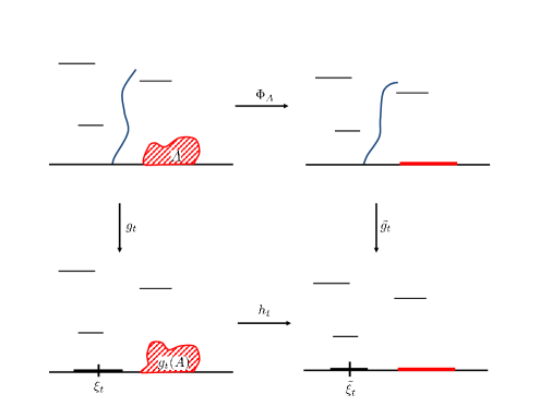
Figure 3: Conformal mappings $\Phi_{A}$ and $h_{t}$

The union of the slits in domains $\widetilde{D}$ and $\widetilde{D}_{s}$ are denoted by $\widetilde{K}=\bigcup_{j=1}^{N}\widetilde{C}_{j}$ and $\widetilde{K}(s)=\bigcup_{j=1}^{N}\widetilde{C}_{j}(s)$, respectively. Denote by $\widetilde{A}$ the set of all limiting points of $\Phi_{A}(z)$ as $z$ approaches to $A.$

Define

$$\widetilde{\xi}(t)=h_{t}(\xi(t)).$$ (6.3)

We further denote by $\widetilde{\Psi}_{t}(z,x),\;z\in\widetilde{D}_{t},\;x\in\partial{\mathbb{H}},$ the BMD-complex Poisson kernel of $\widetilde{D}_{t}.$

In this subsection, we aim at proving Proposition 6.6 for $\{\widetilde{F}_{t}\}$ stated below that is analogous to Proposition 5.13 formulated for $\{F_{t}\}.$ To this end, we prepare three lemmas and a proposition.

Lemma 6.2

$\{\widetilde{F}_{t}\}$ is strictly increasing in $t.$ It is right continuous at $t$ with limit $\widetilde{\xi}(t)$ in the following sense:

$$\bigcap_{\delta>0}\overline{\widetilde{g}_{t}(\widetilde{F}_{t+\delta}\setminus\widetilde{F}_{t})}=\{\widetilde{\xi}(t)\}.$$ (6.4)

Proof.   The first statement follows from the corresponding statement in Theorem 5.8. The second one follows from (5.24), (6.1) and (6.2) as

$$\bigcap_{t>s}\overline{\widetilde{g}_{s}(\widetilde{F}_{t}\setminus\widetilde{F}_{s})}=\bigcap_{t>s}\overline{h_{s}g_{s}\Phi_{A}^{-1}(\widetilde{F}_{t}\setminus\widetilde{F}_{s})}=\bigcap_{t>s}\overline{h_{s}g_{s}(F_{t}\setminus F_{s})}=h_{s}(\xi(s))=\widetilde{\xi}(s).$$

$\Box$

For $0\leq s<t<\tau_{A}$, set $\widetilde{g}_{t,s}=\widetilde{g}_{s}\circ\widetilde{g}_{t}^{-1}$. Denote by $\widetilde{\ell}_{t,s}$ the set of all limiting points of $\widetilde{g}_{t,s}^{-1}\circ\widetilde{g}_{s}(\widetilde{z})=g_{t}(\widetilde{z})$ as $\widetilde{z}$ approaches to $\widetilde{F}_{t}\setminus\widetilde{F}_{s}.$

Lemma 6.3

(i) $\widetilde{\ell}_{t,s}$ is a compact subset of $\partial{\mathbb{H}}$ and

$$\widetilde{a}_{t}-\widetilde{a}_{s}=\frac{1}{\pi}\int_{\widetilde{\ell}_{t,s}}\Im\widetilde{g}_{t,s}(x+i0+)dx,$$ (6.5)

$$\widetilde{g}_{s}(z)-\widetilde{g}_{t}(z)=\int_{\widetilde{\ell}_{t,s}}\widetilde{\Psi}_{t}(\widetilde{g}_{t}(z),x)\Im\widetilde{g}_{t,s}(x+i0+)dx,\quad z\in\widetilde{D}\cup\partial_{p}\widetilde{K}\setminus\widetilde{F}_{t},$$ (6.6)

where $\Im\widetilde{g}_{t,s}(x+i0)$ is the Fatou boundary limit existing a.e. on $\widetilde{\ell}_{t,s}.$

(ii) $\widetilde{a}_{t}>0$ and $\widetilde{a}_{t}$ is strictly increasing.

(iii) For each $t>0$ and $z\in\widetilde{D}\setminus\widetilde{F}_{t},$ $\sup_{0\leq s\leq t}|\widetilde{g}_{s}(z)|<\infty.$

Proof.  (i)  This can be shown in the same way as that for Lemma 5.14. The identity (6.6) can be obtained first for $z\in\widetilde{D}\setminus\widetilde{F}_{t}$ and then extended to $z\in\widetilde{D}\cup\partial_{p}\widetilde{K}\setminus\widetilde{F}_{t}.$

(ii) This can be proved exactly in the same way as that for Lemma 5.15 (iii) by the probabilistic expression (7.20) for $\widetilde{a}_{t}.$

(iii)  For $0\leq s\leq t$, (6.5) and (6.6) imply that $\displaystyle|\widetilde{g}_{s}(z)|\leq|\widetilde{g}_{t}(z)|+\pi\sup_{x\in\widetilde{\ell}_{t,0}}|\widetilde{\Psi}_{t}(\widetilde{g}_{t}(z),x)|\,\widetilde{a}_{t}.$ $\Box$

We next present a probabilistic representation of $\Im\widetilde{g}_{t}(z)$ which enables us to derive the joint continuity of $\Im\widetilde{g}_{t}(z)$ with a uniform bound from those of $\Im g_{t}(z)$.

For $D={\mathbb{H}}\setminus\bigcup_{j=1}^{N}C_{j}$, we consider Jordan curves $\eta_{j}$ surrounding $C_{j}$ that are mutually disjoint and disjoint from $F_{t}\cup A\cup\partial{\mathbb{H}}.$ Denote by $Z^{D,*}=(Z_{\cdot}^{D,*},{\mathbb{P}}_{z}^{D,*})$ the BMD on $D\cup\{c_{1}^{*},\cdots,c_{N}^{*}\}$ obtained from the absorbing Brownian motion (ABM) $Z^{\mathbb{H}}=(Z_{\cdot}^{\mathbb{H}},{\mathbb{P}}_{z}^{\mathbb{H}})$ on ${\mathbb{H}}$ by rendering each slit $C_{j}$ into a single point $c_{j}^{*}$, and set $K=\bigcup_{j=1}^{N}C_{j}$. Notice that $Z^{D,*}$ was denoted as $Z^{{\mathbb{H}},*}$ in [CFR]. The notation $Z^{D,*}$ is more convenient for later discussions. Define a measure $\nu_{j}$ on $\eta_{j}$ by

$$\nu_{j}(B)={\mathbb{P}}_{c_{j}^{*}}^{D,*}(Z_{\sigma_{\eta_{j}}}^{D,*}\in\Gamma),\quad\Gamma\in{\cal B}(\eta_{j}),\quad 1\leq j\leq N.$$ (6.7)

Proposition 6.4

(i) Define for $z\in D\setminus(F_{t}\cup A)$,

$$q_{t}(z)=\Im g_{t}(z)-\sum_{j=1}^{N}\kappa_{j}(t)\;{\mathbb{P}}_{z}^{\mathbb{H}}\left(Z_{\sigma_{K}}^{\mathbb{H}}\in C_{j};\;\sigma_{K}<\sigma_{A}\right)-{\mathbb{E}}_{z}^{\mathbb{H}}\left[\Im g_{t}(Z_{\sigma_{A}}^{\mathbb{H}});\;\sigma_{A}<\sigma_{K}\right],$$ (6.8)

where $\kappa_{j}(t)$ is the $y$-coordinate of the $j$th slit of $D_{t}.$ It holds for $z\in\widetilde{D}\setminus\widetilde{F}_{t}$ that

$$\Im\widetilde{g}_{t}(z)=q_{t}(\Phi_{A}^{-1}z)+\sum_{i=1}^{N}{\mathbb{P}}_{\Phi_{A}^{-1}z}^{\mathbb{H}}\left(Z_{\sigma_{K}}^{\mathbb{H}}\in C_{i};\;\sigma_{K}<\sigma_{A}\right)\;\sum_{j=1}^{N}\gamma_{ij}\int_{\eta_{j}}\;q_{t}(z)\nu_{j}(dz),$$ (6.9)

for some positive constants $\gamma_{ij}$, $1\leq i,j\leq N$, independent of $t$.

(ii)  For each $T\in(0,\tau_{A}),$ the function $\Im\widetilde{g}_{t}(z)$ is extended to be jointly continuous in $(t,z)\in[0,T]\times\overline{\mathbb{H}}\setminus\overline{\widetilde{F}_{T}}\setminus\overline{\widetilde{A}}$ and has a bound, for some constant $\gamma>0,$

$$0\leq\Im\widetilde{g}_{t}(z)\leq\Im\Phi_{A}^{-1}z+\gamma\quad{\rm for}\quad t\in[0,T],\ z\in\overline{\mathbb{H}}\setminus\overline{\widetilde{F}_{T}}\setminus\overline{\widetilde{A}}.$$ (6.10)

Proof. (i)  For $D_{t}={\mathbb{H}}\setminus K(t),\ K(t)=\bigcup_{j=1}^{N}C_{j}(t),$ $g_{t}(\eta_{j})$ are Jordan curves surrounding $C_{j}(t)$ that are mutually disjoint and disjoint from $g_{t}(A)\cup\partial{\mathbb{H}}.$ Let $Z^{D_{t},*}=(Z_{\cdot}^{D_{t},*},{\mathbb{P}}_{z}^{D_{t},*})$ be the BMD on $D_{t}\cup\{c_{1}^{*}(t),\cdots,c_{N}^{*}(t)\}$ obtained from the ABM $Z^{\mathbb{H}}=(Z_{\cdot}^{\mathbb{H}},{\mathbb{P}}_{z}^{\mathbb{H}})$ on ${\mathbb{H}}$ by rendering each slit $C_{j}(t)$ into a single point $c_{j}^{*}(t)$. Analogously to (6.7), define a measure $\nu_{j}^{t}$ on $g_{t}(\eta_{j})$ by

$$\nu_{j}^{t}(\Gamma)={\mathbb{P}}_{c_{j}^{*}(t)}^{D_{t},*}\left(Z_{\sigma_{g_{t}(\eta_{j})}}^{D_{t},*}\in\Gamma\right),\quad\Gamma\in{\cal B}(g_{t}(\eta_{j})),\quad 1\leq j\leq N.$$ (6.11)

Owing to the conformal invariance of the BMD (see [CF1, Remark 7.8.2]), we have

$$\nu_{j}^{t}(g_{t}(\Gamma))=\nu_{j}(\Gamma)\quad\hbox{for any }\Gamma\in{\cal B}(\eta_{j}).$$ (6.12)

Applying [CFR, Theorem 7.1] to the canonical map $h_{t}$ from $D_{t}\setminus g_{t}(A)$ with $g_{t}(\eta_{j})$ in place of $\eta_{j},\ 1\leq j\leq N$, we get

$$\begin{cases}\Im h_{t}(z)=v_{t}(z)+\sum_{j=1}^{N}f_{j}(t,z)v_{t}^{*}(c_{j}^{*}(t))\\ v_{t}(z)=\Im z-{\mathbb{E}}_{z}^{\mathbb{H}}\left[\Im Z_{\sigma_{K_{t}\cup g_{t}(A)}}^{\mathbb{H}};\sigma_{K_{t}\cup g_{t}(A)}<\infty\right]\\ v_{t}^{*}(c_{j}^{*}(t))=\sum_{k=1}^{N}\frac{M_{jk}(t)}{1-R_{k}^{*}(t)}\int_{g_{t}(\eta_{k})}v_{t}(z)\nu_{k}^{t}(dz).\end{cases}$$ (6.13)

Here

$$f_{j}(t,z)={\mathbb{P}}_{z}^{\mathbb{H}}\left(Z_{\sigma_{K_{t}}}^{\mathbb{H}}\in C_{j}(t);\sigma_{K_{t}}<\sigma_{g_{t}(A)}\right),\quad R_{k}^{*}(t)=\int_{g_{t}(\eta_{k})}f_{k}(t,z)\nu^{t}_{j}(dz),$$ (6.14)

and $M_{jk}(t)$ is the entry of $\sum_{n=0}^{\infty}Q^{*}(t)^{n}$ for the matrix $Q^{*}(t)$ with zero diagonal entry and off-diagonal entry given by

$$q_{ij}^{*}(t)={\mathbb{P}}_{c_{i}^{*}(t)}^{D_{t},*}(Z_{\sigma_{K^{*}(t)}}^{D_{t},*}=c_{j}^{*}(t),\;\sigma_{K^{*}(t)}<\sigma_{g_{t}(A)})/(1-R_{i}^{*}(t)),\ i\neq j.$$ (6.15)

By the conformal invariance of the ABM $Z^{\mathbb{H}}$ under the map $g_{t}$ (see [CF1, Theorem 5.3.1]),

$$f_{j}(t,g_{t}(z))={\mathbb{P}}_{z}^{\mathbb{H}}\left(Z_{\sigma_{K}}^{\mathbb{H}}\in C_{j},\;\sigma_{K}<\sigma_{A}\right)$$ (6.16)

and

$$v_{t}(g_{t}(z))=\Im g_{t}(z)-{\mathbb{E}}_{z}^{\mathbb{H}}\left[\Im g_{t}(Z_{\sigma_{K\cup A}}^{\mathbb{H}});\;\sigma_{K\cup A}<\infty\right]=:q_{t}(z).$$ (6.17)

Thus by (6.12),

$$\begin{cases}R_{k}^{*}(t)=\int_{\eta_{k}}{\mathbb{P}}_{z}^{\mathbb{H}}(Z_{\sigma_{K}}^{\mathbb{H}}\in C_{k};\sigma_{K}<\sigma_{A})\nu_{k}(dz)=:R_{k}^{*},\\ \int_{g_{t}(\eta_{k})}v_{t}(z)\nu_{k}^{t}(dz)=\int_{\eta_{k}}q_{t}(z)\nu_{k}(dz).\end{cases}$$ (6.18)

Finally we use again the conformal invariance of the BMD $Z^{D,*}$ under the map $g_{t}$ to get from (6.15)

$$q_{ij}^{*}(t)={\mathbb{P}}_{c_{i}^{*}}^{D,*}(Z_{\sigma_{K^{*}}}^{D,*}=c_{j}^{*},\;\sigma_{K^{*}}<\sigma_{A})/(1-R_{i}^{*})=:q_{ij}^{*},\ i\neq j.$$ (6.19)

Denote by $M_{ij}$ is the entry of $\sum_{n=0}^{\infty}(Q^{*})^{n}$ for the matrix $Q^{*}$ with zero diagonal entry and off-diagonal entry $q_{ij}^{*}.$ It follows from (6.13) and (6.16)-(6.19) that

$$\Im h_{t}\circ g_{t}(z)=q_{t}(z)+\sum_{i=1}^{N}{\mathbb{P}}_{z}^{\mathbb{H}}\left(Z_{\sigma_{K}}^{\mathbb{H}}\in C_{i};\;\sigma_{K}<\sigma_{A}\right)\;\sum_{j=1}^{N}\gamma_{ij}\int_{\eta_{j}}\;q_{t}(z)\nu_{j}(dz),$$ (6.20)

for $z\in D\setminus F_{t}\setminus A,$ where $\gamma_{ij}=\frac{M_{ij}}{1-R_{j}^{*}}.$ This together with (6.2) establishes (6.9).

(ii) As $g_{t}(z)$ is a solution of the K-L equation (5.19), $\Im g_{t}(z)$ is jointly continuous and satisfies $0\leq\Im g_{t}(z)\leq\Im z.$ The functions $\{\kappa_{j}(t);1\leq j\leq N\}$ are continuous due to the continuity of ${\bf s}(t).$ Therefore by (6.8), $q_{t}(z)$ is jointly continuous. Since the function $u(z)=\Im z$ is excessive with respect to $Z^{\mathbb{H}}$, $v_{t}(z)$ defined by (6.13) is non-negative. Hence $0\leq q_{t}(z)=v_{t}(g_{t}(z))\leq\Im g_{t}(z)\leq\Im z$. It follows from (6.9) that $\Im\widetilde{g}_{t}(z)$ is jointly continuous in $(t,z)\in[0,T]\times(\widetilde{D}\setminus\widetilde{F}_{T})$ and $q_{t}(\Phi_{A}^{-1}z)\leq\Im\Phi_{A}^{-1}z$. Thus we readily obtain the stated joint continuity with a bound (6.10). $\Box$

Lemma 6.5

(i)  For each $T\in(0,\tau_{A})$, the functions $\{\widetilde{g}_{t}(z),t\in[0,T]\}$ are extended to be locally equi-continuous and locally uniformly bounded in $z\in(\widetilde{D}\cup\partial_{p}\widetilde{K}\cup\partial{\mathbb{H}})\setminus\overline{\widetilde{F}_{T}}\setminus\overline{\widetilde{A}}.$

(ii) For $s\geq 0,$ $\lim_{t\downarrow s}\widetilde{g}_{t,s}^{-1}(z)=z$ uniformly on each compact subset of $\widetilde{D}_{s}\cup\partial_{p}\widetilde{K}(s)\cup(\partial{\mathbb{H}}\setminus\{\widetilde{\xi}(s)\}\setminus\widetilde{g}_{s}(\widetilde{A})).$

(iii)  For $T\in[0,\tau_{A}),$ $\widetilde{g}_{t}(\widetilde{z})$ is jointly continuous in $(t,\widetilde{z})\in[0,T]\times[(\widetilde{D}\cup\partial_{p}\widetilde{K}\cup\partial{\mathbb{H}})\setminus\overline{\widetilde{F}_{T}}\setminus\widetilde{A}].$

(iv) $\widetilde{a}_{t}$ is right continuous in $t$ and $\widetilde{D}_{t}$ is continuous in $t$.

(v)  $\widetilde{\Psi}_{t}(z,x)$ is jointly continuous in $(t,z,x)\in\bigcup_{t\in[0,\tau_{A})}\{t\}\times[\widetilde{D}_{t}\cup\partial_{p}\widetilde{K}(t)\cup(\partial{\mathbb{H}}\setminus\{x\})]\times\partial{\mathbb{H}}$.

Proof.  (i) follows from Proposition 6.4 (ii) together with Lemma 6.3 (iii) exactly in the same way as the proof of [CFR, Theorem 7.4]. (ii) follows from (i) and Proposition 6.4 (ii) as the proof of [CFR, Theorem 8.2]. (iii) can be shown in a quite similar way to (ii). The right continuity of $\widetilde{a}_{t}$ follows from (ii) as the proof of [CFR, Theorem 8.4]. The continuity of $\widetilde{D}_{t}$ is a consequence of (iii). (v) follows from the continuity of $\widetilde{D}_{t}$ in (iv) and the Lipschitz continuity of $\widetilde{\Psi}$ as the proof of [CFR, Theorem 9.8]. $\Box$

Proposition 6.6

$\widetilde{a}_{0}=0,$ $\widetilde{a}_{t}$ is strictly increasing and right continuous. For each $T\in(0,\tau_{A})$ and $z\in\widetilde{D}\cup\partial_{p}\widetilde{K}\setminus\widetilde{F}_{T},$ $\widetilde{g}_{t}(z)$ is right differentiable in $\widetilde{a}_{t}$ and

$$\frac{\partial^{+}\widetilde{g}_{t}(z)}{\partial\widetilde{a}_{t}}=-\pi\widetilde{\Psi}_{t}(\widetilde{g}_{t}(z),\widetilde{\xi}(t)),\quad\widetilde{g}_{0}(z)=z,\quad{\rm for}\quad t\in[0,T].$$ (6.21)

Here the left hand side indicates the right derivative.

Proof.  This follows from Lemma 6.2, Lemma 6.3 and Lemma 6.5 just as in the proof of Proposition 5.13. $\Box$

Note that equation (6.21) does not characterize the conformal map $\widetilde{g}_{t}$ since its left hand side involves only the right derivative. To characterize $\widetilde{g}_{t}$ uniquely, we need to show that $\widetilde{g}_{t}$ is differentiable in $t$; see [CFS, Remark 2.7]. The first assertion of the next proposition is crucial not only for this purpose but also in legitimating the stochastic calculus in the next subsection.

The conformal map $h_{t}(z)$ (resp. $\Phi_{A}(z)$) from $D_{t}\setminus g_{t}(A)$ (resp. $D\setminus A$) onto $\widetilde{D}_{t}$ (resp. $\widetilde{D}$) is extended to a conformal map on

$$\left(D_{t}\cup\Pi D_{t}\cup\partial{\mathbb{H}}\right)\setminus\left(g_{t}(\overline{A})\cup\Pi g_{t}(A)\right)\quad{\rm(resp.}\left(D\cup\Pi D\cup\partial{\mathbb{H}}\right)\setminus\left(\overline{A}\cup\Pi A\right){\rm)}$$ (6.22)

by the Schwarz reflection. Note that $h_{0}(z)=\Phi_{A}(z)$.

Proposition 6.7

(i) For any $t\in(0,\tau_{A})$ and $z\in D_{t}\cup\partial{\mathbb{H}}\setminus\overline{g_{t}(A)},$ $h_{t}(z),\;h_{t}^{\prime}(z),\;h_{t}^{\prime\prime}(z)$ are jointly continuous in $(t,z)$.

(ii) Locally uniformly in $z\in(D\cup\partial{\mathbb{H}})\setminus\overline{A},$

$$\lim_{t\downarrow 0}h_{t}(z)=\Phi_{A}(z),\quad\lim_{t\downarrow 0}h_{t}^{\prime}(z)=\Phi_{A}^{\prime}(z),\quad\lim_{t\downarrow 0}h_{t}^{\prime\prime}(z)=\Phi_{A}^{\prime\prime}(z).$$ (6.23)

Proof.  (i) It follows from (6.2) that for $t\in[0,\tau_{A}),\ 0\leq s<t$ and $z\in D_{t}\setminus g_{t}(A),$

$$h_{t}(z)=\widetilde{g}_{t,s}^{-1}\circ h_{s}\circ g_{t,s}(z)\quad\hbox{ where }\ g_{t,s}=g_{s}\circ g_{t}^{-1}\hbox{ and }\ \widetilde{g}_{t,s}=\widetilde{g}_{s}\circ\widetilde{g}_{t}^{-1}.$$ (6.24)

For $t>0$ and $z\in D_{t}\cup(\partial{\mathbb{H}}\setminus\{\xi(t)\}),$ let $\varphi(u;t,z),\ u\in I_{t,z},$ be the unique solution of the ODE (5.1) in variable $u$ with initial condition $\varphi(t;t,z)=z$ and with the maximal time interval $I_{t,z}$ of existence. If $z\in D_{t},$ then $I_{t,z}=[0,t_{z})$ by Proposition 5.4 and it holds that $\varphi(u;t,z)=g_{t,u}(z)$ for $u\in[0,t].$ But, if $z\in\partial{\mathbb{H}}\setminus\{\xi(t)\},$ then $\varphi(\cdot;t,z)$ is a continuous motion on $\partial{\mathbb{H}}$ and it could be that $I_{t,z}=(\alpha_{t,z},\beta_{t,z})$ with $0\leq\alpha_{t,z}<t<\beta_{t,z}$. Our strategy for the proof of (i) is to use the identity (6.24) for some fixed $s\in(0,t)$ along with the joint continuity of $\varphi(s;t,z)$ and that of $\widetilde{g}_{t,s}^{-1}(\widetilde{z})=\widetilde{g}_{t}\circ\widetilde{g}_{s}^{-1}(\widetilde{z})$ basically shown in Lemma 6.5.

Recall that $\tau_{A}=\inf\{u>0:\overline{F}_{u}\cap\overline{A}\neq\emptyset\})$ and define $\Pi z=\bar{z},\;z\in{\mathbb{H}}.$. Fix $T\in(0,\tau_{A})$. Take any smooth Jordan curve $\Gamma\subset{\mathbb{C}}$ with $\Pi\Gamma=\Gamma$ such that $\Gamma$ surrounds $\overline{F}_{T},$ the sets $\overline{A}$ and $K=\cup_{j=1}^{N}C_{j}$ are located outside $\Gamma,$ and $\Gamma$ intersects $\partial{\mathbb{H}}$ at only two points. For $t\in(0,T),$ we extend $g_{t}$ by the Schwarz reflection and let $\Gamma_{t}=g_{t}(\Gamma).$ Then $\Gamma_{t}$ surrounds $\overline{g_{t}(F_{T}\setminus F_{t})}$ and the sets $\overline{g_{t}(A)}$ and $K(t)$ are located outside $\Gamma_{t}.$ In particular, $\xi(t)\notin\Gamma_{t}$ in view of (5.24).

From now we fix an arbitrary $t\in(0,T)$ and let $\Gamma_{t}\cap\partial{\mathbb{H}}=\{z_{1},z_{2}\}.$ The ODE (5.1) and its solution $\varphi(u;t,z),u\in I_{t,z},$ are extended to $\Pi D_{t}$ by mirror reflection. We then choose any $s\in(\alpha_{t,z_{1}}\vee\alpha_{t,z_{2}},t)$ so that $\varphi(s;t,z)$ is well defined for all $z\in\Gamma_{t}.$ According to a general theorem [H, Theorem V.2.1] on ODE, $(t,z)\mapsto\varphi(s;t,z)$ is joint continuous in the following sense:  for any $\varepsilon>0,$ there exists $\delta=\delta(\varepsilon,t,z)>0$ with $s<t-\delta<t+\delta<T$ such that, for any $u>0,\ w\in{\mathbb{C}}$ with $|u-t|<\delta,\ |w-z|<\delta,$ we have $\alpha_{u,w}<s$ and $|\varphi(s;u,w)-\varphi(s;t,z)|<\varepsilon$ for any $z\in\Gamma_{t}.$ A covering argument then yields the existence of $\delta\in(0,t-s)$ such that

$$\alpha_{u,z}<s\ {\rm and}\ |\varphi(s;u,z)-\varphi(s;t,z)|<\varepsilon\ \text{\rm for any}\ u\in[t-\delta,t+\delta]\ \text{\rm and for any}\ z\in\Gamma_{t}.$$ (6.25)

Observe that $\varphi(s;t,z)=g_{t,s}(z)$ for $z\in D_{t}.$ Hence, by the continuity of $\varphi(s;t,z)$ in $z$, we get the identity $\{w=\varphi(s;t,z):z\in\Gamma_{t}\}=\Gamma_{s}.$ We can choose $\varepsilon>0$ so that the $\varepsilon-$neighborhood $\Gamma_{s,\varepsilon}$ of $\Gamma_{s}$ is disjoint from $\overline{g_{s}(F_{T}\setminus F_{s})}\cup\overline{g_{s}(A)}.$ On account of the relation $h_{s}(w)=\widetilde{g}_{s}\circ\Phi_{A}\circ g_{s}^{-1}(w),\ w\in D_{s},$ we have

$$h_{s}(\Gamma_{s,\varepsilon})\subset\widetilde{D}_{s}\cup\Pi\widetilde{D}_{s}\cup\partial{\mathbb{H}}\setminus\left(\overline{\widetilde{g}_{s}(\widetilde{F}_{T}\setminus\widetilde{F}_{s})}\cup\widetilde{\Pi}\widetilde{g}_{s}(\widetilde{F}_{T}\setminus\widetilde{F}_{s}))\cup\widetilde{g}_{s}(\widetilde{A})\cup\Pi\widetilde{g}_{s}(\widetilde{A})\right).$$ (6.26)

On the other hand, we have the following variant of Lemma 6.5 (iii):

$${\rm For}\ T\in(0,\tau_{A})\ {\rm and}\ s\in[0,T),\ \widetilde{g}_{u,s}^{-1}(\widetilde{z})=\widetilde{g}_{u}(\widetilde{g}_{s}^{-1}(\widetilde{z}))\ \text{\rm is jointly continuous in}$$

$$(u,\widetilde{z})\in[s,T]\times[(\widetilde{D}_{s}\cup\partial{\mathbb{H}})\setminus\overline{\widetilde{g}_{s}(\widetilde{F}_{T}\setminus\widetilde{F}_{s})}\setminus\widetilde{g}_{s}(\widetilde{A})].$$ (6.27)

This can be proved as follows. By using the relation (6.24), we first express $\Im\widetilde{g}_{u,s}^{-1}$, $u\geq s$, in terms of the BMD on $\widetilde{D}_{s}$ and the ABM on ${\mathbb{H}}$ in analogy to (6.9), which yields the joint continuity of $\Im\widetilde{g}_{u,s}^{-1}(\widetilde{z})$ in $(u,\widetilde{z})\in[s,T]\times[\overline{\mathbb{H}}\setminus\overline{\widetilde{g}_{s}(\widetilde{F}_{T}\setminus\widetilde{F}_{s})}\setminus\widetilde{g}_{s}(\widetilde{A})].$ This combined with Lemma 6.3 (iii) (replacing $(s,t)$ by $(u,T)$) implies, in the same way as the proof of [CFR, Theorem 7.4], the local uniform boundedness of the family $\{\widetilde{g}_{u,s}^{-1}(\widetilde{z});u\in[s,T]\}$ in $\widetilde{z}\in\widetilde{D}_{s}\cup\partial{\mathbb{H}}\setminus\overline{\widetilde{g}_{s}(\widetilde{F}_{T}\setminus\widetilde{F}_{s})}\setminus\widetilde{g}_{s}(\widetilde{A})].$ Thus we can get (6.2) as the proof of [CFR, Theorem 8.2].

By [H, Theorem V.2.1] again, $\varphi(s;u,z)$ is jointly continuous in $(u,z)\in[t-\delta,t+\delta]\times\Gamma_{t}.$ Since $h_{s}(\varphi(s;u,z))\in h_{s}(\Gamma_{s,\varepsilon})$ by (6.25), we conclude from (6.26) and (6.2) that the relation (6.24) extends to $h_{u}(z)=\widetilde{g}_{u,s}^{-1}(h_{s}(\varphi(s;u,z))$ to be jointly continuous at each $(u,z)\in[t-\delta,t+\delta]\times\Gamma_{t}.$ In particular $\sup_{u\in[t-\delta,t+\delta],\;z\in\Gamma_{t}}|h_{u}(z)|$ is finite. Moreover, by the joint continuity of the solution of (5.1), we may assume that $\Gamma_{t}\subset\bigcap_{u\in[t-\delta,t+\delta]}(D_{u}\setminus\overline{g_{u}(A)})$.

As $h_{u}$ is analytic, the Cauchy integral formula yields that $h_{u}(z),\;h_{u}^{\prime}(z),\;h_{u}^{\prime\prime}(z)$ are jointly continuous in $(u,z)\in[t-\delta,t+\delta]\times U(t)$, where $U(t)$ is an open set enclosed by $\Gamma_{t}.$

(ii) We continue to work with the function $\varphi(u;t,z),\ u\in I_{t,z},$ as above and claim the following: for any $\varepsilon>0,$ there exists $\delta>0$ such that, for any $t\in(0,\delta]$ and any $z\in\partial{\mathbb{H}}\setminus[\xi(0)-\varepsilon,\xi(0)+\varepsilon],$ $I_{t,z}=[0,\beta)$ for some $\beta>t.$

To see this, we fix $\varepsilon_{1}\in(0,\varepsilon)$ and take $t_{0}>0$ with $\{\xi(u):u\in[0,t_{0}]\}\subset(\xi(0)-\varepsilon_{1},\xi(0)+\varepsilon_{1}).$ Since the solution $\varphi(t,u,\xi(0)\pm\varepsilon_{1})$ of (5.1) with $\varphi(u,u,\xi(0)\pm\varepsilon_{1})=\xi(0)\pm\varepsilon_{1}$ is jointly continuous in $(t,u),$ there is $\delta\in(0,t_{0}]$ with $\xi(0)-\varepsilon<\inf_{0\leq u\leq t\leq\delta}\varphi(t,u,\xi(0)-\varepsilon_{1}),\ \sup_{0\leq u\leq t\leq\delta}\varphi(t,u,\xi(0)+\varepsilon_{1})<\xi(0)+\varepsilon.$ Take any $t\in(0,\delta]$ and any $z\in\partial{\mathbb{H}}$ with $z>\xi(0)+\varepsilon.$ Suppose $I_{t,z}=(\alpha,\beta)$ for some $\alpha\in(0,t).$ As $\liminf_{u\downarrow\alpha}|\varphi(u,t,z)-\xi(u)|=0,$ we find $u_{1}\in(\alpha,t)$ with $\varphi(u_{1},t,z)=\xi(0)+\varepsilon_{1},$ arriving at a contradiction $z=\varphi(t,u_{1},\xi(0)+\varepsilon_{1})<\xi(0)+\varepsilon$. Hence $I_{t,z}=[0,\beta).$ The same is true for $z\in\partial{\mathbb{H}}$ with $z<\xi(0)-\varepsilon.$

Observe that $g_{t}^{-1}(z)=\varphi(0,t,z)$ for $(t,z)\in[0,\delta]\times(D\cup[(\partial{\mathbb{H}}\setminus[\xi(0)-\varepsilon,\xi(0)+\varepsilon])],$ and it is jointly continuous in $(t,z)$ there by the theorem cited above. Let $V$ be a compact subset of $D\cup(\partial{\mathbb{H}}\setminus[\xi(0)-\varepsilon,\xi(0)+\varepsilon])\setminus\overline{A}.$ We may assume that $\delta<\tau_{A}$ and $V$ is disjoint from $\bigcup_{s\in[0,\delta]}\overline{g_{s}(A)}.$

Combining this with the identity $h_{t}=\widetilde{g}_{t}\circ\Phi_{A}\circ g_{t}^{-1}$ from (6.2) and with Lemma 6.5 (ii), (iii), we see that $h_{t}(z)$ is jointly continuous at each $(t,z)\in[0,\delta]\times V$ and consequently $\sup_{t\in[0,\delta]\;z\in V}|h_{t}(z)|$ is finite and $\lim_{t\downarrow 0}h_{t}(z)=\Phi_{A}(z)$ for each $z\in V.$ By taking appropriate circles as $V$, we get the local uniform convergence (6.23) in a similar way as in the proof of (i). $\Box$

In the remaining part of this paper, the derivative of a function $f$ in the time parameter will be designated by $\dot{f}$.

Theorem 6.8

For $s\in(0,\tau_{A})$ and $z\in\widetilde{D}\cup\partial_{p}\widetilde{K}\cup\widetilde{F}_{t}$, $\widetilde{g}_{s}(z)$ is continuously differentiable in $s\in[0.t]$ and

$$\frac{d\widetilde{g}_{s}(z)}{ds}=-2\pi|h_{s}^{\prime}(\xi(s))|^{2}\;\widetilde{\Psi}_{s}(\widetilde{g}_{s}(z),\widetilde{\xi}(s)),\quad g_{0}(z)=z.$$ (6.28)

Proof.  It suffices to prove

$$\dot{\widetilde{a}_{s}}\;=\;2|h_{s}^{\prime}(\xi(s))|^{2}.$$ (6.29)

This is because (6.29) together with (6.21) implies that (6.28) holds with the right derivative $\frac{\partial^{+}\widetilde{g}_{s}(z)}{ds}$ in place of $\frac{\partial\widetilde{g}_{s}(z)}{ds}$. But since the right hand side of (6.28) is continuous in $s$ in view of Lemma 6.5 and Proposition 6.7, $\widetilde{g}_{s}(\widetilde{z})$ is actually continuously differentiable in $s$.

For $D\in{\cal D}$ and an ${\mathbb{H}}$-hull $K\subset D,$ we denote by ${\rm Cap}^{D}(K)$ (resp. ${\rm Cap}^{\mathbb{H}}(K)$) the half-plane capacity of $K$ for the canonical map from $D\setminus K$ (resp. the Riemann map from ${\mathbb{H}}\setminus K$ onto ${\mathbb{H}}$). For a set $A\subset{\mathbb{H}}$, we put ${\rm rad}(A)=\sup_{z\in A}|z|.$ Fix $s\geq 0$ and let $K_{\epsilon}=g_{s}(F_{s+\epsilon}\setminus F_{s})$ and $\widetilde{K}_{\epsilon}=\widetilde{g}_{s}(\widetilde{F}_{s+\epsilon}\setminus\widetilde{F}_{s})$. Then ${\rm rad}(K_{\epsilon}\setminus\{\xi(s)\})=o(\epsilon)$ and ${\rm rad}(\widetilde{K}_{\epsilon}\setminus\{\widetilde{\xi}(s)\})=o(\epsilon)$ by (5.24) and (6.4), respectively. Consequently we have by Theorem 7.1 of Appendix

$${\rm Cap}^{D_{s}}(K_{\epsilon})-{\rm Cap}^{\mathbb{H}}(K_{\epsilon})=o(\epsilon),\quad{\rm Cap}^{\widetilde{D}_{s}}(\widetilde{K}_{\epsilon})-{\rm Cap}^{\mathbb{H}}(\widetilde{K}_{\epsilon})=o(\epsilon).$$ (6.30)

Since $\widetilde{K}_{\epsilon}=h_{s}(K_{\epsilon}),$ we get from (6.30) and [L1, (4.15)] that

$$\widetilde{a}_{s+\epsilon}-\widetilde{a}_{s}={\rm Cap}^{\widetilde{D}_{s}}(\widetilde{K}_{\epsilon})={\rm Cap}^{\mathbb{H}}(h_{s}(K_{\epsilon}))+o(\epsilon)$$

$$=\Phi^{\prime}_{s}(\xi(s))^{2}{\rm Cap}^{\mathbb{H}}(K_{\epsilon})+o(\epsilon)=\Phi^{\prime}_{s}(\xi(s))^{2}{\rm Cap}^{D_{s}}(K_{\epsilon})+o(\epsilon)=\Phi^{\prime}_{s}(\xi(s))^{2}(a_{s+\epsilon}-a_{s})+o(\epsilon),$$

which yields (6.29) as $a_{s+\epsilon}-a_{s}=2\epsilon$ by Theorem 5.12. $\Box$

6.3 Characterization of locality of ${\rm SKLE}_{\alpha,-b_{\rm BMD}}$

We continue to operate under the setting in the preceding subsection. To investigate the locality, we need to compute the driving processes for $\{\widetilde{F}_{t};t<\tau_{A}\}$. It follows from (5.19) that the inverse map $g_{t}^{-1}$ of $g_{t}$ satisfies

$$\dot{g}_{t}^{-1}(z)=2\pi(g_{t}^{-1})^{\prime}(z)\Psi_{{\bf s}(t)}(z,\xi(t)),\quad g_{0}^{-1}(z)=z.$$ (6.31)

From (6.2), we have

$$\dot{h}_{t}(z)=\dot{\widetilde{g}}_{t}(\Phi_{A}\circ g_{t}^{-1}(z))+(\widetilde{g}_{t}\circ\Phi_{A})^{\prime}(g_{t}^{-1}(z))\dot{g}_{t}^{-1}(z),\quad z\in D_{t}\setminus g_{t}(A).$$

This together with (6.31), Theorem 6.8, and then by (6.2) again yields that for $z\in D_{t}\setminus g_{t}(A)$,

$$\dot{h}_{t}(z) = -2\pi|h_{t}^{\prime}(\xi(t))|^{2}\widetilde{\Psi}_{t}(\widetilde{g}_{t}\circ\Phi_{A}\circ g_{t}^{-1}(z),\widetilde{\xi}(t))+(\widetilde{g}_{t}\circ\Phi_{A})^{\prime}(g_{t}^{-1}(z))2\pi(g_{t}^{-1})^{\prime}(z)\Psi_{{\bf s}(t)}(z,\xi(t))$$ (6.32)

$$= -2\pi|h_{t}^{\prime}(\xi(t))|^{2}\widetilde{\Psi}_{t}(h_{t}(z),h_{t}(\xi(t)))+2\pi h_{t}^{\prime}(z)\Psi_{{\bf s}(t)}(z,\xi(t)).$$

Functions $h_{t}(z)$ and $h_{t}^{\prime}(z)$ are extended to the region (6.22), call it $G_{t}$, by the Schwarz reflection. Fix $t_{0}>0$ and take a disk $B$ centered at $\xi(t_{0})$ with $\overline{B}\subset\cap_{|t-t_{0}|\leq\delta}G_{t}$ and $\{\xi(t):|t-t_{0}|\leq\delta\}\subset B$ for some $\delta>0.$ Denote the right hand side of (6.32) by $f(t,z).$ By virtue of Proposition 6.7(i), Lemma 6.5(v) and Proposition 5.1(i), $f(t,z)$ is jointly continuous and hence uniformly bounded in $(t,z)\in[t_{0}-\delta,t_{0}+\delta]\times(\partial B\cap\overline{\mathbb{H}})$. By taking Schwarz reflections of $\widetilde{\Psi}_{t}(z,h_{t}(\xi(t)))$ and $\Psi_{{\bf s}(t)}(z,\xi(t))$ in $z$, $f(t,z)$ admits an extension to $[t_{0}-\delta,t_{0}+\delta]\times\partial B$ to be jointly continuous and uniformly bounded there, and the identity $\dot{h}_{t}(z)=f(t,z)$ extends to $(t,z)\in(t_{0}-\delta,t_{0}+\delta)\times(\partial B\setminus\partial{\mathbb{H}}).$

Expressing $(h_{u}(z)-h_{t}(z))/(u-t),\ z\in B,\;t\in(t_{0}-\delta,t_{0}+\delta),$ by the Cauchy integral formula and letting $u\to t$, we see that $h_{t}(z)$ is differentiable in $t$ for any $z\in B$ with $\dot{h}_{t}(z)$ being analytic in $z\in B$ and jointly continuous in $(t,z)\in(t_{0}-\delta,t_{0}+\delta)\times B.$ In particular, $\dot{h}_{t}(\xi(t))$ can be computed by $\lim_{z\to\xi(t),\;z\in{\mathbb{H}}}\dot{h}_{t}(z)$ explicitly. Indeed, by the definition (6.1) of $b_{\rm BMD}({\bf s},\xi)$, we get from (6.32)

$$\dot{h}_{t}(\xi(t)) = h_{t}^{\prime}(\xi(t))\,b_{\rm BMD}(\xi(t),{\bf s}(t))-|h_{t}^{\prime}(\xi(t))|^{2}\,b_{\rm BMD}(h_{t}(\xi(t)),h_{t}({\bf s}(t)))$$ (6.33)

$$+\lim_{z\to\xi(t)}\left(\frac{2|h_{t}^{\prime}(\xi(t))|^{2}}{h_{t}(z)-h_{t}(\xi(t))}-\frac{2h_{t}^{\prime}(z)}{z-\xi(t)}\right)$$

$$= h_{t}^{\prime}(\xi(t))\,b_{\rm BMD}(\xi(t),{\bf s}(t))-|h_{t}^{\prime}(\xi(t))|^{2}\,b_{\rm BMD}(h_{t}(\xi(t)),h_{t}({\bf s}(t)))-3h_{t}^{\prime\prime}(\xi(t)).$$

Thus $h_{t}(z)$ is differentiable in $t$ for each $z\in\partial{\mathbb{H}}\cap G_{t}$ with $\dot{h}_{t}(z)$ being jointly continuous in $t>0,\ z\in\partial{\mathbb{H}}\cap G_{t}.$ Moreover, $h_{t}^{\prime}(z)$ and $h_{t}^{\prime\prime}(z)$ are jointly continuous by Proposition 6.7. Since $\widetilde{\xi}(t)=h_{t}(\xi(t))$ and $\xi(t)$ is the solution of the SDE (3.32), we can readily apply a generalized Itô formula (see [CFS, Remark 2.9] and [RY, (IV.3.12)]) to get

$$d\widetilde{\xi}(t)=\left(\dot{h}_{t}(\xi(t))+h_{t}^{\prime}(\xi(t))b({\bf s}(t)-\widehat{\xi}(t))+\frac{1}{2}h_{t}^{\prime\prime}(\xi(t))\alpha({\bf s}(t)-\widehat{\xi}(t))^{2}\right)dt+h_{t}^{\prime}(\xi(t))\alpha({\bf s}(t)-\widehat{\xi}(t))dB_{t}.$$

This combined with (6.33) gives the following.

Theorem 6.9

It holds that

$$d\widetilde{\xi}(t) = h_{t}^{\prime}(\xi(t))\left(b({\bf s}(t)-\widehat{\xi}(t))+b_{\rm BMD}(\xi(t),{\bf s}(t))\right)dt+\frac{1}{2}h_{t}^{\prime\prime}(\xi(t))\left(\alpha({\bf s}(t)-\widehat{\xi}(t))^{2}-6\right)dt$$ (6.34)

$$-|h_{t}^{\prime}(\xi(t))|^{2}b_{\rm BMD}(\widetilde{\xi}(t),h_{t}({\bf s}(t)))dt+h_{t}^{\prime}(\xi(t))\alpha({\bf s}(t)-\widehat{\xi}(t))dB_{t}.$$

Let $\{\check{F}_{t}\}_{t<\check{\tau}_{A}}$ be the half-plane capacity reparametrization of the image hulls $\{\widetilde{F}_{t}\}_{t<\tau_{A}}$, namely,

$$\check{F}_{t}=\widetilde{F}_{\widetilde{a}^{-1}(2t)},\qquad\check{\tau}_{A}=\widetilde{a}(\tau_{A})/2.$$ (6.35)

where $\widetilde{a}(t)$ is the half-plane capacity of $\widetilde{F}_{t}$ and $\widetilde{a}^{-1}$ is its inverse function. Accordingly, the processes $\widetilde{\xi}(t)=h_{t}(\xi(t))=\widetilde{g}_{t}\circ\Phi_{A}(\xi)$ and $\widetilde{\bf s}_{j}(t)=h_{t}({\bf s}_{j}(t))=\widetilde{g}_{t}\circ\Phi_{A}({\bf s}_{j})$ are time-changed into

$$\check{\xi}(t)=\widetilde{\xi}(\widetilde{a}^{-1}(2t))\quad{\rm and}\quad\check{\bf s}_{j}(t)=\widetilde{\bf s}_{j}(\widetilde{a}^{-1}(2t)),\quad 1\leq j\leq 3N,\quad t<\check{\tau}_{A},$$ (6.36)

respectively.

Set $\check{g}_{t}=\widetilde{g}_{\widetilde{a}^{-1}(2t)}$ and $\check{\Psi}_{t}=\widetilde{\Psi}_{\widetilde{a}^{-1}(2t)}$. It follows from (6.28), (6.29), Lemma 6.5 (v) and Proposition 6.7(i) that, for $T\in(0,\check{\tau}_{A}),$ $\check{g}_{t}(z)$ is continuously differentiable in $t\in[0,T]$ and

$$\frac{d\check{g}_{t}(z)}{dt}=-2\pi\check{\Psi}_{t}(\check{g}_{t}(z),\check{\xi}(t)),\quad\check{g}_{0}(z)=z\in\widetilde{D}\cup\partial_{p}\widetilde{K}\setminus\check{F}_{t}.$$ (6.37)

Lemma 6.10

It holds under ${\mathbb{P}}_{(\xi,{\bf s})}$ that

$$\check{\bf s}_{j}(t)=\Phi_{A}({\bf s}_{j})+\int_{0}^{t}\check{b}_{j}(\check{\xi}(s),\check{\bf s}(s))ds,\quad t\in[0,\check{\tau}_{A}),\quad 1\leq j\leq 3N,$$ (6.38)

where $\check{b}_{j}({\bf w})=\check{b}_{j}(\xi,{\bf s})$ is defined by (3.27) with $\Psi_{s}$ being replaced by $\check{\Psi}_{s}.$

Proof.  We can get (6.38) from the K-L equation (6.37) exactly in the same way as the proof of Theorem 2.3, if Lemma 2.1 for $\check{g}_{t},\;\check{\tau}_{A},\;\check{\Psi}_{t}$ in place of $g_{t},\;t_{\gamma},\;\Psi_{t}$ is once established. Let us call Lemma 2.1’ such a counterpart of Lemma 2.1.

The first and second assertions of Lemma 2.1’ follow from Lemma 6.5 (v), Proposition 6.7(i), (6.29) and (6.37) as in the proof of those of Lemma 2.1. The third assertion of Lemma 2.1’ can be obtained by proving an analogue to (2.7) using a similar method to the proof of (6.21) combined with (6.29). The rest of assertions of Lemma 2.1’ can be proved quite similarly. $\Box$

Let $M_{t}=\int_{0}^{t}h_{s}^{\prime}(\xi(s))dB_{s}$. Clearly by (6.29), $\langle M\rangle_{t}=\int_{0}^{t}h_{s}^{\prime}(\xi(s))^{2}ds=\widetilde{a}(t)/2$. Hence $\check{B}_{t}:=M_{\widetilde{a}^{-1}(2t)}$ is a Brownian motion. The formula (6.34) can be rewritten as

$$\check{\xi}(t) = \Phi_{A}(\xi(0))+\int_{0}^{t}\check{h}_{s}^{\prime}(\stackrel{{\scriptstyle\circ}}{{\xi}}(s))^{-1}\left(b(\stackrel{{\scriptstyle\circ}}{{{\bf s}}}(s)-\widehat{\stackrel{{\scriptstyle\circ}}{{\xi}}}(s))+b_{\rm BMD}(\stackrel{{\scriptstyle\circ}}{{\xi}}(s),\stackrel{{\scriptstyle\circ}}{{{\bf s}}}(s))\right)ds$$ (6.39)

$$+\frac{1}{2}\int_{0}^{t}\check{h}^{\prime\prime}_{s}(\stackrel{{\scriptstyle\circ}}{{\xi}}(s))\cdot\check{h}_{s}^{\prime}(\stackrel{{\scriptstyle\circ}}{{\xi}}(s))^{-2}\left(\alpha(\stackrel{{\scriptstyle\circ}}{{{\bf s}}}(s)-\widehat{\stackrel{{\scriptstyle\circ}}{{\xi}}}(s))^{2}-6\right)ds$$

$$-\int_{0}^{t}b_{\rm BMD}(\check{\xi}(s),\check{\bf s}(s))ds+\int_{0}^{t}\alpha(\stackrel{{\scriptstyle\circ}}{{{\bf s}}}(s)-\widehat{\stackrel{{\scriptstyle\circ}}{{\xi}}}(s))d\check{B}_{s},\quad t\in[0,\check{\tau}_{A}),$$

where $\check{h}_{s}^{\prime}(z):=h_{\widetilde{a}^{-1}(2s)}^{\prime}(z)$, $\check{h}_{s}^{\prime\prime}(z):=h_{\widetilde{a}^{-1}(2s)}^{\prime\prime}(z)$, $\stackrel{{\scriptstyle\circ}}{{\xi}}(t):=\xi(\widetilde{a}^{-1}(2t))$ and $\stackrel{{\scriptstyle\circ}}{{{\bf s}}}_{j}(t)={\bf s}_{j}(\widetilde{a}^{-1}(2t))$ for $1\leq j\leq 3N$. Note that since $h_{t}(z)$ is univalent in $z$ on the region (6.22), $h_{t}^{\prime}(z)$ never vanishes there.

Let $\{F_{t}\}$ be a ${\rm SKLE}_{\alpha,b}$. Since $\{F_{t}\}$ depends also on the initial value $(\xi,{\bf s})$ for SDE (3.32)-(3.33), we shall write ${\rm SKLE}_{\alpha,b}$ occasionally as ${\rm SKLE}_{\xi,{\bf s},\alpha,b}$ for emphasis on its dependence on the initial position $(\xi,{\bf s})$. Recall that, for an ${\mathbb{H}}$-hull $A\subset D({\bf s}),$ $\tau_{A}=\inf\{t>0:\overline{F}_{t}\cap\overline{A}\neq\emptyset\}.$ Let $\{\check{F}_{t}\}_{\{t<\check{\tau}_{A}\}}$ be the half-plane capacity reparametrization of the image hulls $\{\widetilde{F}_{t}=\Phi_{A}(F_{t})\}_{\{t<\tau_{A}\}}$ specified by (6.35).

${\rm SKLE}_{\alpha,b}$ is said to have the locality property if, for the ${\rm SKLE}_{\xi,{\bf s},\alpha,b}$ $\{F_{t}\}$ with an arbitrarily fixed $(\xi,{\bf s})\in{\mathbb{R}}\times{\cal S}$ and for any ${\mathbb{H}}$-hull $A\subset D({\bf s}),$ $\{\check{F}_{t},\;t<\check{\tau}_{A}\}$ has the same distribution as ${\rm SKLE}_{\Phi_{A}(\xi),\Phi_{A}({\bf s}),\alpha,b}$ restricted to $\{t<\tau_{\Phi_{A}(A)}\}$. Here ${\rm SKLE}_{\alpha,b}$ and ${\rm SKLE}_{\Phi_{A}(\xi),\Phi_{A}({\bf s}),\alpha,b}$ can live on two different probability spaces.

Theorem 6.11

${\rm SKLE}_{\alpha,-b_{\rm BMD}}$ for a constant $\alpha>0$ enjoys the locality if and only if $\alpha=\sqrt{6}.$

Proof.  “If” part. Assume that $\alpha=\sqrt{6}$ and $b(\xi,{\bf s}):=b({\bf s}-\widehat{\xi})=-b_{\rm BMD}(\xi,{\bf s}).$ Then (6.39) is reduced to

$$d\check{\xi}(t)=-b_{\rm BMD}(\check{\xi}(t),\check{\bf s}(t))dt+\sqrt{6}\;d\check{B}_{t}.$$ (6.40)

Thus $\{\check{F}_{t}\}$ is an increasing sequence of ${\mathbb{H}}$-hulls associated with the unique solution $\check{g}_{t}$ of the Komatu-Loewner equation (6.37), driven by $(\check{\xi}(t),\check{\bf s}(t))$, which is the unique solution of (6.40) and (6.38). Therefore $\{\check{F}_{t}\}_{\{t<\check{\tau}_{A}\}}$ is ${\rm SKLE}_{\Phi_{A}(\xi),\Phi_{A}({\bf s}),\sqrt{6},-b_{\rm BMD}}$ restricted to $\{t<\tau_{\Phi_{A}(A)}\}$, yielding the ‘if’ part of the theorem.

“Only if” part. Assume that $\displaystyle\alpha\ \text{\rm is a positive constant}\ \hbox{and}\ b(\xi,{\bf s})=-b_{\rm BMD}(\xi,{\bf s}).$ Then (6.39) is reduced to

$$\check{\xi}(t)=\Phi_{A}(\xi)+\frac{\alpha^{2}-6}{2}\int_{0}^{t}\check{h}^{\prime\prime}_{s}(\stackrel{{\scriptstyle\circ}}{{\xi}}(s))\cdot\check{h}_{s}^{\prime}(\stackrel{{\scriptstyle\circ}}{{\xi}}(s))^{-2}ds-\int_{0}^{t}b_{\rm BMD}(\check{\xi}(s),\check{\bf s}(s))ds+\alpha\check{B}_{t},\quad t>0,$$ (6.41)

Let $\{F_{t}\}$ be a ${\rm SKLE}_{\xi,{\bf s},\alpha,-b_{\rm BMD}}$, $A\subset D({\bf s})$ an ${\mathbb{H}}$-hull, and $\{\check{F}_{t}\}$ be defined by (6.35). The equations (6.41) for $\check{\xi}$ and (6.38) for $\check{\bf s}$ describe the evolution of $\{\check{F}_{t}\}$ through (6.37).

Assume now the locality of ${\rm SKLE}_{\alpha,-b_{\rm BMD}}.$ Then $\{(\check{\xi}(t)),\check{\bf s}(t);t\in(0,\check{\tau}_{A})\}$ has the same distribution as the solution $\{(\bar{\xi}(t),\bar{\bf s}(t));t\in[0,\bar{\tau}_{\Phi_{A}(A)})\}$ of the equation

$$\bar{\xi}(t)=\Phi_{A}(\xi)-\int_{0}^{t}b_{\rm BMD}(\bar{\bf s}(s)-\widehat{\bar{\xi}}(s))ds+\alpha\bar{B}_{t}$$ (6.42)

for some Brownian motion $\bar{B}_{t}$ coupled with the equation (6.38) with $(\bar{\xi}(t),\bar{\bf s}(t))$ in place of $(\check{\xi}(t),\check{s}(t))$.

On the other hand, if we let

$$\eta(t):=\frac{\alpha^{2}-6}{2}\int_{0}^{t}\check{h}^{\prime\prime}_{s}(\stackrel{{\scriptstyle\circ}}{{\xi}}(s))\cdot\check{h}_{s}^{\prime}(\stackrel{{\scriptstyle\circ}}{{\xi}}(s))^{-2}ds,$$

then we see from (6.41) that $\check{\xi}(t)$ is, under the Girsanov transform generated by the local martingale $-\alpha^{-1}\eta(t)\;d\check{B}_{t}$, locally equivalent in law to $\bar{\xi}(t).$ It follows that $\eta(t)=0,\ t<\check{\tau}_{A},$ almost surely, and accordingly

$$(\alpha^{2}-6)\int_{0}^{\widetilde{a}^{-1}(2t)\wedge\tau_{A}}h_{s}^{\prime\prime}(\xi(s))ds=0,\quad t>0.$$ (6.43)

Dividing (6.43) by $\widetilde{a}^{-1}(2t)$ and then letting $t\downarrow 0$, we get $\displaystyle(\alpha^{2}-6)\Phi_{A}^{\prime\prime}(\xi)=0$ for every $\xi\in\partial{\mathbb{H}}\setminus\overline{A}$ by virtue of Proposition 6.7. If $\alpha^{2}\neq 6$, then $\Phi_{A}^{\prime\prime}(\xi)=0$ for every $\xi\in\partial{\mathbb{H}}\setminus A,$ This would imply that $\Phi_{A}$ is an identity map, which is impossible unless $A=\emptyset$. $\Box$

Remark 6.12

(An effect of the second order BMD domain constant)
Along with the BMD domain constant $b_{\rm BMD}$ introduced in Section 6.1, we define for $D\in{\cal D}$

$$c_{\rm BMD}(\xi;D)=2\pi\lim_{z\to\xi}\left(\Psi_{D}^{\prime}(z,\xi)-\frac{1}{\pi}\frac{1}{(z-\xi)^{2}}\right),\quad\xi\in\partial{\mathbb{H}},$$ (6.44)

which is a well defined real number by Lemma 5.6 (ii). We also denote it by $c_{\rm BMD}(\xi;{\bf s})$ for ${\bf s}={\bf s}(D).$ We set $c_{\rm BMD}({\bf s})=c_{\rm BMD}(0,{\bf s}),\ {\bf s}\in{\cal S},$ and call it the second order BMD domain constant. On account of (3.31), we then have $c_{\rm BMD}(\xi;{\bf s})=c_{\rm BMD}({\bf s}-\widehat{\xi})$ for $s\in{\cal S}$ and $\xi\in{\mathbb{R}}$.

For a constant $\alpha\in(0,2),$ ${\rm SKLE}_{\alpha,b}$ is generated by a simple curve just as ${\rm SLE}_{\alpha^{2}}$ ([CFS]). As is well known, ${\rm SLE}_{8/3}$ enjoys the so called restriction property that was established by showing that $h^{\prime}_{t}(\xi_{t})^{5/8}$ is a local martingale in [LSW2]. Here $h$ and $\xi$ were defined for the SLE in exactly the same manner as above for the SKLE. But we can hardly expect a straightforward generalization of this martingale property to ${\rm SKLE}_{\sqrt{8/3},-b_{\rm BMD}}$ due to the effect of the second order BMD domain constant $c_{\rm BMD}$ as will be seen below. See [CFS, §6] for some related literatures.

It follows from the identity (6.32) that

$$\dot{h}_{t}^{\prime}(z)=-2\pi|h_{t}^{\prime}(\xi(t))|^{2}\widetilde{\Psi}_{t}^{\prime}(h_{t}(z),h_{t}(\xi(t)))h_{t}^{\prime}(z)+2\pi h_{t}^{\prime}(z)\Psi_{{\bf s}(t)}^{\prime}(z,\xi(t))+2\pi h_{t}^{\prime\prime}(z)\Psi_{{\bf s}(t)}(z,\xi(t)).$$

We then have analogously to (6.33)

$$\dot{h}_{t}^{\prime}(\xi(t)) = -|h_{t}^{\prime}(\xi(t))|^{2}c_{\rm BMD}(h_{t}(\xi(t)),h_{t}({\bf s}(t)))h_{t}^{\prime}(\xi(t))$$

$$+h_{t}^{\prime}(\xi(t))c_{\rm BMD}(\xi(t),{\bf s}(t))+h_{t}^{\prime\prime}(\xi(t))b_{\rm BMD}(\xi(t),{\bf s}(t))+\lim_{z\to\xi(t)}II(z,t),$$

where

$$II(z,t)=-2|h_{t}^{\prime}(\xi(t))|^{2}\frac{1}{(h_{t}(z)-h_{t}(\xi(t))^{2}}h_{t}(z)\\ +h_{t}^{\prime}(z)\frac{2}{(z-\xi(t))^{2}}-h_{t}^{\prime\prime}(z)\frac{2}{z-\xi(t)}.$$

It holds as in [LSW2, §5] that $\displaystyle\lim_{z\to\xi(t)}II(z,t)=\frac{h_{t}^{\prime\prime}(\xi(t))^{2}}{2h_{t}^{\prime}(\xi(t))}-\frac{4}{3}h_{t}^{\prime\prime\prime}(\xi(t)).$

Consider the process $\eta(t)=h_{t}^{\prime}(\xi(t))^{\delta}$ for $\delta>0.$ Using a generalized Itô formula, we have

$$\frac{1}{\delta}\;\frac{d\eta(t)}{\eta(t)} = -|h_{t}^{\prime}(\xi(t))|^{2}c_{\rm BMD}(h_{t}(\xi(t)),h_{t}({\bf s}(t))dt+c_{\rm BMD}(\xi(t),{\bf s}(t))dt$$

$$+\frac{h^{\prime\prime}_{t}(\xi(t))}{h_{t}^{\prime}(\xi(t))}\left\{b(\xi(t),{\bf s}(t))+b_{\rm BMD}(\xi(t),{\bf s}(t))\right\}dt$$

$$+\frac{1}{2}\{(\delta-1)\alpha(\xi(t),{\bf s}(t))^{2}+1\}\frac{h_{t}^{\prime\prime}(\xi(t))^{2}}{h_{t}^{\prime}(\xi(t))^{2}}dt$$

$$+\left(\frac{1}{2}\alpha(\xi(t),{\bf s}(t))^{2}-\frac{4}{3}\right)\frac{h^{\prime\prime\prime}_{t}(\xi(t))}{h_{t}^{\prime}(\xi(t))}dt+\frac{h_{t}^{\prime\prime}(\xi(t))}{h_{t}^{\prime}(\xi(t))}\alpha(\xi(t),{\bf s}(t))dB_{t}.$$

When $\displaystyle\alpha=\sqrt{8/3}$, $b=-b_{\rm BMD}$ and $\delta=5/8$, we get from the above identity

$$\frac{d\eta(t)}{\eta(t)} = \sqrt{\frac{8}{3}}\frac{5}{8}\frac{h_{t}^{\prime\prime}(\xi(t))}{h_{t}^{\prime}(\xi(t))}dB_{t}+\frac{5}{8}\left(c_{\rm BMD}(\xi(t),{\bf s}(t))-|h_{t}^{\prime}(\xi(t))|^{2}c_{\rm BMD}(h_{t}(\xi(t)),h_{t}({\bf s}(t)))\right)dt.$$

The drift term of the right hand side does not vanish unless either $h_{t}$ is the identity map or $c_{\rm BMD}$ is vanishing.

Remark 6.13

ERBM and BMD  As is explained in Introduction, the derivation of the Komatu-Loewner equation and its fundamental properties in [CFR] is partly based on the probabilistic considerations in terms of the Brownian motion with darning (BMD). We had constructed and characterized the darning of a general symmetric Markov process ([CF1, §7.7]) when we encountered an article of G. Lawler [L2] where the Komatu-Loewner equation on a standard slit domain previously obtained analytically by Bauer-Friedrich [BF3, Theorem 3.1] was investigated in terms of the excursion reflected Brownian motion (ERBM). We were strongly motivated by these papers. In the present paper, the BMD is also used crucially in Section 6.2 to derive the generalized Komatu-Loewner equation (6.28) for the image hulls and in Appendix (§7) to extend Drenning’s result [D] on the comparison of half-plane capacities.

[CF2, §6] gives a detailed proof of the identification of ERBM with BMD (especially in the doubly connected case). Some comprehensive account on BMD and BMD-harmonic functions can be found in [C, CFR, FK].

7 Appendix: Comparison of half-plane capacities

We fix a standard slit domain $D={\mathbb{H}}\setminus K,\ K=\cup_{j=1}^{N}C_{j}.$ For $r>0$, define $B_{r}=\{z\in{\mathbb{C}}:|z|<r\}$. Let $T>0$. We consider an increasing family $\{F_{t};t\in(0,T]\}$ of ${\mathbb{H}}$-hulls such that there is an increasing sequence of positive numbers $r_{t}$ so that

$$\lim_{t\to 0}r_{t}=0\quad\hbox{and}\quad F_{t}\subset B_{r_{t}}\hbox{ for }t\in(0,T].$$ (7.1)

Let $a_{t}$ be the half-plane capacity of the hull $F_{t}$. Let $g_{t}^{0}$ be the unique Riemann map from ${\mathbb{H}}\setminus F_{t}$ onto ${\mathbb{H}}$ satisfying the hydrodynamic normalization $g_{t}^{0}(z)=z+\frac{a_{t}^{0}}{z}+o\left({1}/{|z|}\right)$ at infinity. Clearly, $a_{t}^{0}=\lim_{z\to\infty}z(g_{t}^{0}(z)-z)$.

Theorem 7.1

$\lim_{t\downarrow 0}{a_{t}}/{t}$ exists if and only if $\lim_{t\downarrow 0}{a_{t}^{0}}/{t}$ exists. If both limits exist, they have the same value.

When $\{F_{t}\}$ are Jordan subarcs, such a statement of comparison has appeared in S. Drenning [D, Lemma 6.24]. Its proof uses a probabilistic expression of $a_{t}$ in terms of the excursion reflected Brownian motion (ERBM) for $D$. A key step of its proof is [D, Proposition 4.5], where an estimate of the ERBM-Poisson kernel under a small perturbation of the standard slit domain $D$ is obtained using an expression of the ERBM-Poisson kernel that involves the boundary Poisson kernel, excursion measures and an induced finite Markov chain among the holes. But BMD counterpart of [D, Proposition 4.5] to be formulated in Proposition 7.2 below admits a more straightforward proof due to a simpler expression of the BMD-Poisson kernel in [CFR].

Denote by $D^{*}=D\cup\{c_{1}^{*},\cdots,c_{N}^{*}\}$ the space obtained from ${\mathbb{H}}$ by rendering each hole $C_{i}$ into a single point $c_{i}^{*}$. Fix $\varepsilon_{0}>0$ with $B_{\varepsilon_{0}}\cap{\mathbb{H}}\subset D.$ For any $\varepsilon\in(0,\varepsilon_{0}),$ we consider perturbed domains

$$D_{\varepsilon}=D\setminus\overline{B}_{\varepsilon},\qquad D_{\varepsilon}^{*}=D^{*}\setminus\overline{B}_{\varepsilon}=D_{\varepsilon}\cup\{c_{1}^{*},\cdots,c_{N}^{*}\}.$$

Let $K^{*}_{D}(z,\zeta),\;z\in D^{*},\;\zeta\in\partial{\mathbb{H}},$ (resp. $K^{*}_{D_{\varepsilon}}(z,\zeta),\;z\in D^{*}_{\varepsilon},\;\zeta\in\partial({\mathbb{H}}\setminus B_{\varepsilon}),$) be the Poisson kernel of BMD on $D^{*}$ (resp. $D^{*}_{\varepsilon}$).

Proposition 7.2

It holds that

$$K^{*}_{D_{\varepsilon}}(z,\varepsilon e^{i\theta})=2K^{*}_{D}(z,0)\,\sin\theta\left(1+O(\varepsilon)\right),$$ (7.2)

where $O(\varepsilon)$ is a function whose absolute value is bounded by $c(z,\theta)\varepsilon$ with $c(z,\theta)$ being uniformly bounded in $0\leq\theta\leq\pi$ and $|z|>\varepsilon_{0}$.

Proof. (i) Put ${\mathbb{H}}_{\varepsilon}={\mathbb{H}}\setminus\overline{B}_{\varepsilon},\ \varepsilon>0,$ and consider the Poisson kernel $K_{\mathbb{H}}(z,\zeta)=\frac{1}{\pi}\frac{\Im z}{|z-\zeta|^{2}}$ (resp. $K_{{\mathbb{H}}_{\varepsilon}}(z,\zeta)$) of ${\mathbb{H}}$ (resp. ${\mathbb{H}}_{\varepsilon}$). Then

$$K_{{\mathbb{H}}_{\varepsilon}}(z,\varepsilon e^{i\theta})=2K_{\mathbb{H}}(z,0)\sin\theta(1+O(\varepsilon)),\quad\hbox{\rm uniformly in }0\leq\theta\leq\pi,\ {\rm and}\ |z|>\varepsilon_{0}.$$ (7.3)

In fact, if we denote by $Z^{\mathbb{H}}=(Z_{t},\zeta,{\mathbb{P}}_{z}^{\mathbb{H}})$ (resp. $Z^{{\mathbb{H}}_{\varepsilon}}=(Z_{t},\zeta,{\mathbb{P}}_{z}^{{\mathbb{H}}_{\varepsilon}})$) the absorbing Brownian motion (ABM) on ${\mathbb{H}}$ (resp. ${\mathbb{H}}_{\varepsilon}$), then according to [L1, p 50],

$${\mathbb{P}}_{z}^{\mathbb{H}}(Z_{\sigma_{\partial B_{R}\cap{\mathbb{H}}}}\in Re^{i\theta}d\theta)\;=\;\frac{2R}{\pi}\frac{\Im z}{|z|^{2}}\,\sin\theta\left(1+O(R/|z|)\right)d\theta,\quad R>0,$$ (7.4)

$O(R/|z|)$ being uniform in $R>0,\;z\in{\mathbb{H}}\setminus B_{R},$ which yields (7.3). We note that, for $z\in{\mathbb{H}}_{\varepsilon},$

$${\mathbb{E}}_{z}^{\mathbb{H}}[f(Z_{\sigma_{\partial B_{\epsilon}\cap\mathbb{H}}});\;\sigma_{\partial B_{\epsilon}\cap\mathbb{H}}<\infty]=\varepsilon\int_{0}^{\pi}K_{{\mathbb{H}}_{\varepsilon}}(z,\varepsilon e^{i\theta})f(\varepsilon e^{i\theta})d\theta.$$ (7.5)

Let $G_{D}(z,z^{\prime})$ be the Green function of $D$, namely, $0$-order resolvent density of ABM on $D$ (see §4 of [CFR]), and $K_{D}(z,\zeta)$, $z\in D$, $\zeta\in\partial{\mathbb{H}}$, be the Poisson kernel of $D$. The corresponding quantities for $D_{\varepsilon}$ are designated by $G_{D_{\varepsilon}}(z,z^{\prime})$ and $K_{D_{\varepsilon}}(z,\zeta)$, $z\in D$, $\zeta\in\partial({\mathbb{H}}\setminus B_{\varepsilon})$. In view of [CFR, §4], we have, for the outer normal ${\bf n}_{\zeta}$ at $\zeta.$

$$K_{D}(z,\zeta)=-\frac{1}{2}\frac{\partial}{\partial{\bf n}_{\zeta}}G_{D}(z,\zeta),\ \ K_{D\varepsilon}(z,\zeta)=-\frac{1}{2}\frac{\partial}{\partial{\bf n}_{\zeta}}G_{D_{\varepsilon}}(z,\zeta).$$ (7.6)

(ii) We next show

$$K_{D_{\varepsilon}}(z,\varepsilon e^{i\theta})=2K_{D}(z,0)\;\sin\theta\;(1+O(\varepsilon)),$$ (7.7)

$O(\varepsilon)$ being uniformly in $\theta\in[0,\pi]$ and $|z|>\varepsilon_{0}.$ By the strong Markov property of $Z^{\mathbb{H}}$

$$K_{D}(z,0)=K_{\mathbb{H}}(z,0)-{\mathbb{E}}_{z}^{\mathbb{H}}[K_{\mathbb{H}}(Z_{\sigma_{K}},0);\sigma_{K}<\infty].$$ (7.8)

By the strong Markov property of $Z^{{\mathbb{H}}_{\varepsilon}}$ and then by (7.3) and (7.8),

$$K_{D_{\varepsilon}}(z,\varepsilon e^{i\theta}) = K_{{\mathbb{H}}_{\varepsilon}}(z,\varepsilon e^{i\theta})-{\mathbb{E}}_{z}^{{\mathbb{H}}_{\varepsilon}}\left[K_{{\mathbb{H}}_{\varepsilon}}(Z_{\sigma_{K}},\varepsilon e^{i\theta});\sigma_{K}<\infty\right]$$

$$= \left(2K_{{\mathbb{H}}}(z,0)-2{\mathbb{E}}_{z}^{{\mathbb{H}}_{\varepsilon}}[K_{\mathbb{H}}(Z_{\sigma_{K}},0);\sigma_{K}<\infty]\right)\sin\theta(1+O(\varepsilon))$$

$$= (2K_{D}(z,0)+2A)\sin\theta(1+O(\varepsilon)),$$

where

$$A = {\mathbb{E}}_{z}^{\mathbb{H}}[K_{\mathbb{H}}(Z_{\sigma_{K}},0),\sigma_{K}<\infty]-{\mathbb{E}}_{z}^{{\mathbb{H}}_{\varepsilon}}[K_{\mathbb{H}}(Z_{\sigma_{K}},0),\sigma_{K}<\infty]$$

$$= {\mathbb{E}}_{z}^{\mathbb{H}}[K_{\mathbb{H}}(Z_{\sigma_{K}},0),\sigma_{K}<\infty]-{\mathbb{E}}_{z}^{{\mathbb{H}}}[K_{\mathbb{H}}(Z_{\sigma_{K}},0),\sigma_{K}<\sigma_{\partial B_{\epsilon}\cap\mathbb{H}}]$$

$$= {\mathbb{E}}_{z}^{{\mathbb{H}}}[K_{\mathbb{H}}(Z_{\sigma_{K}},0),\sigma_{\partial B_{\epsilon}\cap\mathbb{H}}<\sigma_{K}]$$

$$= {\mathbb{E}}_{z}^{\mathbb{H}}\left[{\mathbb{E}}_{Z_{\sigma_{\partial B_{\epsilon}\cap\mathbb{H}}}}^{{\mathbb{H}}}[K_{\mathbb{H}}(Z_{\sigma_{K}},0),\sigma_{K}<\infty];\sigma_{\partial B_{\epsilon}\cap\mathbb{H}}<\infty\right].$$

Since $K_{\mathbb{H}}(Z_{\sigma_{K}},0)\leq C$ for some constant $C>0,$ $0\leq A\leq C{\mathbb{P}}_{z}^{\mathbb{H}}(\sigma_{\partial B_{\epsilon}\cap\mathbb{H}}<\infty)$. It then follows from (7.3), (7.5) and (7.8) that $A\leq 4\varepsilon CK_{\mathbb{H}}(z,0)(1+O(\varepsilon))=O(\varepsilon)K_{D}(z,0)$ uniformly for $|z|>\varepsilon_{0}$, proving (7.7).

(iii) Define

$$\begin{cases}\varphi_{i}(z)={\mathbb{P}}_{z}^{\mathbb{H}}\left(\sigma_{K}<\infty,\;Z_{\sigma_{K}}\in C_{i}\right),\quad z\in D,\ 1\leq i\leq N,\\ \varphi_{i}^{\varepsilon}(z)={\mathbb{P}}_{z}^{{\mathbb{H}}_{\varepsilon}}\left(\sigma_{K}<\infty,\;Z_{\sigma_{K}}\in C_{i}\right),\quad z\in D_{\varepsilon},\ 1\leq i\leq N.\end{cases}$$

By the strong Markov property of $Z^{\mathbb{H}}$,

$$\varphi_{i}^{\varepsilon}(z)=\varphi_{i}(z)-{\mathbb{E}}_{z}^{\mathbb{H}}\left[\varphi_{i}(Z_{\sigma_{\partial B_{\epsilon}\cap\mathbb{H}}});\sigma_{\partial B_{\epsilon}\cap\mathbb{H}}<\infty\right].$$ (7.9)

Since $\varphi$ can be extended to be a differentiable function up to $\partial{\mathbb{H}}$, we get from (7.3),(7.5) and (7.9)

$$\varphi_{i}^{\varepsilon}(z)=\varphi_{i}(z)+O(\varepsilon^{2})\quad\hbox{\rm uniformly for}\ |z|>\varepsilon_{0}.$$ (7.10)

(iv) By virtue of [CFR, (5.2)], the BMD-Poisson kernels $K^{*}_{D}$ and $K^{*}_{D_{\varepsilon}}$ admit the expressions

$$\begin{cases}K^{*}_{D}(z,\zeta)=K_{D}(z,\zeta)-\sum_{i,j=1}^{N}b_{ij}\;\varphi_{i}(z)\;\frac{\partial}{\partial{\bf n}_{\zeta}}\varphi_{j}(\zeta),\\ K^{*}_{D_{\varepsilon}}(z,\zeta)=K_{D_{\varepsilon}}(z,\zeta)-\sum_{i,j=1}^{N}b_{ij}^{\varepsilon}\;\varphi_{i}^{\varepsilon}(z)\;\frac{\partial}{\partial{\bf n}_{\zeta}}\varphi_{j}^{\varepsilon}(\zeta).\end{cases}$$ (7.11)

Here $(b_{ij})_{1\leq i,j\leq N}$ (resp. $B=(b_{ij}^{\varepsilon})_{1\leq i,j\leq N}$) is the inverse matrix of $(a_{ij})_{1\leq i,j\leq N}$ (resp. $(a_{ij}^{\varepsilon})_{1\leq i,j\leq N}$) whose entry is the period of $\varphi_{i}(z)$ (resp. $\varphi_{i}^{\varepsilon}(z)$) around $C_{j}$, namely,

$$a_{ij}=\int_{\gamma}\frac{\partial\varphi_{i}(\zeta)}{\partial{\bf n}_{\zeta}}ds(\zeta),\qquad a_{ij}^{\varepsilon}=\int_{\gamma}\frac{\partial\varphi_{i}^{\varepsilon}(\zeta)}{\partial{\bf n}_{\zeta}}ds(\zeta),$$ (7.12)

for any smooth Jordan curve $\gamma$ surrounding $C_{j}$ so that ${\rm ins}\;\gamma\supset C_{j}$ and $\overline{{\rm ins}\;\gamma}\cap C_{k}=\emptyset$ for $k\neq j$.

We claim that

$$b_{ij}^{\varepsilon}=b_{ij}+O(\varepsilon^{2}),\qquad 1\leq i,j\leq N.$$ (7.13)

It suffices to show

$$a_{ij}^{\varepsilon}=a_{ij}+O(\varepsilon^{2}),\qquad 1\leq i,j\leq N.$$ (7.14)

By (7.9), $\varphi_{i}^{\varepsilon}(z)=\varphi_{i}(z)-h(z)$ for $h(z)={\mathbb{E}}_{z}^{\mathbb{H}}\left[\varphi_{i}(Z_{\sigma_{\partial B_{\epsilon}\cap\mathbb{H}}});\sigma_{\partial B_{\epsilon}\cap\mathbb{H}}<\infty\right],$ For $\gamma$ in (7.12), take $\widetilde{\gamma}$ surrounding $\gamma$ with $\widetilde{\gamma}\cap B_{\varepsilon_{0}}=\emptyset$ and let $G={\rm ins}\widetilde{\gamma}.$ Since $h$ is harmonic on $\overline{G},$ $h(z)=\int_{\widetilde{\gamma}}p_{G}(z,\xi)h(\xi)s(d\xi),\;z\in G,$ for the Poisson kernel $p_{G}$ of $G.$ Then $\frac{\partial h(\zeta)}{\partial{\bf n}_{\zeta}}=\int_{\widetilde{\gamma}}\frac{\partial p_{G}(\zeta,\xi)}{\partial\zeta}h(\xi)s(d\xi),\;\zeta\in\gamma.$ As $\sup_{\zeta\in\gamma,\;\xi\in\widetilde{\gamma}}\left|\frac{\partial p_{G}(\zeta,\xi)}{\partial\zeta}\right|$ is finite and $h(\xi)=O(\varepsilon^{2}),\;\xi\in\widetilde{\gamma},$ we have $\int_{\gamma}\frac{\partial h(\zeta)}{\partial{\bf n}_{\zeta}}ds(\zeta)=O(\varepsilon^{2}),$ and hence (7.14) follows from (7.12).

(v) We finally show that

$$-\frac{1}{2}\frac{\partial}{\partial{\bf n}_{\zeta}}\varphi_{j}^{\varepsilon}(\zeta)\big{|}_{\zeta=\varepsilon e^{i\theta}}=-\frac{\partial}{\partial{\bf n}_{\zeta}}\varphi_{j}(\zeta)\big{|}_{\zeta=0}\;\sin\theta\;(1+O(\varepsilon)).$$ (7.15)

We put $D^{j}=D\cup C_{j}$ and let $Z^{D^{j}}=\{Z_{t},{\mathbb{P}}_{z}^{D^{j}},\ z\in D^{j}\}$ be the ABM on $D^{j}.$ $Z^{D^{j}}$ is obtained from $Z^{\mathbb{H}}$ by killing upon hitting $\bigcup_{k\neq j}C_{k}.$ Then $\varphi_{j}(z)={\mathbb{P}}_{z}^{D^{j}}(\sigma_{C_{j}}<\infty)$ for $z\in D^{j}$. Let $G_{D^{j}}(z,z^{\prime})$ be the Green function ($0$-order resolvent density) of $Z^{D^{j}}.$ By Corollary 3.4.3 and the $0$-order version of Lemma 2.3.10 of [FOT], there exists a finite measure $\nu$ concentrated on $C_{j}$ such that

$$\varphi_{j}(z)=\int_{C_{j}}G_{D^{j}}(z,z^{\prime})\nu(dz^{\prime}),\quad z\in D^{j}.$$ (7.16)

Analogously we put $D^{j}_{\varepsilon}=D_{\varepsilon}\cup C_{j}$ and let $Z^{D^{j}_{\varepsilon}}=\{Z_{t},{\mathbb{P}}_{z}^{D^{j}_{\varepsilon}},\;z\in D^{j}\}$ be the ABM on $D^{j}_{\varepsilon}.$ Then $\varphi_{j}^{\varepsilon}(z)={\mathbb{P}}_{z}^{D^{j}_{\varepsilon}}(\sigma_{C_{j}}<\infty),\;z\in D^{j}_{\varepsilon}.$ By the strong Markov property of $Z^{D^{j}}$, we have

$$\varphi_{j}^{\varepsilon}(z)=\varphi_{j}(z)-{\mathbb{E}}_{z}^{D^{j}}\left[\varphi_{i}(Z_{\sigma_{\partial B_{\epsilon}\cap\mathbb{H}}});\sigma_{\partial B_{\epsilon}\cap\mathbb{H}}<\infty\right]\quad\hbox{for }z\in D_{\varepsilon}^{j},$$

and also, for the Green function $G_{D_{\varepsilon}^{j}}(z,z^{\prime})$ of $Z^{D_{\varepsilon}^{j}},$

$$G_{D_{\varepsilon}^{j}}(z,z^{\prime})=G_{D^{j}}(z,z^{\prime})-{\mathbb{E}}_{z}^{D^{j}}\left[G_{D^{j}}(Z_{\sigma_{\partial B_{\epsilon}\cap\mathbb{H}}},z^{\prime});\sigma_{\partial B_{\epsilon}\cap\mathbb{H}}<\infty\right].$$

Therefore we can deduce from (7.16) that

$$\varphi_{j}^{\varepsilon}(z)=\int_{C_{j}}G_{D^{j}_{\varepsilon}}(z,z^{\prime})\nu(dz^{\prime}),\quad z\in D^{j}_{\varepsilon}.$$ (7.17)

Thus we have by (7.6), (7.16) and (7.17) with $D^{j}$ and $D^{j}_{\varepsilon}$ in place of $D$, respectively, that

$$-\frac{1}{2}\frac{\partial}{\partial{\bf n}_{\zeta}}\varphi_{j}(\zeta) = \int_{C_{j}}K_{D^{j}}(z^{\prime},\zeta)\nu(dz^{\prime}),\quad\zeta\in\partial{\mathbb{H}},$$ (7.18)

$$-\frac{1}{2}\frac{\partial}{\partial{\bf n}_{\zeta}}\varphi_{j}^{\varepsilon}(\zeta) = \int_{C_{j}}K_{D^{j}_{\varepsilon}}(z^{\prime},\zeta)\nu(dz^{\prime}),\quad\zeta\in\partial({\mathbb{H}}\setminus B_{\varepsilon}).$$ (7.19)

Consequently we get (7.15) from (7.18), (7.19) and (7.7) with $D^{j}_{\varepsilon}$ and $D^{j}$ in place of $D_{\varepsilon}$ and $D$, respectively. We arrive at (7.2) by combining (7.7), (7.10), (7.13) and (7.15) with (7.11). $\Box$

Proof of Theorem 7.1. The proof is essentially along the line of the proof in [D, Lemma 6.24], but with some simplifications by using BMD instead of ERBM.

Without loss of generality, we may assume that $B_{1}\cap{\mathbb{H}}\subset D.$ We write $S=\partial B_{1}\cap{\mathbb{H}}$ and take $t$ so small that $F_{t}\subset B_{1}\cap{\mathbb{H}}.$ Along with the ABM $Z^{\mathbb{H}}=(Z_{t},\zeta,{\mathbb{P}}^{\mathbb{H}}_{z})$ on ${\mathbb{H}}$, we consider BMD $Z^{*}=(Z_{t}^{*},\zeta^{*},{\mathbb{P}}_{z}^{*})$ on $D^{*}=D\cup\{c_{1}^{*},\cdots,c_{N}^{*}\}$ and define

$$\begin{cases}M_{1}(t)=\int_{0}^{\pi}E_{r_{t}e^{i\theta}}\left[\Im Z_{\sigma_{F_{t}}};\sigma_{F_{t}}<\infty\right]\;\sin\theta\;d\theta,\quad M_{1}^{*}(t)=\int_{0}^{\pi}E^{*}_{r_{t}e^{i\theta}}\left[\Im Z^{*}_{\sigma_{F_{t}}};\sigma_{F_{t}}<\infty\right]\;\sin\theta\;d\theta\\ M_{2}(t)=\int_{0}^{\pi}E_{r_{t}e^{i\theta}}\left[\Im Z_{\sigma_{F_{t}}};\sigma_{F_{t}}<\sigma_{S}\right]\;\sin\theta\;d\theta,\quad M_{2}^{*}(t)=\int_{0}^{\pi}E^{*}_{r_{t}e^{i\theta}}\left[\Im Z^{*}_{\sigma_{F_{t}}};\sigma_{F_{t}}<\sigma_{S}\right]\;\sin\theta\;d\theta.\end{cases}$$

It is known (see [C, Theorem 1.6.6]) that, if a real valued function $u(z)$ defined on a planar domain $E$ with $K\subset E\subset{\mathbb{H}}$ is continuous on $E$, constant on each slit $C_{j}$, harmonic on $E\setminus K$ and its period around each slit vanishes, then $u$ is harmonic with respect to BMD on $(E\setminus K)\cup\{c_{1}^{*},\cdots,c_{N}^{*}\}.$ Let $g_{t}(z)$ be the canonical map from $D\setminus F_{t}.$ Since the function $h_{t}(z)=\Im(z-g_{t}(z))$ enjoys all these properties, it is BMD-harmonic on $(D\setminus F_{t})\cup\{c_{1}^{*},\cdots,c_{N}^{*}\}.$ As $h_{t}(z)=\Im z$ on $F_{t}$ and $h_{t}$ vanishes on $\partial{\mathbb{H}}$ and at $\infty$, we have by the maximum principle

$$h_{t}(z)={\mathbb{E}}_{z}^{*}\left[\Im Z_{\sigma_{F_{t}}}^{*};\sigma_{F_{t}}<\infty\right].$$

We fix $R>0$ so large that ${\mathbb{H}}\setminus B_{R}\subset D.$ By (3.2), $a_{t}=\lim_{y\to\infty}iy(g_{t}(iy)-iy)=\lim_{y\to\infty}yh_{t}(iy).$ By the strong Markov property of $Z^{*}$ and (7.4), we have for $y\geq R,$

$$yh_{t}(iy)=y{\mathbb{E}}_{iy}^{*}\left[h_{t}(Z^{*}_{\sigma_{\partial B_{R}\cap{\mathbb{H}}}})\right]=\frac{2R}{\pi}\int_{0}^{\pi}h_{t}(Re^{i\theta})\sin\theta d\theta\cdot(1+O(R/y)),$$

yielding an expression

$$a_{t}=\frac{2R}{\pi}\int_{0}^{\pi}h_{t}(Re^{i\theta})\;\sin\theta\;d\theta.$$ (7.20)

Define $K^{*}_{D}(\infty,0)=\lim_{y\uparrow\infty}yK^{*}_{D}(iy,0).$ Since $K^{*}_{D}(z,0)$ is $Z^{\mathbb{H}}$-harmonic on ${\mathbb{H}}\setminus B_{R},$ we have from (7.4)

$$K^{*}_{D}(z,0)=\frac{2R}{\pi}\frac{\Im z}{|z|^{2}}\left[\int_{0}^{\pi}K^{*}_{D}(Re^{i\theta},0)\sin\theta d\theta\right](1+O(R/|z|),$$

which implies that

$$K^{*}_{D}(\infty,0)=\frac{2R}{\pi}\int_{0}^{\pi}K^{*}_{D}(Re^{i\theta},0)\sin\theta d\theta,\quad K^{*}_{D}(z,0)=\frac{\Im z}{|z|^{2}}K^{*}_{D}(\infty,0)+O(1/|z|^{2}).$$ (7.21)

Notice that (7.21) holds not only for a standard slit domain $D$ but also for a more general domain $D={\mathbb{H}}\setminus\bigcup_{j=1}^{N}A_{j}$ where $\{A_{j}\}$ are mutually disjoint compact continua contained in ${\mathbb{H}}.$

It follows from (7.20), the strong Markov property of $Z^{*}$, and Proposition 7.2 for $\varepsilon=r_{t}$ that

$$a_{t} = \frac{2R}{\pi}\int_{0}^{\pi}\int_{0}^{\pi}{\mathbb{E}}_{Re^{i\theta_{1}}}^{*}\left[h_{t}(Z^{*}_{\sigma_{\partial B_{r_{t}}\cap{\mathbb{H}}}});\sigma_{\partial B_{r_{t}}\cap{\mathbb{H}}}<\infty\right]\sin\theta_{1}d\theta_{1}$$

$$= \frac{2Rr_{t}}{\pi}\int_{0}^{\pi}\int_{0}^{\pi}K^{*}_{D_{r_{t}}}(Re^{i\theta_{1}},r_{t}e^{i\theta_{2}})h_{t}(r_{t}e^{i\theta_{2}})d\theta_{2}\sin\theta_{1}d\theta_{1}$$

$$= \frac{2R}{\pi}\int_{0}^{\pi}K^{*}_{D}(Re^{i\theta_{1}},0)\sin\theta_{1}d\theta_{1}\cdot 2r_{t}\int_{0}^{\pi}h_{t}(r_{t}e^{i\theta_{2}})\sin\theta_{2}d\theta_{2}(1+O(r_{t})),$$

which combined with (7.21) gives

$$a_{t}=2r_{t}K^{*}_{D}(\infty,0)M_{1}^{*}(t)(1+O(r_{t})).$$ (7.22)

We claim that

$$K^{*}_{D}(\infty,0)=\frac{1}{\pi}.$$ (7.23)

To this end, consider the conformal map $f(z)=-\frac{1}{z}$ from ${\mathbb{H}}$ onto ${\mathbb{H}}$ and the image domain $\widehat{D}=f(D)={\mathbb{H}}\setminus\bigcup_{j=1}^{N}f(C_{j})$ of $D$. Let $K^{*}_{\widehat{D}}(z,\xi)$ be the BMD-Poisson kernel of $\widehat{D}.$

We first show for $K^{*}_{\widehat{D}}(\infty,0)=\lim_{y\to\infty}yK^{*}_{\widehat{D}}(iy,0)$ that

$$K^{*}_{\widehat{D}}(\infty,0)=\frac{1}{\pi}.$$ (7.24)

Let $\widehat{\Psi}(z,\xi)$ be the BMD-complex Poisson kernel of $\widehat{D}$: $\Im\widehat{\Psi}(z,\xi)=K^{*}_{\widehat{D}}(z,\xi),\ \lim_{z\to\infty}\widehat{\Psi}(z,\xi)=0.$ Let $b$ be a half of the BMD-domain constant defined by (6.1) for $\widehat{D}$: $b=\lim_{z\to 0}(\pi\widehat{\Psi}(z,0)+\frac{1}{z}).$ Define $\varphi_{D}(z)=\pi\widehat{\Psi}(-\frac{1}{z},0)-b.$ Then $\Im\varphi_{D}(z)=\pi K^{*}_{\widehat{D}}(f(z),0)$ is constant on each slit $C_{j}$ and $\lim_{z\to\infty}(\varphi_{D}(z)-z)=\lim_{w\to 0}(\pi\widehat{\Psi}(w,0)+\frac{1}{w})-b=0.$ Therefore $\varphi_{D}$ is a canonical map from $D$, and consequently $z=\varphi_{D}(z),\;z\in D$ so that $y=\pi K^{*}_{\widehat{D}}(i/y,0).$ On the other hand, we see from (7.21) for $\widehat{D}^{*}$ and $z=i/y$ that $K^{*}_{\widehat{D}}(i/y,0)=yK^{*}_{\widehat{D}}(\infty,0)+O(y^{2}),$ and accordingly $y=\pi yK^{*}_{\widehat{D}}(\infty,0)+O(y^{2}),$ yielding (7.24).

We next prove

$$K^{*}_{D}(\infty,0)=K^{*}_{\widehat{D}}(\infty,0),$$ (7.25)

which together with (7.24) gives (7.23). Let $G^{*}_{D}(z,z^{\prime})$ (resp. $G^{*}_{\widehat{D}}(w,w^{\prime})$) be the Green function ($0$-order resolvent density) of BMD on $D^{*}$ (resp. $\widehat{D}^{*}$). Then we have $K^{*}_{D}(z,0)=\lim_{\varepsilon\downarrow 0}\frac{1}{2\varepsilon}G^{*}_{D}(z,i\varepsilon)$ and $K^{*}_{\widehat{D}}(z,0)=\lim_{\varepsilon\downarrow 0}\frac{1}{2\varepsilon}G^{*}_{\widehat{D}}(z,i\varepsilon).$ The conformal invariance of BMD ([CF1, remark 7.8.2]) readily implies the identity $G^{*}_{\widehat{D}}(w,w^{\prime})=G^{*}_{D}(f^{-1}(w),f^{-1}(w^{\prime}))$ of BMD-Green functions for $f(z)=-\frac{1}{z}.$ Accordingly, using the symmetry of $G^{*}_{D}$, we get

$$K^{*}_{\widehat{D}}(\infty,0) = \lim_{y\to\infty}yK^{*}_{\widehat{D}}(iy,0)=\lim_{y\to\infty}\lim_{\varepsilon\downarrow 0}\frac{yG^{*}_{\widehat{D}}(iy,i\varepsilon)}{2\varepsilon}=\lim_{y\to\infty}\lim_{\varepsilon\downarrow 0}\frac{yG^{*}_{D}(f^{-1}(iy),f^{-1}(i\varepsilon))}{2\varepsilon}$$

$$= \lim_{y\to\infty}\lim_{\varepsilon\downarrow 0}\frac{yG^{*}_{D}(i/y,i/\varepsilon)}{2\varepsilon}=\lim_{\varepsilon\downarrow 0}\lim_{y\to\infty}\frac{yG^{*}_{D}(i/\varepsilon,i/y)}{2\varepsilon}=\lim_{\varepsilon\downarrow 0}\frac{1}{\varepsilon}K^{*}_{D}(i/\varepsilon,0)=K^{*}_{D}(\infty,0).$$

From (7.22) and (7.23), we finally arrive at

$$a_{t}=\frac{2}{\pi}r_{t}M_{1}^{*}(t)[1+O(r_{t})],\quad r_{t}\to 0.$$ (7.26)

An analogous formula holds for $a_{t}^{0}$ ([L1, p 70]):

$$a_{t}^{0}=\frac{2}{\pi}r_{t}M_{1}(t).$$ (7.27)

We now use Proposition 7.2 again to verify that

$$\lim_{t\downarrow 0}\frac{r_{t}M_{1}^{*}(t)}{t}\quad\hbox{\rm exists if and only if}\quad\lim_{t\downarrow 0}\frac{r_{t}M_{2}^{*}(t)}{t}\quad{\rm exists},$$ (7.28)

and, in this case, they are equal. In fact, we have for $h_{t}(z)={\mathbb{E}}_{z}^{*}\left[\Im Z_{\sigma_{F_{t}}}^{*};\sigma_{F_{t}}<\infty\right],$

$$h_{t}(r_{t}e^{i\theta})={\mathbb{E}}_{r_{t}e^{i\theta}}^{*}\left[\Im Z_{\sigma_{F_{t}}}^{*};\sigma_{F_{t}}<\sigma_{S}\right]+{\mathbb{E}}_{r_{t}e^{i\theta}}^{\mathbb{H}}\left[h_{t}(Z_{\sigma_{S}});\sigma_{S}<\infty\right]$$

and so

$$M_{1}^{*}(t)=M_{2}^{*}(t)+\int_{0}^{\pi}{\mathbb{E}}_{r_{t}e^{i\theta}}^{\mathbb{H}}\left[h_{t}(Z_{\sigma_{S}});\sigma_{S}<\infty\right]\sin\theta d\theta.$$ (7.29)

By substituting (7.2) into $h_{t}(z)=\int_{0}^{\pi}K^{*}_{D_{r_{t}}}(z,r_{t}e^{i\eta})h_{t}(r_{t}e^{i\eta})r_{t}d\eta,\;z\in S$, we obtain

$$h_{t}(z)=2r_{t}K^{*}_{D}(z,0)M_{1}^{*}(t)\left(1+O(r_{t})\right),\quad z\in S.$$ (7.30)

If $\lim_{t\downarrow 0}\frac{r_{t}M_{1}^{*}(t)}{t}=\gamma$ exists, then $\frac{h_{t}(z)}{t}$ is uniformly bounded in $t>0$ and $z\in S$ by (7.30), and we conclude that $\lim_{t\downarrow 0}\frac{r_{t}M_{2}^{*}(t)}{t}=\gamma$ by (7.29). Conversely, suppose $\lim_{t\downarrow 0}\frac{r_{t}M_{2}^{*}(t)}{t}=\gamma^{\prime}$ exists. Since $M_{1}^{*}(t)-M_{2}^{*}(t)\leq Cr_{t}M_{1}^{*}(t)$ for some constant $C>0$ from (7.29) and (7.30), we get $M_{1}^{*}(t)\leq 2M_{2}^{*}(t)$ for sufficiently small $t>0.$ Hence $\limsup_{t\downarrow 0}\frac{r_{t}M_{1}^{*}(t)}{t}<\infty$ and we conclude that $\lim_{t\downarrow 0}\frac{r_{t}M_{1}^{*}(t)}{t}=\gamma^{\prime}$ just as above.

In the same way, we can use (7.7) to verify that

$$\lim_{t\downarrow 0}\frac{r_{t}M_{1}(t)}{t}\quad\hbox{\rm exists if and only if}\quad\lim_{t\downarrow 0}\frac{r_{t}M_{2}(t)}{t}\quad{\rm exists},$$ (7.31)

and, in this case, they are equal. As $M_{2}^{*}(t)=M_{2}(t),$ the desired statement of Theorem 7.1 follows from (7.26), (7.27), (7.28) and (7.31). $\Box$

Acknowledgement. We thank Wai Tong Fan to help us turning hand drawn graphs into digital ones.

Zhen-Qing Chen

Department of Mathematics, University of Washington, Seattle, WA 98195, USA

E-mail: zqchen@uw.edu

Masatoshi Fukushima:

Branch of Mathematical Science, Osaka University, Toyonaka, Osaka 560-0043, Japan.

Email: fuku2@mx5.canvas.ne.jp

References

- [A] L. V. Ahlfors, Complex Analysis, McGraw-Hill, 1979
- [BF1] R. O. Bauer and R. M. Friedrich, Stochastic Loewner evolution in multiply connected domains, C. R. Acad. Sci. Paris, Ser I 339 (2004), 579-584.
- [BF2] R. O. Bauer and R. M. Friedrich, On radial stochastic Loewner evolution in multiply connected domains, J. Funct. Anal. 237 (2006), 565-588.
- [BF3] R. O. Bauer and R.M. Friedrich, On chordal and bilateral SLE in multiply connected domains, Math. Z. 258 (2008), 241-265.
- [C] Z.-Q. Chen, Browniam Motion with Darning, Lecture notes for talks given at RIMS, Kyoto University, 2012.
- [CF1] Z.-Q. Chen and M. Fukushima, Symmetric Markov Processes, Time Changes, and Boundary Theory, Princeton University Press, 2012.
- [CF2] Z.-Q. Chen and M. Fukushima, One-point reflection, Stochastic Process Appl. 125(2015), 1368-1393.
- [CFR] Z.-Q. Chen, M. Fukushima and S. Rhode, Chordal Komatu-Loewner equation and Brownian motion with darning in multply connected domains. Trans. Amer. Math. Soc. 368(2016), 4065-4114.
- [CFS] Z.-Q. Chen, M, Fukushima and H. Suzuki, Stochastic Komatu-Loewner evolutions and SLEs. Preprint.
- [CL] E.A. Coddington and N. Levinson, Theory of Ordinary Differential Equations, Krieger, 1984.
- [D] S. Drenning, Excursion reflected Brownian Motions and Loewner equations in multiply connected domains, arXiv:1112.4123, 2011.
- [Dy] E. B. Dynkin, Markov Processes, Vol. I, Springer, 1965.
- [FK] M. Fukushima and H. Kaneko, On Villat’s kernels and BMD Schwarz kernels in Komatu-Loewner equations. in: Stochastic Analysis and Applications 2014, Springer Proc. in Math. and Stat. Vol.100 (Eds) D. Crisan, B. Hambly, T. Zariphopoulous, 2014, pp 327-348.
- [FOT] M. Fukushima, Y.Oshima and M. Takeda, Dirichlet Forms and Symmetric Markov Processes, De Gruyter, 2nd edition, 2011.
- [GM] J. B. Garnett and D. E. Marshall, Harmonic Measure, Cambridge University Press, 2005.
- [H] P. Hartman, Ordinary Differential Equations, John Wiley, 1964.
- [IW] N. Ikeda and S. Watanabe, Stochastic Differential Equations and Diffusion Processes, North-Holland/Kodansha, 1981.
- [K] Y. Komatu, On conformal slit mapping of multiply-connected domains, Proc. Japan Acad. 26 (1950), 26-31.
- [L1] G. F. Lawler, Conformally Invariant Processes in the Plane, Mathematical Surveys and Monographs, AMS, 2005.
- [L2] G. F. Lawler, The Laplacian- random walk and the Schramm-Loewner evolution, Illinois J. Math. 50 (2006), 701-746 (Special volume in memory of Joseph Doob).
- [LSW1] G. Lawler, O. Schramm and W. Werner, Values of Brownian intersection exponents, I: Half-plane exponents, Acta Mathematica 187(2001), 237-273.
- [LSW2] G. Lawler, O. Schramm and W. Werner, Conformal restriction: the chordal case, J. Amer.Math. Soc. 16 (2003), 917-955.
- [RY] D. Revuz and M. Yor, Continuous Martingales and Brownian Motion, Springer, 1999.
- [RW] L. C. G. Rogers and D. Williams, Diffusions, Markov Processes and Martingales, Vol. 1, Cambridge University Press, 1979.
- [RS] S. Rohde and O. Schramm, Basic properties of SLE, Ann. Math. 161 (2005), 879-920
- [S] O. Schramm, Scaling limits of loop-erased random walks and uniform spanning trees, Israel J. Math. 118 (2000), 221-288.
- [W] W. Werner, Random Planar Curves and Schramm-Loewner Evolutions, Lecture Notes in Math. 1840, Springer, 2004.