OGLE-2011-BLG-0265Lb: a Jovian Microlensing Planet Orbiting an M Dwarf

Abstract

We report the discovery of a Jupiter-mass planet orbiting an M-dwarf star that gave rise to the microlensing event OGLE-2011-BLG-0265. Such a system is very rare among known planetary systems and thus the discovery is important for theoretical studies of planetary formation and evolution. High-cadence temporal coverage of the planetary signal combined with extended observations throughout the event allows us to accurately model the observed light curve. The final microlensing solution remains, however, degenerate yielding two possible configurations of the planet and the host star. In the case of the preferred solution, the mass of the planet is $M_{\rm p}=0.9\pm 0.3\ M_{\rm J}$, and the planet is orbiting a star with a mass $M=0.22\pm 0.06\ M_{\odot}$. The second possible configuration (2$\sigma$ away) consists of a planet with $M_{\rm p}=0.6\pm 0.3\ M_{\rm J}$ and host star with $M=0.14\pm 0.06\ M_{\odot}$. The system is located in the Galactic disk 3 – 4 kpc towards the Galactic bulge. In both cases, with an orbit size of 1.5 – 2.0 AU, the planet is a “cold Jupiter” – located well beyond the “snow line” of the host star. Currently available data make the secure selection of the correct solution difficult, but there are prospects for lifting the degeneracy with additional follow-up observations in the future, when the lens and source star separate.

1. Introduction

In the recent decade, gravitational lensing has proven to be one of the major techniques of detecting and characterizing extrasolar planetary systems. Due to the favorable geometry in the Galaxy where microlensing phenomena occur, this technique is sensitive to planets orbiting their host stars with separations 0.5–10 AU. The technique is sensitive to low-mass planets – down to Earth-mass planets and even smaller masses if observed from space. It can also detect planets not bound to stars – free-floating planets (Sumi et al., 2011). Therefore, it provides an important tool that enables a census of extrasolar planets in the very important region of parameter space that is generally inaccessible to other techniques: the region beyond the snow line where cold giant planets are most probably forming. Such a census will be complementary to the one provided by transit and radial-velocity surveys.

First assessments of the planet frequency in the microlensing domain have already been published (Tsapras et al., 2003; Gould et al., 2010; Sumi et al., 2010; Cassan et al., 2012). However, these studies were based on a limited number of planetary microlensing events. Precise analysis requires a much larger number of microlensing planets. New observational strategies of microlensing experiments have been implemented in the last several years, leading to significant increase of the number of planet detections.

After the initial period of pioneering detections, the planetary microlensing field has undergone rapid changes and continues to evolve toward the next-generation experiments. The traditional first-generation approach was that some selected microlensing events detected by large-scale surveys like the Optical Gravitational Lensing Experiment (OGLE) and the Microlensing Observation in Astrophysics (MOA) projects were densely observed by follow-up groups such as $\mu$FUN, PLANET, RoboNet and MiNDSTEp. Since then, the experiments have adopted more sophisticated observing strategies. For example, the second-generation microlensing surveys consist of a network of wide-field telescopes capable of observing large areas of the Galactic bulge field with high cadences of about 10 – 20 minutes. Starting from the 2010 observing season when the fourth phase of the OGLE survey began regular observations with the 1.3-m telescope at the Las Campanas Observatory in Chile, the second-generation microlensing network began to take shape. The OGLE-IV observing setup together with the 1.8-m MOA-II telescope located at Mount John Observatory in New Zealand and the 1-m telescope at the Wise Observatory in Israel became the backbone of the second-generation network capable of conducting round-the-clock observations of selected fields in the Galactic bulge. There has also been progress in follow-up observations, including the formation of new-generation follow-up networks with enhanced observing capability, e.g., RoboNet (a network of robotic telescopes from LCOGT and the Liverpool Telescope).

One of the most important discoveries made with the microlensing technique is the detection of cold giant planets orbiting faint M-type dwarf stars. These discoveries are the straight consequence of the fact that microlensing does not rely on the light from a host star in order to detect a planet. This implies that the dependency of the microlensing sensitivity to planets on the spectral type of host stars is weak and the sensitivity extends down to late M dwarfs and beyond.

Studying planets around M dwarfs is important because these stars comprise $\sim 70\%$ – 75% of stars in the Solar neighborhood and the Galaxy as a whole. Planets around M dwarfs have been probed by the radial-velocity and transit methods, e.g., Delfosse et al. (1998), Marcy et al. (1998), Bonfils et al. (2011), Montet et al. (2014), and Charbonneau et al. (2009). However, the low luminosity of M dwarfs poses serious difficulties in searching for planets with these methods. Furthermore, the host stars of M-dwarf planets discovered so far tend to occupy the brighter end of the M dwarf range. As a result, the characteristics of the lower-mass M-dwarf planet population are essentially unknown. In addition, all M-dwarf planets detected by the radial-velocity method are located within only a few dozens of parsecs from the Sun and thus the sample of these planets is greatly biased not only to the spectral type of host stars but also to the distance from the Solar system.

By contrast, the most frequent host stars of microlensing planets are M dwarfs, including a planet with its host star directly imaged (Bennett et al., 2008; Kubas et al., 2012) and several others whose masses are constrained by microlensing light curves and auxiliary data (Udalski et al., 2005; Dong et al., 2009; Beaulieu et al., 2006; Gaudi et al., 2008; Bennett et al., 2010; Batista et al., 2011; Street et al., 2013; Kains et al., 2013; Poleski et al., 2014; Tsapras et al., 2014; Shvartzvald et al., 2014). In addition, lensing events occur regardless of the stellar types of lensing objects and thus one can obtain a sample of planetary systems unbiased by the stellar types of host stars. Furthermore, lensing events occur by objects distributed in a wide range of the Galaxy between the Earth and the Galactic center and thus one can obtain a planet sample more representative of the whole Galaxy.

Constructing an unbiased sample of planets around M dwarfs is important for understanding the formation mechanism of these planets. A theory based on the core accretion mechanism predicts that gas giants form much less frequently around M dwarfs than around Sun-like stars, while terrestrial and ice giant planets may be relatively common (Laughlin et al., 2004; Ida & Lin, 2005). An alternative theory based on the disk instability mechanism predicts that giant planets can form around M dwarfs (Boss, 2006) – the opposite to the prediction of planet formation by the core accretion mechanism. Therefore, determining the characteristics and the frequency of planets orbiting M dwarfs is important in order to refine the planetary formation scenario of these planets.

In this paper, we report the discovery of another giant planet orbiting an M3-M4 dwarf that was detected from the light curve analysis of the microlensing event OGLE-2011-BLG-0265. Although modeling the microlensing light curve yields two solutions that cannot be fully distinguished with the currently available data, both solutions indicate a Jupiter-mass planet. There is good prospect on resolving the ambiguity of the solutions in the future when the lens and the source separate.

2. OBSERVATIONS AND DATA

The gravitational microlensing event OGLE-2011-BLG-0265 was discovered on 2011 April 16 by the OGLE Early Warning System (EWS) during the test phase of its implementation for the OGLE-IV survey. It was officially announced on 2011 May 25 as one of 431 events in the inauguration set of events detected during the 2011 season. The event was also found by the MOA group and designated as MOA-2011-BLG-197.

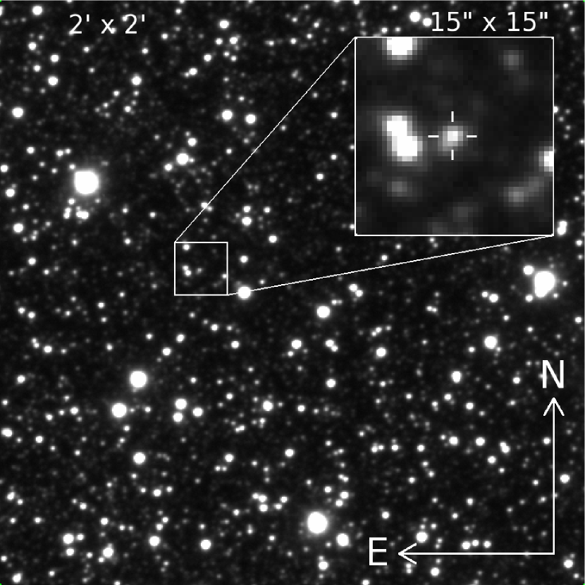
The microlensed source star of the event is located at $(\alpha,\delta)_{\rm J2000}=(17^{\rm h}57^{\rm m}47.72^{\rm s},-27^{\circ}23^{\prime}40^{\prime\prime}\hskip-2.0pt.3)$ in equatorial coordinates and $(l,b)=(2.70^{\circ},-1.52^{\circ})$ in Galactic coordinates (with the accuracy of the absolute position of the order of 0.1 arcsec). This region of the sky corresponds to the densest stellar region in the Galactic bulge toward which vast majority of microlensing events are being detected. Figure 1 shows the finding chart of the event taken in 2010 when the source had not yet been magnified. The brightness and color of the event at the baseline, calibrated to the standard $VI$ system, are $I=17.51$ and $V-I=3.03$, respectively.

Figure 1.— Finding chart for the microlensing event OGLE-2011-BLG-0265 as seen at the baseline level in 2010. The position of the source star (and the lens) is marked with the white cross, $(\alpha,\delta)_{\rm J2000}$ = $(17^{\rm h}57^{\rm m}47.72^{\rm s}$, $-27^{\circ}23^{\prime}40^{\prime\prime}\hskip-2.0pt.3)$ $\pm 0.1^{\prime\prime}$. The field of view is 2’ x 2’, while the inset covers 15” x 15”. Pixel scale is 0.26”/px. North is up and east is to the left. The brightest stars in the inset are $I\sim 16.2-16.4$, while the faintest visible at this scale are $I\sim 20$. The brightest star in the whole chart is TYC 6849-852-1 ($I\approx 11$).

The OGLE-IV survey is conducted using the 1.3-m Warsaw telescope equipped with the 32-CCD mosaic camera located at the Las Campanas Observatory in Chile. A single image covers approximately 1.4 square degrees with a resolution of 0.26 arcsec/pixel. OGLE-2011-BLG-0265 is located in the “BLG504” OGLE-IV field which was observed with 18-minute cadence in the 2011 season. See the OGLE Web page for the map of the sky coverage. The exposure time was 100 seconds and the variability monitoring was performed in the $I$-band filter. Several $V$-band images were also taken during the event in order to determine the color of the source star. The analyzed OGLE-IV data set of the event contains 3749 epochs covering three observing seasons 2010 – 2012.

The MOA project is regularly surveying the Galactic bulge with the 1.8-m telescope at the Mt. John Observatory in New Zealand. Images are collected with a ten-CCD mosaic camera covering $\approx 2.2$ square degrees. OGLE-2011-BLG-0265 lies in the high-cadence MOA field “gb10” which is typically visited a few times per hour, enabling to take 4774 epochs in total during the 2006-2012 seasons. Observations were conducted using the wide non-standard $R$/$I$ filter with the exposure time of 60 seconds.

OGLE-2011-BLG-0265 is also located in the footprint of the survey conducted at the Wise Observatory in Israel with the 1.0-m telescope and four-CCD mosaic camera, LAIWO (Shvartzvald & Maoz, 2012). This site fills the longitudinal gap between the OGLE and MOA sites enabling round-the-clock coverage of the event. In total 710 epochs were obtained from this survey. Observations were carried out with the $I$-band filter and the exposure time was 180 seconds.

OGLE-2011-BLG-0265 event turned out to evolve relatively slowly. Data collected by survey observations have good enough coverage of the anomaly and overall light curve to identify the planetary nature of the event. Nevertheless, the phenomenon was also monitored by several follow-up groups based on the anomaly alert issued on July 2, 2011 by the MOA group. It should be noted that the OGLE group generally does not issue alerts of ongoing anomalies in the present phase.

The groups that participated in the follow-up observations include the Probing Lensing Anomalies NETwork (PLANET: Beaulieu et al. 2006), Microlensing Follow-Up Network ($\mu$FUN: Gould et al. 2006), RoboNet (Tsapras et al., 2009), and MiNDSTEp (Dominik et al., 2010). Telescopes used for these observations include PLANET 1.0-m of South African Astronomical Observatory (SAAO) in South Africa, PLANET 0.6-m of Perth Observatory in Australia, $\mu$FUN 1.3-m SMARTS telescope of Cerro Tololo Inter-American Observatory (CTIO) in Chile, $\mu$FUN 0.4-m of Auckland Observatory in New Zealand, $\mu$FUN 0.36-m of Farm Cove Observatory (FCO) in New Zealand, $\mu$FUN 0.8-m of Observatorio del Teide in Tenerife, Spain, $\mu$FUN 0.6-m of Observatorio do Pico dos Dias (OPD) in Brazil, $\mu$FUN 0.4-m of Marty S. Kraar Observatory of Weizmann Institute of Science (Weizmann) in Israel, MiNDSTEp Danish 1.54-m telescope at La Silla Observatory in Chile, 2.0-m Liverpool Telescope at La Palma, RoboNet FTN 2.0-m in Hawaii, and RoboNet FTS 2.0-m in Australia.

By the time the first anomaly had ended, a series of solutions of lensing parameters based on independent real-time modeling were released. A consistent interpretation of these analyses was that the anomaly was produced by a planetary companion to the lens star. The models also predicted that there would be another perturbation in about ten days after the first anomaly followed by the event peak just after the second anomaly. Based on this prediction, follow-up observations were continued beyond the main anomaly up to the peak and even beyond. This enabled dense coverage of the second anomaly which turned out to be important for the precise characterization of the lens system. See Section 4.1.

The event did not return to its baseline until the end of the 2011 season – ${\rm HJD}^{\prime}(={\rm HJD}-2450000)\sim 5870$. In order to obtain baseline data, observations were resumed in the 2012 season that started on ${\rm HJD}^{\prime}\sim 5960$. Combined survey and follow-up photometry constitute a very continuous and complete data set with the very dense coverage of the planetary anomaly.

Figure 2.— Light curve of the microlensing event OGLE-2011-BLG-0265. Only a subset of data taken during the event is presented – lower signal-to-noise observations, as well as, data providing little constraint on the final solution are omitted. Colors of data points are chosen to match those of the labels of observatories. The solid curve superposed on the data points represents the best-fit model curve ($u_{0}>0$). The model curve for the $u_{0}<0$ solution would be visually indistinguishable. The two upper panels show the enlarged view of the major (${\rm HJD}\sim 2455746.5$) and minor ($\sim 2455757.5$) planetary perturbation regions (marked with arrows).

Data acquired from different observatories were reduced using photometry codes that were developed by the individual groups. The photometry codes used by the OGLE and MOA groups, developed respectively by Udalski (2003) and Bond et al. (2001), are based on the Difference Image Analysis method (Alard & Lupton, 1998). The PySIS pipeline (Albrow et al., 2009) was used for the reduction of the PLANET data and the Wise data. The $\mu$FUN data were processed using the DoPHOT pipeline (Schechter et al., 1993). For the RoboNet and MiNDSTEp data, the DanDIA pipeline (Bramich, 2008) was used.

To analyze the data sets obtained from different observatories, we rescale the reported uncertainties for each data set (cf. Skowron et al., 2011). The microlensing magnification significantly changes the brightness of the measured object during the event and it is often the case that the reported uncertainties by the automatic pipelines are underestimated by different amounts. To account for this, we first adjust uncertainties by introducing a quadratic term so that the cumulative distribution function of $\chi^{2}$ as a function of magnification becomes linear. We then rescale error bars so that $\chi^{2}$ per degree of freedom (dof) becomes unity for each data set, where the value of $\chi^{2}$ is derived from the best-fit solution. This process greatly helps to estimate uncertainties of the lensing parameters. It is done in an iterative manner using the full model (i.e., with effects of parallax and orbital motion taken into account).

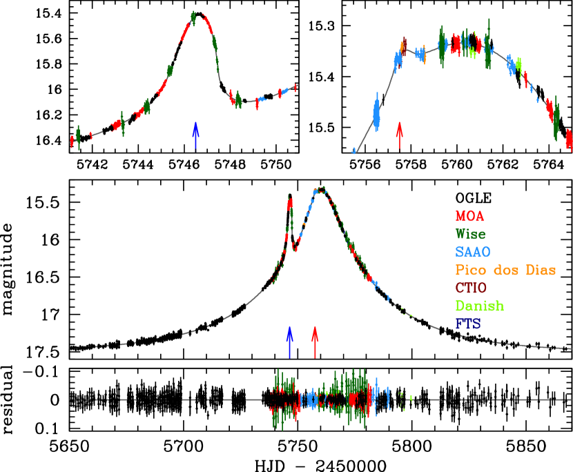
Figure 2 shows the light curve of OGLE-2011-BLG-0265. The subset of gathered data that were used in the final calculations is presented. For the most part, the light curve is well represented by a smooth and symmetric curve of a standard lensing event caused by a single-mass object (Paczyński, 1986) except for the short-term perturbations at ${\rm HJD}^{\prime}\sim 5746.5$ (major perturbation) and 5757.5 (minor perturbation), which lasted for $\sim 4$ days and $\sim 1$ day, respectively. These short-term perturbations are characteristic features of planetary microlensing (Mao & Paczyński, 1991; Gould & Loeb, 1992).

The dense temporal coverage from the multiple sites is useful in ensuring that there is no missing feature in the light curve. Also, overlapping observations allows to perform extensive self consistency checks among the data sets. After investigating residuals of all data sets used in the initial fits and correlating them with the observing conditions at the sites (seeing, sky background, and airmass), we carefully remove points for which we are less confident. Also, we do not use data sets that add no or little constrain to the light curve – such as data taken during only two or three nights of observations, or data taken during monotonic decline of the event after planetary anomalies. The procedure of keeping smaller number of confident data points allows us to limit influence of potential systematic errors and increase our confidence in the results, while, due to the redundancy of the gathered data, not harming the discriminatory power of the light curve.

3. Modeling The Light Curve

Planetary lensing is a special case of the binary lensing where the mass ratio between the lens components is very small. The description of a binary-lensing light curve requires seven basic parameters. The first three of these parameters characterize the geometry of the lens-source approach. These include the time scale for the source to cross the radius of the Einstein ring, $t_{\rm E}$ (Einstein time scale), the time of the closest source approach to a reference position of the lens system, $t_{0}$, and the lens-source separation at $t_{0}$, $u_{0}$ (impact parameter). For the reference position of the lens, we use the center of mass of the binary system. The Einstein ring denotes the image of a source for the case of the exact lens-source alignment. Its angular radius, $\theta_{\rm E}$ (Einstein radius), is commonly used as a length scale in describing the lensing phenomenon and the lens-source impact parameter $u_{0}$ is normalized to $\theta_{\rm E}$. Another three parameters needed to characterize the binary lens include: the mass ratio between the lens components, $q$, the projected binary separation in units of the Einstein radius, $s$, and the angle of the binary axis in respect to the lens-source relative motion, $\alpha$. The last parameter is the angular source radius $\theta_{*}$ normalized to $\theta_{\rm E}$, i.e., $\rho=\theta_{*}/\theta_{\rm E}$ (normalized source radius). This parameter is needed to describe the planet-induced perturbation during which the light curve is affected by the finite size of a source star (Bennett & Rhie, 1996).

In addition to the basic binary lensing parameters, several higher-order parameters are often needed to describe subtle light curve deviations. OGLE-2011-BLG-0265 lasted nearly throughout the whole Bulge season. For such a long time-scale event, the motion of the source with respect to the lens may deviate from a rectilinear motion due to the change of the observer’s position caused by the Earth’s orbital motion around the Sun and this can cause a long-term deviation in the light curve (Gould, 1992). Consideration of this, so called “parallax” effect, in modeling a microlensing light curve requires to include two additional parameters of $\pi_{{\rm E},N}$ and $\pi_{{\rm E},E}$, which represent the two components of the lens parallax vector $\mbox{\boldmath$\pi$}_{\rm E}$ projected on the sky in the north and east equatorial coordinates, respectively. The direction of the parallax vector corresponds to the relative lens-source motion in the frame of the Earth at a specific time ($t_{0,{\rm par}}$). We use $t_{0,{\rm par}}=2455760.1$. The size of the parallax vector is related to the Einstein radius $\theta_{\rm E}$ and the relative lens-source parallax $\pi_{\rm rel}={\rm AU}\,(D_{\rm L}^{-1}-D_{\rm S}^{-1})$ by

$$\pi_{\rm E}={\pi_{\rm rel}\over\theta_{\rm E}},$$ (1)

where $D_{\rm L}$ and $D_{\rm S}$ are the distances to the lens and source, respectively. Measurement of the lens parallax is important because it, along with the Einstein radius, allows one to determine the lens mass and distance to the lens as

$$M={\theta_{\rm E}\over\kappa\pi_{\rm E}}$$ (2)

and

$$D_{\rm L}={{\rm AU}\over\pi_{\rm E}\theta_{\rm E}+\pi_{\rm S}},$$ (3)

respectively (Gould, 1992). Here $\kappa=4G/(c^{2}{\rm AU})$ and $\pi_{\rm S}={\rm AU}/D_{\rm S}$ represents the parallax of the source star.

Table 1Lensing Parameters

parameter	u$\mathbf{{}_{0}>0}$ solution	$u_{0}<0$ solution
$\chi^{2}/{\rm dof}$	4381.0/4470	4386.7/4470
$t_{0}$ (${\rm HJD}^{\prime}$)	5760.0949 $\pm$ 0.0086	5760.0925 $\pm$ 0.0085
$t_{\rm eff}$ (days)	6.955 $\pm$ 0.017	-6.843 $\pm$ 0.031
$t_{\rm E}$ (days)	53.63 $\pm$ 0.19	53.33 $\pm$ 0.27
$t_{*}$ (days)	0.5248 $\pm$ 0.0055	0.5173 $\pm$ 0.0053
$q$ ($10^{-3}$)	3.954 $\pm$ 0.063	3.923 $\pm$ 0.059
$s_{0}$	1.03900 $\pm$ 0.00086	1.03790 $\pm$ 0.00085
$\alpha_{0}$ ($\deg$)	-27.15 $\pm$ 0.14	25.96 $\pm$ 0.23
$\pi_{{\rm E},N}$	0.238 $\pm$ 0.060	0.38 $\pm$ 0.11
$\pi_{{\rm E},E}$	0.042 $\pm$ 0.017	0.061 $\pm$ 0.016
$ds/dt$ (${\rm yr}^{-1}$)	0.354 $\pm$ 0.019	0.369 $\pm$ 0.019
$d\alpha/dt$ ($\deg\,{\rm yr}^{-1}$)	52.9 $\pm$ 6.3	-24.2 $\pm$ 7.7
$F_{\rm S,OGLE}$	1.860 $\pm$ 0.010	1.8380 $\pm$ 0.0096
$F_{\rm base,OGLE}$	1.92436 $\pm$ 0.00091	1.92519 $\pm$ 0.00087

Note. — ${\rm HJD}^{\prime}={\rm HJD}-2450000$. $\alpha_{0}$ and $s_{0}$ denote projected binary axis angle and separation for the epoch $t_{0,{\rm orb}}=2455748.0$, respectively. The reference position for the definition of $t_{0}$ and $u_{0}$ is set as the center of mass of the lens system. $t_{\rm eff}=u_{0}\cdot t_{\rm E}$. Geocentric reference frame is set in respect to the Earth velocity at $t_{0,{\rm par}}=2455760.1$. Flux unit for $F_{\rm S}$ and $F_{\rm base}$ is 18 mag – for the instrumental and $\sim 18.22$ for the calibrated OGLE I-band data. (See Fig. 3 for the lens geometry and Fig. 5 for the CMD).

Another effect that often needs to be considered in modeling long time-scale lensing events is the orbital motion of the lens (Albrow et al., 2000; Penny et al., 2011; Shin et al., 2011; Park et al., 2013). The lens orbital motion affects the light curve by causing both the projected binary separation $s$ and the binary axis angle $\alpha$ to change in time. It is especially important for the binary lensing systems whose separation on the sky is close to their Einstein ring radius (as we experience in this event). The shape of the emerging “resonant caustic” is very sensitive to the change of the binary separation. Also, such caustic is considerably larger than caustics produced by other lens configurations allowing larger part of the lens plane to be accurately probed during the event. We account for the orbital effect by assuming that the change rates of the projected binary separation, $ds/dt$, and the angular speed, $d\alpha/dt$, are constant. This is sufficient approximation as we expect the orbital periods to be significantly larger than the 11-day period between the perturbations seen in the light curve.

Since now the binary separation is a function of time, we quote at the tables and use as fit parameters the value of the binary separation ($s_{0}$) and the binary axis angle ($\alpha_{0}$) for a specific epoch: $t_{0,{\rm orb}}$. Here we choose $t_{0,{\rm orb}}$ to be 2455748.0. We closely follow conventions of the lensing parameters described in Skowron et al. (2011) with one difference; since we use $\alpha$ as an angle of the binary axis with respect to the lens-source trajectory, $d\alpha/dt$ describes the rotation of the binary axis in the plane of the sky.

The deviation in a lensing light curve caused by the orbital effect can be smooth and similar to the deviation induced by the parallax effect. Therefore, considering the orbital effect is important as it might affect the lens parallax measurement and thus the physical parameters of the lens (Batista et al., 2011; Skowron et al., 2011).

With the lensing parameters, we test different models of the light curve. In the first model (standard model), the light curve is fitted with use of the seven basic lensing parameters. In the second model (parallax model), we additionally consider the parallax effect by adding the two parallax parameters of $\pi_{{\rm E},N}$ and $\pi_{{\rm E},E}$. In the third model (orbit model), we consider only the orbital motion of the lens by including the orbital parameters $ds/dt$ and $d\alpha/dt$, but do not consider the parallax effect. In the last model (parallax+orbit model), we include both: the orbital motion of the lens and the orbital motion of the Earth (which give rise to the parallax effect).

For a basic binary model, every source trajectory has its exact mirror counterpart with respect to the star-planet axis – with $(u_{0},\alpha)\rightarrow-(u_{0},\alpha)$ being the only difference. However, when the additional effects are considered, each of the two trajectories with $u_{0}>0$ and $u_{0}<0$ deviate from a straight line and the pair of the trajectories are no longer symmetric. It is known that the models with $u_{0}>0$ and $u_{0}<0$ can be degenerate, especially for events associated with source stars located near the ecliptic plane – this is known as the “ecliptic degeneracy” (Skowron et al., 2011). For OGLE-2011-BLG-0265, the source star is located at $\beta\sim 2.7^{\circ}$ and thus we check both $u_{0}>0$ and $u_{0}<0$ solutions.

In modeling the OGLE-2011-BLG-0265 light curve, we search for the set of lensing parameters that best describes the observed light curve by minimizing $\chi^{2}$ in the parameter space. We conduct this search through three steps. In the first step, grid searches are conducted over the space of a set of parameters while the remaining parameters are searched by using a downhill approach (Dong et al., 2006). We then identify local minima in the grid-parameter space by inspecting the $\chi^{2}$ distribution. In the second step, we investigate the individual local minima found from the initial search and refine the individual local solutions. In the final step, we choose a global solution by comparing $\chi^{2}$ values of the individual local minima. This multi-step procedure is needed to probe the existence of any possible degenerate solutions. We choose $s$, $q$, and $\alpha$ as the grid parameters because they are related to the light curve features in a complex way such that a small change in their values can lead to dramatic changes in lensing light curves. On the other hand, the light curve shape depends smoothly on the remaining parameters and thus they are searched for by using a downhill approach. For the $\chi^{2}$ minimization for refinement and characterization of the solutions, we use the Markov Chain Monte Carlo (MCMC) method.

Figure 3.— Geometry of the lensing system and the source star trajectory projected onto the plane of the sky. The upper panel is for the best-fit solution with $u_{0}>0$ and the lower panel is for the $u_{0}<0$ solution. The $u_{0}>0$ solution provides a slightly better fit than the $u_{0}<0$ solution – by $\Delta\chi^{2}=5.7$. The closed figures with cusps represent the caustics at two different epochs: ${\rm HJD}^{\prime}=5746.5$ and 5757.5, which correspond to the moments of the major and minor perturbation in the light curve. The line with an arrow represents the source trajectory as seen from the Earth – the curvature of the line is due to the parallax effect. The small empty circles represent the size and positions of the source star at both epochs. Also marked are the positions of the planet (small dots on the right) and its host star (big dots on the left) – the displacement of the planet due to its orbital motion over 11 days between the perturbations is clearly visible. Origin is at the Center of Mass of the planetary system. The horizontal axis is parallel with the star-planet axis at the time $t_{0}$.

Figure 4.— Cumulative $\chi^{2}$ distributions as a function of a data point number for three microlensing models. The vertical bands mark the time of the major and minor planetary anomaly. We see, that the minor anomaly cannot be a well fitted without the inclusion of the lens orbital motion. Two anomalies appeared in the light curve closer in time than could be fitted with a static binary model. Since the first anomaly is extremely well covered with observations, it is the second anomaly that does not fit the best possible static model.

A planetary perturbation is mostly produced by the approach of the source star close to caustics that represent the positions on the source plane at which the lensing magnification of a point source becomes infinite. During the approach, lensing magnifications are affected by finite-source effects due to the differential magnification caused by the steep gradient of magnification pattern around the caustic. For the computation of finite-source magnifications, we use the ray-shooting method (Schneider & Weiss, 1986; Kayser et al., 1986; Wambsganss, 1997). In this method, a large number of rays are uniformly shot from the image plane, bent according to the lens equation, and land on the source plane. The lens equation for image mapping from the image plane to the source plane is expressed as

$$\zeta=z-{1\over 1+q}\left({1\over\bar{z}-\bar{z}_{{\rm L},1}}+{q\over\bar{z}-\bar{z}_{{\rm L},2}}\right),$$ (4)

where $\zeta$, $z_{\rm L}$, and $z$ are the complex notations of the source, lens and image positions, respectively, and the overbar denotes complex conjugate. Here all lengths are expressed in units of the Einstein radius. The finite magnification is computed as the ratio of the number density of rays on the source surface to the density on the image plane. This numerical technique requires heavy computation and thus we limit finite-magnification computation based on the ray-shooting method to the region very close to caustics. In the adjacent region, we use a hexadecapole approximation, with which finite magnification computation can be faster by several orders of magnitude (Pejcha & Heyrovský, 2009; Gould, 2008). We solve lens equation by using the complex polynomial method described in Skowron & Gould (2012).

In computing finite-source magnifications, we incorporate the limb-darkening variation of the stellar surface brightness. The surface brightness profile is modeled as $S_{\lambda}\propto 1-c_{\lambda}\cdot(1-\cos\phi)-d_{\lambda}\cdot(1-\sqrt{\cos\phi})$, where $c_{\lambda}$ and $d_{\lambda}$ are the limb-darkening coefficients of the wavelength band $\lambda$ and $\phi$ is the angle between the normal to the stellar surface and the line of sight toward the center of the star. Based on the stellar type (see Section 5), we adopt the coefficients using Table 32 (square-root law) of Claret (2000) for $v_{\rm t}=2$, solar metallicity, $T_{\rm eff}=5000\,{\rm K}$ and $\log g=3.5$:

$$c_{I-band},\,d_{I-band} =0.2288,\,0.4769,$$ (5)

$$c_{MOA-R},\,d_{MOA-R} =0.2706,\,0.4578,$$ (6)

$$c_{V-band},\,d_{V-band} =0.5337,\,0.2993.$$ (7)

Here the values for the non-standard MOA-R filter are taken as linear combination of R-band and I-band coefficients with 30% and 70% weights.

4. Results

4.1. Best-fit Solution

In Table 1, we present the best-fit solutions along with their $\chi^{2}$ values. In order to provide information about the blended light (i.e., the light that was not magnified during the event), we also present the source, $F_{\rm S}$, and baseline, $F_{\rm base}$, fluxes estimated from the OGLE photometry. We note that the uncertainty of each parameter is estimated based on the distribution in the MCMC chain obtained from modeling.

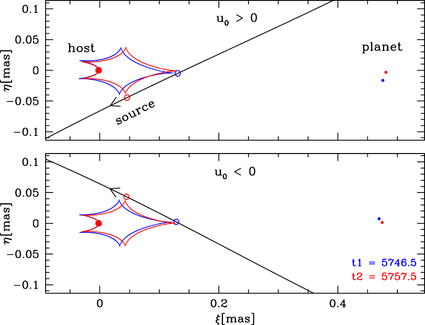
It is found that the perturbation was produced by a planetary companion with a planet/star mass ratio $q\sim 3.9\times 10^{-3}$ located close to the Einstein ring of its host star, i.e, $s\sim 1.0$. In the upper panel of Figure 3, we present the locations of the lens components, the caustic, and the source trajectory for the best-fit solution. Since the planet is close to the Einstein ring, the resulting caustic forms a single closed curve with six cusps. It is found that the major (at ${\rm HJD}^{\prime}=5746.5$) and minor (at ${\rm HJD}^{\prime}=5757.5$) perturbations in the lensing light curve were produced by the approach of the source star close to the strong and weak cusps of the caustic, respectively.

We find that the event suffers from the ecliptic degeneracy. In Figure 3, we compare the lens-system geometry of the two degenerate solutions with $u_{0}<0$ and $u_{0}>0$. We note that the source trajectories of the two degenerate solutions are almost symmetric with respect to the star-planet axis. The $\chi^{2}$ difference between the two degenerate models is merely 5.7 – with $u_{0}>0$ solution slightly preferred over the $u_{0}<0$ solution. We further discuss this degeneracy in Section 5.2.

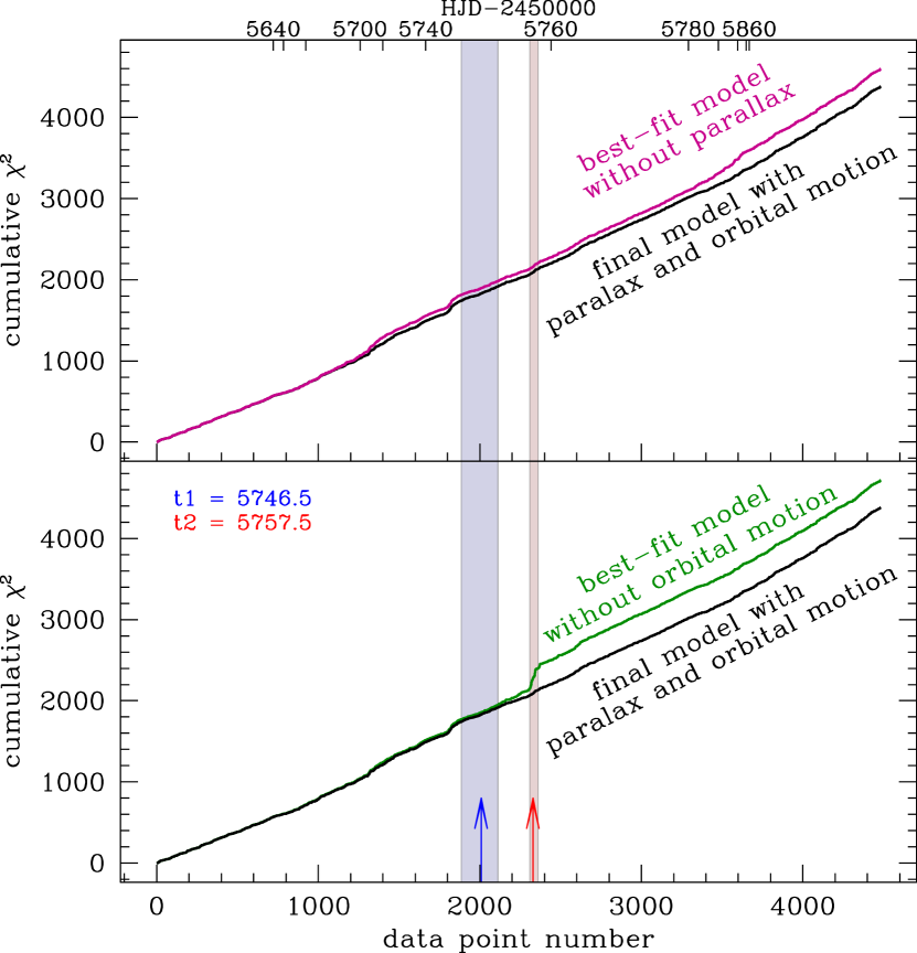
Higher-order effects are important for the event. We find that the model considering the parallax effect improves the fit with $\Delta\chi^{2}=230.9$ for $u_{0}>0$ and 127.8 for $u_{0}<0$ compared to the standard model. The model considering the lens orbital motion (but without parallax) improves the fit even more with $\Delta\chi^{2}=349.1$ compared to the standard model. Considering both the parallax and orbital effects yields a light curve model that fits the data significantly better with $\Delta\chi^{2}=559.4$ for $u_{0}>0$ and 565.1 for $u_{0}<0$ relative to the standard model.

The importance of the lens orbital motion can be seen in Figure 4. It shows cumulative $\chi^{2}$ distribution for the full (final) model and compares it to the models without the parallax effect (upper panel) and without the lens orbital motion (lower panel) taken into account. It is found that the signal of the orbital effect is mainly seen from the part of the light curve at around ${\rm HJD}^{\prime}\sim 5757.5$, which corresponds to the time of the minor anomaly. The second anomaly happened sooner than predicted by the static binary model. Without the observations at this time, we would have lacked the information on the evolution of the the caustic shape during the time between the anomalies. The minor anomaly was densely covered by follow-up data, especially the SAAO data, but the coverage by the survey data is sparse. As a result, the orbital parameters could not be well constrained by the survey data alone.

Figure 5.— Location of the source star in the OGLE color-magnitude diagram for stars in the $1.5^{\prime}\times 1.5^{\prime}$ field centered on the lensing event. Also shown is the centroid of the red clump giant stars that is used to calibrate the brightness and color of the source star. Light seen before and after the event (baseline level) was separated into the “source” and the “blend” light (or the portion of light that was magnified and the portion that was not magnified during the course of the event, respectively)

.

4.2. Angular Einstein radius

Detection of the microlens parallax enables the measurement of the mass and distance to the planetary system. The Einstein radius, the second component required by Equations (2) and (3), is estimated by $\theta_{\rm E}=\theta_{*}/\rho$, where the angular source radius $\theta_{*}$ is obtained from the color and brightness information and the normalized source radius $\rho$ is measured from the microlensing light curve fitting to the planetary perturbation.

4.2.1 Intrinsic color and extinction-corrected brightness of the source star

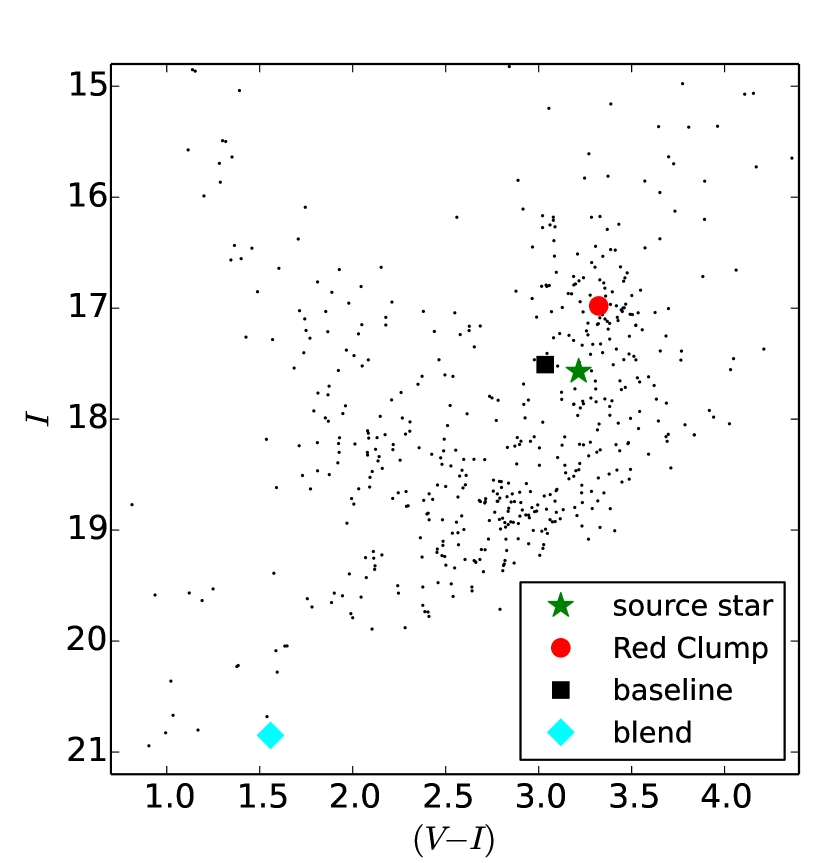
To determine the angular source radius, we first locate the source star on the color-magnitude diagram for stars in the field and then calibrate its de-reddened color and brightness by using the centroid of the red clump giants as a reference under the assumption that the source and red clump giants experience the same amount of extinction and reddening (Yoo et al., 2004).

In Figure 5, we present the location of the source star in the color-magnitude diagram. Using the method of Nataf et al. (2010) finding the centroid of the red clump in the 1.5’ x 1.5’ region of the sky around the source star, we estimate that the source star (with $V=20.77$ and $I=17.57$) is $0.12$ mag bluer and $0.59$ mag fainter than the typical red clump giant, and hence, is most likely also a K-type giant star located in the Galactic bulge. Based on the intrinsic color of the red clump giant stars $(V-I)_{{\rm RC},0}=1.06$ (Bensby et al., 2011), we estimate the de-reddened color of the source star to be $(V-I)_{{\rm S},0}=0.94$.

With the observed ($(V-I)_{\rm RC}=3.32$) and intrinsic colors of the red clump stars, we estimate the total reddening toward the Galactic Bulge:

$$E(V-I)=(V-I)_{\rm RC}-(V-I)_{{\rm RC},0}=3.32-1.06=2.26.$$ (8)

From Nataf et al. (2013) the mean distance to the Galactic bulge stars in the direction of the event is 7.8 kpc and the intrinsic brightness of the red clump stars is $M_{I,{\rm RC},0}=-0.11$. With the measured observed brightness $I_{\rm RC}=16.98$, we estimate the extinction to the bulge to be $A_{I}=2.63$. This is consistent with the estimated reddening of 2.26 as the slope of the reddening vector ($\partial A_{I}/\partial E(V-I)$) is typically $\sim 1.2$, and in most cases is between 1.0 and 1.4 for the Galactic bulge sight lines (Nataf et al., 2013, Figure 7). The extinction in the $V$ band is calculated as $A_{V}=A_{I}+E(V-I)=4.89$. Then, the extinction-corrected magnitudes of the source star are computed as

$$V_{{\rm S},0} =V_{\rm S}-A_{V}=20.77-4.89=15.88,$$ (9)

$$I_{{\rm S},0} =I_{\rm S}-A_{I}=17.57-2.63=14.94.$$ (10)

4.2.2 Uncertainties of the source color estimation

Although uncertainties of the observed color and brightness of the source stars are typically low (in this case 0.01 mag), the uncertainty in the centroiding of the red clump and the differential reddening in the field causes that the true intrinsic colors of the microlensing sources are typically known with lower accuracy. Bensby et al. (2013, Section 3.2) compare the colors of source stars of the 55 microlensing events determined with both spectroscopic and microlensing techniques. Their Figure 5 shows that the disagreement between the two estimations is typically 0.07 mag for the blue star sample and 0.08 mag for all stars. There is no physical reason for the measurement of the color offset from the red clump stars to be less accurate for red stars than for blue stars. Hence, the authors point to, clearly but not perfectly, the color-$T_{\rm eff}$ relations as the source of the increased scatter for red stars (with $T_{\rm eff}<5500$ K, cf. Bensby et al. 2013, Figure 7). The observed 0.07 mag scatter between the spectroscopic and microlensing color estimates also includes the uncertainties in $T_{\rm eff}$, which are of the order of $100$ K and would generate $\sim 0.034$ mag uncertainty in color (compare with Table 5 and Figure 7 of Bensby et al. 2013). By subtracting this source of scatter in quadrature from the observed scatter, we obtain 0.061 mag, which still contains some unknown uncertainty of the stellar models themselves.

The sample of events analyzed by Bensby et al. (2013) also contains some problematic events of two types. One type are the events where the coverage of the light curve in the multiple photometric bands was not sufficient to accurately determine observed color, while the other type are the events in the fields with poorly defined red clumps. This allows us to argue that for well observed microlensing events in the fields with well defined red clump, the typical error in the microlensing color estimation is on the order of $0.05$ mag.

One could worry that the assumption of a typical error of the intrinsic color estimation does not take into account the influence of the differential reddening, which in fact, varies from field to field. Figure 6 of Bensby et al. (2013) addresses this issue, showing that there is no evidence of strong correlation between the differential reddening in the fields of 55 events (as measured by Nataf et al. (2013)) and errors in their color estimations. This actually could be understood by realizing that the dominating source of scatter in the observed colors of red clump stars comes from the gradient of the reddening across the field. This gradient, however, has no effect on the position of the red clump stars centroid.

As an example, we took samples of stars from four circles centered on our event with the diameters of 1.5’, 2’, 3’, and 4’, respectively, and used them to measure the centroid of the red clump. All four measurements are within 0.02 mag of each other, even though the measure of the differential reddening (as defined by Nataf et al. 2013) is between 0.16 and 0.24 in these circles.

It is also worth noting that any error in the relative position of the source star from the centroid of the red clump that could come from the differential reddening would only partially contribute to the final estimation of the angular size of the star. As we will see in the following section, the calibration of the angular radius of the star contains two terms with opposite signs: $\sim 0.5(V-I)_{0}-0.2I_{0}$ (Eq. (11)). More dust in front of the star influences both estimations of $(V-I)_{0}$ and $I_{0}$ in the same direction, and since $A_{I}\approx 1.2\,E(V-I)$, the overall error that comes from the wrong estimation of the reddening is reduced by 50% ($1.2\times 0.2/0.5=0.5$).

The OGLE-2011-BLG-0265 event is located $1.5\deg$ from the Galactic plane in the region strongly obscured by the interstellar dust ($E(V-I)=2.26$) and affected by the differential reddening. Following Nataf et al. (2013), we calculate the measure of the differential reddening ($\sigma_{E(V-I)}$) in the $1.5^{\prime}\times 1.5^{\prime}$ patch of the sky around the event. The observed $V-I$ colors of the red clump stars show $0.20$ mag dispersion, which leads to the estimation of $\sigma_{E(V-I)}=0.16$ mag. However, having the evidence for at most minor influence of the differential reddening on the final estimation of the color, and knowing that only half of the error (due to reddening) enters the final result, we only slightly increase our uncertainty of the color from 0.05 to 0.06 mag due to the heavily reddened field.

We expect the error in the estimation of $I_{0}$ to be slightly higher than the assumed error for $(V-I)_{0}$. In order to measure the observed brightness of the red clump, the luminosity function of the red giant branch has to be fitted simultaneously with the luminosity function of the red clump giants. Based on the reproducibility of the red clump centroiding under various assumptions regarding the red giant branch luminosity function, we conservatively assume 0.1 magnitude error in the estimation of $I_{0}$ of the source star.

4.2.3 Angular size from the surface brightness relations

Knowing the dereddened color of the star and the extinction-corrected brightness enables the use of the surface brightness relation to find the angular radius ($\theta_{*}$). We note that in microlensing we typically measure $(V-I)_{0}$ color, hence, ideally we would like to use a calibration based on this quantity. By including the additional transformation process from $(V-I)_{0}$ to $(V-K)_{0}$, the uncertainty of the estimated color increases by a factor 1.5 – 2.5 (for example $\partial(V-K)/\partial(V-I)\approx 2.5$ for stars with $(V-I)<1.3$ (Bessell & Brett, 1988)). Kervella & Fouqué (2008) provide such a relation calibrated with dwarfs and subgiant stars; we write:

$$\log\theta_{*}=3.1982-0.2I_{0}+0.4895(V-I)_{0}-0.0657(V-I)_{0}^{2},$$ (11)

where the angular radius is given in $\mu$as and the scatter of the relation is 0.0238. The relation in $(V-K)$ for the same types of stars based on Kervella et al. (2004) is

$$\log\theta_{*}=3.2165-0.2V_{0}+0.2753(V-K)_{0}$$ (12)

and the quadratic relation for the wider range of stars was given by Di Benedetto (2005):

$$\log\theta_{*}=3.2120-0.2V_{0}+0.2968(V-K)_{0}-0.0088(V-K)_{0}^{2}.$$ (13)

Kervella & Fouqué (2008) believe that the scatter around the provided relation is dominated by the intrinsic scatter rather than measurement errors. This yields the relative uncertainty of the angular radius at 5.5%. Calibrations based on an infrared color have much smaller intrinsic scatter, so careful removal of scatter due to measurement error is required. Kervella et al. (2004) estimate the intrisic scatter around the provided relation is 1%, whereas Di Benedetto (2005) estimates 1.8% and argues that the accuracy of the star sizes obtained from the infrared-based surface brightness relations is $<2\%$, but higher than the 1% estimated by Kervella et al. (2004).

We note that despite having much smaller scatter, the relations with $(V-K)_{0}$ (transformed from $(V-I)_{0}$) yield higher uncertainty of the angular radius than the relation originally calibrated in $(V-I)_{0}$, unless the accuracy of $(V-I)_{0}$ estimation is $\lesssim 0.05$ or $(V-I)_{0}>1.3$, where the slope of $(V-K)$ vs $(V-I)$ is more shallow. Hence, we use Kervella & Fouqué (2008) relation in the OGLE-2011-BLG-0265 case, which leads to the final estimation of the angular source radius

$$\theta_{*}=4.09\pm 0.41\ \mu{\rm as}.$$ (14)

Combining the physical and the normalized source radius yields the Einstein radius of $\theta_{\rm E}=\theta_{*}/\rho=0.42\pm 0.04$ mas (for both $u_{0}>0$ and $u_{0}<0$ solutions of the parallax+orbit model).

4.3. Physical Parameters

With the measured Einstein radius and the lens parallax, we are able to estimate the physical quantities of the lens system (Table 2). For the best-fit solution ($u_{0}>0$, parallax+orbit model), the lens mass and distance to the lens are $M=0.22\pm 0.06\ M_{\odot}$ and $D_{\rm L}=4.4\pm 0.5$ kpc, respectively. The mass of the planet is $M_{\rm p}=0.9\pm 0.3\ M_{\rm J}$. The projected separation between the host star and the planet is $a_{\perp}=1.9\pm 0.2$ AU and thus the planet is located well beyond the snow line of the host star.

For the marginally disfavored $u_{0}<0$ solution, the resulting physical parameters of the lens system are somewhat different – as expected, mainly caused by the difference in the north component of the parallax vector, i.e., $\pi_{{\rm E},N}$. See Table 1. In this case, the lens mass and distance are $M=0.14\pm 0.06\ M_{\odot}$ and $D_{\rm L}=3.5\pm 0.7$ kpc, respectively, and the mass of the planet is $M_{\rm p}=0.6\pm 0.3\ M_{\rm J}$.

Hence, the system belongs to a little-known population of planetary systems where a Jupiter mass planet orbits an M dwarf beyond its snow line.

Table 2Physical Lens Parameters

quantity	u$\mathbf{{}_{0}>0}$ solution	$u_{0}<0$ solution
$\theta_{\rm E}$ (mas)	$0.419\pm 0.040$	$0.423\pm 0.040$
$\mu_{\rm geo}$ (mas/yr)	$2.85\pm 0.29$	$2.89\pm 0.29$
$\mu_{{\rm hel},N}$ (mas/yr)	$2.72\pm 0.30$	$2.73\pm 0.32$
$\mu_{{\rm hel},E}$ (mas/yr)	$1.06_{-0.18}^{+0.29}$	$1.39_{-0.16}^{+0.19}$
$M_{\rm p}$ ($M_{\rm J}$)	$0.88_{-0.18}^{+0.27}$	$0.56_{-0.13}^{+0.25}$
$M_{\rm h}$ ($M_{\odot}$)	$0.211_{-0.045}^{+0.068}$	$0.136_{-0.031}^{+0.061}$
$D_{\rm L}$ (kpc)	$4.38_{-0.45}^{+0.51}$	$3.49_{-0.49}^{+0.71}$
$a_{\perp}$ (AU)	$1.89_{-0.20}^{+0.25}$	$1.51_{-0.20}^{+0.31}$
${\rm(KE/PE)}_{\perp}$	$0.387\pm 0.075$	$0.112\pm 0.060$

Note. — Parameters calculated for parallax+orbital model; $\theta_{\rm E}$: angular Einstein radius, $\mu_{\rm geo}$ and $\mu_{\rm hel}$: relative lens-source proper motion in the geocentric and heliocentric reference frames, respectively, $M_{\rm p}$: mass of the planet, $M_{\rm h}$: mass of the host star, $D_{\rm L}$: distance to the lens, $a_{\perp}$: projected star-planet, ${\rm(KE/PE)}_{\perp}$: the ratio of the transverse kinetic to potential energy.

5. Discussion

5.1. Degeneracy of the Microlensing Models

While the planetary nature of the perturbation in the OGLE-2011-BLG-0265 light curve is obvious, the event suffers from the orbiting binary ecliptic degeneracy (Skowron et al., 2011, see Appendix 3). The two solutions, $u_{0}<0$ and $u_{0}>0$, have nearly identical mass ratio $q=3.9\times 10^{-3}$, normalized separation $s=1.04$, Einstein radius $\theta_{\rm E}=0.42\,$ mas, and hence planet-host angular separation $\theta_{\perp}=0.44\,$ mas. They differ in the microlens parallax, especially in the north component $\pi_{{\rm E},N}=0.24$ ($u_{0}>0$) versus $\pi_{{\rm E},N}=0.38$ ($u_{0}<0$), and also in $d\alpha/dt$, which is often strongly correlated with $\pi_{{\rm E},N}$ (Batista et al., 2011; Skowron et al., 2011). This difference is important because it leads to a different mass and distance of the host $(M_{*}/M_{\odot},D_{\rm L}/{\rm kpc})=(0.22,\,4.4)$ versus (0.14, 3.5) for the $u_{0}>0$ and $u_{0}<0$ solutions, respectively.

The $u_{0}>0$ solution is favored by $\Delta\chi^{2}=5.7$ corresponding to a (frequentist) likelihood ratio of $\exp(5.7/2)=17$. This would be compelling evidence if treated at face value. However, it is known that the photometry of microlensing events occasionally suffers from low-level systematic trends at $\Delta\chi^{2}\sim$ few level.

As an additional way to resolve the degeneracy, we check the ratio of the projected kinetic to potential energy (Dong et al., 2009) estimated by

$$\beta=\biggl{(}{\rm KE\over PE}\biggr{)}_{\perp}={v_{\perp}^{2}r_{\perp}\over 2GM_{\rm tot}}={\kappa M_{\odot}{\rm yr}^{2}\over 8\pi^{2}}{\pi_{\rm E}s^{3}\gamma^{2}\over\theta_{\rm E}(\pi_{\rm E}+\pi_{S}/\theta_{\rm E})^{3}},$$ (15)

where $\gamma^{2}=(ds/dt/s)^{2}+(d\alpha/dt)^{2}$. For typical viewing angles, one expects $\beta\sim{\cal O}(0.4)$, as is the case for the $u_{0}>0$ solution. On the other hand, the lower value $\beta\sim 0.11$ (as in the $u_{0}<0$ solution) implies either that the planet is seen projected along the line of sight at the viewing angle $\psi\sim 2\beta\sim 0.22$ (corresponding to semi-major axis $a\sim a_{\perp}/(2\beta)\sim 4.5a_{\perp}$), or that we have just seen the planet when majority of its motion is directly toward (or away from) us. Of course, the prior probability of the first configuration for a point randomly distributed on a sphere is just $2\beta^{2}\sim 0.025$ and the probability for the second is similar.

However, while it is certainly true that the prior probability for any given planet’s position is uniform over a sphere, this is not the case for planets found by microlensing, which are preferentially detected within a factor $\sim 1.5$ of the Einstein radius (Gould & Loeb, 1992; Gould et al., 2010). First, since the planet actually lies very near the Einstein radius, it would have been detected in almost any angular orientation $\alpha$, so that the actual probability is more like $\beta$ than $\beta^{2}$, i.e., about 0.11. In addition, since giant planets around M dwarfs are a new class of planets, we do not know their distribution. It could be that the great majority of such planets lie at $a\sim 20\,$AU. Then, whenever these were found in planet-host microlensing events, they would have a very low value $\beta$. On the other hand, whenever we detect them at typical viewing angles, they will be considered as “free floating planets” (Sumi et al., 2011). Hence, the measurement of a low $\beta$ value is not a strong statistical argument against the $u_{0}<0$ solution which still remains as a viable option.

In summary, although both light curve and energy considerations point to the $u_{0}>0$ solution, it is difficult to confidently resolve the degeneracy between the two possible models based on the currently available data. Fortunately, the difference in the physical parameters estimated from the two degenerate solutions are not big enough to affect the conclusion that the lens belongs to a new class of giant planets around low-mass stars.

5.2. Prospects for Follow-up Observations

It will eventually be possible to confidently resolve the current degeneracy issue on the models of OGLE-2011-BLG-0265 when the Giant Magellan Telescope (GMT) comes on line in about 10 years. At that time, the source and lens will be separated by about 40 mas, or roughly 3 FWHM in the $J$-band. There are three observables that can then be used to distinguish the two solutions. First, the $u_{0}<0$ solution predicts a fainter lens because it has a lower mass. Second, it predicts slightly higher heliocentric proper motion (mainly in the East sky direction). Third, it predicts a different angle of the proper motion.

Each of these measurements has some potential problems. The prediction of the lens flux is influenced not only by the mass and the distance but also by the extinction to the lens. There is a substantial error in $\theta_{\rm E}$ that impacts the brightness in the same direction as the mass and distance. That is, if $\theta_{\rm E}$ is higher than we have estimated, then the distance is closer (so the lens is brighter) and the mass is greater (so the lens is brighter again). Fortunately, the detection of the lens will itself enable to measure the proper motion $\mu_{\rm hel}$ and therefore also the Einstein radius (see below). Also, with a bigger telescope, it will be possible to better estimate $\theta_{\rm E}$ by detailed characterization of the source star, thus, more accurate estimation of the $\theta_{*}$ then in Eq (14).

As can be seen from Table 2, the predictions for heliocentric proper motion differ by only $1\sigma$. This is the same problem as just mentioned: the proper motion prediction contains the significant error of $\theta_{\rm E}$.

By contrast, the angle of heliocentric proper motion, $\phi_{\mu}$, does not depend on $\theta_{\rm E}$. In terms of observables,

$$\mbox{\boldmath$\mu$}_{\rm hel}={\theta_{\rm E}\over t_{\rm E}}\,{\mbox{\boldmath$\pi$}_{\rm E}\over\pi_{\rm E}}+{{\bf v}_{\oplus,\perp}\over{\rm AU}}\pi_{\rm rel}=\theta_{\rm E}\biggl{(}{1\over t_{\rm E}}{\mbox{\boldmath$\pi$}_{\rm E}\over\pi_{\rm E}}+{{\bf v}_{\oplus,\perp}\over{\rm AU}}\pi_{\rm E}\biggr{)},$$ (16)

where ${\bf v}_{\oplus,\perp}$ is the motion of Earth projected on the sky at the fiducial time of the event $(v_{\oplus,N},v_{\oplus,E})=(-0.42,5.45)\,$AU/yr. This means that the position angle (North through East) is

$$\phi_{\mu}={\rm atan}{\pi_{{\rm E},E}+\pi_{\rm E}^{2}v_{\oplus,E}t_{\rm E}/{\rm AU}\over\pi_{{\rm E},N}+\pi_{\rm E}^{2}v_{\oplus,N}t_{\rm E}/{\rm AU}},$$ (17)

which is indeed independent of $\theta_{\rm E}$. We find $\phi_{\mu}=20.8_{-2.7}^{+5.3}\deg$ for $u_{0}>0$ and $\phi_{\mu}=26.4_{-1.2}^{+2.0}\deg$ for $u_{0}<0$. Thus if the actual measurement is $\phi_{\mu}=21^{\circ}$, it will strongly exclude $(4\,\sigma)$ the $u_{0}<0$ solution, but if it is $\phi_{\mu}=26^{\circ}$ then it will only marginally favor $(1\,\sigma)$ the $u_{0}<0$ solution.

Nevertheless, with three pieces of information, there is a good chance that the ensemble of measurements will favor one solution or the other.

6. Conclusions

We reported the discovery of a planet detected by analyzing the light curve of the microlensing event OGLE-2011-BLG-0265. It is found that the lens is composed of a giant planet orbiting a M-type dwarf host. Unfortunately, the microlensing modeling yields two degenerate solutions, which increase our uncertainties in mass of and distance to this planetary system and cannot be distinguished with currently available data. Planet-host mass ratio is, however, very well measured at $0.0039$.

The slightly preferred solution yields a Jupiter-mass planet orbiting a $0.22M_{\odot}$ dwarf. The second solution yields a 0.6 Jupiter-mass planet orbiting a $0.14M_{\odot}$ dwarf. There are good prospects for lifting the degeneracy of the solutions with future additional follow-up observations. In either case, OGLE-2011-BLG-0265 event demonstrates the uniqueness of the microlensing method in detecting planets around low-mass stars.

References

- Alard & Lupton (1998) Alard, C., & Lupton, R. H. 1998, ApJ, 503, 325
- Albrow et al. (2000) Albrow, M. D., Beaulieu, J.-P., Caldwell, J. A. R., et al. 2000, ApJ, 534, 894
- Albrow et al. (2009) Albrow, M. D., Horne, K., Bramich, D. M., et al. 2009, MNRAS, 397, 2099
- Batista et al. (2011) Batista, V., Gould, A., Dieters, S., et al. 2011, A&A, 529, A102
- Beaulieu et al. (2006) Beaulieu, J.-P., Bennett, D. P., Fouqué, P., et al. 2006, Nature, 439, 437
- Bennett & Rhie (1996) Bennett, D. P., & Rhie, S. H. 1996, ApJ, 472, 660
- Bennett et al. (2008) Bennett, D. P., Bond, I. A., Udalski, A., et al. 2008, ApJ, 684, 663
- Bennett et al. (2010) Bennett, D. P., Rhie, S. H., Nikolaev, S., et al. 2010, ApJ, 713, 837
- Bensby et al. (2011) Bensby, T., Adén, D., Meléndez, J., et al. 2011, A&A, 533, AA134
- Bensby et al. (2013) Bensby, T. Yee, J.C., Feltzing, S. et al. 2013, A&A, 549A, 147
- Bessell & Brett (1988) Bessell, M. S., & Brett, J. M. 1988, PASP, 100, 1134
- Bond et al. (2001) Bond, I. A., Abe, F., Dodd, R. J., et al. 2001, MNRAS, 327, 868
- Bonfils et al. (2011) Bonfils, X., Gillon, M., Forveille, T., et al. 2011, A&A, 528, 111
- Borucki et al. (2011) Borucki, W. J., Koch, D. G., Basri, G., et al. 2011, ApJ, 736, 19
- Boss (2006) Boss, A. P. 2006, ApJ, 643, 501
- Bramich (2008) Bramich, D. M. 2008, MNRAS, 386, L77
- Cassan et al. (2012) Cassan, A., Kubas, D., Beaulieu, J.-P., et al. 2012, Nature, 481, 167
- Charbonneau et al. (2009) Charbonneau, D., Berta, Z. K., & Irwin, J. 2009, Nature, 462, 891
- Claret (2000) Claret, A. 2000, A&A, 363, 1081
- Delfosse et al. (1998) Delfosse, X., Forveille, T., Mayor, M., Perrier, C., Naef, D., & Queloz, D. 1998, A&A, 338, L67
- Di Benedetto (2005) Di Benedetto, G. P. 2005, MNRAS, 357, 174
- Dominik et al. (2010) Dominik, M., Jørgensen, U. G., Rattenbury, N. J., et al. 2010, Astronomische Nachrichten, 331, 671
- Dong et al. (2006) Dong, S., DePoy, D. L., Gaudi, B. S., et al. 2006, ApJ, 642, 842
- Dong et al. (2009) Dong, S., Gould, A., Udalski, A., et al. 2009, ApJ, 695, 970
- Gaudi et al. (2008) Gaudi, B. S., Bennett, D. P., Udalski, A., et al. 2008, Science, 319, 927
- Gillon et al. (2007) Gillon, M., Pont, F., Demory, B.-O., et al. 2007, A&A, 472, L13
- Gould (1992) Gould, A. 1992, ApJ, 392, 442
- Gould & Loeb (1992) Gould, A., & Loeb, A. 1992, ApJ, 396, 104
- Gould (2008) Gould, A. 2008, ApJ, 681, 1593
- Gould et al. (2006) Gould, A., Udalski, A., An, D., et al. 2006, ApJ, 644, L37
- Gould et al. (2010) Gould, A., Dong, Subo, Gaudi, B. S, et al. 2010, ApJ, 720, 1073
- Ida & Lin (2005) Ida, S., & Lin, D. N. C. 2005, ApJ, 626, 1045
- Kains et al. (2013) Kains, N., Street, R. A., Choi, J.-Y., et al. 2013, A&A, 552, A70
- Kayser et al. (1986) Kayser, R., Refsdal, S., & Stabell, R. 1986, A&A, 166, 36
- Kervella et al. (2004) Kervella, P., Thévenin, F., Di Folco, E., & Ségransan, D. 2004, A&A, 426, 297
- Kervella & Fouqué (2008) Kervella, P., & Fouqué, P. 2008, A&A, 491, 855
- Kubas et al. (2012) Kubas, D., Beaulieu, J.-P., Bennett, D. P., et al. 2012, A&A, 540, 78
- Laughlin et al. (2004) Laughlin, G., Bodenheimer, P., & Adams, F. C. 2004, ApJ, 612, L73
- Mao & Paczyński (1991) Mao, S., & Paczyński, B. 1991, ApJ, 374, L37
- Marcy et al. (1998) Marcy, G. W., Butler, R. P., Vogt, S. S., Fischer, D., & Lissauer, J. J. 1998, ApJ, 505, L147
- Montet et al. (2014) Montet, B. T., Crepp, J. R., Johnson, J. A., Howard, A. W., & Marcy, G. W. 2014, ApJ, 781, 28
- Nataf et al. (2010) Nataf, D. M., Udalski, A., Gould, A., Fouqué, P., & Stanek, K. Z. 2010, ApJ, 721, L28
- Nataf et al. (2013) Nataf, D. M., Gould, A., Fouqué, P., et al. 2013, ApJ, 769, 88
- Paczyński (1986) Paczyński, B. 1986, ApJ, 304, 1
- Park et al. (2013) Park, H., Udalski, A., Han, C., et al. 2013, ApJ, 778, 134
- Pejcha & Heyrovský (2009) Pejcha, O., & Heyrovský, D. 2009, ApJ, 690, 1772
- Penny et al. (2011) Penny, M. T., Mao, S., & Kerins, E. 2011, MNRAS, 412, 607
- Poleski et al. (2014) Poleski, R., Udalski, A., Dong, S., et al. 2014, ApJ, 782, 47
- Schechter et al. (1993) Schechter, P. L., Mateo, M., & Saha, A. 1993, PASP, 105, 1342
- Schneider & Weiss (1986) Schneider, P., & Weiss, A. 1986, A&A, 164, 237
- Shin et al. (2011) Shin, I.-G., Udalski, A., Han, C., et al. 2011, ApJ, 735, 85
- Shvartzvald & Maoz (2012) Shvartzvald, Y., & Maoz, D. 2012, MNRAS, 419, 3631
- Shvartzvald et al. (2014) Shvartzvald, Y., Maoz, D., Kaspi, S., et al. 2014, MNRAS, 439, 604
- Skowron et al. (2011) Skowron, J., Udalski, A., Gould, A., et al. 2011, ApJ, 738, 87
- Skowron & Gould (2012) Skowron, J., & Gould, A. 2012, arXiv:1203.1034
- Sumi et al. (2010) Sumi, T., Bennett, D. P., Bond, I. A., et al. 2010, ApJ, 710, 1641
- Sumi et al. (2011) Sumi, T., Kamiya, K., Bennett, D. P., et al. 2011, Nature, 473, 349
- Street et al. (2013) Street, R. A., Choi, J.-Y., Tsapras, Y., et al. 2013, ApJ, 763, 67
- Tsapras et al. (2003) Tsapras, Y., Horne, K., Kane, S., & Carson, R. 2003, MNRAS, 343, 1131
- Tsapras et al. (2009) Tsapras, Y., Street, R., Horne, K., et al. 2009, Astron. Nachr., 330, 4
- Tsapras et al. (2014) Tsapras, Y., Choi, J.-Y., Street, R. A., et al. 2014, ApJ, 782, 48
- Udalski (2003) Udalski, A. 2003, Acta Astron., 53, 291
- Udalski et al. (2005) Udalski, A., et al. 2005, ApJ, 628, L109
- Wambsganss (1997) Wambsganss, J. 1997, MNRAS, 284, 172
- Yoo et al. (2004) Yoo, J., DePoy, D. L., Gal-Yam, A., et al. 2004, ApJ, 603, 139