Evaluating ensemble forecasts by the Ignorance score – Correcting the finite-ensemble bias

Abstract

This study considers the application of the Ignorance Score (also known as the Logarithmic Score) in the context of ensemble verification. In particular, we consider the case where an ensemble forecast is transformed to a Normal forecast distribution, and this distribution is evaluated by the Ignorance Score. It is shown that the standard Ignorance score is biased with respect to the ensemble size, such that larger ensembles yield systematically better expected scores. A new estimator of the Ignorance score is derived which is unbiased with respect to the ensemble size. In an application to seasonal climate predictions it is shown that the standard Ignorance score assigns better expected scores to simple climatological ensembles or biased ensembles that have many members, than to physical dynamical and unbiased ensembles with fewer members. By contrast, the new bias-corrected Ignorance score ranks the physical dynamical and unbiased ensembles better than the climatological and biased ones, independent of ensemble size. It is shown that the unbiased estimator has smaller estimator variance and error than the standard estimator, and that it is a fair verification score, which is optimized if the ensemble members are statistically consistent with the observations. The finite ensemble bias of ensemble verification scores is discussed more broadly. It is argued that a bias-correction is appropriate when forecast systems with different ensemble sizes are compared, and when an evaluation of the underlying distribution of the ensemble is of interest; possible applications to unbiased parameter estimation are discussed.

1 Introduction

Weather and climate services routinely issue their forecasts as ensemble forecasts, i.e. collections of forecasts that refer to the same target, but that differ in their initial conditions, boundary conditions, or model formulation (Sivillo et al., 1997). Ensembles can serve as the basis to derive different forecast products, such as point forecasts, using e.g. the ensemble mean, or probability forecasts, using e.g. the ensemble mean and standard deviation to forecast a Normal distribution (Zhu, 2005). These different forecast products derived from ensembles require different methods of forecast verification (Jolliffe and Stephenson, 2012, ch. 8). In this paper we shall be particularly interested in the application of probabilistic scoring rules to ensemble forecasts (Gneiting and Raftery, 2007; Winkler et al., 1996).

The Ignorance score (Roulston and Smith, 2002), also called the Logarithmic Score (Good, 1952; Gneiting and Raftery, 2007), is a proper verification score for probability forecasts. If the forecast is issued as a (unit-less) probability density function $p(z)$ and the forecast target materializes as the value $x$, then the Ignorance score is given by the negative logarithm of the forecast density evaluated at $x$:

$$\mathcal{I}(p;x)=-\log p(x).$$ (1)

The Ignorance difference between two forecasts $\Delta=-\log q(x)+\log p(x)$ can be interpreted that the density that $p(z)$ assigns to the observations $x$ is $e^{\Delta}$ times as large as the density that $q(z)$ assigns to the same observation $x$. In the negative-log representation of Eq. (1), the Ignorance score acts as a penalty which a forecaster will try to minimize. When the natural logarithm is used (as in Eq. (1)), Ignorance differences are measured in nats, and can be transformed to bits by dividing by $\log 2$, and to bans by dividing by $\log 10$ (MacKay, 2003, sec. 18.3). The Ignorance score has been used as a verification measures for probabilistic forecasts of weather and climate (Barnston et al., 2010; Krakauer et al., 2013; Smith et al., 2014; Rodrigues et al., 2014), and for parameter estimation in dynamical systems (Du and Smith, 2012). The Ignorance score has an information-theoretic interpretation (Roulston and Smith, 2002; Peirolo, 2011), and an interpretation in terms of betting returns (Hagedorn and Smith, 2009). Benedetti (2010) shows that “the logarithmic score is the only [verification score] to respect three basic desiderata whose violation can hardly be accepted” and argues that the Ignorance score is therefore the “univocal measure of forecast goodness”.

If the forecast density is issued as a Normal distribution with mean $\mu$ and variance $\sigma^{2}$, then the Ignorance is given by

$$\mathcal{I}\left(\mu,\sigma^{2};x\right)=\frac{1}{2}\log 2\pi+\frac{1}{2}\log\sigma^{2}+\frac{1}{2}\left(\frac{x-\mu}{\sigma}\right)^{2},$$ (2)

which follows from the distribution law of the Normal distribution (Gneiting et al., 2005). The Ignorance score depends on the spread $\sigma$ of the forecast distribution and on the squared normalized error $[(x-\mu)/\sigma]^{2}$ of the forecast mean. If two probability forecasts have the same squared normalized error, the one with the smaller spread gets assigned the lower Ignorance score. Likewise, if two forecast distributions have the same spread, the one with the smaller squared normalized error has the lower score.

Probability forecasts are often generated by running an ensemble of $m$ simulations of a deterministic model to approximate a forecast distribution (Gneiting and Raftery, 2005). There are different possibilities to transform a finite ensemble into a continuous forecast distribution (e. g. Bröcker and Smith, 2008; Déqué et al., 1994; Gneiting et al., 2005). One simple possibility is to transform the ensemble forecast with members $\{y_{1},\cdots,y_{m}\}$ into a Normal forecast distribution, whose mean and variance are given by the ensemble mean

$$\hat{\mu}=\frac{1}{m}\sum_{i=1}^{m}y_{i}$$ (3)

and the ensemble variance

$$\hat{\sigma}^{2}=\frac{1}{m-1}\sum_{i=1}^{m}(y_{i}-\hat{\mu})^{2},$$ (4)

respectively.

The estimators $\hat{\mu}$ and $\hat{\sigma}^{2}$ are unbiased, that is $\mathds{E}(\hat{\mu})=\mu$ and $\mathds{E}(\hat{\sigma}^{2})=\sigma^{2}$ for all $m\geq 2$, where $\mathds{E}(\cdot)$ denotes the expectation with respect to the underlying distribution from which the ensemble members $\{y_{1},\cdots,y_{m}\}$ were drawn. In other words, the sample estimators $\hat{\mu}$ and $\hat{\sigma}^{2}$ are, on average, equal to the values $\mu$ and $\sigma^{2}$ of the underlying distribution; $\hat{\mu}$ and $\hat{\sigma}^{2}$ are therefore unbiased with respect to the ensemble size.

Suppose a forecaster chooses to transform an $m$-member ensemble forecast to a Normal forecast distribution with mean $\hat{\mu}$ and variance $\hat{\sigma}^{2}$. If the forecast target materializes as the value $x$, the Ignorance score of this forecast is

$$\mathcal{I}(\hat{\mu},\hat{\sigma}^{2};x)=\frac{1}{2}\log 2\pi+\frac{1}{2}\log\hat{\sigma}^{2}+\frac{(x-\hat{\mu})^{2}}{2\hat{\sigma}^{2}}.$$ (5)

Note that, since the ensemble members $\{y_{1},\cdots,y_{m}\}$ are assumed to be random variables, the sample mean $\hat{\mu}$, the sample variance $\hat{\sigma}^{2}$, and the Ignorance score given by Eq. (5), are random variables, too.

In section 2 we will show that, even though the estimators $\hat{\mu}$ and $\hat{\sigma}^{2}$ are unbiased with respect to the ensemble size, the Ignorance score estimated by $\mathcal{I}(\hat{\mu},\hat{\sigma}^{2};x)$ is biased, that is

$$\mathds{E}[\mathcal{I}(\hat{\mu},\hat{\sigma}^{2};x)]\neq\mathcal{I}(\mu,\sigma^{2};x),$$ (6)

where $x$ is assumed constant, and the expectation is taken over the random variables $\hat{\mu}$ and $\hat{\sigma}^{2}$. The Ignorance score estimated for a finite ensemble by Eq. (5) is, on average, different from the Ignorance score that the underlying Normal distribution $\mathcal{N}(\mu,\sigma^{2})$ would achieve, if it were known. A finite ensemble only allows for an imperfect estimation of the underlying distribution. Therefore, the Ignorance score of the estimated distribution $\mathcal{N}(\hat{\mu},\hat{\sigma}^{2};x)$ is different from the Ignorance score of the underlying distribution $\mathcal{N}(\mu,\sigma^{2};x)$ - different for particular realisations of a finite ensemble, but also different in expectation. In this article we will point out a number of consequences of this inequality, and argue that there are situations where an equality in Eq. (6), that is, an unbiased estimation of the Ignorance score of the underlying distribution $\mathcal{N}(\mu,\sigma^{2})$, is actually desirable.

Figure 1: Artificial ensembles of size $m$ and observations are drawn independently from a standard Normal distribution. The circles depict the ensemble Ignorance score (calculated by Eq. (5)), averaged over $10^{5}$ realizations for each value of $m$. The solid line depicts the mathematical expectation of the ensemble Ignorance score, calculated by the results of section 2. The dashed line depicts the expected Ignorance score of the underlying standard Normal distribution.

Figure 1 illustrates the finite-ensemble bias of the Ignorance score by an artificial example. Suppose ensembles of size $m$ and observations are drawn from a standard Normal distribution $\mathcal{N}(0,1)$. From each $m$-member ensemble, a Normal forecast distribution $\mathcal{N}(\hat{\mu},\hat{\sigma}^{2})$ is constructed, with mean and variance calculated by Eq. (3) and Eq. (4). We have approximated the expectation of the Ignorance score of the forecasts $\mathcal{N}(\hat{\mu},\hat{\sigma}^{2})$ by simulating $10^{5}$ ensemble-observation pairs for a few values of $m$. We have also calculated the expectation analytically, anticipating results from section 2. Figure 1 shows that the expected Ignorance score of the ensemble-based forecast $\mathcal{N}(\hat{\mu},\hat{\sigma}^{2})$ differs significantly from the expected Ignorance score of the underlying distribution $\mathcal{N}(0,1)$. The difference is especially large for small ensembles; for 5-member ensembles, for example, the scores differ by more than $0.5$ in absolute value, that is, the average score of distributions derived from 5-member ensembles is almost $40\%$ larger than the average score of the underlying distribution. The average Ignorance difference can also be interpreted as an average information deficit of $0.5\ nats$ (or $0.72\ bits$) of the distribution derived from a finite 5-member ensemble compared to the underlying distribution.

The finite ensemble bias of the Ignorance score, its correction, and its implications for ensemble verification are the main subjects of this paper. The impact of ensemble-size on forecast performance was studied for example by Buizza and Palmer (1998), who found that increasing the ensemble size improves a number of verification measures. The effect of ensemble-size on probabilistic verification measures, as well as possibilities to quantify or remove the finite ensemble effect, were studied in more detail, for example by Ferro (2007) for the Brier Score, by Ferro et al. (2008) for the discrete and continuous ranked probability score, by Müller et al. (2005) for the ranked probability skill score, and by Richardson (2001) for the reliability diagram, the Brier (Skill) score and potential economic value. Further discussions of finite-sample effects on verification scores for ensemble forecasts can be found for example in Fricker et al. (2013) and Ferro (2013).

In section 2 of this article an analytic expression of the finite ensemble bias of the Ignorance score of Normal distributions is derived, as well as a new estimator of the Ignorance score, which is unbiased with respect to the ensemble size. The expectation of the new estimator is independent of the number of ensemble members, and it is an unbiased estimator of the Ignorance score of the underlying distribution of the ensemble. In section 3 the possible benefits of using a bias-corrected score are illustrated using data from a seasonal hindcast experiment of average European summer temperatures. It is shown that the standard Ignorance score favors simple climatological or biased ensemble forecasts with many members over physical dynamical and unbiased ensemble forecasts having fewer members. The new bias-corrected score ranks the physical dynamical and unbiased ensembles better on average, independent of ensemble size. In section 4 we discuss the important difference between the underlying distribution and distributions derived from finite ensembles. We discuss applications where a correction of the finite-ensemble bias of verification scores is desirable. We point out the variance and error reduction of the new Ignorance estimator, consider its applicability to non-Normal ensemble data, and examine the relation to recently proposed fair scores for ensemble forecasts. Section 5 concludes with a summary and outlook.

2 The bias-corrected Ignorance score

For the rest of the paper we will refer to $\mathcal{I}(\mu,\sigma^{2};x)$ as the population Ignorance score – it is the score that an infinitely large ensemble drawn from $\mathcal{N}(\mu,\sigma^{2})$ would achieve. We will further refer to $\mathcal{I}(\hat{\mu},\hat{\sigma}^{2};x)$ as the standard Ignorance score, also denoted by $\widehat{\mathcal{I}}$, as it appears to be the natural Ignorance score to calculate for a Normal distribution derived from an ensemble forecast. We remind the reader that simply fitting a Normal distribution to an ensemble forecast might not be the optimal method of deriving a probability distribution from a finite ensemble, and other methods, for example based on kernel dressing (Bröcker and Smith, 2008), might be more applicable. The theory developed in this paper does not apply to such methods. The finite-ensemble bias of $\widehat{\mathcal{I}}$ will be calculated explicitly in this section, and a bias-corrected Ignorance score $\mathcal{I}^{*}$ for finite ensemble forecasts is derived.

Under the assumption that the ensemble members $\{y_{1},\cdots,y_{m}\}$ are independent and identically distributed (iid) draws from a Normal distribution $\mathcal{N}(\mu,\sigma^{2})$, the sampling distributions of $\hat{\mu}$ and $\hat{\sigma}^{2}$, as calculated by Eq. (3) and Eq. (4), are given by

$$\hat{\mu}\sim\mathcal{N}\left(\mu,\frac{\sigma^{2}}{m}\right)$$ (7)

and

$$\frac{m-1}{\sigma^{2}}\hat{\sigma}^{2}\sim\chi^{2}_{m-1},$$ (8)

where $\chi^{2}_{m-1}$ denotes the $\chi^{2}$-distribution with $m-1$ degrees of freedom; furthermore, $\hat{\mu}$ and $\hat{\sigma}^{2}$ are statistically independent (Mood, 1950, sec. 4.3).

To calculate (and eventually remove) the bias of $\widehat{\mathcal{I}}$, we calculate the expected values of $\log\hat{\sigma}^{2}$ and $(\hat{\mu}-x)^{2}/\hat{\sigma}^{2}$ under the above assumptions. In appendices A.1 and A.2 it is shown that these expectations are

$$\mathds{E}\left[\log\hat{\sigma}^{2}\right]=\log\sigma^{2}+\Psi\left(\frac{m-1}{2}\right)-\log\left(\frac{m-1}{2}\right),$$ (9)

and

$$\mathds{E}\left[\frac{(\hat{\mu}-x)^{2}}{\hat{\sigma}^{2}}\right]=\frac{m-1}{m-3}\left(\frac{\mu-x}{\sigma}\right)^{2}+\frac{m-1}{m(m-3)},$$ (10)

where $\Psi(x)$ is the digamma function. Note that Eq. (10) only holds for $m\geq 4$; otherwise the expectation is undefined due to the diverging second-moment of the t-distribution (cf. appendix A.2).

It follows from Eq. (9) and Eq. (10) that the bias of the standard Ignorance score is given by

$$\mathds{E}\left[\mathcal{I}(\hat{\mu},\hat{\sigma}^{2};x)-\mathcal{I}(\mu,\sigma^{2};x)\right]= \frac{1}{2}\left\{\Psi\left(\frac{m-1}{2}\right)-\log\left(\frac{m-1}{2}\right)\right\}$$

$$+\frac{1}{m-3}\frac{(x-\mu)^{2}}{\sigma^{2}}+\frac{m-1}{2m(m-3)}.$$ (11)

The expectation $\mathds{E}[\cdot]$ is taken over $\hat{\mu}$ and $\hat{\sigma}^{2}$; the observation $x$ is a constant. Equation (11) shows that, for finite $m$, the expected standard Ignorance score is different from the population Ignorance score.

By combining Eq. (9) and Eq. (10), and solving for the population Ignorance score, we find that the score

$$\mathcal{I}^{*}(\hat{\mu},\hat{\sigma}^{2};x)= \frac{1}{2}\log 2\pi+\frac{1}{2}\log\hat{\sigma}^{2}+\frac{1}{2}\left(\frac{m-3}{m-1}\right)\frac{(\hat{\mu}-x)^{2}}{\hat{\sigma}^{2}}$$

$$-\frac{1}{2}\left\{\Psi\left(\frac{m-1}{2}\right)-\log\left(\frac{m-1}{2}\right)+\frac{1}{m}\right\}$$ (12)

is an unbiased estimator of the population Ignorance score, that is

$$\mathds{E}[\mathcal{I}^{*}(\hat{\mu},\hat{\sigma}^{2};x)]=\mathcal{I}(\mu,\sigma^{2};x).$$ (13)

We will refer to $\mathcal{I}^{*}(\hat{\mu},\hat{\sigma}^{2};x)$ as the bias-corrected Ignorance score. Note that, $\Psi(x)-\log(x)$ is of order $1/x$ for large $x$ (Abramowitz and Stegun, 1972, eq. 6.3.18). Consequently, $\mathcal{I}^{*}(\hat{\mu},\hat{\sigma}^{2};x)$ converges to $\mathcal{I}(\mu,\sigma^{2};x)$ for $m\rightarrow\infty$. Moreover, note that unbiasedness implies that the Ignorance score calculated for a finite ensemble using Eq. (12) is, on average, equal to the Ignorance score achieved by an infinitely large ensemble for which $\hat{\mu}=\mu$ and $\hat{\sigma}^{2}=\sigma^{2}$.

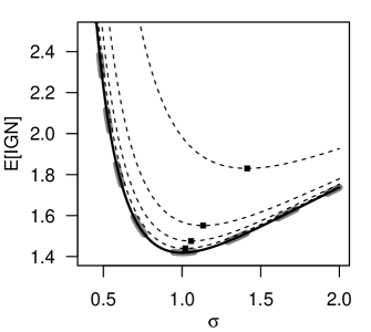
Figure 2: Verifications $x$ are drawn iid from $\mathcal{N}(0,1)$, and $m$-member ensembles are drawn iid from $\mathcal{N}(0,\sigma^{2})$. The dashed gray line corresponds to the expected Ignorance score for $m\rightarrow\infty$, the black dashed lines correspond to the expected standard Ignorance scores of finite ensembles (from top to bottom: $m=5,10,20,50$), and the black full line shows the expected bias-corrected Ignorance score (independent of $m$). Markers indicate the minima along their respective curves.

Figure 2 illustrates differences between the standard and bias-corrected Ignorance score if ensembles and observations are drawn from different distributions (unlike Figure 1). Artificial observations are drawn again iid from $\mathcal{N}(0,1)$, and artificial $m$-member ensembles are drawn iid from $\mathcal{N}(0,\sigma^{2})$. The expectations of the standard Ignorance score, of the population Ignorance score, and of the bias-corrected Ignorance score, taken over the distributions of the observations and ensembles, are shown as functions of $\sigma$. Note that these expectations could also be approximated by sample averages over large data sets of forecasts and observations drawn from the respective distributions. The systematic bias due to the finiteness of the ensemble shows as a vertical offset of the curves. The vertical offset is the larger, the smaller the ensemble is, and at any given value of $\sigma$, the expected standard Ignorance score can be improved by generating a larger ensemble. In contrast to the standard Ignorance score, the expectation (or long-term average) of the bias-corrected Ignorance score is equal to the expected population Ignorance score for all values of $\sigma$ and $m$.

Figure 2 further shows that the standard Ignorance score rewards ensembles that violate statistical consistency (Anderson, 1996) (i.e., the statistical indistinguishability between ensemble members and observations). The expected standard Ignorance score obtains its optimum at a value of $\sigma$ which differs from the standard deviation of the observation. The standard Ignorance score therefore rewards ensemble forecasts that have different statistical properties than the observation. The ensemble that optimizes the expected standard Ignorance score is overdispersive, that is its spread is on average higher than that of the observation. The ensemble forecasts that minimise the expected standard Ignorance score would therefore not pass the test for statistical consistency proposed by Anderson (1996), and the individual ensemble members cannot be interpreted as equally likely scenarios for the observation.

The expectation of the bias-corrected Ignorance score $\mathcal{I}^{*}$ is equal to the population Ignorance score. The equality holds for all ensemble sizes greater than 3. Increasing the ensemble size, say from 5 to 10, does not improve the expected value of $\mathcal{I}^{*}$. As a consequence of unbiasedness with respect to the ensemble size, the score $\mathcal{I}^{*}$ does not suffer from the bias of the optimum. The expectation of $\mathcal{I}^{*}$ is optimized if the ensemble members are drawn from the same distribution as the observation. Ensembles are rewarded for being statistically consistent with the observation.

The expectation of the estimator $\mathcal{I}^{*}$ is insensitive to the number of ensemble members. It can therefore be used to compare ensembles of different sizes. But $\mathcal{I}^{*}$ also estimates the potential Ignorance score of an infinitely large ensemble. There might be cases where a $m$-member ensemble is available, but the forecaster is interested in the potential score if the ensemble had $M\neq m$ members. For example, he might be interested in the number of members he would have to generate in order to achieve a certain Ignorance score, or whether his $m$-member ensemble forecasting system would outperform a competing $M$-member ensemble if it had the same number of members. In appendix A.4, we have derived an estimator of the Ignorance score, denoted $\mathcal{I}^{*}_{m\rightarrow M}$ (Eq. (30)), which extrapolates the Ignorance score of an $m$-member ensemble to the score that it would achieve if it had $M\neq m$ members. The score $\mathcal{I}^{*}_{m\rightarrow M}$ is included for completeness, and will not be discussed further in this article.

3 Application to seasonal climate prediction

Figure 3: Upper panel: Time series of System4 ensemble forecasts (small gray markers) and observations (large black markers) for surface air temperature averaged over the gray area in the lower left panel. Lower right panel: P-values of Shapiro-Wilk normality tests applied to the individual ensemble forecasts, plotted over time.

We illustrate the possible benefits of using a bias-corrected score by a practical example. We consider ensemble predictions of the summer (JJA) mean air surface temperature over land over the area limited by 30N – 75N and 12.5W – 42.5E, initialized on the 1 May of the same year. The forecasts are generated by ECMWF’s seasonal forecast system “System4” (Molteni et al., 2011) with start dates from 1981 to 2010 ($n=30$), and $m=51$ ensemble members. Verifying observations are taken from the WFDEI gridded data set (Weedon et al., 2011; Dee et al., 2011). All data were downloaded through the ECOMS user data gateway (ECOMS User Data Gateway, 2014). The ensemble and observation time series are plotted in Figure 3, along with the geographical region over which temperatures have been averaged. Visual inspection shows that a Normal approximation of the ensemble forecasts is justified, which is strengthened by the approximately uniform distribution of the p-values of Shapiro-Wilk normality tests applied to the ensembles. The System4 ensemble has a cold bias of $\approx-0.3K$. The observations show a linear trend of $\approx 0.05K/yr$ which is reasonably well reproduced by the ensemble mean ($\approx 0.03K/yr$). After removing linear trends, the Pearson correlation coefficient between ensemble means and observations is $0.46$.

We study the effects of finite ensemble sizes by sampling smaller subensembles from the full 51-member ensemble and calculate their Ignorance scores. At each time $t=1,\cdots,30$ we randomly sample $\tilde{m}\leq m$ ensemble members without replacement, and calculate the Ignorance score (averaged over all $t$), using the estimators $\widehat{\mathcal{I}}$ and $\mathcal{I}^{*}$. At each value of $\tilde{m}$, scores are averaged over $10^{3}$ realizations of random subensembles.

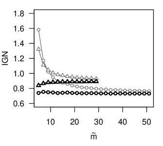
Figure 4: Illustration of the effect of finite ensemble sizes on the average Ignorance score, comparing climatological ensembles of size $\tilde{m}$ (triangles) to System4 ensembles of size $\tilde{m}$ (circles). The standard Ignorance score $\widehat{\mathcal{I}}$ is shown in gray, and the bias-corrected Ignorance score $\mathcal{I}^{*}$ is shown in black.

In Figure 4, the average standard Ignorance score and average bias-corrected Ignorance score of the $\tilde{m}$-member System4 ensembles are compared to the scores of $\tilde{m}$-member climatological ensembles. These are randomly sampled without replacement from the 30 years of observation data. In order to avoid spurious skill, a climatological ensemble for time $t$ never includes the observation at time $t$; the maximum value of $\tilde{m}$ for the climatological ensemble is therefore 29. Figure 4 shows that the average standard Ignorance score $\widehat{\mathcal{I}}$ depends systematically on the number of ensemble members, while the average bias-corrected Ignorance score $\mathcal{I}^{*}$ is insensitive to the ensemble size, except for a slight trend at small values of $\tilde{m}$. The dependence of $\widehat{\mathcal{I}}$ on the ensemble size leads to the conclusion that a 29-member climatological ensemble is preferable to a 10 member System4 ensemble. For very small ensemble sizes, the climatological ensemble has a lower standard Ignorance score than the System4 ensemble, even if the number of members is equal. This difference might be due to the cold bias of the System4 ensemble. The above remarks highlight the important difference between the two scores: While the standard Ignorance score evaluates the forecast that was derived from a finite ensemble, the bias-corrected Ignorance score evaluates the underlying distribution from which the finite ensemble was drawn. The sensitivity to ensemble size of the score that evaluates the derived forecast can lead to the conclusion that forecasts derived from a large ensemble generated by a simple forecasting system such as climatology is superior to a small ensemble generated by a sophisticated physical-dynamical forecasting system. Larger ensembles allow for more robust estimation of the forecast distribution, which is reflected by the finite-ensemble bias of the standard Ignorance score. On the other hand, the underlying distribution is independent of the ensemble size. If the bias-corrected Ignorance score is used to evaluate this underlying distribution, the more sophisticated System4 always outperforms the climatological ensemble in this score, independent of the number of ensemble members. This result suggests that the underlying (time-varying) distributions from which System4 samples its ensembles assign, on average, higher probability to the observations than the (time-constant) climatological distribution.

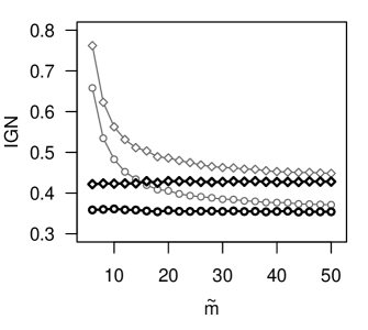
Figure 5: Illustration of the effect of finite ensemble sizes on the average Ignorance score, comparing unbiased ensembles of size $\tilde{m}$ (circles) to artificially biased ensembles of size $\tilde{m}$ (diamonds). The standard Ignorance score $\widehat{\mathcal{I}}$ is shown in gray, and the bias-corrected Ignorance score $\mathcal{I}^{*}$ is shown in black.

For the next analysis we create artificial ensembles whose underlying distributions vary in time, but which are (with great certainty) not more skilful than System4. We first transform System4 ensemble and observation data to anomalies by removing their respective grand averages. We then create a biased version of System4 by adding to each forecast an artificial bias of 0.25 climatological standard deviations ($\approx 0.15K$). We assume that a verification measure that evaluates the underlying distribution should be expected to rank the unbiased System4 ensemble better than the artificially biased System4 ensemble, independent of ensemble size. In Figure 5 we compare the unbiased System4 ensemble with the artificially biased System4 ensemble at different values of $\tilde{m}$, using the standard estimator and bias-corrected estimator of the Ignorance score. Figure 5 shows that the standard Ignorance $\widehat{\mathcal{I}}$ on average assigns a better score to a biased ensemble with more than $20$ members than to an unbiased ensemble with less than $10$ members. On the other hand, the bias-corrected Ignorance score always ranks the two ensemble forecasts such that the unbiased ensembles obtains a better average score than the biased ensembles, independent of the number of members. This analysis shows that, forecast distributions derived from a biased ensemble can achieve better average scores than forecast distributions derived from unbiased ensembles if the biased ensemble has more members. The more robust estimation of the forecast distribution from a larger ensemble offsets the disadvantage due to the systematic bias. On the other hand, if the bias-corrected Ignorance score is used to evaluate the underlying distributions of the ensembles, the average score of an inferior (e.g. biased) ensemble cannot be improved simply by adding more members.

The resampling approach of this section can be used as an alternative method to estimating the finite-ensemble effect of a verification score. By subsampling the larger ensemble down to the size of the smaller ensemble, and averaging over many realizations of the subsampling, we can approximate the standard Ignorance score that the larger ensemble would achieve if it had less members. This makes the average standard Ignorance scores of two competing ensembles comparable at the smaller ensemble size. This alternative approach to accounting for the finite-ensemble bias deserves further attention, but will not be studied here in more detail. We only note that subsampling and averaging is computationally more expensive than calculating a bias-corrected score that accounts for the finite-ensemble effect by its mathematical properties. Furthermore, the subsampling approach cannot be used to estimate the score that an ensemble would achieve if it had more members.

4 Discussion

4.1 The underlying distribution and derived forecasts

By correcting the finite-ensemble bias of the standard Ignorance score, we have derived an unbiased estimator of the score of the underlying distribution. Deriving a score whose expectation is independent of the ensemble size seems irreproachable, and has been achieved for different scores (cf. references in section 1). But the concept of evaluating the unknown underlying distribution warrants further discussion. In this section, we argue that a clear distinction must be made between an evaluation of a derived forecast distribution, which depends on ensemble size, and an evaluation of the underlying distribution, which should be independent of ensemble size.

The underlying distribution is a hypothetical concept. The individual ensemble members are perceived as random quantities and this randomness is described by an underlying distribution. Ensemble forecasting systems can be imagined as (high-dimensional) random number generators that draw samples from the underlying distribution. The underlying distribution can therefore be thought of as a part of the ensemble forecasting system. Estimating the score of the underlying distribution can therefore be interpreted as a quantification of the skill of the ensemble forecasting system. Evaluating the score of the underlying distribution is therefore especially relevant for model developers, who are interested in the quality of the forecasting system.

Even though we can retrospectively estimate its score, the underlying distribution is not accessible for forecasting. Only finite ensembles drawn from that distribution are ever available and the number of members is limited by the computational resources. Forecasters and decision-makers have to rely on probabilistic forecasts derived from the finite ensemble. These forecast users will probably be more interested in an estimate of the score of the derived forecast than in an estimate of the score of the underlying distribution. For these users, the finite-ensemble bias is a practically relevant effect – more ensemble members allow for a more robust estimation of the forecast distribution, and it is sensible to assume that larger ensembles provide better forecasts. However, the same user might also be interested in statistically consistent ensemble forecasts, for example if individual members of a global forecast model are used as scenarios to drive a high-resolution regional model. In that case, rewarding ensembles for being statistically consistent by using a bias-corrected score might be preferable.

We have shown that, due to the finite-ensemble bias, the average Ignorance score of the derived forecast is not necessarily indicative of the average Ignorance score of the underlying distribution. Due to the finite-ensemble bias, it is possible that a forecast derived from a statistically inconsistent, biased, or simple climatological forecast system outperforms forecasts derived from statistically consistent, unbiased, or sophisticated physical-dynamical ensemble forecasts. If the underlying distribution were available, the latter forecasts might be preferable to the former. But the difference in ensemble size, and the fact that derived forecasts from finite ensembles are evaluated, reverses the preference.

4.2 When is the finite-ensemble bias-correction desired?

There are situations, where the bias-correction is clearly not desired, namely when the quality of the derived probability forecast is of interest, instead of the quality of the underlying ensemble distribution. If a probability forecast is always generated using a specified number of ensemble members, and a Normal approximation $\mathcal{N}(\hat{\mu},\hat{\sigma}^{2})$ is used, the standard Ignorance score $\widehat{\mathcal{I}}$ rather than the bias-corrected Ignorance score $\mathcal{I}^{*}$ is the correct version of the Ignorance score to evaluate this probability forecast. The potential score for $m\rightarrow\infty$ is of no interest in this case, because only finitely many ensemble members are ever available. The bias of the optimum is acceptable if it implies that a statistically inconsistent ensemble provides a better probability forecast than a statistically consistent one. However, due to the bias of the optimum, the members of the optimal ensemble are not necessarily exchangeable with the observation. The individual members must therefore not be interpreted as “possible future scenarios”. In fact, the individual ensemble members should not be interpreted at all in this case; only the derived continuous forecast distribution is of interest.

There are at least three applications where an estimation or correction of the finite-ensemble bias is clearly desirable: Firstly, in numerical model development, often new ensemble prediction systems are to be explored, using for example a new initialization technique, a new parametrization scheme, or an experimental dynamical core. If we adopt the notion that the hypothetical underlying distribution is a property of the forecasting system, such modifications of the forecasting system change, and possibly improve, the score of the underlying distribution. In such pilot studies, it might be desirable to limit CPU time by generating ensembles with fewer members than the final (operational) forecast product will have, and then accounting for the finite ensemble bias by using a suitable score. Estimating the score of the underlying distribution then provides a more realistic estimate of the score of the final product, especially in relation to competing forecasting systems with possibly larger ensembles.

Secondly, if ensembles of different sizes are compared and forecasts derived from them have different scores, it might be of interest whether the larger ensemble achieves a better score due to the finite-ensemble bias, or because its underlying distribution is more skilful at predicting the real world and therefore assigns higher probablity to the observations. This difference is illustrated in section 3, where it is shown that a biased ensemble can outperform an unbiased ensemble merely by having more members. A score that accounts for the finite-ensemble bias can be used to inform the forecaster that increasing the size of the smaller ensemble to the size of the bigger ensemble could produce an even better forecast.

Lastly, the bias of the optimum of the standard Ignorance score, illustrated in Figure 2, is clearly undesirable when the Ignorance score is used as an objective function for parameter estimation and optimization. For example, a verification score might be used to tune parameters of the ensemble forecasting system to match as well as possible the corresponding parameter of the observation (such as the standard deviation in Figure 2). A biased score which evaluates the derived forecast distribution might favor an ensemble that differs systematically from the observations. Even though the ensemble system optimized by the biased score has been tuned to generate the best possible forecasts, the ensemble members do not behave like the real world. Removing the bias of the optimum by using a bias-corrected score ensures that the optimised ensemble is statistically consistent with the observations. The optimised parameter values of the ensemble are equal to the parameter values of the real world (provided the parameter really has a physical interpretation). Additionally, the optimal value of the parameter does not change if the ensemble size is changed. If the score that is used for parameter tuning has a bias of the optimum, the parameters would have to be re-tuned whenever the ensemble size is changed. We consider unbiased parameter estimation and optimisation a relevant and promising application of bias-corrected verification scores, but more work is necessary to fully explore their applicability and limitations.

4.3 Propriety and fairness

A scoring rule $S$ is proper (relative to a class $\mathcal{P}$ of probability measures) if, for any $q\in\mathcal{P}$, the expected score taken over the distribution $q$ of the observation $x$, $\mathds{E}_{x\sim q}[S(p,x)]$, is optimized when $p=q$ (Gneiting and Raftery, 2007). A proper scoring rule thus favours (on average) forecasts $p$ that equal the distribution $q$ of the observation. The standard Ignorance score defined by Eq. (1) is a proper scoring rule. Here, $S$ is a function of an observation $x$ and a distribution $p$. Our forecast is an ensemble, not a distribution, so we must decide what distribution to use for $p$. If we use a distribution derived from the ensemble, such as $\mathcal{N}(\hat{\mu},\hat{\sigma}^{2})$, then the standard Ignorance score favours (on average) ensembles for which the derived distribution $\mathcal{N}(\hat{\mu},\hat{\sigma}^{2})$ equals the distribution of the observation. If we want to evaluate the derived distribution as a probability forecast then the standard Ignorance score is a proper score to use. But we have shown that ensembles that optimise the standard Ignorance score on average are not those whose underlying distribution equals the distribution of the observation.

Recently, Fricker et al. (2013) and Ferro (2013) introduced fair scores as a possible extension of proper scores to ensemble forecasts. If we want to evaluate the underlying distribution, and thereby favour ensembles whose underlying distribution equals the distribution of the observation (so that ensembles and observations are statistically consistent, for example) then we should use a fair score. A scoring rule $S^{*}$ is fair (relative to a class $\mathcal{P}$ of probability measures) if, for any $p,q\in\mathcal{P}$, the expectation of the score, taken with respect to the distribution $q$ of the observation $x$, and with respect to the distribution $p$ from which the ensemble members $y_{i}$ were independently drawn, $\mathds{E}_{x\sim q}\mathds{E}_{y_{i}\sim p}[S^{*}(y,x)]$, is optimized when $p=q$. A fair score thus favours (on average) ensembles whose underlying distribution is equal to the distribution of the observation. The bias-corrected Ignorance score is fair relative to the class of Normal distributions. Here, $S^{*}$ is a function of an observation $x$ and an ensemble $y$. Since $y$ is not a distribution, it would not be meaningful to ask whether $\mathcal{I}^{*}$ is proper. It is true, however, that $S(p,x):=\mathds{E}_{y_{i}\sim p}[S^{*}(y,x)]$ is proper. The reader is referred to Ferro (2013) for more discussion of the relation between fair and proper scores.

Unbiasedness of the bias-corrected Ignorance $\mathcal{I}^{*}$ only holds for independent and identically Normal distributed ensemble members. If the ensemble members are non-Normal, $\mathcal{I}^{*}$ is biased (cf. section 4.4 and appendix B). Therefore, (adopting the terminology of Gneiting and Raftery (2007)), we say that the score $\mathcal{I}^{*}$ is fair relative to the class of Normal distributions. In contrast, the fair continuous ranked probability score (fair CRPS) for continuous ensemble forecasts proposed by Fricker et al. (2013) is independent of the distribution of the ensemble members, and therefore has wider applicability than the fair Ignorance score presented here. Note that there is an interesting difference between the Ignorance score and the CRPS. According to Figure 2, the standard Ignorance score favors overdispersive ensemble forecasts. By contrast, according to Figure 2 of Ferro (2013), the CRPS without fairness adjustment favors underdispersive ensembles. This difference shows that without a bias-correction for finite ensemble sizes, different proper scores can favor ensembles that are not only inconsistent with the observation, but the nature of the inconsistency can also be fundamentally different for different scores. This is shown by the bias of the optimum of the standard deviation, which is positive for the standard Ignorance score and negative for the unadjusted CRPS.

4.4 Non-Normal data

We have shown in section 2 that the bias-corrected Ignorance score $\mathcal{I}^{*}$ completely removes the finite-ensemble bias if the ensemble members are identically and independently Normal distributed. In practical applications such as atmospheric forecasts, where ensemble members are generated by complex numerical computer simulations, Normality appears to be too strong an assumption. It is unrealistic to assume that outputs from computer simulations are exactly Normally distributed. However, if the ensemble members are not iid Normal distributed, a basic assumption in the derivation of $\mathcal{I}^{*}$ is violated, and $\mathcal{I}^{*}$ might be biased after all.

We show in appendix B that for non-Normal ensemble members, $\mathcal{I}^{*}$ is indeed biased. This is shown for ensembles with heavy-tailed distributions, skewed distributions and bimodal distributions. But the bias of $\mathcal{I}^{*}$ is always considerably smaller than the bias of $\widehat{\mathcal{I}}$. This reduction of the finite-ensemble bias implies that if the ensemble data suggests a Normal approximation, and if the finite-ensemble bias of the Ignorance score is undesired, $\mathcal{I}^{*}$ should be used for ensemble verification, rather than $\widehat{\mathcal{I}}$.

4.5 Bias-variance decomposition

Bias is not the only factor that contributes to differences between a finite sample estimator and the corresponding population value. Another important factor is the estimator variance, i.e. the average squared difference of the estimator from its expectation. The sum of the squared bias and the variance can be shown to be equal to the expected squared error of the estimator, i.e. the expected squared difference between the estimator and the population value (Mood, 1950, sec. 7.3). That is, an unbiased estimator can still have a larger error than a biased estimator, by having a very large variance. This is not the case for $\mathcal{I}^{*}$. We show in appendix A.3, that under a first order approximation, the conditional variance of $\mathcal{I}^{*}(\hat{\mu},\hat{\sigma}^{2};x)$, given $x$, is always smaller than the conditional variance of $\widehat{\mathcal{I}}$. This means, that $\mathcal{I}^{*}$ is not only equal to the population score on average, it is also on average closer to the population score in a mean-squared sense, which provides further motivation to use $\mathcal{I}^{*}$ instead of $\widehat{\mathcal{I}}$.

5 Summary and outlook

We have studied the applicability of the Ignorance score for ensemble verification. We focused on Normal approximations, where the ensemble forecast is transformed to a continuous Normal forecast distribution whose parameters are estimated by the ensemble mean and variance. It was shown that the Ignorance score applied to this forecast distribution is biased with respect to the ensemble size: Larger ensembles obtain systematically better scores. In section 2 a new estimator of the Ignorance score was derived which removes the finite ensemble bias; the expectation of the new estimator is independent of the number of ensemble members. The main advantage of the new score is that it allows for a fair comparison of ensemble forecasts with different number of members. This was illustrated in section 3 by application to seasonal climate forecasts. It was shown that the standard Ignorance score favors biased or climatological ensembles with many members over unbiased and physical dynamical ensembles with few members. In contrast, the bias-corrected Ignorance score on average ranks the statistically consistent and physical dynamical ensemble better, regardless of the number of members. In section 4, we concluded that the bias-corrected Ignorance score is applicable also to non-Normal ensemble data, and that the new score estimator not only reduces the bias, but also the estimator variance, thereby decreasing the overall estimation error of the score. It was shown that the new estimator is a strictly fair score, and situations were discussed when bias-corrected scores are preferable for ensemble evaluation.

There is some scope to extend the results of this paper. For example, it might be possible to derive a bias-corrected Ignorance score of a multivariate Normal forecast, since the sampling distributions of the multivariate sample mean and covariance matrix are known. Further, a bias-corrected score for affine transformations of ensemble forecasts would be useful to assess the quality of ensemble forecasts that were recalibrated by such a transformation. However, affine transformations can introduce correlations between the ensemble members, and deriving a bias-corrected score for non-independent ensembles is difficult. It might also be possible to derive bias-corrected estimators of different verification scores under a Normal assumption, or bias-corrected estimators of the Ignorance under different distributions. This paper provides a framework for how these problems can be approached, and how the properties of the resulting estimators can be analysed.

The results of this article are potentially useful outside the area of forecast verification. First of all, the Ignorance score can be regarded as the negative log-likelihood of a Normal distribution which is represented by a finite sample. The bias correction derived in section 2 might be useful for maximum likelihood parameter estimation. Furthermore, the Ignorance score is motivated by the entropy as an information-theoretic measure of predictability (Roulston and Smith, 2002). The bias-corrected version derived in this article might therefore be useful to account for finite-ensemble effects in information-theoretic predictability frameworks (DelSole and Tippett, 2007).

Appendix A Appendix: Proofs

A.1 $\mathds{E}[\log\hat{\sigma}]$

The derivation follows from the properties of distributions in the exponential family and their sufficient statistics (Lehmann and Casella, 1998, sec. 1.5). If $X\sim\chi^{2}_{m-1}$, we can define $\tau:=(m-1)/2-1$ and write the pdf of $X$ as

$$p_{X}(x)=\exp\left\{\tau\log x-\frac{x}{2}-(\tau+1)\log 2-\log\Gamma(\tau+1)\right\}.$$ (14)

Differentiating the integral $\int dx\ p_{X}(x)$ with respect to $\tau$ yields

$$\mathds{E}[\log X]=\log 2+\Psi\left(\frac{m-1}{2}\right)$$ (15)

where $\Psi(x)=d/dx\log\Gamma(x)$ is the digamma function. Applying Eq. (15) to $\hat{\sigma}^{2}$, whose distribution is given by Eq. (8), we get

$$\mathds{E}\left[\log\hat{\sigma}^{2}\right]= \mathds{E}\left[\log\frac{m-1}{\sigma^{2}}\hat{\sigma}^{2}\right]+\log\frac{\sigma^{2}}{m-1}$$ (16)

$$= \log\sigma^{2}+\Psi\left(\frac{m-1}{2}\right)-\log\left(\frac{m-1}{2}\right).$$ (17)

A.2 $\mathds{E}\left[\left(\frac{\hat{\mu}-x}{\hat{\sigma}}\right)^{2}\right]$

Let the independent random variables $Z$ and $V$ have distributions $Z\sim\mathcal{N}(0,1)$ and $V\sim\chi^{2}_{m-1}$. Then the non-central t-distribution $t_{m-1,x}$, with $m-1$ degrees of freedom and noncentrality parameter $x$, is defined through

$$\frac{Z+x}{\sqrt{V/(m-1)}}\sim t_{m-1,x}$$ (18)

Using the sampling distributions of $\hat{\mu}$ and $\hat{\sigma}^{2}$, and their independence, we get the following relation:

$$\sqrt{m}\frac{\hat{\mu}-x}{\hat{\sigma}}= \frac{\frac{\hat{\mu}-\mu}{\sigma/\sqrt{m}}+\frac{\sqrt{m}}{\sigma}(\mu-x)}{\sqrt{\frac{m-1}{\sigma^{2}}\hat{\sigma}^{2}}/\sqrt{m-1}}$$ (19)

$$\sim\ t_{m-1,\frac{\sqrt{m}}{\sigma}(\mu-x)}.$$ (20)

The raw moments of a random variable $T\sim t_{m,x}$ are given by Hogben et al. (1961):

$$\mathds{E}\left[T^{k}\right]=\left(\frac{m}{2}\right)^{\frac{k}{2}}\frac{\Gamma\left(\frac{m-k}{2}\right)}{\Gamma\left(\frac{m}{2}\right)}\exp\left(-\frac{x^{2}}{2}\right)\frac{\partial^{k}}{\partial x^{k}}\exp\left(\frac{x^{2}}{2}\right).$$ (21)

By calculating the second raw moment of $\sqrt{m}(\hat{\mu}-x)/\hat{\sigma}$ and dividing by $m$ we get

$$\mathds{E}\left[\left(\frac{\hat{\mu}-x}{\hat{\sigma}}\right)^{2}\right]=\frac{m-1}{m-3}\left(\frac{\mu-x}{\sigma}\right)^{2}+\frac{m-1}{m(m-3)}.$$ (22)

A.3 $var(\mathcal{I}^{*})\leq var(\widehat{\mathcal{I}})$

In this appendix, we calculate approximate expressions for the variances of the standard and bias-corrected Ignorance score. To be more precise, we calculate the conditional variance of $\mathcal{I}(\hat{\mu},\hat{\sigma}^{2};x)$, given $x$. Only variability of the random variables $\hat{\mu}$ and $\hat{\sigma}^{2}$ contributes to the variance, while the observation $x$ is kept constant. The results are used to show that $var(\mathcal{I}^{*})\leq var(\widehat{\mathcal{I}})$.

It follows from the sampling distributions of $\hat{\mu}$ and $\hat{\sigma}^{2}$ (Eq. (7) and Eq. (8)) that $var(\hat{\mu})=\sigma^{2}/m$ and $var(\hat{\sigma}^{2})=2\sigma^{4}/(m-1)$. Furthermore, $\hat{\mu}$ and $\hat{\sigma}^{2}$ are statistically independent. We use these results to approximate the variance of $\widehat{\mathcal{I}}$ by propagation of error (Mood, 1950, sec. 2.3). A first-order Taylor expansion of $\widehat{\mathcal{I}}(\hat{\mu},\hat{\sigma}^{2};x)$ around $\mu$ and $\sigma^{2}$ yields

$$var[\widehat{\mathcal{I}}(\hat{\mu},\hat{\sigma}^{2};x)]\approx\left(\frac{\partial\widehat{\mathcal{I}}}{\partial\hat{\mu}}\right)^{2}var(\hat{\mu})+\left(\frac{\partial\widehat{\mathcal{I}}}{\partial\hat{\sigma}^{2}}\right)^{2}var(\hat{\sigma}^{2})$$ (23)

and analogously for $\mathcal{I}^{*}$. Define the variable $\hat{z}=(\hat{\mu}-x)/\hat{\sigma}$. Then the approximate variances of $\widehat{\mathcal{I}}$ and $\mathcal{I}^{*}$ are given by

$$var(\widehat{\mathcal{I}}) \approx\frac{\hat{z}^{2}}{m}+\frac{1}{2(m-1)}\left(1-\hat{z}^{2}\right)^{2}\text{, and}$$ (24)

$$var(\mathcal{I}^{*}) \approx\left(\frac{m-3}{m-1}\right)^{2}\frac{\hat{z}^{2}}{m}+\frac{1}{2(m-1)}\left(1-\frac{m-3}{m-1}\hat{z}^{2}\right)^{2}$$ (25)

It follows from Eq. (24) and Eq. (25) that the difference between the variances is

$$var(\widehat{\mathcal{I}})-var(\mathcal{I}^{*})=\frac{2\hat{z}^{4}}{(m-1)^{2}}\left(1-\frac{1}{m-1}\right)+\frac{2\hat{z}^{2}}{m(m-1)^{2}}(m-4)$$ (26)

which is non-negative for all $m\geq 4$. That is, under the first-order approximation, the conditional variance of $\mathcal{I}^{*}$, given $x$, is never greater than the conditional variance of $\widehat{\mathcal{I}}$. The result is independent of the value of the observation $x$.

A.4 $\mathcal{I}^{*}_{m\rightarrow M}$

We write the ensemble mean and variance calculated from an $m$-member ensemble by $\hat{\mu}_{m}$ and $\hat{\sigma}^{2}_{m}$, respectively. In this appendix we show how to use $\hat{\mu}_{m}$ and $\hat{\sigma}^{2}_{m}$ to estimate the Ignorance score that the same ensemble would achieve if it had $M\neq m$ members. First note that it follows from Eq. (9) that

$$\mathds{E}\left[\log\hat{\sigma}^{2}_{M}\right]=\mathds{E}\Bigg{[} \log\hat{\sigma}^{2}_{m}-\Psi\left(\frac{m-1}{2}\right)+\Psi\left(\frac{M-1}{2}\right)+$$

$$\log\left(\frac{m-1}{2}\right)-\log\left(\frac{M-1}{2}\right)\Bigg{]},$$ (27)

where $\hat{\sigma}^{2}_{m}$ and $\hat{\sigma}^{2}_{M}$ are ensemble variances of $m$- and $M$-member ensembles sampled from the same distribution. Similarly, it follows from Eq. (10) that

$$\mathds{E}\left[\frac{(\hat{\mu}_{M}-x)^{2}}{\hat{\sigma}^{2}_{M}}\right]=\mathds{E}\Bigg{[} \left\{\left(\frac{m-3}{m-1}\right)\frac{(\hat{\mu}_{m}-x)^{2}}{\hat{\sigma}^{2}_{m}}-\frac{1}{m}\right\}\frac{M-1}{M-3}+$$

$$\frac{M-1}{M(M-3)}\Bigg{]},$$ (28)

where $\hat{\mu}_{m}$ and $\hat{\mu}_{M}$ are ensemble means of $m$- and $M$-member ensembles sampled from the same distribution. Using Eq. (27) and Eq. (28), we can derive the score

$$\mathcal{I}^{*}_{m\rightarrow M}(\hat{\mu}_{m},\hat{\sigma}^{2}_{m};x)$$ (29)

$$=\frac{1}{2}\log 2\pi+\frac{1}{2}\log\hat{\sigma}^{2}_{m}+\frac{1}{2}\left(\frac{M-1}{M-3}\right)\left(\frac{m-3}{m-1}\right)\frac{(\hat{\mu}_{m}-x)^{2}}{\hat{\sigma}^{2}_{m}}$$

$$+\frac{1}{2}\left[\Psi\left(\frac{M-1}{2}\right)-\Psi\left(\frac{m-1}{2}\right)\right.$$

$$+\log\left(\frac{m-1}{M-1}\right)+\left.\frac{(m-M)(M-1)}{Mm(M-3)}\right],$$ (30)

which satisfies

$$\mathds{E}\Big{[}\mathcal{I}^{*}_{m\rightarrow M}(\hat{\mu}_{m},\hat{\sigma}^{2}_{m};x)\Big{]}=\mathds{E}\Big{[}\widehat{\mathcal{I}}(\hat{\mu}_{M},\hat{\sigma}^{2}_{M};x)\Big{]}.$$ (31)

That is, the score $\mathcal{I}^{*}_{m\rightarrow M}$ is a function of the sample mean and variance of an $m$-member ensemble, but on average it is equal to the Ignorance score of a hypothetical $M$-member ensemble sampled from the same distribution.

Appendix B Appendix: Behavior for Non-Normal ensemble data

In this appendix, we consider the effect of non-Normal ensemble data on the bias of the Ignorance score. If the ensemble members are not iid Normal distributed, an additional systematic error arises. By making the Normal assumption for non-Normal ensembles, possible features of the forecast distribution such as heavy-tailedness, skewness, or multimodality are neglected. Suppose the observation is a skewed random variable, and the ensemble is indeed drawn from the correct skewed distribution. Transforming the ensemble to a Normal distribution degrades the skill of the ensemble forecasting system, because skewness is ignored. In this case, the average Ignorance score of the Normal approximation of the forecast distribution is worse than the average Ignorance score that the true ensemble distribution would achieve, if it were known. Clearly, the ensuing bias due to non-Normality of the ensemble is not removed by $\mathcal{I}^{*}$.

For ensemble forecasts which are obviously non-Normal, i.e. which have members that are gross outliers, which are heavily skewed or which exhibit strong multimodality, a Normal assumption would not be made in practice. The Ignorance score should not be estimated by Eq. (5) for these ensembles, and a bias-corrected Ignorance score for Normal ensembles is of no interest in such cases.

On the other hand, there might be a moderate violation of Normality, which is not immediately obvious, or which is small enough such that a Normal assumption seems a good approximation. In this section, we consider three kinds of moderate deviations from Normality that might occur in practical applications: Heavy-tailedness, skewness, and bimodality. In order to keep things simple, we consider only reliable ensembles which are always drawn from the same distribution as their verifying observation. Furthermore, all distributions are scaled and shifted to have zero mean and unit variance. In each case, the degree of Normality is tuned by a distribution-specific Normality parameter $\theta$, that has a limiting value for which the respective distribution converges to the standard Normal distribution.

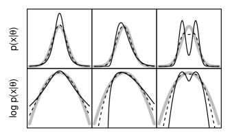
Figure 6: Illustration of the types of Non-Normality considered. Left column: Heavy-tailed t-distributions with $\theta=4$ ( ) and $\theta=20$ (   ) degrees of freedom. Middle column: Positively skewed Gamma distributions with shape parameter $\theta=5$ ( ) and $\theta=50$ (   ). Right column: Bimodal Normal mixture with modes at $\theta=\pm 0.9$ ( ) and $\theta=\pm 0.75$ (   ). All distributions have been scaled and shifted to have zero mean and unit variance. The standard Normal distribution is shown in gray.

We simulate heavy-tailed ensembles and observations by Student’s t-distribution, denoted by $t_{\theta}$. The parameter $\theta$ (which we assume to be $>2$) denotes the degree of freedom of the t-distribution. The t-distribution has zero mean and converges to the Normal distribution for $\theta\rightarrow\infty$. The random variable $X\sim t_{\theta}$ has variance $\theta/(\theta-2)$. Thus, the random variable $\sqrt{(\theta-2)/\theta}X$ has unit variance, as desired for our study. Secondly, we simulate skewed ensembles and observations by a Gamma distribution $\Gamma(\theta,\sqrt{\theta})$ with shape parameter $\theta$. By setting the rate parameter to $\sqrt{\theta}$ the variance is set to unity. The random variable $X\sim\Gamma(\theta,\sqrt{\theta})$ has mean equal to $\sqrt{\theta}$, thus the random variable $X-\sqrt{\theta}$ has zero mean. The Gamma distribution $\Gamma(\theta,\sqrt{\theta})$ has skewness $2/\sqrt{\theta}$ and converges to the Normal distribution for $\theta\rightarrow\infty$. Lastly, we simulate bimodal ensembles and observations by a Normal mixture. Define the Bernoulli-distributed random variable $U\sim Ber(1/2)$ and the Normal random variable $Y\sim\mathcal{N}(\theta,1-\theta^{2})$. Then the random variable $X=(2U-1)Y$ has a bimodal Normal distribution with modes at $\pm\theta$, zero mean, and unit variance. The parameter $\theta\in[0,1)$ tunes the Normality; for $\theta=0$ the distribution of $X$ is the standard Normal. The three types of non-Normal distributions are sketched in Figure 6 for different values of $\theta$.

For observations and ensembles sampled from a Nonnormal distribution with some parameter $\theta$, we calculate 4 different Ignorance scores:

1. The population Ignorance score of the underlying distribution $p(x|\theta)$ from which the observation was sampled, denoted by $\mathcal{I}_{p}:=-\log p(x|\theta)$.

2. The Ignorance score of the Normal approximation of $p(x|\theta)$, denoted by $\mathcal{I}_{n}$. Recall that all non-Normal distributions that we consider always have zero mean and unit variance; the standard Normal is therefore always the best Normal approximation of the true $p(x|\theta)$, and we have $\mathcal{I}_{n}(x)=\log(2\pi)^{-1/2}+x^{2}/2$ every time.

3. The standard Ignorance score $\widehat{\mathcal{I}}$, calculated by Eq. (5), using the ensemble mean and ensemble standard deviation; and

4. The bias-corrected Ignorance score $\mathcal{I}^{*}$, calculated by Eq. (12), where we also use the ensemble mean and ensemble standard deviation.

Note that $\mathcal{I}_{p}$ and $\mathcal{I}_{n}$ are independent of any ensemble forecast.

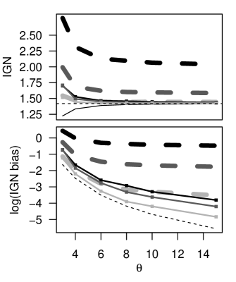
Figure 7: Ignorance scores and their biases for heavy-tailed data as functions of the non-Normality parameter $\theta$. Upper panel: Population Ignorance scores of the t-distribution ( ), of the Normal approximation $\mathcal{N}(0,1)$ (   ), and for finite ensemble forecasts (black: $m=5$, dark gray: $m=10$, light gray: $m=50$; thick dashed lines: standard Ignorance score, thinner lines with markers: bias-corrected Ignorance score). Lower panel: The respective biases, i.e. the differences between the three Ignorance scores that use a Normal approximation, and the population Ignorance score of the t-distribution, plotted in log-normal axes. See text for details about the scores and the definition of the non-Normality parameter $\theta$.

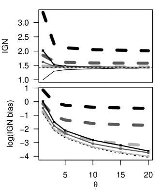
Figure 8: Same as Figure 7 but for skewed distributions. See text for the definition of the non-Normality parameter $\theta$.

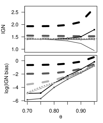
Figure 9: Same as Figure 7 but for bimodal distributions. See text for the definition of the non-Normality parameter $\theta$.

We illustrate the effect of nonnormality on the Ignorance score for Normal ensembles by simulating artificial data from the three types of nonnormal distributions for different values of the non-Normality parameter $\theta$, and for different values of the ensemble size $m$. For each combination of $\theta$ and $m$ we have simulated data sets of $10^{6}$ pairs of ensemble forecasts and observations. For each data set we have then calculated the average of each of the four Ignorance scores described above. The results are illustrated in Figure 7, Figure 8, and Figure 9 for heavy-tailed, skewed, and bimodal distributions, respectively.

In the upper panel of Figure 7 the average Ignorance scores are shown as a function of $\theta$ for the heavy-tailed t-distribution. Due to convergence to Normality, the score of the continuous Normal approximation $\mathcal{I}_{n}$ and the score of the correct t-distribution $\mathcal{I}_{p}$ converge for $\theta\rightarrow\infty$. That is, the bias due to the Normal approximation vanishes for large $\theta$, as expected. The standard Ignorance scores of small ensembles are much larger than both, $\mathcal{I}_{p}$ and $\mathcal{I}_{n}$. The differences decrease as the distribution becomes more Normal (i.e. for higher $\theta$), and as the ensembles get larger. The average values of $\mathcal{I}^{*}$ are always closer to the population Ignorance score $\mathcal{I}_{p}$ of the true t-distribution than the corresponding values of $\widehat{\mathcal{I}}$, i.e. the bias is reduced by $\mathcal{I}^{*}$, albeit not removed completely.

The biases of $\mathcal{I}_{n}$, $\widehat{\mathcal{I}}$ and $\mathcal{I}^{*}$, i.e. their average absolute differences to the score of the true t-distribution, $\mathcal{I}_{p}$, are shown in the lower panel of Figure 7. The bias of $\mathcal{I}^{*}$ is close to the bias of $\mathcal{I}_{n}$. That is, the bias correction of $\mathcal{I}^{*}$ reduces the bias due the finiteness of the ensemble, and provides an approximation of the score that an infinitely large ensemble would achieve under a Normal approximation. The bias of $\mathcal{I}^{*}$ is consistently smaller than the bias of $\widehat{\mathcal{I}}$, even though the assumptions that were made to derive $\mathcal{I}^{*}$ are not satisfied. In summary, $\mathcal{I}^{*}$ cannot remove the bias due to the deviation from Normality, but it does reduce the bias due to the finiteness of the ensemble.

Figure 8, which summarizes the results for the skewed ensemble data, looks qualitatively similar to Figure 7. One striking difference is that, for large ensembles with $m=50$ members, the bias of $\mathcal{I}^{*}$ is considerably larger than the bias of $\mathcal{I}_{n}$ in the case of the t-distribution (Figure 7), but it is almost identical to the bias of $\mathcal{I}_{n}$ for the Gamma distribution. That means that $\mathcal{I}^{*}$ provides a better approximation to $\mathcal{I}_{n}$ in the skewed case than in the heavy-tailed case. The biases in the bimodal case are illustrated in Figure 9. As for the other two types of non-Normality, the biases of $\mathcal{I}^{*}$ are generally smaller than the biases of $\widehat{\mathcal{I}}$. Interestingly, the bias of $\mathcal{I}^{*}$ is even smaller than the bias of $\mathcal{I}_{n}$ in some cases. The general message from Figure 7, Figure 8, and Figure 9 is clear: $\mathcal{I}^{*}$ is systematically less biased than $\widehat{\mathcal{I}}$, even if the ensemble members are not exactly Normal distributed.

References

- Abramowitz and Stegun [1972] M. Abramowitz and I. A. Stegun. Handbook of mathematical functions: with formulas, graphs, and mathematical tables. Courier Dover Publications, 1972. ISBN 0-486-61272-4.
- Anderson [1996] J. L. Anderson. A method for producing and evaluating probabilistic forecasts from ensemble model integrations. Journal of Climate, 9(7):1518–1530, 1996. doi: 10.1175/1520-0442(1996)009¡1518:AMFPAE¿2.0.CO;2.
- Barnston et al. [2010] A. G. Barnston, S. Li, S. J. Mason, D. G. DeWitt, L. Goddard, and X. Gong. Verification of the first 11 years of iri’s seasonal climate forecasts. J. Appl. Meteor. Climatol., 49(3):493–520, Mar 2010. ISSN 1558-8432. doi: 10.1175/2009jamc2325.1.
- Benedetti [2010] R. Benedetti. Scoring rules for forecast verification. Monthly Weather Review, 138(1):203–211, Jan 2010. ISSN 1520-0493. doi: 10.1175/2009mwr2945.1.
- Bröcker and Smith [2008] J. Bröcker and L. A. Smith. From ensemble forecasts to predictive distribution functions. Tellus A, 60(4):663–678, 2008. doi: 10.1111/j.1600-0870.2008.00333.x.
- Buizza and Palmer [1998] R. Buizza and T. N. Palmer. Impact of ensemble size on ensemble prediction. Monthly Weather Review, 126(9):2503–2518, 1998. doi: 10.1175/1520-0493(1998)126¡2503:IOESOE¿2.0.CO;2.
- Dee et al. [2011] D. Dee, S. Uppala, A. Simmons, P. Berrisford, P. Poli, S. Kobayashi, U. Andrae, M. Balmaseda, G. Balsamo, P. Bauer, et al. The ERA-Interim reanalysis: Configuration and performance of the data assimilation system. Quarterly Journal of the Royal Meteorological Society, 137(656):553–597, 2011. doi: 10.1002/qj.828.
- DelSole and Tippett [2007] T. DelSole and M. K. Tippett. Predictability: Recent insights from information theory. Reviews of Geophysics, 45(4), 2007. doi: 10.1029/2006RG000202.
- Déqué et al. [1994] M. Déqué, J. Royer, R. Stroe, and M. France. Formulation of gaussian probability forecasts based on model extended-range integrations. Tellus A, 46(1):52–65, 1994. doi: 10.1034/j.1600-0870.1994.00005.x.
- Du and Smith [2012] H. Du and L. A. Smith. Parameter estimation through ignorance. Phys. Rev. E, 86(1), Jul 2012. ISSN 1550–2376. doi: 10.1103/physreve.86.016213.
- ECOMS User Data Gateway [2014] ECOMS User Data Gateway, 2014. http://meteo.unican.es/ecoms-udg (accessed on 25 June 2014) The ECOMS User Data Gateway is partially funded by the European Union’s Seventh Framework Programme [FP7/2007-2013] under Grant Agreement no 308291 (EUPORIAS).
- Ferro [2007] C. A. T. Ferro. Comparing probabilistic forecasting systems with the Brier score. Weather and Forecasting, 22(5):1076–1088, 2007. doi: 10.1175/WAF1034.1.
- Ferro [2013] C. A. T. Ferro. Fair scores for ensemble forecasts. Quarterly Journal of the Royal Meteorological Society, 2013. doi: 10.1002/qj.2270.
- Ferro et al. [2008] C. A. T. Ferro, D. S. Richardson, and A. P. Weigel. On the effect of ensemble size on the discrete and continuous ranked probability scores. Meteorological Applications, 15(1):19–24, 2008. doi: 10.1002/met.45.
- Fricker et al. [2013] T. E. Fricker, C. A. T. Ferro, and D. B. Stephenson. Three recommendations for evaluating climate predictions. Meteorological Applications, 20(2):246–255, 2013. doi: 10.1002/met.1409.
- Gneiting and Raftery [2005] T. Gneiting and A. E. Raftery. Weather forecasting with ensemble methods. Science, 310(5746):248–249, 2005. doi: 10.1126/science.1115255.
- Gneiting and Raftery [2007] T. Gneiting and A. E. Raftery. Strictly proper scoring rules, prediction, and estimation. Journal of the American Statistical Association, 102(477):359–378, 2007. doi: 10.1198/016214506000001437.
- Gneiting et al. [2005] T. Gneiting, A. E. Raftery, A. H. Westveld III, and T. Goldman. Calibrated probabilistic forecasting using ensemble model output statistics and minimum CRPS estimation. Monthly Weather Review, 133(5), 2005. doi: 10.1175/MWR2904.1.
- Good [1952] I. J. Good. Rational decisions. Journal of the Royal Statistical Society. Series B (Methodological), pages 107–114, 1952. URL http://www.jstor.org/stable/2984087.
- Hagedorn and Smith [2009] R. Hagedorn and L. A. Smith. Communicating the value of probabilistic forecasts with weather roulette. Meteorological Applications, 16(2):143–155, Jun 2009. ISSN 1469-8080. doi: 10.1002/met.92.
- Hogben et al. [1961] D. Hogben, R. Pinkham, and M. Wilk. The moments of the non-central t-distribution. Biometrika, 48(3-4):465–468, 1961. URL http://www.jstor.org/stable/2332772.
- Jolliffe and Stephenson [2012] I. T. Jolliffe and D. B. Stephenson. Forecast Verification: A Practitioner’s Guide in Atmospheric Science. John Wiley & Sons, 2012. ISBN 978-0-470-66071-3.
- Krakauer et al. [2013] N. Y. Krakauer, M. D. Grossberg, I. Gladkova, and H. Aizenman. Information content of seasonal forecasts in a changing climate. Advances in Meteorology, 2013:1–12, 2013. ISSN 1687-9317. doi: 10.1155/2013/480210.
- Lehmann and Casella [1998] E. L. Lehmann and G. Casella. Theory of Point Estimation. Springer, 1998. ISBN 0-387-98502-6.
- MacKay [2003] D. MacKay. Information Theory, Inference, and Learning Algorithms. Cambridge University Press, 2003. ISBN 978-0-521-64298-9.
- Molteni et al. [2011] F. Molteni, T. Stockdale, M. Balmaseda, G. Balsamo, R. Buizza, L. Ferranti, L. Magnusson, K. Mogensen, T. Palmer, and F. Vitart. The new ECMWF seasonal forecast system (System 4), 2011. ECMWF Technical Memorandum No. 656 URL http://old.ecmwf.int/publications/library/ecpublications/_pdf/tm/601-700/tm656.pdf.
- Mood [1950] A. M. Mood. Introduction to the Theory of Statistics. McGraw-hill, 1950. ISBN 0-07-042864-6.
- Müller et al. [2005] W. Müller, C. Appenzeller, F. Doblas-Reyes, and M. Liniger. A debiased ranked probability skill score to evaluate probabilistic ensemble forecasts with small ensemble sizes. Journal of Climate, 18(10):1513–1523, 2005. doi: 10.1175/JCLI3361.1.
- Peirolo [2011] R. Peirolo. Information gain as a score for probabilistic forecasts. Meteorological Applications, 18(1):9–17, Feb 2011. ISSN 1350-4827. doi: 10.1002/met.188.
- Richardson [2001] D. S. Richardson. Measures of skill and value of ensemble prediction systems, their interrelationship and the effect of ensemble size. Quarterly Journal of the Royal Meteorological Society, 127(577):2473–2489, 2001. doi: 10.1002/qj.49712757715.
- Rodrigues et al. [2014] L. R. L. Rodrigues, J. García-Serrano, and F. Doblas-Reyes. Seasonal forecast quality of the west african monsoon rainfall regimes by multiple forecast systems. Journal of Geophysical Research: Atmospheres, 119(13):7908–7930, Jul 2014. ISSN 2169-897X. doi: 10.1002/2013jd021316.
- Roulston and Smith [2002] M. S. Roulston and L. A. Smith. Evaluating probabilistic forecasts using information theory. Monthly Weather Review, 130(6), 2002. doi: 10.1175/1520-0493(2002)130¡1653:EPFUIT¿2.0.CO;2.
- Sivillo et al. [1997] J. K. Sivillo, J. E. Ahlquist, and Z. Toth. An ensemble forecasting primer. Weather and Forecasting, 12(4):809–818, 1997. doi: 10.1175/1520-0434(1997)012¡0809:AEFP¿2.0.CO;2.
- Smith et al. [2014] L. A. Smith, H. Du, E. B. Suckling, and F. Niehörster. Probabilistic skill in ensemble seasonal forecasts. Quarterly Journal of the Royal Meteorological Society, pages n/a–n/a, Jul 2014. ISSN 0035-9009. doi: 10.1002/qj.2403.
- Weedon et al. [2011] G. Weedon, S. Gomes, P. Viterbo, W. Shuttleworth, E. Blyth, H. Österle, J. Adam, N. Bellouin, O. Boucher, and M. Best. Creation of the WATCH Forcing data and its use to assess global and regional reference crop evaporation over land during the twentieth century. J. Hydrometerol., 12:823–848, 2011. doi: 10.1175/2011JHM1369.1.
- Winkler et al. [1996] R. L. Winkler, J. Munoz, J. L. Cervera, J. M. Bernardo, G. Blattenberger, J. B. Kadane, D. V. Lindley, A. H. Murphy, R. M. Oliver, and D. Ríos-Insua. Scoring rules and the evaluation of probabilities. Test, 5(1):1–60, 1996. doi: 10.1080/01621459.1969.10501037.
- Zhu [2005] Y. Zhu. Ensemble forecast: A new approach to uncertainty and predictability. Advances in atmospheric sciences, 22(6):781–788, 2005. doi: 10.1007/BF02918678.