Coherent quantum transport in disordered systems: A unified polaron treatment of hopping and band-like transport

Abstract

Quantum transport in disordered systems is studied using a polaron-based master equation. The polaron approach is capable of bridging the results from the coherent band-like transport regime governed by the Redfield equation to incoherent hopping transport in the classical regime. A non-monotonic dependence of the diffusion coefficient is observed both as a function of temperature and system-phonon coupling strength. In the band-like transport regime, the diffusion coefficient is shown to be linearly proportional to the system-phonon coupling strength, and vanishes at zero coupling due to Anderson localization. In the opposite classical hopping regime, we correctly recover that the dynamics are described by the Fermi’s Golden Rule (FGR) and establish that the scaling of the diffusion coefficient depends on the phonon bath relaxation time. In both the hopping and band-like transport regimes, it is demonstrated that at low temperature the zero-point fluctuations of the bath lead to non-zero transport rates, and hence a finite diffusion constant. Application to rubrene and other organic semiconductor materials shows a good agreement with experimental mobility data.

I Introduction

Quantum transport in disordered systems governs a host of fundamental physical processes including the efficiency of light harvesting systems, organic photovoltaics, conducting polymers, and J-aggregate thin films Podzorov et al. (2004); Troisi and Orlandi (2006); Sakanoue and Sirringhaus (2010); Singh et al. (2009); Dykstra et al. (2008); Bednarz et al. (2003); Moix et al. (2011); Lee et al. (2007); Trambly de Laissardière et al. (2006); Coropceanu et al. (2007); Ortmann et al. (2009); Ciuchi et al. (2011); Tao et al. (2012); Cheng and Silbey (2008). However, our theoretical understanding of these processes is still lacking in many cases. At the most basic level, one may describe the energy transport as a quantum diffusion process occurring in a system that is influenced by both static disorder and thermal fluctuations. Theories based on FGR, i.e. the Marcus or Förster rate expressions, are often used to study the transport properties of disordered organic systems, but only in very few cases, such as the transport in organic crystals, do the dynamics reside in a regime that is amenable to perturbative treatments Bednarz et al. (2004). More commonly, the coupling between the excitonic system and the environment is neither large nor small so that these perturbative treatments often yield qualitatively incorrect results. This is particularly true in the case of biological light harvesting complexes which are among the most efficient energy transporting systems currently known.

Recently, the Haken-Strobl model Moix et al. (2013) and an approximate stochastic Schrödinger equation Zhong et al. (2014) have been used to study the energy transport processes in one-dimensional disordered systems. However, the Haken-Strobl model represents a vast simplification of the true dynamics that is applicable only in the high temperature Markovian limit, while the approximate stochastic Schrödinger equation is only valid in the weak system-phonon coupling regime and fails to correctly reproduce the classical hopping dynamics at high temperature. Here we present a complete characterization of the transport properties over the entire range of phonon bath parameters through the development of an efficient and accurate polaron-transformed Redfield master equation (PTRE). In contrast to many standard perturbative treatments, the PTRE allows one to treat systems that are strongly coupled to the phonon baths. Furthermore, the PTRE is still very accurate even if the system and bath are not strongly coupled provided that the bath relaxation time is sufficiently short Lee et al. (2012); Chang et al. (2013). This approach allows us to explore many interesting features of the dynamics that were previously inaccessible.

In the high temperature, incoherent regime, we recover the known scaling relations of hopping transport that are obtained from FGR. If the bath relaxation time is fast, then the diffusion constant, $D$, decreases with temperature as $T^{-1}$ as was found in the previous Haken-Strobl analysis. However, as the bath relaxation time slows, the FGR reduces to the Marcus rates, and the temperature scaling of the diffusion constant transitions to $D\propto T^{-1/2}$. However, these relations hold only in the high-temperature/strong-coupling limit where the dynamics is incoherent. As the temperature or system-bath coupling decreases, quantum coherence begins to play a role and the FGR results quickly break down, leading to a significant underestimation of the true transport rate. In the sufficiently weak damping regime, the PTRE results reduce to those of band-like transport governed by the standard secular Redfield equation (SRE), wherein the diffusion coefficient can be shown to increase linearly with the system-phonon coupling strength. The SRE rates also demonstrate that transport occurs –even at zero temperature– provided that the system-phonon coupling is finite, due to the dephasing interactions from the phonon bath.

This paper is organized as follows. We describe the PTRE used to compute the diffusion coefficient in an infinite, disordered one-dimensional chain in Sec. II. In the following Sec. III, the numerical results are presented and compared with the results from standard SRE and FGR approaches in the weak and strong coupling regimes, respectively. The limiting results allow for the accurate determination of the respective scaling relations of the diffusion coefficient in each case. The PTRE is used to study some common organic semiconductor materials in Sec. IV. Finally, we conclude with a summary of the results in Sec. V.

II Theory

The total Hamiltonian in the open quantum system formalism is given by

$$H_{\rm tot}=H_{\rm s}+H_{\rm b}+H_{\rm sb},$$ (1)

where the three terms represent Hamiltonians of the system, the phonon bath, and system-bath coupling, respectively. The system is described by a tight binding, Anderson Hamiltonian $H_{\rm s}=\sum_{n}\epsilon_{n}|n\rangle\langle n|+\sum_{m\neq n}J_{mn}|m\rangle\langle n|$, where $|n\rangle$ denotes the site basis and $J_{mn}$ is the electronic coupling between site $m$ and site $n$. Here we only consider one dimensional systems with nearest-neighbor coupling such that $J_{mn}=J(\delta_{m,n+1}+\delta_{m+1,n})$. The static disorder is introduced by taking the site energies, $\epsilon_{n}$, to be independent, identically distributed Gaussian random variables characterized by their variance $\sigma_{n}^{2}=\overline{\epsilon_{n}\epsilon_{n}}$. The overline is used throughout to denote the average over static disorder. We assume that each site is independently coupled to its own phonon bath in the local basis. Thus $H_{\rm b}=\sum_{nk}\omega_{nk}b^{\dagger}_{nk}b_{nk}$ and $H_{\rm sb}=\sum_{nk}g_{nk}|n\rangle\langle n|(b^{\dagger}_{nk}+b_{nk})$, where $\omega_{nk}$ and $b^{\dagger}_{nk}$($b_{nk}$) are the frequency and the creation (annihilation) operator of the $k$-th mode of the bath attached to site $n$ with coupling strength $g_{nk}$, respectively.

Applying the polaron method to study the dynamics of open quantum systems was first proposed by Grover and Silbey Grover and Silbey (1971). This approach has gained a renewed attention due to the recent interest in light harvesting systems McCutcheon and Nazir (2011); Jang et al. (2008) and has recently been extended to study non-equilibrium quantum transport Wang et al. (2014). In this work, we will use a variant of the polaron based master equation which has the same structure as the popular Redfield equation.

In the polaron technique, the unitary transformation operator, $\mbox{e}^{S}=\mbox{e}^{\sum_{nk}\frac{g_{nk}}{\omega_{nk}}|n\rangle\langle n|(b^{\dagger}_{nk}-b_{nk})}$, is applied to the total Hamiltonian

$$\widetilde{H}_{\rm tot}=\mbox{e}^{S}H_{\rm tot}\mbox{e}^{-S}=\widetilde{H}_{\rm s}+\tilde{H}_{\rm b}+\widetilde{H}_{\rm sb},$$ (2)

where $\widetilde{H}_{\rm s}=\sum_{n}\epsilon_{n}|n\rangle\langle n|+\sum_{m\neq n}\kappa_{mn}J_{mn}|m\rangle\langle n|$, $\widetilde{H}_{\rm sb}=\sum_{n\neq m}J_{mn}|m\rangle\langle n|V_{mn}$ and $\widetilde{H}_{\rm b}=H_{\rm b}=\sum_{nk}\omega_{nk}b^{\dagger}_{nk}b_{nk}$. The electronic coupling is renormalized by a constant, $\kappa_{mn}=\mbox{e}^{-\frac{1}{2}\sum_{k}\left[\frac{g_{mk}^{2}}{\omega_{mk}^{2}}\coth(\beta\omega_{mk}/2)+\frac{g_{nk}^{2}}{\omega_{nk}^{2}}\coth(\beta\omega_{nk}/2)\right]}$, with the inverse thermal energy $\beta=1/k_{B}T$. The bath coupling operator now becomes $V_{mn}=\mbox{e}^{\sum_{k}\frac{g_{mk}}{\omega_{mk}}(b^{\dagger}_{mk}-b_{mk})}\mbox{e}^{-\sum_{k}\frac{g_{nk}}{\omega_{nk}}(b^{\dagger}_{nk}-b_{nk})}-\kappa_{mn}$, and is constructed such that its thermal average is zero, i.e. $\mbox{tr}_{\rm b}[V_{mn}\mbox{e}^{-\beta H_{\rm b}}]=0$. Additionally, we assume the coupling constants are identical across all sites $g_{nk}=g_{k}$ and a super-Ohmic spectral density, $J(\omega)=\pi\sum_{k}g_{k}^{2}\delta(\omega-\omega_{k})=\gamma\omega^{3}\mbox{e}^{-\omega/\omega_{c}}$ where $\gamma$ is the dissipation strength and $\omega_{c}$ is the cut-off frequency.

A detailed derivation of PTRE is given in Appendix A, here we only summarize the main results. A perturbation approximation is applied in terms of the transformed system-bath coupling leading to a PTRE for the transformed reduced density matrix, $\widetilde{\rho}_{s}$:

$$\frac{d\widetilde{\rho}_{\nu\nu}(t)}{dt} = \sum_{\nu^{\prime}}R_{\nu\nu,\nu^{\prime}\nu^{\prime}}\widetilde{\rho}_{\nu^{\prime}\nu^{\prime}}(t);$$ (3)

$$\frac{d\widetilde{\rho}_{\mu\nu}(t)}{dt} = (-\mathrm{i}\,\omega_{\nu\mu}+R_{\mu\nu,\mu\nu})\widetilde{\rho}_{\mu\nu}(t),\,\,\,\,\,\mbox{$\nu\neq\mu$},$$ (4)

where the Markov and secular approximations have also been employed. The Greek indices denote the eigenstates of the polaron transformed system Hamiltonian, i.e. $\widetilde{H}_{\rm s}|\mu\rangle=\widetilde{E}_{\mu}|\mu\rangle$ and $\omega_{\mu\nu}=\widetilde{E}_{\mu}-\widetilde{E}_{\nu}$. The Redfield tensor, $R_{\mu\nu,\mu^{\prime}\nu^{\prime}}$, describes the phonon-induced relaxation and can be expressed as

$$R_{\mu\nu,\mu^{\prime}\nu^{\prime}} =\Gamma_{\nu^{\prime}\nu,\mu\mu^{\prime}}+\Gamma_{\mu^{\prime}\mu,\nu\nu^{\prime}}^{*}-\delta_{\nu\nu^{\prime}}\sum_{\kappa}\Gamma_{\mu\kappa,\kappa\mu^{\prime}}-\delta_{\mu\mu^{\prime}}\sum_{\kappa}\Gamma_{\nu\kappa,\kappa\nu^{\prime}}^{*};$$ (5)

$$\Gamma_{\mu\nu,\mu^{\prime}\nu^{\prime}} =\sum_{mnm^{\prime}n^{\prime}}J_{mn}J_{m^{\prime}n^{\prime}}\langle\mu|m\rangle\langle n|\nu\rangle\langle\mu^{\prime}|m^{\prime}\rangle\langle n^{\prime}|\nu^{\prime}\rangle K_{mn,m^{\prime}n^{\prime}}(\omega_{\nu^{\prime}\mu^{\prime}})\;,$$ (6)

where $K_{mn,m^{\prime}n^{\prime}}(\omega)$ is the half-Fourier transform of the bath correlation function

$$K_{mn,m^{\prime}n^{\prime}}(\omega)=\int^{\infty}_{0}\mbox{e}^{\mathrm{i}\omega t}\langle V_{mn}(t)V_{m^{\prime}n^{\prime}}(0)\rangle_{H_{\rm b}}dt\;,$$ (7)

and $\langle V_{mn}(t)V_{m^{\prime}n^{\prime}}(0)\rangle_{H_{\rm b}}=\mbox{tr}_{\rm b}[\mbox{e}^{-\beta H_{\rm b}}V_{mn}(t)V_{m^{\prime}n^{\prime}}(0)]/\mbox{tr}_{\rm b}[\mbox{e}^{-\beta H_{\rm b}}]$. Since the system is disordered and we are mainly interested in the long time dynamics, the Markov and secular approximations do not incur a significant loss of accuracy. Comparison of the dynamics computed with and without these approximations shows little discrepancy (see Appendix A). It should be noted that the transformed reduced density matrix, $\widetilde{\rho}_{s}$, is different from the reduced density matrix in the original frame, $\rho_{s}$. However, for the transport properties studied here, only the population dynamics is needed which is invariant under the polaron transformation since $\widetilde{\rho}_{nn}(t)=\rho_{nn}(t)$.

Diffusion - In the presence of both disorder and dissipation, we find empirically that after an initial transient time that is approximately proportional to $J^{3}\beta/\gamma$, the mean square displacement, $\overline{\langle R^{2}(t)\rangle}=\overline{\sum_{n}n^{2}\rho_{nn}(t)}$, grows linearly with time, where the origin is defined such that $\langle R^{2}(0)\rangle=0$. The diffusion constant, $D$, can then be defined as $\lim_{t\rightarrow\infty}\overline{\langle R^{2}(t)\rangle}=2Dt$. The electronic coupling $J=1$ sets the energy scale and quantities throughout are implicitly stated in units of $J$. In the numerical simulations, we use a one-dimensional chain of 250-300 sites and average over 100-500 realizations of static disorder sampled from a Gaussian distribution with variance $\sigma=1$. The number of realizations needed for convergence is highly dependent on the temperature; more samples are needed in the low temperature regime.

III Results

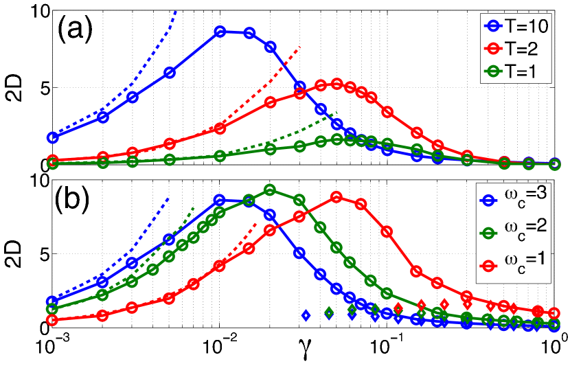
Figure 1: The diffusion constant as a function of the dissipation strength, $\gamma$. The dashed lines display the corresponding results from the SRE, while diamond symbols depict the results of the FGR rates given in Equation 8. (a) Results for different temperatures and a fast bath $\omega_{c}=3$. (b) Results for different cut-off frequencies and $T=10$.

We first investigate the effect of the dissipation strength, $\gamma$, on the diffusion constant in Figure 1. A non-monotonic dependence of $D$ as a function of $\gamma$ is observed, consistent with the previous studies using the Haken-Strobl model Moix et al. (2013). Without coupling to the bath, there is no macroscopic transport since all the wavefunctions in the one-dimensional disordered system are Anderson localized. Introducing dissipation destroys the phase coherence that gives rise to localization, allowing for transport to occur. Therefore in the weak coupling regime, increasing $\gamma$ leads to faster transport as is readily apparent from the SRE rates in Equation 6, and thus $D$ increases linearly with $\gamma$. In the opposite regime of strong coupling, the coherence generated between sites is quickly destroyed and the quantum transport reduces to a classical hopping dynamics between neighboring sites. In this regime, the dissipation strength effectively acts as classical friction that impedes the transport Cao and Silbey (2009) leading $D$ to behave as a decreasing function of $\gamma$ as is observed in Figure 1. The interplay between static disorder and dissipation thus gives rise to an optimal dissipation strength for transport. In Figure 1 (a), it is seen that the maximal diffusive rate both increases and shifts to smaller coupling strengths as the temperature increases since thermal fluctuations also assist the quantum system to overcome the localization barriers in the weak coupling regime. For comparison, we also include the results from the SRE in the weak coupling regime. For small $\gamma$ and $T$, the SRE provides a reliable description of the transport properties, but starts to breakdown as $\gamma$ (or $T$) increases leading to an unphysical $D\propto\gamma$ dependence. The breakdown of the SRE has been discussed by Ishizaki and Fleming for a two-site model Ishizaki and Fleming (2009) and by Wu et al. for FMO Wu et al. (2010).

Figure 1 (b) depicts $D$ as a function of $\gamma$ for different bath cut-off frequencies. It is found that the large $\gamma$ scaling of $D$ is highly dependent on the relaxation time of the bath. For a fast bath, the rates decrease approximately as $1/\gamma$ consistent with our previous analysis of the Haken-Strobl model Moix et al. (2013). However, as the bath frequency decreases, a transition from the $1/\gamma$ dependence to $1/\sqrt{\gamma}$ dependence is observed. This can be rationalized by noting that in the high temperature and strong damping regime, the dynamics are incoherent and can be described by classical hopping between nearest neighbors. Then the hopping rate between sites $m$ and $n$ is accurately determined from FGR:

$$k_{F}(\Delta_{mn})=J_{mn}^{2}\kappa_{mn}^{2}\,\mbox{Re}\int^{\infty}_{-\infty}dt\,\,\mbox{e}^{\mathrm{i}\Delta_{mn}t}[\mbox{e}^{g(t)}-1],$$ (8)

and

$$g(t)=2\int^{\infty}_{0}\frac{d\omega}{\pi}\frac{J(\omega)}{\omega^{2}}\Big{[}\coth\frac{\beta\omega}{2}\cos\omega t-\mathrm{i}\sin\omega t\Big{]},$$ (9)

where $\Delta_{mn}=\epsilon_{m}-\epsilon_{n}$ is the activation barrier, and $J_{mn}$ is the electronic coupling. In the slow bath limit the above expression reduces to the Marcus rate $k_{M}(\Delta)\approx\frac{\pi}{2}J^{2}\sqrt{\frac{\beta}{\gamma\omega_{c}^{3}}}\mbox{e}^{-\frac{\beta(\pi\Delta-4\gamma\omega_{c}^{3})^{2}}{16\pi\gamma\omega_{c}^{3}}}$ which captures the correct $1/\sqrt{\gamma T}$ dependence of the rate. Defining the energy transfer time as the inverse of the rate, $\tau_{F}(\Delta)=1/k_{F}(\Delta)$, static disorder can be introduced by averaging $\tau_{F}(\Delta)$ over the Gaussian distribution of static disorder: $\overline{\tau_{F}}=\int P(\Delta)\tau_{F}(\Delta)d\Delta$ where $P(\Delta)=\frac{1}{\sigma^{\prime}\sqrt{2\pi}}\mbox{e}^{-\Delta^{2}/2\sigma^{\prime 2}}$ and $\sigma^{\prime 2}=\overline{\Delta_{mn}^{2}}=2\sigma^{2}$. The disorder-averaged golden rule rate can then be obtained using $\overline{k_{F}}=1/\overline{\tau_{F}}$ and is plotted in Figure 1 (b). While it is seen to capture the correct scaling of $D$ in the overdamped regime, it significantly underestimates the transport in the small and intermediate damping regimes. As the dynamics becomes more coherent, the classical hopping rate between sites provides a qualitatively incorrect description of the transport. In the sufficiently weak dephasing regime, the dynamics from the PTRE reduce to those of the standard SRE (dashed lines in Figure 1 (b)).

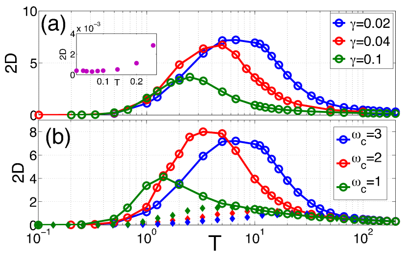
Figure 2: The diffusion constant as a function of temperature. (a) Results for different values of dissipation strength and a fast bath $\omega_{c}=3$. The inset shows the diffusion constant calculated with the SRE near zero temperature and $\gamma=0.01$. (b) Results for different cut-off frequencies and a constant reorganization energy of $\int^{\infty}_{0}\frac{J(\omega)}{\omega}=1.08$. The diamond symbols depict the results of the FGR rates as given by Equation 8.

While the $\gamma$ dependence of $D$ provides many physical insights, the temperature dependence is more experimentally accessible, and is presented in Figure 2. Similar to the $\gamma$ dependence, $D$ exhibits a non-monotonic dependence of $T$ and the high $T$ scaling is sensitive to the cut-off frequency of the bath, as shown in Figure 2 (b). At high temperature, we observe $D$ decreases as $1/\sqrt{T}$ for a slow bath as predicted by the Marcus theory, while for a fast bath, we recover the Haken-Strobl scaling of $1/T$. The system-bath coupling strengths shown in Figure 2 (a) lie to the right of the maxima in Figure 1. Hence $D$ decreases as $\gamma$ increases in the high temperature regime. In the opposite low temperature regime, the intermediate coupling results shown in Figure 2 (a) are beyond the reach of the SRE. Thus $D$ does not increase at a rate proportional to $\gamma$ as might be expected. However, the results here also do not agree with the Marcus formula where one would expect the transport rate to decrease as $1/\sqrt{\gamma T}$, but instead the diffusion constants are nearly independent of $\gamma$. This low temperature, intermediate coupling regime is not adequately described by either of the perturbative methods. At zero temperature, quantum fluctuations from the thermal environment are still present to destroy the Anderson localization and allow for transport to occur, albeit at a very slow rate. This leads to a small but finite value of $D$ as seen in the inset of Figure 2 (a).

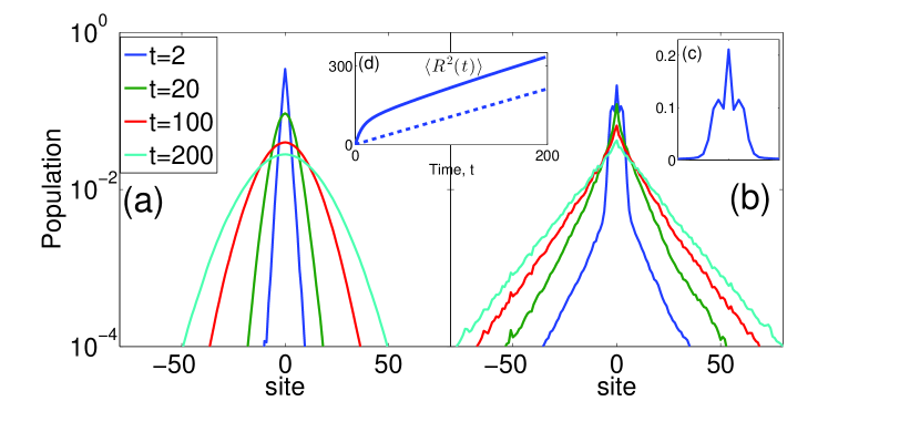
Figure 3: Time evolution of the probability distribution profiles for $\gamma=0.02$, $\omega_{c}=3$ and (a) high temperature, $T=50$ or (b) low temperature $T=1$. The diffusion constant is $2D\approx 1.1$ in both cases. The inset (c) shows the low temperature wavelike population profile at $t=2$ in linear scale. The inset (d) shows the respective mean-squared displacements $\langle R^{2}(t)\rangle$ for $T=1$ (solid) and $T=50$ (dashed).

In addition to the steady state transport properties, it is also useful to explore the dynamics of noisy, disordered systems. Figure 3 displays the average population probability distribution at high and low temperatures for an initial excitation located at the center of the disordered chain. The temperatures are selected such that the diffusion constants in Figure 3 (a) and (b) are approximately the same, $2D\approx 1.1$. In the high temperature case, the coherence is quickly destroyed by dissipation, no wavelike motion is observed in the time scale plotted. While the population distribution appears exponential at short times –which is a signature of Anderson localization– the exponential behavior quickly transitions to a Gaussian profile indicating the onset of the diffusive regime. The population dynamics at low temperature in Figure 3 (b) is qualitatively different. At short times, the distribution near the center of the chain (Figure 3 (c)) displays wavelike motion characteristic of free-particle dynamics while the tails decay exponentially. The wavelike motion disappears at intermediate times but the localization peak near the center persists. Although the exponential tail eventually disappears, the transition of the population distribution to a Gaussian form is slow and takes place long after a reliable estimate of $D$ can been obtained $\left(\overline{\langle R^{2}\rangle}\propto t\right)$, as shown in inset of the Figure 3 (d).

IV Applications

It is interesting to compare estimates of the transport properties in real material systems from the PTRE with the approximate FGR and SRE rates that are often assumed to hold. For example, predictions of the charge mobility, $\mu=\frac{eD}{k_{\rm B}T}$, of several commonly used organic semiconductors are presented in Table 1. The parameters are taken from Ref. Stehr et al. (2011) and we use the directions with the largest electronic couplings. Despite using a vastly simplified model, the mobility calculated with the PTRE is in reasonable agreement with the available experimental values, while the SRE usually leads to an substantial overestimation of the mobility and the commonly used FGR generally leads to a significant underestimation because of the neglect of quantum coherence.

V Conclusion

We have developed a polaron-transformed Redfield equation to systematically study the transport properties of disordered systems in the presence of quantum phonon modes, and established scaling relations for the diffusion coefficients at both limits of the temperature and system-bath coupling strength. The results presented here constitute one of the first studies of quantum transport in extended disordered systems over the complete range of phonon bath parameters. The PTRE provides a general framework to establish a unified understanding of the transport properties of a wide variety of systems including light-harvesting complexes, organic photovoltaics, conducting polymers and J-aggregate thin films.

VI acknowledgement

This work was supported by the NSF (Grant No. CHE-1112825) and DARPA (Grant No. N99001-10-1-4063). C. K. Lee acknowledges support by the Ministry of Education (MOE) and National Research Foundation of Singapore. J. Moix has been supported by the Center for Excitonics, an Energy Frontier Research Center funded by the US Department of Energy, Office of Science, Office of Basic Energy Sciences under Award No. DE-SC0001088.

Appendix A Derivation of the Polaron-Transformed Master Equation

The total Hamiltonian of the system and the bath is

$$H_{tot} = H_{s}+H_{b}+H_{sb},$$

$$= \sum_{n}\epsilon_{n}|n\rangle\langle n|+\sum_{m\neq n}J_{mn}|m\rangle\langle n|+\sum_{n}\sum_{k}\omega_{nk}b^{\dagger}_{nk}b_{nk}+\sum_{n}\sum_{k}g_{nk}|n\rangle\langle n|(b^{\dagger}_{nk}+b_{nk}),$$

where $|n\rangle$ denotes the site basis, $\epsilon_{n}$ is the site energy, and $J_{nm}$ is the electronic coupling between site $n$ and site $m$. Each site is independently coupled to its own phonon bath in the local basis. The variable $\omega_{nk}$ and operator $b^{\dagger}_{nk}$($b_{nk}$) are the frequency and the creation (annihilation) operator of the $k$-th mode of the bath attached to site $n$ with coupling strength $g_{nk}$, respectively.

Applying the polaron transformation, $\mbox{e}^{S}=\mbox{e}^{\sum_{nk}\frac{g_{nk}}{\omega_{nk}}|n\rangle\langle n|(b^{\dagger}_{nk}-b_{nk})}$, to the total Hamiltonian, we obtain

$$\widetilde{H}_{tot} = \mbox{e}^{S}H_{tot}\mbox{e}^{-S}=\widetilde{H}_{s}+\widetilde{H}_{b}+\widetilde{H}_{sb};$$ (11)

$$\widetilde{H}_{s} = \sum_{n}\epsilon_{n}|n\rangle\langle n|+\sum_{m\neq n}\kappa_{mn}J_{mn}|m\rangle\langle n|;$$ (12)

$$\widetilde{H}_{b} = H_{b}=\sum_{n}\sum_{k}\omega_{nk}b^{\dagger}_{nk}b_{nk};$$ (13)

$$\widetilde{H}_{sb} = \sum_{m\neq n}J_{mn}|m\rangle\langle n|V_{mn},$$ (14)

where the electronic coupling is renormalized by the constant, $\kappa_{mn}=\mbox{e}^{-\frac{1}{2}\sum_{k}\frac{g_{mk}^{2}}{\omega_{mk}^{2}}\coth(\beta\omega_{mk}/2)-\frac{1}{2}\sum_{k}\frac{g_{nk}^{2}}{\omega_{nk}^{2}}\coth(\beta\omega_{nk}/2)}$ and $\beta=1/k_{B}T$. Tildes are used to denote operators in the polaron frame. The bath coupling operator now becomes $V_{mn}=\mbox{e}^{\sum_{k}\frac{g_{mk}}{\omega_{mk}}(b^{\dagger}_{mk}-b_{mk})}\mbox{e}^{-\sum_{k}\frac{g_{nk}}{\omega_{nk}}(b^{\dagger}_{nk}-b_{nk})}-\kappa_{mn}$. The bath coupling term is constructed such that its thermal average is zero, $\mbox{tr}_{b}[V_{mn}\mbox{e}^{-\beta H_{b}}]=0$. Assuming the coupling constants are identical across all sites $g_{nk}=g_{k}$ and introducing the spectral density $J(\omega)=\pi\sum_{k}g_{k}^{2}\delta(\omega-\omega_{k})$, the renormalization constant can then be written as $\kappa=\kappa_{mn}=\mbox{e}^{-\int^{\infty}_{0}\frac{d\omega}{\pi}\frac{J(\omega)}{\omega^{2}}\coth(\beta\omega/2)}$. Here we use a super Ohmic spectral density $J(\omega)=\gamma\omega^{3}\mbox{e}^{-\omega/\omega_{c}}$ where $\gamma$ is the dissipation strength and $\omega_{c}$ is the cut-off frequency.

To derive the master equation, let us first introduce the Hubbard operator $X_{\nu\mu}=|\nu\rangle\langle\mu|$, where $|\nu\rangle$ is the eigenstate of the transformed system Hamiltonian: $\widetilde{H_{s}}|\nu\rangle=E_{\nu}|\nu\rangle$. The system reduced density matrix element can be conveniently obtained using the relation $\rho_{\mu\nu}(t)=\mbox{tr}_{s+b}[\rho_{s+b}(0)X_{\nu\mu}(t)]$, as will be done later. The Heisenberg equation of the Hubbard operator is given by

$$\frac{dX_{\nu\mu}(t)}{dt} = \mathrm{i}[\widetilde{H}_{0}(t),X_{\nu\mu}(t)]+\mathrm{i}[\widetilde{H}_{sb}(t),X_{\nu\mu}(t)],$$ (15)

where $\widetilde{H}_{0}=\widetilde{H}_{s}+\widetilde{H}_{b}$ is the free Hamiltonian. We can write the second term as

$$[\widetilde{H}_{sb}(t),X_{\nu\mu}(t)]=U^{\dagger}(t)\,\,[\widetilde{H}_{sb},X_{\nu\mu}]\,\,U(t),$$ (16)

where the evolution operator is $U(t)=\mbox{e}^{-\mathrm{i}\widetilde{H}_{tot}t}$. We then use Kubo’s identity Kubo et al. (1995) to expand $U(t)$ perturbatively in terms of $\widetilde{H}_{sb}$:

$$U(t)\approx\mbox{e}^{-\mathrm{i}\widetilde{H}_{0}t}\left[1-\mathrm{i}\int^{t}_{0}ds\>\widehat{\widetilde{H}}_{sb}(s)\right],$$ (17)

where hats over the operators are used to denote operators in the interaction picture, $\widehat{O}(t)=\mbox{e}^{\mathrm{i}{\widetilde{H}}_{0}t}O\mbox{e}^{-\mathrm{i}\widetilde{H}_{0}t}$. Inserting the expansion into Equation 16 and keeping terms up to second order in $\widetilde{H}_{sb}$, the Heisenberg equation, Equation 15, becomes

$$\frac{dX_{\nu\mu}(t)}{dt}=\mathrm{i}[\widetilde{H}_{0}(t),X_{\nu\mu}(t)]+\mathrm{i}[\widehat{\widetilde{H}}_{sb}(t),\widehat{X}_{\nu\mu}(t)]-\int^{t}_{0}ds\,[\widehat{\widetilde{H}}_{sb}(s),\,[\widehat{\widetilde{H}}_{sb}(t),\widehat{X}_{\nu\mu}(t)]]$$ (18)

We multiply the initial condition, $\widetilde{\rho}_{s+b}(0)$, to the RHS of Equation 18 and perform a total trace of both the system and bath, obtain an equation governing the dynamics of the system reduced density matrix elements

$$\frac{d\widetilde{\rho}_{\mu\nu}(t)}{dt} = -\mathrm{i}\,\omega_{\mu\nu}\widetilde{\rho}_{\mu\nu}(t)-\int^{t}_{0}ds\,\,\mbox{tr}_{s+b}\Big{(}[\widehat{\widetilde{H}}_{SB}(s),\,[\widehat{\widetilde{H}}_{sb}(t),\widetilde{X}_{\nu\mu}(t)]\,]\widetilde{\rho}_{s+b}(0)\Big{)},$$ (19)

where $\omega_{\mu\nu}=E_{\mu}-E_{\nu}$. Assuming factorized initial conditions, $\widetilde{\rho}_{s+b}(0)=\widetilde{\rho}_{s}(0)\otimes\frac{\mbox{e}^{-\beta H_{b}}}{\mbox{tr}[\mbox{e}^{-\beta H_{b}}]}$, and substituting the expression of $\widetilde{H}_{sb}$ into Equation 19, we finally have the master equation after some manipulations

$$\frac{d\tilde{\rho}_{\mu\nu}(t)}{dt}=-\mathrm{i}\omega_{\mu\nu}\tilde{\rho}_{\mu\nu}(t)+\sum_{\mu^{\prime}\nu^{\prime}}R_{\mu\nu,\mu^{\prime}\nu^{\prime}}(t)\tilde{\rho}_{\mu^{\prime}\nu^{\prime}}(t),$$ (20)

where the Redfield tensor, $R_{\mu\nu,\mu^{\prime}\nu^{\prime}}(t)$, describes the phonon-induced relaxation. It can be expressed as

$$R_{\mu\nu,\mu^{\prime}\nu^{\prime}}(t)=\Gamma_{\nu^{\prime}\nu,\mu\mu^{\prime}}(t)+\Gamma_{\mu^{\prime}\mu,\nu\nu^{\prime}}^{*}(t)-\delta_{\nu\nu^{\prime}}\sum_{\kappa}\Gamma_{\mu\kappa,\kappa\mu^{\prime}}(t)-\delta_{\mu\mu^{\prime}}\sum_{\kappa}\Gamma_{\nu\kappa,\kappa\nu^{\prime}}^{*}(t).$$ (21)

The damping rates have the form

$$\Gamma_{\mu\nu,\mu^{\prime}\nu^{\prime}}(t)=\sum_{mnm^{\prime}n^{\prime}}J_{mn}J_{m^{\prime}n^{\prime}}\langle\mu|m\rangle\langle n|\nu\rangle\langle\mu^{\prime}|m^{\prime}\rangle\langle n^{\prime}|\nu^{\prime}\rangle K_{mn,m^{\prime}n^{\prime}}(\omega_{\nu^{\prime}\mu^{\prime}},t),$$ (22)

where $K_{mn,m^{\prime}n^{\prime}}(\omega,t)$ is the integrated bath correlation function

$$K_{mn,m^{\prime}n^{\prime}}(\omega,t)=\int^{t}_{0}\mbox{e}^{\mathrm{i}\omega t}\langle\widehat{V}_{mn}(t)\widehat{V}_{m^{\prime}n^{\prime}}(0)\rangle_{H_{b}}d\omega.$$ (23)

$\langle\bullet\rangle_{H}$ denotes the average over the thermal state $\mbox{e}^{-\beta H}/\mbox{tr}[\mbox{e}^{-\beta H}]$. Assuming a short bath correlation time, we can make the Markov approximation by taking the upper integration limit to infinity, making the damping rate a half-Fourier transform of the bath correlation function. The bath correlation function is given by Jang (2011)

$$\langle V_{mn}(t)V_{m^{\prime}n^{\prime}}(0)\rangle_{H_{b}}=\kappa^{2}(\mbox{e}^{-\lambda_{mn,m^{\prime}n^{\prime}}\phi(t)}-1),$$ (24)

where $\lambda_{mn,m^{\prime}n^{\prime}}=\delta_{mm^{\prime}}-\delta_{mn^{\prime}}+\delta_{nn^{\prime}}-\delta_{nm^{\prime}}$ and

$$\phi(t)=\int^{\infty}_{0}\frac{d\omega}{\pi}\frac{J(\omega)}{\omega^{2}}\Big{[}\cos(\omega t)\coth(\beta\omega/2)\,-\,\mathrm{i}\sin(\omega t)\Big{]}.$$ (25)

A few remarks are in place. First, the decoupled initial condition assumption is generally not true in the polaron frame since $\widetilde{\rho}_{s+b}(0)$ is usually a complicated system-bath entangled state generated by the polaron transformation. This occurs even if the initial state in the original frame does factorize as $\rho_{s+b}=\rho_{s}(0)\otimes\rho_{b}(0)$. Regardless, in most cases, the decoupled initial condition is only an approximation. However, Nazir et al. Kolli et al. (2011) has shown that the error incurred due to the initial condition is only significant at short times. In this work, we are mainly interested in the long time dynamics of the system. Therefore, the accuracy of our results is not considerably affected by the decoupled initial condition approximation. Second, Equation 21 has the same structure as the Redfield equation commonly used in the magnetic resonance literature. The only difference is that the damping tensor $\Gamma_{\mu\nu,\mu^{\prime}\nu^{\prime}}$ contains four summations as opposed to two summations in the standard Redfield equation. In fact, the Redfield equation can be recovered by following the same prescription as described above except without applying the polaron transformation.

Within the secular approximation, the evolution of the diagonal and off-diagonal density matrix elements are decoupled:

$$\frac{d\tilde{\rho}_{\nu\nu}(t)}{dt} = \sum_{\nu^{\prime}}R_{\nu\nu,\nu^{\prime}\nu^{\prime}}\rho_{\nu^{\prime}\nu^{\prime}}(t);$$ (26)

$$\frac{d\tilde{\rho}_{\mu\nu}(t)}{dt} = (-\mathrm{i}\,\omega_{\nu\mu}+R_{\mu\nu,\mu\nu})\tilde{\rho}_{\mu\nu}(t),\,\,\,\,\,\text{$\nu\neq\mu$}.$$ (27)

We compare the results from the above secular polaron master equation with that of the more accurate time-convolutionless second-order polaron master equation Zimanyi and Silbey (2012) without the secular and Markov approximations for an unbiased two-site system. The results are plotted in Figure 4. It can the be seen that the results agree remarkably well for different values of temperature and coupling strength. This demonstrates that the secular and Markov approximations made here do not incur a significant loss of accuracy in our results.

Appendix B Strong Damping Limit

Here we explore the strong system-bath coupling limit of the PTRE. In the strong coupling limit, the coherence is quickly destroyed by dissipation, thus we only need to consider the equations of motion of the population, i.e. Equation 26. Additionally, $\kappa_{mn}\rightarrow 0$ for large $\gamma$, i.e. the eigenbasis of $\widetilde{H}_{s}$ is also the site basis, $|n\rangle$. As a result, Equation 26 becomes the kinetic equations governing the population dynamics. For a two site model, it can be written as:

$$\frac{d\tilde{\rho}_{11}(t)}{dt} = R_{11,11}(t)\rho_{11}(t)+R_{11,22}(t)\rho_{22}(t),$$

$$\frac{d\tilde{\rho}_{22}(t)}{dt} = R_{22,11}(t)\rho_{11}(t)+R_{22,22}(t)\rho_{22}(t).$$ (28)

The transition rate from site $1$ to site $2$ is given by $k_{12}=R_{11,22}=2\mbox{Re}[\Gamma_{21,12}]$. Explicitly,

$$k_{12}=2\kappa^{2}J^{2}\mbox{Re}\int^{t}_{0}dt\,\mbox{e}^{\mathrm{i}\omega_{21}t}(\mbox{e}^{2\phi(t)}-1)$$ (29)

where $\omega_{21}=\omega_{2}-\omega_{1}$. The above transition rate is the same as the prediction from FGR.

	PTRE	Redfield	FGR	Experiment
Rubrene	11.1	41.2	0.33	3 to 15
Pentacene	0.73	2.0	0.045	0.66 to 2.3
PBI-F2	$2.2\times 10^{-5}$	$1.2\times 10^{-3}$	$2.0\times 10^{-5}$	-
PBI-(C4F9)2	0.61	104	0.25	-

Table 1: Mobility (in cm²/Vs) of organic semiconductor materials at $\omega_{c}=500$ cm^-1, $T=300$ K and $\sigma=800$ cm^-1.

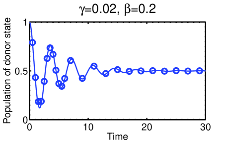
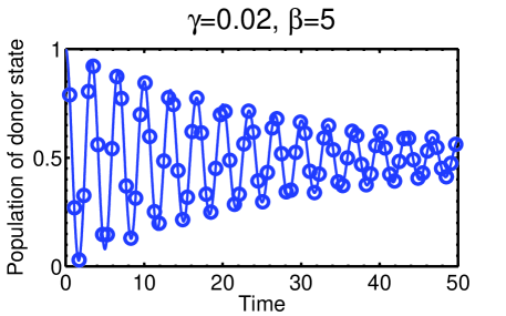
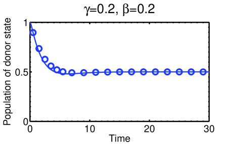
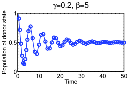
Figure 4: Time evolution of the population dynamics of the donor (site 1) calculated using the secular polaron master equation as given in Equation 26 and Equation 27 (symbols) and the time-convolutionless second-order polaron master equation used in Ref. Zimanyi and Silbey (2012) (solid lines). The parameters used are $\epsilon_{1}=\epsilon_{2}=0$, $J_{12}=1$ and $\omega_{c}=3$.

References

- Podzorov et al. (2004) V. Podzorov, E. Menard, A. Borissov, V. Kiryukhin, J. A. Rogers, and M. E. Gershenson, Phys. Rev. Lett. 93, 086602 (2004).
- Troisi and Orlandi (2006) A. Troisi and G. Orlandi, Phys. Rev. Lett. 96, 086601 (2006).
- Sakanoue and Sirringhaus (2010) T. Sakanoue and H. Sirringhaus, Nature Materials 9, 736 (2010).
- Singh et al. (2009) J. Singh, E. R. Bittner, D. Beljonne, and G. D. Scholes, J. Chem. Phys. 131, 194905 (2009).
- Dykstra et al. (2008) T. E. Dykstra, E. Hennebicq, D. Beljonne, J. Gierschner, G. Claudio, E. R. Bittner, J. Knoester, and G. D. Scholes, J. Phys. Chem. B 113, 656 (2008).
- Bednarz et al. (2003) M. Bednarz, V. A. Malyshev, and J. Knoester, Phys. Rev. Lett. 91, 217401 (2003).
- Moix et al. (2011) J. Moix, J. Wu, P. Huo, D. Coker, and J. Cao, J. Phys. Chem. Lett. 2, 3045 (2011).
- Lee et al. (2007) H. Lee, Y.-C. Cheng, and G. R. Fleming, Science 316, 1462 (2007).
- Trambly de Laissardière et al. (2006) G. Trambly de Laissardière, J.-P. Julien, and D. Mayou, Phys. Rev. Lett. 97, 026601 (2006).
- Coropceanu et al. (2007) V. Coropceanu, J. Cornil, D. A. da Silva Filho, Y. Olivier, R. Silbey, and J.-L. Bredas, Chem. Rev. 107, 926 (2007), ISSN 0009-2665.
- Ortmann et al. (2009) F. Ortmann, F. Bechstedt, and K. Hannewald, Phys. Rev. B 79, 235206 (2009).
- Ciuchi et al. (2011) S. Ciuchi, S. Fratini, and D. Mayou, Phys. Rev. B 83, 081202 (2011).
- Tao et al. (2012) S. Tao, N. Ohtani, R. Uchida, T. Miyamoto, Y. Matsui, H. Yada, H. Uemura, H. Matsuzaki, T. Uemura, J. Takeya, et al., Phys. Rev. Lett. 109, 097403 (2012).
- Cheng and Silbey (2008) Y. Cheng and R. J. Silbey, J. Chem. Phys. 128, 114713 (2008).
- Bednarz et al. (2004) M. Bednarz, V. A. Malyshev, and J. Knoester, J. Chem. Phys. 120, 3827 (2004).
- Moix et al. (2013) J. M. Moix, M. Khasin, and J. Cao, New J. Phys. 15, 085010 (2013).
- Zhong et al. (2014) X. Zhong, Y. Zhao, and J. Cao, New J. Phys. 16, 045009 (2014).
- Lee et al. (2012) C. K. Lee, J. Moix, and J. Cao, J. Chem. Phys. 136, 204120 (2012).
- Chang et al. (2013) H.-T. Chang, P.-P. Zhang, and Y.-C. Cheng, J. Chem. Phys. 139, 224112 (2013).
- Grover and Silbey (1971) M. Grover and R. Silbey, J. Chem. Phys. 54, 4843 (1971).
- McCutcheon and Nazir (2011) D. P. S. McCutcheon and A. Nazir, Phys. Rev. B 83, 165101 (2011).
- Jang et al. (2008) S. Jang, Y.-C. Cheng, D. R. Reichman, and J. D. Eaves, J. Chem. Phys. 129, 101104 (2008).
- Wang et al. (2014) C. Wang, J. Ren, and J. Cao, arXiv:1410.4366 (2014).
- Cao and Silbey (2009) J. Cao and R. J. Silbey, J. Phys. Chem. A 113, 13825 (2009).
- Ishizaki and Fleming (2009) A. Ishizaki and G. R. Fleming, J. Chem. Phys. 130, 234110 (2009).
- Wu et al. (2010) J. Wu, F. Liu, Y. Shen, J. Cao, and R. J. Silbey, New J. Phys. 12, 105012 (2010).
- Stehr et al. (2011) V. Stehr, J. Pfister, R. F. Fink, B. Engels, and C. Deibel, Phys. Rev. B 83, 155208 (2011).
- Kubo et al. (1995) R. Kubo, M. Toda, and H. Hashitsume, Statistical Physics II (Springer, Berlin, 1995).
- Jang (2011) S. Jang, J. Chem. Phys. 135, 034105 (2011).
- Kolli et al. (2011) A. Kolli, A. Nazir, and A. Olaya-Castro, J. Chem. Phys. 135, 154112 (2011).
- Zimanyi and Silbey (2012) E. N. Zimanyi and R. J. Silbey, Philosophical Transactions of the Royal Society A: Mathematical,Physical and Engineering Sciences 370, 3620 (2012).