Quantum-speed-limit time for multiqubit open systems

Abstract

Quantum-speed-limit (QSL) time captures the intrinsic minimal time interval for a quantum system evolving from an initial state to a target state. In single qubit open systems, it was found that the memory (non-Markovian) effect of environment plays an essential role in shortening QSL time or, say, increasing the capacity for potential speedup. In this paper, we investigate the QSL time for multiqubit open systems. We find that for a certain class of states the memory effect still acts as the indispensable requirement for cutting the QSL time down, while for another class of states this takes place even when the environment is of no memory. In particular, when the initial state is in product state $\left|111\cdots 1\right\rangle$, there exists a sudden transition from no capacity for potential speedup to potential speedup in a memoryless environment. In addition, we also display evidence for the subtle connection between QSL time and entanglement that weak entanglement may shorten QSL time even more.

I Introduction

Quantum-speed-limit (QSL) time MT ; ML , the intrinsic minimal time interval for a quantum system evolving from an initial state to a target state, is of crucial importance in the fields of quantum computation quantum computer , quantum control control1 ; control2 ; control3 ; control4 ; control5 , quantum metrology metrology ; metrology1 ; metrology2 , and non-equilibrium thermodynamics thermo . Recent decades have witnessed a great deal of research on QSL time both in closed c1 ; c2 ; c3 ; c4 ; c5 ; c6 ; c7 ; c8 ; c9 ; c10 ; c11 ; c12 ; new1 and open systems xopen0 ; xopen1 ; QSLopen1 ; QSLopen2 ; QSLopen3 ; new2 ; Xu1 ; Xu2 . In particular, a QSL time based on the Schatten $p$ norm for an arbitrarily driven open system was presented by Deffner and Lutz QSLopen3

$$\tau_{QSL}=\frac{\sin^{2}[B(\rho,\rho_{\tau})]}{\min\left\{E_{1}^{\tau},E_{2}^{\tau},E_{\infty}^{\tau}\right\}},$$ (1)

where $B(\rho,\rho_{\tau})=\arccos(\sqrt{\langle\phi|\rho_{\tau}|\phi\rangle})$ denotes the Bures angle between the initial state $\rho=\left|\phi\right\rangle\langle\phi|$ and the target state $\rho_{\tau}$, which is governed by the time-dependent master equation $\dot{\rho}_{t}=L_{t}\rho_{t}$ ($L_{t}$ is a superoperator). It is reasonable to employ the Bures angle above as a measure for distance between an pure state and a mixed state, since the important Riemannian feature is satisfied under such a circumstance QSLopen1 . The denominator $E_{p}^{\tau}$ in Eq. (1) represents the average of $||L_{t}\rho_{t}||_{p}$ over actual driving time duration $\tau$, i.e., $E_{p}^{\tau}=(1/\tau)\int_{0}^{\tau}||L_{t}\rho_{t}||_{p}dt$. One important application of the QSL time is to evaluate the speed of quantum evolutions under the following two scenarios:

(I). The fastest evolution appears when the actual driving time $\tau$ achieves the QSL time $\tau_{QSL}$, i.e., $\tau/\tau_{QSL}=1.$ For slower evolutions, $\tau/\tau_{QSL}>1$ and the slower the evolution, the higher ratio $\tau/\tau_{QSL}$ should be. This point of view is clear and unambiguous and has been widely utilized in the field of entanglement assisted speedup of quantum evolutions c5 ; en2 ; en3 ; en4 .

(II). From another point of view, $\tau/\tau_{QSL}=1$ indicates the evolution is already the fatest, and possesses no potential capacity for further acceleration, while for $\tau/\tau_{QSL}>1,$ the higher ratio $\tau/\tau_{QSL}$ (or equivalently, the much shorter $\tau_{QSL}$), the greater the capacity for potential speedup will be. This viewpoint has been adopted in exploring the memory effect, characterized by non-Markovianity nonM-review1 ; nonM-review2 , on the speed of quantum evolution QSLopen3 ; Xu1 ; Xu2 . It is found that in the damped Jaynes-Cummings model of a single qubit, the transition from no potential capacity of speedup ($\tau/\tau_{QSL}=1$) to potential speedup ($\tau/\tau_{QSL}>1$), or say a reduction of QSL in quantum evolution is just the critical point when the memoryless environment becomes of memory QSLopen3 ; Xu1 . Furthermore, if evolution of a qubit is already along the QSL time which means its fastest speed in nature environment, the study on it will probably not so urgent as the case of $\tau/\tau_{QSL}>1$ which have speedup potential.

Although the memory effect of environment plays a decisive role in the potential acceleration of quantum evolution in a single qubit case, the question may arise whether it will still be true even in multi-qubit cases. This question is of particular interest, for the QSL time of multi-qubit open systems has now caught increasing attention and several interesting phenomena were discovered. For instances, with the QSL time defined in Ref. (QSLopen1 ), Taddei et al. illustrated that the separable states of a multi-qubit system under Markovian dephasing channels perform the same speedup of quantum evolution as the entangled states when the number of qubits is large enough. On the other hand, del Campo et al. demonstrated, with the bound introduced in Ref. (QSLopen2 ), that multi-qubit Greenberger-Horne-Zeilinger (GHZ) states and separable states under Markovian and non-Markovian dephasing are equivalent in metrological parameter estimation QSLopen2 . In this paper, mainly focused on Scenario 2, we show that for a class of multiqubit states memory effect is a requisite for raising potential ability of speeding up quantum evolution, while for another class of multi-qubit states, memoryless environment is ready to realize the above result. Especially when the open system is initially prepared in product state $\left|111\cdots 1\right\rangle,$ a transition from no potential capacity for speedup to possess speedup ability is achieved.

The paper is organized as follows: In Sec. II, we present the QSL time for typical two-qubit, three-qubit, and n-qubit states, respectively. Discussion on the role of entanglement in QSL time is performed in Sec. III. Finally, conclusions are drawn in Sec. IV.

II Quantum limits to multi-qubit dynamical evolution

We consider N independent two-level atoms (open system) each locally coupling to a leaky vacuum cavity (environment). The dynamics of the multi-qubit open system is fully determined by each pair of atom cavities Bellomo with the following Hamiltonian Book Open

$$H=\omega_{0}\sigma_{+}\sigma_{-}+\sum_{k}\omega_{k}a_{k}a_{k}^{{\dagger}}+i\sum_{k}g_{k}(a_{k}^{{\dagger}}\sigma_{-}-a_{k}\sigma_{+}),$$ (2)

where $\omega_{0}$ is the resonant transition frequency of the atom between the excited state $|1\rangle$ and the ground state $|0\rangle$, and $\sigma_{\pm}$ are the Pauli raising and lowering operators. $\omega_{k}$ and $a_{k}(a_{k}^{{\dagger}})$ denote the frequency and the annihilation(creation) operators of the $k$th mode of the cavity with $g_{k}$ the corresponding real coupling constant. The master equation for the reduced density matrix of the atom in the Schrödinger picture is given by $\dot{\rho}_{t}=L_{t}\rho_{t}$ with

$$L_{t}\rho_{t}=i\delta_{t}\left[{\sigma}_{+}{\sigma}_{-},\rho_{t}\right]+\gamma_{t}\left({\sigma}_{+}{\sigma}_{-}\rho_{t}+\rho_{t}{\sigma}_{+}{\sigma}_{-}-2{\sigma}_{-}\rho_{t}{\sigma}_{+}\right),$$ (3)

where $\delta_{t}$=Im$(\dot{c}_{t}/c_{t})$ and $\gamma_{t}$=Re$(\dot{c}_{t}/c_{t})$ are the time-dependent Lamb shift and decay rate respectively, and $c_{t}$ is the decoherence function relying on the particular structure of cavity reservoirs Book Open . The reduced density matrix of the atom with an initial state $\rho=(\rho_{mn})$ takes the form

$$\rho_{t}=\left[\begin{array}[]{cc}\rho_{11}|c_{t}|^{2}&\rho_{10}c_{t}\\ \rho_{01}c_{t}^{\ast}&1-\rho_{11}|c_{t}|^{2}\end{array}\right],$$ (4)

where the excited state population $|c_{t}|^{2}$ is denoted by $P_{t}$ in the following.

II.1 Two-qubit cases

As the exact form of QSL time for a general pure initial state is cumbersome, we only consider two typical Bell-type initial states respectively, i.e., $\left|\Psi_{1}\right\rangle=\alpha|01\rangle+\sqrt{1-\alpha^{2}}|10\rangle$ and $\left|\Psi_{2}\right\rangle=\alpha|11\rangle+\sqrt{1-\alpha^{2}}|00\rangle$ with $\alpha\in[0,1]$. According to the definition of QSL time in Eq. (1), we have

$$\frac{\tau}{\tau_{QSL}}=\frac{\int_{0}^{\tau}\left|\overset{\cdot}{P}_{t}\right|dt}{1-P_{\tau}}$$ (5)

for state $\left|\Psi_{1}\right\rangle$ and

$$\frac{\tau}{\tau_{QSL}}=\frac{\int_{0}^{\tau}\max\left\{\left|\overset{\cdot}{P}_{t}(2\alpha P_{t}-\alpha\pm 1)\right|\right\}dt}{\alpha(1-P_{\tau}^{2})}$$ (6)

for state $\left|\Psi_{2}\right\rangle$, where $\overset{\cdot}{P}_{t}=\partial_{t}P_{t}.$

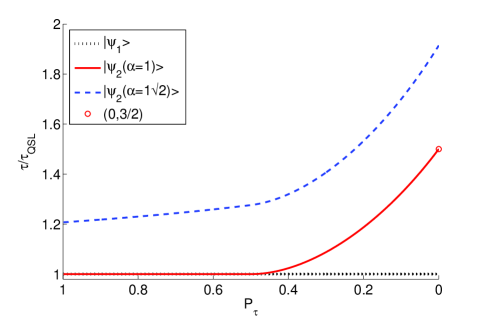
Figure 1: (Color online) Quantum-speed-limit time ratio $\tau_{QSL}/\tau$ of a two-qubit open system under a memoryless environment as a function of $P_{\tau}$ with initial states $\left|\Psi_{1}\right\rangle=\alpha|01\rangle+\sqrt{1-\alpha^{2}}|10\rangle$ (black dotted line), $\left|\Psi_{2}(\alpha=1)\right\rangle=|11\rangle$ (red solid curve), and $\left|\Psi_{2}(\alpha=1/\sqrt{2})\right\rangle=$ $(|11\rangle+|00\rangle)/\sqrt{2}$ (blue dashed curve). The red circle indicates the maximal speedup of quantum evolution for state $\left|\Psi_{2}(\alpha=1)\right\rangle=|11\rangle.$

Obviously, the QSL time ratio $\tau_{QSL}$ of state $\left|\Psi_{1}\right\rangle$ is the same as the exact form in single qubit cases discovered in Refs QSLopen3 ; Xu1 , where the reduction in QSL time ($\tau/\tau_{QSL}>1$) only occurs when the environment is of memory; otherwise the evolution will always be along the QSL time ($\tau/\tau_{QSL}\equiv 1$). In order to illustrate this phenomenon clearly, the QSL time ratio $\tau/\tau_{QSL}$ of initial state $\left|\Psi_{1}\right\rangle$ (black dotted line) is depicted in Fig. 1 under a memoryless environment, i.e., $\left|\overset{\cdot}{P}_{t}\right|=-\overset{\cdot}{P}_{t}$ with the population $P_{t}$ monotonically decreasing from 1 to the target $P_{\tau}$.

However, a complex but interesting phenomenon appears for initial state $\left|\Psi_{2}\right\rangle$: QSL reduction can also take place even when the environment is of no memory. For instances, $\tau/\tau_{QSL}$ versus $P_{\tau}$ of initial states $\left|\Psi_{2}(\alpha=1)\right\rangle=|11\rangle$ (red solid curve) and $\left|\Psi_{2}(\alpha=1/\sqrt{2})\right\rangle=$ $(|11\rangle+|00\rangle)/\sqrt{2}$ (blue dashed curve) are depicted, respectively, in Fig. 1, where $\tau/\tau_{QSL}\geq 1$ clearly illustrates the intrinsic acceleration potential of quantum evolution under a memoryless environment. Especially, there exists a sudden change point in QSL time with the critical point $P_{\tau}=1/2$ for initial state $\left|\Psi_{2}(\alpha=1)\right\rangle=$ $|11\rangle$. To explain this phenomenon, we trace back to $||L_{t}\rho_{t}||_{\infty}$ defined in Eq. (1) with the following expression

$$||L_{t}\rho_{t}||_{\infty}=\left\{\begin{array}[]{l}-\overset{\cdot}{P}_{t}(2\alpha^{2}P_{t}-\alpha^{2}+\alpha),\\ \overset{\cdot}{P}_{t}(2\alpha^{2}P_{t}-\alpha^{2}-\alpha),\end{array}\right.\begin{array}[]{c}P_{t}\geqslant\frac{1}{2},\\ P_{t}<\frac{1}{2},\end{array}$$ (7)

where we have employed the condition of memoryless environment $\left|\overset{\cdot}{P}_{t}\right|=-\overset{\cdot}{P}.$ Therefore, the QSL time ratio $\tau/\tau_{QSL}$ of Eq. (6) can be conveniently calculated as

$$\frac{\tau}{\tau_{QSL}}=\left\{\begin{array}[]{ll}\frac{1+\alpha P_{\tau}}{\alpha(1+P_{\tau})},&P_{\tau}\geqslant\frac{1}{2},\\ \frac{2(1-P_{\tau})(1-\alpha P_{\tau})+\alpha}{2\alpha(1-P_{\tau}^{2})}&P_{\tau}<\frac{1}{2}.\end{array}\right.$$ (8)

One may check that $\tau/\tau_{QSL}\geq 1$ is always satisfied. In particular, when the initial state is in $\Psi_{2}(\alpha=1)=|11\rangle$, the QSL time ratio yields

$$\frac{\tau}{\tau_{QSL}}=\left\{\begin{array}[]{ll}1,&P_{\tau}\geqslant\frac{1}{2},\\ \frac{2(1-P_{\tau})^{2}+1}{2(1-P_{\tau}^{2})}&P_{\tau}<\frac{1}{2}.\end{array}\right.$$ (9)

The sudden change point of QSL time is therefore justified.

II.2 Three-qubit cases

In this subsection, we also consider two typical three-qubit states, i.e., W type state $\left|\Psi_{3}\right\rangle=\alpha|001\rangle+\beta|010\rangle+\sqrt{1-\alpha^{2}-\beta^{2}}|100\rangle$ and GHZ type state $\left|\Psi_{4}\right\rangle=\alpha|111\rangle+\sqrt{1-\alpha^{2}}|000\rangle.$ According to Eq. (1), the expressions of the QSL time ratio are obtained:

$$\frac{\tau}{\tau_{QSL}}=\frac{\int_{0}^{\tau}\left|\overset{\cdot}{P}_{t}\right|dt}{1-P_{\tau}}$$ (10)

for state $\left|\Psi_{3}\right\rangle$ and

$$\frac{\tau}{\tau_{QSL}}=\frac{\int_{0}^{\tau}\max\left\{\left|\overset{\cdot}{P}_{t}(\pm\frac{3}{2}X+3\alpha P_{t}-\frac{3}{2}\alpha)\right|\right\}dt}{\alpha+\alpha(1-\alpha^{2})P_{\tau}(3-2P_{\tau}^{\frac{1}{2}}-3P_{\tau})+\alpha(2\alpha^{2}-1)P_{\tau}^{3}},$$ (11)

for state $\left|\Psi_{4}\right\rangle$, where $X=(4\alpha^{2}P_{t}^{4}-8\alpha^{2}P_{t}^{3}+8\alpha^{2}P_{t}^{2}-5\alpha^{2}P_{t}+P_{t}+\alpha^{2})^{\frac{1}{2}}.$

Equation (10) bears a resemblance to the case of state $\left|\Psi_{1}\right\rangle$, implying that the reduction in QSL only occurs in a memory environment. As for Eq. (11), we consider a special case, i.e., $\left|\Psi_{4}(\alpha=1)\right\rangle=|111\rangle$ under the environment of no memory ($\left|\overset{\cdot}{P}_{t}\right|=-\overset{\cdot}{P}$). Therefore, the Eq. (11) can be simplified as:

$$\frac{\tau}{\tau_{QSL}}=\left\{\begin{array}[]{ll}1,&P_{\tau}\geqslant\frac{1}{2},\\ \frac{(-3P_{\tau}+3P_{\tau}^{2}-P_{\tau}^{3}+\frac{7}{4})}{1-P_{\tau}^{3}}&P_{\tau}<\frac{1}{2},\end{array}\right.$$ (12)

indicating that there also exists a sudden transition of speedup potential of quantum evolution even the environment is of no memory.

II.3 N-qubit cases

In this subsection, we show that the above phenomena are ubiquitous in n-qubit cases (n is an arbitrary positive integer). It is easy to check that if the n-qubit open system is initially prepared in state $\alpha_{1}\left|100\cdots 0\right\rangle+\alpha_{2}\left|010\cdots 0\right\rangle+\cdots+\alpha_{N}\left|000\cdots 1\right\rangle,$ with $\sum_{j=1}^{N}\alpha_{j}^{2}=1,$ the QSL ratio is exactly the same as Eqs. (5) and (10). Therefore, the memory effect of environment becomes the essential condition for the speedup potential emerge in quantum evolution.

However, if the initial state is in $\left|11\cdots 1\right\rangle$, the QSL ratio is given by

$$\frac{\tau}{\tau_{QSL}}=\left\{\begin{array}[]{ll}1,&P_{\tau}\geqslant\frac{1}{2},\\ \frac{\int_{0}^{\tau}\max\{|n\overset{\cdot}{P}_{t}P_{t}^{n-1}|,|-n\overset{\cdot}{P}_{t}(1-P_{t})^{n-1}|\}dt}{1-P_{\tau}^{n}}&P_{\tau}<\frac{1}{2}.\end{array}\right.$$ (13)

In particular when the environment is memoryless, i.e., $\left|\overset{\cdot}{P}_{t}\right|=-\overset{\cdot}{P},$ Eq. (13) reduces to

$$\frac{\tau}{\tau_{QSL}}=\left\{\begin{array}[]{ll}1,&P_{\tau}\geqslant\frac{1}{2},\\ \frac{(1-P_{\tau})^{n}+1-(\frac{1}{2})^{n-1}}{1-P_{\tau}^{n}}&P_{\tau}<\frac{1}{2}.\end{array}\right.$$ (14)

Clearly, $P_{\tau}=1/2$ is the critical point at which the open system experiences the sudden change of QSL time under a memoryless environment.

Equation (14) also implies that there exists a maximal acceleration potential condition for state $\left|11\cdots 1\right\rangle$ when $P_{\tau}\rightarrow 0$, and the corresponding minimal QSL time ratio is given by:

$$\frac{\tau}{\tau_{QSL}}|_{\max}=\frac{2^{n}-1}{2^{n-1}}.$$ (15)

Especially when $n=2$, Eq. (15) grows to $3/2$, which is marked in Fig. 1 as the red circle.

II.4 Memory effect on QSL time

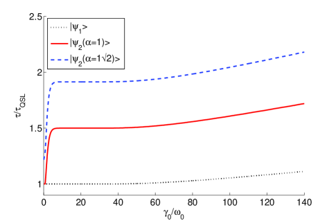
Figure 2: (Color online) Quantum-speed-limit time $\tau_{QSL}$ of a Lorentzian spectral distribution model versus coupling strength $\gamma_{0}.$ The black dotted, red solid, and blue dashed curves represent the two-qubit initial states $\left|\Psi_{1}\right\rangle=\alpha|01\rangle+\sqrt{1-\alpha^{2}}|10\rangle$, $\left|\Psi_{2}(\alpha=1)\right\rangle=|11\rangle$, and $\left|\Psi_{2}(\alpha=1/\sqrt{2})\right\rangle=$ $(|11\rangle+|00\rangle)/\sqrt{2}$, respectively, with parameters $\lambda=50$, $\omega_{0}=1$, and $\tau=1.$

In this subsection, we intend to show that memory effect of environment is still an important element for quantum acceleration potential for multi-qubit open systems. The memory environment we consider here is characterized by the Lorentzian spectral distribution $J(\omega)=\frac{1}{2\pi}\frac{\gamma_{0}\lambda}{(\omega_{0}-\omega)^{2}+\lambda^{2}}$ , where $\gamma_{0}$ is the Markovian decay rate and $\lambda$ is the spectral width Book Open . $P_{t}$ is now written as Book Open

$$P_{t}=e^{-\lambda t}\left|\cosh(\frac{dt}{2})+\frac{\lambda}{d}\sinh(\frac{dt}{2})\right|^{2},$$ (16)

where $d=\sqrt{2\gamma_{0}\lambda-\lambda^{2}}$. In Fig. 2, we take two-qubit initial states as an example and fix the driving time as $\tau=1.$The QSL time ratio $\tau/\tau_{QSL}$ versus coupling strength $\gamma_{0}/\omega_{0}$ is plotted with three typical two-qubit states $\left|\Psi_{1}\right\rangle$ (black dotted line), $\left|\Psi_{2}(\alpha=1)\right\rangle$ (red solid curve), and $\left|\Psi_{2}(\alpha=1/\sqrt{2})\right\rangle$ (blue dashed curve), respectively, with $\lambda=50$, $\omega_{0}=1$, and we set $\tau_{QSL}=1$. According to Ref. (Book Open ), we know that $\gamma_{0}=\lambda/2$ is the transient point from memoryless environment ($\gamma_{0}<\lambda/2$) to one of memory ($\gamma_{0}>\lambda/2$). As is clearly shown in Fig. 2, more capacity for potential speedup will take place when the environment enters the memory region.

III Discussion: Entanglement and QSL time

Considering that the QSL time for multiqubit systems can be shortened in a memoryless environment, it is natural to link this phenomenon to entanglement, which only exists in multiqubit cases. In closed composite systems, entanglement has been taken as a resource in the speedup of quantum evolution [c5 ; en2 ; en3 ; en4 ]. In this subsection, we go a step further to the connection between entanglement and QSL time in bipartite open systems. The initial state we consider here is an arbitrary pure state:

$$\left|\phi\right\rangle=\alpha_{1}|11\rangle+\alpha_{2}|10\rangle+\alpha_{3}|01\rangle+\alpha_{4}|00\rangle,$$ (17)

with $\sum_{j=1}^{4}\alpha_{j}{}^{2}=1,$ which is generated by Monte Carlo method, and the related entanglement is characterized by concurrence $C$ in Ref. concurrence , with $C=0$ for a disentangled state and $C=1$ for a maximally entangled state.

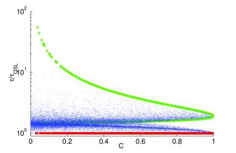
Figure 3: (Color online) Quantum speed limit time ratio $\tau_{QSL}/\tau$ as a distribution of concurrence $C$ for 20000 randomly generated initial pure states (tiny blue dots) under the damping model. The dark red and light green dots represent QSL time ratio with states $\left|\Psi_{1}\right\rangle=\alpha|01\rangle+\sqrt{1-\alpha^{2}}|10\rangle$ and $\left|\Psi_{2}\right\rangle=\alpha|11\rangle+\sqrt{1-\alpha^{2}}|00\rangle,$ respectively.

In Fig. 3, 20000 random pure states are generated by Monte Carlo sampling new3 and their QSL ratios $\tau/\tau_{QSL}$ and their QSL time ratios $\tau/\tau_{QSL}$ under memoryless environments versus concurrence are marked by tiny blue dots. As is clearly displayed in Fig. 3, the lower bound $\tau/\tau_{QSL}=1$ can always be reached by states $\left|\Psi_{1}\right\rangle=\alpha|01\rangle+\sqrt{1-\alpha^{2}}|10\rangle$ (dark red dots in Fig. 3), implying that the concurrence has nothing to do with $\tau/\tau_{QSL}$ under this circumstance. In addition, the upper bound is taken by a subset of states $\left|\Psi_{2}\right\rangle=\alpha|11\rangle+\sqrt{1-\alpha^{2}}|00\rangle$ (light green dots in Fig. 3), illustrating that weak entanglement may reduce the QSL time more.

We also note that, if one takes the viewpoint of Scenario 1, the upper subset of light green dots in Fig. 3 implies that entanglement is able to accelerate quantum evolution under such a circumstance.

IV Conclusion

In summary, we have explored the quantum-speed-limit time for multi-qubit open systems. For a certain class of initial states, we have demonstrated that the quantum evolution can also be accelerated in a memoryless (Markovian) environment. Moreover, we have found that entanglement plays a subtle role in the speedup of quantum evolution: weak entanglement may be better for speeding up quantum evolution under certain circumstances.

We have only treated non-correlated environments in this paper. It will also be of importance and interest to study the QSL time of multi-qubit systems with the presence of initial correlations among the subsystems of composite environments EML .

V Acknowledgement

This work was supported by the National Natural Science Foundation of China (Grants No. 11204196 and No. 11074184), the Specialized Research Fund for the Doctoral Program of Higher Education (Grant No. 20123201120004), and the Priority Academic Program Development of Jiangsu Higher Education Institutions.

References

- (1) L. Mandelstam and I. Tamm, J. Phys. (USSR) 9, 249 (1945).
- (2) N. Margolus and L. B. Levitin, Phys. D 120, 188(1998).
- (3) S. Lloyd, Nature (London) 406, 1047 (2000).
- (4) T. Caneva, M. Murphy, T. Calarco, R. Fazio, S. Montangero, V. Giovannetti, and G. E. Santoro, Phys. Rev. Lett. 103, 240501 (2009).
- (5) G. C. Hegerfeldt, Phys. Rev. Lett. 111, 260501 (2013).
- (6) V. Mukherjee, A. Carlini, A. Mari, T. Caneva, S. Montangero, T. Calarco, R. Fazio, and V. Giovannetti, Phys. Rev. A 88, 062326 (2013).
- (7) G. C. Hegerfeldt, Phys. Rev. A 90, 032110 (2014).
- (8) S. Deffner, J. Phys. B 47, 145502 (2014).
- (9) V. Giovanetti, S. Lloyd, and L. Maccone, Nature Photonics 5, 222 (2011).
- (10) A. W. Chin, S. F. Huelga, and M. B. Plenio, Phys. Rev. Lett. 109, 233601 (2012).
- (11) M. Tsang, New J. Phys. 15 073005 (2013).
- (12) S. Deffner and E. Lutz, Phys. Rev. Lett. 105, 170402 (2010).
- (13) G. N. Fleming, Nuovo Cimento A 16, 232 (1973).
- (14) J. Anandan and Y. Aharonov, Phys. Rev. Lett. 65, 1697 (1990).
- (15) L. Vaidman, Am. J. Phys. 60, 182 (1992).
- (16) P. Pfeifer and J. Frohlich, Rev. Mod. Phys. 67, 759 (1995).
- (17) V. Giovannetti, S. Lloyd, and L. Maccone, Phys. Rev. A 67, 052109 (2003).
- (18) S. Luo, Phys. D 189, 1 (2004).
- (19) S. Luo, J. Phys. A 38, 1991 (2005).
- (20) L. B. Levitin and T. Toffoli, Phys. Rev. Lett. 103, 160502 (2009).
- (21) S. Fu, N. Li, and S. Luo, Commun. Theor. Phys 54, 661 (2010).
- (22) P. J. Jones and P. Kok, Phys. Rev. A 82, 022107 (2010).
- (23) M. Zwierz, Phys. Rev. A 86, 016101 (2012).
- (24) S. Deffner and E. Lutz, J. Phys. A 46, 335302 (2013).
- (25) B. Russell and S. Stepney, Phys. Rev. A 90, 012303 (2014).
- (26) A. Carlini, A. Hosoya, T. Koike, and Y. Okudaira, J. Phys. A 41, 045303 (2008).
- (27) A.-S. F. Obada, D. A. M. Abo-Kahla, N. Metwally, M. Abdel-Aty, Physica E 43, 1792 (2011).
- (28) M. M. Taddei, B. M. Escher, L. Davidovich, and R. L. de Matos-Filho, Phys. Rev. Lett. 110, 050402 (2013).
- (29) A. del Campo, I. L. Egusquiza, M. B. Plenio, and S. F. Huelga, Phys. Rev. Lett. 110, 050403 (2013).
- (30) S. Deffner and E. Lutz, Phys. Rev. Lett. 111, 010402 (2013).
- (31) C. L. Latune, B. M. Escher, R. L. de Matos Filho, and L. Davidovich, Phys. Rev. A 88, 042112 (2013).
- (32) Z.-Y. Xu, S. Luo, W. L. Yang, C. Liu, and S. Zhu, Phys. Rev. A 89, 012307 (2014).
- (33) Z.-Y. Xu and S. Zhu, Chin. Phys. Lett. 31, 020301 (2014).
- (34) J. Batle, M. Casas, A. Plastino, and A. R. Plastino, Phys. Rev. A 72, 032337 (2005).
- (35) A. Borras, M. Casas, A. R. Plastino, and A. Plastino, Phys Rev. A 74, 022326 (2006).
- (36) F. Frowis, Phys. Rev. A 85, 052127 (2012).
- (37) H.-P. Breuer, J. Phys. B 45, 154001 (2012).
- (38) Á. Rivas, S. F. Huelga, and M. B. Plenio, Rep. Prog. Phys. 77 094001 (2014).
- (39) B. Bellomo, R. Lo Franco, and G. Compagno, Phys. Rev. Lett. 99, 160502 (2007).
- (40) H.-P. Breuer and F. Petruccione, The Theory of Open Quantum Systems (Oxford University Press, Oxford, 2007).
- (41) G. Toth, Comput. Phys. Commun. 179, 430 (2008).
- (42) W. K. Wootters, Phys. Rev. Lett. 80, 2245 (1998).
- (43) E.-M. Laine, H.-P. Breuer, J. Piilo, C.-F. Li, and G.-C. Guo, Phys. Rev. Lett. 108, 210402 (2012).