The frequency and the structure of large character sums
Abstract.
Let denote the maximum of for a given non-principal Dirichlet character , and let denote a point at which the maximum is attained. In this article we study the distribution of as one varies over characters (mod ), where is prime, and investigate the location of . We show that the distribution of converges weakly to a universal distribution , uniformly throughout most of the possible range, and get (doubly exponential decay) estimates for ’s tail. Almost all for which is large are odd characters that are -pretentious. Now, , and one knows how often the latter expression is large, which has been how earlier lower bounds on were mostly proved. We show, though, that for most with large, is bounded away from , and the value of is little bit larger than .
Key words and phrases:
Distribution of character sums, distribution of Dirichlet -functions, pretentious multiplicative functions, random multiplicative functions2010 Mathematics Subject Classification:
Primary: 11N60. Secondary: 11K41, 11L401. Introduction
For a given non-principal Dirichlet character , where is an odd prime, let
This quantity plays a fundamental role in many areas of number theory, from modular arithmetic to -functions. Our goal in this paper is to understand how often is large, and to gain insight into the structure of those characters for which is large.
It makes sense to renormalize by defining
and we believe that
| (1.1) |
where is the Euler–Mascheroni constant. Rényi [Rén47] observed that with
Upper bounds on (and hence on ) have a rich history. The 1919 Pólya–Vinogradov Theorem states that
for all non-principal characters . Apart from some improvements on the implicit constant [Hil88, GS07], this remains the state-of-the-art for the general non-principal character, and any improvement of this bound would have immediate consequences for other number theoretic questions (see e.g. [BG16]). Montgomery and Vaughan [MV77] (as improved in [GS07]) have shown that the Generalized Riemann Hypothesis implies
whereas, for every prime , there are characters for which
(see [BC50, GS07], which improve on Paley [Pal]), so the conjectured upper bound (1.1) is the best one could hope for. However, for the vast majority of the characters , is somewhat smaller, and so we study the distribution function
Montgomery and Vaughan [MV79] showed that for all for any fixed (they equivalently phrase this in terms of the moments of ). This was recently improved by Bober and Goldmakher [BG13], who proved that, for fixed and as through the primes,
| (1.2) |
where is some positive constant and
| (1.3) |
and is the modified Bessel function of the first kind given by
| (1.4) |
We improve upon these results and demonstrate that decays in a double exponential fashion:
Theorem 1.1.
Let . If is a prime number, and for some , then
where
The proof implies that of the characters for which are odd, so it makes sense to consider odd and even characters separately. Hence we define
| (1.5) |
We outline the proof of Theorem 1.1 in Section 4, and fill in the details in subsequent sections. The range of uniformity barely misses implying the upper bound in (1.1); even so, it does show that is rarely large. Calculations reveal that each tend to a universal distribution function , and we will show this for later on. In Figure 1 we graph for a typical :
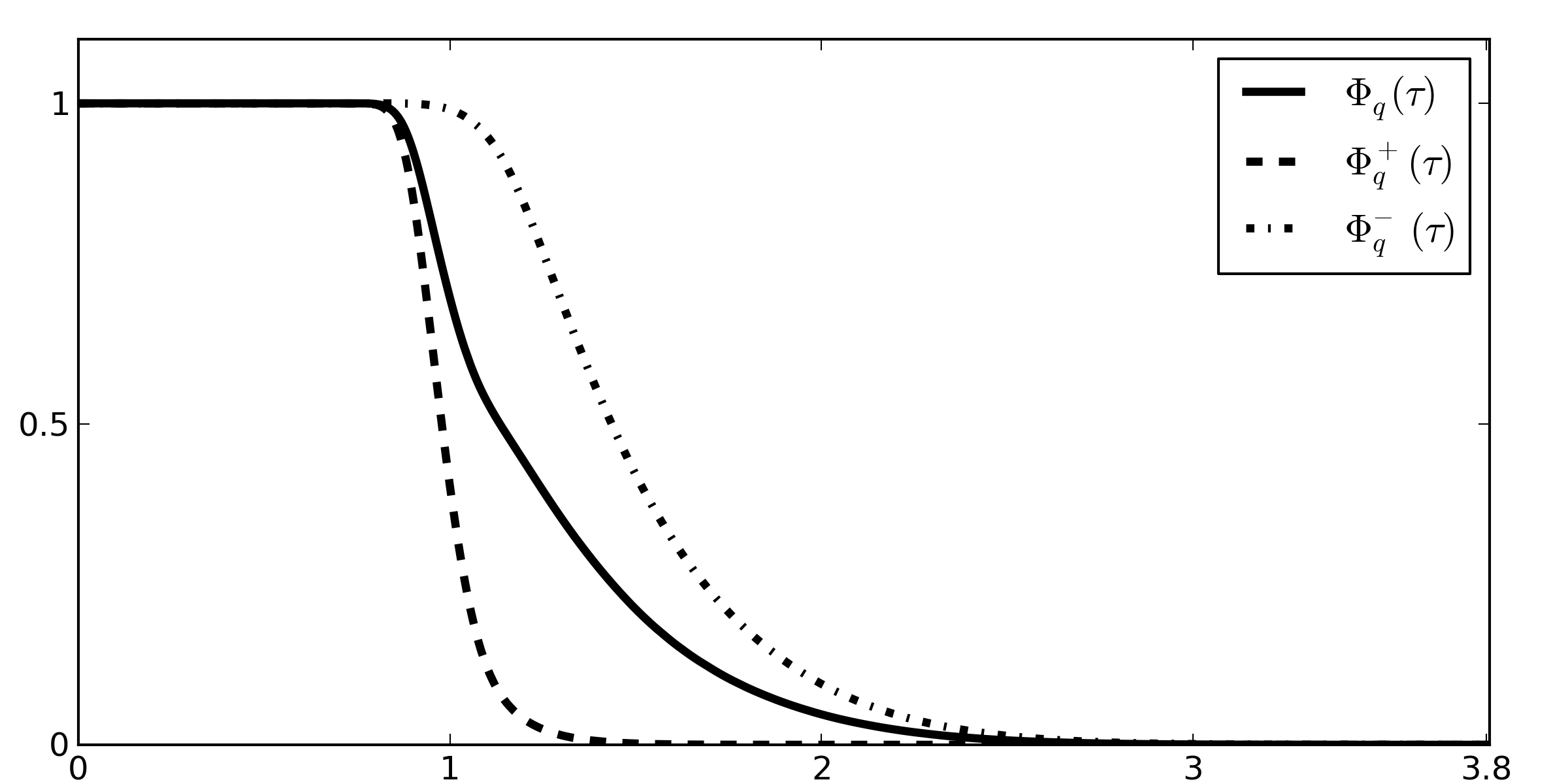
Notice that for all , and then it decays quickly: and . For more computational data, the reader is invited to consult Table 1 in Section 10.
The distribution of , for prime, decays similarly [GS06]:
| (1.6) |
with , uniformly for , . This similarity is no accident, since for an odd, non-primitive character , the average of the character sum is
where is the Gauss sum, so that . In particular, if is large, then so is . Moreover, for as above, we have the pointwise formula
which implies that
a little larger than if . The distribution of can be analyzed in the same way as the distribution of . However, even if , then we can show that the average of our character sum up to is slightly larger than when is close to . This builds on ideas in [Bob14].
Theorem 1.2.
Let be an odd prime, for a sufficiently large absolute constant . There exists a subset of cardinality
| (1.7) |
such that if and is sufficiently large, then
| (1.8) |
We can deduce that
This result, together with (1.6), suggests that the lower bound in Theorem 1.1 should be sharp, and that when these quantities are “large”. However the numerical evidence indicates that is perhaps typically a little bigger:
The numerical comparison between and (the -distribution for odd characters ) is given in Figure 3:
Even characters
The focus above has been on odd characters since almost all characters with are odd. However, we can obtain analogous results for even characters.
Theorem 1.3.
There exists an absolute constant such that if is an odd prime and for some , then
The lower bound in the above theorem has the same shape as (1.6) and it might be close to the truth, unlike the corresponding result for (as explained by Theorem 1.2). This is supported by computations, as it can be seen in Figure 4.
The distribution function
Classically, the statistical behavior of as varies over all non-principal characters mod is modelled by , where the are independent random variables, each uniformly distributed on the unit circle , and for . This suggests modelling , , by . Indeed, in [GS03] this was shown to be a very successful model. Similarly, one might guess that the distribution of could be accurately modelled by (and thus by ), but this seems unlikely since, for fixed , we have that
as . Moreover Harper [Har13] recently showed that is not normally distributed, and subsequently we have no idea what its distribution should be (though [CS12] shows that is normally distributed provided is not too large).
So, what is the right way to model ? One reason the above model failed is that it does not take account of characters’ periodicity. The periodicity of , via the formula
where , leads to Pólya’s formula [MV07, eqn. (9.19), p. 311]:
| (1.9) |
(which is periodic for ). Since , this suggests modelling by the random variable
where is a random variable independent of the ’s, with probability 1/2 of being or , and we have set . The infinite sum here converges with probability 1,111This follows by the methods of Section 5 applied to in place of . so that is well defined, and we can consider its distribution function,
The following result confirms our intuition that serves as a good model for .
Theorem 1.4.
If and is continuous at every point of , then the sequence of functions converges to uniformly on . In particular, the sequence of distributions converges weakly to .
Acknowledgements
The authors would like to thank Sandro Bettin, Adam Harper, K. Soundararajan, Akshay Venkatesh, John Voight, and Trevor Wooley for some helpful discussions. AG and DK are partially supported by Discovery Grants from the Natural Sciences and Engineering Research Council of Canada.
Notation
Given a positive integer , we let and be the largest and smallest prime divisors of , with the notational convention that and . Furthermore, we write for the set of integers all of whose prime factors lie in . The symbol denotes the number of ways can be written as a product of positive integers. We denote with the number of distinct primes that divide , and with the total number of prime factors of , counting multiplicity. Finally, we use the symbol to indicate the characteristic function of the set . For example, equals 1 if and 0 otherwise.
2. The structure of characters with large
We now determine more precise information about the structure of characters with large .
Theorem 2.1.
Let be an odd prime and for a sufficiently large absolute constant . There exists a set of cardinality
| (2.1) |
for which the following holds: If , then
-
(1)
is an odd character.
-
(2)
Let , and be the reduced fraction for which with . Let if is prime, and otherwise. Then
(2.2) (2.3)
Granville and Soundararajan showed in [GS07] that if is large then must pretend to be a character of small conductor and of opposite parity (that is, is “-pretentious”). Building on the techniques of [GS07], Theorem 2.2 shows that, for the vast majority of characters with large , the character is the trivial character, and must be odd (and so -pretentious as in (2.2)).
Inequality (2.2) allows us to establish accurate estimates for for all . Here and for the rest of the paper, for we set
| (2.4) |
where is the Dickman–de Bruijn function, defined by for and via the differential-delay equation for . Then we have the following estimate:
Theorem 2.2.
Let and be as in Theorem 2.1. Given , let be the reduced fraction for which with . Define by .
-
(a)
If , then
-
(b)
If , then
where
Moreover, if we take and write , then we have that
Notice that if then , so is a measure of the distance between and .
Theorems 2.1 and 2.2 will be proved in Section 9. Analogous results can also be proven for even characters:
Theorem 2.3.
Let be an odd prime and for a sufficiently large constant . There exists a set of cardinality
| (2.5) |
for which the following statements hold. If then
-
(1)
If , and is the reduced fraction for which with , then .
-
(2)
We have that
(2.6) (2.7) -
(3)
Given , let be the reduced fraction for which with . Define by . Then
3. Auxiliary results about smooth numbers
Before we get started with the proofs of our main results, we state and prove some facts about smooth numbers. As usual, we set
We begin with the following simple estimates.
Lemma 3.1.
For , we have that
Proof.
Lemma 3.2.
For and , we have that
Proof.
We also need the following result, where is defined by (2.4).
Lemma 3.3.
If and , then
In particular, .
Proof.
Remark 3.1.
Using the slightly more accurate approximation
for (see [Sai89]), one can similarly deduce the stronger estimate
for all .
Finally, we have the following key estimate. Its second part is a strengthening of Theorem 11 in [FT91].
Lemma 3.4.
Let and .
-
(a)
We have that
-
(b)
There is an absolute constant such that if , is a reduced fraction with and , then
where is defined by and is von Mangoldt’s function.
Proof.
(a) If , then , and so
Hence it suffices to show that
| (3.3) |
Note that if , then
using partial summation on the estimate . Therefore, in order to complete the proof of (3.3), it suffices to show that
where . Moreover, Lemma 3.2 reduces the above relation to showing that
| (3.4) |
where . In particular, we may assume that . If , then Theorem 10 in [FT91] and relation (3.2) imply that
provided that , for sufficiently large. (This lower bound on guarantees that the parameter in Theorem 10 of [FT91] is , as required.) Consequently, if we set , then partial summation implies that
Then (3.4) follows from
| (3.5) |
which is trivial unless , so that .
Let for . Let be the largest integer for which . Then . If for some and , then Theorem 3 in [Hil86] implies that
Therefore, partial summation and Lemma 3.1 imply that
Summing the above relation over and bounding trivially the contribution of implies that
Finally, integration by parts gives us that
by the definition of and Lemma 3.1. This completes the proof of (3.5) and thus the proof of part (a) of the lemma.
(b) Write and set . We note that, since , by assumption, we must have that .
We start by estimating the part of the sum with . We claim that
| (3.6) |
Note that if , then
by partial summation and the estimate . Therefore, it suffices to prove that
where . Furthermore, Lemma 3.2 reduces the above estimate to showing that
| (3.7) |
where . For this sum to have any summands we need that .
Next, we fix and estimate
for . Let be the constant in Theorem 10 of [FT91] when the parameters and there equal 100 and , respectively, and set and . There is some reduced fraction with and . Note that
In particular, we must have that . If, in addition, , then Theorem 11 in [FT91] and relation (3.2) imply that
where . Therefore
| (3.8) |
if .
Consider now such that and set . We claim that . We argue by contradiction: assume, instead, that . Then and thus and . In particular, and thus , which implies that , a contradiction.
Using the above information, we are going to show that
| (3.9) |
when . If this relation holds, then (3.7) follows by a straightforward dyadic decomposition argument. We use the stronger relation (3.8) for the dyadic intervals corresponding to , and we use (3.9) for the dyadic intervals with .
It remains to prove (3.9) when , in which case lies in the interval . In addition, note that . Let for . Let be the largest integer for which . Then . Consider for some and set . Since , Theorems 2 and 5 in [FT91] imply that
since (see, for example, Lemma 7.6 below). Note that
for . Therefore
| (3.10) |
We apply Theorem 3 in [Hil86] to find that
for and . Consequently,
for some constant . Since , applying partial summation as in the proof of part (a), we deduce that
Setting , summing the above relation over , and bounding trivially the contribution of implies that
Finally, we have that
whence
To conclude, we have shown that
Since , we further deduce that
Observe that
| (3.11) |
where denotes the distance of from its nearest integer. Note that by our assumption that . Since we also have that , a consequence of the fact that , the error term in (3.11) is
by our assumption that . Hence, the lemma is reduced to showing that
By Lemma 3.2, it suffices to show that
| (3.12) |
where . Since , the argument leading to (3.10) implies that
for . Therefore partial summation yields
Arguing as in Lemma 3.3, we apply partial summation on relation (3.1) to deduce that
Consequently,
since and by Lemma 3.1. This completes the proof of (3.12) and thus the proof of the lemma. ∎
Corollary 3.5.
Let be a Dirichlet character modulo and . For all , we have
Proof.
If is an even character, then , so that
by the Prime Number Theorem, as desired. We may therefore assume that is an odd character, so that
If , where is the constant from Lemma 3.4(b), then Lemma 3.4(a) implies that
which is admissible. Finally, assume that , and consider a reduced fraction with and . Then Lemma 3.4(b) and the Prime Number Theorem imply that
where . Since and , we deduce that
which concludes the proof. ∎
4. Outline of the proofs of Theorems 1.1 and 1.3 and proof of Theorem 1.2
We first deal with Theorem 1.3. For the lower bound, note that if is even and , then [MV07, eqn. (9.18), p. 310] yields the inequality
Since we also have that
| (4.1) |
we deduce that
for all even characters . The lower bound in Theorem 1.3 is a direct consequence of the above inequality and of the following result, whose proof is a straightforward application of the methods in [GS07]:
Theorem 4.1 (Granville - Soundararajan).
If is a character modulo some , is the set of odd or of even characters mod , and for some , then
Finally, the upper bound in Theorem 1.3 follows from Theorems 4.1 and 2.3. (The proof of the latter theorem is independent of the proof of the upper bound of Theorem 1.3, as we will see.)
Next, we turn to Theorem 1.1. Its lower bound is a direct consequence of Theorems 1.2 and 4.1. So it remains to outline the proof of the upper bound in Theorem 1.1, as well as to prove Theorem 1.2. In the heart of these two proofs lies a moment estimate which implies that the bulk of the contribution in Pólya’s Fourier expansion (1.9) comes from smooth inputs:
for most and any . To state this more precisely, we need some notation. Given a set of positive integers , set
in the special case when , write in place of . Observe that
| (4.2) |
Our next goal is to show that is small for most . To do this, we will prove in Section 5 that high moments of are small. As a straightforward application of our moment bounds we will get the following theorem.
Theorem 4.2.
If , and , then
Proof of the upper bound in Theorem 1.1.
We conclude this section with the proof of Theorem 1.2.
Proof.
The set in which we work is defined by
where we have set for some constant . If the constant in the statement of Theorem 1.2 is large enough, then Theorems 4.2 and 4.1 imply that (1.7) does hold.
Assume now that . Using partial summation on the Pólya–Vinogradov inequality, then that , and finally Lemma 3.2, we obtain
| (4.3) |
Given that , we deduce that
| (4.4) |
by Mertens’s estimate. Therefore
Taking logarithms, we find that
that is, is “-pretentious”. Since for , the above inequality and the Cauchy–Schwarz inequality imply that
| (4.5) |
for all . Moreover, since
we find that
| (4.6) |
Now, since is odd for , Pólya’s Fourier expansion (1.9) implies that
| (4.7) |
Set
If and is sufficiently large, then Lemma 3.4 and relation (4.7) imply that
Now, Lemma 3.2 and relation (4.6) yield that
for some complex numbers of modulus . Finally, if , then we simply note the trivial bound , which follows by our assumption that for the we are working with. So (1.8) will certainly follow if we show that
By Cauchy–Schwarz, it suffices to show that
| (4.8) |
For convenience, set , and note that
where
Therefore
Note that
and
Using the bound , we conclude that
Since for , (4.8) follows. This completes the proof of (1.8).
5. Truncating Pólya’s Fourier expansion
In this section we show that for most we can limit the Fourier expansion to a sum over very smooth numbers without much loss, which is the content of Theorem 4.2. We prove this theorem by showing that high moments of are small:
Theorem 5.1.
Let and be integers with . For , we have that
One consequence of Theorem 5.1 is the desired conclusion that is usually small:
Deduction of Theorem 4.2 from Theorem 5.1.
We may assume that and are large. Let be the proportion of characters such that . Moreover, set
where is a constant to be determined. Then Theorem 5.1 implies that
which completes the proof. ∎
We prove Theorem 5.1 as an application of the following technical estimates.
Proposition 5.2.
Let and be two integers with , and , where and are two positive real numbers such that . Then
Proposition 5.3.
Let and be two integers with , and , where and are two positive real numbers such that . Then
Before we proceed to the proof of these propositions, let us see how we can apply them to deduce Theorem 5.1.
Deduction of Theorem 5.1 from Propositions 5.2 and 5.3.
Set . Then
where is the set of integers all of whose prime factors lie in . We let
so that
| (5.1) |
We shall bound the moments of each summand appearing above, individually.
We start with the summand involving . Here we may assume that (and thus ), else and so for all . Set and note that
by Lemma 3.2. So Minkowski’s inequality and Proposition 5.3 imply that
Hence, applying Hölder’s inequality and Mertens’ estimate , we arrive at the estimate
| (5.2) |
Next, in order to bound the summand in (5.1) involving , we observe that
for all by Proposition 5.2. Therefore Hölder’s inequality implies that
| (5.3) |
Finally, relations (5.1), (5.2) and (5.3), together with an application of Minkowski’s inequality, imply that
| (5.4) |
We note that, for all , we have that
| (5.5) |
Indeed, if , then , whereas if , then . Combining (5.4) and (5.5) completes the proof of Theorem 5.1. ∎
Our next task is to show Proposition 5.2. First, we demonstrate the following auxiliary lemma.
Lemma 5.4.
Let and be an integer. Uniformly for and for , we have that
Proof.
Proof of Proposition 5.2.
Without loss of generality, we may assume that is large, else the result is trivially true. Set , so that
Hölder’s inequality with and implies that
| (5.6) |
which reduces the problem to bounding
for . In order to do this, we first decouple the , the point where the maximum occurs, from the character . We accomplish this by noticing that for every and for every , there is some such that . Then
We choose . Then Minkowski’s inequality implies that
| (5.7) |
which reduces Proposition 5.2 to bounding
Notice that
| (5.8) |
where
Clearly,
So opening the square in (5.8), and summing over , we find that
| (5.9) |
The right hand side of (5.9) is at most , where
We shall bound each of these sums in a different way.
Next, we bound . Note that for and in the support of . In particular, for to have any summands, we need that . We choose such that
| (5.11) |
Then
| (5.12) |
Our goal is to bound
for every that is coprime to . First, assume that . Note that is supported on integers which can be written as a product with each of the factors lying in the interval and having all their prime factors . In particular, for all and consequently
by (5.11). In particular,
by our assumptions that and that . This inequality also holds when , since in this case for all and for the numbers in the range of . So, no matter what is, we conclude that
| (5.13) |
since . Inserting (5.13) into (5.12), we arrive at the estimate
| (5.14) |
Combining relations (5.10) and (5.14) with (5.9), we deduce that
Together with (5.7), the above estimate implies that
since we have assumed that . Together with (5.6), this implies that
Since and , Proposition 5.2 follows. ∎
Proof of Proposition 5.3.
Without loss of generality, we may assume that is large enough. We start in a similar way as in the proof of Proposition 5.2: we set and note that
Therefore, Minkowski’s inequality implies that
We claim that
| (5.15) |
for all . Proposition 5.3 follows immediately if we show this relation, since we would then have that
by our assumption that and (5.5), which establishes Proposition 5.3.
Arguing as in the proof of Proposition 5.2 and setting
we find that
| (5.16) |
where
We shall bound each of these sums in a different way.
We start with bounding . Set
for large enough , so that . Also, let . Fix with , and note that if with , then . Therefore
| (5.17) |
We fix as above, set for all , and choose such that
| (5.18) |
Then, for any that is coprime to , the Cauchy–Schwarz inequality implies that
So, applying Lemma 5.4, we deduce that
since and , by (5.18). Inserting this estimate into (5.17), we deduce that
| (5.19) |
Consequently, we immediately deduce that
| (5.20) |
which is admissible.
It remains to bound . This will be done in a very different way. We observe that if are the random variables defined in the introduction, then
We have that
where
Therefore
by Minkowski’s inequality. Fix . When , then , whereas if , then we use the trivial bound , for any . Therefore
We have that
since and by the Prime Number Theorem. Moreover,
as and , with . Choosing for an appropriate small constant makes the left hand side for some . We take to conclude that
where we used our assumption that is large and . We thus conclude that
by (5.5). Together with (5.16) and (5.20), this completes the proof of relation (5.15) and, thus, of Proposition 5.3. ∎
6. The distribution function
In this section, we prove Theorem 1.4. Throughout this section we fix and a large odd prime number such that . Set and
Relation (4.2) and Lemma 3.2 imply that
Therefore, if is large enough, then Theorem 4.2 and Lemma 3.2 imply that
where the last relation follows by Theorem 1.1 and our assumption that . Therefore we conclude that
where
| (6.1) |
We perform the same analysis on . With a slight abuse of notation, we set
The analogue of Theorem 4.2 for the random variables is (more easily) proven by the same method with a few simple changes: we proceed exactly as in the proof of Theorem 5.1 but wherever we evaluated a sum there (as , unless when it equals ), we now evaluate an expectation which equals unless , when it equals . (In fact this only happens in the proofs of (5.9) and of (5.16).) We then conclude that
| (6.2) |
where
(We could have written in place of in (6.2) but this would have required proving a lower bound for . In order to avoid this technical issue, we use for comparison whose size we already know by Theorem 1.1.) Next, for each we fix a parameter of the form with to be chosen, and a partition of the unit circle into arcs of length . Moreover, we let be the point in the middle of the arc and we define to be the set of -tuples with and for all primes . Given such a choice of and , we set and . Moreover, similarly to before, we let
We will show that there exist choices of and a constant such that if and belongs to the arc centred at for all , then . This immediately implies that
| (6.3) |
where
It remains to show that if is chosen appropriately. We choose these parameters so that . Then the condition that for each prime implies that for all with . Hence
which proves our claim.
We now prove similar inequalities for , namely that
| (6.4) |
Theorem 9.3 of [Lam08] states that if is an arc of length for each , then
The same methods can easily be adapted to also show that
for . Since , the inequality is indeed satisfied for our choice of , thus completing the proof of (6.4).
Finally, combining relations (6.1), (6.2), (6.3) and (6.4), we obtain
If is continuous in , then it is also uniformly continuous. It then follows immediately from the above estimate that as over primes, uniformly on . In order to see that converges also weakly to , consider a continuous function of bounded support. Fix . Since has at most countable many discontinuity points, we deduce that there is an open set of Lebesgue measure that contains all discontinuities of . If is a bounded closed interval containing the support of , then the set is compact and thus it can be written as a finite union of closed intervals. Since converges uniformly to on each such interval, it does so on as well. Therefore
Since was arbitrary, we conclude that
thus completing the proof of Theorem 1.4.
7. Some pretentious results
In this section, we develop some general tools we will use to prove Theorems 2.1 and 2.3. We begin by stating a result that allows us to concentrate on the case when is a rational number with a relatively small denominator.
Lemma 7.1.
Let , , be a Dirichlet character, and . Let be a reduced fraction with and . Then
where .
Proof.
When is large, we have the following result.
Lemma 7.2.
Let , where . For all , we have that
Proof.
For smaller , we shall use the following formula.
Lemma 7.3.
Let be a Dirichlet character and . For we have that
Proof.
If , then
So, writing for the greatest common divisor of and , we find that
Finally, observe that the innermost sum vanishes if is an even character, whereas if is odd it equals
This concludes the proof of the lemma. ∎
Following Granville and Soundararajan [GS07], we are going to show that the all the terms in the right hand side in Lemma 7.3 are small unless is induced by some fixed character which depends at most on and . As in [GS07], in order to accomplish this, we define a certain kind of “distance” between two multiplicative functions and of modulus :
Then we let be a primitive character of conductor such that
| (7.1) |
We need a preliminary result on certain sums of multiplicative functions, which is the second part of Lemma 4.3 in [GS07].
Lemma 7.4.
Let be a multiplicative function. For we have that
Then we have the following “repulsion” result.
Lemma 7.5.
Let , and be as above. If is a Dirichlet character modulo , of conductor , that is not induced by , then
Proof.
When applying Lemma 7.3, we will need to evaluate the Gauss sum that arises. In order to do this, we shall use the following classical result (see, for example, Theorem 9.10 in [MV07, p. 289]).
Lemma 7.6.
Let be a character modulo induced by the primitive character modulo . Then
We also need the following simple estimate, which we state below for easy reference.
Lemma 7.7.
Let be a completely multiplicative function. For all , we have that
and
Proof.
We write if for all primes . Then
The second part is proved similarly, starting from the identity
Combining the above results, we prove the following simplified version of Lemma 7.3.
Lemma 7.8.
Let , , and be as above, and consider a real number and a reduced fraction with and . If either or is even, then
whereas if and is odd, then
Proof.
By Lemma 7.5, we see that if is a character modulo that is not induced by , then
| (7.2) |
So the first result follows by Lemma 7.3. Finally, if and is odd, then Lemmas 7.3 and 7.6, and (7.2) imply that
Writing , noticing that if , and using the trivial bound
to extend the sum over to a sum over , we find that
Setting and applying Lemma 7.7 with and in place of we deduce that
Since we have assumed that , we have that
| (7.3) |
If with , then
Therefore the absolute value of the sum in (7.3) is
Since we also have that , we deduce that
where we used Lemma 7.4 and the inequality for . This completes the proof of the lemma. ∎
Finally, if pretends to be 1 in a strong way, then we can get a very precise estimate on the sum of over smooth number using estimates for such numbers in arithmetic progressions due to Fouvry and Tenenbaum [FT91].
Lemma 7.9.
Let , be a character mod , and be a reduced fraction with . Then
where is the largest divisor of with and , with
Proof.
First, note that the inequality follows by the Cauchy–Schwarz inequality and the fact that for . We write . Then we have that and thus
| (7.4) |
Moreover, observe that, using Lemma 3.2, we may assume that .
We begin by estimating the sum
for . Set and note that
| (7.5) |
where we bounded trivially the sum over when (note that for all ).
Next, we need an estimate for the sum
when . Note that, since , Theorems 2 and 5 in [FT91] imply that
when ; the same result also holds when by elementary techniques since for and . So, using the identity
we deduce that
where we used (7.4). We get the same right side no matter what the value of , as long as . Hence
for some function satisfying the bound
Letting , and writing and so that , we deduce that
by [Dav00, eq (7), p. 149], for all . Therefore partial summation implies that
Integrating by parts and applying relation (7.4) and our assumption that we conclude that
Since we also have that
we deduce that
| (7.6) |
Applying Lemma 7.7 with and in place of implies that
Inserting this formula into (7.6) leads to an error term of size
and a main term of
times
thus completing the proof of the lemma. ∎
Corollary 7.10.
Let be an integer that either equals 1 or is prime. Let , and be a reduced fraction with . Then
8. Structure of even characters with large : proof of Theorem 2.3
The goal of this section is to prove Theorem 2.3. Throughout this section, we set for some constant . We will show this theorem with
where the quantity is defined as in Section 4. Theorem 4.2 and the lower bound in Theorem 1.3, which we already proved in the beginning of Section 4 (independently of the proof of Theorem 2.3), guarantee that the cardinality of satisfies (2.5), provided that the constant in the definition of and the constant in the statement of Theorem 2.3 are large enough.
We fix a large and we consider a character . Let . Then
by (1.9), our assumption that for , and Lemma 3.2. As in the statement of Theorem 2.3, we approximate by a reduced fraction with and . We let and apply Lemma 7.1 with to find that
| (8.1) |
Since , we must have that , which implies that
| (8.2) |
We now proceed to show that satisfies properties (1) and (2) of Theorem 2.3.
Proof of Theorem 2.3 - Property (1).
Firstly, note that Lemma 7.2 in conjunction with (8.2) implies that . Equation (8.2) also tells us that we must be in the second case of Lemma 7.8 (provided that is large enough), that is to say and is odd. Since is even, we conclude that is odd. Thus . Moreover, the last inequality in Lemma 7.8 implies that
Comparing this inequality with (8.2), we deduce that and thus , the quadratic character modulo 3, which completes the proof of our claim and hence of the fact that Property (1) holds. ∎
Proof of Theorem 2.3 - Property (2).
We start with the proof of (2.7). Note that
where . Then using (4.1), we find that
so that, by (8.1),
Hence, we conclude that
Therefore
which, in turn, implies that
so that
| (8.4) |
Finally, we have that
by the Pólya–Vinogradov inequality, our assumption that and Lemma 3.2. Inserting the above estimates into (8.4) completes the proof of (2.7).
Proof of Theorem 2.3 - Property (3).
Define via the relation . Note that as . So we may show the theorem with in place of . Arguing as at the beginning of Section 8, and applying Lemma 7.1 with , we find that
We note that inequality (8.5) and the argument leading to (4.6) imply that
| (8.6) |
where we have set . We write with , so that
by (8.6) and as . Using the formula , we deduce that
If is not a power of 3, then for each , so Corollary 7.10 implies that
as claimed. Finally, if and , then , unless and , so that . Therefore Corollary 7.10 and Lemma 3.3 imply that
This completes the proof of Theorem 2.3. ∎
9. The structure of characters with large : proof of Theorems 2.1 and 2.2
The goal of this section is to prove Theorems 2.1 and 2.2. Throughout this section, we set for some constant (note that this a different value of than in the previous section). We will show this theorem with
where the quantity is defined as in Section 4. Theorem 4.2 and the lower bound in Theorem 1.1, which we already proved in the beginning of Section 4, guarantee that the cardinality of satisfies (2.1), provided that the constant in the definition of and the constant in the statement of Theorem 2.1 are large enough.
We fix a large and we consider a character . Let be such that
As in the statement of Theorem 2.1, we pick a reduced fraction such that and , and we define to equal if is prime, and 1 otherwise. Following the argument leading to (8.1), we deduce that
| (9.1) |
where .
Proof of Theorem 2.1 - Property (1).
We choose with to satisfy (7.1). Since , we must have that , which implies that
| (9.2) |
We claim that
| (9.3) |
the first relation being Property (1). We separate two cases.
First, assume that . Then we apply Lemma 7.2 to find that
which, together with (9.2), implies that
| (9.4) |
Then we must have that . Furthermore, the first part of Lemma 7.8 implies that and thus . Finally, Lemma 7.4 and (9.4) imply that , which completes the proof of (9.3) in this case.
Finally, assume that . Suppose that either is even or . Then Lemma 7.8 implies that
So (9.2) becomes
| (9.5) |
Thus we must be in the second case of Lemma 7.8 as far as the above sum is concerned, that is to say that and is odd. Then the second part of Lemma 7.8 implies that
Comparing this inequality with (9.5), we deduce that and thus , provided that is large enough. But then has to be odd, which contradicts our initial assumption. So we conclude that our initial assumption must be wrong, that is to say must be odd and , so that .
In order to prove Property (2) in Theorem 2.1, we need an intermediate result: we set
for , and
as in Lemma 7.9, where we used (9.3). Additionally, we set
and we write , where
The intermediate result we need to show is that
| (9.6) |
Before proving this, we show how to use it to complete the proof of Theorem 2.1.
Proof of Theorem 2.1 - Property (2).
We argue as in the proof of Property (2) in Theorem 2.3. For (2.3), note that our assumption that implies, as , that, for all ,
Therefore,
for all , by the Pólya–Vinogradov inequality, and Lemma 3.2. So (2.3) follows from (9.6) but with the weaker error term in place of , where if , and otherwise, so that . We argue much like we did getting to to (4.5): We have
so that
and therefore
This implies that
In particular, , so that we always have that and . This completes the proof of Property (2) in Theorem 2.1. ∎
Proof of (9.6).
We separate two main cases.
Case 1. Assume that . Then (9.1) and the fact that is odd imply that
| (9.7) |
Since , we find that
Consequently, , which in turn gives us that . Inserting this estimate into (9.7), we deduce that
that is to say, (9.6) holds (with a stronger error term).
Case 2. Assume that . Then (9.1) and Lemma 7.9 implies that
Now Lemma 7.7, applied with and in place of , implies that
| (9.8) |
So, if we set
| (9.9) |
then we have that
| (9.10) |
Our goal is to show, using formula (9.10), that for all . Indeed, if this were true, then . We start by observing that
| (9.11) |
Indeed, reversing the last steps of the proof of Lemma 7.9, we find that
Moreover,
Combining the two above relations, we obtain (9.11).
Using (9.11) and the inequality , we deduce that
| (9.12) |
for . Inserting this into (9.10), and since
we obtain that
| (9.13) |
We also have
by Lemma 7.7. Together with (9.13), this implies that
Since this holds as an upper bound too, we deduce that
| (9.14) |
Substituting (9.14) into (9.13) we obtain
| (9.15) |
and then comparing (9.13) with the displayed line above,
| (9.16) |
where we have set for .
Case 2a. Assume that has at least two distinct prime factors. If , then we can find two distinct primes and such that with , , and (which only fails for or ). Therefore, taking absolute values in (9.9), we find that
Note that
| (9.17) |
Therefore
Now when so that, for and ,
since and . We therefore deduce that
Now , and so
and therefore, by (9.9),
Substituting this into (9.10), and using (9.8), yields (9.6) in this case, except if .
When , we use relations (9.11) and (9.17) to deduce that
Since the left hand side is and , we deduce that , as before. Proceeding now as in the case completes the proof (9.6) when too.
Case 2b. Now suppose that is a prime power with . Using (9.11), we see that
Define so that and . Then
which is and by (9.12) and (9.16). Taking real parts, and noting that each Re, we deduce that Re Re by considering the and terms. Hence
and therefore
Substituting this into (9.10), and using (9.8), yields the result in this case.
Case 2c. Now suppose that is a prime, so that . Hence we cannot use (9.16) to gain information on . Now, using Lemma 7.7, we have
Combining this with (9.14) yields that ; that is
Taking real parts, we deduce that
with the lower bound being trivial. This implies that
Using Lemma 7.7, we then conclude that
which, together with (9.10), completes the proof of (9.6) in this last case too. ∎
Remark 9.1.
Note that can be quite big if is small and if is not very close to . So we cannot say more than the last formula without more information on the location of .
We conclude the paper with the proof of Theorem 2.2.
Proof of Theorem 2.2.
Let for a large enough constant , as above, and define via the relation . Note that . So we may show the theorem with in place of . Arguing as at the beginning of this section, and applying Lemma 7.1 with , we find that
Note that (2.2) and the argument leading to (4.6) imply that
| (9.18) |
for all . Hence is -pretentious.
Now suppose that . Substituting (9.18) in our formula for , we obtain
If , then we bound the second sum using Corollary 7.10. If , then the result follows from Lemma 3.3. This concludes the proof of part (a).
Finally, assume that is a prime number so that . Writing with , we find that
by (9.18) and the trivial estimate . If , then we have that
by Lemmas 7.7 and 3.3. Next, if for all , then for all . So Corollary 7.10 implies that
as claimed. Finally, assume that for some . The terms with contribute
by Lemmas 7.7 and 3.3. When , we apply Corollary 7.10. The total contribution of those terms is
by Lemmas 7.7 and 3.3. Putting the above estimates together, yields the estimate
with . To finish the proof of the theorem, we specialize the above formula when , in which case , so that . Then the modulus of the left hand side equals , which is by assumption. On the other hand, if we set , then
Consequently,
Since and , we have that
Putting together the above inequalities proves the last claim of part (b). Hence the proof of Theorem 2.2 is now complete. ∎
10. Additional tables
| even | odd | all | ||||||||||
|---|---|---|---|---|---|---|---|---|---|---|---|---|
| min | mean | max | min | mean | max | mean | ||||||
| 10000019 | 0.728 | 0.994 | 1.74 | 2.11 | 0.788 | 1.51 | 3.35 | 3.74 | 1.25 | 3.25 | ||
| 10000079 | 0.725 | 0.994 | 1.75 | 2.05 | 0.795 | 1.51 | 3.35 | 3.81 | 1.25 | 3.26 | ||
| 10000103 | 0.725 | 0.994 | 1.75 | 2 | 0.793 | 1.51 | 3.34 | 3.83 | 1.25 | 3.25 | ||
| 10000121 | 0.724 | 0.994 | 1.75 | 2.02 | 0.793 | 1.51 | 3.34 | 3.78 | 1.25 | 3.26 | ||
| 10000139 | 0.726 | 0.994 | 1.75 | 2.01 | 0.797 | 1.51 | 3.35 | 3.74 | 1.25 | 3.25 | ||
| 10000141 | 0.719 | 0.994 | 1.74 | 2.02 | 0.79 | 1.51 | 3.33 | 3.82 | 1.25 | 3.25 | ||
| 10000169 | 0.721 | 0.994 | 1.75 | 2.06 | 0.788 | 1.51 | 3.34 | 3.73 | 1.25 | 3.25 | ||
| 10000189 | 0.709 | 0.994 | 1.75 | 2.01 | 0.793 | 1.51 | 3.35 | 3.71 | 1.25 | 3.25 | ||
| 10000223 | 0.73 | 0.994 | 1.75 | 2 | 0.783 | 1.51 | 3.34 | 3.81 | 1.25 | 3.25 | ||
| 10000229 | 0.723 | 0.994 | 1.74 | 2.04 | 0.784 | 1.51 | 3.33 | 3.79 | 1.25 | 3.25 | ||
| 10000247 | 0.716 | 0.994 | 1.74 | 2.05 | 0.794 | 1.51 | 3.34 | 3.71 | 1.25 | 3.25 | ||
| 10000253 | 0.724 | 0.994 | 1.75 | 2.05 | 0.783 | 1.51 | 3.34 | 3.75 | 1.25 | 3.25 | ||
| 11000027 | 0.724 | 0.994 | 1.75 | 2.03 | 0.797 | 1.51 | 3.34 | 3.72 | 1.25 | 3.25 | ||
| 11000053 | 0.733 | 0.994 | 1.75 | 2.07 | 0.781 | 1.51 | 3.34 | 3.81 | 1.25 | 3.25 | ||
| 11000057 | 0.707 | 0.994 | 1.75 | 2.03 | 0.79 | 1.51 | 3.34 | 3.74 | 1.25 | 3.25 | ||
| 11000081 | 0.724 | 0.994 | 1.75 | 2.01 | 0.789 | 1.51 | 3.33 | 3.77 | 1.25 | 3.25 | ||
| 11000083 | 0.724 | 0.994 | 1.75 | 2.05 | 0.799 | 1.51 | 3.34 | 3.84 | 1.25 | 3.25 | ||
| 11000089 | 0.728 | 0.994 | 1.75 | 2.05 | 0.794 | 1.51 | 3.33 | 3.77 | 1.25 | 3.26 | ||
| 11000111 | 0.724 | 0.994 | 1.75 | 2.03 | 0.796 | 1.51 | 3.33 | 3.72 | 1.25 | 3.26 | ||
| 11000113 | 0.719 | 0.994 | 1.75 | 2.01 | 0.781 | 1.51 | 3.34 | 3.73 | 1.25 | 3.25 | ||
| 11000149 | 0.731 | 0.994 | 1.75 | 2.03 | 0.805 | 1.51 | 3.34 | 3.72 | 1.25 | 3.25 | ||
| 11000159 | 0.722 | 0.994 | 1.75 | 2 | 0.797 | 1.51 | 3.33 | 3.83 | 1.25 | 3.25 | ||
| 11000179 | 0.724 | 0.994 | 1.74 | 2.03 | 0.796 | 1.51 | 3.35 | 3.86 | 1.25 | 3.26 | ||
| 11000189 | 0.728 | 0.994 | 1.75 | 2.1 | 0.794 | 1.51 | 3.34 | 3.68 | 1.25 | 3.26 | ||
| 12000017 | 0.723 | 0.994 | 1.74 | 2.08 | 0.8 | 1.51 | 3.34 | 3.8 | 1.25 | 3.26 | ||
| 12000029 | 0.72 | 0.994 | 1.74 | 2.06 | 0.791 | 1.51 | 3.33 | 3.84 | 1.25 | 3.26 | ||
| 12000073 | 0.735 | 0.994 | 1.75 | 2.05 | 0.794 | 1.51 | 3.34 | 3.9 | 1.25 | 3.26 | ||
| 12000091 | 0.728 | 0.994 | 1.75 | 2.02 | 0.794 | 1.51 | 3.35 | 3.73 | 1.25 | 3.26 | ||
| 12000097 | 0.719 | 0.994 | 1.75 | 2.08 | 0.788 | 1.51 | 3.34 | 3.75 | 1.25 | 3.25 | ||
| 12000127 | 0.724 | 0.994 | 1.75 | 2.09 | 0.794 | 1.51 | 3.34 | 3.71 | 1.25 | 3.25 | ||
| 12000133 | 0.727 | 0.994 | 1.75 | 2.11 | 0.785 | 1.51 | 3.34 | 3.73 | 1.25 | 3.25 | ||
| 12000239 | 0.715 | 0.994 | 1.75 | 2.02 | 0.797 | 1.51 | 3.34 | 3.8 | 1.25 | 3.25 | ||
| 12000253 | 0.713 | 0.994 | 1.75 | 2.02 | 0.786 | 1.51 | 3.34 | 3.76 | 1.25 | 3.26 | ||
References
- [BC50] P. T. Bateman and S. Chowla, Averages of character sums. Proc. Amer. Math. Soc. 1 (1950), 781–787.
- [BG13] J. Bober and L. Goldmakher, The distribution of the maximum of character sums. Mathematika 59 (2013), no. 2, 427–442.
- [BG16] by same author, Pólya–Vinogradov and the least quadratic nonresidue. Math. Ann. 366 (2016), no. 1-2, 853–863.
- [Bob14] J. Bober, Averages of character sums. Preprint (2014). arXiv:1409.1840
- [CS12] S. Chatterjee and K. Soundararajan, Random multiplicative functions in short intervals. Int. Math. Res. Not. IMRN (2012), no. 3, 479–492.
- [Dav00] H. Davenport, Multiplicative number theory. Third edition. Revised and with a preface by Hugh L. Montgomery. Graduate Texts in Mathematics, 74. Springer-Verlag, New York, 2000.
- [dB51] N. G. de Bruijn, On the number of positive integers and free of prime factors . Nederl. Acad. Wetensch. Proc. Ser. A. 54 (1951), 50–60.
- [DE52] H. Davenport and P. Erdős, The distribution of quadratic and higher residues. Publ. Math. Debrecen 2 (1952), 252–265.
- [FT91] É. Fouvry and G. Tenenbaum, Entiers sans grand facteur premier en progressions arithmétiques. Proc. London Math. Soc. (3) 63 (1991), no. 3, 449–494.
- [Gol12] L. Goldmakher, Multiplicative mimicry and improvements to the Pólya–Vinogradov inequality. Algebra Number Theory 6 (2012), no. 1, 123–163.
- [GS03] A. Granville and K. Soundararajan, Distribution of values of . Geom. Funct. Anal. 13 (2003), no. 5., 992–1028.
- [GS06] by same author, Extreme values of . The Riemann zeta function and related themes: papers in honour of Professor K. Ramachandra, 65–80, Ramanujan Math. Soc. Lect. Notes Ser., 2, Ramanujan Math. Soc., Mysore, 2006.
- [GS07] by same author, Large character sums: pretentious characters and the Pólya–Vinogradov theorem. J. Amer. Math. Soc. 20 (2007), no. 2, 357–384.
- [Har13] A. J. Harper, On the limit distributions of some sums of a random multiplicative function. J. Reine Angew. Math. 678 (2013), 95–124.
- [Hil86] A. Hildebrand, On the number of positive integers and free of prime factors . J. Number Theory 22 (1986), no. 3, 289–307.
- [Hil88] by same author, Large values of character sums. J. Number Theory 29 (1988), no. 3, 271–296.
- [HT93] A. Hildebrand and G. Tenenbaum. Integers without large prime factors. J. Théor. Nombres Bordeaux 5 (1993), no. 2, 411–484.
- [Lam08] Y. Lamzouri, The two-dimensional distribution of values of . Int. Math. Res. Not. IMRN (2008), Vol. 2008, 48 pp. doi:10.1093/imrn/rnn106
- [MV77] H. L. Montgomery and R. C. Vaughan, Exponential sums with multiplicative coefficients. Invent. Math. 43 (1977), no. 1, 69–82.
- [MV79] by same author, Mean values of character sums. Canad. J. Math., 31(3):476–487, 1979.
- [MV07] by same author, Multiplicative number theory. I. Classical theory. Cambridge Studies in Advanced Mathematics, 97. Cambridge University Press, Cambridge, 2007.
- [Pal] R. E. A. C. Paley, A Theorem on Characters. J. London Math. Soc. S1-7 no. 1, 28.
- [Rén47] A. A. Rényi. On some new applications of the method of Academician I. M. Vinogradov. Doklady Akad. Nauk SSSR (N. S.) 56 (1947), 675–678.
- [Sai89] É. Saias, Sur le nombre des entiers sans grand facteur premier. (French) [On the number of integers without large prime factors] J. Number Theory 32 (1989), no. 1, 78–99.
- [Ten95] G. Tenenbaum, Introduction to analytic and probabilistic number theory. Translated from the second French edition (1995) by C. B. Thomas. Cambridge Studies in Advanced Mathematics, 46. Cambridge University Press, Cambridge, 1995.