On the Search for Inhomogeneous Phases in Fermionic Models

Abstract

We revisit the Gross-Neveu model with $N$ fermion flavors in 1+1 dimensions and compute its phase diagram at finite temperature and chemical potential in the large-$N$ limit. To this end, we double the number of fermion degrees of freedom in a specific way which allows us to detect inhomogeneous phases in an efficient manner. We show analytically that this “fermion doubling trick” predicts correctly the position of the boundary between the chirally symmetric phase and the phase with broken chiral symmetry. Most importantly, we find that the emergence of an inhomogeneous ground state is predicted correctly. We critically analyze our approach based on this trick and discuss its applicability to other theories, such as fermionic models in higher dimensions, where it may be used to guide the search for inhomogeneous phases.

I Introduction

The search for exotic phases, such as Fulde-Ferrell-Larkin-Ovchinnikov-type phases Fulde and Ferrell (1964); Larkin and Ovchinnikov (1965), plays an important role in various different fields of physics, ranging from condensed-matter systems (see, e.g., Refs. Jackiw and Schrieffer (1981); Mertsching and Fischbeck (1981); Machida and Nakanishi (1984); Chodos et al. (1999); Kleinert and Babaev (1998)), over ultracold atomic gases (see, e.g., Refs. Bulgac and Forbes (2008); Baarsma and Stoof ; Radzihovsky (2012); Roscher et al. (2014)), to exactly solvable, relativistic model field theories for the strong interaction (see, e.g., Refs. Schon and Thies (2000, ); Schnetz et al. (2004, 2006); Basar and Dunne (2008a, b); Basar et al. (2009)) and high-energy physics with an emphasis on QCD phenomenology (see, e.g., Refs. Bringoltz (2007, 2009); Nickel (2009); Kojo et al. (2010); Buballa and Carignano ), see also Refs. Casalbuoni and Nardulli (2004); Thies (2006) for more general reviews. The latter studies were triggered by Thies’ ground-breaking analyses of inhomogeneous phases in Gross-Neveu type models in $1+1$ dimensions Schon and Thies ; Brzoska and Thies (2002); Thies (2004); Thies and Urlichs (2003).

Loosely speaking, the emergence of condensates in fermionic theories is tightly linked to the formation of bosonic two-fermion bound-states. The macroscopic occupation of the energetically lowest lying bosonic state is then associated with the emergence of a condensate. In general, the latter goes alongside with the spontaneous breakdown of a fundamental symmetry of the underlying fermionic theory, such as the breakdown of the U($1$) symmetry in ultracold Fermi gases indicating the presence of a superfluid ground state. Fulde and Ferrell as well as Larkin and Ovchinnikov suggested that the formation of a spatially varying, i.e. inhomogeneous, ground state might be energetically favored in fermionic systems with two components, provided that the associated Fermi momenta are sufficiently different Fulde and Ferrell (1964); Larkin and Ovchinnikov (1965). The latter can be controlled by, e.g., varying the associated chemical potentials. In such a situation, the energetically lowest lying (bosonic) bound-state configuration may carry a finite center-of-mass momentum. The macroscopic occupation of this state may then give rise to the formation of a spatially varying condensate, see, e.g., Ref. Roscher et al. (2014) for an illustration in the context of ultracold Fermi gases.

For our understanding of the emergence of inhomogeneous phases, studies of – at least within the mean-field approximation – exactly solvable low-dimensional models play a prominent role Schon and Thies ; Thies (2004); Schnetz et al. (2004, 2006); Basar and Dunne (2008a, b); Basar et al. (2009). Noteworthily, in the case of one-dimensional models, the outcomes of mean-field studies are expected to be of most relevance for higher dimensions: Beyond the mean-field approximation, the presence of long-range fluctuations hinders spontaneous symmetry breaking in one dimension Mermin and Wagner (1966); Hohenberg (1967), rendering the results considerably distinct from higher dimensions. Hence, from a field-theoretical point of view, mean-field studies of a given one-dimensional model are rather considered to be useful to guide studies of the corresponding model in three dimensions where fluctuation effects often play a less prominent role. In particular, the above-mentioned knowledge of analytic solutions in the one-dimensional case is very appealing since it allows to provide analytic guidance for, e.g., studies of QCD with imaginary chemical potential Karbstein and Thies (2007) underlying many lattice simulations (see, e.g., Refs. de Forcrand and Philipsen (2002); Lombardo (2006); Philipsen (2013)), and also opens up the possibility to develop and benchmark new techniques for, e.g., the study of the emergence of inhomogeneous phases being the subject of the present study. In the latter case, the techniques may then be applied to models in higher dimensions where the search for the existence of inhomogeneous ground states requires in general the use of numerical methods. Therefore, already one-dimensional models serve as a valuable test ground to better understand how the dynamics of a strongly coupled field theory like, e.g., QCD is affected by the presence of a baryon Schon and Thies ; Schnetz et al. (2004, 2006) or isospin chemical potential Ebert et al. (2011); Gubina et al. (2012); Ebert et al. (2014).

In this paper, we present and discuss a “fermion doubling trick” which allows to search for the emergence of inhomogeneous phases in an efficient way. For illustration purposes, we use this trick to study the phase diagram of the Gross-Neveu (GN) model in one spatial dimension at finite temperature and chemical potential in the large-$N$ limit. We show that the position of the transition line between the chirally symmetric phase and the phase with broken chiral symmetry is recovered correctly for this model, rendering the fermion doubling trick potentially useful to assist the search for inhomogeneous phases in higher dimensional fermionic models. In Sect. II, we introduce our fermion doubling approach and exemplarily demonstrate the computation of the effective potential based thereon for the GN model. Moreover, our approach and its limitations are critically reviewed and discussed. The phase diagram of the GN model as obtained from our doubling approach is presented in Sect. III and compared to the well-known exact solution Thies and Urlichs (2003); Schnetz et al. (2004); Thies (2006). Our conclusions are given in Sect. IV.

II Formalism

II.1 Gross-Neveu Model

In the present work, we refrain from repeating all the well-known attractive features of the GN model but rather highlight the most important features relevant for our study and refer the reader to some pertinent review articles otherwise, see Refs. Schon and Thies ; Feinberg (2004); Thies (2006) and the references therein.

Originally, the GN model has been introduced as a toy model for the strong interaction, and more specifically to study dynamical chiral symmetry breaking in asymptotically free fermionic theories Gross and Neveu (1974). It describes the quantum field theory of $N$ flavors of relativistic fermions interacting via a four-fermion interaction term. Its action in $d=$1+1 Euclidean space-time dimensions reads

$$S=\int_{\tau}\int_{x}\,\Big{\{}\bar{\psi}\left({\rm i}\not{\partial}+{\rm i}\mu\gamma_{0}\right)\psi+\frac{g^{2}}{2}\left(\bar{\psi}\psi\right)^{2}\Big{\}}\,,$$ (1)

where $\int_{\tau}\equiv\int_{0}^{\beta}d\tau$, $\int_{x}\equiv\int dx$, $\beta=1/T$ is the inverse temperature, and $\mu$ is the chemical potential.

We tacitly assume that the field $\psi$ in Eq. (1) is built up of $N$ two-component spinors, $\psi^{T}=(\psi_{1},\dots,\psi_{N})$, with the lower index labeling the $N$ flavors. Our Euclidean conventions for the Dirac $\gamma$-matrices are

$$\gamma_{0}=\begin{pmatrix}0&1\\ 1&0\end{pmatrix}\,,\qquad\text{and}\qquad\gamma_{1}=\begin{pmatrix}0&-{\rm i}\\ {\rm i}&0\end{pmatrix}\,,$$ (2)

with $\{\gamma_{\mu},\gamma_{\nu}\}=2\delta_{\mu\nu}\mathbb{1}_{2\times 2}$ and $\gamma_{5}={\rm i}\gamma_{0}\gamma_{1}$.

In $d=1+1$, the GN model is perturbatively renormalizable and asymptotically free. The coupling $g$ is dimensionless and represents a marginally relevant parameter at the Gaußian fixed point. Since we do not account for a bare fermion mass in the present study, the value of any dimensionful physical quantity $\mathcal{O}$ only depends on our choice for the value of the coupling $g$ at a given UV momentum scale $\Lambda$. This implies that all physical observables are uniquely fixed by our choice for the coupling. Here, we choose the physical fermion mass $M_{0}$ at vanishing temperature and chemical potential to set the scale. Dimensionless ratios $\mathcal{O}/M_{0}$ are then given by universal numbers, i.e. they are independent of our actual choice for $g$.

The action (1) of the GN model is invariant under global U$(N)$ transformations of the fermion fields, implying that the associated U($1$) charge is conserved for each flavor separately. It is also invariant under discrete $\mathbb{Z}_{2}$ chiral transformations:

$$\bar{\psi}\mapsto-\bar{\psi}\gamma_{5}\,,\qquad\psi\mapsto\gamma_{5}\psi\,{,}$$ (3)

implying that $\bar{\psi}\psi\mapsto-\bar{\psi}\psi$. However, the infrared regime (long-range limit) of the theory is governed by dynamical chiral symmetry breaking, independent of our choice for the coupling $g$, see also below.

The chiral symmetry of the model can be associated with a $\mathbb{Z}_{2}$ symmetry of the scalar order parameter $\langle\bar{\psi}\psi\rangle$. To see this explicitly, it is convenient to introduce a real-valued auxiliary scalar field $\sigma$ into the path integral representation of the partition function ${\mathcal{Z}}$,

$${\mathcal{Z}}=\int{\mathcal{D}}\bar{\psi}{\mathcal{D}}\psi\,{\rm e}^{-S}\,,$$ (4)

by means of a Hubbard-Stratonovich transformation Hubbard (1959); Stratonovich (1957). Formally, this is done by multiplying ${\mathcal{Z}}$ with a suitably chosen Gaußian factor,

$$1={\mathcal{N}}\int{{\mathcal{D}}\sigma}\,{\rm e}^{-\frac{1}{2g^{2}}\int_{\tau}\int_{x}\sigma^{2}}\,,$$ (5)

where $\mathcal{N}$ is a normalization factor, and then shifting the auxiliary field as follows:

$$\sigma\mapsto\sigma+{\rm i}g^{2}(\bar{\psi}\psi)\,.$$ (6)

The field $\sigma$ carries the same quantum numbers as the composite field $\bar{\psi}\psi$. Its equation of motion is trivially given by $\sigma=-{\rm i}(\bar{\psi}\psi)$, such that obviously $\sigma\mapsto-\sigma$ under discrete chiral $\mathbb{Z}_{2}$ transformations.

Employing Eqs. (5) and (6), the action in Eq. (4) changes as $S\mapsto S_{\rm B}$, with the associated so-called partially bosonized action of the GN model given by

$$S_{\rm B}=\int_{\tau}\int_{x}\,\Big{\{}\bar{\psi}\left({\rm i}\not{\partial}+{\rm i}\sigma+{\rm i}\mu\gamma_{0}\right)\psi+\frac{1}{2g^{2}}\sigma^{2}\Big{\}}\,.$$ (7)

As the fermion fields appear only bilinearly in the action, they can be integrated out exactly, leaving us with a highly non-local purely bosonic effective action, see also our discussion below.

Subsequently, we shall split up the $\sigma$ field into a background field $\bar{\sigma}\equiv\langle\sigma\rangle$ and a fluctuation field, $\sigma\mapsto\bar{\sigma}+\sigma$. The action $S_{\rm B}$ can then be expanded in powers of the bosonic fluctuation field. As we are only interested in a study of the large-$N$ limit here, it suffices to restrict ourselves to the zeroth order of this expansion, i.e., to simply substitute $\sigma$ with $\bar{\sigma}$. Diagrammatically, within the framework of the partially bosonized theory (7), this means that Feynman diagrams with internal boson lines are not taken into account. Higher orders in an expansion of the fluctuation field $\sigma$ are suppressed parametrically by powers of $1/N$ Pausch et al. (1991). The associated Feynman diagrams contain at least one internal boson line.

It is then apparent that the action (7) with $\sigma\mapsto\bar{\sigma}$ is invariant under the discrete $\mathbb{Z}_{2}$ chiral transformations (3) for $\bar{\sigma}=0$, but not for $\bar{\sigma}\neq 0$, confirming that $\bar{\sigma}$ and thus also $\langle\bar{\psi}\psi\rangle$ constitutes an order parameter for chiral symmetry breaking.

II.2 Fermion Doubling

Let us now discuss our fermion doubling approach. To this end, we discuss the computation of the effective order-parameter potential of the GN model in the large-$N$ limit and show that our approach allows us to search for the emergence of inhomogeneous phases in an efficient way.

For our study, it is convenient to switch to momentum space by using the Fourier representation of the fermion fields:

$$\psi(x) = \sum_{n}\int_{p}e^{-{\rm i}(\nu_{n}\tau+px)}\psi_{n}(p)\,,$$ (8)

$$\bar{\psi}(x) = \sum_{n}\int_{p}e^{{\rm i}(\nu_{n}\tau+px)}\bar{\psi}_{n}(p)\,,$$ (9)

where $\int_{p}\equiv\int\frac{dp}{2\pi}$ and $\nu_{n}=(2n+1)\pi T$ are the fermionic Matsubara frequencies. For the real-valued background field $\bar{\sigma}$, we employ the following ansatz:

$$\bar{\sigma}(x)=M\cos(2Qx)=\frac{M}{2}\left(e^{2{\rm i}Qx}+e^{-2{\rm i}Qx}\right)\,.$$ (10)

Here, $M\geq 0$ and $Q$ are real-valued parameters. Chiral symmetry breaking is associated with a ground-state configuration with finite $M$. If the ground-state configuration assumes a finite value $Q$, then translation invariance is broken spontaneously. Thus, $Q$ can be viewed as an order-parameter for translation symmetry breaking. A priori, both types of symmetry breaking are not related.

We add that the ansatz (10) corresponds to an inhomogeneity of the Larkin-Ovchinnikov-type and includes the case of a homogeneous ground state in the limit $Q\to 0$. In many-body physics, the quantity $Q$ can be related to the center-of-mass momentum of the two-body bound-state associated with condensation.

Our ansatz for $\bar{\sigma}$ shares important properties with the analytic solution in the large-$N$ limit: In Refs. Thies and Urlichs (2003); Schnetz et al. (2004), it was indeed shown that the true inhomogeneous ground state is described by a periodic function. At finite temperature close to the chiral phase boundary, it was moreover found that the functional form of the ground state configuration approaches a single cosine of the form (10). For small temperatures, on the other hand, our ansatz for $\bar{\sigma}$ is expected to become insufficient. In fact, the ground-state solution in the zero-temperature limit is given by a kink-antikink crystal Brzoska and Thies (2002); Thies (2004); Thies and Urlichs (2003); Schnetz et al. (2004), also denoted as baryon crystal, which can obviously not be described by a simple single-cosine ansatz.

Inserting our ansatz (10) into the action (7) yields the following expression:

$$S_{\rm B}[\bar{\sigma}]=\Delta S_{\rm B}+\frac{1}{2g^{2}}\int_{\tau}\int_{x}\bar{\sigma}^{2}\,,$$ (11)

with

$$\!\!\!\!\!\Delta S_{\rm B} = \beta\sum_{n}\int_{p}\Big{\{}\bar{\psi}_{n}(p)\left(\nu_{n}\gamma_{0}+p\gamma_{1}+{\rm i}\mu\gamma_{0}\right)\psi_{n}(p)$$ (12)

$$\!\!\!\!\!\!\!\!+\,\frac{M}{2}\left(\bar{\psi}_{n}(p\!+\!2Q)\psi_{n}(p)+\bar{\psi}_{n}(p\!-\!2Q)\psi_{n}(p)\right)\!\Big{\}}\,{.}$$

Focussing on the momentum structure, we observe that the action can be rewritten as follows:

$$\Delta S_{\rm B} = \frac{\beta}{2}\sum_{n}\int_{p}\Big{\{}\bar{\psi}_{n}(p-Q)\gamma_{0}\left(\nu_{n}+\gamma_{0}\gamma_{1}(p-Q)+{\rm i}\mu\right)\psi_{n}(p-Q)+M\bar{\psi}_{n}(p+Q)\gamma_{0}\gamma_{0}\psi_{n}(p-Q)$$ (13)

$$\qquad\qquad\qquad+\,\bar{\psi}_{n}(p+Q)\gamma_{0}\left(\nu_{n}+\gamma_{0}\gamma_{1}(p+Q)+{\rm i}\mu\right)\psi_{n}(p+Q)+M\bar{\psi}_{n}(p-Q)\gamma_{0}\gamma_{0}\psi_{n}(p+Q)\Big{\}}\,.$$

Here, we have shifted $p$ to $p-Q$ in the first line and $p$ to $p+Q$ in the second line. For convenience, we now introduce an auxiliary field vector $\Psi$,

$$\Psi_{n}=\begin{pmatrix}\psi_{n}(p-Q)\\ \psi_{n}(p+Q)\end{pmatrix}\,,$$ (14)

which allows us to rewrite the action compactly as follows:

$$\Delta S_{\rm B}=\frac{\beta}{2}\sum_{n}\int_{p}\Psi_{n}^{\dagger}\Delta S^{(2)}_{\rm B}\Psi_{n}\,.$$ (15)

The matrix $\Delta S^{(2)}_{\rm B}$ is given by

$$\Delta S_{\rm B}^{(2)}=\begin{pmatrix}G_{+}(-Q)&0&0&{\rm i}M\\ 0&G_{-}(-Q)&{\rm i}M&0\\ &{\rm i}M&G_{+}(Q)&0\\ {\rm i}M&0&0&G_{-}(Q)\end{pmatrix}\,,$$

where $G_{\pm}({Q})=\nu_{n}+{\rm i}\mu\pm{\rm i}(p+Q)$.

Up to this point, we have simply rewritten the action of the GN model. However, in the next step we integrate out the fermion fields by assuming that $\psi(p-Q)$ and $\psi(p+Q)$ are independent degrees of freedom. Of course, the latter assumption is in general not justified, and will be examined critically below. It effectively corresponds to a doubling of the number of fermion fields, which explains why we refer to it as a “fermion doubling trick”. Setting $Q=0$, we still recover the well-known result for the effective mean-field potential based on the assumption of a homogeneous ground state Wolff (1985). For $Q\neq 0$, however, our doubling prescription is clearly an approximation which we shall discuss below in more detail. In any case, for the time being, we stick to the assumption that $\psi(p-Q)$ and $\psi(p+Q)$ are independent.

Bearing the doubling issue in mind, we now compute the effective potential $V$ which is obtained from the effective action defined as $\Gamma[\bar{\sigma}]=-\ln{\mathcal{Z}}$ and reads

$$\frac{V}{N} = \lim_{L\to\infty}\frac{1}{\beta NL}\Gamma[\bar{\sigma}]$$ (16)

$$= \frac{1}{2g^{2}\beta NL}\int_{\tau}\int_{x}\bar{\sigma}^{2}-\frac{1}{2\beta NL}\text{Tr}\ln\Delta S_{\rm B}^{(2)}\,.$$

Here, $L$ denotes the spatial extent of the system. The trace includes a sum over spin and flavor degrees of freedom. In comparison to the standard calculation, a factor of $2$ appears in the denominator to account for the doubling of the fermionic degrees of freedom. With the eigenvalues $\epsilon_{i}^{\mp}$ of the matrix $\Delta S_{\rm B}^{(2)}$,

$$\epsilon_{1}^{(\mp)}\!=\!\nu_{n}\!+\!{\rm i}(\mu\mp E\!-\!Q)\quad\text{and}\quad\epsilon_{2}^{(\mp)}\!=\!\nu_{n}\!+\!{\rm i}(\mu\mp E\!+\!Q)\,,$$

where $E=\sqrt{p^{2}+M^{2}}$, the trace in Eq. (16) can be computed explicitly. We obtain

$$\frac{V}{N} = \frac{M^{2}{\mathcal{I}}}{2Ng^{2}}-\Delta V\,,$$ (17)

where

$${\mathcal{I}}=\lim_{L\to\infty}\frac{1}{L}\int_{-L/2}^{L/2}dx\cos^{2}(2Qx)=\begin{cases}1\ \ {\rm for}\ \ Q=0\\ \frac{1}{2}\ \ {\rm for}\ \ Q\neq 0\end{cases}\!\!\!\!\!\!,$$

and

$$\Delta V = \frac{1}{2\beta}\int_{p}\Big{\{}2\beta\left(E+\mu\right)$$ (18)

$${\quad+\sum_{\alpha_{1},\alpha_{2}}\ln\left(1+e^{-\beta(E+\alpha_{1}Q-\alpha_{2}\mu)}\right)\Big{\}}\,}$$

with $\alpha_{i}\in\{-1,1\}$. The second term on the right-hand side of Eq. (18) is finite and includes the finite-temperature corrections. On the other hand, the first term is a divergent vacuum contribution.

Next, we renormalize the effective potential in order to cancel all divergent parts. To this end, in complete analogy to the calculation for a homogeneous condensate presented in Ref. Schon and Thies , we consider the potential in the vacuum limit, i.e. $T=\mu=0$:

$$\frac{V_{0}}{N} = \frac{M^{2}{\mathcal{I}}}{2Ng^{2}}-\frac{M^{2}}{4\pi}+\frac{M^{2}}{2\pi}\ln\left(\frac{M}{\Lambda}\right)\,,$$ (19)

where we have dropped an irrelevant constant independent of $M$, $Q$, $T$ and $\mu$. The vacuum gap equation is obtained straightforwardly by minimizing Eq. (19) with respect to $M$:

$$\frac{1}{N}\frac{\partial V_{0}}{\partial M}\Big{|}_{M=M_{0}}=\frac{M_{0}{\mathcal{I}}}{Ng^{2}}\!+\!\frac{M_{0}}{\pi}\ln\left(\frac{M_{0}}{\Lambda}\right)\stackrel{{\scriptstyle!}}{{=}}0\,.$$ (20)

Here, $M_{0}$ denotes the position of the ground state of the potential $V_{0}$ and can be identified with the (dynamically) generated mass of the fermions. Solving the gap equation (20) for the coupling $g$, we find:

$$\frac{\pi{\mathcal{I}}}{Ng^{2}}=-\ln\left(\frac{M_{0}}{\Lambda}\right)\,,$$ (21)

which, inserted in Eq. (17), renders the effective potential finite. For completeness, we note that the so renormalized potential is a continuous function of $Q$ for $Q\to 0$, as it should be.

In the following, we shall consider the so-called ‘t-Hooft limit, i.e. we keep $Ng^{2}$ fixed for $N\to\infty$. The mass parameter $M_{0}$ determines the physical fermion mass and sets the overall scale for all physical observables. We observe that $g^{2}$ decreases logarithmically when $\Lambda$ is increased, $g^{2}\sim 1/\ln(\Lambda)$, as it should be for an asymptotically free theory. As mentioned above, with the aid of the relation (21) between the fermion mass $M_{0}$ and the coupling $g$, the effective potential (17) can be rendered cutoff independent and the limit $\Lambda\to\infty$ can be safely considered. Thus, the GN model indeed depends only on a single input parameter, e.g. our choice for the fermion mass $M_{0}$, and we may therefore choose to measure all dimensionful physical quantities in units of $M_{0}$.

Finally, we would like to give a first critical discussion of our fermion doubling approach. To begin with, we emphasize again that, by construction, the well-known results for the “old” $(T,\mu)$ phase diagram based on the (actually too restrictive) assumption of a homogeneous ground state are recovered Wolff (1985) (cf. also Sec. 2 of Thies (2006)), if we set $Q=0$. Next, we note that the momentum structure of the two-point function associated with the $\bar{\sigma}$ field (10) derived from the fermion doubling approach agrees with the one obtained from an exact treatment of the fermion determinant. This is of utmost importance for the search for inhomogeneous ground states and will be explained and discussed in detail in Sect. II.3. The momentum structures of higher $n$-point functions are in general only reproduced approximately. For the two-point function as obtained from the present approach, however, we still find that its momentum structure agrees with the exact one if we take higher Fourier coefficients in our ansatz (10) into account, see also Eq. (30) below. In any case, a single cosine ansatz for the ground state condensate seems to constitute a natural choice for a first search for inhomogeneous phases and indeed underlies many analytic or numerical studies of various different models, see, e.g., Refs. Fulde and Ferrell (1964); Larkin and Ovchinnikov (1965); Nickel (2009); Kojo et al. (2010); Baarsma and Stoof ; Radzihovsky (2012); Buballa and Carignano ; Roscher et al. (2014). For the GN model in 1+1 dimensions, it has even been shown that the exact solution for the ground state condensate approaches the form (10) close to the chiral phase boundary Thies and Urlichs (2003); Schnetz et al. (2004, 2006).

II.3 Vertex Expansion of the Effective Action

We now discuss chiral symmetry breaking, with an emphasis on the search for inhomogeneous phases. In particular, we aim at an analysis of the validity of our fermion doubling approach in this respect.

In the following we shall assume that the transition from a chirally symmetric phase to a phase with broken chiral symmetry in the ground state is of second order. For the 1+1 dimensional GN model, this has indeed been found to be the case in the $(T,\mu)$ phase diagram Schnetz et al. (2004, 2006).

At a second-order chiral phase transition, the curvature of the effective potential at $\bar{\sigma}=0$ changes its sign. To be more specific, let us consider a vertex expansion of the effective action about $\bar{\sigma}=0$:

$$\Gamma[{\bar{\sigma}}] = \sum_{n=1}^{\infty}\frac{1}{(2n)!}\prod_{j=1}^{2n}\int_{x_{j}}\Gamma^{(2n)}\bar{\sigma}(x_{1})\cdots\bar{\sigma}(x_{2n})\,,$$ (22)

where we have neglected field-independent terms on the right-hand side. Here, $\Gamma^{(n)}\equiv\Gamma^{(n)}(x_{1},\dots,x_{n})$ is the $n$-th functional derivative of $\Gamma[\bar{\sigma}]$ with respect to the field $\bar{\sigma}$ evaluated at $\bar{\sigma}=0$. For odd $n$, we have $\Gamma^{(n)}=0$ due to the chiral symmetry of the GN model. In order to study the emergence of a chiral condensate as a function of temperature $T$ and chemical potential $\mu$, it now suffices to compute the two-point function $\Gamma^{(2)}$. With the aid of the GN model, we demonstrate that our fermion doubling approach indeed reproduces the correct momentum structure for this function.

In momentum space, the leading non-vanishing contribution to the vertex expansion reads:

$$\Gamma[{\bar{\sigma}}] = \frac{1}{2}\int_{q}\Gamma^{(2)}(q)\bar{\sigma}(-q)\bar{\sigma}(q)+\dots\,.$$ (23)

From an exact treatment of the fermion determinant in Eq. (16) (i.e. without making use of our fermion doubling trick) with general $\bar{\sigma}(x)$, we obtain the following result for $\Gamma^{(2)}$:

$$\!\!\!\!\!\!\Gamma^{(2)}(q) = \delta\Gamma^{(2)}_{\rm R}$$ (24)

$$\;+2\beta N\int_{p}\frac{1\!-\!n_{\rm F}({p}\!-\!\mu)\!-\!n_{\rm F}(p\!+\!q\!+\!\mu)}{q+2p}\,,$$

where $\delta\Gamma^{(2)}_{\rm R}$ is a suitably chosen counterterm renormalizing the two-point function, $\delta\Gamma^{(2)}_{\rm R}=-(N\beta/\pi)\ln(M_{0}/\Lambda)$, and $n_{\rm F}(q)$ denotes the Fermi-Dirac distribution for free non-interacting fermions:

$$n_{\rm F}(q)=\frac{1}{{\rm e}^{\beta q}+1}\,.$$ (25)

From an expansion of the effective order-parameter potential (17) about $M=0$ up to order $M^{2}$, on the other hand, we find

$${V}(M,Q)=\frac{1}{2}V^{(2)}(0,Q)M^{2}+\dots\,,$$ (26)

where we have dropped $M$-independent terms and

$$V^{(2)} = \frac{{\mathcal{I}}}{g^{2}}+N\int_{p}\frac{1}{2p}\Big{(}2\!-\!n_{\rm F}(p\!+\!Q\!+\!\mu)\!-\!n_{\rm F}(p\!-\!Q\!+\!\mu)$$ (27)

$$\qquad\qquad-n_{\rm F}(p\!+\!Q\!-\!\mu)\!-\!n_{\rm F}(p\!-\!Q\!-\!\mu)\Big{)}\,.$$

Here, we made use of the fact that the integrand is invariant under $p\to-p$. Inserting the ansatz (10) into Eq. (23), with the two-point function given by Eq. (24), we find that the coefficient $V^{(2)}$ in Eq. (27) derived from our fermion doubling trick agrees identically with the one from the exact expansion (23) for $Q=0$ and up to an overall factor of $2$ for $Q\neq 0$. Recall that

$$V=\lim_{L\to\infty}\frac{1}{\beta L}\Gamma\,.$$ (28)

This implies that, provided the limit $L\to\infty$ is considered, the general momentum structures of the two-point function $\Gamma^{(2)}$ as obtained from the two approaches agree. This suffices to detect rigorously a sign change in $\Gamma^{(2)}$ for any $Q$. We therefore conclude that our approach based on the fermion doubling trick allows us to detect the onset of spontaneous chiral symmetry breaking, assuming that the phase transition is of second order. In particular, this remains true, even if the associated chiral condensate is inhomogeneous.

Taking into account higher orders in the Fourier-cosine expansion of our ansatz (10) for $\bar{\sigma}$, the effective potential $V$ can in principle be computed along the lines of Sect. II.2 with the number of fermions multiplied accordingly. We add that the general momentum structure of the two-point function is then still recovered correctly. To be more specific, for $Q=0$, the coefficient $V^{(2)}$ in Eq. (27) agrees again identically with the exact result. For finite $Q$, on the other hand, the result from our present approach is only correct up to an overall $Q$-independent factor of $2N_{\sigma}$, where $N_{\sigma}$ denotes the truncation order of the Fourier-cosine expansion of the field $\bar{\sigma}$. However, note that the momentum structure of higher $n$-point functions is only recovered approximately.

A few comments are in order. For illustration purposes, we have essentially only shown that our fermion doubling approach reproduces the correct momentum structure of the two-point function for the GN model in $1+1$ dimensions. At no point in this analysis, however, we have made use of the fact that we are only considering the case of one spatial dimension. Therefore, our arguments presented above should also hold for the GN model in higher dimensions, at least as long as we only allow for one-dimensional modulations of the ground-state configuration and restrict ourselves to a single-cosine ansatz. With the same line of arguments and also with the same restrictions, our fermion doubling approach can be applied to other fermionic theories, provided that their action can be represented in the form (15). This should also include Nambu-Jona-Lasinio-type models Nambu and Jona-Lasinio (1961a, b) which are often used as effective low-energy models for QCD.

Finally, we would like to add a comment on standard derivative expansions. The vertex expansion (22) can be cast into a Ginzburg-Landau (GL) expansion of the following form:

$$\!\!\!\!\!\!\!\!\!\!\Gamma_{\text{GL}}[\bar{\sigma}] = \int_{x}\Big{\{}\frac{1}{2!}\Gamma_{2,0}\bar{\sigma}^{2}+\frac{1}{4!}\Gamma_{4,0}\bar{\sigma}^{4}+\dots$$ (29)

$$\quad\;+\frac{1}{2!}\Gamma_{2,2}(\partial_{x}\bar{\sigma})^{2}+\frac{1}{4!}\Gamma_{2,4}(\partial_{x}^{2}\bar{\sigma})^{2}+\dots\Big{\}}\,,$$

where we have again dropped field-independent terms and already made use of the symmetries of the GN model. The quantities $\Gamma_{i,j}$ denote a priori unknown expansion coefficients which depend on temperature and chemical potential. The indices $i$ and $j$ are associated with powers of the field and derivatives thereof, respectively. For example, the coefficients $\Gamma_{2,j}$ with $j\geq 0$ effectively span the above studied two-point function. If we assume $\bar{\sigma}$ to be homogeneous from the beginning, then we have $\Gamma_{i,j}=0$ for $j>0$.

For the GN model, we may employ a (general) Fourier cosine series as an ansatz for $\bar{\sigma}$,

$$\bar{\sigma}(x)=\sum_{n=0}^{\infty}M^{(n)}\cos(2Qnx)\,.$$ (30)

The derivatives in Eq. (29) are then effectively translated into powers of the momentum $Q$. The ground state is then obtained by a minimization of $\Gamma_{\text{GL}}$ with respect to the parameter $Q$ and the Fourier coefficients $M^{(n)}$ with $n\in\mathbb{N}_{0}$. In the present work, we have exclusively limited ourselves to a single-cosine ansatz for $\bar{\sigma}$, see Eq. (10). However, already with this ansatz, we take into account arbitrarily high orders in $Q$ in the derivative expansion in Eq. (29). With respect to a reliable prediction of the chiral phase boundary, any finite order truncation of this power series in $Q$ is bound to fail. Indeed, the present analysis of the two-point function suggests that a low-order expansion in $Q$ is particularly inadequate to compute the phase boundary if the chiral phase transition for a given value of $\mu$ occurs at low temperatures. This observation is in line with Refs. Basar and Dunne (2008b); Basar et al. (2009) and, in our case, it can be traced back to the fact that the momentum dependence of the two-point function is essentially determined by Fermi-Dirac distributions which turn into Heaviside step functions in the zero-temperature limit.

III Phase Diagram

The phase diagram of the 1+1 dimensional GN model has been discussed in great detail in Refs. Schnetz et al. (2004, 2006) where also the exact solutions for the phase boundaries in the large-$N$ limit can be found. Here, we use these results to test our fermion doubling approach on a quantitative level.

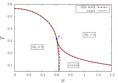
Figure 1: (color online) Phase diagram of the GN model in $1+1$ dimensions in the $(T,\mu)$ plane. The temperature $T$ and the chemical potential $\mu$ are measured in units of the vacuum fermion mass. Our results for the phase boundary between the chirally symmetric phase ($M_{0}=0$) and the phases with spontaneously broken chiral symmetry agree with the exact solution Thies and Urlichs (2003); Schnetz et al. (2004, 2006). The boundary between the phase with a homogeneous chiral condensate ($M_{0}\neq 0,Q=0$) and the crystal phase ($M_{0}\neq 0,Q\neq 0$) is not reproduced correctly within our present study, see main text for details.

In Fig. 1, we show the phase diagram in the $(T,\mu)$ plane. The solid black lines depict the exact solutions for the phase boundaries Schnetz et al. (2004, 2006). Overall, three different phases are found to exist: a chirally symmetric phase ($M_{0}=0$), a phase with spontaneously broken chiral symmetry described by a homogeneous ground state ($M_{0}\neq 0,Q=0$), and an inhomogeneous/crystal phase $(M_{0}\neq 0,Q\neq 0)$. The latter is characterized by a spontaneous breakdown of the chiral symmetry as well as of the translation symmetry. Strictly speaking, there is still a residual discrete translation symmetry as the ground-state is described by a periodic function for all values of $T$ and $\mu$.

It was found in Refs. Thies and Urlichs (2003); Schnetz et al. (2004) that the three phases are separated by second-order phase transitions. The associated phase transition lines meet at a Lifshitz point. Note that both the phase with a homogeneous condensate and the one with an inhomogeneous condensate are characterized by chiral symmetry breaking. The boundary between these two phases is solely associated with translation symmetry breaking where the value of $Q$ of the ground-state configuration acts as an order parameter. We add here that within the phase with a nonvanishing homogeneous condensate, there exists a so-called metastable phase in which the order-parameter potential, apart from an absolute minimum at $\bar{\sigma}\neq 0$, acquires a local minimum at $\bar{\sigma}=0$, see Ref. Wolff (1985). Note also that the originally found first-order transition line – obtained by allowing for homogeneous condensates only – between the phases with finite and vanishing homogeneous condensates Wolff (1985) lies within the crystal phase. In the correct phase diagram Thies and Urlichs (2003); Schnetz et al. (2004) depicted in Fig. 1, however, this line does not describe a phase transition in the ground-state of the theory anymore.

Let us now discuss the results from a minimization of the effective order-parameter potential $V$, see Eq. (17). In perfect agreement with our analytic analysis of the fermion doubling approach in Sects. II.2 and II.3, we find that the boundary between the phases with broken chiral symmetry and the chirally symmetric phase is recovered correctly. The position of the Lifshitz point, denoted by $P_{L}$ in Fig. 1, is reproduced correctly as well, within our numerical errors. Moreover, we would like to emphasize that the dependence of $Q$ on $\mu$ along the transition line between the crystal phase and the chirally symmetric phase is in perfect agreement with the exact result for all studied values of $\mu$. In particular, we find that $Q(\mu)$ tends to zero continuously when the Lifshitz point is approached. For large $\mu\gg M_{0}$, on the other hand, we have $Q(\mu)\sim\mu$, as naively expected from a dimensional analysis.

Our result for the boundary between the phase with a homogeneous condensate and the crystal phase differs from the exact solution Thies and Urlichs (2003); Schnetz et al. (2006). To be more specific, close to the Lifshitz point, we still find that our fermion doubling approach yields the correct result for the transition line. Decreasing the temperature, however, we observe that our result starts to deviate from the exact solution. Remarkably, as can be seen from Fig. 1, it is still well-compatible with the exact phase boundary. In any case, also with our present approach, we obtain that the originally found first-order transition line lies still within the crystal phase.

At this point, we recall that the transition between the phase with a homogeneous condensate and the crystal phase is not related to chiral symmetry breaking. The respective phase boundary only signals translation symmetry breaking as measured by the value of $Q$ of the ground-state configuration. The associated phase transition was found to be of second order in the exact solution of the GN model Thies and Urlichs (2003); Schnetz et al. (2004). With our fermion doubling approach, we instead find a weak first-order transition. The discrepancy between the exact solution and our results in the position and the nature of the transition line can be traced back to the fact that the ground-state of the crystal phase approaches a so-called kink-antikink solution in the zero-temperature limit Brzoska and Thies (2002); Thies (2004); Thies and Urlichs (2003). Thus, higher orders in the Fourier decomposition of the ground state configuration are expected to become increasingly important when the temperature is decreased and our simple single cosine ansatz for $\bar{\sigma}$ does not represent an adequate approximation anymore. Moreover, we emphasize again that our arguments concerning the possibility of a reliable determination of the phase boundaries in Sect. II.3 hold only for second-order chiral phase transitions for which the curvature of the effective potential at $\bar{\sigma}=0$ serves as an order parameter. The latter is not the case for the transition between a crystal phase and a homogeneous phase, where both phases are governed by chiral symmetry breaking. Here, higher $n$-point functions may indeed become relevant. In the present case, in particular for the GN model in $1+1$ dimensions, the importance of higher $n$-point functions is to be expected since the order-parameter potential acquires an additional local – but not global – minimum at $\bar{\sigma}=0$ in the phase with a homogeneous condensate close to the transition to the crystal phase, see also our discussion above.

In contrast to the momentum structure of the first non-trivial expansion coefficient $V^{(2)}$ of the order-parameter potential (see Eq. (26)), the ones for the higher-order coefficients determined from our fermion doubling approach do in general not agree with those from an exact treatment of the fermion determinant. Still, the results for all expansion coefficients from our present approach are identical to the exact ones for $Q=0$. Since the transition line to the crystal phase is of second order in $Q$ Schnetz et al. (2004, 2006) implying that the homogeneous ground state is continuously connected to the inhomogeneous one, it is still reasonable to expect that our fermion doubling approach allows to give a reliable first estimate for the position of the transition line, provided that the exact ground-state can be well described by a simple ansatz of the form (10). For the 1+1 dimensional GN model, this is indeed the case in the vicinity of the chiral phase boundary Schnetz et al. (2004, 2006) and explains why our result for the transition line from the phase with $M_{0}\neq 0$ and $Q=0$ to the crystal phase is still in excellent agreement with the exact solution close to the Lifshitz point. As discussed above, for lower temperatures, our simple ansatz for $\bar{\sigma}$ does no longer provide an adequate description of the ground state and the agreement with the exact solution for the transition line is only qualitative, see Fig. 1. In any case, the overall agreement of our results based on the fermion doubling trick with the exact results is quite impressive for the entire phase diagram, in particular given the simplicity of our fermion doubling approach.

IV Conclusions

In the present work we have introduced and critically discussed a simple “fermion doubling trick” which allows us to search for the emergence of inhomogeneous phases in the phase diagram of fermionic models. Our approach is efficient in the sense that it is based on a straightforward minimization of the effective order-parameter potential (of complexity analogous to standard mean-field studies assuming homogeneous condensates) and does not require any exact diagonalization methods, such as the solution of Bogoliubov-de Gennes-type equations. Exemplarily employing our fermion doubling trick for the $d=$1+1 dimensional GN model, we have indeed found that the chiral phase boundary agrees identically with the exact solution in Refs. Thies and Urlichs (2003); Schnetz et al. (2004, 2006), including the prediction of the emergence of a crystal phase. Moreover, our result for the transition line between the phase with a homogeneous chiral condensate and the crystal phase approaches the exact solution close to the Lifshitz point and agrees at least qualitatively with the exact solution for low temperatures.

In order to show that the chiral phase boundary is indeed predicted correctly by our fermion doubling approach, we have analyzed the two-point function and found that its momentum structure agrees with the one from an exact computation. In addition, we have argued that this is not only the case for the GN model in $1+1$ dimensions but also expected for Nambu-Jona-Lasinio-type models and also applies to these types of models in higher dimensions, as long as only one-dimensional modulations of the ground state are considered. Apart from the chiral phase boundary, we have also pointed out why our fermion doubling approach may still yield a reasonable first estimate for the transition line between the phase with a homogeneous chiral condensate and the crystal phase for a given model. From our discussion, it is also clear that our present approach is not capable of determining the exact ground-state energy, in particular within the crystal phase. By construction, the strength of the approach is rather to detect the emergence of crystal phases in the phase diagram of fermionic theories in a comparatively simple and efficient way and thereby to draw a more detailed picture of the interaction dynamics underlying these theories. In this respect, our fermion doubling approach may help to guide future phase diagram studies and assist as well as direct other more powerful (exact) methods, such as exact diagonalization, in the search for the ground state of fermionic models.

Acknowledgments.–  The authors thank G. V. Dunne, S. Rechenberger and M. Thies for useful discussions and M. Thies also for useful comments on the manuscript. J.B. and D.R. acknowledge support by HIC for FAIR within the LOEWE program of the State of Hesse as well as by the DFG under Grant BR 4005/2-1.

References

- Fulde and Ferrell (1964) P. Fulde and R. A. Ferrell, Phys. Rev. 135, A550 (1964).
- Larkin and Ovchinnikov (1965) A. I. Larkin and Y. N. Ovchinnikov, Sov. Phys. JETP 20, 762 (1965).
- Jackiw and Schrieffer (1981) R. Jackiw and J. Schrieffer, Nucl.Phys. B190, 253 (1981).
- Mertsching and Fischbeck (1981) J. Mertsching and H. J. Fischbeck, phys. stat. sol. (b) 103, 783 (1981).
- Machida and Nakanishi (1984) K. Machida and H. Nakanishi, Phys. Rev. B 30, 122 (1984).
- Chodos et al. (1999) A. Chodos, H. Minakata, and F. Cooper, Phys.Lett. B449, 260 (1999), arXiv:hep-ph/9812305 [hep-ph] .
- Kleinert and Babaev (1998) H. Kleinert and E. Babaev, Phys.Lett. B438, 311 (1998), arXiv:hep-th/9809112 [hep-th] .
- Bulgac and Forbes (2008) A. Bulgac and M. M. Forbes, Phys.Rev.Lett. 101, 215301 (2008), arXiv:0804.3364 [cond-mat.supr-con] .
- (9) J. E. Baarsma and H. T. C. Stoof, arXiv:1212.5450 [cond-mat.quant-gas] .
- Radzihovsky (2012) L. Radzihovsky, Physica C: Superconductivity 481, 189 (2012).
- Roscher et al. (2014) D. Roscher, J. Braun, and J. E. Drut, Phys. Rev. A89, 063609 (2014), arXiv:1311.0179 [cond-mat.quant-gas] .
- Schon and Thies (2000) V. Schon and M. Thies, Phys.Rev. D62, 096002 (2000), arXiv:hep-th/0003195 [hep-th] .
- (13) V. Schon and M. Thies, hep-th/0008175 [hep-th] .
- Schnetz et al. (2004) O. Schnetz, M. Thies, and K. Urlichs, Annals Phys. 314, 425 (2004), arXiv:hep-th/0402014 [hep-th] .
- Schnetz et al. (2006) O. Schnetz, M. Thies, and K. Urlichs, Annals Phys. 321, 2604 (2006), arXiv:hep-th/0511206 [hep-th] .
- Basar and Dunne (2008a) G. Basar and G. V. Dunne, Phys. Rev. Lett. 100, 200404 (2008a), arXiv:0803.1501 [hep-th] .
- Basar and Dunne (2008b) G. Basar and G. V. Dunne, Phys.Rev. D78, 065022 (2008b), arXiv:0806.2659 [hep-th] .
- Basar et al. (2009) G. Basar, G. V. Dunne, and M. Thies, Phys.Rev. D79, 105012 (2009), arXiv:0903.1868 [hep-th] .
- Bringoltz (2007) B. Bringoltz, JHEP 0703, 016 (2007), arXiv:hep-lat/0612010 [hep-lat] .
- Bringoltz (2009) B. Bringoltz, Phys.Rev. D79, 125006 (2009), arXiv:0901.4035 [hep-lat] .
- Nickel (2009) D. Nickel, Phys. Rev. D80, 074025 (2009), arXiv:0906.5295 [hep-ph] .
- Kojo et al. (2010) T. Kojo, Y. Hidaka, L. McLerran, and R. D. Pisarski, Nucl.Phys. A843, 37 (2010), arXiv:0912.3800 [hep-ph] .
- (23) M. Buballa and S. Carignano, arXiv:1406.1367 [hep-ph] .
- Casalbuoni and Nardulli (2004) R. Casalbuoni and G. Nardulli, Rev.Mod.Phys. 76, 263 (2004), arXiv:hep-ph/0305069 [hep-ph] .
- Thies (2006) M. Thies, J.Phys. A39, 12707 (2006), arXiv:hep-th/0601049 [hep-th] .
- Brzoska and Thies (2002) A. Brzoska and M. Thies, Phys.Rev. D65, 125001 (2002), arXiv:hep-th/0112105 [hep-th] .
- Thies (2004) M. Thies, Phys. Rev. D69, 067703 (2004), arXiv:hep-th/0308164 [hep-th] .
- Thies and Urlichs (2003) M. Thies and K. Urlichs, Phys. Rev. D67, 125015 (2003), arXiv:hep-th/0302092 [hep-th] .
- Mermin and Wagner (1966) N. D. Mermin and H. Wagner, Phys. Rev. Lett. 17, 1133 (1966).
- Hohenberg (1967) P. C. Hohenberg, Phys. Rev. 158, 383 (1967).
- Karbstein and Thies (2007) F. Karbstein and M. Thies, Phys. Rev. D75, 025003 (2007), arXiv:hep-th/0610243 [hep-th] .
- de Forcrand and Philipsen (2002) P. de Forcrand and O. Philipsen, Nucl.Phys. B642, 290 (2002), arXiv:hep-lat/0205016 [hep-lat] .
- Lombardo (2006) M. Lombardo, PoS CPOD2006, 003 (2006), arXiv:hep-lat/0612017 [hep-lat] .
- Philipsen (2013) O. Philipsen, Prog.Part.Nucl.Phys. 70, 55 (2013), arXiv:1207.5999 [hep-lat] .
- Ebert et al. (2011) D. Ebert, N. Gubina, K. Klimenko, S. Kurbanov, and V. C. Zhukovsky, Phys. Rev. D84, 025004 (2011), arXiv:1102.4079 [hep-ph] .
- Gubina et al. (2012) N. Gubina, K. Klimenko, S. Kurbanov, and V. C. Zhukovsky, Phys. Rev. D86, 085011 (2012), arXiv:1206.2519 [hep-ph] .
- Ebert et al. (2014) D. Ebert, T. Khunjua, K. Klimenko, and V. C. Zhukovsky, Int. J. Mod. Phys. Rev.Phys. A29, 1450025 (2014), arXiv:1306.4485 [hep-th] .
- Feinberg (2004) J. Feinberg, Annals Phys. 309, 166 (2004), arXiv:hep-th/0305240 [hep-th] .
- Gross and Neveu (1974) D. J. Gross and A. Neveu, Phys.Rev. D10, 3235 (1974).
- Hubbard (1959) J. Hubbard, Phys. Rev. Lett. 3, 77 (1959).
- Stratonovich (1957) R. Stratonovich, Dokl. Akad. Nauk. 115, 1097 (1957).
- Pausch et al. (1991) R. Pausch, M. Thies, and V. Dolman, Z.Phys. A338, 441 (1991).
- Wolff (1985) U. Wolff, Phys.Lett. B157, 303 (1985).
- Nambu and Jona-Lasinio (1961a) Y. Nambu and G. Jona-Lasinio, Phys.Rev. 122, 345 (1961a).
- Nambu and Jona-Lasinio (1961b) Y. Nambu and G. Jona-Lasinio, Phys.Rev. 124, 246 (1961b).