Rayleigh-Bénard Instability in Graphene

Abstract

Motivated by the observation that electrons in graphene, in the hydrodynamic regime of transport, can be treated as a two-dimensional ultra-relativistic gas with very low shear viscosity, we examine the existence of the Rayleigh-Bénard instability in a massless electron-hole plasma. Firstly, we perform a linear stability analysis, derive the leading contributions to the relativistic Rayleigh number, and calculate the critical value above which the instability develops. By replacing typical values for graphene, such as thermal conductivity, shear viscosity, temperature, and sample sizes, we find that the instability might be experimentally observed in the near future. Additionally, we have performed simulations for vanishing reduced chemical potential and compare the measured critical Rayleigh number with the theoretical prediction, finding good agreement.

I Introduction

Graphene, consisting of literally a single carbon monolayer, represents the first instance ever of a truly two-dimensional material. Due to the special symmetries of the honeycomb lattice, electrons in graphene are shown to behave like an effective Dirac fluid of massless, chiral quasi-particles, propagating at a Fermi speed of about $v_{F}\approx 1.1\times 10^{6}$m/s, cf. Refs. Novoselov et al. (2004, 2005). Recent theoretical insights Müller and Sachdev (2008); Müller et al. (2008); Fritz et al. (2008); Müller et al. (2009) have opened up the possibility to describe the electrical current on graphene close to the Dirac point as a classical relativistic fluid when inelastic electron-electron and electron-hole scattering dominate over elastic electron-impurity and electron-phonon processes. Since electrons are about $300$ times slower than photons, their mutual interaction is proportionately enhanced, leading to an effective fine-structure constant $\alpha_{gr}=e^{2}/\hbar v_{F}\sim 1$. As a result of such strong interactions, it has been recently proposed that this peculiar 2D graphene electron gas should be characterised by an exceptionally low viscosity/entropy ratio (near-perfect fluid), coming close to the famous AdS-CFT lower bound Kovtun et al. (2005) conjectured for quantum-chromodynamic fluids, such as quark-gluon plasmas. This spawns the exciting prospect of observing electronic pre-turbulence in graphene samples, as first pointed out in Ref. Müller et al. (2009) and confirmed by recent numerical simulations Mendoza et al. (2011).
One of the most common hydrodynamic instabilities, is the Rayleigh-Bénard, which has been studied experimentally since 1901 Bénard (1901), and first described theoretically by Lord Rayleigh in 1916 Rayleigh (1916). Here, one observes the creation of convection cells, which couple the heat and particle flow, where the driving mechanisms are the temperature gradient and the buoyancy force (typically caused by gravity Chandrasekhar (1961)). This instability appears in many scientific and industrial applications Massaioli et al. (1993); Ahlers et al. (2012); Moon and Chung (2014), and is still subject of current research.
Since electrons and holes in graphene can be described by relativistic hydrodynamics, it opens the question whether the Rayleigh-Bénard instability can be also observed. Although gravity in this case is negligible, we can use an external electric field to mimic its effects. In the classical case, the Rayleigh-Bénard instability will always appear if the Rayleigh number Chandrasekhar (1961), defined by

$$\mathrm{Ra}_{\text{cl}}=\frac{\alpha g\beta\rho c_{V}l^{4}}{\kappa\eta}\text{ ,}$$ (1)

exceeds a critical value. Here, $\alpha$ is the thermal volume expansion coefficient, $g$ the gravitational acceleration, $\beta$ the uniform adverse temperature gradient, $c_{V}$ the specific heat at constant volume, $\rho$ the mass density, $l$ the length of the system parallel to the gravitational force, $\kappa$ the thermal conductivity, and $\eta$ the shear viscosity. From this expression, we can notice that for low values of shear viscosity and thermal conductivity, we obtain a large Rayleigh number, and consequently, they contribute to the appearance of the instability. Graphene’s electronic fluid has a very low shear viscosity but a high thermal conductivity Balandin et al. (2008), therefore, it is not straightforward to judge the existence of the instability, under actual experimental conditions. In order to answer this question, we first introduce a linear stability analysis in the context of relativistic hydrodynamics, which has not been formulated before, to the best of our knowledge, and calculate the critical relativistic Rayleigh number. We also perform numerical simulations of electronic flow in graphene in order to observe the convection rolls, and to validate our linear stability analysis. By studying the parameter regime, in which the instability can be observed in graphene, we have found that under actual experimental conditions, it is unlikely to observe the instability, but since the construction of larger samples of graphene is a target in current research, it might be observed in the near future.
This work is organised as follows. In Section II we write the macroscopic equations from the relativistic Boltzmann transport theory for graphene in the “hydrodynamic regime” Fritz et al. (2008). These partial differential equations build the basis for the linear stability analysis, which will be derived in Section III. Thereby, we define the dimensionless relativistic Rayleigh number, determine its critical value, which marks the onset of the instability, and investigate the experimental realizability of the phenomenon. The Einstein summation convention and the signature $(+,-,-)$ for the Minkowski metric $g^{\alpha\beta}$ are used. Greek indices run from 0 to 2 whereas Latin indices can only take the values 1 and 2. The other constants which are used throughout the article are $k_{B}$ for the Boltzmann constant, $\hbar\equiv h/2\pi$ for the reduced Planck constant, and $e$ for the absolute value of the elementary electric charge. In Section IV, we perform simulations of the electron flow for vanishing reduced chemical potential. For this purpose, we first extend the relativistic lattice Boltzmann developed in Ref. Öttinger et al. (2013), analyse the functional form of the shear viscosity and thermal conductivity, and validate our implementation of the external force. Finally, the critical relativistic Rayleigh number is measured and compared to the theoretical prediction. As a general introduction to the lattice Boltzmann method and its extension to relativistic dynamics and quantum statistics we refer the reader to Refs. Benzi et al. (1992), Mendoza et al. (2010) and Uehling and Uhlenbeck (1933).

II Hydrodynamic regime overview

In the hydrodynamic regime Müller et al. (2009); Fritz et al. (2008), it is known that carriers in graphene behave as a two-dimensional relativistic fermionic plasma whose quasi-particles are charged, nearly massless, and moving at the Fermi speed $c\equiv v_{F}$. Henceforth, we will denote the Fermi speed by $c$. In order to describe the collision-dominated electron-transport in this material, we use the relativistic Boltzmann equation Müller et al. (2009)

$$p^{\alpha}\frac{\partial f_{\sigma}}{\partial x^{\alpha}}+\sigma K^{\alpha}\frac{\partial f_{\sigma}}{\partial p^{\alpha}}=\mathcal{J}^{(\sigma)}_{\text{coll}}\text{ ,}$$ (2)

with $\sigma=\mp$ denoting electrons ($+$) and holes ($-$), $p^{\alpha}$ being the (pseudo) 3-momentum and $\sigma K^{\alpha}=\sigma F^{\alpha\beta}p_{\beta}$ being the electromagnetic 3-force acting on the electron/hole fluid component with distribution function $f_{\sigma}$ in phase-space $\left(\vec{x},\vec{p}\right)$ at time $t$ Cercignani and Kremer (2002). Here, $J^{(\sigma)}_{\text{coll}}$ denotes the collision operator, further explained in Ref. Fritz et al. (2008). $F^{\alpha\beta}$ is the “electromagnetic field strength tensor”, defined as

$$F^{\alpha\beta}=\begin{pmatrix}0&eE_{1}/c&eE_{2}/c\\ -eE_{1}/c&0&eB\\ -eE_{2}/c&-eB&0\end{pmatrix}\text{ ,}$$

with $\vec{E}=(E_{1},E_{2},0)$ and $\vec{B}=(0,0,B)$ being the electric and magnetic fields, respectively. This formulation implies that the Coulomb interactions are invariant under Lorentz transformations defined with the speed of Fermi. Obviously, in fact they spread at the real speed of light, $c_{L}\gg c$, and therefore, they break the Lorentz invariance of our system. However, since we will deal with fluid flows at low speeds we can work in the laboratory frame, cf. Ref. Müller et al. (2009). The contravariant “charge flow” $J^{\alpha}$ and energy-momentum tensor $T^{\alpha\beta}$ are defined as first and second moment of the distribution function:

$$J^{\alpha}(\vec{x},t) \equiv\langle p_{\sigma}^{\alpha}\rangle_{\sigma}\equiv\sum_{\sigma}c\int\!\frac{\mathrm{d}\vec{p}}{p_{0}}\hskip 4.30554ptp_{\sigma}^{\alpha}f_{\sigma}(t,\vec{x},\vec{p})\text{ ,}$$ (3)

$$T^{\alpha\beta} \equiv\langle p_{\sigma}^{\alpha}p_{\sigma}^{\beta}\rangle_{\sigma}\equiv\sum_{\sigma}c\int\!\frac{\mathrm{d}\vec{p}}{p_{0}}\hskip 4.30554ptp_{\sigma}^{\alpha}p_{\sigma}^{\beta}f_{\sigma}(t,\vec{x},\vec{p})\text{ ,}$$ (4)

with $p_{\sigma}^{\alpha}=\sigma p^{\alpha}$. Using Eq. (2), the definitions (3), (4), and integrating by parts, the macroscopic conservation equations for charge, energy and momentum can be obtained,

$$\partial_{\alpha}J^{\alpha} =0\text{ ,}$$ (5)

$$\partial_{\beta}T^{\alpha\beta} =F^{\alpha\nu}J_{\nu}\text{ .}$$ (6)

Following an idea expressed in Ref. Landau and Lifshitz (1987), we employ the Eckart decomposition, cf. Ref. Cercignani and Kremer (2002), with respect to the 3-velocity $U^{\alpha}\equiv\frac{\left(c,u_{1},u_{2}\right)^{\alpha}}{\sqrt{1-|\vec{u}|^{2}/c^{2}}}$ of the “charge flow” $J^{\alpha}$, cf. Ref. Wangsness (1986), i.e. the current 3-vector and the energy-momentum tensor for the case of the viscous heat conducting fluid are given by

$$J^{\alpha}=\hskip 2.15277pt nU^{\alpha}\text{ ,}$$ (7)

$$T^{\alpha\beta}=\hskip 2.15277pt \epsilon\frac{U^{\alpha}U^{\beta}}{c^{2}}-\left(p+\omega\right)\Delta^{\alpha\beta}+p^{<\alpha\beta>}$$

$$+\frac{1}{c^{2}}\left(U^{\alpha}q^{\beta}+U^{\beta}q^{\alpha}\right)\text{,}$$ (8)

where $n(\vec{x},t)$ is the charge density divided by $e$, $\epsilon$ the internal energy density, $p$ the hydrostatic pressure, $\omega$ the dynamic pressure, $q^{\alpha}$ the contravariant heat flux and $p^{<\alpha\beta>}$ the pressure deviator in local equilibrium. Assuming that linear irreversible thermodynamics can be applied and using the procedure outlined in Ref. Cercignani and Kremer (2002), we find for the constitutive equations

$$p^{<\alpha\beta>} =2\eta\left[\frac{1}{2}\left(\Delta^{\alpha}_{\gamma}\Delta^{\beta}_{\delta}+\Delta^{\alpha}_{\delta}\Delta^{\beta}_{\gamma}\right)-\frac{1}{3}\Delta^{\alpha\beta}\Delta_{\gamma\delta}\right]\nabla^{\gamma}U^{\delta}\text{ ,}$$

$$q^{\alpha} =\kappa\left(\nabla^{\alpha}T-\frac{T}{c^{2}}DU^{\alpha}\right)\text{ ,}$$ (9)

$$\omega =-\nu\nabla_{\alpha}U^{\alpha}\text{ ,}$$

where $\eta$ and $\nu$ stand for the shear and bulk viscosities, and $\kappa$ for the thermal conductivity. $\Delta^{\alpha\beta}\equiv g^{\alpha\beta}-\frac{U^{\alpha}U^{\beta}}{c^{2}}$ stands for the projector into the space perpendicular to $U^{\alpha}$, $D\equiv U^{\alpha}\partial_{\alpha}$ for the convective time-derivative, and $\nabla^{\alpha}\equiv\Delta^{\alpha\beta}\partial_{\beta}$ for the gradient operator in this decomposition. It should be noted that the direct contribution of the electromagnetic fields to the heat flux vanishes due to the antisymmetry of the field strength tensor. However, they have an indirect contribution through the term $DU^{\alpha}$.

II.1 Non-relativistic current flow

Assuming $|\vec{u}|/c\ll 1$, we simplify the conservation equations (5) and (6) to

$$0 =\partial_{t}n+\vec{\nabla}\cdot\left(n\vec{u}\right)\text{ ,}$$ (10)

$$\varphi =\partial_{t}\epsilon+\vec{\nabla}\cdot\left[(\epsilon+p)\vec{u}\right]+\vec{\nabla}\cdot\vec{q}+n\vec{u}\cdot e\vec{E}\text{ ,}$$ (11)

$$\vec{\psi} =\frac{\partial_{t}}{c^{2}}\left[\left(\epsilon+p\right)\vec{u}+\vec{q}\right]+\vec{\nabla}p+ne\vec{E}\text{ ,}$$ (12)

with $\varphi\equiv\partial_{i}\left[\left(\nu-\frac{2\eta}{3}\right)u_{i}\left(\vec{\nabla}\cdot\vec{u}\right)+\eta\vec{u}\cdot\left(\vec{\nabla}u_{i}+\partial_{i}\vec{u}\right)\right]$ being the change in energy due to dissipation and $\psi_{i}\equiv-\partial_{i}\left[\left(\frac{2\eta}{3}-\nu\right)\vec{\nabla}\cdot\vec{u}\right]+\partial_{j}\left[\eta\left(\partial_{i}u_{j}+\partial_{j}u_{i}\right)\right]$ the viscous term. To get those equations we have used the approximations from Ref. Cercignani and Kremer (2002) for the expressions (7) and (8), and recovered the Fourier law of heat conduction $\vec{q}=-\kappa\vec{\nabla}T$.

III Linear Stability Analysis

In analogy to the classical Rayleigh-Bénard problem Severin and Herwig (2001), we study a system with constant volume, confined to $(x_{1},x_{2})\in\mathbb{R}\times[-l/2,l/2]$ with $l$ being the length of our system. It has two thermal contacts at $x_{2}=\pm l/2$ with temperatures $T_{\pm}$, respectively, and feels a constant homogeneous external electric field $\vec{E}_{\text{ext}}=E_{\text{ext}}\hat{e}_{2}$. We consider our system thermally isolated elsewhere, which can be achieved, for example, by a freely suspended sheet Seol et al. (2010), or using supports with a much smaller thermal conductivity. However, the contact with another material may require to consider a graphene-substrate interaction which can alter the dynamics. For the description of the electron-hole fluid we choose the velocity $\vec{u}$, the temperature $T$, the volume $V$ and the electro-chemical potential $\mu$ as state variables. Following the procedure outlined in Ref. Chandrasekhar (1961) we make a linear stability analysis by perturbing the stationary, non-homogeneous, quiescent state characterized by ($\vec{u}=0$, $T=\bar{T}$, $\mu=\bar{\mu}$). This state is chosen to simplify the theoretical analysis. By symmetry, the variables $\bar{T}$ and $\bar{\mu}$ only depend on $x_{2}/l$. They can be calculated by solving the ordinary differential equations

$$\bar{T}^{\prime}\kappa^{\prime}(\bar{T},\bar{\mu})+\bar{T}^{\prime\prime}\kappa(\bar{T},\bar{\mu}) =0\text{ ,}$$ (13)

$$p^{\prime}(\bar{T},\bar{\mu})-lE_{2}(\bar{T},\bar{\mu})en(\bar{T},\bar{\mu}) =0\text{ ,}$$ (14)

which follow from Eqs. (11) and (12) under the stated assumptions. It should be noted that the average electric field $\bar{E}_{2}=E_{2}(\bar{T},\bar{\mu})$ not only contains external information, as the fluid components also experience an internal electric field due to intrinsic distributions of charge.

III.1 Perturbation equations

Writing for each fluid quantity in Eqs. (10) to (12), $X=\bar{X}+\tilde{X}$ with $X\in\{T,\epsilon,p,n,u_{i},E_{i},\kappa,\eta,\nu\}$ and ignoring non-linear terms in the perturbations $\tilde{X}$ we find for the perturbation equations

$$\partial_{t}\tilde{n}+\bar{n}^{\prime}u_{2}+\bar{n}\partial_{i}\tilde{u}_{i} =0\text{ ,}$$ (15)

$$\partial_{t}\tilde{\epsilon}+\bar{\epsilon}^{\prime}\tilde{u}_{2}+c^{2}\bar{\rho}\partial_{i}\tilde{u}_{i}+\partial_{i}\tilde{q}_{i} =0\text{ ,}$$ (16)

$$\bar{\rho}\partial_{t}\tilde{u}_{i}+\frac{\partial_{t}\tilde{q}_{i}}{c^{2}}-\partial_{j}\left[\bar{\eta}\left(\partial_{i}\tilde{u}_{j}+\partial_{j}\tilde{u}_{i}\right)\right]+\partial_{i}\tilde{p}+\tilde{f}_{i} =$$

$$\partial_{i}\left[\left(\frac{2\bar{\eta}}{3}-\bar{\nu}\right)\partial_{j}\tilde{u}_{j}\right]$$ , (17)

where we have defined $\bar{\rho}\equiv\frac{\bar{\epsilon}+\bar{p}}{c^{2}}$ as mass density,

$$\tilde{q}_{i} \equiv\bar{\kappa}\partial_{i}\tilde{T}+\tilde{\kappa}\bar{T}^{\prime}\delta_{i2}\text{ , and}$$

$$\tilde{f}_{i} \equiv\tilde{n}e\bar{E}_{2}\delta_{i2}+\bar{n}e\tilde{E}_{i}\text{ ,}$$

for the perturbations of the heat flux and force density, respectively. In addition, we assume that the thermodynamics of the plasma is very similar to a photon gas. Hence, we know that its internal energy is mainly determined by the state variables of temperature $T$ and volume $V$, i.e. $\tilde{\epsilon}\approx\bar{c}_{V}\tilde{T}$ with $c_{V}$ being the volume-specific heat capacity at constant volume. Employing the Oberbeck-Boussinesq approximation Chandrasekhar (1961), for which the electric field takes the role of the gravitational field, the perturbation equations in linear approximation become

$$\partial_{i}\tilde{u}_{i}=\hskip 2.15277pt 0\text{ ,}$$ (18)

$$\partial_{t}\tilde{T}=\hskip 2.15277pt -\beta_{R}\tilde{u}_{2}+\frac{\kappa_{R}}{\left(c_{V}\right)_{R}}\Delta\tilde{T}\text{ ,}$$ (19)

$$\partial_{t}\tilde{u}_{i}=\hskip 2.15277pt -\left(\alpha_{q}\right)_{R}a_{R}\tilde{T}\delta_{i2}-\frac{n_{R}}{\rho_{R}}e\tilde{E}_{i}+\frac{\eta_{R}}{\rho_{R}}\Delta\tilde{u}_{i}$$

$$-\frac{1}{\rho_{R}}\partial_{i}\left(\tilde{p}-\frac{\kappa_{R}}{c^{2}}\partial_{t}\tilde{T}\right)\text{ ,}$$ (20)

with reference temperature $T_{R}=\bar{T}(x_{2}=0)$, gradient $\beta_{R}\equiv\bar{T}^{\prime}(x_{2}=0)$, reference electro-chemical potential $\mu_{R}=\bar{\mu}(x_{2}=0)$, reference acceleration $a_{R}\equiv\frac{n_{R}eE_{R}}{\rho_{R}}$, electric field $E_{R}\equiv\bar{E}_{2}(T_{R},\mu_{R})$ and reference thermal charge expansion coefficient $\left(\alpha_{q}\right)_{R}\equiv\frac{1}{n_{R}}\left.\frac{\partial n}{\partial T}\right|_{T=T_{R},\mu=\mu_{R}}$. The approximation will be reasonable if variations in these properties primarily stem from temperature fluctuations and $\frac{T_{+}-T_{-}}{T_{+}+T_{-}}\ll 1$ holds. Higher order terms, which include non-Boussinesq effects, can also be considered by the method described in Ref. Herwig and Schäfer (1992). In analogy to Ref. Chandrasekhar (1961), we apply the curl operator twice on Eq. (20) to get rid of the gradients and use the component parallel to the applied electric field

$$\left(\frac{\eta_{R}}{\rho_{R}}\Delta-\partial_{t}\right)\left[\Delta\tilde{u}_{2}-\partial_{2}\partial_{i}\tilde{u}_{i}\right]=\left(\alpha_{q}\right)_{R}a_{R}\partial_{1}^{2}\tilde{T}-\frac{n_{R}}{\rho_{R}}e\partial_{t}\partial_{1}\tilde{B}\text{.}$$

From the Maxwell-Ampère equation Jackson (1999), we can deduce

$$\partial_{t}\partial_{1}\tilde{B}\approx-\mu_{0}en_{R}\partial_{t}\tilde{u}_{2}-\mu_{0}\epsilon_{0}\partial_{t}^{2}\tilde{E}_{2}\text{ ,}$$

with $\mu_{0}$ and $\epsilon_{0}$ being the vacuum permeability and permittivity, respectively. In this form, we realize that the contribution of this term to the overall dynamics is negligible, since $\frac{\mu_{0}e^{2}n^{2}_{R}}{\rho_{R}}\ll 1$ and $\frac{\mu_{0}\epsilon_{0}en_{R}}{\rho_{R}}\ll 1$. Consequently, the final and smaller set of simplified linear perturbation equations reads

$$\partial_{i}\tilde{u}_{i} =0\text{ ,}$$ (21)

$$\partial_{t}\tilde{T} =\beta_{R}\tilde{u}_{2}+\frac{\kappa_{R}}{\left(c_{V}\right)_{R}}\Delta\tilde{T}\text{ ,}$$ (22)

$$\left(\alpha_{q}\right)_{R}a_{R}\partial_{1}^{2}\tilde{T} =\left(\frac{\eta_{R}}{\rho_{R}}\Delta-\partial_{t}\right)\Delta\tilde{u}_{2}\text{ ,}$$ (23)

and has the same form as in Ref. Chandrasekhar (1961). Therefore, we define the Prandtl and relativistic Rayleigh number of this system as

$$\mathrm{Pr} \equiv\frac{\eta_{R}\left(c_{V}\right)_{R}}{\rho_{R}\kappa_{R}}\text{ ,}$$ (24)

$$\mathrm{Ra}_{\text{rel}} \equiv\frac{\left(\alpha_{q}\right)_{R}a_{R}\beta_{R}l^{4}}{\frac{\kappa_{R}}{\left(c_{V}\right)_{R}}\frac{\eta_{R}}{\rho_{R}}}=\frac{\left(\alpha_{q}c_{V}\right)_{R}n_{R}eE_{R}\beta_{R}l^{4}}{\kappa_{R}\eta_{R}}\text{ ,}$$ (25)

by following the method of Ref. Severin and Herwig (2001). In analogy with the classical case, we expect a positive Rayleigh number. Therefore, we find that the possibility for the occurrence of the instability depends on the sign of the product of the temperature gradient, the external electric field and the thermal charge expansion coefficient, as all other parameters are non-negative.

III.2 Analysis into normal modes

Since the equations in the previous subsection have the same form as in the classical case, except for different coefficients, we can draw on the work in Ref. Chandrasekhar (1961) concerning the analysis into normal modes and the calculation of the critical Rayleigh number. Due to the geometry of the problem we can expand any perturbation into the complete set of plane waves and hence write

$$\tilde{T}(x_{1},x_{2},t) =\int\limits_{\mathbb{R}}\!\mathrm{d}k\hskip 4.30554pt\theta_{k}(x_{2})e^{s_{k}t+\imath kx_{1}}\text{ ,}$$ (26)

$$\tilde{u}_{i}(x_{1},x_{2},t) =\int\limits_{\mathbb{R}}\!\mathrm{d}k\hskip 4.30554ptu_{k,i}(x_{2})e^{s_{k}t+\imath kx_{1}}\text{ ,}$$ (27)

with $s_{k}\in\mathbb{C}$. One can show that the imaginary part of $s_{k}$ needs to vanish if one demands non-conducting or transversal-conducting boundaries at $x_{2}=\pm l/2$. These conditions imply for the charge velocity perturbations under consideration of $\partial_{i}\tilde{u}_{i}=0$ that

$$u_{k,1}(x_{2}=\pm l/2) =0\text{ ,}$$ (28)

$$\partial_{2}u_{k,2}(x_{2}=\pm l/2) =0\text{ ,}$$ (29)

for the case of non-conducting, and

$$\partial_{2}u_{k,1}(x_{2}=\pm l/2) =0\text{ ,}$$ (30)

$$\partial_{2}^{2}u_{k,2}(x_{2}=\pm l/2) =0\text{ ,}$$ (31)

for the case of transversal-conducting boundaries on top of $u_{k,2}(x_{2}=\pm l/2)=0$, for both conditions. For the temperature perturbation one needs to require $\theta_{k}(x_{2}=\pm l/2)=0$, since the system is in contact with two heat baths, i.e. its temperature is fixed at the boundaries. We can conclude that the transition from a stable to an unstable situation for our set of equations occurs exactly at $s_{k}=0$. As a result, the critical relativistic Rayleigh number and wave number for non-conducting boundaries at $x_{2}=\pm l/2$ are approximately given by

$$\mathrm{Ra}_{c} \approx 1707.762\text{ ,}$$ (32)

$$k_{c} \approx\frac{3.117}{l}\text{ ,}$$ (33)

which coincides with the classical value Chandrasekhar (1961). The reason for this is the assumption of a non-relativistic current flow, which will lead in linear stability analysis to similar equations as in the classical case, cf. Refs. Chandrasekhar (1961); Severin and Herwig (2001), if the role of mass and charge are interchanged. Therefore, one should find the same critical Rayleigh number. The ultra-relativistic nature of the quasi-particle and the Fermi-Dirac statistics become apparent in the formulae for the constituents of the relativistic Rayleigh number, such as thermal charge expansion coefficient, charge density, thermal conductivity, etc. For transversal-conducting boundaries, the critical Rayleigh number and wave number are given by

$$\mathrm{Ra}_{c} =\frac{27\pi^{4}}{4}\approx 657.51\text{ ,}$$ (34)

$$k_{c} =\frac{\pi}{\sqrt{2}l}\approx\frac{2.221}{l}\text{ .}$$ (35)

Having derived the relativistic Rayleigh number, and its critical value for the onset of the instability, we will now replace the physical values for graphene and see if under actual experimental conditions, it is possible to observe the instability.

III.3 Application to Graphene

Despite its high thermal conductivity, $\kappa_{R}/d\sim 10^{22}\text{ eV/(K\;m\;s)}$, cf. Ref. Lee et al. (2011), with $d\sim 10^{-10}\text{ m}$ being the nominal thickness of graphene, its electronic fluid also has a very low shear viscosity Müller et al. (2009),

$$\eta_{R}\approx C_{\eta}\hbar\left(\frac{k_{B}T_{R}}{\alpha\hbar c}\right)^{2}\{1+\mathcal{O}\left[\log^{-1}(\alpha)\right]\}\sim 10^{-3}\text{ eV s/m}^{2}\text{,}$$

where $C_{\eta}\approx 0.449$ is a constant, $\alpha\equiv e^{2}/\left(\hbar c\varepsilon_{r}\right)\simeq 2.2/\varepsilon_{r}$ is the fine structure constant and $\varepsilon_{r}$ is the relative permittivity. Using Eq. (12) in Ref. Sheehy and Schmalian (2007) we find for the heat capacity at constant volume $\left(c_{V}\right)_{R}\sim 10^{10}\text{ eV}/\left(\text{K m}^{2}\right)$. In the hydrodynamic regime of transport, we deal with a “Dirac liquid”, i.e. we require $n_{R}\sim 10^{13}\text{ m}^{-2}$, cf. Ref. Sheehy and Schmalian (2007). Therefore, to induce that charge density in the graphene sample, we apply an electric field given by $eE_{R}l\sim 10^{-1}\text{ eV}$, such that the Fermi level changes accordingly. In addition, we approximate $\left(\alpha_{q}\right)_{R}\beta_{R}l\approx\frac{T_{+}-T_{-}}{T_{R}}\sim 10^{-2}$. Thus, we can make a crude estimate for the relativistic Rayleigh number of graphene with a length $l\sim 100\mu\text{m}$ and $\varepsilon_{r}\approx 1$ at $T_{R}\approx 100\text{ K}$ to find

$$\mathrm{Ra}_{\text{rel}}^{(gr)}\sim 10^{3}\text{ .}$$ (36)

This magnitude is comparable to the critical Rayleigh number calculated in the previous paragraph. It tells us that the experimental realization is challenging due to the length of about $100\mu\text{m}$ but probably achievable in the near future, since single-layer samples with sizes larger than $70\mu\text{m}$ have already been produced Sun et al. (2010); Balan et al. (2010).

We want to point out that for higher temperatures smaller sample sizes could be used, since the ratio $\left(c_{V}\right)_{R}/\kappa_{R}\sim\mathcal{O}(T^{2})$ and $eE_{R}l\sim\mathcal{O}(T)$ while the remaining parameter combination in the relativistic Rayleigh number is almost unaffected. However electron-phonon interactions will become more pronounced and hence the dynamics could be altered, cf. Refs. Mendoza M. et al. (2013); Bao et al. (2009).

IV Relativistic lattice Boltzmann simulation

In order to test our theoretical predictions we use the method described in Ref. Öttinger et al. (2013) to perform a relativistic lattice Boltzmann simulation of the electrons in graphene for vanishing reduced chemical potential. The collision operator for the particles in Eq. (2) is approximated by an Anderson-Witting collision operator Anderson and Witting (1974), i.e. the relativistic Boltzmann equation is modified to

$$p^{\alpha}\frac{\partial f}{\partial x^{\alpha}}+K^{\alpha}\frac{\partial f}{\partial p^{\alpha}}=-\frac{p_{\alpha}U_{L}^{\alpha}}{c^{2}\tau}\left[f-f_{eq}\right]\text{ ,}$$ (37)

with $\tau$ the relaxation time and $U_{L}^{\alpha}$ being the 3-velocity of the fluid element in Landau-Lifshitz decomposition, i.e. the 3-velocity of the energy-flow, as opposed to our theoretical treatment where we measured with respect to the charge-flow. For the equilibrium distribution we use the ultra-relativistic Fermi-Dirac distribution

$$f_{eq}=\frac{4/h^{2}}{e^{\frac{U_{L}^{\alpha}p_{\alpha}}{k_{B}T}}+1}\text{ ,}$$

which leads to

$$n_{eq} =U_{L}^{\alpha}\langle p_{\alpha}\rangle_{eq}=\frac{\pi}{12}\left(\frac{k_{B}T}{\hbar c}\right)^{2}\text{ ,}$$ (38)

$$\epsilon_{eq} =U_{L}^{\alpha}\langle p_{\alpha}p_{\beta}\rangle_{eq}U_{L}^{\beta}=2p_{eq}\text{ ,}$$ (39)

$$p_{eq} =\frac{3\zeta(3)k_{B}T}{4\pi}\left(\frac{k_{B}T}{\hbar c}\right)^{2}\text{ .}$$ (40)

Then, we perform an expansion into orthogonal polynomials, which are written in appendix A of Ref. Öttinger et al. (2013),

$$f_{eq}(t,\vec{x},p,\vec{v})=\frac{\pi^{2}}{e^{\frac{p}{T_{0}}}+1}\sum_{n,k=0}^{\infty}a_{\underline{i}}^{(nk)}(t,\vec{x})P_{\underline{i}}^{(n)}\left(\vec{v}\right)F^{(k)}\left(p\right),$$

with $\hbar=k_{B}=c=e=1$ and $\vec{p}=p\vec{v}=p(\cos\phi,\sin\phi)$ in polar coordinates. $T_{0}$ is a constant, dimensionless lattice temperature. The relevant coefficients up to $a_{\underline{i}}^{(22)}$ are calculated in Ref. Öttinger et al. (2013). To simplify the computation even further the angle $\phi$ and radius $p$ are discretized such that a numerical quadrature of the expansion exactly reproduces the zeroth, first and second moment of the equilibrium distribution. The corresponding weights and discrete values for the radii can be found in appendix C of Ref. Öttinger et al. (2013). For the angular quadrature, one finds the weights $\alpha^{(\phi)}_{i}=1/6$ and angles $\phi_{i}=\pi/2+(i-1)\pi/3$ with $i\in\{1,2,3,4,5,6\}$, leaving us with a hexagonal unit cell for each radius, see Fig. 1. The obtained lattice site distribution function now evolves in time steps $\delta t=\delta x/c$ according to the lattice Boltzmann algorithm with

$$f_{\vec{q}}(t+\delta t,\vec{x}+\hat{e}_{\vec{q}}\delta t)-f_{\vec{q}}(t,\vec{x}) =$$

$$- \frac{p^{\alpha}U_{\alpha}}{p^{0}\tau}\left[f_{\vec{q}}(t,\vec{x})-f_{\vec{q}}^{(eq)}(t,\vec{x})\right]$$

where $\vec{q}\equiv(q^{\prime},q^{\prime\prime})$ labels the discrete momenta (radius, angle) and $\hat{e}_{\vec{q}}\equiv\vec{v}_{q^{\prime\prime}}=\vec{p}_{\vec{q}}/p_{0}$.

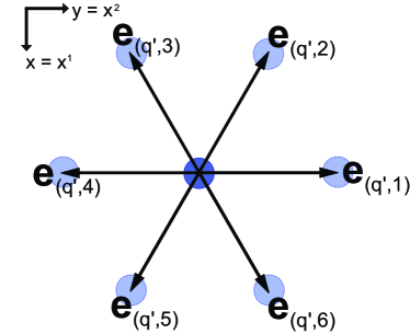
Figure 1: Hexagonal lattice structure according to Ref. Öttinger et al. (2013)

IV.1 External Force Implementation

For including the external force in the simulation, we use the same polynomials as in the expansion of the equilibrium distribution to write

$$mK^{\alpha}\frac{\partial f}{\partial p^{\alpha}}=\frac{1}{e^{\frac{p}{T_{0}}}+1}\sum_{n,k=0}^{\infty}b_{\underline{i}}^{(nk)}P_{\underline{i}}^{(n)}(\vec{v})F^{(k)}(p)\text{ .}$$

In addition, Eqs. (5) and (6) need to be fulfilled, i.e.

$$\int\!\frac{\mathrm{d}\vec{p}}{p^{0}}\hskip 4.30554ptp^{\beta}mK^{\alpha}\frac{\partial f}{\partial p^{\alpha}} =-F^{\beta\nu}N_{\nu}\text{ ,}$$

$$\int\!\frac{\mathrm{d}\vec{p}}{p^{0}}\hskip 4.30554ptmK^{\alpha}\frac{\partial f}{\partial p^{\alpha}} =0\text{ .}$$

From this we infer

$$-F^{0\nu}N_{\nu} =T_{0}^{2}\left[\Gamma_{F}^{(1)}b^{(01)}+c_{10}\Gamma_{F}^{(0)}b^{(00)}\right]\text{ ,}$$

$$-F^{i\nu}N_{\nu} =\frac{T_{0}^{2}}{2}\left[\Gamma_{F}^{(1)}b_{i}^{(11)}+c_{10}\Gamma_{F}^{(0)}b_{i}^{(10)}\right]\text{ ,}$$

$$0 =T_{0}\Gamma_{F}^{(0)}b^{(00)}\text{ ,}$$

and finally choose

$$b^{(01)} =\frac{<p^{i}>E_{i}}{\Gamma_{F}^{(1)}T_{0}^{2}}\text{ ,}$$ (41)

$$b_{i}^{(10)} =\frac{2<p^{0}>E_{i}}{T^{2}_{0}c_{10}\Gamma_{F}^{(0)}}\text{ ,}$$ (42)

with all other coefficients equal to zero. For the validation we measure the velocities $u_{i}\equiv\frac{\langle p^{i}\rangle}{\langle p^{0}\rangle}$ of the particle 3-flow as function of time for very small fields, such that according to Eq. (12) a linear relation between time and velocity is expected. Choosing a homogeneous temperature $T=T_{0}$, constant electric field in $x$-direction and zero energy flux as initial conditions, the result for the first particle-velocity component as shown in Fig. 2 confirms the linear dependence. The fit has been done with the function

$$u_{1}(t)=-\frac{nE_{1}}{\epsilon+p}t+b\text{ ,}$$ (43)

where $b$ is a fit parameter. The fit parameter is not zero, since we impose a vanishing energy flux but measure the charge-velocity. These velocities differ since the electric field creates a heat flux, e.g. Joule heating. We also find that the force does not have any influence on the second velocity component, the density or the pressure, i.e. the absolute value of their temporal change always stays below the numerical error of $10^{-16}$.

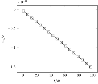
Figure 2: First particle-velocity component $u_{1}$ as a function of time for $E_{1}=10^{-7}$, $E_{2}=0$, $T_{0}=2$, $\tau=\delta t$, system size of $64\times 64$, and periodic boundaries. The solid line represents the fit: $\frac{u_{1}(t)}{c}=\left(\frac{10\pi^{2}}{54\zeta(3)}\frac{t}{\delta t}-2.69\right)\times 10^{-8}$.

IV.2 Shear Viscosity Measurement

In order to measure the shear viscosity we use a Poiseuille flow test. For this purpose, we examine the steady ($t\geq 10^{5}\delta t$) velocity profile obtained by imposing simple bounce-back boundary conditions in $y$-direction, periodic boundaries in $x$-direction, and applying a small, constant, homogeneous force density $\vec{f}=-nE_{1}\hat{e}_{1}$. The initial state is chosen with $T=T_{0}$ and zero energy flux. As we arrive to the steady state according to Eq. (10), we know that $\vec{\nabla}\cdot\vec{u}=0$. Hence we can write for Eq. (12),

$$\eta\Delta\vec{u}=nE_{1}\hat{e}_{1}\text{ .}$$

As our system is translationally invariant in $x$-direction and we assume that $\eta$ is homogeneous, we expect the velocity to depend only on $y$, i.e.

$$\eta u_{1}^{\prime\prime}=nE_{1}\text{ .}$$

Considering the no-slip boundary condition in $y$-direction with height $l$ the velocity profile is

$$u_{1}(y)=\frac{nE_{1}}{2\eta}\left(y^{2}-ly\right)\text{ ,}$$

which could be confirmed in the measurement. By fitting our results to this profile we are able to extract information about the shear viscosity. Thus, we measure the dependence of the shear viscosity on the temperature $T$ and the relaxation time $\tau$, which are shown in Figs. 4 and 4 together with the curve of the function $\eta=\frac{\epsilon+p}{4}\left(\tau-\delta t/2\right)$. For the conversion to a physical temperature one uses equation (38) to find the scale $\frac{\hbar c}{k_{B}\delta x}=T^{*}$. By choosing $\delta x\sim 0.1\mu\text{m}$ we find $T^{*}\sim 100\text{ K}$. We have chosen $100\text{ K}$ as a reference temperature to still simulate the hydrodynamic regime of transport in graphene and at the same time avoid significant effects of the electron-phonon interactions, cf. Refs. Mendoza M. et al. (2013); Bao et al. (2009).

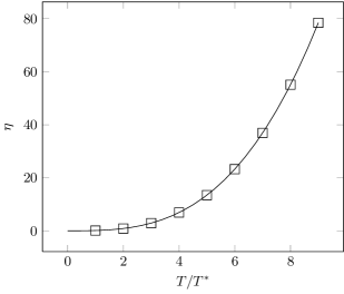
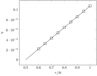
Figure 3: Shear viscosity $\eta$ as a function of the temperature with $T^{*}=100\text{ K}$. Here we have used $E_{1}=10^{-8}$, $E_{2}=0$, $\tau=\delta t$, and a system size of $64\times 64$. The solid line denotes the curve $\eta(x)=\frac{9\zeta(3)x^{3}}{32\pi}$.

Figure 4: Shear viscosity as function of the relaxation time $\tau$. Here we have used $E_{1}=10^{-8}$, $E_{2}=0$, $T_{0}=1$, and a system size of $64\times 64$. The solid line represents the curve $\eta(x)=\frac{9\zeta(3)}{16\pi}(x-0.5)$.

Note that rigid boundaries stem from a classical understanding of fluid dynamics, since in relativity the concept of solid walls is not well defined due to the Lorentz’s contraction. However, this effect is negligible as we are working in a reference frame with non-relativistic velocities and stationary walls.

IV.3 Thermal Conductivity Measurement

According to Ref. Cercignani and Kremer (2002) we can measure the heat-flux for processes close to equilibrium by considering the difference in the 3-velocities for the Eckart $U^{\alpha}$ and Landau-Lifschitz decomposition $U_{L}^{\alpha}$, i.e.

$$q^{\alpha}=(\epsilon+p)\left(U_{L}^{\alpha}-\frac{\langle p^{\alpha}\rangle}{n}\right)\text{ .}$$ (44)

For the measurement of the thermal conductivity, we use periodic boundary conditions in both directions and introduce a very small constant, homogeneous electric field into the system. As initial configuration, we choose a homogeneous temperature $T=T_{0}$ and zero energy flux. Therefore, we are dealing with a homogeneous situation, i.e. all spatial gradients vanish and a constant, homogeneous acceleration $\partial_{t}\vec{u}=-\frac{n\vec{E}}{\epsilon+p}$ is acting on the fluid components. According to the constitutive Eq. (9) the heat flux can be written as

$$\vec{q} =-\gamma\kappa T\partial_{t}\begin{pmatrix}\gamma u_{1}\\ \gamma u_{2}\end{pmatrix}\approx\frac{\kappa nT}{\epsilon+p}\begin{pmatrix}E_{1}\\ E_{2}\end{pmatrix}\text{ ,}$$

where for the last approximation we have assumed a non-relativistic charge flow, i.e. $|\vec{u}|/c\ll 1$. We find a constant, homogeneous heat flux $\vec{q}$. The temperature and relaxation time dependence of the heat conductivity are shown in Figs. 6 and 6. Expectedly, we cannot confirm $\kappa\propto\tau-\delta t/2$, but instead, we have found $\kappa\approx 1.525\tau T^{2}$. This is due to the fact that our model recovers only the first three moments of the equilibrium distribution, which are not sufficient to match all transport coefficients, in particular the thermal conductivity, given by theoretical predictions Mendoza et al. (2013). In the classical two-dimensional lattice Boltzmann simulation with a standard Bhatnager-Gross-Krook collision-operator Bhatnagar et al. (1954) one observes a similar effect when using the energy-conserving method from Ref. Ansumali and Karlin (2005), if the moments do not match up to fourth order.

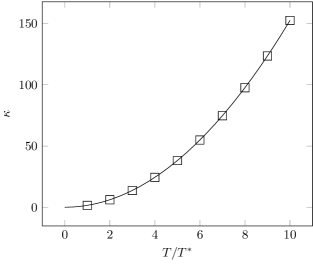
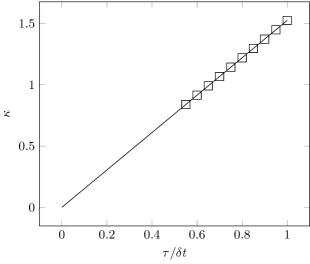
Figure 5: Thermal conductivity $\kappa$ as a function of the temperature at $t=10^{3}\delta t$ with $T^{*}=100\text{ K}$. The following values have been used: $E_{1}=10^{-8}$, $E_{2}=0$, $\tau=\delta t$, and a system size of $32\times 32$. The solid line is the fit: $\kappa(x)=1.525x^{2}$.

Figure 6: Thermal conductivity as a function of the relaxation time $\tau$ at $t=1000\delta t$. The following values have been used: $E_{1}=10^{-6}$, $E_{2}=0$, $T_{0}=1$, and a system size of $32\times 32$. The solid line denotes the curve given by the expression: $\kappa(x)=1.525x$.

IV.4 Stability Analysis

In analogy to the classical lattice Boltzmann simulations of the Rayleigh-Bénard instability Shan (1997), we include the unperturbed force density $\bar{n}e\bar{E}_{1}\hat{e}_{1}=-\vec{\nabla}V$ into the pressure term, i.e. $p\rightarrow p+V$, and could start the simulation with a homogeneous temperature distribution $T=T_{0}$ and zero energy flux. Since triggering an instability can be very complicated in numerical simulations, we have based our triggering mechanism on the method used in Ref. Shan (1997). Following this work, we proceed by changing the coefficients of the external force in Eqs. (41) and (42) by

$$b^{(01)} =\frac{b_{0}\langle p^{1}\rangle}{\langle p^{0}\rangle\Gamma_{F}^{(1)}T_{0}^{2}}\text{ ,}$$

$$b_{i}^{(10)} =\frac{2d_{0}(T/T_{0}-1)}{c_{10}\Gamma_{F}^{(0)}T^{2}_{0}}\delta_{i1}\text{ ,}$$

where the temperature distribution is calculated by

$$T=\frac{\pi^{2}}{18\zeta(3)}\frac{\epsilon}{n}\text{ .}$$

The new parameters stand for $b_{R}=\left(c_{V}\right)_{R}\beta_{R}$, and $d_{R}=\rho_{R}\left(\alpha_{q}\right)_{R}a_{R}$. Thus, the relativistic Rayleigh number reads

$$\mathrm{Ra}_{\text{rel}}=\frac{d_{R}b_{R}l^{4}}{\kappa_{R}\eta_{R}}\approx 3.047\frac{b_{0}d_{0}(l/\delta x)^{4}}{T_{0}^{5}\tau/\delta t(\tau/\delta t-1/2)}\text{ .}$$ (45)

Since, in our simulations, we are using the Landau-Lifschitz decomposition, it is not straightforward to impose the non- or transversal-conducting boundaries from Eqs. (28) to (31), and therefore, we approximate the non-conducting thermal boundaries by replacing the distribution function with the equilibrium value for $T=T_{0}$ and $\vec{u}_{L}=0$ at the edges in $x$-direction. In $y$-direction we choose periodic boundaries. The height of the system is chosen twice as long as the width, since according to Eq. (33) the critical wave length is $\lambda_{c}\approx 2.016l$. As initial condition, we start with a temperature distribution

$$T(x,y,t=0)=T_{0}\left[1+10^{-8}\frac{4x}{l}\left(1-\frac{x}{l}\right)\cos(k_{c}y)\right]\text{ .}$$

One observes the expected formation of convection cells with a wave length $\lambda\approx 2l$ and a cosine-shaped temperature perturbation, which vanishes at the thermal contacts, as shown in Fig. 7.

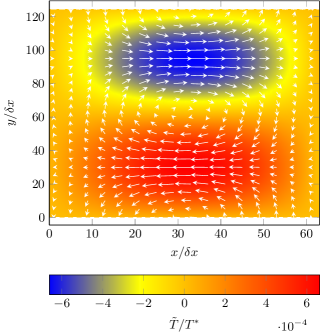
Figure 7: Electron velocity $\vec{u}/c$ and temperature perturbation field $\tilde{T}$ at $t=10^{5}\delta t$ with $T^{*}=100\text{ K}$. The simulation has been performed using a relaxation time $\tau=\delta t$, lattice temperature $T_{0}=1$, $b_{0}=d_{0}\approx 4.2\times 10^{-3}\Rightarrow\beta_{R}>0$, Rayleigh number $\mathrm{Ra}_{\text{rel}}=1800$, and a system size of $64\times 128$. Here $|\vec{u}/c|_{max}\sim 10^{-4}$.

As a next step, we use Eq. (45) to identify the critical Rayleigh number of our setup and compare it to our theoretical value, given by Eq. (32). This is done by measuring the logarithmic growth rate of the peak velocity of the charge flow perpendicular to the applied electric field $u_{2}$ at near-critical Rayleigh numbers, similar to the procedure described in Ref. Shan (1997). The maximum velocity is measured for $10^{-4}t\in\{6\delta t,9\delta t,\dots,30\delta t\}$. In Fig. (9) we see the exponential growth. In Fig. 9 we observe the linear dependence and measure a critical Rayleigh number of $\mathrm{Ra}_{c}\approx 1697$, which is about $0.6\%$ smaller than the theoretical value in Eq. (32). This shows that our numerical results have excellent agreement with our theoretical predictions.

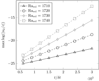
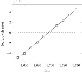
Figure 8: Logarithm of the peak vertical velocity as a function of time for a system size of $64\times 128$

Figure 9: Logarithmic growth rate as a function of the relativistic Rayleigh number for a system size of $64\times 128$ with dashed horizontal line at $y=0$

V Conclusion

We studied both, theoretically and numerically, the relativistic Rayleigh-Bénard instability for the charge transport in quantum critical graphene. As a new driving mechanism we introduced an electrical field to mimic the effects of the buoyancy force in the classical phenomenon, i.e. interchanging the role of mass and charge. We have found that the classical inhibitors (viscous forces and heat transport) and drivers (temperature gradient and external force) keep their role, and the instability can develop. Using a linear stability analysis, we derived a quantitative criterion ($\mathrm{Ra}_{\text{rel}}\geq\text{Ra}_{c}$) for the occurrence of the instability which compares the relativistic Rayleigh number of the system with the critical values in Eqs.  (32) and (34), whose magnitude depends on the nature of the boundary conditions. The ultra-relativistic fermionic plasma influences the formula for the relativistic Rayleigh number, but under the assumption of non-relativistic current flow it does not alter the critical Rayleigh number. Applying our result to graphene we have found that the experimental realization for the appearance of convection cells is challenging due to a large sample length of about $100\mu\text{m}$ but probably achievable in the near future. The reason for the large sample length are twofold. On one hand graphene’s high thermal conductivity supresses the instability. On the other hand we are constrained by the hydrodynamic regime of transport which limits the value for the charge density assuming a given average temperature where electron-electron and -hole collisions dominate over other scattering mechanisms. For the numerical simulations we have improved the method proposed in Ref. Öttinger et al. (2013), by adding an external force and determined the functional dependence of the transport coefficients on temperature and relaxation time. We have demonstrated the occurrence of the convection cell pattern with the expected critical wavelength and temperature distributions in the case of non-conducting boundaries. In addition, we have measured a critical relativistic Rayleigh number which is in very good agreement to our theoretical predictions from the stability analysis. Extending our theoretical results by analyzing non-Boussinesq effects, studying the influence of substrates, as e.g. $\mathrm{SiC}$, considering electron-phonon interactions on the instability, as well as applying our finding to thermo-electronic devices, will be a subject of future research.