The Low energy structure of the Nucleon-Nucleon interaction:
Statistical vs Systematic Uncertainties

Abstract

We analyze the low energy NN interaction by confronting statistical vs systematic uncertainties. This is carried out with the help of model potentials fitted to the Granada-2013 database where a statistically meaningful partial wave analysis comprising a total of $6713$ np and pp published scattering data from 1950 till 2013 below $350{\rm MeV}$ has been made. We extract threshold parameters uncertainties from the coupled channel effective range expansion up to $j\leq 5$. We find that for threshold parameters systematic uncertainties are generally at least an order of magnitude larger than statistical uncertainties. Similar results are found for np phase-shifts and amplitude parameters.

I Introduction

The goal of the present paper is to quantify the uncertainties on the knowledge of the NN system from the present available experimental pp and np scattering data and their uncertainties. We do this from a comprehensive partial wave analysis (PWA) containing the largest NN database to date wich permits a statistically self-consistent least squares fit. From the determination of several statistically equivalent interactions we deduce the residual systematic differences in many two body quantities of interest. The main result is the dominance of these systematic errors over the statistical ones determined from each interaction separately.

I.1 Uncertainties in the Nuclear Force

The NN interaction, as a key building block of nuclear physics, has traditionally been inferred from pp and np scattering data. This task is hampered both by the fragmentary body of experiments as well as by the incomplete status of the models used to analyze them. These aspects have important consequences regarding the predictive power, accuracy and precision in theoretical nuclear physics. In particular, ab initio calculations of nuclear structure and nuclear reactions in terms of protons and neutrons as elementary constituents require the design of Nucleon-Nucleon potentials validated with the existing scattering information (see e.g. Ref. Signell (1995) for a lucid presentation). As it is well known the form and representation of potentials is not unique, and the historic evolution reflects this large diversity (see Machleidt and Li (1994) and references therein for a pre-nineties review). Even if a set of potentials are succesfully validated against the existing scattering data by an statistically acceptable $\chi^{2}$ fit value, the inferred predictions of unmeasured scattering quantities or other observable quantities such as nuclear bindings have two sources of uncertainties. Besides the obvious ones stemming from the experimental data and whose statistical nature requires passing elementary statistical tests, one also has a dependence on the particular choice of potential used to make the fit. This residual non-statistical dependence is our definition of the systematic uncertainty. In what follows we will ellaborate on what we think are elementary aspects of error analysis Evans and Rosenthal (2004), as applied to the NN interaction since these basic principles can be easily implemented in large scale fits and calculations.

The statistical uncertainties are easier to quantify, provided one can credibly establish that the discrepancies between theory and experiment are fluctuations whose probability distribution is either known a priori or confidently tested a posteriori. For the conventional least squares $\chi^{2}$-fit procedure this corresponds to test the normality of fitting residuals obtained by building the differences from the optimized theory and the fitted experimental data. When this is the fortunate case, the fit is self-consistent as the a priori assumption is verified a posteriori by the actual fit, and statistical error propagation can routinely be undertaken. We stress this essential point as it has too often been ignored in the design of the so-called high-quality potentials in the past.

Systematic uncertainties are notoriously more difficult to pin down in general. In fact, there are many ways to quantify the systematic uncertainties and none of them can be complete within the present context for two main reasons. On the one hand there are many imaginable forms of potentials which could fit the existing finite amount of data with equal statistically meaningfull quality, and thus in general only lower bounds on the systematics can be estimated. On the other hand there exist many derived quantities such as scattering amplitudes, phase-shifts or nuclear binding energies which will reflect the effect of the systematic error differently on a quantitative level. This has been the traditional approach to systematic uncertainties in the past by trying out different high quality potentials in nuclear structure ab initio calculations (see e.g. Maris et al. (2009); Coraggio et al. (2009); Bogner et al. (2010); Roth et al. (2010); Leidemann and Orlandini (2013); Marcucci et al. (2016); Navratil et al. (2016)).

I.2 Our contribution to NN analyses

Our work can be framed within the currently growing efforts to realistically pin down the existing uncertainties stemming from different sources in theoretical nuclear physics Dudek et al. (2013); Dobaczewski et al. (2014). In fact, a special issue dedicated to this topic appeared recently in Jour. Phys. G Ireland and Editors) (2015) . In this paper we will restrict the analysis to the NN scattering amplitude and try to set lower bounds both on statistical as well as systematic uncertainties in terms of a finite number of potentials suitable for nuclear structure calculations. The set of model potentials used below is a convenient tool with the purpose of quantifying the uncertainties. This is a necessary but already insightful step before extending these uncertainties to ab initio nuclear structure calculations. Since it is naturally assumed that for light nuclei nuclear binding is mainly sensitive to low energy NN scattering, we also extensively study the long wavelength limit because also potential model details are expected to become least relevant. We find that even in the low energy limit the systematic uncertainties dominate over those statistical uncertainties arising directly from the same experimental data. Our analysis is based on a comparison of 6 statistically acceptable but different model potentials, i.e., with $\chi^{2}/{\rm d.o.f}\sim 1$ developed by our group fitting the same self consistent Granada database comprising a total of 6713 NN scattering Navarro Pérez et al. (2013a). The present paper is complementary to Navarro Pérez et al. (2013a) and further dedicated studies along these lines Navarro Pérez et al. (2014a, 2015a).

I.3 The NN error analysis in retrospect

In order to understand our most unexpected result and to provide a proper perspective, we provide at this point a sucint review with the historic benchmarks as guidelines highlighting those aspects specifically dealing with our work. We recommend the comprehensive presentation covering up to 1992 for a wider scope Machleidt and Li (1994).

The low energy structure of the NN interaction has received a recurrent attention since the late 40’s when Bethe proposed the effective range expansion Bethe (1949) (ERE). The shape and model independence of the amplitude captured with a few number of parameters the essence of the NN force; an unique and particularly appealing universal pattern in the long wavelength limit of short range interactions. Because this is a low energy expansion of the full scattering amplitude in powers of small momentum, higher partial waves are not needed in principle, and one may imagine an ideal situation with a direct determination from very low energy scattering only. However, these very low energy data are scarce and an extrapolation to zero energy must always be made. Much higher accuracy can be obtained by intertwining lower and higher energies via a large scale Partial Wave Analysis (PWA) so that many more data contribute to the threshold parameters precision when the resulting scattering amplidues are evaluated at zero energy. While this procedure largely increases the statistics, this interrelation cannot be achieved for free. As we discuss next some unavoidable model dependence is introduced, thus generating a source of systematic errors beyond the genuine statistical errors of the PWA.

Indeed, the NN scattering amplitude contains 10 functions of energy and angle and a complete set of experiments is needed to determine it without model dependence Puzikov et al. (1957). While the usefulness of polarization was soon realized Schumacher and Bethe (1961) as well as the strong unitarity constraints on the uniqueness of the solution Alvarez-Estrada et al. (1973); Bystricky et al. (1978) (see  Kamada et al. (2011) for an analytical solution), complete sets of observables are scarce at the energies relevant to nuclear structure applications, corresponding to energies below or about pion production threshold (see also Arndt and Roper (1972)). Following the standard custom, we will take the maximal LAB energy in our potential analysis to be $350{\rm MeV}$, which has been the canonical choice for NN potential fits. As a consequence a PWA in conjunction with the standard least squares $\chi^{2}$-method pioneered by Stapp and Ypsilantis Stapp et al. (1957) is usually pursued to fit the set of measured scattering observables at given discrete energy and angle values. Soon thereafter, the nowadays widely accepted probabilistic interpretation of the $\chi^{2}$-fit in terms of the p-value was introduced as a measure of the confidence level Cziffra et al. (1959); MacGregor et al. (1959) (see particularly the figure in MacGregor et al. (1959) where the p-value is explicitly displayed). The method was popularized during the 60’s by MacGregor and Arndt with additional implementations, such as a rejection criterium for the growing number of incompatible parameters Arndt and MacGregor (1966); Arndt and Macgregor (1966); MacGregor et al. (1968). This is nothing but the long established Chauvenet’s $3\sigma$ criterion (see Taylor (1997)) to statistically reject data sets with an improbably high or improbably low $\chi^{2}$ value.

This incomplete and discretized experimental information requires using smooth interpolating energy dependent functions for the scattering matrix in all partial waves for nearby but unmeasured kinematic regions. Alternatively, quantum mechanical potentials with proper long distance behavior generate analytical energy dependence with the adequate cut-structure in the complex energy plane (see e.g. Ref. Signell (1995) for a review). We follow here the potential approach since it has the obvious advantage over a mere partial wave analysis of being of direct use in nuclear structure calculations, and hence it allows to direct transporting uncertainties from the data to energy bindings. The potential approach is subjected to inverse scattering off-shell ambiguities Chadan and Sabatier (2011) as the potential contains generically 10 matrix functions Okubo and Marshak (1958), manifesting themselves as a systematic uncertainty in the observables at the interpolated, not directly measured, energy values. If one fixes a maximum energy for the PWA the ambiguities reflect the finite spatial resolution corresponding to the shortest de Broglie wavelength below which the interaction is not determined by the data. Thus, we might expect that in the long wavelength limit systematic uncertainties will be greatly reduced.

I.4 Organization of the paper

The paper is organized as follows. In Section II we describe the main ideas behind our analysis, reviewing our previous works as well as a summary of the 6 model potentials used in our analysis. We remind the effective range expansion for the deuteron channel in Section III. The convenient and accurate tool which we will be using to evaluate low energy parameters in the discrete version of the coupled channel variable S-matrix approach is presented in Section C. This framework proves extremely convenient to discuss the pertinent sampling of the interaction, and the difference between fine and coarse graining is addressed in Section IV. There, peculiar numerical aspects of these calculations are also analyzed. Our main numerical results concerning the comparison between statistical vs systematic uncertainties are presented in Section V in terms of phase-shifts, scattering amplitudes and potentials. In Section VI we ponder on the portability of phase shift analyses based on our own experience with nuclear potentials. Finally, in Section VII we summarize our main results and conclusions. In the appendices we provide some details concerning three new potentials introduced in the present work.

II NN Data, Models and Uncertainties

Table 1: Model Potentials Summary.

Potential	Number of Parameters	$N_{np}$	$N_{pp}$	$\chi^{2}_{np}$	$\chi^{2}_{pp}$	$\chi^{2}/{\rm d.o.f.}$	p-value	Gaussianity	Birge Factor
DS-OPE	46	2996	3717	3051.64	3958.08	1.05	0.32	Yes	1.03
DS-$\chi$TPE	33	2996	3716	3177.43	4058.28	1.08	0.50	Yes	1.04
DS-$\Delta$BO	31	3001	3718	3396.67	4076.43	1.12	0.24	Yes	1.06
Gauss-OPE	42	2995	3717	3115.16	4048.35	1.07	0.33	Yes	1.04
Gauss-$\chi$TPE	31	2995	3717	3177.22	4135.02	1.09	0.23	Yes	1.05
Gauss-$\Delta$BO	30	2995	3717	3349.89	4277.58	1.14	0.20	Yes	1.07

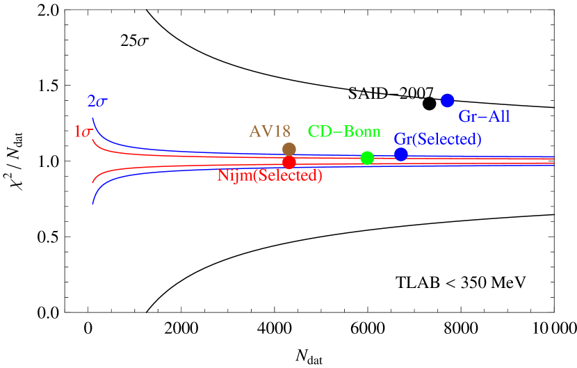
Figure 1: Values of the $\chi^{2}/N_{\rm dat}$ as a function of the number of data $N_{\rm dat}$ provided by the experimentalists for several fits at LAB energies below $350$MeV. We include the Nijmegen PWA Stoks et al. (1993), the AV18 potential Wiringa et al. (1995) the CD-Bonn potential Machleidt (2001), the Granada PWA Navarro Pérez et al. (2013b) and the SAID PWA Briscoe et al. . In the Granada analysis we distinguish between a fit to all the published data (Gr-All) and the $3\sigma$ self-consistent database, Gr(Selected). For comparison we also plot the $1\sigma$, $2\sigma$ and $25\sigma$ confidence levels.

II.1 The situation after the Nijmegen-1993 analysis

The description of NN scattering data by phenomenological potentials started in the mid-fifties Stapp et al. (1957) and has been pursued ever since (see Machleidt and Li (1994) and references therein for a pre-nineties review). However a successful fit, determined by the merit figure $\chi^{2}/{\rm d.o.f}\sim 1$, was not achieved until 1993 when the Nijmegen group applied in this context Chauvenet’s $3\sigma$ rejection criterion already proposed in 1968 MacGregor et al. (1968) to statistically discard data sets with an improbably high or improbably low $\chi^{2}$ value  Stoks et al. (1993).

In Fig. 1 we illustrate the situation for $\chi^{2}/N_{\rm dat}$. The number of data is so large that the $\chi^{2}$-distribution behaves as a normal distribution with mean value $\nu$ and variance $2\nu$ Taylor (1997). In addition, $\nu\simeq N_{\rm dat}$, since the number of fitting parameters is usually much less than $N_{\rm dat}$. Thus, the mean and variance of the reduced distribution, $\chi^{2}/\nu$, are $1$ and $\sqrt{2/\nu}$ respectively. Therefore those fits in Fig. 1 falling outside the interval $1\pm N\sqrt{2/N_{\rm dat}}$ contain gross systematic errors with a $68\%,95\%$ confidence level for $N=1,2$ respectively. For instance, for the SAID database Briscoe et al. the total number of data is $N_{\rm dat}=3075_{pp}+4159_{np}=7234$ and the total $\chi^{2}=4043_{pp}+6160_{np}=10203$, giving $\chi^{2}/N_{\rm dat}=1.4157$. Then, $\sigma=\sqrt{2/7234}=0.017$. Thus, the SAID reduced $\chi^{2}$-value is $1.41=1+25\sigma$. This value is probably so large because the full database has been used before the data selection. More recent chiral motivated interactions usually fit data up to lower energies Gezerlis et al. (2014); Entem and Machleidt (2003) and are therefore in this picture. However, some of their merits have been discussed on previous publications Navarro Pérez et al. (2015b, 2016a).

After this first statistically satisfactory Nijmegen study, several potentials describing data up to a laboratory frame energy of $350$ MeV were developed with similar $\chi^{2}/{\rm d.o.f}$ values. All of them include the distinguished charge dependent (CD) one pion exchange (OPE), magnetic moments, vacuum polarization and relativistic effects as the long range part of the interaction, and around $40$ parameters for the short and intermediate range regions Stoks et al. (1993, 1994); Wiringa et al. (1995); Machleidt (2001); Gross and Stadler (2008). These OPE-tailed potentials with $\chi^{2}/{\rm d.o.f}\lesssim 1$ have played a major role in nuclear physics. It should be noted, however, that an error analysis of these potentials based on the finite experimental scattering accuracy has been overlooked, and as a consequence any ab initio nuclear structure calculations using them are unable to quantify the impact of NN scattering uncertainties in nuclear bindings.

II.2 Granada-2013 database and Potentials

In a recent paper we have updated the Nijmegen PWA by including data up to 2013, improving after Gross and Stadler (2008) the $3\sigma$ criterion to select a self-consistent database with $N=6713$ np and pp scattering data and providing statistical error bars to the fitting parameters Navarro Pérez et al. (2013b, a). The self-consistent Granada database is available for download Navarro Pérez et al. (2013c). The delta-shell (DS) representation of the potential allowed the propagation of statistical uncertainties from the scattering data into potential parameters, phase shifts, scattering amplitudes and deuteron properties. This was possible due to the simplification in calculating the Hessian matrix. Subsequently, we have extended the DS potential including chiral two pion exchange ($\chi$TPE) in the intermediate and long range regions Navarro Pérez et al. (2014b, c). We also introduced a local, smooth potential parameterized as a sum of Gaussians (SOG) with OPE Navarro Pérez et al. (2014a). In appendices A.1 and A.2 we introduce three new model interactions. One of them is a SOG model with $\chi$TPE. The other two contain $\Delta$ resonances as dynamical degrees of freedom through the Born-Oppenheimer approximation ($\Delta$BO), and are modeled either by DS or SOG at short distances. Note that only the SOG model potentials are smooth and can be plotted. The statistical features of the 6 model interactions are displayed in Table 1 where we provide the number of Parameters for np and pp scattering, , $N_{np}$ and $N_{pp}$ respectively, as well as the total $\chi^{2}$ values in each separate case. The p-value corresponds to the actual $\chi_{\rm min}^{2}/\nu$ value. As we have stressed in our previous works Navarro Pérez et al. (2014a, 2015a) one can globally sligthtly enlarge the experimental uncertainties by the so-called Birge factor provided the residuals pass a gaussianity test. After this re-scaling the p-value becomes 0.68 for a $1\sigma$ confidence level and hence all potentials become statistically equivalent. As can be seen all of our potentials incorporate the appropriate propagation of statistical uncertainties. This has been possible because the residuals of our fits are normally distributed. This requirement of the $\chi^{2}$ method, has been verified a posteriori with a high confidence level. We stress that a lack of normality in the residuals would strongly suggest the presence of systematic uncertainties in the analysis, disallowing the propagation of statistical errors. The same database has also been recently used to fit a chiral TPE potential that directly includes delta excitation Piarulli et al. (2015). In the cases where normality is unequivocally fulfilled we have propagated statistical uncertainties by applying the bootstrap Monte Carlo method directly to the experimental data Navarro Pérez et al. (2014d), which simulates an ensemble of conceivable experiments based on the experimental uncertainties estimates. A similar method has successfully been applied to estimate the statistical uncertainty in the triton binding energy solving the Faddeev equations Navarro Pérez et al. (2014e) and the alpha-particle using shell model techniques Navarro Pérez et al. (2015c). A similar propagation to the $\alpha$-particle binding energy solving the Faddeev-Yakubovsky equations Navarro Pérez et al. (2016b) has been advanced recently.

In Fig. 1 the $N\sigma$ confidence level corresponds to the interval $\chi^{2}/N_{\rm dat}=1\pm N\sqrt{2/N_{\rm dat}}$ and the corresponding p-value is $p=1-\int_{-N}^{N}dxe^{-x^{2}/2}/\sqrt{2\pi}$. The p-value is the probability of being wrong when denying the normal nature of the fluctuations. Both the SAID fit Briscoe et al. and the Granada-All fit provide a similar value which is outside a $25\sigma$ band, which implies a p-value smaller than $10^{-10}$. As we discussed in detail in our previous work, one can tolerate a value of $\chi^{2}/N_{\rm dat}$ outside the interval $1\pm\sqrt{2/N_{\rm dat}}$ as long as we can identify a scaled gaussian distribution by using normality tests. Navarro Pérez et al. (2015a). As it was pointed out  Navarro Pérez et al. (2015a) this is not the case for the Granada-All database, and thus the selection of data seems mandatory . From the figure it is also clear that the self-consistent Granada-2013 database is so far the largest database consistent with a statistically successfull PWA of np and pp scattering below LAB energy $350{\rm MeV}$.

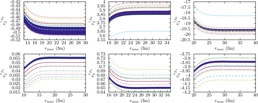
Figure 2: Convergence of the ${}^{1}S_{0}$ and ${}^{3}S_{1}$ low energy threshold parameters $v_{2}$, $v_{3}$ and $v_{4}$ as a function of the integration distance and for the DS-OPE Navarro Pérez et al. (2013b, a) (blue band), DS-$\chi$TPE Navarro Pérez et al. (2014b, c) (dashed red line), Gauss-OPE Navarro Pérez et al. (2014a) (dotted green line), Gauss-$\chi$TPE (dotted light green line), DS-$\Delta$BO (dotted purple line), Gauss-$\Delta$BO (dotted dashed ligth yellow line), NijmII Stoks et al. (1994) (dotted olive green line), Reid93 Stoks et al. (1994) (dotted dashed light blue line) and AV18 Wiringa et al. (1995) (dotted dashed light red line). The width of the blue band reflects the corresponding statistical error estimate.

III Low energy expansion

As already mentioned, in the absence of complete sets of measurements one must resort to specific potentials to carry out the PWA. Since the form of the potential is chosen and fixed a priori, the analysis of NN scattering data is subjected to inverse scattering ambiguities which are amplified as the energy increases. Therefore one expects lowest energy information to be more universal and thus we use the effective range expansion (ERE) Bethe (1949) as the suitable tool. Although for S-waves the calculation of the low energy threshold parameters is straightforward and even customary for NN potentials, their calculation for higher and coupled channel partial waves is a computational challenge which has seldomly been addressed. To start with, there are not even ready-to-use formulas in the coupled channel case, and a low energy expansion of the wave function to high orders is needed. In addition, partial waves with high angular momentum become numerically unstable as the main contribution comes from very long distances requiring demanding numerical computations. This is the reason why these low energy parameters have been very rarely computed or, when they have been, a very limiting accuracy has been displayed. Using Calogero’s variable phase approach to the full S-matrix Calogero (1967) the low energy parameters have only been calculated for the Reid93 and NijmII potentials up to $j\leq 5$ Pavon Valderrama and Ruiz Arriola (2005). Here we improve on the accuracy of that work and determine for the first time the statistical uncertainties of the low energy threshold parameters. The method to compute these low energy parameters in the general case is based on the discrete variable-S-matrix method which we explain in more detail in Appendix C. In essence in this method one replaces the original potential by a sum of delta-shells, which in the equidistant case corresponds to $U(r)\to\sum_{i=1}U(r_{i})\delta(r-r_{i})\Delta r$ and computes the accumulated phase of S-matrix es the number of grid points is switched on. The low energy parameters for higher partial waves determined in Ref. Pavon Valderrama and Ruiz Arriola (2005) have been used to implement renormalization conditions Ruiz Arriola (2010); Pavon Valderrama (2011); Long and Yang (2011, 2012) and to analyze causality bounds in np scattering Elhatisari and Lee (2012).

In the well known case of central ${}^{1}S_{0}$ and ${}^{3}S_{1}$ partial waves the ERE is given by (using the nuclear bar representation)

$$k\cot\delta_{0}=-\frac{1}{\alpha_{0}}+\frac{1}{2}r_{0}k^{2}+v_{2}k^{4}+v_{3}k^{6}+v_{4}k^{8}+\ldots,$$ (1)

where $k$ is the center of mass momentum, $\delta_{0}$ is the corresponding partial wave phase-shift, $\alpha_{0}$ is the scattering length, $r_{0}$ is the effective range and $v_{i}$ are known as the curvature parameters. The generalization to N-coupled partial waves with angular momenta $(l_{1},\cdots,l_{N})$ can be done by introducing the $\mathbf{\hat{M}}$ matrix defined as

$$\mathbf{DSD}^{-1}=\left(\mathbf{\hat{M}}+ik\mathbf{D}^{2}\right)\left(\mathbf{\hat{M}}-ik\mathbf{D}^{2}\right)^{-1},$$ (2)

where $\mathbf{S}$ is the usual unitary S-matrix and $\mathbf{D}={\rm diag}(k^{l_{1}},\ldots,k^{l_{N}})$. In the limit $k\to 0$ the $\mathbf{\hat{M}}$-matrix becomes

$$\mathbf{\hat{M}}=-\mathbf{a}^{-1}+\frac{1}{2}\mathbf{r}k^{2}+\mathbf{v_{2}}k^{4}+\mathbf{v_{3}}k^{6}+\mathbf{v_{4}}k^{8}+\dots,$$ (3)

where $\mathbf{a}$, $\mathbf{r}$ and $\mathbf{v_{i}}$ are the coupled channel generalizations of $\alpha_{0}$, $r_{0}$ and $v_{i}$ respectively. Due to $n\pi$ exchange $\mathbf{\hat{M}}(k)$ has branch cuts at $k=\pm inm_{\pi}/2$, and thus the ERE converges for $|k|<m_{\pi}/2$ or $E_{\rm LAB}\lesssim 10{\rm MeV}$. Conversely, the ERE to finite order does not allow to reconstruct the full functions in the complex plane without the explicit cut structure information.

In the NN case these matrices have dimension 1 and 2. We refer to Ref. Pavon Valderrama and Ruiz Arriola (2005) for further details. In the interesting case of the ${}^{3}S_{1}$ eigen-channel, one has 

$$k\cot\delta_{3S1}^{\rm Eigen}=-\frac{1}{\alpha_{3S1}^{\rm Eigen}}+\frac{1}{2}r_{3S1}^{\rm Eigen}k^{2}+v_{3S1}^{\rm Eigen}k^{4}+\dots$$ (4)

where we get for the effective range parameters the relations between the eigen and the nuclear bar (denoted emphatically as barred) representations,

$$\alpha_{3S1}^{\rm Eigen} = \bar{\alpha}_{3S1}$$ (5)

$$r_{3S1}^{\rm Eigen} = \bar{r}_{3S1}+\frac{2\bar{r}_{E1}\bar{\alpha}_{E1}}{\bar{\alpha}_{3S1}}+\frac{\bar{r}_{3D1}\bar{\alpha}_{E1}^{2}}{\bar{\alpha}_{3S1}^{2}}$$ (6)

$$v_{3S1}^{\rm Eigen} = \bar{v}_{3S1}+\frac{1}{4}\bar{\alpha}_{3D1}\bar{r}_{E1}^{2}$$ (7)

$$+ \frac{\bar{\alpha}_{E1}}{4\bar{\alpha}_{3S1}}\left(2\bar{\alpha}_{3D1}\bar{r}_{3D1}\bar{r}_{E1}-\bar{\alpha}_{E1}\bar{r}_{E1}^{2}+8\bar{v}_{E1}\right)$$

$$+ \frac{\bar{\alpha}_{E1}^{2}}{4\bar{\alpha}_{3S1}^{2}}\left(\bar{\alpha}_{3D1}\bar{r}_{3D1}^{2}-2\bar{\alpha}_{E1}\bar{r}_{3D1}\bar{r}_{E1}+4\bar{v}_{3D1}\right)$$

$$+ \frac{1}{4\bar{\alpha}_{3S1}^{3}}\left(4\bar{\alpha}_{E1}^{2}-\bar{\alpha}_{E1}^{4}\bar{r}_{3D1}^{2}\right)$$

and so on.

Table 2: Low-energy scattering parameters for the ${}^{3}S_{1}$ eigen-phase. We quote the numbers of Ref. de Swart et al. (1995) for the PWA Stoks et al. (1993) and the Nijm-I, Nijm-II and Reid 93 potentials Stoks et al. (1994), (first four rows), our results integrating the discrete variable S-matrix equations with $N=2\times 10^{5}$ grid points for the Nijm-II and Reid 93 Stoks et al. (1994) and AV18 Wiringa et al. (1995) potentials quoting numerical errors (in boldface) relative to the computation with $N=1\times 10^{5}$. Statistical errors are also quoted when available.

	$\alpha_{0}$	$r_{0}$	$v_{2}$	$v_{3}$	$v_{4}$
PWA	5.420(1)	1.753(2)	0.040	0.672	–3.96
Nijm I	5.418	1.751	0.046	0.675	–3.97
Nijm II	5.420	1.753	0.045	0.673	–3.95
Reid93	5.422	1.755	0.033	0.671	–3.90
NijmII	5.4197(3)	1.75343(3)	0.04545(1)	0.6735(1)	–3.9414(8)
Reid93	5.4224(2)	1.75550(3)	0.03269(1)	0.6721(1)	–3.8867(7)
AV18	5.4020(2)	1.75171(3)	0.03598(1)	0.6583(1)	–3.8507(7)
DS-OPE	5.435(2)	1.774(3)	0.055(1)	0.650(2)	–3.84(1)
DS-TPE	5.424	1.760	0.050	0.666	–3.90
DS-$\Delta$BO	5.419	1.752	0.046	0.672	–3.93
G-OPE	5.441	1.781	0.056	0.642	–3.80
G-TPE	5.410	1.739	0.040	0.681	–4.01
G-$\Delta$BO	5.397	1.722	0.030	0.693	–4.06

Table 3: Low energy threshold np parameters for all partial waves with $j\leq 5$. The central value and statistical error bars are given on the first line of each partial wave and correspond to the mean and standard deviation of a population of $1020$ parameters calculated with the Monte Carlo family of potential parameters described in Navarro Pérez et al. (2014d) using the DS-OPE potential Navarro Pérez et al. (2013b, a). The second line quotes the systematic uncertainties, the central value and error bars correspond to the mean and standard deviation of the 9 realistic potentials NijmII Stoks et al. (1994), Reid93 Stoks et al. (1994), AV18 Wiringa et al. (1995), DS-OPE Navarro Pérez et al. (2013b, a), DS-$\chi$TPE Navarro Pérez et al. (2014b, c), Gauss-OPE Navarro Pérez et al. (2014a), Gauss-$\chi$TPE, DS-$\Delta$BO and Gauss-$\Delta$BO. For each partial wave we show the scattering length $\alpha$ and the effective range $r_{0}$, both in ${\rm fm}^{l+l^{\prime}+1}$, as well as the curvature parameters $v_{2}$ in ${\rm fm}^{l+l^{\prime}+3}$, $v_{3}$ in ${\rm fm}^{l+l^{\prime}+5}$ and $v_{4}$ in ${\rm fm}^{l+l^{\prime}+5}$. For the coupled channels we use the nuclear bar representation of the $S$ matrix. Uncertainties smaller than $10^{-3}$ are not quoted

Wave	$\alpha$	$r_{0}$	$v_{2}$	$v_{3}$	$v_{4}$
${}^{1}S_{0}$	$-23.735(6)$	$2.673(9)$	$-0.50(1)$	$3.87(2)$	$-19.6(1)$
	$-23.735(16)$	$2.68(3)$	$-0.48(2)$	$3.9(1)$	$-19.6(5)$
${}^{3}P_{0}$	$-2.531(6)$	$3.71(2)$	$0.93(1)$	$3.99(3)$	$-8.11(5)$
	$-2.5(1)$	$3.7(4)$	$0.9(5)$	$3.9(1)$	$-8.2(9)$
${}^{1}P_{1}$	$2.759(6)$	$-6.54(2)$	$-1.84(5)$	$0.41(2)$	$8.39(9)$
	$2.78(3)$	$-6.46(9)$	$-1.7(2)$	$0.5(2)$	$8.0(3)$
${}^{3}P_{1}$	$1.536(1)$	$-8.50(1)$	$0.02(1)$	$-1.05(2)$	$0.56(1)$
	$1.52(1)$	$-8.6(1)$	$-0.06(7)$	$-0.9(2)$	$0.1(5)$
${}^{3}S_{1}$	$5.435(2)$	$1.852(2)$	$-0.122(3)$	$1.429(7)$	$-7.60(3)$
	$5.42(1)$	$1.84(1)$	$-0.14(1)$	$1.46(3)$	$-7.7(2)$
$\epsilon_{1}$	$1.630(6)$	$0.400(3)$	$-0.266(5)$	$1.47(1)$	$-7.28(2)$
	$1.61(2)$	$0.39(2)$	$-0.29(3)$	$1.47(2)$	$-7.35(9)$
${}^{3}D_{1}$	$6.46(1)$	$-3.540(8)$	$-3.70(2)$	$1.14(2)$	$-2.77(2)$
	$6.43(4)$	$-3.57(2)$	$-3.77(4)$	$1.11(5)$	$-2.7(1)$
${}^{1}D_{2}$	$-1.376$	$15.04(2)$	$16.68(6)$	$-13.5(1)$	$35.4(1)$
	$-1.379(6)$	$15.00(9)$	$16.7(2)$	$-12.9(4)$	$36.2(14)$
${}^{3}D_{2}$	$-7.400(4)$	$2.858(3)$	$2.382(9)$	$-1.04(2)$	$1.74(2)$
	$-7.39(1)$	$2.87(1)$	$2.41(3)$	$-0.96(5)$	$1.75(8)$
${}^{3}P_{2}$	$-0.290(2)$	$-8.19(1)$	$-6.57(5)$	$-5.5(2)$	$-12.2(3)$
	$-0.288(5)$	$-8.3(2)$	$-6.8(7)$	$-6.1(19)$	$-12.7(26)$
$\epsilon_{2}$	$1.609(1)$	$-15.68(2)$	$-24.91(8)$	$-21.9(3)$	$-64.1(7)$
	$1.604(6)$	$-15.8(2)$	$-25.2(7)$	$-23.0(29)$	$-66.2(69)$
${}^{3}F_{2}$	$-0.971$	$-5.74(2)$	$-23.26(8)$	$-79.5(4)$	$-113.0(16)$
	$-0.971(5)$	$-5.7(1)$	$-23.3(6)$	$-80.1(33)$	$-117.2(121)$
${}^{1}F_{3}$	$8.378$	$-3.924$	$-9.869(4)$	$-15.27(2)$	$-1.95(7)$
	$8.377(5)$	$-3.926(4)$	$-9.88(2)$	$-15.3(1)$	$-2.2(4)$
${}^{3}F_{3}$	$2.689$	$-9.978(3)$	$-20.67(2)$	$-19.12(8)$	$-27.7(2)$
	$2.690(6)$	$-9.97(2)$	$-20.65(8)$	$-19.0(3)$	$-26.9(7)$
${}^{3}D_{3}$	$-0.134$	$1.373$	$2.082(3)$	$1.96(1)$	$-0.45(3)$
	$-0.14(2)$	$1.371(3)$	$2.07(1)$	$1.92(6)$	$-0.51(9)$
$\epsilon_{3}$	$-9.682$	$3.262$	$7.681(3)$	$9.62(2)$	$-1.09(5)$
	$-9.683(5)$	$3.260(5)$	$7.67(2)$	$9.6(1)$	$-1.1(2)$
${}^{3}G_{3}$	$4.876$	$-0.027$	$0.019(2)$	$0.07(1)$	$-2.69(3)$
	$4.875(3)$	$-0.03(1)$	$-0.01(6)$	$-0.05(30)$	$-2.8(7)$
${}^{1}G_{4}$	$-3.208$	$10.833(1)$	$34.629(9)$	$83.04(8)$	$108.1(4)$
	$-3.212(6)$	$10.81(2)$	$34.53(7)$	$82.4(4)$	$105.6(15)$
${}^{3}G_{4}$	$-19.145$	$2.058$	$6.814$	$16.769(4)$	$10.00(2)$
	$-19.147(8)$	$2.058$	$6.815(3)$	$16.78(2)$	$10.04(6)$
${}^{3}F_{4}$	$-0.006$	$-3.043$	$-4.757(1)$	$73.903(5)$	$662.21(9)$
	$-0.010(2)$	$-3.044(8)$	$-4.77(5)$	$73.9(3)$	$662.8(32)$
$\epsilon_{4}$	$3.586$	$-9.529$	$-37.02(3)$	$-184.40(2)$	$-587.28(9)$
	$3.589(8)$	$-9.53(2)$	$-37.04(7)$	$-184.6(3)$	$-586.6(17)$
${}^{3}H_{4}$	$-1.240$	$-0.157(2)$	$-1.42(1)$	$-14.0(1)$	$-99.0(9)$
	$-1.241(3)$	$-0.18(1)$	$-1.55(9)$	$-15.2(8)$	$-106.7(55)$
${}^{1}H_{5}$	$28.574$	$-1.727$	$-7.906$	$-32.787$	$-59.361$
	$28.58(1)$	$-1.727$	$-7.906(4)$	$-32.78(2)$	$-59.38(5)$
${}^{3}H_{5}$	$6.081$	$-6.439$	$-25.228$	$-82.511(3)$	$-168.47(2)$
	$6.09(2)$	$-6.44(1)$	$-25.22(5)$	$-82.5(1)$	$-168.3(8)$
${}^{3}G_{5}$	$-0.008$	$0.481$	$1.878$	$6.100$	$6.791$
	$-0.009(1)$	$0.480$	$1.878$	$6.098(3)$	$6.784(9)$
$\epsilon_{5}$	$-31.302$	$1.556$	$6.995$	$28.179$	$48.376(2)$
	$-31.31(1)$	$1.556$	$6.993(3)$	$28.17(1)$	$48.35(3)$
${}^{3}I_{5}$	$10.678$	$0.011$	$0.146$	$1.441$	$6.546(6)$
	$10.680(5)$	$0.011$	$0.145(1)$	$1.43(1)$	$6.47(9)$

IV Sampling the NN interaction: Fine graining vs Coarse graining

Several high-quality interactions stemming from the 1993 Nijmegen PWA such as the NijmII, Reid93, AV18 potentials are smooth functions in configuration space. For the discrete S-matrix method (see Appendix C for details) this means that the values $U(r_{i})$ are given for $U=U_{\rm NijmII},U_{\rm Reid93},U_{\rm AV18}$, and thus a fine graining $\Delta r\to 0$ is needed. We test the numerical accuracy and precision of the approach by using a finite grid representation and determine the low energy parameters of these potentials. In particular, we take $r_{\rm max}=100\,{\rm fm}$ and $\Delta r=0.01,0.005,0.001,0.0005\,{\rm fm}$ corresponding to $N=1\times 10^{4},2\times 10^{4},10^{5},2\times 10^{5}$ grid points respectively and convergence is established for both $\Delta r$ and $r_{\rm max}$.

For illustration we show in Fig. 2 eye-ball convergence for $v_{2,3,4}$ (eigen) in the ${}^{3}S_{1}$ channel, which is achieved with an integration upper limit of $r_{\rm max}=30-40{\rm fm}$. Sufficiently high numerical convergence is comfortably obtained with $r_{\rm max}=100{\rm fm}$ for all partial waves with $J\leq 5$.

In order to gauge the accuracy of our calculation we compare with the last revision of the Nijmegen group de Swart et al. (1995). In table 2 we show our results computed with the DVSM method. As we see, our implementation allows for high numerical precision which can be tuned to be the highest one among other sources of uncertainties, namely statistical and systematic errors to be discussed below. If we take the quoted numbers in Ref. de Swart et al. (1995) as significant figures, and assuming the standard round-off error rules, their numerical error is smaller than a half of the last provided digit. Our results are mostly compatible with theirs but considerably more precise.

It is useful to ponder on our numerical accuracy by looking into other possible integration methods. In the conventional Numerov of Runge-Kutta methods, usually employed for smooth potentials, convergence is defined in terms of the precision of the wave function, so that one needs a large number of mesh-points. The accuracy is also an issue in momentum space calculations where the momentum grid has an ultraviolet cut-off $\Delta p$ which requires large matrices to make the low energy limit precise.

Alternatively, as pointed out in our previous works, the same level of accuracy and precision with much less computational cost can be achieved by taking the $U(r_{i})$ as fitting parameters themselves to NN scattering data (or even phase-shifts or scattering amplitudes). This is the basic idea behind coarse graining, implicit in the work by Avilés Aviles (1972) and exploited in Refs. Navarro Pérez et al. (2013b, a) as the DS-potential samples the interaction with an integration step fixed by the maximum resolution dictated by the shortest de Broglie wavelength, namely $\Delta r\sim 0.5$ fm. A further advantage as compared to more conventional methods is the numerical stability of the method, since the number of arithmetic operations required with a few delta shells avoids accumulation of round-off errors.

V Statistical and Systematic Uncertainties

The uncertainty discussed in the previous section for some low energy parameters is purely of numerical character and does not reflect the physical accuracy inferred directly from the experimental data Navarro Pérez et al. (2013b, a) nor the dependence inherited from the model used to analyze the data. In what follows we analyze the statistical and systematic uncertainties for the low energy parameters, the scattering phase shifts and the 5 complex scattering amplitudes in terms of the Wolfenstein parameters.

Statistical uncertainties are presented in table 3 which shows the low energy np threshold parameters of all partial waves with $j\leq 5$ for the DS-OPE potential presented in Navarro Pérez et al. (2013b, a). To propagate statistical uncertainties we use our recent Monte Carlo bootstrap to NN data Navarro Pérez et al. (2014d), where the set of potential parameters is replicated $1020$ times, and the mean and standard deviation provide the central value and $1\sigma$ confidence interval respectively. It is very important to note that even though the threshold parameters encode the low energy structure of the NN interaction the statistical uncertainties are propagated from scattering data up to $350$MeV. This approach encodes the high accuracy of a full-fledged PWA into a model independent low energy representation featured by the ERE. As we see the statistical precision is very high. We note in passing that, compared to our analysis of the ${}^{3}S_{1}$-eigen channel, the Nijmegen group had about $70\%$ the data but provided twice the statistical precision as we do (see Table 2). This apparent inconsistency could be due to the different error propagation method.

We turn now to estimate the systematic uncertainty. Even though several phenomenological potentials can reproduce their contemporary NN scattering database, discrepancies have been found when comparing their corresponding phase-shifts Navarro Pérez et al. (2012a, b). In Fig. 3 we show the np phase-shifts up to $T_{\rm LAB}=350$MeV for all partial waves with $J\leq 5$. The systematic uncertainty is represented as a band indicating the mean and standard deviation of thirteen high-quality determinations of the np interaction, in particular the PWA from the Nijmegen group Stoks et al. (1993), the NijmI, NijmII, Reid93 Stoks et al. (1994), AV18 Wiringa et al. (1995) and CD-Bonn Machleidt (2001) potentials, the covariant spectator model Gross and Stadler (2008) and our model potentials DS-OPE Navarro Pérez et al. (2013b, a), DS-$\chi$TPE Navarro Pérez et al. (2014b, c), Gauss-OPE Navarro Pérez et al. (2014a), Gauss-$\chi$TPE, DS-$\Delta$BO and Gauss-$\Delta$BO. We note larger discrepancies in the mixing $\epsilon_{1}$ parameter corresponding to the ${}^{3}S_{1}-^{3}D_{1}$ (deuteron) channel as well as the peripheral ${}^{3}F_{2}$ and ${}^{3}G_{5}$ waves (note, however, their smallness in comparison to other partial waves). These thirteen determinations were not made with the same database and therefore could not be used collectively to determine the systematic uncertainty. However, the DS-OPE, DS-$\chi$TPE, DS-$\Delta$BO, Gauss-OPE, Gauss-$\chi$TPE and Gauss-$\Delta$BO potentials are fitted to the same self-consistent database with normally distributted residuals, but their phase-shifts with statitiscal uncertainties, shown also in Fig. 3, do not always overlap. Their discrepancies are of the same order of the systematic uncertainty band. The additional data, while reducing the statistical uncertainty, do not modify the systematic uncertainty. A thorough study of the data distribution on the $(T_{\rm LAB},\theta_{\rm c.m.})$-plane could provide meaningfull information on which scattering measurements are necessary to reduce the systematic uncerntainties by avoiding an abundance bias. Although the propagation of systematic uncertainties is not as direct as the statistical one, we observe that differences in phase-shifts tend to be at least an order of magnitude larger than the statistical error bars Navarro Pérez et al. (2014b, c, a). A similar trend is found when comparing scattering amplitudes as can be seen in Fig. 4 and Fig. 5. Again the width of blue band representing the systematic uncertainty is always about an order of magnitude larger than the statistical one. This is more evident in Fig. 5 where the scale on the $y$-axis allows for a clear comparison of all bands.

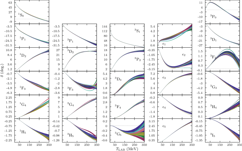
Figure 3: np phase-shifts in degrees for all partial waves with $J\leq 5$. The dark blue band represents the mean and standard deviation of thirteen different determinations of the NN interaction to their contemporary database Stoks et al. (1993, 1994); Wiringa et al. (1995); Machleidt (2001); Gross and Stadler (2008); Navarro Pérez et al. (2013b, a, 2014b, 2014c, 2014a). The red, green, olive green, light blue, light red and light green bands represent the statistical uncertainty of the DS-OPE Navarro Pérez et al. (2013b, a), DS-$\chi$TPE Navarro Pérez et al. (2014b, c), Gauss-OPE Navarro Pérez et al. (2014a), Gauss-$\chi$TPE, DS-$\Delta$BO and Gauss-$\Delta$BO potentials respectively.

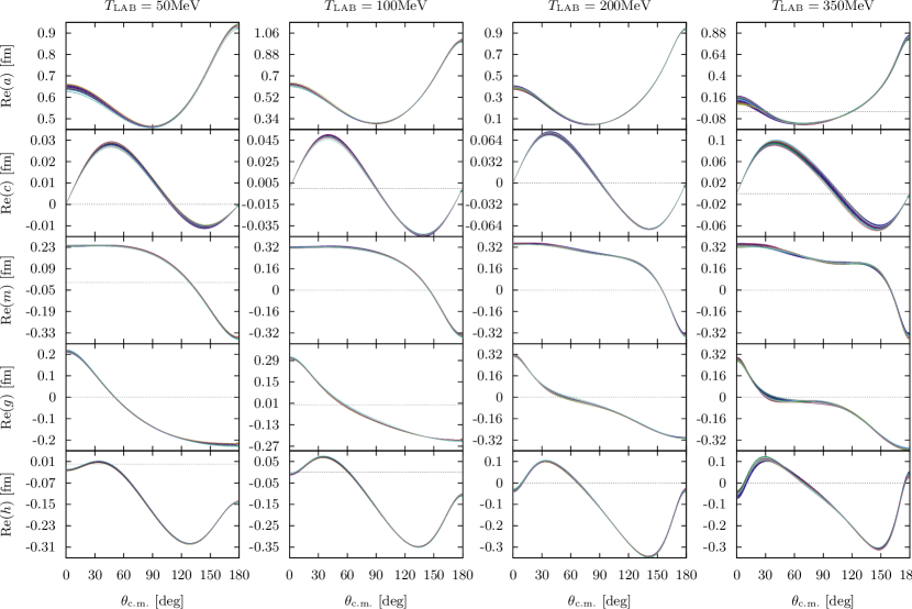
Figure 4: Same as Fig. 3 for the real part of the Wolfenstein parametrization of the np scattering amplitude in fm as a function of center of mass scattering angle at $T_{\rm LAB}=50,\ 100,\ 200,\ 350$MeV.

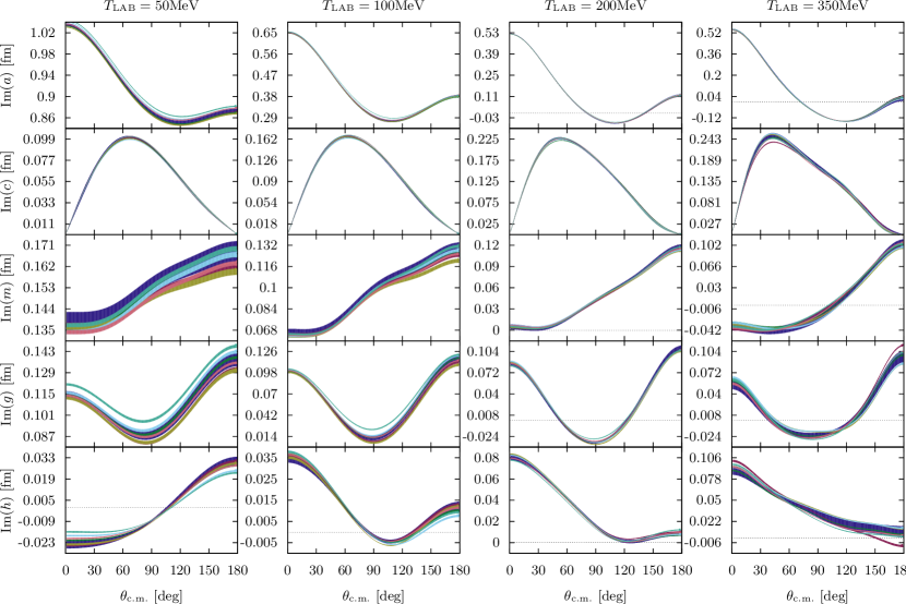
Figure 5: Same as Fig. 4 for the imaginary part.

Table 4: Averaged pp isovector phaseshifts in degrees (errors are systematic).

$E_{\rm LAB}$	${}^{1}S_{0}$	${}^{1}D_{2}$	${}^{1}G_{4}$	${}^{3}P_{0}$	${}^{3}P_{1}$	${}^{3}F_{3}$	${}^{3}P_{2}$	$\epsilon_{2}$	${}^{3}F_{2}$	${}^{3}F_{4}$	$\epsilon_{4}$	${}^{3}H_{4}$
1	$32.677$	$0.001$	$0.000$	$0.133$	$-0.079$	$-0.000$	$0.014$	$-0.001$	$0.000$	$0.000$	$-0.000$	$0.000$
	$\pm 0.016$	$\pm 0.000$	$\pm 0.000$	$\pm 0.000$	$\pm 0.001$	$\pm 0.000$	$\pm 0.000$	$\pm 0.000$	$\pm 0.000$	$\pm 0.000$	$\pm 0.000$	$\pm 0.000$
5	$54.895$	$0.042$	$0.000$	$1.575$	$-0.888$	$-0.004$	$0.214$	$-0.052$	$0.002$	$0.000$	$-0.000$	$0.000$
	$\pm 0.037$	$\pm 0.000$	$\pm 0.000$	$\pm 0.006$	$\pm 0.006$	$\pm 0.000$	$\pm 0.005$	$\pm 0.000$	$\pm 0.000$	$\pm 0.000$	$\pm 0.000$	$\pm 0.000$
10	$55.320$	$0.164$	$0.003$	$3.717$	$-2.028$	$-0.031$	$0.648$	$-0.200$	$0.013$	$0.001$	$-0.003$	$0.000$
	$\pm 0.065$	$\pm 0.000$	$\pm 0.000$	$\pm 0.017$	$\pm 0.015$	$\pm 0.000$	$\pm 0.012$	$\pm 0.001$	$\pm 0.000$	$\pm 0.000$	$\pm 0.000$	$\pm 0.000$
25	$48.848$	$0.689$	$0.040$	$8.552$	$-4.840$	$-0.231$	$2.479$	$-0.808$	$0.106$	$0.020$	$-0.049$	$0.004$
	$\pm 0.106$	$\pm 0.003$	$\pm 0.000$	$\pm 0.067$	$\pm 0.034$	$\pm 0.001$	$\pm 0.028$	$\pm 0.004$	$\pm 0.001$	$\pm 0.001$	$\pm 0.000$	$\pm 0.000$
50	$39.182$	$1.685$	$0.153$	$11.436$	$-8.161$	$-0.692$	$5.837$	$-1.707$	$0.345$	$0.108$	$-0.197$	$0.026$
	$\pm 0.115$	$\pm 0.017$	$\pm 0.001$	$\pm 0.169$	$\pm 0.044$	$\pm 0.008$	$\pm 0.039$	$\pm 0.015$	$\pm 0.010$	$\pm 0.006$	$\pm 0.000$	$\pm 0.000$
100	$25.357$	$3.750$	$0.423$	$9.324$	$-13.109$	$-1.530$	$11.027$	$-2.675$	$0.853$	$0.471$	$-0.549$	$0.111$
	$\pm 0.136$	$\pm 0.051$	$\pm 0.006$	$\pm 0.327$	$\pm 0.085$	$\pm 0.048$	$\pm 0.052$	$\pm 0.036$	$\pm 0.054$	$\pm 0.016$	$\pm 0.003$	$\pm 0.002$
150	$15.229$	$5.639$	$0.706$	$4.532$	$-17.379$	$-2.142$	$14.059$	$-2.954$	$1.271$	$1.011$	$-0.868$	$0.221$
	$\pm 0.231$	$\pm 0.047$	$\pm 0.004$	$\pm 0.383$	$\pm 0.135$	$\pm 0.135$	$\pm 0.062$	$\pm 0.032$	$\pm 0.117$	$\pm 0.020$	$\pm 0.008$	$\pm 0.011$
200	$7.076$	$7.212$	$1.005$	$-0.494$	$-21.273$	$-2.568$	$15.768$	$-2.914$	$1.499$	$1.628$	$-1.132$	$0.343$
	$\pm 0.281$	$\pm 0.087$	$\pm 0.014$	$\pm 0.313$	$\pm 0.252$	$\pm 0.265$	$\pm 0.118$	$\pm 0.041$	$\pm 0.183$	$\pm 0.037$	$\pm 0.012$	$\pm 0.028$
250	$0.212$	$8.487$	$1.311$	$-5.160$	$-24.784$	$-2.809$	$16.721$	$-2.724$	$1.457$	$2.220$	$-1.340$	$0.474$
	$\pm 0.264$	$\pm 0.107$	$\pm 0.041$	$\pm 0.147$	$\pm 0.527$	$\pm 0.377$	$\pm 0.203$	$\pm 0.131$	$\pm 0.230$	$\pm 0.054$	$\pm 0.026$	$\pm 0.053$
300	$-5.694$	$9.525$	$1.605$	$-9.287$	$-27.880$	$-2.814$	$17.208$	$-2.460$	$1.093$	$2.710$	$-1.501$	$0.615$
	$\pm 0.354$	$\pm 0.088$	$\pm 0.068$	$\pm 0.452$	$\pm 0.962$	$\pm 0.375$	$\pm 0.323$	$\pm 0.264$	$\pm 0.236$	$\pm 0.063$	$\pm 0.046$	$\pm 0.083$
350	$-10.828$	$10.375$	$1.865$	$-12.813$	$-30.527$	$-2.447$	$17.376$	$-2.157$	$0.389$	$3.048$	$-1.623$	$0.767$
	$\pm 0.747$	$\pm 0.347$	$\pm 0.084$	$\pm 1.091$	$\pm 1.565$	$\pm 0.412$	$\pm 0.553$	$\pm 0.446$	$\pm 0.233$	$\pm 0.079$	$\pm 0.063$	$\pm 0.120$

Table 5: Averaged np isovector phaseshifts in degrees (errors are systematic).

$E_{\rm LAB}$	${}^{1}S_{0}$	${}^{1}D_{2}$	${}^{1}G_{4}$	${}^{3}P_{0}$	${}^{3}P_{1}$	${}^{3}F_{3}$	${}^{3}P_{2}$	$\epsilon_{2}$	${}^{3}F_{2}$	${}^{3}F_{4}$	$\epsilon_{4}$	${}^{3}H_{4}$
1	$62.105$	$0.001$	$0.000$	$0.178$	$-0.106$	$-0.000$	$0.022$	$-0.001$	$0.000$	$0.000$	$-0.000$	$0.000$
	$\pm 0.039$	$\pm 0.000$	$\pm 0.000$	$\pm 0.002$	$\pm 0.001$	$\pm 0.000$	$\pm 0.000$	$\pm 0.000$	$\pm 0.000$	$\pm 0.000$	$\pm 0.000$	$\pm 0.000$
5	$63.689$	$0.041$	$0.000$	$1.626$	$-0.923$	$-0.004$	$0.255$	$-0.048$	$0.002$	$0.000$	$-0.000$	$0.000$
	$\pm 0.079$	$\pm 0.000$	$\pm 0.000$	$\pm 0.024$	$\pm 0.011$	$\pm 0.000$	$\pm 0.004$	$\pm 0.000$	$\pm 0.000$	$\pm 0.000$	$\pm 0.000$	$\pm 0.000$
10	$60.038$	$0.155$	$0.002$	$3.672$	$-2.032$	$-0.026$	$0.718$	$-0.183$	$0.011$	$0.001$	$-0.003$	$0.000$
	$\pm 0.114$	$\pm 0.001$	$\pm 0.000$	$\pm 0.064$	$\pm 0.027$	$\pm 0.000$	$\pm 0.011$	$\pm 0.001$	$\pm 0.000$	$\pm 0.000$	$\pm 0.000$	$\pm 0.000$
25	$51.011$	$0.670$	$0.032$	$8.250$	$-4.801$	$-0.199$	$2.595$	$-0.753$	$0.091$	$0.017$	$-0.039$	$0.003$
	$\pm 0.189$	$\pm 0.002$	$\pm 0.000$	$\pm 0.201$	$\pm 0.069$	$\pm 0.001$	$\pm 0.029$	$\pm 0.009$	$\pm 0.001$	$\pm 0.001$	$\pm 0.000$	$\pm 0.000$
50	$40.644$	$1.686$	$0.134$	$10.955$	$-8.151$	$-0.620$	$5.970$	$-1.635$	$0.310$	$0.098$	$-0.169$	$0.021$
	$\pm 0.324$	$\pm 0.013$	$\pm 0.002$	$\pm 0.361$	$\pm 0.114$	$\pm 0.008$	$\pm 0.056$	$\pm 0.033$	$\pm 0.010$	$\pm 0.006$	$\pm 0.001$	$\pm 0.000$
100	$26.772$	$3.797$	$0.390$	$8.752$	$-13.218$	$-1.421$	$11.118$	$-2.633$	$0.795$	$0.447$	$-0.499$	$0.094$
	$\pm 0.620$	$\pm 0.044$	$\pm 0.018$	$\pm 0.479$	$\pm 0.184$	$\pm 0.046$	$\pm 0.086$	$\pm 0.071$	$\pm 0.051$	$\pm 0.013$	$\pm 0.005$	$\pm 0.002$
150	$16.791$	$5.699$	$0.660$	$3.937$	$-17.582$	$-2.028$	$14.086$	$-2.950$	$1.198$	$0.978$	$-0.812$	$0.195$
	$\pm 0.770$	$\pm 0.078$	$\pm 0.047$	$\pm 0.475$	$\pm 0.239$	$\pm 0.129$	$\pm 0.085$	$\pm 0.065$	$\pm 0.112$	$\pm 0.019$	$\pm 0.014$	$\pm 0.011$
200	$8.759$	$7.262$	$0.945$	$-1.095$	$-21.541$	$-2.462$	$15.736$	$-2.937$	$1.411$	$1.586$	$-1.079$	$0.310$
	$\pm 0.736$	$\pm 0.125$	$\pm 0.079$	$\pm 0.359$	$\pm 0.319$	$\pm 0.257$	$\pm 0.114$	$\pm 0.045$	$\pm 0.180$	$\pm 0.046$	$\pm 0.025$	$\pm 0.027$
250	$1.982$	$8.516$	$1.248$	$-5.757$	$-25.099$	$-2.713$	$16.638$	$-2.764$	$1.350$	$2.170$	$-1.295$	$0.436$
	$\pm 0.561$	$\pm 0.126$	$\pm 0.105$	$\pm 0.135$	$\pm 0.547$	$\pm 0.359$	$\pm 0.190$	$\pm 0.134$	$\pm 0.230$	$\pm 0.077$	$\pm 0.040$	$\pm 0.051$
300	$-3.855$	$9.529$	$1.564$	$-9.874$	$-28.229$	$-2.716$	$17.082$	$-2.511$	$0.965$	$2.649$	$-1.465$	$0.573$
	$\pm 0.357$	$\pm 0.128$	$\pm 0.121$	$\pm 0.430$	$\pm 0.958$	$\pm 0.329$	$\pm 0.329$	$\pm 0.283$	$\pm 0.231$	$\pm 0.097$	$\pm 0.059$	$\pm 0.081$
350	$-8.923$	$10.352$	$1.880$	$-13.387$	$-30.902$	$-2.307$	$17.213$	$-2.217$	$0.239$	$2.975$	$-1.597$	$0.721$
	$\pm 0.533$	$\pm 0.416$	$\pm 0.140$	$\pm 1.081$	$\pm 1.547$	$\pm 0.478$	$\pm 0.587$	$\pm 0.481$	$\pm 0.208$	$\pm 0.102$	$\pm 0.079$	$\pm 0.120$

Table 6: Averaged np isoscalar phaseshifts in degrees (errors are systematic).

$E_{\rm LAB}$	${}^{1}P_{1}$	${}^{1}F_{3}$	${}^{3}D_{2}$	${}^{3}G_{4}$	${}^{3}S_{1}$	$\epsilon_{1}$	${}^{3}D_{1}$	${}^{3}D_{3}$	$\epsilon_{3}$	${}^{3}G_{3}$
1	$-0.188$	$-0.000$	$0.006$	$0.000$	$147.748$	$0.102$	$-0.005$	$0.000$	$0.000$	$-0.000$
	$\pm 0.002$	$\pm 0.000$	$\pm 0.000$	$\pm 0.000$	$\pm 0.093$	$\pm 0.001$	$\pm 0.000$	$\pm 0.000$	$\pm 0.000$	$\pm 0.000$
5	$-1.513$	$-0.010$	$0.218$	$0.001$	$118.169$	$0.637$	$-0.178$	$0.002$	$0.012$	$-0.000$
	$\pm 0.018$	$\pm 0.000$	$\pm 0.001$	$\pm 0.000$	$\pm 0.213$	$\pm 0.012$	$\pm 0.001$	$\pm 0.000$	$\pm 0.000$	$\pm 0.000$
10	$-3.110$	$-0.064$	$0.842$	$0.012$	$102.587$	$1.079$	$-0.665$	$0.005$	$0.080$	$-0.003$
	$\pm 0.045$	$\pm 0.000$	$\pm 0.003$	$\pm 0.000$	$\pm 0.300$	$\pm 0.029$	$\pm 0.003$	$\pm 0.001$	$\pm 0.000$	$\pm 0.000$
25	$-6.498$	$-0.421$	$3.689$	$0.170$	$80.559$	$1.611$	$-2.757$	$0.037$	$0.553$	$-0.053$
	$\pm 0.135$	$\pm 0.001$	$\pm 0.024$	$\pm 0.000$	$\pm 0.447$	$\pm 0.087$	$\pm 0.017$	$\pm 0.011$	$\pm 0.000$	$\pm 0.000$
50	$-9.905$	$-1.142$	$8.896$	$0.724$	$62.645$	$1.823$	$-6.351$	$0.285$	$1.614$	$-0.263$
	$\pm 0.243$	$\pm 0.004$	$\pm 0.109$	$\pm 0.002$	$\pm 0.538$	$\pm 0.182$	$\pm 0.044$	$\pm 0.050$	$\pm 0.004$	$\pm 0.001$
100	$-14.416$	$-2.291$	$17.091$	$2.204$	$43.088$	$2.096$	$-12.110$	$1.358$	$3.502$	$-0.978$
	$\pm 0.256$	$\pm 0.022$	$\pm 0.311$	$\pm 0.023$	$\pm 0.512$	$\pm 0.328$	$\pm 0.080$	$\pm 0.141$	$\pm 0.031$	$\pm 0.012$
150	$-18.046$	$-3.100$	$21.860$	$3.737$	$30.644$	$2.538$	$-16.358$	$2.590$	$4.835$	$-1.871$
	$\pm 0.188$	$\pm 0.057$	$\pm 0.383$	$\pm 0.079$	$\pm 0.428$	$\pm 0.377$	$\pm 0.081$	$\pm 0.165$	$\pm 0.067$	$\pm 0.032$
200	$-21.189$	$-3.751$	$24.196$	$5.191$	$21.244$	$3.107$	$-19.658$	$3.569$	$5.730$	$-2.803$
	$\pm 0.218$	$\pm 0.119$	$\pm 0.315$	$\pm 0.146$	$\pm 0.392$	$\pm 0.338$	$\pm 0.074$	$\pm 0.163$	$\pm 0.079$	$\pm 0.053$
250	$-23.885$	$-4.344$	$25.104$	$6.515$	$13.551$	$3.749$	$-22.330$	$4.194$	$6.324$	$-3.706$
	$\pm 0.328$	$\pm 0.189$	$\pm 0.157$	$\pm 0.186$	$\pm 0.474$	$\pm 0.255$	$\pm 0.137$	$\pm 0.193$	$\pm 0.073$	$\pm 0.075$
300	$-26.143$	$-4.920$	$25.273$	$7.673$	$6.966$	$4.418$	$-24.544$	$4.507$	$6.714$	$-4.552$
	$\pm 0.457$	$\pm 0.226$	$\pm 0.302$	$\pm 0.194$	$\pm 0.695$	$\pm 0.220$	$\pm 0.263$	$\pm 0.212$	$\pm 0.118$	$\pm 0.113$
350	$-27.966$	$-5.487$	$25.121$	$8.631$	$1.176$	$5.069$	$-26.380$	$4.593$	$6.963$	$-5.336$
	$\pm 0.565$	$\pm 0.212$	$\pm 0.838$	$\pm 0.242$	$\pm 1.017$	$\pm 0.381$	$\pm 0.506$	$\pm 0.270$	$\pm 0.195$	$\pm 0.179$

To estimate the systematic uncertainties of the NN interaction at low energies we take different realistic potentials and compare their low energy threshold parameters. Any estimate of the systematic errors based on variations of the potential form or possible radial dependences will provide a lower bound to the uncertainties. Besides the form of the potential used to fit the data, another source of systematic error is the selection of the data itself, due to addition of possible future data. Thus, the changes from the $3\sigma$-selected database of the Nijmegen analysis 20 years ago comprising $N=4301$ np and pp scattering data Stoks et al. (1993) to our recent $3\sigma$-self-consistent database Navarro Pérez et al. (2013b, a) with about $N=6713$ np and pp scattering data can be taken as an estimate on how much do we expect our predictions to change when a large body of new data is incorporated.

Here we consider nine realistic local or minimally non-local potentials (i.e. containing $L^{2}$ dependences or quadratic tensor interactions) such as NijmII Stoks et al. (1994), Reid93 Stoks et al. (1994), AV18 Wiringa et al. (1995), which provided a $\chi^{2}/{\rm d.o.f}\sim 1$ to the Nijmegen database Stoks et al. (1993), and the new DS-OPE Navarro Pérez et al. (2013b, a), DS-$\chi$TPE Navarro Pérez et al. (2014b, c), Gauss-OPE Navarro Pérez et al. (2014a), Gauss-$\chi$TPE, DS-$\Delta$BO and Gauss-$\Delta$BO which also provide a $\chi^{2}/{\rm d.o.f}\sim 1$ to the Granada database Navarro Pérez et al. (2013a). To stress the obvious, we associate the increase of about 2400 np and pp data from the Nijmegen to the Granada databases with an additional systematic error, foreseeing the possible impact that additional new data might have in the future . The values of low energy parameters for the NijmII Stoks et al. (1994), Reid93 Stoks et al. (1994) have been determined already Pavon Valderrama and Ruiz Arriola (2005) but numerical precision has been improved in the present work; the values for the remaining potentials are also determined here. Our results are presented in Table 3 (second line of each partial wave) which shows the mean and standard deviation of the low energy threshold parameters for the nine local potentials. Comparison of the errors quoted in Table 3 clearly shows that the main uncertainty in the low energy parameters is due to the different representations or choices of high-quality potentials and not to the propagation of experimental uncertainties used to fix the most-likely potential chosen for the least squares $\chi^{2}$-analysis.

Our conclusions on systematic uncertainties at low energies are vividly illustrated in Fig. 2. As we see the spread of all potential results is larger than the statistical error band, which is our main point. In Figures 6 and 7 we show our three local interactions Gauss-OPE Navarro Pérez et al. (2014a), Gauss-$\chi$TPE and Gauss-$\Delta$BO in comparison with the AV18 Wiringa et al. (1995), Reid93 Stoks et al. (1994) and NijmII Stoks et al. (1994) potentials as a function of $r$. Again, it can clearly be seen that the spread of the different interactions, which acounts for the systematic uncertainty, is significantly larger than the statistical uncertainty inferred in the potentials from the experimental errors of the scattering data. Notice however the different scale used on the $y$-axis of every pannel. This may make the discrepancies appear to be about the same order in all channels, which is not the case. Still, the systematic spread is always larger than the statistical error bands. An interpretation of the scattering data and evaluation of the Skyrme coefficients or equivalent counterterms in different partial waves was proposed in our previous works Navarro Pérez et al. (2013d, 2015a) with a focus on their scale dependence and statistical uncertainties . The trend observed in all physical observables in this paper confirms also the findings in Ref. Navarro Pérez et al. (2016a) regarding the systematic uncertainties.

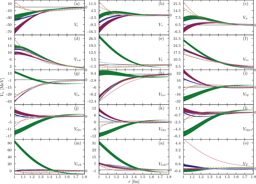
Figure 6: Potentials in different channels in configuration space for short distances $1<r<1.8$fm. The blue, red and green bands represent the Gauss-OPE Navarro Pérez et al. (2014a), Gauss-$\chi$TPE and Gauss-$\Delta$BO potentials respectively with their statistical uncertainty. For comparison we also show the local potentials AV18 Wiringa et al. (1995) (dot-dashed olive green line), Reid93 Stoks et al. (1994) (dotted light blue line) and NijmII Stoks et al. (1994) (dashed light red line).

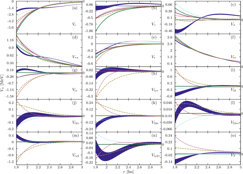
Figure 7: Same as Fig.6 for the intermediate range $1.8<r<3$fm.

This analysis is sufficient to prove that the lower bound on the systematic error is at least one order of magnitude larger than the statistical errors. Our results show that this conclusion is valid for all the scattering properties, such as low energy parameters, phase-shifts and amplitudes.

VI On the portability of the partial wave analysis

One problem we want to address has to do with the portability of our analysis and by extension of any PWA. One of the main technical problems in carrying out a PWA in NN scattering is the inclusion of many effects which are crucial to provide a convincing and statistically sound fit to experimental data. Among them, the inclusion of the long-range magnetic dipole local and anysotropic interations needs summing up about 1000 partial waves and coordinate space methods are strongly preferred over the momentum space approaches, where implementation of these indispensable effects is a real challenge still unsolved.

When this project was started the idea was to provide the most relevant and portable information. Traditionally it has been thought that phase-shifts with their corresponding covariance matrices obtained from the fit represent the inherent uncertainty of the interaction. Our experience does not support this view, and statistically good fits to some phases at arbitrary energies do not provide statistically good fits to scattering data, most often very bad ones Navarro Pérez et al. (2015b). Another possibility which turns out to provide a better approximation to our fit to data can be found by fitting the Wolfenstein parameters within the systematic spread found from the different potentials. This obviously incorporates the correlations among the different phase shifts, but even if $\chi^{2}/\nu\sim 1$ to the Wolfenstein parameters we typically find $\chi^{2}/\nu\sim 4$ to the data.

However, in view of the results of the present paper where the form of the potential itself representing the interaction provides the largest uncertainty, we think that our results are best represented by an average over the 6 potentials analyzed here. For the lower phases this is summarized in Tables 4, 5 and 6 and complete tables can be provided upon request. As said, the corresponding errors are comparable with the spread found using the previous PWA carried out in the past.

VII Conclusions and Outlook

We summarize our results. In the present paper we have confronted statistical vs systematic errors in the description of a largest body of NN scattering below LAB energy $350{\rm MeV}$ to date, namely $6713$ np and pp scattering data collected from 1950 till 2013. We use the classical statistical rules to evaluate the corresponding uncertainties of the inferred potential, after the self-consistency of the fit has been confidently established via checking Tail-Sensitive normality tests Navarro Pérez et al. (2015a). We approach the determination of systematic uncertainties by using 6 model potentials which describe the same database comprising 6713 NN scattering data in a statistically significant way. Thus, we have calculated and compared phases and scattering amplitudes with their statistical uncertainties. We have also calculated the low energy threshold parameters of the coupled channel effective range expansion for all partial waves with $j\leq 5$ by using a discrete version of the variable S-matrix method. This approach provides satisfactory numerical precision at a low computational cost, qualifying as a suitable method to compare statistical vs systematic errors. Statistical uncertainties are propagated via the bootstrap method Navarro Pérez et al. (2014d) where a family of DS-OPE potential parameters is fitted after experimental data are replicated. We also made a first estimate of the systematic uncertainties of the NN interaction by taking nine different realistic potentials (i.e. with $\chi^{2}/{\rm d.o.f}\lesssim 1$) and calculating the low energy threshold parameters with each of them. These estimates should be taken as a lower bound on the systematic uncertainties. In accordance with preliminary estimates Navarro Pérez et al. (2012a, b), the systematic uncertainties tend to be at least an order of magnitude larger than the statistical ones. The same trend between statistical and systematic uncertainties is found when comparing phaseshifts and scattering amplitudes. The present results encode the full PWA at low energies and have a direct impact in ab initio nuclear structure calculations in nuclear physics. The low energy threshold parameters could also be used as a starting point to the determination and error propagation of low energy interactions with the proper long distance behavior in addition to the universal One Pion Exchange interaction.

Recently, there have been impressive bench-marking estimates on uncertainties based on chiral NN and NNN forces in an order by order scheme for light nuclei with $A\leq 16$ Carlsson et al. (2015). Such estimates are much larger than our simple preliminary estimates of 0.5 MeV in the binding energy per nucleon Navarro Pérez et al. (2012a, b). The upgrade of our results incorporating the present systematic errors would increase our estimate by a factor of four Navarro Pérez et al. (2016a). The interactions we have designed in this paper have the important property of being statistically equivalent for a large NN database, and thus they can be used to carry out comprehensive studies regarding different aspects of binding in finite nuclei and in particular the impact on the predictive power of nuclear structure and nuclear reactions calculations which are now underway for the lighest $A=3,4$ systems and will be analyzed in the future.

Appendix A Model potentials

We provide here details on the model potentials not described previously.

A.1 The Gauss-$\chi$TPE Potential

On this appendix we present the details of the Gaussian-$\chi$TPE potential introduced on this article. The structure of the potential is very similar to the Gaussian-OPE potential presented in Navarro Pérez et al. (2014a). The interaction is decomposed as

$$V(\vec{r})=V_{\rm short}(r)\theta(r_{c}-r)+V_{\rm long}(r)\theta(r-r_{c}),$$ (8)

where the short component is written as

$$V_{\rm short}(\vec{r})=\sum_{n=1}^{21}\hat{O}_{n}\left[\sum_{i=1}^{N}V_{i,n}F_{i}(r)\right]$$ (9)

where $\hat{O}_{n}$ are the set of operators in the extended AV18 basis Wiringa et al. (1995); Navarro Pérez et al. (2012a, b), $V_{i,n}$ are unknown coefficients to be determined from data and $F_{i}(r)=e^{-r^{2}/(2a_{i}^{2})}$ where $a_{i}=a/(1+i)$. $V_{\rm long}(\vec{r})$ contains a Charge-Dependent (CD) One pion exchange (OPE) (with a common $f^{2}=0.075$ Navarro Pérez et al. (2012a, b)), a charge independent chiral two pion exchange ($\chi$-TPE) tail and electromagnetic (EM) corrections which are kept fixed throughout. This corresponds to

$$V_{\rm long}(\vec{r})=V_{\rm OPE}(\vec{r})+V_{\chi\rm TPE}(\vec{r})+V_{\rm em}(\vec{r})\,.$$ (10)

The boundary between the phenomenological $V_{\rm short}(r)$ and the fixed $V_{\rm long}$ part $r_{c}$ is fixed at $1.8$fm. The parameter $a$, that determines the width of each gaussian function was used as an aditional fitting parameter obtaining the value $1.4335\pm 0.0302$ fm. Table 7 shows the values, with statistical uncertainties, of the $V_{i,n}$ coefficients. Like in all our previous potential analyses, although the form of the complete potential is expressed in the operator basis the statistical analysis is carried out more effectively in terms of some low and independent partial waves contributions to the potential from which all other higher partial waves are consistently deduced (see Ref. Navarro Pérez et al. (2013b, a)). For the chiral constants determining $\chi$-TPE part we used the values obtained on Navarro Pérez et al. (2014b) from fitting to the self-consistent NN database, namely $c_{1}=-0.41523$, $c_{3}=-4.66076$ and $c_{4}=4.31725$ GeV^-1. The resulting potential yields a merit figure of $\chi^{2}/{\rm d.o.f.}=1.09$ and the residuals tested positively for a standard normal distribution after rescaling by the birge factor (see Ref. Navarro Pérez et al. (2014a) and appendix B here).

Table 7: Operator coefficients $V_{i,n}$ (in MeV) with their errors for the Gauss-$\chi$TPE, DS-$\Delta$BO and Gauss-$\Delta$BO potentials. The coefficients of the $tT$, $\tau z$ and $\sigma\tau z$ operators are set to zero

	Gauss-$\chi$TPE			DS-$\Delta$BO			Gauss-$\Delta$BO
$\hat{O}_{n}$	$V_{1}$	$V_{2}$	$V_{3}$	$V_{1}$	$V_{2}$	$V_{3}$	$V_{1}$	$V_{2}$	$V_{3}$
$c$	$9.6837$	$-825.0435$	$945.4663$	$21.2098$	$4.2506$	$-2.3108$	$-7.3514$	$-157.2374$	$82.0322$
	$\pm 5.9084$	$\pm 97.9106$	$\pm 43.7258$	$\pm 0.7545$	$\pm 0.4744$	$\pm 0.1302$	$\pm 2.9646$	$\pm 18.8009$	$\pm 23.5960$
$\tau$	$12.7705$	$-123.1648$	$-316.2405$	$-12.2427$	$-4.2044$	$0.7355$	$-17.2568$	$173.3607$	$-502.4170$
	$\pm 4.1353$	$\pm 51.3913$	$\pm 37.9668$	$\pm 0.3630$	$\pm 0.2142$	$\pm 0.0460$	$\pm 2.2635$	$\pm 13.1983$	$\pm 29.6577$
$\sigma$	$18.5052$	$-33.2765$	$-421.9382$	$-25.8805$	$11.4536$	$-0.2993$	$-14.0544$	$211.4154$	$-524.6394$
	$\pm 3.9747$	$\pm 37.6690$	$\pm 42.1474$	$\pm 0.4332$	$\pm 0.1875$	$\pm 0.0350$	$\pm 2.7246$	$\pm 10.9153$	$\pm 19.4042$
$\tau\sigma$	$24.6014$	$66.2296$	$-351.1114$	$-15.0644$	$9.4391$	$0.4022$	$-0.5228$	$167.3510$	$-351.4668$
	$\pm 4.3676$	$\pm 19.7870$	$\pm 16.5232$	$\pm 0.1447$	$\pm 0.1341$	$\pm 0.0150$	$\pm 2.5883$	$\pm 6.1739$	$\pm 12.4842$
$t$	$4.2686$	$-23.5189$	$19.2503$	$0.0000$	$4.1612$	$-0.1994$	$-44.6418$	$340.6416$	$-295.9998$
	$\pm 1.1084$	$\pm 10.5193$	$\pm 9.5377$	$\pm 0.0000$	$\pm 0.1591$	$\pm 0.0298$	$\pm 1.2178$	$\pm 18.4712$	$\pm 17.8500$
$t\tau$	$51.9125$	$23.5189$	$-75.4314$	$0.0000$	$21.2745$	$0.5108$	$0.8113$	$209.6308$	$-210.4421$
	$\pm 5.7086$	$\pm 10.5193$	$\pm 5.3862$	$\pm 0.0000$	$\pm 0.0938$	$\pm 0.0226$	$\pm 2.4346$	$\pm 4.9184$	$\pm 6.2049$
$ls$	$2.9027$	$-401.1252$	$-33.0241$	$-22.4843$	$-14.0920$	$-1.1591$	$-93.5595$	$434.2099$	$-431.8457$
	$\pm 4.9308$	$\pm 20.0357$	$\pm 5.9716$	$\pm 0.6346$	$\pm 0.3326$	$\pm 0.0545$	$\pm 3.8004$	$\pm 29.5342$	$\pm 21.2608$
$ls\tau$	$-3.7375$	$-76.3035$	$-34.3932$	$-7.4948$	$-4.0634$	$-0.2078$	$-17.1960$	$94.0333$	$-175.8844$
	$\pm 2.3106$	$\pm 11.3094$	$\pm 1.0782$	$\pm 0.2115$	$\pm 0.1696$	$\pm 0.0348$	$\pm 1.1839$	$\pm 6.9873$	$\pm 7.0953$
$l2$	$-42.8284$	$494.8237$	$-97.5866$	$-3.1602$	$-7.4527$	$0.9505$	$73.0678$	$-506.6174$	$661.2658$
	$\pm 2.6104$	$\pm 56.7825$	$\pm 7.6448$	$\pm 0.1346$	$\pm 0.2228$	$\pm 0.0459$	$\pm 1.0393$	$\pm 16.7099$	$\pm 34.9700$
$l2\tau$	$-6.9591$	$45.6004$	$96.0890$	$2.1654$	$-5.7220$	$0.3142$	$29.7916$	$-242.6322$	$340.6513$
	$\pm 1.2133$	$\pm 14.9971$	$\pm 6.7830$	$\pm 0.0623$	$\pm 0.0995$	$\pm 0.0172$	$\pm 0.8288$	$\pm 5.9885$	$\pm 15.0560$
$l2\sigma$	$-15.0107$	$128.9282$	$90.3201$	$4.4383$	$-4.1874$	$0.3270$	$27.8688$	$-214.1951$	$312.4192$
	$\pm 1.1788$	$\pm 19.0121$	$\pm 9.1420$	$\pm 0.0730$	$\pm 0.0878$	$\pm 0.0147$	$\pm 0.6741$	$\pm 5.0498$	$\pm 13.3164$
$l2\sigma\tau$	$-2.3215$	$0.9704$	$72.9793$	$2.5524$	$-1.7972$	$0.1081$	$11.5384$	$-97.7867$	$144.2162$
	$\pm 0.5389$	$\pm 5.2064$	$\pm 3.0161$	$\pm 0.0243$	$\pm 0.0487$	$\pm 0.0054$	$\pm 0.4459$	$\pm 1.6616$	$\pm 5.5114$
$ls2$	$18.1617$	$-59.9055$	$-66.0483$	$-7.4948$	$20.8558$	$-1.4306$	$-140.3961$	$1021.2501$	$-863.6915$
	$\pm 1.8609$	$\pm 21.5240$	$\pm 11.9432$	$\pm 0.2115$	$\pm 0.3172$	$\pm 0.0509$	$\pm 2.5246$	$\pm 49.6812$	$\pm 42.5216$
$ls2\tau$	$-2.3108$	$88.2359$	$-68.7865$	$-2.4983$	$9.5656$	$-0.5098$	$-46.6431$	$375.7827$	$-351.7689$
	$\pm 0.9193$	$\pm 13.2382$	$\pm 2.1564$	$\pm 0.0705$	$\pm 0.1231$	$\pm 0.0229$	$\pm 1.1847$	$\pm 14.0073$	$\pm 14.1905$
$T$	$0.4092$	$-6.9622$	$19.9535$	$0.8070$	$0.0731$	$-0.0759$	$1.8127$	$-13.8327$	$25.1923$
	$\pm 1.0118$	$\pm 8.6713$	$\pm 16.1725$	$\pm 0.2166$	$\pm 0.0401$	$\pm 0.0159$	$\pm 0.7598$	$\pm 4.9259$	$\pm 7.6163$
$\sigma T$	$-0.4092$	$6.9622$	$-19.9535$	$-0.8070$	$-0.0731$	$0.0759$	$-1.8127$	$13.8327$	$-25.1923$
	$\pm 1.0118$	$\pm 8.6713$	$\pm 16.1725$	$\pm 0.2166$	$\pm 0.0401$	$\pm 0.0159$	$\pm 0.7598$	$\pm 4.9259$	$\pm 7.6163$
$l2T$	$-0.0682$	$1.1604$	$-3.3256$	$-0.1345$	$-0.0122$	$0.0126$	$-0.3021$	$2.3055$	$-4.1987$
	$\pm 0.1686$	$\pm 1.4452$	$\pm 2.6954$	$\pm 0.0361$	$\pm 0.0067$	$\pm 0.0027$	$\pm 0.1266$	$\pm 0.8210$	$\pm 1.2694$
$l2\sigma T$	$0.0682$	$-1.1604$	$3.3256$	$0.1345$	$0.0122$	$-0.0126$	$0.3021$	$-2.3055$	$4.1987$
	$\pm 0.1686$	$\pm 1.4452$	$\pm 2.6954$	$\pm 0.0361$	$\pm 0.0067$	$\pm 0.0027$	$\pm 0.1266$	$\pm 0.8210$	$\pm 1.2694$

A.2 The $\Delta$ Born-Oppenheimer potential

Here we will detail the Born-Oppenheimer potential with $\Delta$ terms fitted to the Granada self-consistent database and introduced in this work as a new source of systematic uncertainty of the NN interaction (see e.g. Ruiz Arriola and Calle Cordon (2009); Cordon and Ruiz Arriola (2011) for some details). In general this potential has the same form of Eq.(8) with a clear boundary between the short range phenomelogical part and the long-range pion-exchange tail; in particular the long range part features squared Yukawa contributions that result from including an intermediate $\Delta$ excitation.

The introduction of the $\Delta$-isobar as a dynamical degree of freedom in the elastic NN channel requires extra terms on the Lipmann-Schwinger equation. Applying the Born-Oppenheimer approximation to second order results in more complicated structures than just OPE and also a contribution to the central channel. This additional terms are all proportional to $e^{-2m_{\pi}r}$ in a TPE-like fashion. The approximation can be expressed as

$$\bar{V}_{NN,NN}^{1\pi+2\pi+\dots}({\bm{r}}) = V_{NN,NN}^{1\pi}({\bm{r}})-2\frac{|V_{NN,N\Delta}^{1\pi}({\bm{r}})|^{2}}{\Delta}$$ (11)

$$- \frac{1}{2}\frac{|V_{NN,\Delta\Delta}^{1\pi}({\bm{r}})|^{2}}{\Delta}+\mathcal{O}(V^{3}),$$

where $\Delta\equiv M_{\Delta}-M_{N}=293$MeV and the transition potentials are given by

$$V_{AB,CD}({\bm{r}}) = (\bm{\tau}_{AB}\cdot{\bm{\tau}}_{CD})\left\{{\bm{\sigma}}_{AB}\cdot{\bm{\sigma}}_{CD}\left[W_{S}^{1\pi}(r)\right]_{AB,CD}\right.$$ (12)

$$+ \left.\left[S_{12}\right]_{AB,CD}\left[W_{T}^{1\pi}(r)\right]_{AB,CD}\right\},$$

being $W_{S}^{1\pi}(r)$ and $W_{T}^{1\pi}(r)$ the usual spin-spin and isovector tensor components of the one OPE potential.

After dealing with the squared transitions of Eq.(11) and excluding the OPE part, the $\Delta$ Born-Oppenheimer potential can be written as

$$V_{\Delta\rm BO}({\bm{r}}) = [V_{C}(r)+V_{S}(r){\bm{\sigma}}_{1}\cdot{\bm{\sigma}}_{2}+V_{T}(r)]$$

$$+ [W_{C}(r)+W_{S}(r){\bm{\sigma}}_{1}\cdot{\bm{\sigma}}_{2}+W_{T}(r)]{\bm{\tau}}_{1}\cdot{\bm{\tau}}_{2},$$

with components

$$V_{C}(r) = -\frac{8f_{\pi N\Delta}^{2}(f_{\pi N\Delta}^{2}+9f_{\pi NN}^{2})m_{\pi}^{2}}{81\Delta}[2Y_{2}(m_{\pi}r)^{2}+Y_{0}(m_{\pi}r)^{2}],$$

$$V_{S}(r) = -\frac{4f_{\pi N\Delta}^{2}(f_{\pi N\Delta}^{2}-18f_{\pi NN}^{2})m_{\pi}^{2}}{243\Delta}[Y_{2}(m_{\pi}r)^{2}-Y_{0}(m_{\pi}r)^{2}],$$

$$V_{T}(r) = \frac{4f_{\pi N\Delta}^{2}(f_{\pi N\Delta}^{2}-18f_{\pi NN}^{2})m_{\pi}^{2}}{243\Delta}[Y_{2}(m_{\pi}r)^{2}-Y_{0}(m_{\pi}r)Y_{2}(m_{\pi}r)],$$

$$W_{C}(r) = \frac{4f_{\pi N\Delta}^{2}(f_{\pi N\Delta}^{2}-18f_{\pi NN}^{2})m_{\pi}^{2}}{243\Delta}[2Y_{2}(m_{\pi}r)^{2}+Y_{0}(m_{\pi}r)^{2}],$$

$$W_{S}(r) = +\frac{2f_{\pi N\Delta}^{2}(f_{\pi N\Delta}^{2}+36f_{\pi NN}^{2})m_{\pi}^{2}}{729\Delta}[Y_{2}(m_{\pi}r)^{2}-Y_{0}(m_{\pi}r)^{2}],$$

$$W_{T}(r) = -\frac{2f_{\pi N\Delta}^{2}(f_{\pi N\Delta}^{2}+36f_{\pi NN}^{2})m_{\pi}^{2}}{729\Delta}[Y_{2}(m_{\pi}r)^{2}-Y_{0}(m_{\pi}r)Y_{2}(m_{\pi}r)],$$ (14)

where $Y_{0}(x)=e^{-x}/x$ and $Y_{2}(x)=Y_{0}(x)(1+3/x+3/x^{2})$. With this form the coupling $f_{\pi N\Delta}$ can be determined by fitting to NN data. The long range part is explicitly given by

$$V_{\rm long}(\vec{r})=V_{\rm OPE}(\vec{r})+V_{\Delta\rm BO}(\vec{r})+V_{\rm em}(\vec{r})\,.$$ (15)

Note that we include the long range electromagnetic effects in the interaction and fits, but we only give the nuclear part of the phase-shifts. See Navarro Pérez et al. (2013a) for details on how we deal with the electromagnetic interaction.

For the short range part given in Eq.(9) we implement two choices for the radial functions. The first one is a Delta-Shell representation $F_{i}(r)=\Delta r\delta(r-r_{i})$ with $\Delta r=r_{i+1}-r_{i}=0.6$fm and the second one is the guassian functions given in the previous section. In both cases the cut radius is set to $r_{c}=1.8$fm. An initial fit was made to the Granada self-consistent data base with the DS representation for the short range part and including the $f_{\pi N\Delta}$ coupling as a fitting parameter. A merit figure of $\chi^{2}/{\rm d.o.f.}=1.12$ is obtained. The potential parameters in the operator basis are given in table 7; the fit gives a coupling of $f_{\pi N\Delta}=(2.1778\pm 0.0143)f_{\pi NN}$. A second fit uses the SOG representation and the same fixed value of the $N\Delta$ coupling obtained with the previous fit. For this case the merit figure is $\chi^{2}/{\rm d.o.f.}=1.14$. The Potential parameters are also given in table 7

Appendix B Normality of residuals

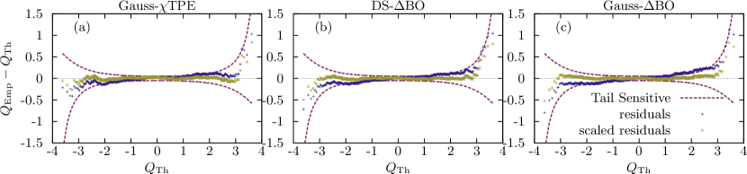
Figure 8: Rotated Quantile-Quantile plot for the residuals (blue crosses) and scaled residuals (yellow diagonal crosses) of the three new phenomenological NN interactions presented in this work. The $95\%$ confidence band of the Tail-Sensitive normality test are also given (red dashed lines).

It should be noted that the merit figure $\chi^{2}/{\rm d.o.f.}$ for the potentials introduced on the previous appendices is slightly larger than previous interactions fitted to the same database. In fact the value in all three cases is outside of the $1\sigma$ confidence interval $\chi^{2}/{\rm d.o.f.}=1\pm\sqrt{2/{\rm d.o.f.}}$. This is a consequence of the residuals, defined as

$$R_{i}=\frac{O_{i}^{\rm exp}-O_{i}^{\rm theor}}{\Delta O_{i}},$$ (16)

do not follow the standard normal distribution. However, a seemingly unfavorable situation like this one can be salvaged by rescaling all the residuals by a Birge factor defined as $B=1/\sqrt{\chi^{2}/{\rm d.o.f.}}$. The new merit figure will be, of course, $\bar{\chi}^{2}/{\rm d.o.f.}=B^{2}\chi^{2}/{\rm d.o.f.}=1$ by definition. Nontheless, this rescaling does not guarantee that the scaled residuals will follow the standard normal distribution; the normality of the scaled residuals needs to be tested. Figure 8 shows the rotated QQplot of the residuals and scaled residuals for the three new potentials Gauss-$\chi$TPE, DS-$\Delta$BO and Gauss-$\Delta$BO along with the confidence bands of the particularly stringent Tail-Sensitive normality test. In all three cases the original residuals do not follow the stantard normal distribution, while the scaled ones do.

Appendix C The discrete variable-S-matrix method

The variable-$\mathbf{\hat{M}}(R,k)$ matrix equation is given by

$$\frac{\partial\mathbf{\hat{M}}(R,k)}{\partial R} = \left(\mathbf{\hat{M}}(R,k)\mathbf{A}_{k}(R)-\mathbf{B}_{k}(R)\right)\mathbf{U}(R)$$ (17)

$$\times \left(\mathbf{A}_{k}(R)\mathbf{\hat{M}}(R,k)-\mathbf{B}_{k}(R)\right),$$

where $R$ is the upper limit in the variable-phase equation,

$$\mathbf{A}_{k}(r) = {\rm diag}\left(\frac{\hat{j}_{l_{1}}(kr)}{k^{l_{1}+1}},\ldots,\frac{\hat{j}_{l_{N}}(kr)}{k^{l_{N}+1}}\right),$$ (18)

$$\mathbf{B}_{k}(r) = {\rm diag}\left(\hat{y}_{l_{1}}(kr)k^{l_{1}},\ldots,\hat{y}_{l_{N}}(kr)k^{l_{N}}\right)\,,$$ (19)

and $\mathbf{U}(R)$ is the reduced potential matrix. These are coupled non-linear differential equations which may become stiff in the presence of singularities in which case many integration points would be needed. For a discussion of these equations and their singularities in connection to the renormalization group and their fixed point structure see Refs. Pavon Valderrama and Ruiz Arriola (2004a, b, 2008).

For interactions which are smooth functions in configuration space $\mathbf{U}(r)$, we propose a particular integration method by making a delta-shell sampling of the interaction taking a sufficiently small $\Delta r$. For simplicity we assume equidistant points $r_{i}=i\Delta r$ with $i=1,\dots,N$ and a maximum interaction radius $r_{\rm max}=N\Delta r$ which corresponds to a delta-shell representation

$$\mathbf{\bar{U}}(r)=\sum_{i}\mathbf{U}(r_{i})\delta(r-r_{i})\Delta r\,.$$ (20)

When substituting a DS potential, $\mathbf{U}(R)=\sum_{i}\Lambda_{i}\delta(R-r_{i})$, in Eq. (17) a recurrence relation is obtained between the values of $\mathbf{\hat{M}}$ on the left and right side of each concentration radii $r_{i}$. That was the method used in Ref. Pavon Valderrama and Ruiz Arriola (2005). In practice, it is numerically better to solve the Schrödinger equation and matching logarithmic derivatives piecewise as done in Navarro Pérez et al. (2013a), yielding to

$$\mathbf{\hat{M}}(r_{i+\frac{1}{2}},k) - \mathbf{\hat{M}}(r_{i-\frac{1}{2}},k)=$$ (21)

$$\left(\mathbf{\hat{M}}(r_{i+\frac{1}{2}},k)\mathbf{A}_{k}(r_{i})-\mathbf{B}_{k}(r_{i})\right)$$

$$\times \Lambda_{i}\left(\mathbf{A}_{k}(r_{i})\mathbf{\hat{M}}(r_{i-\frac{1}{2}},k)-\mathbf{B}_{k}(r_{i})\right).$$

Taking the low energy expansion in Eq. (3) and expanding also $\mathbf{A}_{k}$ and $\mathbf{B}_{k}$

$$\mathbf{A}_{k} = \mathbf{A}_{0}+\mathbf{A}_{2}k^{2}+\mathbf{A}_{4}k^{4}+\ldots$$ (22)

$$\mathbf{B}_{k} = \mathbf{B}_{0}+\mathbf{B}_{2}k^{2}+\mathbf{B}_{4}k^{4}+\ldots$$ (23)

it is possible to obtain a recurrence relation for each matrix in Eq. (3). The first two lowest terms in the expansion are given by

$$-\mathbf{a}^{-1}_{i+\frac{1}{2}}-\mathbf{a}^{-1}_{i-\frac{1}{2}} = \left(\mathbf{a}^{-1}_{i+\frac{1}{2}}\mathbf{A}_{0}+\mathbf{B}_{0}\right)$$ (24)

$$\times \Lambda_{i}\left(\mathbf{A}_{0}\mathbf{a}^{-1}_{i-\frac{1}{2}}+\mathbf{B}_{0}\right)$$

$$\mathbf{r}_{i+\frac{1}{2}}-\mathbf{r}_{i-\frac{1}{2}} = -2\left(\mathbf{a}^{-1}_{i+\frac{1}{2}}\mathbf{A}_{0}+\mathbf{B}_{0}\right)$$ (25)

$$\times \Lambda_{i}\left(\frac{1}{2}\mathbf{A}_{0}\mathbf{r}_{i-\frac{1}{2}}-\mathbf{A}_{2}\mathbf{a}^{-1}_{i-\frac{1}{2}}-\mathbf{B}_{2}\right)$$

$$- \left(\frac{1}{2}\mathbf{r}_{i+\frac{1}{2}}\mathbf{A}_{0}-\mathbf{a}^{-1}_{i+\frac{1}{2}}\mathbf{A}_{2}-\mathbf{B}_{2}\right)$$

$$\times \Lambda_{i}\left(\mathbf{A}_{0}\mathbf{a}^{-1}_{i-\frac{1}{2}}-\mathbf{B}_{0}\right)\,.$$

Higher orders can straightforwardly be written, but the final formulas are rather long and will not be quoted here. Note the hierarchy of the equations where low energy parameters to a given order involve the same or lower orders only. These recursive equations are reversible, i.e. going upwards or downwards are inverse operations of each other on the discrete radial grid. They appeared for S-waves in Ref. Entem et al. (2008) for the scattering length and the effective range. The initial condition corresponds to taking a trivial solution,

$$\mathbf{a}_{-\frac{1}{2}}=\mathbf{r}_{-\frac{1}{2}}=\dots=0$$ (26)

whereas the final value provides the sought low energy parameters

$$\mathbf{a}=\mathbf{a}_{N+\frac{1}{2}}\,,\qquad\mathbf{r}=\mathbf{r}_{N+\frac{1}{2}}\,,\qquad\dots$$ (27)

A good feature of these discretized variable phase-like equations is that they jump over singularities. The calculation of the low energy threshold parameters with a DS potential is very similar to the calculation of phase-shifts detailed in the appendix B of Navarro Pérez et al. (2013a) and is also the discrete analogous of the variable S matrix method of Pavon Valderrama and Ruiz Arriola (2005).

References

• Signell (1995) P. Signell, in Advances in nuclear physics (Springer, 1995), pp. 223–294.
• Machleidt and Li (1994) R. Machleidt and G.-Q. Li, Phys.Rept. 242, 5 (1994).
• Evans and Rosenthal (2004) M. J. Evans and J. S. Rosenthal, Probability and statistics: The science of uncertainty (Macmillan, 2004).
• Maris et al. (2009) P. Maris, J. P. Vary, and A. M. Shirokov, Phys. Rev. C79, 014308 (2009), eprint 0808.3420.
• Coraggio et al. (2009) L. Coraggio, A. Covello, A. Gargano, N. Itaco, and T. T. S. Kuo, Prog. Part. Nucl. Phys. 62, 135 (2009), eprint 0809.2144.
• Bogner et al. (2010) S. K. Bogner, R. J. Furnstahl, and A. Schwenk, Prog. Part. Nucl. Phys. 65, 94 (2010), eprint 0912.3688.
• Roth et al. (2010) R. Roth, T. Neff, and H. Feldmeier, Prog. Part. Nucl. Phys. 65, 50 (2010), eprint 1003.3624.
• Leidemann and Orlandini (2013) W. Leidemann and G. Orlandini, Prog. Part. Nucl. Phys. 68, 158 (2013), eprint 1204.4617.
• Marcucci et al. (2016) L. E. Marcucci, F. Gross, M. T. Pena, M. Piarulli, R. Schiavilla, I. Sick, A. Stadler, J. W. Van Orden, and M. Viviani, J. Phys. G43, 023002 (2016), eprint 1504.05063.
• Navratil et al. (2016) P. Navratil, S. Quaglioni, G. Hupin, C. Romero-Redondo, and A. Calci, Phys. Scripta 91, 053002 (2016), eprint 1601.03765.
• Dudek et al. (2013) J. Dudek, B. Szpak, B. Fornal, and A. Dromard, Physica Scripta 2013, 014002 (2013).
• Dobaczewski et al. (2014) J. Dobaczewski, W. Nazarewicz, and P.-G. Reinhard, J.Phys. G41, 074001 (2014), eprint 1402.4657.
• Ireland and Editors) (2015) D. G. Ireland and W. N. G. Editors), J.Phys. G42, 030301 (2015).
• Editors (2011) T. Editors, Phys. Rev. A 83, 040001 (2011), URL http://link.aps.org/doi/10.1103/PhysRevA.83.040001.
• Navarro Pérez et al. (2013a) R. Navarro Pérez, J. E. Amaro, and E. Ruiz Arriola, Phys. Rev. C88, 064002 (2013a), eprint 1310.2536.
• Navarro Pérez et al. (2014a) R. Navarro Pérez, J. E. Amaro, and E. Ruiz Arriola, Phys. Rev. C89, 064006 (2014a), eprint 1404.0314.
• Navarro Pérez et al. (2015a) R. Navarro Pérez, J. E. Amaro, and E. Ruiz Arriola, J. Phys. G42, 034013 (2015a), eprint 1406.0625.
• Bethe (1949) H. Bethe, Phys. Rev. 76, 38 (1949).
• Puzikov et al. (1957) L. Puzikov, R. Ryndin, and J. Smorodinsky, Nuclear Physics 3, 436 (1957).
• Schumacher and Bethe (1961) C. R. Schumacher and H. A. Bethe, Physical Review 121, 1534 (1961).
• Alvarez-Estrada et al. (1973) R. Alvarez-Estrada, B. Carreras, and M. Goñi, Nuclear Physics B 62, 221 (1973).
• Bystricky et al. (1978) J. Bystricky, F. Lehar, and P. Winternitz, J.Phys.(France) 39, 1 (1978).
• Kamada et al. (2011) H. Kamada, W. Glöckle, H. Witała, J. Golak, and R. Skibiński, Few-Body Systems 50, 231 (2011).
• Arndt and Roper (1972) R. Arndt and L. Roper, Nucl.Phys. B50, 285 (1972).
• Stapp et al. (1957) H. Stapp, T. Ypsilantis, and N. Metropolis, Phys. Rev. 105, 302 (1957).
• Cziffra et al. (1959) P. Cziffra, M. H. MacGregor, M. J. Moravcsik, and H. P. Stapp, Phys. Rev. 114, 880 (1959).
• MacGregor et al. (1959) M. H. MacGregor, M. J. Moravcsik, and H. P. Stapp, Phys. Rev. 116, 1248 (1959).
• Arndt and MacGregor (1966) R. A. Arndt and M. H. MacGregor, Physical Review 141, 873 (1966).
• Arndt and Macgregor (1966) R. Arndt and M. Macgregor, Methods in Computational Physics 6, 253 (1966).
• MacGregor et al. (1968) M. H. MacGregor, R. A. Arndt, and R. M. Wright, Phys. Rev. 169, 1128 (1968).
• Taylor (1997) J. Taylor, An Introduction to Error Analysis: The Study of Uncertainties in Physical Measurements, A series of books in physics (1997), 2nd ed., ISBN 9780935702750.
• Chadan and Sabatier (2011) K. Chadan and P. C. Sabatier, Inverse problems in quantum scattering theory (Springer Publishing Company, 2011).
• Okubo and Marshak (1958) S. Okubo and R. Marshak, Annals of Physics 4, 166 (1958).
• Stoks et al. (1993) V. Stoks, R. Kompl, M. Rentmeester, and J. de Swart, Phys. Rev. C48, 792 (1993).
• Wiringa et al. (1995) R. B. Wiringa, V. Stoks, and R. Schiavilla, Phys. Rev. C51, 38 (1995), eprint nucl-th/9408016.
• Machleidt (2001) R. Machleidt, Phys. Rev. C63, 024001 (2001), eprint nucl-th/0006014.
• Navarro Pérez et al. (2013b) R. Navarro Pérez, J. E. Amaro, and E. Ruiz Arriola, Phys. Rev. C88, 024002 (2013b), eprint 1304.0895.
• (38) W. Briscoe, D. Schott, I. Strakovsky, and R. Workman, INS Data Analysis Center, URL http://gwdac.phys.gwu.edu/.
• Gezerlis et al. (2014) A. Gezerlis, I. Tews, E. Epelbaum, M. Freunek, S. Gandolfi, et al. (2014), eprint 1406.0454.
• Entem and Machleidt (2003) D. Entem and R. Machleidt, Phys. Rev. C68, 041001 (2003), eprint nucl-th/0304018.
• Navarro Pérez et al. (2015b) R. Navarro Pérez, J. E. Amaro, and E. Ruiz Arriola, Phys. Rev. C91, 054002 (2015b), eprint 1411.1212.
• Navarro Pérez et al. (2016a) R. Navarro Pérez, J. E. Amaro, and E. Ruiz Arriola, Int. Jour. of Mod. Phys. E p. 1641009 (2016a), eprint 1601.08220.
• Stoks et al. (1994) V. Stoks, R. Klomp, C. Terheggen, and J. de Swart, Phys. Rev. C49, 2950 (1994), eprint nucl-th/9406039.
• Gross and Stadler (2008) F. Gross and A. Stadler, Phys. Rev. C78, 014005 (2008), eprint 0802.1552.
• Navarro Pérez et al. (2013c) R. Navarro Pérez, J. Amaro, and E. Ruiz Arriola, 2013 Granada Database (2013c), URL http://www.ugr.es/~amaro/nndatabase/.
• Navarro Pérez et al. (2014b) R. Navarro Pérez, J. E. Amaro, and E. Ruiz Arriola, Phys. Rev. C89, 024004 (2014b), eprint 1310.6972.
• Navarro Pérez et al. (2014c) R. Navarro Pérez, J. Amaro, and E. Ruiz Arriola, Few Body Syst. 55, 983 (2014c), eprint 1310.8167.
• Piarulli et al. (2015) M. Piarulli, L. Girlanda, R. Schiavilla, R. Navarro Pérez, J. Amaro, and E. Ruiz Arriola, Phys. Rev. C91, 024003 (2015), eprint 1412.6446.
• Navarro Pérez et al. (2014d) R. Navarro Pérez, J. Amaro, and E. Ruiz Arriola, Phys. Lett. B738, 155 (2014d), eprint 1407.3937.
• Navarro Pérez et al. (2014e) R. Navarro Pérez, E. Garrido, J. Amaro, and E. Ruiz Arriola, Phys. Rev. C90, 047001 (2014e), eprint 1407.7784.
• Navarro Pérez et al. (2015c) R. Navarro Pérez, J. E. Amaro, E. Ruiz Arriola, P. Maris, and J. P. Vary, Phys. Rev. C92, 064003 (2015c), eprint 1510.02544.
• Navarro Pérez et al. (2016b) R. Navarro Pérez, A. Nogga, J. E. Amaro, and E. Ruiz Arriola (2016b), eprint 1604.00968.
• Calogero (1967) F. Calogero, Variable phase approach to potential scattering (Elsevier, 1967).
• Pavon Valderrama and Ruiz Arriola (2005) M. Pavon Valderrama and E. Ruiz Arriola, Phys. Rev. C72, 044007 (2005).
• Ruiz Arriola (2010) E. Ruiz Arriola (2010), eprint arXiv:1009.4161 [nucl-th].
• Pavon Valderrama (2011) M. Pavon Valderrama, Phys. Rev. C84, 064002 (2011), eprint 1108.0872.
• Long and Yang (2011) B. Long and C. Yang, Phys. Rev. C84, 057001 (2011), eprint 1108.0985.
• Long and Yang (2012) B. Long and C. Yang, Phys. Rev. C85, 034002 (2012), eprint 1111.3993.
• Elhatisari and Lee (2012) S. Elhatisari and D. Lee, Eur.Phys.J. A48, 110 (2012), eprint 1206.1207.
• de Swart et al. (1995) J. de Swart, C. Terheggen, and V. Stoks (1995), eprint nucl-th/9509032.
• Aviles (1972) J. Aviles, Phys. Rev. C6, 1467 (1972).
• Navarro Pérez et al. (2012a) R. Navarro Pérez, J. E. Amaro, and E. Ruiz Arriola (2012a), eprint 1202.6624.
• Navarro Pérez et al. (2012b) R. Navarro Pérez, J. E. Amaro, and E. Ruiz Arriola, PoS QNP2012, 145 (2012b), eprint 1206.3508.
• Navarro Pérez et al. (2013d) R. Navarro Pérez, J. E. Amaro, and E. Ruiz Arriola, Few Body Syst. 54, 1487 (2013d), eprint 1209.6269.
• Carlsson et al. (2015) B. D. Carlsson, A. Ekström, C. Forssén, D. F. Strömberg, O. Lilja, M. Lindby, B. A. Mattsson, and K. A. Wendt Phys. Rev. X6, 011019 (2016).
• Ruiz Arriola and Calle Cordon (2009) E. Ruiz Arriola and A. Calle Cordon, Bled Workshops in Physics 10 (2009), eprint 0910.1333.
• Cordon and Ruiz Arriola (2011) A. C. Cordon and E. Ruiz Arriola (2011), eprint arXiv:1108.5992 [nucl-th].
• Pavon Valderrama and Ruiz Arriola (2004a) M. Pavon Valderrama and E. Ruiz Arriola, Phys. Lett. B580, 149 (2004a), eprint nucl-th/0306069.
• Pavon Valderrama and Ruiz Arriola (2004b) M. Pavon Valderrama and E. Ruiz Arriola, Phys. Rev. C70, 044006 (2004b), eprint nucl-th/0405057.
• Pavon Valderrama and Ruiz Arriola (2008) M. Pavon Valderrama and E. Ruiz Arriola, Annals Phys. 323, 1037 (2008), eprint 0705.2952.
• Entem et al. (2008) D. Entem, E. Ruiz Arriola, M. Pavon Valderrama, and R. Machleidt, Phys. Rev. C77, 044006 (2008), eprint 0709.2770.