Magnetic phase diagram slightly below the saturation field in the stacked $J_{1}$-$J_{2}$ model in the square lattice with the $J_{\text{C}}$ interlayer coupling

Abstract

We study the effect of adding interlayer coupling to the square lattice, $J_{1}$-$J_{2}$ Heisenberg model in high external magnetic field. In particular, we consider a cubic lattice formed from stacked $J_{1}$-$J_{2}$ layers, with interlayer exchange coupling $J_{\text{C}}$. For the 2-dimensional model ($J_{\text{C}}=0$) it has been shown that a spin-nematic phase appears close to the saturation magnetic field for the parameter range $-0.4\lesssim J_{2}/J_{1}$ and $J_{2}>0$. We determine the phase diagram for 3-dimensional model at high magnetic field by representing spin flips out of the saturated state as bosons, considering the dilute boson limit and using the Bethe-Salpeter equation to determine the first instability of the saturated paramagnet. Close to the highly frustrated point $J_{2}/J_{1}\sim 0.5$, we find that the spin-nematic state is stable even for $|J_{\text{C}}/J_{1}|\sim 1$. For larger values of $J_{2}/J_{1}$, interlayer coupling favors a broad, phase-separated region. Further increase of $|J_{\text{C}}|$ stabilizes a collinear antiferromagnet, which is selected via the order-by-disorder mechanism.

Introduction- The combination of frustration and quantum fluctuations often leads to exotic magnetic phases. One example is the spin-nematic state, in which spin operators have zero expectation values, but components of a rank-2 tensor formed from products of spin operators have non-zero expectation values [1, 2]. Theoretically, the spin-nematic state has been shown to exist in various frustrated-Heisenberg models. One example is the frustrated spin-$1/2$ $J_{1}-J_{2}$ model on the square lattice,

$$\begin{split}H_{2d}=&\sum_{\text{n.n.}}J_{1}{\bf S}_{\mathbf{i}}\cdot{\bf S}_{\mathbf{j}}+\sum_{\text{n.n.n.}}J_{2}{\bf S}_{\mathbf{i}}\cdot{\bf S}_{\mathbf{i}^{\prime}}+{\text{H}}\sum_{\mathbf{l}}S^{z}_{\mathbf{l}}\ ,\end{split}$$ (1)

where ‘n.n. (n.n.n.)’ implies (next) nearest-neighbor couplings in the a-b plane, and H is an external magnetic field. In this model there is a highly frustrated point at $J_{2}/J_{1}=-0.5$. Classically, this corresponds to the phase boundary between a ferromagnetic (FM) and a collinear anti-ferromagnetic (CAF) phase [see Fig. 1]. In the spin-1/2 model with ${\text{H}}=0$, it has been theoretically argued that a spin-nematic state appears between the FM and CAF phases for a narrow parameter range, although the existence of the nematic phase at zero field is still under debate[3, 4, 5, 6, 7, 8]. Close to saturation, the spin-nematic state is stable for a much larger parameter range $0.4\lesssim J_{2}/|J_{1}|$ and $J_{1}<0$. This has been shown both by exact diagonalisation and by analytic calculation of the magnon binding energy in the saturated state [3, 9, 10]. In this analytic approach, the energy of the bound magnon state is calculated exactly [12, 13], and if the energy gap to bound magnon excitations closes at a higher magnetic field than the single-magnon (spinwave) gap, the spin-nematic state appears.

There are several compounds that approximately realize the square-lattice, spin-1/2 $J_{1}$-$J_{2}$ model [14, 15, 16, 17]. Materials with $J_{1}<0$ include BaCdVO(PO₄)₂, SrZnVO(PO₄)₂, Pb₂VO(PO₄)₂, and BaZnVO(PO₄)₂, and their estimated exchange couplings [see Fig. 1] suggest they may host spin-nematic phases at high magnetic field [14]. Recently, several techniques have been proposed to detect the spin-nematic state[18, 19], and there is hope that the experimental realization of this phase could occur in the near future.

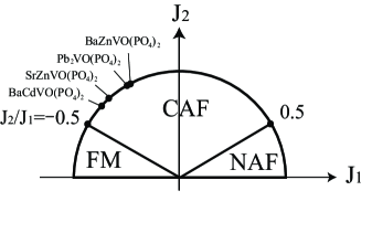
Figure 1: Classical phase diagram of the $J_{1}$-$J_{2}$ square lattice model [Eq. 2] for $J_{2}>0$ and ${\text{H}}=0$. FM, NAF, and CAF stand for ferromagnetic, Néel antiferromagnetic, and collinear anti-ferromagnetic phases. The spin configuration of each phase is shown in Fig. 2. Also shown are the experimentally determined exchange parameters of several materials [14] whose magnetic properties are well described by $H_{2d}$ [Eq. 2]: $J_{2}/J_{1}=-0.9$ for BaCdVO(PO₄)₂; $J_{2}/J_{1}=-1.1$ for SrZnVO(PO₄)₂; $J_{2}/J_{1}=-1.8$ for Pb₂VO(PO₄)₂; $J_{2}/J_{1}=-1.9$ for BaZnVO(PO₄)₂. In the $S=1/2$ quantum case, for $J_{2}/|J_{1}|\gtrsim 0.4$ and $J_{1}<0$, the spin nematic phase is theoretically expected slightly below the saturation phase[3, 10]

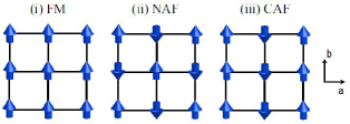
Figure 2: (Color online) Spin configurations of the classical ground states of $H_{2d}$ [Eq. 2] at ${\text{H}}=0$ (see Fig. 1).

In any real compound, there is always a finite interlayer coupling. This is the case for BaCdVO(PO₄)₂, SrZnVO(PO₄)₂, Pb₂VO(PO₄)₂ and BaZnVO(PO₄)₂. Naively, this would tend to destabilize non-trivial quantum phases, and thus, in order to guide the experimental search for the spin-nematic state, it is important to study the effect of interlayer coupling. The role of interlayer coupling on $H_{2d}$ [Eq. 2] has been studied in the classical CAF, and Néel antiferromagnetic (NAF) phases, as well as in the quantum disordered phase near the CAF/NAF boundary [9, 20, 21, 22, 23]. However, to our knowledge, it has not been studied in the spin-nematic phase. This is unlike the case of quasi-1D $J_{1}$-$J_{2}$ chains, where the stability of the spin-nematic state to interlayer coupling has been studied extensively [24, 26, 27, 28, 29, 25, 30, 31].

In this Letter, we study the effect of interlayer coupling on $H_{2d}$ [Eq. 2] close to the CAF/FM phase boundary in high magnetic field, fully taking into account quantum fluctuations. We consider a cubic lattice formed from $J_{1}$-$J_{2}$ planes with interlayer coupling $J_{\text{C}}$ (see Fig. 3). We determine the phase diagram just below the saturation field using the dilute-Bose-gas and Bethe-Salpeter (bound-magnon) methods [11, 32, 33, 25]. We find that the spin-nematic state is robust close to the classical CAF/FM boundary ($J_{2}/J_{1}\sim-0.5$), and is the ground state even for $|J_{\text{C}}/J_{1}|\sim 1$. At higher values of $J_{2}/J_{1}$, the spin-nematic state is destabilized by large interlayer coupling $|J_{\text{C}}|$, and we find a sizeable region of parameter space where a phase-separated state is expected. For large values of $|J_{\text{C}}|$ the semiclassically expected canted-CAF phase appears.

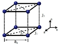
Figure 3: (Color online) Three-dimensional stacked-square (cubic) lattice. Filled spheres denote spins connected by Heisenberg exchange interactions. $J_{1}$ ($J_{2}$) describes the (next) nearest-neighbor exchange interaction in the a-b plane. The interlayer coupling is given by $J_{\text{C}}$. We set the lattice constant $a_{0}=1$.

Hamiltonian- We study the stacked $J_{1}$-$J_{2}$ Heisenberg model on the square lattice with interlayer coupling $J_{\text{C}}$ (i.e the cubic lattice, see Fig. 3),

$$\begin{split}H=&\sum_{\text{n.n in a-b}}J_{1}{\bf S}_{\mathbf{i}}\cdot{\bf S}_{\mathbf{j}}+\sum_{\text{n.n.n in a-b}}J_{2}{\bf S}_{\mathbf{i}}\cdot{\bf S}_{\mathbf{i}^{\prime}}+\sum_{\mathbf{l}}J_{\text{C}}{\bf S}_{\mathbf{i}}\cdot{\bf S}_{\mathbf{j}+\mathbf{e}_{c}}\\ &+{\text{H}}\sum_{\mathbf{l}}S^{z}_{\mathbf{l}}\ ,\end{split}$$ (2)

where ‘n.n. (n.n.n.) in a-b’ implies (next) nearest-neighbor couplings in the a-b plane.

We use the hardcore-boson representation,

$$S^{z}_{l}=-1/2+a^{\dagger}_{l}a_{l}\;,\;\;S_{l}^{+}=a_{l}^{\dagger}\;,\;\;S_{l}^{-}=a_{l}\;,$$ (3)

$$\begin{split}H&=\sum_{q}(\omega(\mathbf{q})-\mu)a^{\dagger}_{\mathbf{q}}a_{\mathbf{q}}+\frac{1}{2N}\sum_{\mathbf{q},\mathbf{k},\mathbf{k}^{\prime}}V_{\mathbf{q}}a_{\mathbf{k}+\mathbf{q}}^{\dagger}a_{\mathbf{k}^{\prime}-\mathbf{q}}^{\dagger}a_{\mathbf{k}}a_{\mathbf{k}^{\prime}},\\ &\omega(\mathbf{q})=\epsilon(\mathbf{q})-\epsilon_{\text{min}}\ ,\ \ \ \mu={\rm H}_{\text{c}}-{\rm H}\ ,\\ &{\rm H}_{\text{c}}=\epsilon({\bf 0})-\epsilon_{\text{min}}\ ,\ \ \ V_{\mathbf{q}}=2(\epsilon(\mathbf{q})+U)\ ,\end{split}$$ (4)

where the on-site interaction $U\rightarrow\infty$ and,

$$\begin{split}\epsilon({\bf q})&=J_{1}(\cos q_{a}+\cos q_{b})+J_{2}(\cos(q_{a}+q_{b})+\cos(q_{a}-q_{b}))\\ &+J_{\text{C}}\cos q_{c}\ ,\end{split}$$ (5)

with $\epsilon_{min}$ the minimum of $\epsilon(\mathbf{q})$:

(i) For $-2\leq J_{1}/J_{2}\leq 2$ and $J_{2}>0$: $\epsilon_{min}=\epsilon(\mathbf{Q}_{\pm}^{(f,a)})=-2J_{2}-|J_{\text{C}}|$, where the labels (f) and (a) are respectively chosen for $J_{\text{C}}<0$ and $J_{\text{C}}>0$. $\mathbf{Q}_{+}^{(f)}=(\pi,0,0)$, $\mathbf{Q}_{-}^{(f)}=(0,\pi,0)$, $\mathbf{Q}_{+}^{(a)}=(\pi,0,\pi)$ and $\mathbf{Q}_{-}^{(a)}=(0,\pi,\pi)$.

(ii) For $J_{1}/J_{2}\leq-2$ and $J_{2}>0$: $\epsilon_{min}=\epsilon(\mathbf{Q}_{f}^{(f,a)})=2J_{1}+2J_{2}-|J_{\text{C}}|$, where $\mathbf{Q}_{f}^{(f)}=(0,0,0)$ and $\mathbf{Q}_{f}^{(a)}=(0,0,\pi)$.
Here ${\text{H}}_{c}$ is the saturation field. If the field is reduced below $\text{H}_{c}$, the magnon gap closes ($\mu>0$), and magnon-Bose-Einstein condensation may occur.

GL Analysis- We focus here on the case $-2\leq J_{1}/J_{2}\leq 2$ and $J_{2,3}>0$. An equivalent analysis can be made for $J_{\text{C}}<0$. Slightly below the saturation field, and for $\mu>0$, Bose-Einstein condensation of magnons may occur at two momenta,

$$\langle a_{\mathbf{Q}_{+}^{(a)}}\rangle =\sqrt{N\rho_{\mathbf{Q}_{+}}}\exp(i\theta_{\mathbf{Q}_{+}}),$$ (6)

$$\langle a_{\mathbf{Q}_{-}^{(a)}}\rangle =\sqrt{N\rho_{\mathbf{Q}_{-}}}\exp(i\theta_{\mathbf{Q}_{-}}).$$ (7)

The induced spin-ordered phase is characterized by the wave vectors $\mathbf{Q}_{+}^{(a)}$ and/or $\mathbf{Q}_{-}^{(a)}$.

In the dilute limit, the energy density $E/N$ is expanded in the density $\rho_{{\bf Q}_{\pm}}$. Retaining terms up to quadratic order gives,

$$\frac{E}{N}= \frac{\Gamma_{1}}{2}\left(\rho_{\mathbf{Q}_{+}}^{2}+\rho_{\mathbf{Q}_{-}}^{2}\right)+[\Gamma_{2}+\Gamma_{3}\cos 2(\theta_{\mathbf{Q}_{+}}-\theta_{\mathbf{Q}_{-}})]\rho_{\mathbf{Q}_{+}}\rho_{\mathbf{Q}_{-}}$$

$$-\mu(\rho_{\mathbf{Q}_{+}}+\rho_{\mathbf{Q}_{-}}).$$ (8)

Here we introduced the renormalized interactions $\Gamma_{1}$, which acts between bosons of the same species, $\Gamma_{2}$ which acts between different species, and $\Gamma_{3}$, which describes umklapp scattering.

$\Gamma_{1,2,3}$ are determined from the scattering amplitude shown in Fig. 4,

$$\begin{split}&\Gamma(\Delta,\mathbf{K};\mathbf{p},\mathbf{p}^{\prime})=V(\mathbf{p}^{\prime}-\mathbf{p})+V(-\mathbf{p}^{\prime}-\mathbf{p})\\ &-\frac{1}{2}\int\frac{d^{3}p^{\prime\prime}}{(2\pi)^{3}}\frac{\Gamma(\Delta,\mathbf{K};\mathbf{p},\mathbf{p}^{\prime\prime})[V(\mathbf{p}^{\prime}-\mathbf{p}^{\prime\prime})+V(-\mathbf{p}^{\prime}-\mathbf{p}^{\prime\prime})]}{\omega(\mathbf{K}/2+\mathbf{p}^{\prime\prime})+\omega(\mathbf{K}/2-\mathbf{p}^{\prime\prime})+\Delta-i0^{+}},\end{split}$$ (9)

where the integral is taken over the region $p^{\prime\prime}_{x,y,z}\in(0,2\pi)$. $\mathbf{K}$ is the center-of-mass momentum of the two magnons and $\Delta$ is the binding energy. We solve this integral exactly [11, 32, 33, 25].

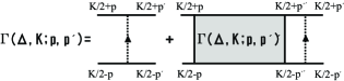
Figure 4: (Color online) Ladder diagram for the scattering amplitude $\Gamma$ [Eq. 9].

As a result, we obtain

$$\begin{split}\Gamma_{1}&=\Gamma(0,2\mathbf{Q}_{+}^{(a)};0,0)/2\ ,\\ \Gamma_{2}&=\Gamma(0,\mathbf{q}_{1};\mathbf{q}_{2},\mathbf{q}_{2})\ ,\\ \Gamma_{3}&=\Gamma(0,2\mathbf{Q}_{+}^{(a)};0,\mathbf{q}_{0})/2\ ,\end{split}$$ (10)

where $\mathbf{q}_{0}=(\pi,\pi,0)$, $\mathbf{q}_{1}=(\pi,\pi,2\pi)$, and $\mathbf{q}_{2}=(\pi/2,-\pi/2,0)$.

The values of $\Gamma_{1,2,3}$ determine the nature of the emergent phase for $\mu>0$. When $\Gamma_{1}<\Gamma_{2}-|\Gamma_{3}|$ and $\Gamma_{1}>0$, $\rho_{Q_{+}}=\rho=\frac{\mu}{\Gamma_{1}}$ and $\rho_{Q_{-}}=0$ (or vice versa). When the magnon at the wavevector $\mathbf{Q}_{+}^{(a)}$ condenses as,

$$\langle a_{l}\rangle=\sqrt{\rho}\exp[i({\bf Q_{+}^{(a)}}{\cdot}{\bf R}_{l}+\theta_{\mathbf{Q}_{+}})],$$ (11)

the spin-expectation values are given by,

$$\begin{split}&\langle S_{l}^{z}\rangle=-\frac{1}{2}+\rho\ ,\\ &\langle S_{l}^{x}\rangle=\sqrt{\rho}\cos({\bf Q_{+}^{(a)}}{\cdot}{\bf R}_{l}+\theta_{\mathbf{Q}_{+}})\ ,\\ &\langle S_{l}^{y}\rangle=-\sqrt{\rho}\sin({\bf Q_{+}^{(a)}}{\cdot}{\bf R}_{l}+\theta_{\mathbf{Q}_{+}}).\\ \end{split}$$ (12)

This describes the canted-CAF phase, in agreement with predictions from large-$S$ spin-wave theory via the order-by-disorder mechanism [34, 35].

If $\Gamma_{1}>\Gamma_{2}-|\Gamma_{3}|$, $\Gamma_{1}>0$ and $\Gamma_{1}+\Gamma_{2}-|\Gamma_{3}|>0$, $\rho_{Q_{+}}=\rho_{Q_{-}}=\rho^{\prime}=\frac{\mu}{\Gamma_{1}+\Gamma_{2}-|\Gamma_{3}|}$. In this case, we expect a nontrivial multiple-Q (double-Q) phase, which is also observed in several other models[25, 33, 36, 37, 38, 39, 40, 41, 42, 43]. However, these values of $\Gamma_{1,2,3}$ are not realised in $H$ [Eq. 2].

When $\Gamma_{1}<0$ or $\Gamma_{1}+\Gamma_{2}-|\Gamma_{3}|<0$, the dilutely-condensed phase is unstable, and a jump in the magnetization curve (phase separation) is expected at $\mu<0$.[11] This follows from the divergence of $E/N$ [Eq. 8], which is in turn due to the lack of higher-order interaction terms. For example, if $\Gamma_{1}<0$, it can be seen that $E/N\to-\infty$ if $\rho_{\mathbf{Q}}\to\infty$.

Bound Magnon- We have discussed the magnetic phases induced by single magnon condensation just below the saturation field. The other possibility is that magnons form stable-bound states, and the gap to the bound magnon closes at higher field than that of the single magnon. As a consequence, the bound magnon can condense, leading to spin-nematic state with a director order parameter perpendicular to the field. The order parameter is given by $\langle S^{\pm}\rangle_{i}=0$, $\langle S^{+}_{i}S^{+}_{j}\rangle\neq 0$.

The binding energy and the wavefunction of the two-magnon bound state can be understood from the scattering amplitude $\Gamma$. The divergence of $\Gamma$ implies a stable bound state with binding energy $\Delta_{B}(\mathbf{K})$. If the largest binding energy has $\Delta_{\text{min}}>0$, the bound state will condense when $\text{H}<\text{H}_{c2}=\text{H}_{c}+\Delta_{\text{min}}/2$. The wavefunction of the bound state follows from the residue of $\Gamma$.[13]

Phase Diagram- By calculating $\Gamma_{1,2,3}$ numerically, we obtain the phase diagram slightly below the saturation field, and this is shown in Figs. 5,6. In the yellow region (i), the bound magnon is the leading instability of the fully polarized phase. [44] Near the classical CAF/FM phase boundary ($J_{2}/|J_{1}|\sim 0.5$), the spin-nematic phase exists even at $|J_{\text{C}}/J_{1}|\sim 1$.

In the blue region (ii), $\Gamma_{1}<0$, and a phase separation is expected. In consequence, there is a magnetization jump when the magnetic field is lowered through the saturation value. It is beyond the scope of this Letter to predict which phase occurs below saturation, since the first-order-phase transition introduces a finite density of magnons, and the dilute Bose gas approximation breaks down.

For $\Gamma_{1}<\Gamma_{2}-|\Gamma_{3}|$, a naive approach that neglects the effect of finite density suggests the 1st-order phase transition to canted CAF with an associated jump in the magnetization. However, we cannot exclude the possibility that a spin-nematic phase or a double-Q phase is stabilized by interaction effects. On the boundary of the (i) nematic and (ii) phase separation regions, the s-wave scattering amplitude $\Gamma_{1}$ diverges, and, close to this boundary, the Efimov effect is expected [45].

In the (iii) red region, single magnons condense and form a canted-CAF phase. The phase (i), (ii) and (iii) span the entire region where the canted-CAF phase is expected semiclassically ($-2<J_{1}/J_{2}<2$ and $J_{2}>0$, see Fig. 1). For $0<J_{1}/J_{2}<2$ and $J_{1}>0$ the first instability of the saturated paramagnet is always to the canted-CAF phase. This is true even in the highly frustrated region $J_{1}/J_{2}\sim 2$ (classical CAF-NAF phase boundary in Fig. 1).

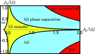
Figure 5: (Color online) Phase diagram of $H$ [Eq. 2] slightly below the saturation field and with $J_{1}<0$. The phases are: (i) spin nematic; (ii) phase separation (1st-order phase transition); (iii) canted-CAF phase (expected from the large-S expansion). In the unlabeled white region, the trivial FM (antiferromagnetic phase along $c$-axis) is expected for $J_{\text{C}}<0$ ($J_{\text{C}}>0$).

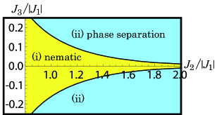
Figure 6: (Color online) Expanded view of Fig. 5 at small $J_{\text{C}}/|J_{1}|$.

Conclusion- We have studied the effect of interlayer coupling, $J_{\text{C}}$, on the magnetic phase diagram of the $S=1/2$ stacked-square-lattice $J_{1}$-$J_{2}$ model under high external field, using the dilute Bose-gas technique.[32, 13] The main result, shown in Figs. 5,6, is the phase diagram just below the saturation field. While semi-classical theory always predicts a canted CAF phase, a full quantum treatment reveals the presence of spin-nematic and phase separated regions. The spin-nematic state, which has previously been shown to exist in the pure 2D model ($J_{\text{C}}=0$) [3], is robust against the addition of interlayer coupling in the vicinity of the FM/CAF phase boundary ($J_{2}/J_{1}\sim-0.5$). For larger values of $J_{2}/|J_{1}|$ a broad phase-separation region is stabilized by the addition of $J_{\text{C}}$ coupling. Here a magnetization jump is expected as field is lowered through the saturation value, and, below this jump, the canted CAF-phase is expected to appear, although interactions may favor a spin nematic or double-Q phase. On the boundary between the spin-nematic phase and the phase separated region, the s-wave scattering amplitude $\Gamma_{1}$ diverges and the Efimov effect is expected.[45] The final conclusion is that in a quasi-2D, $J_{1}$-$J_{2}$ compound with $J_{1}<0$ and $J_{2}/|J_{1}|\gtrsim 0.5$, close to the saturation magnetic field the spin nematic state is remarkably robust against interlayer coupling.

The author thanks N. Shannon and A. Smerald for useful discussions and careful readings of this Letter. In addition, the author appreciates the helpful English corrections of this Letter by A. Smerald. The author is also grateful to supports by Okinawa Institute of Science and Technology, and JSPS KAKENHI Grant No. 26800209.

References

- [1] A. F. Andreev and A. Grishchuk, Sov. Phys. JETP 60, 267 (1984).
- [2] K. Penc and A. Lauchli, Chap. 13, Introduction to frustrated magnetism, edited by C. Lacroix, P. Mendels, F. Mila (Springer-Verlag Berlin Heidelberg 2011).
- [3] N. Shannon, T. Momoi, and P. Sindzingre, Phys. Rev. Lett. 96, 027213 (2006).
- [4] J. Richter, R. Darradi, J. Schulenburg, D. J. J. Farnell, and H. Rosner, Phys. Rev. B 81, 174429 (2010).
- [5] H. Feldner, D. C. Cabra, and G. L. Rossini, Phys. Rev. B 84, 214406 (2011).
- [6] R. Shindou and T. Momoi, Phys. Rev. B 80, 064410 (2009).
- [7] H. T. Ueda and K. Totsuka, Phys. Rev. B 76, 214428 (2007).
- [8] R. Shindou, S. Yunoki, and T. Momoi, Phys. Rev. B 84, 134414 (2011).
- [9] P. Thalmeier, M. E. Zhitomirsky, B. Schmidt, and N. Shannon, Phys. Rev. B 77, 104441 (2008).
- [10] In Ref. \citenSquareNem, the parameter range of where the spin nematic phase appears slightly below the saturation field is not declared explicitly. The concrete parameter is reproduced in Ref. \citenUeda_Momoi and in this letter.
- [11] H. T. Ueda and T. Momoi, Phys. Rev. B 87, 144417 (2013).
- [12] D. C. Mattis, The Theory of Magnetizm Made Simple, World Scientific, Singapore, (2006).
- [13] N. Nakanishi, Suppl. Prog. Theor. Phys, 43, 1, (1969); For review in the spin-system case, see Appendix in Ref. \citenUeda_Momoi.
- [14] R. Nath, A. A. Tsirlin, H. Rosner, and C. Geibel, Phys. Rev. B 78, 064422 (2008).
- [15] A. A. Tsirlin and H. Rosner, Phys. Rev. B 79, 214417 (2009).
- [16] A. A. Tsirlin, B. Schmidt, Y. Skourski, R. Nath, C. Geibel, and H. Rosner, Phys. Rev. B 80, 132407 (2009).
- [17] N. Oba, H. Kageyama, T. Kitano, J. Yasuda, Y. Baba, M. Nishi, K. Hirota, Y. Narumi, M. Hagiwara, K. Kindo, T. Saito, Y. Ajiro, and K. Yoshimura, J. Phys. Soc. Jpn. 75, 113601 (2006); Y. Tsujimoto, A. Kitada, H. Kageyama, M. Nishi, Y. Narumi, K. Kindo, Y. Kiuchi, Y. Ueda, Y. J. Uemura, Y. Ajiro, and K. Yoshimura, J. Phys. Soc. Jpn. 79, 014709 (2010).
- [18] M. Sato, T. Momoi, and A. Furusaki, Phys. Rev. B 79, 060406(R) (2009).
- [19] A. Smerald and N. Shannon, Phys. Rev. B 88, 184430 (2013).
- [20] D. Schmalfuß, R. Darradi, J. Richter, J. Schulenburg, and D. Ihle, Phys. Rev. Lett. 97, 157201 (2006).
- [21] M. Holt, O. P. Sushkov, D. Stanek, and G. S. Uhrig, Phys. Rev. B 83, 144528 (2011).
- [22] W. Nunes, J. R. Viana and J. R. Sousa, J. Stat. Mech. P05016 (2011).
- [23] K. Majumdar, J. Phys.: Cond. Mat. 23, 116004 (2011).
- [24] R. O. Kuzian and S.-L. Drechsler, Phys. Rev. B 75 024401 (2007).
- [25] H. T. Ueda and K. Totsuka, Phys. Rev. B 80, 014417 (2009).
- [26] M. E. Zhitomirsky and H. Tsunetsugu, Europhys. Lett. 92, 37001 (2010).
- [27] S. Nishimoto, et. al. Phys. Rev. Lett. 107, 097201 (2011).
- [28] A. V. Syromyatnikov, Phys. Rev. B 86, 014423 (2012).
- [29] M. Sato, T. Hikihara, and T. Momoi, Phys. Rev. Lett, 110, 077206 (2013).
- [30] O. A. Starykh and L. Balents, Phys. Rev. B 89, 104407 (2014).
- [31] H. T. Ueda and K. Totsuka, arXiv: 1406.1960
- [32] E. G. Batyev and L. S. Braginskii, Zh. Eksp. Teor. Fiz. 87, 1361 (1984) [Sov. Phys. JETP 60, 781 (1984)]; E. G. Batyev, Zh. Eksp. Teor. Fiz. 89, 308 (1985) [Sov. Phys. JETP 62, 173 (1985)].
- [33] T. Nikuni and H. Shiba, J. Phys. Soc. Jpn. 64, 3471 (1995).
- [34] E. F. Shender, Zh. Eksp. Teor. Fiz. 3, 326 (1982). [Sov. Phys. JETP 56, 178 (1982)].
- [35] C. L. Henley, Phys. Rev. Lett. 62, 2056 (1989).
- [36] M. Y. Veillette, J. T. Chalker, and R. Coldea, Phys. Rev. B 71, 214426 (2005).
- [37] Y. Kamiya and C. D. Batista, Phys. Rev. X 4, 011023 (2014).
- [38] G. Marmorini and T. Momoi, Phys. Rev. B 89, 134425 (2014).
- [39] O. A. Starykh, W. Jin, and A. V. Chubukov, Phys. Rev. Lett. 113, 087204 (2014).
- [40] M. Yamanaka, W. Koshibae, and S. Maekawa, Phys. Rev. Lett. 81, 5604 (1998).
- [41] I. Martin and C. D. Batista, Phys. Rev. Lett. 101, 156402 (2008).
- [42] Y. Akagi and Y. Motome, J. Phys. Soc. Jpn. 79, 083711 (2010); Y. Akagi, M. Udagawa, and Y. Motome, Phys. Rev. Lett. 108, 096401 (2012).
- [43] S. Hayami, T. Misawa, Y. Yamaji, and Y. Motome, Phys. Rev. B 89, 085124 (2014).
- [44] We do not exclude the possibility of the 1st-order phase transition at the saturation field even in the yellow region (i). It happens if the not-evaluated interaction between the bound magnon is negative. Actually, for at , the 36-sites exact diagonalization suggests the 1st-order phase transition to the nematic phase at the saturation field[3]. Hence, in our stacked-lattice case for , we may expect the 1st-order phase transition to the nematic phase for in the yellow region (i).
- [45] Y. Nishida, Y. Kato, C. D. Batista, Nature Physics 9, 93 (2013).