Probing WIMP particle physics and astrophysics with direct detection and neutrino telescope data

Abstract

With positive signals from multiple direct detection experiments it will, in principle, be possible to measure the mass and cross sections of weakly-interacting massive particle (WIMP) dark matter. Recent work has shown that, with a polynomial parameterisation of the WIMP speed distribution, it is possible to make an unbiased measurement of the WIMP mass, without making any astrophysical assumptions. However, direct detection experiments are not sensitive to low-speed WIMPs and, therefore, any model-independent approach will lead to a bias in the cross section. This problem can be solved with the addition of measurements of the flux of neutrinos from the Sun. This is because the flux of neutrinos produced from the annihilation of WIMPs which have been gravitationally captured in the Sun is sensitive to low-speed WIMPs. Using mock data from next-generation direct detection experiments and from the IceCube neutrino telescope, we show that the complementary information from IceCube on low-speed WIMPs breaks the degeneracy between the cross section and the speed distribution. This allows unbiased determinations of the WIMP mass and spin-independent and spin-dependent cross sections to be made, and the speed distribution to be reconstructed. We use two parameterisations of the speed distribution: binned and polynomial. While the polynomial parameterisation can encompass a wider range of speed distributions, this leads to larger uncertainties in the particle physics parameters.

I Introduction

Experiments aiming at detecting dark matter (DM) directly rely on measuring the signatures left by DM particles when they interact with the nuclei of a detector Cerdeno and Green (2010); Strigari (2013). This technique was devised to search for a specific class of DM candidates: Weakly Interacting Massive Particles (WIMPs) Goodman and Witten (1985). WIMPs characteristically have a mass of the order of GeV to TeV, and their elastic scatterings off target nuclei induce recoils with energy on the order of keV.

The number and energies of the recoil events can in principle be used to infer the properties of the DM particle, e.g. its mass and scattering cross sections. However, with a single experiment, this requires knowledge of the local WIMP velocity distribution, $f(\mathbf{v})$ (e.g. Ref. Peter (2011)). Data analyses usually use the so-called Standard Halo Model (SHM), where the velocity distribution is assumed to have the following simple form (in the Galactic rest frame):

$$f_{\textrm{Gal}}(\textbf{v})=\frac{1}{(2\pi\sigma_{v}^{2})^{3/2}}\exp\left(-\frac{\textbf{v}^{2}}{2\sigma_{v}^{2}}\right)\,.$$ (1)

This corresponds to an isothermal, spherical DM halo with density profile $\rho(r)\propto r^{-2}$, in equilibrium, in which case the dispersion $\sigma_{v}$ is related to the local circular speed $v_{c}\approx 220\textrm{ km s}^{-1}$ Feast and Whitelock (1997); Bovy et al. (2012) by $\sigma_{v}=v_{c}/\sqrt{2}$. The SHM velocity distribution is usually truncated manually at the Galactic escape speed, which we take to be $v_{\mathrm{esc}}=544\textrm{ km s}^{-1}$, consistent with the estimates from the RAVE survey Smith et al. (2007); Piffl et al. (2014).

Despite its simplicity and extensive use, it is unlikely that the SHM provides a good description of the DM velocity distribution. More realistic models have been proposed that allow for a triaxial DM halo Evans et al. (2000), a more general density profile Widrow (2000) and/or an anisotropic velocity distribution Bozorgnia et al. (2013). Furthermore, if the DM speed distribution is reconstructed self-consistently from the potential of the Milky Way Bhattacharjee et al. (2013); Fornasa and Green (2013) the resulting distribution deviates from the Maxwellian distribution of the SHM in Eq. (1).

Distribution functions extracted from $N$-body simulations also show deviations from the SHM Fairbairn and Schwetz (2009); Vogelsberger et al. (2009); Kuhlen et al. (2010); Mao et al. (2012). In particular, DM substructures (e.g. streams) may lead to ‘spikes’ in the speed distribution, while DM which has not yet completely phase-mixed (so-called ‘debris flows’) gives broad features Kuhlen et al. (2012). Simulations including baryonic physics suggest the possibility of a dark disk, produced by the DM tidally stripped from subhalos that are preferentially dragged into the stellar disk during the late stages of halo assembly Read et al. (2009, 2010). The resulting dark disk corotates with approximately the same speed as the stellar disk, but with a smaller velocity dispersion $\sigma_{v}\sim 50\textrm{ km s}^{-1}$. This dark disk may contribute an additional $20-100\%$ of the density of the halo (depending on the merger history of the Milky Way), although more recent simulations Pillepich et al. (2014) indicate a smaller density, $\sim 10\%$.

From the previous discussion it is clear that the velocity distribution is still a quite uncertain quantity, despite its fundamental importance in the interpretation of direct detection data Green (2012, 2010); McCabe (2010). Furthermore, probing the speed distribution would provide information on the structure and evolution of the Milky Way.

Various model independent techniques have recently been introduced for analysing direct detection data without rigid assumptions about the WIMP speed distribution, with the goal of obtaining unbiased constraints on the WIMP particle properties, e.g. Drees and Shan (2007); Strigari and Trotta (2009); Fox et al. (2011); Peter (2010, 2011); Feldstein and Kahlhoefer (2014). See Ref. Peter et al. (2014) for a review. In particular, Refs. Peter (2010, 2011) suggested employing an empirical parameterisation of the velocity distribution, and using data from multiple experiments to constrain its parameters along with the WIMP mass and cross section. Care must still be taken with the choice of parameterisation in order to avoid a biased determination of the WIMP mass Peter (2011); Kavanagh and Green (2012). We found that particular functional forms for the logarithm of $f(\mathbf{v})$, for instance Legendre and Chebyshev polynomials, allow an unbiased reconstruction of the WIMP mass Kavanagh and Green (2013); Kavanagh (2013); Peter et al. (2014). However, if only direct detection data is used, data analysis is inevitably hindered by the lack of sensitivity to low-speed WIMPs that produce recoil energies below the experimental energy thresholds. As experiments are blind to low-speed WIMPs, they can only detect some unknown fraction of the WIMPs. This then translates into a biased reconstruction of the scattering cross section.

Here we provide a solution to this problem using (simulated) future measurements from neutrino telescopes of the flux of neutrinos from the Sun. WIMPs scattering off the nucleons in the Sun can lose enough energy to get captured in its gravitational potential Press and Spergel (1985); Silk et al. (1985); Gaisser et al. (1986); Krauss et al. (1986); Srednicki et al. (1987); Griest and Seckel (1987). They accumulate there until their density is high enough to annihilate, producing (among other particles) neutrinos that can travel to us and be detected by neutrino telescopes, such as IceCube Ice . The expected number of neutrinos depends on the WIMP capture rate in the Sun, which is sensitive to the velocity distribution of WIMPs below a certain value.

A xenon-based direct detection experiment with ${\cal O}({\rm keV})$ energy threshold is sensitive to WIMPs with speeds above 500 $\textrm{ km s}^{-1}$ for light WIMPs with mass of order a few GeV, or above tens of $\textrm{ km s}^{-1}$ for heavier WIMPs. On the other hand, the maximum Solar capture speed (above which WIMPs are too fast to be captured) is larger than this for WIMP masses between 10 GeV and 1 TeV. Neutrino telescopes are therefore sensitive to the entire low-speed WIMP population which lies below the direct detection energy threshold. This indicates that combining direct detection and neutrino telescope data will allow us to probe the entire speed distribution and improve the accuracy of the constraints obtainable on both the WIMP mass and interaction cross section.

The complementarity of direct detection and neutrino telescope experiments has been studied previously in Ref. Arina et al. (2013). In that paper, astrophysical uncertainties were included by marginalising over parameters of the SHM, and by comparing with the results obtained assuming speed distributions from N-body simulations. In the current work, we account for such uncertainties using two general parametrisations of $f(v)$ described above, and investigate how well $f(v)$ can be reconstructed from data. Due to the degeneracy between the WIMP mass and speed distribution, such a general approach requires complementary information from several direct detection experiments, rather than a single experiment, as considered in Ref. Arina et al. (2013).

In the following sections we estimate the sensitivity of this general approach by means of Bayesian inference. We choose a set of well-motivated benchmarks for the mass and cross sections of the WIMP, as well as for its speed distribution. For each of these benchmarks we simulate the data expected in next-generation direct detection experiments and in a neutrino telescope. This data is encoded in a likelihood function, with which we scan over a parameter space that includes both particle physics quantities (e.g. the WIMP mass and scattering cross sections) and astrophysical ones (e.g. the coefficients entering in our parametrisation of the speed distribution). This technique allows us to estimate the precision with which future experiments will be able to reconstruct these parameters.

The paper is organized as follows. In Sec. II we summarize the formalism for the computation of recoil events in a direct detection experiment, as well as the expected signal in a neutrino telescope. In Sec. III we introduce the benchmark models considered and the parameterisations of the speed distribution. We also describe the sampling technique. In Sec. IV we present our results based on direct detection data only, while in Sec. V we also include the information from a neutrino telescope. Finally, we discuss our results in Sec. VII and summarize our main conclusions in Sec. VIII.

II Dark matter event rate formalism

II.1 Direct detection

The differential event rate per unit time and detector mass for nuclear recoils of energy $E_{\rm R}$ in a direct detection experiment is given by Jungman et al. (1995)

$$\frac{\textrm{d}R}{\textrm{d}E_{R}}=\frac{\rho_{0}}{m_{\chi}m_{\rm N}}\int_{v_{\mathrm{min}}}^{\infty}vf_{1}(v)\frac{\textrm{d}\sigma}{\textrm{d}E_{\rm R}}\,\mathrm{d}v\,.$$ (2)

The local DM mass density is denoted by $\rho_{0}$, the WIMP mass by $m_{\chi}$ and the target nuclear mass by $m_{\rm N}$. The prefactor $\rho_{0}/(m_{\chi}m_{\rm N})$ is the number of WIMPs per unit volume multiplied by the number of target nuclei per unit detector mass. The integral in Eq. (2) is of the differential cross section weighted by the one-dimensional WIMP speed distribution $f_{1}(v)$ (see later).

The WIMP velocity distribution in the Earth’s frame is related to that in the Galactic frame by a Galilean transformation: $f(\mathbf{v})=f_{\textrm{Gal}}(\textbf{v}-\textbf{v}_{\rm lag})$, where $\textbf{v}_{\rm lag}\approx 230\,{\rm km\,s^{-1}}$ is the velocity of the Earth with respect to the Galactic rest frame Lee et al. (2013); McCabe (2014). This includes a contribution from the velocity of the Sun with respect to the Galactic frame as well as a contribution from the Earth’s motion as it orbits the Sun. The dependence on the Earth’s orbit implies that the velocity distribution will be time-varying, producing an annual modulation in the event rate Freese et al. (1988). However, this modulation is expected to be $\lesssim 10\%$ and we consider here only the time averaged event rate. The one-dimensional speed distribution is obtained by integrating over all directions in the Earth frame

$$f_{1}(v)=\oint f_{\textrm{Gal}}(\textbf{v}-\textbf{v}_{\textrm{lag}})v^{2}\,\mathrm{d}\Omega_{\textbf{v}}\equiv v^{2}f(v)\,.$$ (3)

The function $f(v)$ is the directionally-averaged velocity distribution and is the quantity which we parametrise (and subsequently reconstruct) in order to account for astrophysical uncertainties.

The lower limit of the integral in Eq. (2) is the minimum WIMP speed that can excite a recoil of energy $E_{\rm R}$:

$$v_{\mathrm{min}}=\sqrt{\frac{m_{\rm N}E_{\rm R}}{2\mu_{\chi{\rm N}}^{2}}}\,,$$ (4)

where $\mu_{\chi{\rm N}}$ is the reduced mass of the WIMP-nucleon system.

The differential cross section is typically divided into spin-dependent (SD) and spin-independent (SI) contributions:

$$\frac{\textrm{d}\sigma}{\textrm{d}E_{\rm R}}=\frac{\textrm{d}\sigma_{{\rm SD}}}{\textrm{d}E_{\rm R}}+\frac{\textrm{d}\sigma_{{\rm SI}}}{\textrm{d}E_{\rm R}}\,.$$ (5)

The SI contribution can be written as

$$\frac{\textrm{d}\sigma_{{\rm SI}}}{\textrm{d}E_{\rm R}}=\frac{m_{\rm N}\sigma_{\mathrm{p}}^{\mathrm{SI}}}{2\mu_{\chi{\rm p}}^{2}v^{2}}A^{2}F_{{\rm SI}}^{2}(E_{\rm R})\,,$$ (6)

where we have assumed that the coupling to protons and neutrons is equal ($f_{\rm p}=f_{\rm n}$). In this case, the SI contribution scales with the square of the mass number $A$ of the target nucleus. The interaction strength is controlled by $\sigma_{\mathrm{p}}^{\mathrm{SI}}$, the WIMP-proton SI cross section, and by $\mu_{\chi{\rm p}}=m_{\chi}m_{\rm p}/(m_{\chi}+m_{\rm p})$, the reduced mass of the WIMP-proton system. The loss of coherence due to the finite size of the nucleus is captured in the form factor $F_{{\rm SI}}^{2}(E_{\rm R})$, which is obtained from the Fourier transform of the nucleon distribution in the nucleus. We take the form factor to have the Helm form Helm (1956)

$$F_{{\rm SI}}^{2}(E_{\rm R})=\left[\frac{3j_{1}(qR_{1})}{qR_{1}}\right]^{2}\mathrm{e}^{-q^{2}s^{2}}\,,$$ (7)

where $j_{1}(x)$ is a spherical Bessel function of the first kind and $q=\sqrt{2m_{\rm N}E_{\rm R}}$ is the momentum transfer. We use nuclear parameters from Ref. Lewin and Smith (1996), based on fits to muon spectroscopy data Fricke et al. (1995):

$$R_{1} =\sqrt{c^{2}+\frac{7}{3}\pi^{2}a^{2}-5s^{2}}\,,$$ (8)

$$c =1.23A^{1/3}-0.60\mbox{ fm}\,,$$ (9)

$$a =0.52\mbox{ fm}\,,$$ (10)

$$s =0.9\mbox{ fm}\,.$$ (11)

Muon spectroscopy probes the charge distribution in the nucleus. However, detailed Hartree-Fock calculations indicate that the charge distribution can be used as a good proxy for the nucleon distribution (especially in the case $f_{\rm p}=f_{\rm n}$). It has been shown that using the approximate Helm form factor introduces an error of less than $\sim$5% in the total event rate Duda et al. (2007); Co’ et al. (2012).

The standard expression for the SD contribution is

$$\frac{\textrm{d}\sigma_{{\rm SD}}}{\textrm{d}E_{\rm R}}=\frac{m_{\rm N}\sigma_{\mathrm{p}}^{\mathrm{SD}}}{2\mu_{\chi{\rm p}}^{2}v^{2}}\frac{4(J+1)}{3J}\left(\langle S_{\rm p}\rangle+\frac{a_{\rm n}}{a_{\rm p}}\langle S_{\rm n}\rangle\right)^{2}F_{{\rm SD}}^{2}(E_{\rm R})\,.$$ (12)

As before, $\sigma_{\mathrm{p}}^{\mathrm{SD}}$ denotes the WIMP-proton SD cross section and we have assumed that the coupling to protons and neutrons is equal ($a_{n}=a_{p}$). The total nuclear spin of the target is denoted $J$, while the expectation values of the proton and neutron spin operators are given by $\langle S_{\rm p}\rangle$ and $\langle S_{\rm n}\rangle$ respectively. The SD form factor can be written as

$$F_{{\rm SD}}^{2}(E_{\rm R})=\frac{S(E_{\rm R})}{S(0)}\,,$$ (13)

where $S(E_{\rm R})$ describes the energy dependence of the recoil rate due to the fact that the nucleus is not composed of a single spin but rather a collection of spin-1/2 nucleons. This response function $S(E_{\rm R})$ is usually decomposed in terms of spin structure functions Cannoni (2011):

$$S(E_{\rm R})=a_{0}^{2}S_{00}(E_{\rm R})+a_{0}a_{1}S_{01}(E_{\rm R})+a_{1}^{2}S_{11}(E_{\rm R})\,,$$ (14)

where $a_{0}=a_{\rm p}+a_{\rm n}$ is the isoscalar coupling and $a_{1}=a_{\rm p}-a_{\rm n}$ is the isovector coupling. Under the assumption $a_{\rm n}=a_{\rm p}$, then $a_{0}=2a_{\rm p}$ and $a_{1}=0$, and only the isoscalar structure function $S_{00}(E_{\rm R})$ will be relevant for our analysis.

The functional form for $S_{ij}$ can be calculated from shell models for the nucleus Ressell and Dean (1997). However, competing models (such as the Odd Group Model Engel and Vogel (1989), Interacting Boson Fermion Model Iachello et al. (1991) and Independent Single Particle Shell Model Ellis and Flores (1988), among others) may lead to different spin structure functions, generating a significant uncertainty in the value of the SD cross section. This issue was explored by Ref. Cerdeno et al. (2012), who developed a parametrisation for the spin structure functions in terms of the parameter $u=(qb)^{2}/2$, where

$$b=\sqrt{\frac{41.467}{(45.0A^{-1/3}-25.0A^{-2/3})}}\mbox{ fm}\,,$$ (15)

is the oscillator size parameter Warburton et al. (1990); Ressell and Dean (1997). Their parametrisation takes the form

$$S_{ij}=N((1-\beta)\mathrm{e}^{-\alpha u}+\beta)\,.$$ (16)

The values we use for the parameters $(N,\alpha,\beta)$ are $(0.0595,3.75,0.0096)$ for ¹²⁹Xe, $(0.035,3.925,0.12)$ for ¹³¹Xe and $(0.195,4.25,0.07)$ for ⁷³Ge. These values were chosen to approximately reproduce the median values obtained from a range of spin structure function calculations Ressell et al. (1993); Dimitrov et al. (1995); Ressell and Dean (1997); Menéndez et al. (2012). We keep the values of these parameters fixed in our analysis in order to focus on the impact of astrophysical uncertainties. We note that argon has zero spin and therefore has no SD interaction with WIMPs.

The proton and neutron spins $\langle S_{{\rm p},{\rm n}}\rangle$ can be rewritten in terms of the total nuclear spin and the spin structure functions (as in Ref. Cannoni (2013)). Using this to rewrite Eq. (12), gives the following expression (in the case $a_{p}=a_{n}$):

$$\frac{\textrm{d}\sigma_{\rm SD}}{\textrm{d}E_{R}}=\frac{8\pi m_{N}\sigma_{\mathrm{p}}^{\mathrm{SD}}}{3\mu_{\chi p}^{2}v^{2}}\frac{S_{00}(E_{R})}{(2J+1)}\,.$$ (17)

Both the SI and SD differential cross sections are inversely proportional to the WIMP velocity squared. Factoring out all the terms that do not depend on $v$ in Eq. (2), the integral over the WIMP speed is normally written as $\eta(v_{\rm min})$:

$$\eta(v_{\rm min})=\int_{v_{\rm min}}^{\infty}\frac{f_{1}(v)}{v}\mathrm{d}v\,,$$ (18)

and we will subsequently refer to this quantity as the velocity integral.

II.2 Neutrino telescopes

The WIMP capture rate per unit shell volume for a shell at distance $r$ from the center of the Sun, due to species $i$ is given by Gould (1987, 1992)

$$\frac{\textrm{d}C_{i}}{\textrm{d}V}=\int_{0}^{v_{\textrm{max}}}\textrm{d}v\,\frac{f_{1}(v)}{v}\,w\,\Omega^{-}_{w_{\textrm{esc}},i}(w)\,,$$ (19)

where $v$ is the asymptotic WIMP speed, $w(r)=\sqrt{v^{2}+w_{\rm esc}(r)^{2}}$ and $w_{\rm esc}(r)$ is the local escape speed at radius $r$ inside the Sun. The rate per unit time at which a single WIMP travelling at speed $w$ is scattered down to a speed less than $w_{\rm esc}$, due to the interaction with species $i$, is $\Omega^{-}_{w_{\rm esc},i}(w)$. Finally, the upper limit of integration is given by

$$v_{\mathrm{max}}=\frac{\sqrt{4m_{\chi}m_{{\rm N}_{i}}}}{m_{\chi}-m_{{\rm N}_{i}}}w_{\rm esc}\,,$$ (20)

where $m_{{\rm N_{i}}}$ is the mass of the nucleus of species $i$. Above $v_{\mathrm{max}}$, WIMPs cannot lose enough energy in a recoil to drop below the local escape speed and, therefore, they are not captured by the Sun.

The scatter rate $\Omega^{-}_{w_{\rm esc},i}$ from a species with number density $n_{{\rm N_{i}}}$ can be written as:

$$\Omega^{-}_{w_{\rm esc},i}(w)=w\,n_{{\rm N}_{i}}\int_{E_{v}}^{E_{\mathrm{max}}}\frac{\textrm{d}\sigma}{\textrm{d}E_{\rm R}}\,\mathrm{d}E_{\rm R}\,,$$ (21)

where $E_{\rm R}$ is the energy lost by the scattering WIMP. The limits of integration run from the minimum energy loss required to reduce the WIMP speed below $w_{\rm esc}$,

$$E_{v}=\frac{m_{\chi}}{2}\left(w^{2}-w_{\rm esc}^{2}\right)=\frac{m_{\chi}}{2}v^{2}\,,$$ (22)

to the maximum possible energy loss in the collision,

$$E_{\mathrm{max}}=\frac{2\mu_{\chi{\rm N}_{i}}^{2}}{m_{{\rm N}_{i}}}w^{2}\,.$$ (23)

As in the direct detection case, we can decompose the differential cross section into SI and SD components. While all of the constituent elements of the Sun are sensitive to SI interactions, only spin-1/2 hydrogen is sensitive to SD scattering. The differential cross section is therefore given by

$$\frac{\textrm{d}\sigma}{\textrm{d}E_{\rm R}}=\frac{m_{{\rm N}_{i}}}{2\mu_{\chi{\rm p}}^{2}v^{2}}\times\begin{cases}\sigma_{\mathrm{p}}^{\mathrm{SI}}+\sigma_{\mathrm{p}}^{\mathrm{SD}}&\textrm{ for }A=1\,,\\ \sigma_{\mathrm{p}}^{\mathrm{SI}}A_{i}^{2}F_{i}^{2}(E_{\rm R})&\textrm{ for }A>1\,.\end{cases}$$ (24)

No form factor is needed for hydrogen, which consists of only a single nucleon. For the remaining nuclei, we approximate the form factor as Gould (1987)

$$F^{2}_{i}(E_{\rm R}) =\exp{\left(-\frac{E_{\rm R}}{E_{i}}\right)}\,,$$ (25)

$$E_{i} =\frac{3}{2m_{{\rm N}_{i}}R_{i}^{2}}\,.$$ (26)

This allows Eq. (21) to be calculated analytically and introduces an error in the total capture rate of only a few percent.

Fig. 1 shows the maximum Solar capture speed $v_{\textrm{max}}$ given by Eq. (20) (averaged over the Solar radius). We consider separately the SD contribution (dashed red line) from hydrogen and the SI contribution (solid red line) averaged over all elements in the Sun. The former goes from a value slightly larger than 1000 $\textrm{ km s}^{-1}$ for a 10 GeV WIMP down to $\sim$ 100 $\textrm{ km s}^{-1}$ for a mass of 1 TeV, while the latter is larger by a factor of approximately two. The sharp peaks in the SI curve for $v_{\textrm{max}}$ are resonances due to mass matching between the WIMP and one of the nuclei in the Sun. In these cases, energy transfer during recoils can be very efficient and WIMPs with high speeds can be captured.

The two red lines should be compared with the blue (green hatched) band, which shows the velocity window to which a xenon-based (argon-based) experiment is sensitive (assuming the energy thresholds described in Sec. III and Tab. 1). We note that, over the whole range of masses considered, the maximum Solar capture speed is always larger (both for SI and SD interactions) than the lower edge of the blue band. This means that, as anticipated in the introduction, neutrino telescopes are sensitive to all of the low-speed tail of the velocity distribution that is inaccessible to direct detection experiments.

Figure 1: The ranges of WIMP velocity that Solar capture and direct detection experiments are sensitive to, as a function of the WIMP mass. The blue band shows the range of speeds to which a xenon-based detector with an energy window of $[5,45]$ keV is sensitive. The green hatched band shows the corresponding range of speeds for an argon-based detector with an energy window of $[30,100]$ keV. The solid (dashed) red lines shows the maximum speed to which Solar WIMP capture is sensitive for SI (SD) interactions. See the text for further details.

WIMPs which are captured can annihilate in the Sun to Standard Model particles. Over long timescales, equilibrium is reached between the capture and annihilation rates. In such a regime, the annihilation rate $\Gamma_{A}$ is equal to half the capture rate, independent of the unknown annihilation cross section Griest and Seckel (1987). For large enough scattering cross sections ($\sigma_{\mathrm{p}}^{\mathrm{SD}}\gtrsim 10^{-43}\textrm{ cm}^{2}$), capture is expected to be efficient enough for equilibrium to be reached Peter (2009). The assumption of equilibrium is, therefore, reasonable for the benchmarks considered in this work.

The majority of Standard Model particles produced by WIMP annihilations cannot escape the Sun. However, some of these particles may decay to neutrinos or neutrinos may be produced directly in the annihilation. Neutrinos can reach the Earth and be detected by neutrino telescope experiments. In this work, we focus on the IceCube experiment Aartsen et al. (2013a), which measures the Čerenkov radiation produced by high energy particles travelling through ice. IceCube aims at isolating the contribution of muons produced by muon neutrinos interacting in the Earth or its atmosphere. The amount of Čerenkov light detected, combined with the shape of the Čereknow cascade, allows the energy and direction of the initial neutrino to be reconstructed.

The spectrum of neutrinos arriving at IceCube is given by

$$\frac{\textrm{d}N_{\nu}}{\textrm{d}E_{\nu}}=\frac{\Gamma_{A}}{4\pi D^{2}}\sum_{f}B_{f}\frac{\textrm{d}N_{\nu}^{f}}{\textrm{d}E_{\nu}}\,,$$ (27)

where $D$ is the distance from the Sun to the detector and the sum is over all annihilation final states $f$, weighted by the branching ratios $B_{f}$. The factor $\mathrm{d}N_{\nu}^{f}/\mathrm{d}E_{\nu}$ is the neutrino spectrum produced by final state $f$, taking into account the propagation of neutrinos as they travel from the Sun to the detector Blennow et al. (2008); Baratella et al. (2014). The branching ratios depend on the specific WIMP under consideration. For simplicity, it is typically assumed (as we do here) that the WIMPs annihilate into a single channel. For the computation of Eq. (27) we use a modified version of the publicly available DarkSUSY code Gondolo et al. (2004, 2014), that also accounts for the telescope efficiency (see also Sec. III).

III Benchmarks and parameter reconstruction

In order to determine how well the WIMP parameters can be recovered, we generate mock data sets for IceCube and three hypothetical direct detection experiments.

Table 1 displays the parameters we use for the three direct detection experiments. They are chosen to broadly mimic next-generation detectors that are currently in development. Each experiment is described by the energy window it is sensitive to and the total exposure, which is the product of the fiducial detector mass, the exposure time and the experimental and operating efficiencies (which we implicitly assume to be constant). We also include a gaussian energy resolution of $\sigma_{E}=1\textrm{ keV}$  and a flat background rate of $10^{-7}$ events/kg/day/keV.

We choose three experiments using different target nuclei as it has been shown that the employment of multiple targets significantly enhances the accuracy of the reconstruction of the WIMP mass and cross sections Pato et al. (2011); Cerdeño et al. (2013); Cerdeno et al. (2014). Furthermore, if the WIMP velocity distribution is not known, multiple targets are a necessity Kavanagh and Green (2012). For more details on the reconstruction performance of different ensembles of target materials, we refer to reader the Ref. Peter et al. (2014). We note that our modelling of the detectors is rather unsophisticated. More realistic modelling would include, for instance, energy-dependent efficiency. However, the detector modelling we employ here is sufficient to estimate the precision with which the WIMP parameters can be recovered.

We divide the energy range of each experiment into bins and generate Asimov data Cowan et al. (2013) by setting the observed number of events in each bin equal to the expected number of events. While this cannot correspond to a physical realisation of data as the observed number of events will be non-integer, it allows us to disentangle the effects of Poissonian fluctuations from the properties of the parametrisations under study. Including the effect of Poissonian fluctuations would require the generation of a large number of realisations for each benchmark. The precision in the reconstruction of the WIMP parameters will, in general, be different for each realisation. This leads to the concept of coverage, i.e. how many times the benchmark value is contained in the credible interval estimating the uncertainty in the reconstruction (c.f. Ref. Strege et al. (2012)). We leave this for future work, noting here that Ref. Kavanagh (2013) showed that the polynomial parameterisation we use (Sec. III.2) provides almost exact coverage for the reconstruction of the WIMP mass (at least in the case of $m_{\chi}$ = 50 GeV).

Experiment	Energy Range (keV)	Exposure (ton-yr)	Energy bin width (keV)
Xenon	5-45	1.0	2.0
Argon	30-100	1.0	2.0
Germanium	10-100	0.3	2.0

Table 1: Summary of the parameters describing the mock direct detection experiments. All experiments have a constant energy resolution of $\sigma_{E}=1\textrm{ keV}$ and a flat background rate of $10^{-7}$ events/kg/day/keV. The energy windows are chosen to be similar to those proposed in Refs. Apr (2010); Bau (2013) and Grandi (2005) for xenon, germanium and argon respectively. We assume natural isotopic abundances of the target materials.

For the mock neutrino telescope data, we consider the IceCube 86-string configuration. We follow Ref. Arina et al. (2013) and use an exposure time of 900 days (corresponding to five 180-days austral Winter observing seasons) and an angular cut around the Solar position of $\phi_{\textrm{cut}}=3\,^{\circ}$. This value is chosen to reflect the typical angular resolution of the IceCube detector Danninger and Strahler (2011) and has previously been shown to be the optimal angular cut over a range of DM masses Silverwood et al. (2013). This results in approximately 217 background events over the full exposure. As with the direct detection experiments, we set the observed number of events equal to the expected number of signal plus background events. We use only the observed number of events as data and not their individual energies. While event-level likelihood methods have previously been developed Scott et al. (2012) for the use of IceCube 22-string data Abbasi et al. (2009), a similar analysis has not yet been performed for IceCube-86. In particular, the probability distributions for the number of lit digital optical modules as a function of neutrino energy are not yet available for IceCube-86. Nonetheless, using only the number of observed events is a first step towards the characterisation of the WIMP speed distribution with neutrino telescopes.

III.1 Benchmarks

The four benchmark models we use to generate mock data sets are summarised in Table 2, along with the number of events produced in each experiment. In all cases, we use a SI WIMP-proton cross section of $\sigma_{\mathrm{p}}^{\mathrm{SI}}=10^{-45}\textrm{ cm}^{2}$ and a SD cross section of $\sigma_{\mathrm{p}}^{\mathrm{SD}}=2\times 10^{-40}\textrm{ cm}^{2}$, both of which are close to the current best exclusion limits Akerib et al. (2014); Aprile et al. (2013).

Benchmark	$m_{\chi}\textrm{ (GeV)}$	Speed dist.	Annihilation channel	$N_{\mathrm{Xe}}(\mbox{SI})$	$N_{\mathrm{Xe}}(\mbox{SD})$	$N_{\mathrm{Ar}}(\mbox{SI})$	$N_{\mathrm{Ar}}(\mbox{SD})$	$N_{\textrm{Ge}}(\mbox{SI})$	$N_{\textrm{Ge}}(\mbox{SD})$	$N_{\textrm{IC}}$
A	100	SHM	$W^{+}W^{-}$	154.9	262.7	16.1	0	25.4	18.7	43.3
B	100	SHM+DD	$W^{+}W^{-}$	167.1	283.9	16.2	0	25.7	18.9	242.9
C	30	SHM	$\nu_{\mu}\bar{\nu}_{\mu}$	175.1	301.1	6.2	0	20.5	16.1	13.2
D	30	SHM+DD	$\nu_{\mu}\bar{\nu}_{\mu}$	175.0	300.9	5.8	0	20.4	16.0	40.2

Table 2: Summary of the WIMP benchmarks. The first section shows the WIMP mass, speed distribution and annihilation channel. SHM refers to the Standard Halo Model, with a speed distribution described by Eq. (1) with $v_{\textrm{lag}}=230\textrm{ km s}^{-1}$ and $\sigma_{v}=163\textrm{ km s}^{-1}$. In the case of SHM+DD, we also include the contribution of a dark disk, described by an additional term as in Eq. (1), but with $v_{\textrm{lag}}=50\textrm{ km s}^{-1}$ and $\sigma_{v}=50\textrm{ km s}^{-1}$. For all benchmarks, we consider only isospin-conserving interactions (i.e. $f_{\rm p}=f_{\rm n}$ and $a_{\rm p}=a_{\rm n}$) and assume $\sigma_{\mathrm{p}}^{\mathrm{SI}}=10^{-45}\textrm{ cm}^{2}$ and $\sigma_{\mathrm{p}}^{\mathrm{SD}}=2\times 10^{-40}\textrm{ cm}^{2}$. The second section gives the number of events produced in the xenon-, argon- and germanium-based direct detection experiments (with the number of recoils induced by SI and SD interactions listed separately) and IceCube.

The WIMPs in benchmarks A and B have an intermediate mass of 100 GeV and the production of neutrinos originates from annihilations into $W^{+}W^{-}$. This is a similar configuration to benchmark B used by Ref. Arina et al. (2013). For benchmarks C and D we decrease the mass to 30 GeV, which allows a more accurate reconstruction of the WIMP mass (see Secs. IV and V). The IceCube detector (with DeepCore) is sensitive to WIMPs with masses down to about 20 GeV Aartsen et al. (2013b). For benchmarks C and D we assume that annihilations take place directly into $\nu_{\mu}\bar{\nu}_{\mu}$.

Other annihilation channels may produce fewer neutrinos and, thus, reduce the impact of IceCube in the reconstruction of the particle physics nature of DM and its $f(v)$. However, note that, according to Ref. Cirelli et al. (2011), the only annihilation channels not decaying with a significant probability into neutrinos are electrons, gluons and gamma rays. The scan of non-minimal supersymmetry performed in Ref. Roszkowski et al. (2015) showed that these are subdominant channels.

Benchmarks A and C assume a SHM speed distribution as described in Sec. II, with $v_{\textrm{lag}}=230\textrm{ km s}^{-1}$ Schönrich (2012); Bovy et al. (2012) and $\sigma_{v}=163\textrm{ km s}^{-1}$. Benchmarks B and D also include a moderate dark disk with a population of low-speed WIMPs which contribute an additional 30% to the local DM density. We assume that the dark disk velocity distribution is also given by Eq. (1), with $v_{\textrm{lag}}=50\textrm{ km s}^{-1}$ and $\sigma_{v}=50\textrm{ km s}^{-1}$ Bruch et al. (2009). As shown in Ref. Choi et al. (2014), the capture rate in the Sun is not affected by variations in the shape of $f(v)$ (such as the differences between distribution functions extracted from different $N$-body simulations). However, significant enhancement of the capture rate can occur if there is a dark disk Bruch et al. (2009), and our benchmarks have been chosen in order to investigate this scenario. Finally, we assume a fixed value for the SHM local DM density of $\rho_{0}=0.3\textrm{ GeV cm}^{-3}$. There is an uncertainty in this value of around a factor of 2 (see e.g. Refs. Catena and Ullio (2010); Weber and de Boer (2010); Zhang et al. (2013); Nesti and Salucci (2013); Read (2014)). However this is degenerate with the cross sections.

In this work, we assume a common speed distribution $f(v)$ experienced by both Earth-based experiments and by the Sun. In principle gravitational focussing and diffusion could lead to differences between the forms of $f(v)$ at the Earth and Sun Gould (1991); Peter (2009). However, a recent study using Liouville’s theorem showed that such effects must be balanced by inverse processes Sivertsson and Edsjo (2012). We can, therefore, treat the WIMP population as being effectively free and consider only a single common form for $f(v)$.

III.2 Parametrisations of the speed distribution

We use the mock data generated for the benchmarks in Table 2 to evaluate the likelihood employed in the Bayesian scans over $m_{\chi}$, $\sigma_{\mathrm{p}}^{\mathrm{SI}}$ and $\sigma_{\mathrm{p}}^{\mathrm{SD}}$. In order to study the synergy between direct detection experiments and neutrino telescopes in the reconstruction of the speed distribution, some of these scans will also include parameters which describe the form of $f(v)$. We consider two possible parametrisations:

• Binned parametrisation: This parameterisation was introduced in Ref. Peter (2011) and it involves dividing $f(v)$ into $N$ bins of width $\Delta v$ with bin edges $\tilde{v}_{i}$ and parametrising the bin heights by ${g}_{i}$:

  $$f(v)=\sum_{i=1}^{N}\frac{3{g}_{i}\,W(v;\tilde{v}_{i},\Delta v)}{(\tilde{v}_{i}+\Delta v)^{3}-\tilde{v}_{i}^{3}}\,,$$ (28)

  where the top-hat function, $W$, is defined as:

  $$W(v;\tilde{v}_{i},\Delta v)=\begin{cases}1&v\in[\tilde{v}_{i},\tilde{v}_{i}+\Delta v]\,,\\ 0&\text{otherwise \,.}\end{cases}$$ (29)

  The bin heights then satisfy the normalisation condition

  $$\sum_{i=1}^{N}{g}_{i}=1\,.$$ (30)

  We parametrise $f(v)$ up to some maximum speed $v_{\textrm{max}}=N\Delta v$, above which we set $f(v)=0$. We choose $v_{\textrm{max}}=1000\textrm{ km s}^{-1}$, conservatively larger than the escape velocity in the Earth frame, which is around $800\textrm{ km s}^{-1}$ Smith et al. (2007); Piffl et al. (2014). The binned parametrisation was studied in detail in Ref. Kavanagh and Green (2012), where it was demonstrated that, when only direct detection data is used, this method results in a bias towards smaller WIMP masses.

• Polynomial parametrisation: In Ref. Kavanagh and Green (2013) we proposed that the natural logarithm of $f(v)$ be expanded in a series of polynomials in $v$, i.e.

  $$f(v)=\exp\left[\sum_{k=0}^{N-1}a_{k}P_{k}(2v/v_{\textrm{max}}-1)\right]\,.$$ (31)

  The first coefficent $a_{0}$ is fixed by requiring the speed distribution to be normalised to 1. As detailed in Ref. Kavanagh (2013), various polynomial bases can be used. Chebyshev and Legendre polynomials allow an unbiased reconstruction of the WIMP mass across a wide range of astrophysical and particle physics benchmarks Kavanagh and Green (2013); Kavanagh (2013), and the scans are normally faster if Chebyshev polynomials are used. We, therefore, use a basis of $N$ Chebyshev polynomials $P_{k}$ weighted by the parameters $a_{k}$.

By studying two different speed parametrisations, we can examine how particle physics parameter reconstruction is affected by the choice of speed parametrisation. While the binned parametrisation may lead to a bias in the WIMP mass, it is straight-forward and provides a good approximation to smoothly varying speed distributions. As discussed in Ref. Kavanagh and Green (2012), this bias is due in part to a lack of information about $f(v)$ at low speeds. We therefore expect that the addition of IceCube data will reduce this bias. By comparison, the polynomial distribution is unbiased and allows for a wider range of shapes for $f(v)$, although some of these are rapidly varying and may not be physically well-motivated. For a large number of parameters, these two methods should converge and both could be used as a consistency check.

III.3 Parameter sampling

We perform parameter scans using a modified version of the publicly available MultiNest 3.6 package Feroz and Hobson (2007); Feroz et al. (2008, 2013). This allows us to map out the likelihood $\mathcal{L}(\mathbf{\Theta})$ for the model parameters $\mathbf{\Theta}$. We use $N_{\textrm{live}}=20000$ live points and a tolerance of $10^{-4}$. The priors we use for the various parameters are displayed in Table 3.

Parameter	Prior range	Prior type
$m_{\chi}$ (GeV)	$10\--1000$	log-flat
$\sigma_{\mathrm{p}}^{\mathrm{SI}}\textrm{ (cm}^{2}\textrm{)}$	$10^{-48}\--10^{-42}$	log-flat
$\sigma_{\mathrm{p}}^{\mathrm{SD}}\textrm{ (cm}^{2}\textrm{)}$	$10^{-43}\--10^{-37}$	log-flat
Polynomial coefficients $\left\{a_{k}\right\}$	$-20\--20$	linear-flat
Bin heights $\left\{g_{i}\right\}$	$0\--1$	simplex

Table 3: Summary of prior types and ranges. The ‘simplex’ prior is described in Sec. III.3.

Due to the normalisation condition on the bin heights (given in Eq. (30)) for the case of the binned parametrisation of $f(v)$, we must sample these parameters from the so-called ‘simplex’ priors: i.e. we uniformly sample $\left\{g_{2},...,g_{N}\right\}$ such that they sum to less than one and then fix $g_{1}$ as

$$g_{1}=1-\sum_{i=2}^{N}{g}_{i}\,.$$ (32)

The ellipsoidal sampling performed by MultiNest becomes increasingly inefficient as the number of bins $N$ increases, since the volume of the parameter space for which Eq. (30) is satisfied becomes very small. We therefore use MultiNest in constant efficiency mode when using the binned parametrisation, with a target efficiency of 0.3. We use a total of 10 bins in this parameterisation (9 free parameters, with one fixed by normalisation), which should allow us to obtain a close approximation to the rapidly varying SHM+DD distribution.

For the polynomial $\ln f(v)$ parametrisation, we use 6 basis polynomials (5 free coefficients, with one fixed by normalisation). This is a smaller number of parameters than for the binned parameterisation because the polynomial coefficients are allowed to vary over a much wider range. The volume of the polynomial parameter space is therefore significantly larger than for the binned parametrisation and a much larger number of live points would be required to accurately map the likelihood using 10 parameters. As we will see, using 6 basis functions still allows a wide range of speed distributions to be explored and provides a good fit to the data (see also the discussion in Ref. Kavanagh (2013)). With a larger numbers of events, it would be feasible to increase the number of basis functions and more precisely parametrise the form of the speed distribution.

The likelihood function we use for each experiment is:

$$\mathcal{L}(\mathbf{\Theta})=\prod_{i=1,N_{\textrm{bins}}}\frac{(N_{\rm e}^{i})^{N_{\rm o}^{i}}}{N_{\rm o}^{i}!}e^{-N_{\rm e}^{i}}\,,$$ (33)

where the energy window is divided into $N_{\textrm{bins}}$ bins. For each bin, $N_{\rm e}^{i}$ is the expected number events, for a given set of parameters $\mathbf{\Theta}$, and $N_{\rm o}^{i}$ is the observed number of events (i.e. the mock data). The total likelihood is the product over the likelihoods for each experiment considered.

Finally, it is often interesting to consider the probability distribution of a subset of parameters from the full parameter space. We do this by profiling, so that the profile likelihood $\mathcal{L}_{p}(\theta_{i})$ of the $i$-th parameter is obtained by maximising $\mathcal{L}$ over the other parameters:

$$\mathcal{L}_{p}(\theta_{i})=\max\limits_{0,...,i-1,i+1,...,N}\mathcal{L}(\mathbf{\Theta})\,.$$ (34)

We have checked that, for the data sets and likelihoods used here, the marginalised posterior distributions of the parameters of interest do not differ qualitatively from the profile likelihood. We therefore do not display the marginalised posterior distributions. Because we only make use of the likelihood (and not the posterior distribution) in parameter inference, we expect that the priors will not strongly impact the results. In addition, the use of Asimov data with a large number of energy bins means that we expect the confidence intervals obtained from the asymptotic properties of the profile likelihood to be valid.

IV Direct detection data only

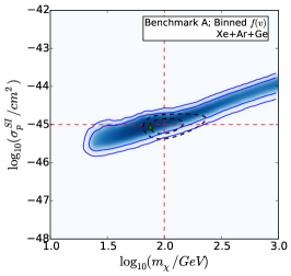
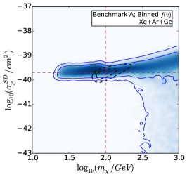
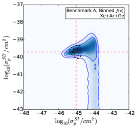
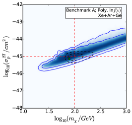
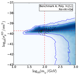
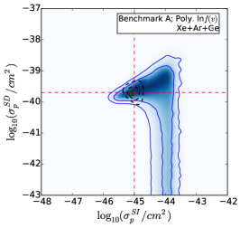
Figure 2: 2-dimensional profile likelihood for ($m_{\chi}$, $\sigma_{\mathrm{p}}^{\mathrm{SI}}$) (left column), ($m_{\chi}$, $\sigma_{\mathrm{p}}^{\mathrm{SD}}$) (central column) and ($\sigma_{\mathrm{p}}^{\mathrm{SI}}$, $\sigma_{\mathrm{p}}^{\mathrm{SD}}$) (right column), using only information from three direct detection experiments with Xenon, Germanium and Argon targets (see Tab. 1) for benchmark A. The shaded areas and solid blue contours are obtained from a scan of a parameter space that includes both the particle physics quantities ($m_{\chi}$, $\sigma_{\mathrm{p}}^{\mathrm{SI}}$ and $\sigma_{\mathrm{p}}^{\mathrm{SD}}$) and the parameters defining the speed distribution. The panels in the top row are for a binned parametrisation, while those in the second row are for a polynomial parametrisation (see Sec. III). The dashed black contours are from a separate scan, performed with the speed distribution fixed to its input form (see Tab. 2). In all cases, the inner (outer) contours enclose the 68% (95%) confidence level region. The green triangle marks the position of the best-fit point for the scan including the parameters of the speed distributions. The red dashed lines show the nominal values for $m_{\chi}$, $\sigma_{\mathrm{p}}^{\mathrm{SI}}$ and $\sigma_{\mathrm{p}}^{\mathrm{SD}}$ assumed for this benchmark.

In this section we present the results of the scans performed with only direct detection data, leaving the discussion of the impact of IceCube data for the following section.

IV.1 Benchmark A

Figure 2 shows the 2-dimensional profile likelihood distributions for benchmark A, i.e. $m_{\chi}$ =100 GeV, $\sigma_{\mathrm{p}}^{\mathrm{SI}}$ = $10^{-45}\textrm{ cm}^{2}$, $\sigma_{\mathrm{p}}^{\mathrm{SD}}$ = $2\times 10^{-40}\textrm{ cm}^{2}$ and a SHM $f(v)$. Left panels are for ($m_{\chi}$, $\sigma_{\mathrm{p}}^{\mathrm{SI}}$), central ones for ($m_{\chi}$, $\sigma_{\mathrm{p}}^{\mathrm{SD}}$), while the ones on the right are for ($\sigma_{\mathrm{p}}^{\mathrm{SI}}$, $\sigma_{\mathrm{p}}^{\mathrm{SD}}$). Shaded regions and solid blue contours are for scans carried out over particle physics quantities (i.e. $m_{\chi}$, $\sigma_{\mathrm{p}}^{\mathrm{SI}}$ and $\sigma_{\mathrm{p}}^{\mathrm{SD}}$) as well as the parameters entering in the parametrisation of the speed distribution. The first row is for the binned $f(v)$ and the second row for the polynomial expansion (see Sec. III.2). In addition, the dashed black contours are from a scan performed keeping the speed distribution fixed, i.e. assuming that the correct $f(v)$ is known and there are no astrophysical uncertainties.

In the case of a fixed speed distribution (dashed black lines), the reconstruction is very good: the mass is well constrained and closed contours are obtained for both the SI and SD cross section (right column). These constraints on the WIMP mass are similar to those obtained in Ref. Arina et al. (2013) whose Benchmark B is the same as our Benchmark A (see the middle row of Fig. 1 of Ref. Arina et al. (2013)). However, the possible degeneracy between the two cross sections Cerdeño et al. (2013), which is observed in Ref. Arina et al. (2013), is broken by the fact that we use three different target experiments, one of which (argon) is only sensitive to SI interactions.

When we allow for the realistic possibility of a variable speed distribution, the contours unsurprisingly increase in size. For both the binned and polynomial parametrisation, the contours have a similar shape, extending down to 20 – 30 GeV in $m_{\chi}$. This is because both parametrisations can encompass distributions that are flatter than the SHM. Decreasing the WIMP mass steepens the recoil spectrum, allowing these flatter distributions to be compatible with the mock data. An example of such a speed distribution is the one labelled ‘i’, in Fig. 3. In order to remain normalised, such distributions must be depleted at low speeds (i.e. below 200 ${\rm km\,s}^{-1}$), where the experiments are no longer sensitive (see Fig. 1).

Similarly, the data can also be well fit by higher WIMP masses. Increasing the WIMP mass moves the $v_{\rm min}$ intervals probed by the three direct detection experiments to lower values (see Fig. 1). However, in order to provide a good fit to the data, the relative number of recoil events in each experiment must remain roughly the same. With the SHM, this is not possible, since too few events would be produced in the xenon experiment. A velocity integral which is similar to the SHM in the region probed by germanium and argon, but steeper in the region probed by xenon can be used to compensate for this by increasing the number of xenon events. An example of a speed distribution which produces this effect is shown in Fig. 3, labeled ‘ii’. Such an $f(v)$ is possible with both the polynomial and binned parametrisation, and therefore larger WIMP masses are allowed. Furthermore as $m_{\chi}$ is increased above the masses of the target nuclei, the shape of the recoil spectrum becomes almost independent of $m_{\chi}$. This effect is well understood Green (2007, 2008) and it contributes to the degeneracy between the mass and the cross section for large $m_{\chi}$. As a consequence of this effect, we also do not expect the results obtained here to change qualitatively if the upper limit of the prior were increased beyond 1000 GeV.

For large values of $m_{\chi}$ the contours also extend down to small values of $\sigma_{\mathrm{p}}^{\mathrm{SD}}$. This means that in the ($\sigma_{\mathrm{p}}^{\mathrm{SI}}$, $\sigma_{\mathrm{p}}^{\mathrm{SD}}$) plane the contours are now open (lower right panel), as opposed to the closed contours obtained with fixed astrophysics. As explained in the previous paragraphs, the region at large mass and large SI and SD cross sections provides a good fit to the data with a velocity integral that is slightly steeper than the SHM. Decreasing $\sigma_{\mathrm{p}}^{\mathrm{SD}}$ means that fewer events will be produced in the xenon and germanium experiments, with no effect on the argon detector. The same relative numbers of events for the three targets can be maintained with a velocity integral that is even steeper at low speeds (where xenon and germanium are sensitive), but unchanged in the region probed by argon, between 200 and 400 ${\rm km\,s}^{-1}$. This requires a shape for $f(v)$ which rises more rapidly at low speeds than example ‘ii’ in Fig. 3. With decreasing $\sigma_{\mathrm{p}}^{\mathrm{SD}}$, a point is reached where all the events are explained by SI interactions and lowering the SD cross section further has no effect. Conversely, it is not possible to explain the data in terms of only SD interactions, as $\sigma_{\mathrm{p}}^{\mathrm{SI}}$ is constrained by the (small) number of events in the argon experiment which couples only via SI interactions. Therefore the contours do not extend to low values of $\sigma_{\mathrm{p}}^{\mathrm{SI}}$.

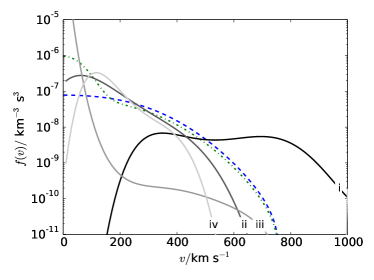
Figure 3: Example shapes for the directionally-averaged velocity distribution $f(v)$. These are labeled i-iv and are referred to in the text of Sec. IV, V and VI to explain the different regions of parameter space which can be fit to the data. For comparison, the Standard Halo Model (SHM) and the SHM with a dark disk (SHM+DD) are shown as dashed blue and dot-dashed green lines respectively.

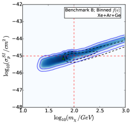
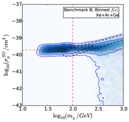
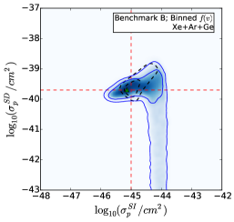
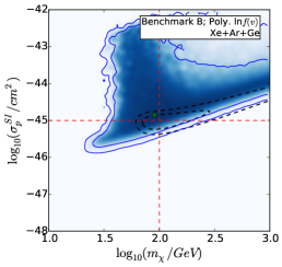
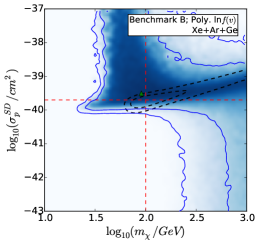
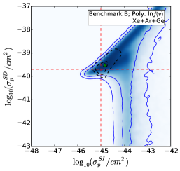
Figure 4: Same as Fig. 2 but for benchmark B.

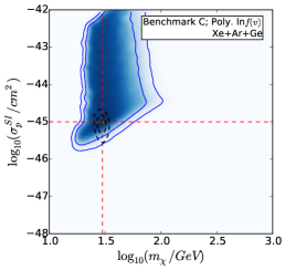
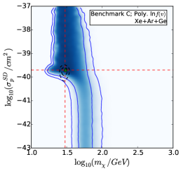
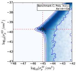
Figure 5: Same as Fig. 2 but for benchmark C.

IV.2 Benchmark B

Figure 4 shows the 2-dimensional profile likelihood distributions in the case of benchmark B, which has the same values of the particle physics parameters as benchmark A, but the input speed distribution includes a dark disk. The results for benchmark B with the speed distribution fixed to its input form (dashed black) are similar to those for benchmark A. However, the 95% confidence contours now extend up to large WIMP masses (left and central panels). When the WIMP mass is increased, the relative number of events in the xenon experiment can be too small. However, in benchmark B (unlike benchmark A) this is counteracted by the steep velocity integral at low speeds, due to the presence of the dark disk.

Again, when we allow the speed distribution to vary, the contours are significantly wider. In the case of the binned speed distribution, the likelihood peaks at around $m_{\chi}\approx 50\textrm{ GeV}$, compared to the input value of $100\textrm{ GeV}$. A possible bias in the WIMP mass when using the binned distribution has been noted previously Peter (2011); Kavanagh and Green (2012), although in this case the effect is relatively minor and the input value lies within the 68% contours. When the polynomial parametrisation is used, the best-fit point is closer to the input parameter values. However, there is a strong degeneracy between the mass and the cross sections, and consequently for both parameterisations the displacement of the best-fit point away from the input parameter values is much smaller than the uncertainties on the parameters.

A significant difference between the two parameterisations is that the contours for the polynomial parametrisation extend up to large values of $\sigma_{\mathrm{p}}^{\mathrm{SI}}$ and $\sigma_{\mathrm{p}}^{\mathrm{SD}}$ (this is most apparent in the lower-right panel of Fig. 4). This is a manifestation of the degeneracy described in Sec. I. Direct detection experiments do not probe the low-speed WIMP population. Thus, a velocity integral which is compatible with the input one in the region probed by the experiments but sharply increasing towards low speeds can still produce a good fit, provided that the cross section is also increased to give the correct total number of events. An example of such a distribution is shown in Fig. 3, labeled ‘iii’. These rapidly varying distributions are more easily accommodated in the polynomial parametrisation than in the binned one, which explains why the contours do not extend to large cross sections in that case (top row).

This region at large cross sections for the polynomial parameterisation did not appear in the case of benchmark A. This is because the parameter space describing the shape of the speed distribution is very large and distribution functions which rise rapidly at low $v$ do not make up a large fraction of the parameter space and, therefore, may not be well explored. In the case of benchmark B (which has a dark disk component), the input $f(v)$ is already increasing towards low speeds. This means that such rapidly rising distributions are better explored and this degeneracy becomes clear. The degeneracy up to high cross sections would become manifest for benchmark A if significantly more live points were used in the parameter scan. Therefore, the boundaries of the contours in Fig. 2 for benchmark A at large $\sigma_{\mathrm{p}}^{\mathrm{SI}}$ and $\sigma_{\mathrm{p}}^{\mathrm{SD}}$ should be considered as lower limits.

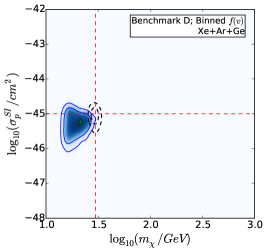
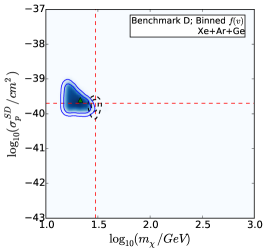
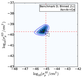
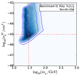
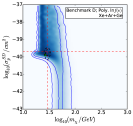
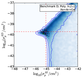
Figure 6: Same as Fig. 2 but for benchmark D.

IV.3 Benchmark C

Figure 5 shows the results for benchmark C, for which the mass is reduced to 30 GeV, with cross sections of $\sigma_{\mathrm{p}}^{\mathrm{SI}}$ = $10^{-45}\textrm{ cm}^{2}$ and $\sigma_{\mathrm{p}}^{\mathrm{SD}}$ = $2\times 10^{-40}\textrm{ cm}^{2}$ and a SHM $f(v)$. As for benchmarks A and B, using a fixed speed distribution (black dashed) leads to closed contours and tight constraints on the WIMP parameters and, with the binned parametrisation (top row), there again appears to be a slight bias towards lower WIMP masses, although the contours are not significantly widened. Indeed, for a binned $f(v)$, the reconstruction works quite well and all three quantities are determined with a good precision (approximately one order of magnitude for the cross sections and a factor of 2 for the WIMP mass). However, the results of the scan using the polynomial parametrisation (bottom row) are dramatically different. The 95% confidence contours now extend up to $m_{\chi}\approx 100\textrm{ GeV}$, owing to the wide range of functional forms which can be explored by this parametrisation. The degeneracy in the cross sections up to large values is even more pronounced than in the case of benchmark B. The lower input WIMP mass of benchmark C means that the region not covered by direct detection experiments extends up to $v\sim 200\textrm{ km s}^{-1}$, giving more freedom to the velocity integral to increase at low $v$.

For the polynomial parametrisation, the contours extend down to arbitrarily small values of $\sigma_{\mathrm{p}}^{\mathrm{SD}}$. As in the case of the higher mass benchmarks, explaining the data with only SI interactions requires a steeper velocity integral. For the low mass benchmarks, the fiducial spectrum is already relatively steep, requiring a velocity integral which is even steeper to give a good fit to the data at higher values of $m_{\chi}$. This is possible using the rapidly-varying polynomial parametrisation but not using the binned parametrisation, allowing the low $\sigma_{\mathrm{p}}^{\mathrm{SD}}$ region to enter the confidence contours only in the former case.

IV.4 Benchmark D

Finally, in Fig. 6 we show the results for benchmark D. These are very similar to those for benchmark C. This is because the contribution of the dark disk is predominantly below $v\sim 200\textrm{ km s}^{-1}$, and for a 30 GeV WIMP this is beneath the lowest speed probed by the direct detection experiments considered. The main difference with respect to benchmark C is the fact that now there is a very clear bias in the WIMP mass for the binned speed distribution. The reconstruction prefers low values of $m_{\chi}$ and the input parameter values are now outside the 95% contours.

In this section, we have presented the results of parameter reconstructions for $(m_{\chi},\sigma_{\mathrm{p}}^{\mathrm{SI}},\sigma_{\mathrm{p}}^{\mathrm{SD}})$ using data from multiple direct detection experiments only. As expected, when astrophysical uncertainties are neglected, the reconstruction of these parameters is very precise (apart from well known degeneracies between the WIMP mass and cross section). When $f(v)$ is allowed to vary in the fit, the confidence contours for the parameters are significantly widened. Using the 10-bin parametrisation, there is a clear bias in the WIMP mass for certain choices of benchmark parameters (in particular, benchmark D which has a light WIMP and a dark disk). This bias arises because bins of a fixed width in $v$ correspond to smaller bins in $E_{R}$ for smaller WIMP masses. This means that reducing the reconstructed WIMP mass allows a closer fit to the data, leading to the observed bias (see Ref. Kavanagh and Green (2012) for a detailed discussion).

The 6-polynomial parametrisation does not exhibit such a bias, but leads to even larger parameter uncertainties than for the binned parametrisation. Most notably, the confidence contours for the cross sections extend up to arbitrarily large values. Nonetheless, we obtain closed intervals for the WIMP mass when the input value is light (30 GeV, benchmarks C and D) relative to the mass of the detector nuclei, for both of the parameterisations of $f(v)$.

V Direct detection and IceCube data

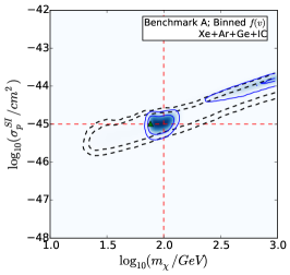
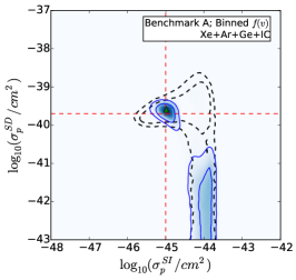
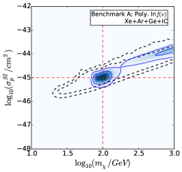
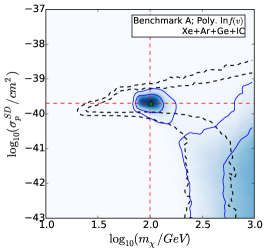
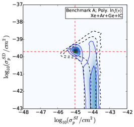
Figure 7: Same as Fig. 2 for benchmark A but using data from both direct detection and IceCube experiments. In this case, dashed black contours show the 68% and 95% confidence contours obtained using direct detection data only (i.e. they correspond to the blue contours of Fig. 2).

In this section, we present the results of scans performed using both direct detection and IceCube data.

V.1 Benchmark A

Figure 7 shows the 2-dimensional profile likelihood distributions in the case of benchmark A when IceCube data is included, in addition to the three direct detection experiments. The dashed black contours now correspond to the 68% and 95% confidence contours obtained using direct detection data only for comparison. The blue contours are with IceCube data and are considerably smaller than the dashed black ones.

When astrophysical uncertainties are included, the profile likelihood is multimodal. There is a small region of allowed parameter space around the input parameter values, and a second region at large masses, large SI and negligible SD cross sections. This is true for both parametrisations, with the only slight difference being that, for the polynomial parametrisation, the two regions are almost connected at the 95% confidence level. This is because the polynomial parametrisation can explore a wider range of shapes for the speed distribution, allowing the data to be fit reasonably well with a wider range of WIMP masses.

The strong degeneracy in the WIMP mass, which occurs when only direct detection data is used, has been substantially reduced with the inclusion of IceCube data. Low mass WIMPs are no longer viable as they cannot produce the observed number of events above the threshold of IceCube. As discussed in Sec. IV, at large masses two scenarios were possible with direct detection data only: a region at low $\sigma_{\mathrm{p}}^{\mathrm{SD}}$, where the observed events were explained in terms of SI interactions only, and a mixed SI/SD scenario (top right corner of all the panels of Fig. 2), with velocity integrals slightly steeper than the input one of the SHM. Including the information from IceCube eliminates this second possibility, as it produces too many neutrinos in IceCube. The number of neutrinos produced in IceCube could be reduced with a $f(v)$ which goes rapidly to zero below $\sim 200\,{\rm km\,s}^{-1}$. An example of such a distribution is shown in Fig. 3, labeled ‘iv’. However, the shape of the resulting velocity integral cannot be reconciled with the spectrum of direct detection events, especially in the xenon experiment.

With small $\sigma_{\mathrm{p}}^{\mathrm{SD}}$ and large $m_{\chi}$, good fits to the direct detection data are obtained by making the velocity integral even steeper and, since $\sigma_{\mathrm{p}}^{\mathrm{SD}}$ is small, the expected number of neutrinos is compatible with the number observed in IceCube. Therefore the region of parameter space at large WIMP masses and small $\sigma_{\mathrm{p}}^{\mathrm{SD}}$ is still allowed when IceCube data is added.

We can again compare to the work of Arina et al.  (in particular, the middle row of Fig. 3 of Ref. Arina et al. (2013)). Our accurate reconstruction of the WIMP mass matches that found in Ref. Arina et al. (2013) when direct detection and IceCube are combined. In contrast, we obtain significantly stronger constraints on the SI cross section. As previously stated, this is due to the fact that the present analysis uses an ensemble of different direct detection experiments. However, we note that here we have fully accounted for general uncertainties in the speed distribution and yet we can still obtain constraints similar to those of Arina et al.

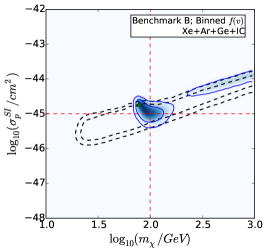
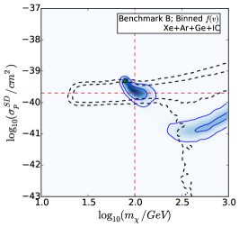
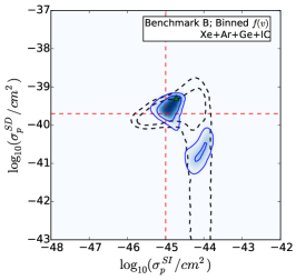
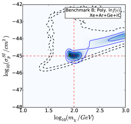
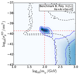
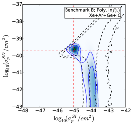
Figure 8: Same as Fig. 7 but for benchmark B.

V.2 Benchmark B

Figure 8 contains the same plots as Fig. 7, but for benchmark B, which has an additional contribution to the speed distribution from a dark disk. For both parametrisations, the results are similar to those for benchmark A. The only notable difference is that for the binned distribution (top row), the allowed region of parameter space at large masses is now bounded from below in $\sigma_{\mathrm{p}}^{\mathrm{SD}}$. In this region all the events in the direct detection experiments are due to SI interactions (and the velocity integral is quite steep) and the SD cross section is small enough not to overproduce neutrinos in IceCube. Decreasing $\sigma_{\mathrm{p}}^{\mathrm{SD}}$ further has no effect on the direct detection experiments, while underproducing the signal in IceCube. With the polynomial parameterisation it is possible to compensate for this underproduction of neutrinos by increasing the speed distribution below 50 – 80 ${\rm km\,s}^{-1}$, where it has no effect on the direct detection experiments. However this is not possible with the binned parameterisation, since the first bin extends up to 100 ${\rm km\,s}^{-1}$ and any change would also affect the number of events in xenon. This lower bound on the SD cross section for the binned parameterisation was not present for benchmark A as that benchmark only predicts 43.3 neutrinos (compared to the 242.9 of benchmark B). The smaller number of expected neutrinos means that benchmark A is less sensitive to changes in the number of neutrinos, and regions of parameter space with few neutrinos are still allowed.

Comparing the results with and without IceCube data (solid blue and dashed black contours respectively) using the polynomial parametrisation for benchmark B, we see that the regions of parameter space which extended up to large values of the cross sections are eliminated when IceCube data is included. This is most clear in the bottom right panel of Fig. 8, in which the contours no longer extend into the upper right hand corner. With direct detection data only, this region was allowed due to the possibility of having steeply rising velocity integrals for speeds which direct detection experiments could not probe. However the IceCube event rate is sensitive to these low speeds and such distributions would produce too many neutrino events.

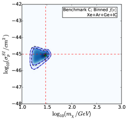
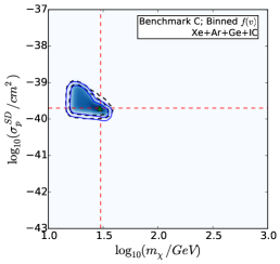
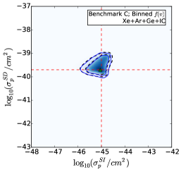
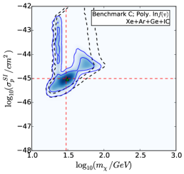
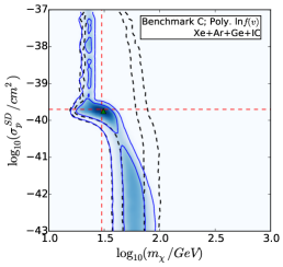
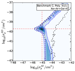
Figure 9: Same as Fig. 7 but for benchmark C.

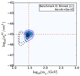
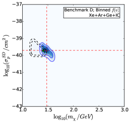
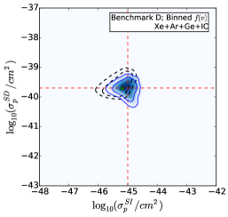
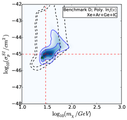
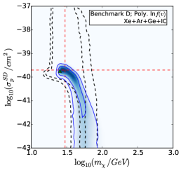
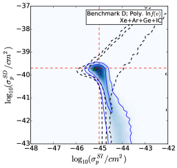
Figure 10: Same as Fig. 7 but for benchmark D.

V.3 Benchmark C

Figure 9 shows the same plots as Fig. 7, but for benchmark C, which has a smaller input WIMP mass. Using the binned parametrisation (top row), the confidence contours are not significantly changed from the case with direct detection only. This is because the number of signal events in IceCube is just 13, which is consistent with the observed background at just over $1\sigma$. As previously discussed, the binned distribution does not probe distribution functions which rise rapidly at low $v$. Because these are the only distribution functions which would be excluded by the small number of signal events, the addition of the IceCube data therefore has little impact on parameter reconstruction.

Using the polynomial parametrisation, the region at large $m_{\chi}$ where both SI and SD interactions are significant is now excluded. Similarly, a part of the parameter space at high cross section is now also excluded. As for the higher mass benchmarks, distributions which rise rapidly at low $v$ will overproduce events in IceCube and are therefore excluded. However, in contrast to the higher mass benchmarks, there remains a region which extends up to large cross sections at the 95% level. This region only occurs for WIMP masses below the sensitivity threshold of IceCube, $m_{\chi}=20\textrm{ GeV}$. Such low-mass WIMPs produce no signal events in IceCube and therefore any form of $f(v)$ can fit the IceCube data set (which is consistent with background at the $1\sigma$ level).

V.4 Benchmark D

Figure 10 show the same plots as Fig. 9, but for benchmark D, which has a contribution from a dark disk. This results in roughly three times more IceCube events than in benchmark C, which significantly improves parameter reconstruction. For the binned parametrisation, there is a noticeable shift in the contours to higher masses, so that they are more centered on the input mass value. In addition, the best-fit point lies closer to the input parameter values than in the case with only direct detection. WIMP masses below 20 GeV are excluded by IceCube data as they produce no signal events. Additionally, going to lower WIMP masses reduces the size of the bins in $E_{R}$ (which was the source of the previous bias), but requires a flatter form of $f(v)$ to fit the direct detection data. This flatter distribution results in a smaller solar capture rate and is therefore excluded as it produces too few IceCube events. The result is that the bias towards lower WIMP masses has been eliminated by the addition of IceCube data and the benchmark values now lie within the 68% contours.

Using the polynomial parametrisation, the high cross section regions of the parameter space are now entirely excluded, as the signal has a greater statistical significance than for benchmark C and cannot be explained by background alone. The shape of $f(v)$ is now reconstructed so as to neither overproduce or underproduce IceCube events. The 95% contours still extend down to small values of $\sigma_{\mathrm{p}}^{\mathrm{SD}}$. This is, as before, because the polynomial parametrisation encompasses steep velocity integrals, meaning that both direct detection and IceCube data can be explained with relatively small values $\sigma_{\mathrm{p}}^{\mathrm{SD}}$. This is not the case for the binned parameterisation.

In this Section we have found that for model-independent parametrisations of the WIMP speed distribution, using IceCube data in addition to direct detection data significantly reduces the size of the allowed particle physics parameter space. This extends the previous results of Ref. Arina et al. (2013) which used a fixed functional form for the speed distribution.

We find that with the addition of IceCube data, the bias in the reconstruction of the WIMP mass for the binned parametrisation is substantially reduced. The best-fit parameter values now lie close to the input values for all four benchmarks. A residual degeneracy between the SI and SD cross sections remains and, for some benchmarks, the signals can be explained in terms of SI interactions only. However, the large cross section degeneracy which arises for the polynomial parametrisation when using only direct detection data has been eliminated.

VI Reconstructing the speed distribution

In this section we present the reconstruction of the speed distribution using the polynomial and binned parametrisations.

VI.1 Polynomial parametrisation

In Fig. 11, we show the results for the polynomial parametrisation. The solid red lines indicate the best-fit functions, while the grey bands show the 68% and 95% confidence intervals. We note that the bands are obtained for each value of $v$ by profiling over all other values, as well as over the particle physics parameters. For reference, the SHM (dashed blue) and SHM+DD (dot-dashed green) distribution functions used in the benchmarks are also shown. For the plots in the left column only direct detection data are used in the likelihood, while for the right column IceCube data is also used.

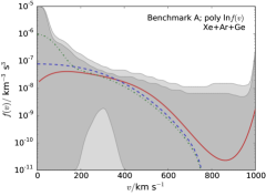
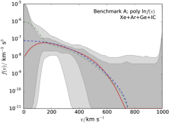
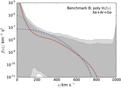
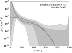
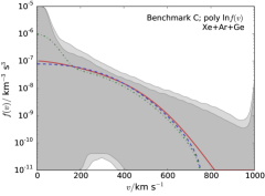
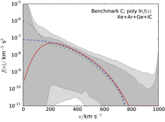
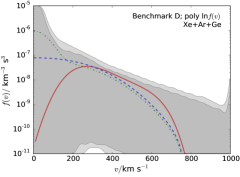
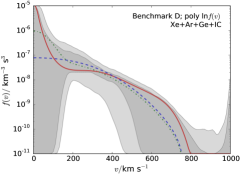
Figure 11: Reconstructions of the speed distribution using the polynomial parameterisation with 6 basis functions, using direct detection data only (left column) and using direct detection and IceCube data (right column). The four rows correspond to benchmarks A-D (from top to bottom). Benchmarks A and C (B and D) have the SHM (SHM+DD) as the input speed distribution. The dashed blue lines indicate the input SHM distribution while the dot-dashed green lines indicate the SHM+DD distribution. In each panel the solid red line shows the best fit, while the grey shaded bands show the 68% and 95% confidence intervals.

With only direct detection data, the uncertainties on the speed distribution are large. However, some features are apparent. For benchmark A, there is a light-grey-shaded region in the range $v\sim 200-400\,{\rm km\,s}^{-1}$ which does not lie within the 68% band. On the left side of this region, there is a contribution from flat speed distributions, such as the one labeled ‘i’ in Fig. 3, which provide a good fit to the data for light WIMPs. On the right side of this region, there is a contribution from steeper speed distributions, such as the one labeled ‘ii’ in Fig. 3, which provides a good fit for heavier WIMPs. Values of the speed distribution inside this light-grey region provide a poorer fit to the data as they underproduce low-energy events in xenon and/or high-energy events in argon.

This feature is not present in benchmark B because speed distributions which have low values above $v\sim 100\,{\rm km\,s}^{-1}$ and rise rapidly below this value are also allowed. These steeply-rising distributions are those corresponding to the regions of parameter space at very large $\sigma_{\mathrm{p}}^{\mathrm{SI}}$ and $\sigma_{\mathrm{p}}^{\mathrm{SD}}$ in Fig. 4.

Similar considerations, with the speed distribution decreasing below the speeds probed by xenon and above the speeds probed by argon, also explain the behaviour of the reconstruction of $f(v)$ for benchmarks C and D. However, for these benchmarks, the two regimes are closer to each other (since values of $m_{\chi}$ larger than 100 GeV are not allowed) and the different families of $f(v)$ overlap more.

When IceCube data is included (right panels), the constraints on $f(v)$ are significantly improved over some ranges of speed. The speed distributions which decrease below 200 ${\rm km\,s}^{-1}$ (as in the left panels) are eliminated, since the low $m_{\chi}$ values they correspond to are ruled out, as they would not produce neutrino events in IceCube. The IceCube data also disfavours the distributions which rise steeply below $v\sim 400\,{\rm km\,s}^{-1}$ which correspond to large values of both $\sigma_{\mathrm{p}}^{\mathrm{SI}}$ and $\sigma_{\mathrm{p}}^{\mathrm{SD}}$ (especially for benchmarks B, C and D). The net effect is that there is a range of speeds (around 200 ${\rm km\,s}^{-1}$ for benchmarks A and B and around 300 ${\rm km\,s}^{-1}$ for benchmark D) where $f(v)$ can be reconstructed within a factor of $\sim 4$. These speeds are just above the direct detection thresholds, where the most information about the shape of the recoil energy spectrum is available. At high speeds, $v>600\,{\rm km\,s}^{-1}$, the uncertainties remain large, as the direct detection experiments have no sensitivity to the shape of $f(v)$ above $E_{\textrm{max}}$. Finally, we note that the small number of IceCube signal events in benchmark C results in only a slight improvement in the bounds on $f(v)$.

Within the range of speeds where $f(v)$ is reconstructed well, the best-fit shape for benchmarks B and D (SHM+DD) is clearly steeper than for benchmarks A and C (SHM); the reconstruction has correctly recovered the rapidly rising dark disk contribution at low speeds.

We would now like to determine whether or not it is possible to exclude any particular form for the speed distribution using the mock data. The bands in Fig. 11 are calculated from the 1-dimensional profile likelihood separately at each value of $v$. However, the uncertainties at different values of $v$ are strongly correlated, due to the normalisation of $f(v)$. This means that not all shapes falling within the 68% band are consistent with the data at the 68% level. However, if a speed distribution falls outside the 68% band at some value of $v$, it can be rejected with at least 68% confidence.

A more powerful approach is to determine whether the data prefer a particular distribution over another. We focus on benchmark D, which has an input speed distribution with a dark disk and a low $m_{\chi}$, which allows a more accurate reconstruction of the speed distribution as discussed above. We compare the relative log-likelihoods of the best-fit point using the polynomial parametrisation with the best-fit assuming a fixed SHM distribution. In order to meaningfully compare the log-likelihoods of the two best-fit points, the two scans must be performed on parameter spaces that are nested one inside the other. Therefore, we must determine the combination of Chebyshev polynomials that provides a good fit to the SHM . We then fix the polynomial coefficients to the values obtained from this fit and perform a parameter scan over the remaining particle physics parameters. The best fit for the full $\ln f(v)$ parametrisation has a slightly higher log-likelihood value than the best fit when the coefficients are fixed to the SHM values. The relative log-likelihood between the two models corresponds to a value of $\Delta\chi^{2}=2.48$. This is perhaps not surprising, as the significance of the IceCube signal is not very large ($<3\sigma$), and it is this data which distinguishes the two distributions. For 5 degrees of freedom (the 5 free polynomial coefficients in the full parametrisation), the significance of this result is below the $1\sigma$ level and we therefore cannot reject the SHM speed distribution. However, this method allows us to make robust statements about the different speed distributions and may, with greater statistics, allow us to distinguish between them.

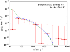
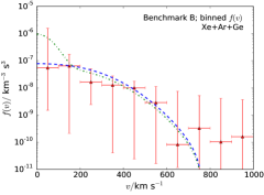
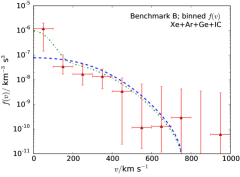
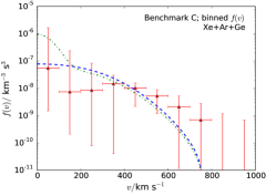
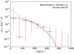
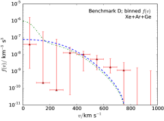
Figure 12: Same as Fig. 11 but for the binned parametrisation. The red triangles correspond to the best-fit point, while the red bars indicate the 68% confidence limits.

VI.2 Binned parametrisation

In Fig. 12, we show the speed distributions reconstructed using the binned parametrisation. The red triangles show the best-fit bin heights, while the error bars indicate the 68% confidence limits. As for the polynomial parametrisation, the error bar on each bin is obtained by profiling over all other parameters in the scan.

With only direct detection data, the uncertainties on the bin heights are large, with some of the 68% limits extending down to below $10^{-10}\textrm{ km}^{-3}\textrm{ s}^{3}$. In certain bins, however, the constraints are much stronger, with the bin heights constrained within a factor of roughly 5. For benchmarks C and D, $f(v)$ is reconstructed with better precision for large speeds (500 – 700 $\textrm{ km s}^{-1}$) than for the polynomial parameterisation. This is because very large $\sigma_{\mathrm{p}}^{\mathrm{SI}}$ and $\sigma_{\mathrm{p}}^{\mathrm{SD}}$ are not allowed with the binned parameterisation (see Figs. 5 and 6 and the discussion in Sec. IV). There is, however, mild tension with the input speed distribution for benchmark D (bottom left panel). In the range 500 – 700 $\textrm{ km s}^{-1}$, the reconstruction appears to overestimate the bin heights, resulting in a flatter shape for $f(v)$ than the input form. In this case, the reconstructed WIMP mass was lower than the input value. As discussed in Ref. Kavanagh and Green (2012), this is because reducing the WIMP mass reduces the size of the bins when converting to energy space, which leads to a better fit to the data. When the WIMP mass is decreased, the velocity integral needs to become less steep in order to counterbalance the steepening of the spectrum. The increased WIMP population in the range 500 – 700 $\textrm{ km s}^{-1}$ is then balanced by a depleted $f(v)$ at lower speeds in order to maintain the overall normalisation to unity. This results in very low bin heights in the range 100 – 200 $\textrm{ km s}^{-1}$.

As in the case of the polynomial parameterisation (Fig. 11), without IceCube data the reconstructed speed distributions for the pairs of benchmarks with and without a dark disk (A & B and C & D) are almost indistinguishable, as the direct detection experiments have little sensitivity at low speeds where they differ. When IceCube data is added, benchmarks B and D, which have a dark disk, show a clear spike in the lowest bin, which is not present for benchmarks A and C. We also note that the best-fit bin heights now trace the input speed distributions closely. As for the polynomial parameterisation, the uncertainties are smallest for speeds close to the direct detection thresholds (0 – 300 $\textrm{ km s}^{-1}$ for benchmarks A and B and 200 – 500 $\textrm{ km s}^{-1}$ for the lighter benchmarks C and D).

We note that a likelihood comparison between the binned distribution and some fixed $f(v)$ such as the SHM (as was performed for the polynomial parametrisation) may not be appropriate. This is because the 10-bin distribution does not provide as close an approximation to the shape of the SHM. Thus, such a likelihood comparison would not necessarily be meaningful.

VII Discussion

In Sec. IV, we examined the reconstruction of the WIMP mass and cross sections with binned and polynomial parametrisations of the speed distribution, using mock data from direct detection experiments only. As found in Refs. Peter (2011); Kavanagh and Green (2012, 2013); Kavanagh (2013), with the binned parametrisation there can be a bias in the WIMP mass. We also saw that there is a strong degeneracy between the SI and SD cross sections and the shape of the speed distribution when using only direct detection data. In particular, large cross sections can be accommodated by increasing the fraction of the WIMP population which lies below the direct detection energy thresholds. Even though this degeneracy was only apparent when using the polynomial $\ln f(v)$ parametrisation, it will affect all methods which make no astrophysical assumptions. The binned parametrisation of the speed distribution (top rows of Figs. 2, 4, 5 and 6) appears to lead to closed contours for the particle physics parameters. However, in the left column of Fig. 12, we demonstrate that this parametrisation is insensitive to the presence of a dark disk at low speeds, and it is this lack of sensitivity that leads to the spurious upper limits on the cross sections.

With the inclusion of IceCube data in Sec. V, the situation is significantly improved. The degeneracy to large cross sections is eliminated for all four of the benchmarks that we consider. The sensitivity of Solar capture to the low-speed WIMP population allows us to exclude the region of parameter space with large WIMP mass and large SI and SD cross sections, as it overproduces neutrino events at IceCube. The low mass region is also much more tightly constrained as if the mass is too small too few neutrinos are seen in IceCube. As seen in the top rows of Figs. 7, 8, and 10, the inclusion of IceCube data removes the bias in the reconstruction of the WIMP mass which occurs for the binned parameterisation with direct detection data only .

Some degeneracy still remains. In particular, it is possible to reduce the SD cross section significantly and compensate by increasing the SI contribution if, at the same time, the velocity integral is also made steeper at low speeds. It is possible to define an effective cross section, $\sigma_{\textrm{eff}}$, which incorporates both cross sections and controls the overall event rate. Due to the different response of each detector to SI and SD couplings, each experiment (including IceCube) will have a different $\sigma_{\textrm{eff}}$. Here, for simplicity, we focus on the case of a germanium detector for which

$$\sigma_{\textrm{eff}}=\sum_{i}f_{i}A_{i}^{2}\sigma_{\mathrm{p}}^{\mathrm{SI}}+f_{73}\frac{16\pi}{3}\frac{\sigma_{\mathrm{p}}^{\mathrm{SD}}}{2J+1}S_{00}(0)\,,$$ (35)

where $f_{i}$ and $A_{i}$ are the mass fraction and mass number of isotope $i$. Figure 13 shows the profile likelihood for $\sigma_{\textrm{eff}}$ with and without IceCube data (as solid and dashed lines respectively) for benchmark D, obtained using the polynomial parametrisation. Without IceCube data there is only a lower limit on $\sigma_{\textrm{eff}}$, below which there are too few events produced in the detector. For larger values of $\sigma_{\textrm{eff}}$, the profile likelihood is almost completely flat with an uncertainty of roughly three orders of magnitude. Including IceCube data, the profile likelihood becomes sharply peaked, with the value of $\sigma_{\textrm{eff}}$ constrained to within a factor of four at the 68% level. Clearly, the inclusion of IceCube data means that we can now reconstruct the value of the effective cross section, rather than only placing a lower limit.

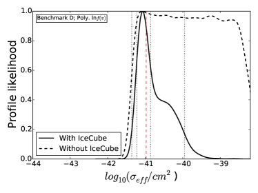
Figure 13: Profile likelihood for the effective cross section of germanium, $\sigma_{\textrm{eff}}$, (defined in Eq. (35)) for benchmark D, obtained using the polynomial parametrisation with and without IceCube data (solid and dashed black lines respectively). The vertical red dashed line corresponds to the input value for this benchmark while the vertical dotted black lines correspond to the 68% and 95% confidence intervals for the case with IceCube data.

The residual degeneracy between the SI and SD cross sections could be broken by the inclusion of an additional direct detection experiment using a nuclear element that is sensitive mainly to SD interactions Cerdeño et al. (2013); Cerdeno et al. (2014). This approach is currently taken by the COUPP and ROSEBUD collaborations Behnke et al. (2008); Coron et al. (2011) and is also proposed for the EURECA experiment Kraus et al. (2011).

As in Ref. Arina et al. (2013), the conclusions we draw apply even in the absence of a significant signal at IceCube, provided the WIMP is not too light. In benchmark C, the number of signal events is just 13, which is consistent with the observed background at just over $1\sigma$. Even with a signal of such low significance, we can still break the degeneracy between the cross section and $f(v)$, as explained above. However if the WIMP mass is smaller than the IceCube detection threshold, no neutrino events will be produced, regardless of the scattering cross sections and speed distribution. There is therefore no improvement in the reconstruction of the WIMP mass and the cross section degeneracy remains.

In Sec. IV we demonstrated that the binned speed parametrisation is not suitable when only direct detection data is used, as it may lead to a bias in the WIMP mass for certain benchmark parameters (see also Refs. Peter (2011); Kavanagh and Green (2012)). With the polynomial parametrisation, no such bias occurs. However, this parametrisation typically results in much larger parameter uncertainties than the binned one, including a significant degeneracy to large values of the cross sections. This is due to the fact that the polynomial parametrisation can explore a wider range of forms for $f(v)$, including distributions which are rapidly varying.

When IceCube data is included, the bias in the WIMP mass for the binned parametrisation is significantly reduced, as low WIMP masses underproduce events in IceCube. A binned parametrisation also leads to narrow parameter uncertainties (with closed contours in benchmarks B, C and D, see Figs. 8, 9 and 10) and tighter constraints on $f(v)$ than with the polynomial parametrisation. This is because the reconstruction using a polynomial decomposition encompasses qualitatively different, and larger, regions of the parameter space than that using the binned $f(v)$. For example, small values of $\sigma_{\mathrm{p}}^{\mathrm{SD}}$ are allowed at the 68% level in benchmarks B, C and D, only when the polynomial parametrisation is used. This is due to the fact that this parametrisation can encompass steep or rapidly varying distributions which, in these regions of the parameter space, are required to produce a good fit to the data.

It is not clear which speed parametrisation is optimal when direct detection and neutrino telescope data are combined. In this case, where the combined data are sensitive to the full range of WIMP speeds, the flexibility of the polynomial parametrisation may not be a benefit. In particular the rapidly varying shapes it probes may not be physically well motivated. For example, it is not clear how a $f(v)$ that is rapidly varying or rising at low speeds could arise in an equilibrium model of the Milky Way. If we are confident that the speed distribution does not contain sharp features, then the binned method, which is not sensitive to such features and produces tighter constraints on the particle physics parameters, is most suitable. However if we want to allow for a more general shape, with the possibility of sharp features, such as high density streams, the polynomial parametrisation is more appropriate. A pragmatic approach would be to use both parametrisations.

We note that we have made several assumptions in this work. We have neglected uncertainties in the SD form factors, which may lead to wider uncertainties on the particle physics parameters. Using the parametrisation in Ref. Cerdeno et al. (2012) would allow us to take this into account, and also compare the relative importance of nuclear and astrophysical uncertainties. Further simplifications include the assumptions of equilibrium between the capture and annihilation rates in the Sun, and the approximation that annihilations occur into a single channel. These uncertainties could be relaxed and incorporated as free parameters in the fit. In this paper, we focused on an idealized scenario which neglects these uncertainties in order to highlight the improvement in the determination of the WIMP particle physics and astrophysics parameters that can be achieved by combining data from a neutrino telescope with direct detection experiments. This is, however, a general phenomenon which can be exploited even for larger (and more realistic) parameter spaces.

VIII Conclusions

We have examined the effect of combining future direct detection and neutrino telescope data on reconstructions of the standard WIMP particle physics parameters ($m_{\chi}$, $\sigma_{\mathrm{p}}^{\mathrm{SI}}$ and $\sigma_{\mathrm{p}}^{\mathrm{SD}}$) and the local speed distribution $f(v)$. We account for uncertainties in the DM speed distribution by using two parametrisations: the binned parametrisation proposed in Ref. Peter (2011) and the polynomial $\ln f(v)$ parametrisation from Ref. Kavanagh and Green (2013). Direct detection data alone is only sensitive to speeds above a (WIMP-mass-dependent) minimum value. However the inclusion of neutrino telescope data allows the full range of WIMP speeds, down to zero, to be probed.

Our main conclusions can be summarised as follows:

• When only data from direct detection experiments are used, the polynomial speed parameterisation provides an unbiased measurement of the WIMP particle physics parameters. Even for benchmarks A and B, where the constraint contours for the particle physics parameters are not closed, the best-fit values are very close to the input values. This had previously been found for the case of SI-only interactions Kavanagh and Green (2013); Kavanagh (2013). Here we have shown that it also holds when the SI and SD cross sections are both non-zero. We have also confirmed the bias in the WIMP mass induced by the binned $f(v)$ parametrisation (as found in Ref. Kavanagh and Green (2012)).

• The inclusion of IceCube mock data significantly narrows the constraints on the WIMP mass, for both the binned and polynomial parametrisations. Most notably, the bias towards lower WIMP masses experienced with the binned parametrisation is removed.

• For the polynomial parametrisation of $f(v)$, including mock IceCube data eliminates a region of parameter space where the WIMP mass and scattering cross-sections are all large. With only the data from direct detection experiments the cross sections are degenerate with the shape of $f(v)$, so that increasing the velocity integral at low speeds (where the direct detection experiments are not sensitive), balances the effect of the large cross sections. Including the information from neutrino telescopes breaks this degeneracy, since these solutions overproduce neutrinos. The net effect is that with the addition of IceCube data upper limits can be placed on the strength of the SI and SD cross sections.

• With the combination of direct detection and neutrino data, the speed distribution is reconstructed to within an order of magnitude, over a range of speeds of $\sim 200\,{\rm km\,s}^{-1}$, for all four benchmarks considered, independently of the speed parametrisation employed. For the binned parametrisation the accuracy achieved is better (reduced to a factor of 3–4 for certain speeds), over a range as wide as $\sim 400\,{\rm km\,s}^{-1}$. The maximum sensitivity to the shape of $f(v)$ is achieved for speeds just above the threshold energies of the direct detection experiments. We have also demonstrated how these parametrisations can be used to make robust statistical comparisons between different speed distributions.

• Of the two parametrisations we have used, the binned method typically provides tighter constraints on both WIMP particle physics parameters and the shape of $f(v)$. The polynomial parametrisation allows a broader range of speed distributions to be explored, resulting in wider uncertainties on the reconstructed parameters. Some of these speed distributions are probably not physically well-motivated, for instance those that rise or fall steeply at low speeds. With data only from direct detection experiments, the polynomial parametrisation should be used to avoid the bias in the WIMP mass which can arise for the binned parametrisation. Given a future signal in both direct detection and neutrino telescope experiments, both parametrisation methods should be used, as a consistency check. However, if the speed distribution does not contain sharp features, the binned parametrisation will allow a reconstruction of the WIMP particle physics parameters, and also the speed distribution, that is reliable and more accurate.

• Even with the inclusion of IceCube data, it is not always possible to derive upper and lower limits on both the SI and SD cross sections. This is due to a residual degeneracy between the two. However, it is possible to define an effective cross section, $\sigma_{\textrm{eff}}$, that determines the total event rate and incorporates both the SI and SD cross sections. The combination of direct detection and neutrino telescope data allows both upper and lower limits to be placed on $\sigma_{\textrm{eff}}$.

We have shown that by combining direct detection and neutrino telescope data, unbiased reconstructions of not only the WIMP mass, but also the WIMP interaction cross sections, can be obtained without making restrictive (and potentially unjustified) assumptions about the WIMP speed distribution. Furthermore, the form of the speed distribution can also be reconstructed. This is possible because neutrino telescopes are sensitive to the entire low-speed WIMP population that lies beneath the thresholds of direct detection experiments. The addition of neutrino telescope data thus solves a problem that afflicts any strategy to recover the WIMP particle physics parameters and to probe $f(v)$ using direct detection data without making astrophysical assumptions. This demonstrates, and extends, the complementarity of the different techniques employed in the search for DM.

References

- Cerdeno and Green (2010) D. G. Cerdeno and A. M. Green, (2010), arXiv:1002.1912 [astro-ph.CO] .
- Strigari (2013) L. E. Strigari, Phys.Rept. 531, 1 (2013), arXiv:1211.7090 [astro-ph.CO] .
- Goodman and Witten (1985) M. W. Goodman and E. Witten, Phys.Rev. D31, 3059 (1985).
- Peter (2011) A. H. G. Peter, Phys. Rev. D 83, 125029 (2011), arXiv:1103.5145 .
- Feast and Whitelock (1997) M. Feast and P. Whitelock, Mon. Not. R. Astron. Soc. 291, 683 (1997), arXiv:astro-ph/9706293 .
- Bovy et al. (2012) J. Bovy, C. A. Prieto, T. C. Beers, D. Bizyaev, L. N. da Costa, et al., Astrophys.J. 759, 131 (2012), arXiv:1209.0759 [astro-ph.GA] .
- Smith et al. (2007) M. C. Smith, G. Ruchti, A. Helmi, R. Wyse, J. Fulbright, et al., Mon.Not.Roy.Astron.Soc. 379, 755 (2007), arXiv:astro-ph/0611671 [astro-ph] .
- Piffl et al. (2014) T. Piffl, C. Scannapieco, J. Binney, M. Steinmetz, R.-D. Scholz, et al., Astron.Astrophys. 562, A91 (2014), arXiv:1309.4293 [astro-ph.GA] .
- Evans et al. (2000) N. W. Evans, C. M. Carollo, and P. T. de Zeeuw, Mon. Not. R. Astron. Soc. 318, 1131 (2000), arXiv:astro-ph/0008156 .
- Widrow (2000) L. M. Widrow, Astrophys. J. Suppl. Ser. 131, 39 (2000).
- Bozorgnia et al. (2013) N. Bozorgnia, R. Catena, and T. Schwetz, JCAP 1312, 050 (2013), arXiv:1310.0468 [astro-ph.CO] .
- Bhattacharjee et al. (2013) P. Bhattacharjee, S. Chaudhury, S. Kundu, and S. Majumdar, Phys. Rev. D 87, 083525 (2013), arXiv:1210.2328 .
- Fornasa and Green (2013) M. Fornasa and A. M. Green, Phys. Rev. D 89 (2013), 10.1103/physrevd.89.063531, arXiv:1311.5477 .
- Fairbairn and Schwetz (2009) M. Fairbairn and T. Schwetz, JCAP 0901, 037 (2009), arXiv:0808.0704 [hep-ph] .
- Vogelsberger et al. (2009) M. Vogelsberger, A. Helmi, V. Springel, S. D. M. White, J. Wang, C. S. Frenk, A. Jenkins, A. Ludlow, and J. F. Navarro, Mon. Not. R. Astron. Soc. 395, 797 (2009), arXiv:0812.0362 .
- Kuhlen et al. (2010) M. Kuhlen, N. Weiner, J. Diemand, P. Madau, B. Moore, D. Potter, J. Stadel, and M. Zemp, J. Cosmol. Astropart. Phys. 02, 030 (2010), arXiv:0912.2358 .
- Mao et al. (2012) Y.-Y. Mao, L. E. Strigari, R. H. Wechsler, H.-Y. Wu, and O. Hahn, Astrophys. J. 764, 35 (2012), arXiv:1210.2721 .
- Kuhlen et al. (2012) M. Kuhlen, M. Lisanti, and D. N. Spergel, Phys. Rev. D 86, 063505 (2012), arXiv:1202.0007 .
- Read et al. (2009) J. I. Read, L. Mayer, A. M. Brooks, F. Governato, and G. Lake, Mon. Not. R. Astron. Soc. 397, 44 (2009), arXiv:0902.0009 .
- Read et al. (2010) J. I. Read, T. Bruch, L. Baudis, V. P. Debattista, O. Agertz, L. Mayer, A. M. Brooks, F. Governato, A. H. G. Peter, G. Lake, V. P. Debattista, and C. C. Popescu, AIP Conf. Proc. 1240, 391 (2010), arXiv:0901.2938 .
- Pillepich et al. (2014) A. Pillepich, M. Kuhlen, J. Guedes, and P. Madau, Astrophys. J. 784, 161+ (2014), arXiv:1308.1703 .
- Green (2012) A. M. Green, Mod.Phys.Lett. A27, 1230004 (2012), arXiv:1112.0524 [astro-ph.CO] .
- Green (2010) A. M. Green, JCAP 1010, 034 (2010), arXiv:1009.0916 [astro-ph.CO] .
- McCabe (2010) C. McCabe, Phys.Rev. D82, 023530 (2010), arXiv:1005.0579 [hep-ph] .
- Drees and Shan (2007) M. Drees and C.-L. Shan, JCAP 0706, 011 (2007), arXiv:astro-ph/0703651 [ASTRO-PH] .
- Strigari and Trotta (2009) L. E. Strigari and R. Trotta, JCAP 0911, 019 (2009), arXiv:0906.5361 [astro-ph.HE] .
- Fox et al. (2011) P. J. Fox, J. Liu, and N. Weiner, Phys.Rev. D83, 103514 (2011), arXiv:1011.1915 [hep-ph] .
- Peter (2010) A. H. Peter, Phys.Rev. D81, 087301 (2010), arXiv:0910.4765 [astro-ph.CO] .
- Feldstein and Kahlhoefer (2014) B. Feldstein and F. Kahlhoefer, J. Cosmol. Astropart. Physics 2014, 065 (2014), arXiv:1403.4606 .
- Peter et al. (2014) A. H. Peter, V. Gluscevic, A. M. Green, B. J. Kavanagh, and S. K. Lee, Phys.Dark Univ. 5-6, 45 (2014), arXiv:1310.7039 [astro-ph.CO] .
- Kavanagh and Green (2012) B. J. Kavanagh and A. M. Green, Phys. Rev. D 86, 065027 (2012), 1207.2039 .
- Kavanagh and Green (2013) B. J. Kavanagh and A. M. Green, Phys. Rev. Lett. 111 (2013), 10.1103/physrevlett.111.031302, arXiv:1303.6868 .
- Kavanagh (2013) B. J. Kavanagh, Phys. Rev. D 89, 085026 (2013), arXiv:1312.1852 .
- Press and Spergel (1985) W. H. Press and D. N. Spergel, Astrophys. J. 296, 679+ (1985).
- Silk et al. (1985) J. Silk, K. Olive, and M. Srednicki, Phys. Rev. Lett. 55, 257 (1985).
- Gaisser et al. (1986) T. Gaisser, G. Steigman, and S. Tilav, Phys. Rev. D 34, 2206 (1986).
- Krauss et al. (1986) L. Krauss, M. Srednicki, and F. Wilczek, Phys. Rev. D 33, 2079 (1986).
- Srednicki et al. (1987) M. Srednicki, K. A. Olive, and J. Silk, Nucl. Phys. B 279, 804 (1987).
- Griest and Seckel (1987) K. Griest and D. Seckel, Nucl. Phys. B 283, 681 (1987).
- (40) “http://icecube.wisc.edu/,” .
- Arina et al. (2013) C. Arina, G. Bertone, and H. Silverwood, Phys. Rev. D 88, 013002 (2013), arXiv:1304.5119 .
- Jungman et al. (1995) G. Jungman, M. Kamionkowski, and K. Griest, Phys. Rep. 267, 195 (1995), hep-ph/9506380 .
- Lee et al. (2013) S. K. Lee, M. Lisanti, and B. R. Safdi, JCAP 1311, 033 (2013), arXiv:1307.5323 [hep-ph] .
- McCabe (2014) C. McCabe, J. Cosmol. Astropart. Phys. 2014, 027 (2014), arXiv:1312.1355 .
- Freese et al. (1988) K. Freese, J. Frieman, and A. Gould, Phys. Rev. D 37, 3388 (1988).
- Helm (1956) R. Helm, Phys. Rev. 104, 1466 (1956).
- Lewin and Smith (1996) J. D. Lewin and P. F. Smith, Astropart. Phys. 6, 87 (1996).
- Fricke et al. (1995) G. Fricke, C. Bernhardt, K. Heilig, L. Schaller, L. Schellenberg, E. Shera, and C. Dejager, At. Data. Nucl. Data Tables 60, 177 (1995).
- Duda et al. (2007) G. Duda, A. Kemper, and P. Gondolo, J. Cosmol. Astropart. Phys. 2007, 012 (2007), hep-ph/0608035 .
- Co’ et al. (2012) G. Co’, V. De Donno, M. Anguiano, and A. M. Lallena, J. Cosmol. Astropart. Phys. 2012, 010+ (2012).
- Cannoni (2011) M. Cannoni, Phys. Rev. D 84, 095017 (2011), arXiv:1108.4337 .
- Ressell and Dean (1997) M. Ressell and D. Dean, Phys. Rev. C 56, 535 (1997), hep-ph/9702290 .
- Engel and Vogel (1989) J. Engel and P. Vogel, Phys. Rev. D 40, 3132 (1989).
- Iachello et al. (1991) F. Iachello, L. M. Krauss, and G. Maino, Phys. Lett. B 254, 220 (1991).
- Ellis and Flores (1988) J. Ellis and R. A. Flores, Nucl. Phys. B 307, 883 (1988).
- Cerdeno et al. (2012) D. G. Cerdeno, M. Fornasa, J.-H. Huh, and M. Peiro, Phys. Rev. D 87, 023512 (2012), arXiv:1208.6426 .
- Warburton et al. (1990) E. Warburton, J. Becker, and B. Brown, Physical Review C 41, 1147 (1990).
- Ressell et al. (1993) M. T. Ressell, M. B. Aufderheide, S. D. Bloom, K. Griest, G. J. Mathews, and D. A. Resler, Phys. Rev. D 48, 5519 (1993), hep-ph/9307228 .
- Dimitrov et al. (1995) V. Dimitrov, J. Engel, and S. Pittel, Phys. Rev. D 51, 291 (1995), hep-ph/9408246 .
- Menéndez et al. (2012) J. Menéndez, D. Gazit, and A. Schwenk, Phys. Rev. D 86, 103511 (2012), arXiv:1208.1094 .
- Cannoni (2013) M. Cannoni, Phys. Rev. D 87, 075014 (2013), arXiv:1211.6050 .
- Gould (1987) A. Gould, Astrophys. J. 321, 571+ (1987).
- Gould (1992) A. Gould, Astrophys. J. 388, 338+ (1992).
- Peter (2009) A. H. G. Peter, Phys. Rev. D 79, 103532 (2009), arXiv:0902.1347 .
- Aartsen et al. (2013a) M. Aartsen et al. (IceCube Collaboration), (2013a), arXiv:1309.7007 [astro-ph.HE] .
- Blennow et al. (2008) M. Blennow, J. Edsjo, and T. Ohlsson, J. Cosmol. Astropart. Phys. 2008, 021+ (2008), arXiv:0709.3898 .
- Baratella et al. (2014) P. Baratella, M. Cirelli, A. Hektor, J. Pata, M. Piibeleht, et al., JCAP 1403, 053 (2014), arXiv:1312.6408 [hep-ph] .
- Gondolo et al. (2004) P. Gondolo, J. Edsjo, P. Ullio, L. Bergstrom, M. Schelke, and E. A. Baltz, J. Cosmol. Astropart. Phys. 2004, 008 (2004), arXiv:astro-ph/0406204 .
- Gondolo et al. (2014) P. Gondolo, J. Edsjö, P. Ullio, L. Bergström, M. Schelke, E. Baltz, T. Bringmann, and G. Duda, http://www.darksusy.org (2014).
- Green (2007) A. M. Green, JCAP 0708, 022 (2007), arXiv:hep-ph/0703217 [hep-ph] .
- Pato et al. (2011) M. Pato, L. Baudis, G. Bertone, R. Ruiz de Austri, L. E. Strigari, et al., Phys.Rev. D83, 083505 (2011), arXiv:1012.3458 [astro-ph.CO] .
- Cerdeño et al. (2013) D. Cerdeño, C. Cuesta, M. Fornasa, E. García, C. Ginestra, et al., JCAP 1307, 028 (2013), arXiv:1304.1758 [hep-ph] .
- Cerdeno et al. (2014) D. Cerdeno, C. Cuesta, M. Fornasa, E. Garcia, C. Ginestra, et al., Int.J.Mod.Phys. A29, 1443009 (2014), arXiv:1403.3539 [astro-ph.IM] .
- Cowan et al. (2013) G. Cowan, K. Cranmer, E. Gross, and O. Vitells, Eur. Phys. J. C 71, 1 (2013), arXiv:1007.1727 .
- Strege et al. (2012) C. Strege, R. Trotta, G. Bertone, A. H. Peter, and P. Scott, Phys.Rev. D86, 023507 (2012), arXiv:1201.3631 [hep-ph] .
- Apr (2010) XENON1T at LNGS: Proposal April 2010, www.bo.infn.it/xenon/docs/xe1t_proposal_v2.pdf (2010).
- Bau (2013) SuperCDMS update: www.fnal.gov/directorate/program_planning/all_experimenters_meetings/special_reports/Bauer_supercdms_status_02_04_13.pdf (2013).
- Grandi (2005) L. Grandi, WARP: an argon double phase technique for Dark Matter search, Ph.D. thesis, Department of Nuclear and Theoretical Physics, University of Pavia (2005).
- Danninger and Strahler (2011) M. Danninger and E. Strahler, Proceedings of the 32nd ICRC, Beijing 5, 141 (2011).
- Silverwood et al. (2013) H. Silverwood, P. Scott, M. Danninger, C. Savage, J. Edsjö, J. Adams, A. M. Brown, and K. Hultqvist, J. Cosmol. Astropart. Phys. 03, 027 (2013), arXiv:1210.0844 .
- Scott et al. (2012) P. Scott et al. (IceCube Collaboration), JCAP 1211, 057 (2012), arXiv:1207.0810 [hep-ph] .
- Abbasi et al. (2009) R. Abbasi et al. (ICECUBE Collaboration), Phys.Rev.Lett. 102, 201302 (2009), arXiv:0902.2460 [astro-ph.CO] .
- Akerib et al. (2014) D. Akerib et al. (LUX Collaboration), Phys.Rev.Lett. 112, 091303 (2014), arXiv:1310.8214 [astro-ph.CO] .
- Aprile et al. (2013) E. Aprile et al. (XENON100 Collaboration), Phys.Rev.Lett. 111, 021301 (2013), arXiv:1301.6620 [astro-ph.CO] .
- Aartsen et al. (2013b) M. Aartsen et al. (IceCube collaboration), Phys.Rev.Lett. 110, 131302 (2013b), arXiv:1212.4097 [astro-ph.HE] .
- Cirelli et al. (2011) M. Cirelli, G. Corcella, A. Hektor, G. Hutsi, M. Kadastik, et al., JCAP 1103, 051 (2011), arXiv:1012.4515 [hep-ph] .
- Roszkowski et al. (2015) L. Roszkowski, E. M. Sessolo, and A. J. Williams, JHEP 1502, 014 (2015), arXiv:1411.5214 [hep-ph] .
- Schönrich (2012) R. Schönrich, Mon. Not. R. Astron. Soc. 427, 274 (2012), arXiv:1207.3079 .
- Bruch et al. (2009) T. Bruch, J. Read, L. Baudis, and G. Lake, Astrophys.J. 696, 920 (2009), arXiv:0804.2896 [astro-ph] .
- Choi et al. (2014) K. Choi, C. Rott, and Y. Itow, JCAP 1405, 049 (2014), arXiv:1312.0273 [astro-ph.HE] .
- Catena and Ullio (2010) R. Catena and P. Ullio, J. Cosmol. Astropart. Phys. 2010, 004 (2010), arXiv:0907.0018 .
- Weber and de Boer (2010) M. Weber and W. de Boer, Astron. Astrophys. 509, A25+ (2010), arXiv:0910.4272 .
- Zhang et al. (2013) L. Zhang, H.-W. Rix, G. van de Ven, J. Bovy, C. Liu, and G. Zhao, Astrophys. J. 772, 108+ (2013), arXiv:1209.0256 .
- Nesti and Salucci (2013) F. Nesti and P. Salucci, J. Cosmol. Astropart. Phys. 07, 016 (2013), arXiv:1304.5127 .
- Read (2014) J. Read, J.Phys. G41, 063101 (2014), arXiv:1404.1938 [astro-ph.GA] .
- Gould (1991) A. Gould, Astrophys. J. 368, 610+ (1991).
- Sivertsson and Edsjo (2012) S. Sivertsson and J. Edsjo, Phys. Rev. D 85, 123514 (2012), arXiv:1201.1895 .
- Feroz and Hobson (2007) F. Feroz and M. P. Hobson, Mon. Not. R. Astron. Soc. 384, 449 (2007), arXiv:0704.3704 .
- Feroz et al. (2008) F. Feroz, M. P. Hobson, and M. Bridges, Mon. Not. R. Astron. Soc. 398, 1601 (2008), arXiv:0809.3437 .
- Feroz et al. (2013) F. Feroz, M. Hobson, E. Cameron, and A. Pettitt, (2013), arXiv:1306.2144 [astro-ph.IM] .
- Green (2008) A. M. Green, JCAP 0807, 005 (2008), arXiv:0805.1704 [hep-ph] .
- Behnke et al. (2008) E. Behnke et al. (COUPP Collaboration), Science 319, 933 (2008), arXiv:0804.2886 [astro-ph] .
- Coron et al. (2011) N. Coron, J. Gironnet, P. de Marcillac, M. Martinez, T. Redon, et al., PoS IDM2010, 054 (2011).
- Kraus et al. (2011) H. Kraus, E. Armengaud, C. Augier, M. Bauer, N. Bechtold, et al., PoS IDM2010, 109 (2011).