Chandrasekhar’s relation and the stellar rotation in the Kepler field

Abstract

According to the statistical law of large numbers, the expected mean of identically distributed random variables of a sample tends toward the actual mean as the sample increases. Under this law, it is possible to test the Chandrasekhar’s relation (CR), $\langle V\rangle=(\pi/4)^{-1}\langle V\!\sin\,i\rangle$, using a large amount of $V\!\sin\,i$ and $V$ data from different samples of similar stars. In this context, we conducted a statistical test to check the consistency of the CR in the Kepler field. In order to achieve this, we use three large samples of $V$ obtained from Kepler rotation periods and a homogeneous control sample of $V\!\sin\,i$ to overcome the scarcity of $V\!\sin\,i$ data for stars in the Kepler field. We used the bootstrap-resampling method to estimate the mean rotations ($\langle V\rangle$ and $\langle V\!\sin\,i\rangle$) and their corresponding confidence intervals for the stars segregated by effective temperature. Then, we compared the estimated means to check the consistency of CR, and analyzed the influence of the uncertainties in radii measurements, and possible selection effects. We found that the CR with $\langle\sin\,i\rangle=\pi/4$ is consistent with the behavior of the $\langle V\rangle$ as a function of $\langle V\!\sin\,i\rangle$ for stars from the Kepler field as there is a very good agreement between such a relation and the data.

1. Introduction

Studies on stellar rotation distribution are performed from either equatorial rotations, $V$, usually calculated from rotation period measurements, or projected axial rotations $V\!\sin\,i$, measured from the spectral line profile broadening. When measurements of both $V$ and $V\!\sin\,i$ are available, one can fairly derive the inclination angle of the rotational axis to the line of sight. This makes it possible to determine the distribution of the inclination angles of the stars and hence the mean inclination angles of the rotational axes. In turn, the distribution of the inclination angles can provide evidence on the orientation of the rotational axes of a stellar population, and then determine whether or not these axes are randomly oriented.

The lack of observational evidence (Struve, 1945; Abt, 2001; Jackson & Jeffries, 2010), in addition to the scarce works pointing to a possible deviation from randomness (eg., Vink et al., 2005; Soares & Silva, 2011), which leads to a modification of the assumption of the randomness for the orientation of the stellar rotational axes, corroborate the frequency function of the inclination angles of the rotational axes with respect to the line of sight as $\sin\,i$ (cf. van Dien, 1948; Chandrasekhar & Münch, 1950). A consequence of the assumption of the randomness is the widespread relation between the mean rotational velocities obtained by Chandrasekhar & Münch (1950): $\langle V\rangle=(\pi/4)^{-1}\langle V\!\sin\,i\rangle$.

It is worth mentioning that regardless of what the frequency function of the inclination angles is, it is always possible to obtain the relation $\langle V\!\sin\,i\rangle=\langle V\rangle\langle\sin\,i\rangle$, by assuming that the mean $V$ and $\sin\,i$ are independent of each other. In fact, Chandrasekhar & Münch (1950) warned of the possibility that the inclination angle can have a frequency function other than $\sin\,i$ and that relation between the mean averages remains valid. Much has been released by using the Chandrasekhar’s ralation (CR), though a few works have been achieved to verify the validity of the frequency function $\sin\,i$ and the constant $\pi/4$ (eg., Abt, 2001; Jackson & Jeffries, 2010; Soares & Silva, 2011). Here we should mention Bernacca (1970) who stated that, when considering the rotation break-up limit, the inclination angle $i$ have a frequency function other than $\sin\,i$.

Nowadays, new instruments and telescopes, such as Kepler (Koch et al., 2010) and CoRoT (Baglin, 2006), can provide high-precision photometry for measurements of $V$ as much as $V\!\sin\,i$ to make possible statistical tests to investigate the inclination angle distribution to determine its true frequency function. Motivated by the plenty of observational data stemmed from these new telescopes, we carried out the present work. Aiming to advance discussions about the validity of the average $\langle\sin\,i\rangle=\pi/4$, this work aimed to estimate the mean inclination angles of rotational axes for field dwarf stars while checking the CR for the stars in the Kepler field.

2. Work sample

The complete work sample consists of one control sample of $V\!\sin\,i$ measurements and three samples of rotation period data for single main-sequence field stars with effective temperature, $T_{\rm eff}$, between 4 300 and 7 000 K (see Section 2.3). The control sample, hereafter N04, is from the magnitude-complete and kinematically unbiased sample of stars released by Nordström et al. (2004). The rotation periods, $P_{\rm rot}$, were determined in three studies using light curves (LC) from the Kepler mission archive. The samples contain rotation periods that are referred to R13, N13, and M14. Next, we will describe the main characteristics of the samples and the methods used in their measurements. We refer the reader to the original sources for complete details.

2.1. Projected Equatorial Rotations

Measurements of $V\!\sin\,i$ were carried out with the CORAVEL spectrometer (Baranne et al., 1979; Benz & Mayor, 1981) using the calibration technique by Benz & Mayor (1984). Such a technique allows the separation of the observational signature of the rotation from the micro and macroturbulence, pressure, and Zeeman splitting, which permits measurements of $V\!\sin\,i$ for slow rotators with an accuracy of $1\,{\rm km\,s}^{-1}$. For high rotators, the shallow cross-correlation profiles decrease the accuracy of the $V\!\sin\,i$ measurements. Therefore, the $V\!\sin\,i$ values higher than $30\,{\rm km\,s}^{-1}$ are given with uncertainties of $5-10\,{\rm km\,s}^{-1}$. To compose the control sample, we selected all of the stars with $V\!\sin\,i$ data in Nordström et al. (2004), except the objects classified as binary or cluster stars (see also Holmberg et al., 2009). The control sample has 7 542 $V\!\sin\,i$ data.

2.2. Rotation Periods

The R13 sample is composed of 20,631 $P_{\rm rot}$ measured by Reinhold et al. (2013) using data in the Quarter 3 (Q3) processed with the PDC-MAP pipeline. The stars were selected according to the criteria $\log g>3.5$ and variability amplitude $R_{\rm{var}}\geq 0.003$. The parameter $R_{\rm{var}}$ was defined as the 5th and 95th percentile of normalize flux, with 4 h boxcar smoothed differential LC. To detect periods, they used the Generalized Lomb–Scargle periodogram (Zechmeister & Kürster, 2009) to LC in 2 h bins. To minimize the aliasing caused by active regions on opposite hemispheres of the star, they compared the first two periods from the global sine fit. When the difference between the first and second period was less than 5%, they selected the longer one as the stellar rotation period. Aiming to exclude the pulsators, they selected a lower limit period equal to 0.5 day. A 45 day upper limit for the period was also selected to avoid instrumental effects, visible on timescales of the Q3 duration. In addition, all the periods close to the orbital period of known binaries were excluded.

Rotation periods in M14 are from McQuillan et al. (2014), and have 27,631 stars. Those authors used the LC from Q3 to Q14, which were corrected for instrumental systematics using PDC-MAP. They used the $T_{\rm eff}$-$\log g$ and color-color cuts by Ciardi et al. (2011) to select only main-sequence stars. The rotation periods were obtained using the method described by McQuillan et al. (2013), which is based on the autocorrelation function (ACF) of the LC. Such a method consists of measuring the degree of self-similarity of the LCs over a range of lags. The repeated spot-crossing signatures lead to ACF peaks at lags corresponding to $P_{\rm rot}$ and their integer multiples, in the case of rotational modulation. The authors considered only periods between 0.2 and 70 days to avoid excess of false positives from pulsators, and long periods difficult to determine. In addition, they selected only late-F stars ($T_{\rm eff}\lesssim 6\,500$ K because they were interested in the stars with convective envelopes. The eclipsing binaries and Kepler Objects of Interest (KOIs) were removed when identified.

The N13 sample contains 10,426 stars with the rotation period measured by Nielsen et al. (2013). These authors used eight quarters, from Q2 to Q9, corrected with the PDC-MAP. They applied a Lomb–Scargle periodogram (Frandsen et al, 1995) to determine the rotation periods from the LC. In their study, only active stars with $\log(g)\geq 3.4$ were selected, and a periodogram peak at least four times the white noise, estimated using the root mean square (rms) of the time series. The rotation period was determined as the median of the stable periods over the quarters. With the objective to avoid pulsators, they selected only $P_{\rm rot}\geq 1$ day. An upper limit period was assumed as 30 days because their method depends on the stable periods and does not work for longer periods. The objects known as eclipsing binaries, and KOIs were excluded from the sample.

The median of the rotation periods segregated by interval of effective temperature for the samples R13, M14, and N13 are given in Table 1.

Table 1Main Parameters of the Stars Analyzed in this Work

$\cdots$		N04		R13					M14					N13
$T_{\rm eff}$	$R_{\rm est}$	$N$	$\langle V\!\sin\,i\rangle$	$N$	$\langle V\rangle$	$\langle\Omega\rangle$	$\tilde{R}_{\rm KIC}$	$\tilde{P}_{\rm rot}$	$N$	$\langle V\rangle$	$\langle\Omega\rangle$	$\tilde{R}_{\rm KIC}$	$\tilde{P}_{\rm rot}$	$N$	$\langle V\rangle$	$\langle\Omega\rangle$	$\tilde{R}_{\rm KIC}$	$\tilde{P}_{\rm rot}$
$4300-4600$	0.66	17	$3_{-0.8}^{+0.9}$	1962	$2.7_{-0.2}^{+0.2}$	$3.8_{-0.3}^{+0.3}$	0.68	19.8	2383	$2.7_{-0.3}^{+0.3}$	$3.8_{-0.4}^{+0.5}$	0.68	23.7	652	$3.5_{-0.3}^{+0.3}$	$4.8_{-0.4}^{+0.4}$	0.70	14.0
$4600-4800$	0.69	35	$2.4_{-0.6}^{+0.6}$	1205	$3.5_{-0.3}^{+0.4}$	$3.8_{-0.4}^{+0.4}$	0.75	19.8	1365	$3.4_{-0.4}^{+0.5}$	$3.6_{-0.5}^{+0.5}$	0.75	24.0	394	$4.8_{-0.5}^{+0.5}$	$4.9_{-0.5}^{+0.6}$	0.77	14.0
$4800-5000$	0.72	124	$2.7_{-0.4}^{+0.5}$	1731	$4.1_{-0.4}^{+0.4}$	$4.1_{-0.3}^{+0.3}$	0.91	19.6	1751	$3.8_{-0.5}^{+0.5}$	$4.2_{-0.5}^{+0.6}$	0.88	23.5	597	$5.8_{-0.7}^{+0.9}$	$5.5_{-0.5}^{+0.5}$	0.92	13.6
$5000-5200$	0.76	236	$2.8_{-0.4}^{+0.4}$	2197	$4.2_{-0.4}^{+0.4}$	$4.0_{-0.3}^{+0.3}$	0.90	19.1	2410	$4.1_{-0.5}^{+0.5}$	$4.2_{-0.4}^{+0.5}$	0.89	22.	772	$6.4_{-0.7}^{+0.8}$	$5.6_{-0.4}^{+0.4}$	0.91	13.1
$5200-5400$	0.81	300	$2.9_{-0.3}^{+0.3}$	2511	$4.8_{-0.4}^{+0}$	$4.8_{-0.3}^{+0.3}$	0.86	17.6	2804	$5.2_{-0.5}^{+0}$	$5.6_{-0.6}^{+0.6}$	0.86	20.3	1006	$5.8_{-0.4}^{+0}$	$5.7_{-0.3}^{+0.4}$	0.89	12.1
$5400-5600$	0.88	682	$3.3_{-0.3}^{+0.3}$	2842	$4.5_{-0.3}^{+0}$	$4.7_{-0.2}^{+0.3}$	0.87	16.2	3216	$5.2_{-0.6}^{+0}$	$5.5_{-0.4}^{+0.5}$	0.86	18.5	1129	$5.7_{-0.3}^{+0}$	$5.8_{-0.3}^{+0.3}$	0.87	11.6
$5600-5800$	0.96	1010	$3.6_{-0.2}^{+0.3}$	2552	$5.1_{-0.3}^{+0.4}$	$5.1_{-0.3}^{+0.3}$	0.87	15.3	3237	$6.0_{-0.6}^{+0.6}$	$6.2_{-0.6}^{+0.6}$	0.87	17.5	1228	$6.2_{-0.4}^{+0.4}$	$6.2_{-0.3}^{+0.3}$	0.88	11.0
$5800-6000$	1.05	1253	$5.4_{-0.3}^{+0.3}$	2107	$6.8_{-0.5}^{+0.5}$	$6.5_{-0.4}^{+0.4}$	0.93	12.1	2930	$7.2_{-0.6}^{+0.6}$	$6.9_{-0.5}^{+0.5}$	0.94	14.6	1138	$7.7_{-0.5}^{+0.6}$	$7.2_{-0.4}^{+0.4}$	0.95	9.9
$6000-6200$	1.14	1416	$9_{-0.4}^{+0.4}$	1817	$8.4_{-0.5}^{+0.5}$	$7.9_{-0.4}^{+0.4}$	0.99	9.7	3042	$9.3_{-0.7}^{+0.8}$	$8.4_{-0.6}^{+0.6}$	1.01	11.9	1318	$9.3_{-0.6}^{+0.6}$	$8.2_{-0.4}^{+0.5}$	1.01	9.1
$6200-6400$	1.24	1278	$14.7_{-0.6}^{+0.6}$	987	$13.9_{-1.1}^{+1.2}$	$12.0_{-0.8}^{+0.8}$	1.04	6.6	2300	$13.7_{-0.9}^{+1}$	$11.1_{-0.7}^{+0.7}$	1.08	8.5	966	$13.5_{-1}^{+1}$	$11.1_{-0.6}^{+0.6}$	1.06	7.0
$6400-6600$	1.34	739	$21.1_{-0.9}^{+0.9}$	405	$25.9_{-2.5}^{+2.5}$	$20.4_{-1.7}^{+1.8}$	1.19	3.5	1520	$23.1_{-1.5}^{+1.7}$	$17.7_{-1.0}^{+1.2}$	1.23	4.5	627	$20.9_{-1.4}^{+1.4}$	$16.0_{-1.0}^{+1.0}$	1.24	4.1
$6600-6800$	1.42	332	$43.2_{-2.9}^{+3}$	177	$44.5_{-5.9}^{+6.1}$	$32.2_{-3.5}^{+3.5}$	1.32	2.0	657	$34.4_{-2.7}^{+2.9}$	$24.2_{-1.8}^{+1.9}$	1.35	3.0	348	$28.6_{-2.4}^{+2.5}$	$20.2_{-1.4}^{+1.5}$	1.39	2.9
$6800-7000$	1.49	120	$51.5_{-5.1}^{+5.5}$	138	$69.4_{-6.8}^{+7.6}$	$46.7_{-4.6}^{+5.0}$	1.51	1.1	16	$43.6_{-25.6}^{+36.8}$	$23.0_{-12.8}^{+15.7}$	1.58	5.2	251	$38.8_{-3.3}^{+3.3}$	$24.5_{-1.9}^{+1.8}$	1.51	2.1

Note. — The errors in the mean rotations represent the bootstrapped 95% confidence interval of the mean. The effective temperature is give in kelvins, estimated and median radii are given in $\,R_{\sun}$, mean rotations $\langle V\!\sin\,i\rangle$, and $\langle V\rangle$ are given in $\,{\rm km\,s}^{-1}$, $\langle\Omega\rangle$ is given in s^-1, and the median rotation period is given in days. The first Column presents the effective temperature ranges. Second and third column the radii, $R_{\rm est}$, estimated in the middle of the $T_{\rm eff}$ range using the data give in Table 1B by Gray (1992). Third and forth columns present the number of rotators in the sample N04, and the mean rotations, $\langle V\!\sin\,i\rangle$. Next columns show the parameters for the samples R13, N13, and M14 as indicated. These columns show the number of rotators, the mean rotations $\langle V\rangle$, mean angular rotation, $\langle\Omega\rangle$, the median KIC radii, $\tilde{R}_{\rm KIC}$, and the median rotation periods, $\tilde{P}_{\rm rot}$, respectively

2.3. Effective Temperatures

Effective temperatures of the stars in the N04 sample were determined by Nordström et al. (2004) using the calibration by Alonso et al. (1996), and the dereddened color indices $b-y$, $c_{1}$, and $m_{1}$. These stars have $T_{\rm eff}$ in the range $4\,300$-$7\,000$ K. Such a range defined the temperature interval of the stellar samples analyzed in this paper. Adopting a homogeneous scale of effective temperature for the stars in the Kepler field prevents the introduction of systematic bias as a result of using $T_{\rm eff}$ from different studies. Accordingly, the effective temperature of the Kepler targets was determined according to the homogeneous effective temperature scale by Pinsonneault et al. (2012). These authors used the Sloan Digital Sky Survey griz filters, tied to the fundamental temperature scale, to revise $T_{\rm eff}$ in the Kepler Input Catalog (KIC). As a result, they found a mean shift of about 215 K toward higher temperatures relative to the KIC $T_{\rm eff}$. In the present work, a systematic shift to higher $T_{\rm eff}$ results in a systematic shift down in the mean rotations $\langle V\rangle$ due to the displacement of some lower rotators to the next $T_{\rm eff}$ bin.

3. Mean rotations and confidence-intervals

Stellar rotation is correlated with spectral type or, equivalently, with effective temperature (see Figure 2 in Slettebak, 1970). Thus, to minimize the bias due to the mix of spectral types in our results, we binned the samples into 200 K bins (except the first one, which has a bin width of 300 K). Such a bin is the minimum range allowing a reasonable amount of stars ($\gtrsim 20$) for performing the bootstrap resampling.

True equatorial rotations (in $\,{\rm km\,s}^{-1}$) were calculated using the equation $V=50.58R_{\rm KIC}P_{\rm rot}^{-1}$, where $R_{\rm KIC}$ is the KIC radius (in $\,R_{\sun}$), and $P_{\rm rot}$ given in days. The angular rotations were calculated from $P_{\rm rot}$ according to the equation $\Omega=VR_{\rm KIC}^{-1}=50.58P_{\rm rot}^{-1}$, where $P_{\rm rot}$ is given in days, and $\Omega$ given in s^-1. The mean rotations, and their 95% confidence intervals in each $T_{\rm eff}$ bin, were estimated using bootstrap resampling (Efron, 1987; Efron & Tibshirani, 1993). The bootstrap-resampling method consists of generating a large number of data sets, each with an equal amount of data randomly drawn from the original data (cf. Feigelson & Babu, 2012). The way by which we proceeded was as follows. First, we performed a set of 1 000 bootstrap replications of the mean rotation in the $T_{\rm eff}$ bin. The mean value of the distribution of these bootstrapped means was assumed to be the mean rotation in the $T_{\rm eff}$ bin. Then, we ranked the bootstrapped means, from the lower to the higher value, and took the 25th and the 975th means in the rank as the lower and upper limits of the confidence interval, respectively. The mean rotations and their confidence intervals in each $T_{\rm eff}$ bin are presented in Table 1.

4. Some assumptions and approximations

Before proceeding further, it is important to make clear our assumptions. These are only approximations of the reality, once we are neither dealing with unbiased samples, nor accounting for all the effects contributing to the observed signature of the rotation periods.

For determining exactly the mean $\langle\sin{i}\rangle$ from $\langle V\sin{i}\rangle/\langle V\rangle$ it is necessary to have the mean equatorial rotations and the mean projected rotational velocities, both from the same sample of stars. Unfortunately, it is very difficult to produce a significant sample of $V$ and $V\sin{i}$ measurements. Given that there is no privileged direction in the Galaxy for stellar rotation, or, in other words, any representative sample of $V$ or $V\sin{i}$ in any direction of the Galaxy should have similar behavior to another representative sample in a different direction, it is possible to estimate the mean $\langle\sin{i}\rangle$ from these representative samples. Since the sample is homogeneous and the data are independent of each other, the mean rotation for each sample should represent the mean stellar rotation in the Galaxy—according to the statistical law of large numbers which states that the sample mean converges to the distribution mean as the sample size increases. Thus, as the mean $\langle V\rangle$ (or $\langle V\sin{i}\rangle$) of a sample represents the $\langle V\rangle$ (or $\langle V\sin{i}\rangle$) in the Galaxy, it must also represent the mean of the same physical quantity of another significant sample of stars. Based on these considerations, we assumed that the mean $\langle V\sin{i}\rangle$ from N04 represents the mean $\langle V\sin{i}\rangle$ of the Kepler field samples, since the former represents the mean of the physical quantity of all the stars with $T_{\rm eff}$ in the considered temperature bin. Likewise, the mean $\langle V\rangle$ from the Kepler field samples—because of their significances (large number of stars)—must represent the mean $\langle V\rangle$ of the field stars whatever the direction of Galaxy; therefore, it also represents the mean $\langle V\rangle$ of the N04 sample.

We presumed that each bootstrapped confidence interval contains a value close to the mean rotation of the entire population of rotators with $T_{\rm eff}$ ranging in the considered temperature bin. This assumption is reasonable because, except in a very few cases, the $T_{\rm eff}$ bins contain a large amount ($\gtrsim 120$) of stars with approximately the same spectral type. In addition, according to the Bootstrap Central Limit Theorem (Singh, 1981), bootstrapped means tend to become closer to the population true mean as the number of bootstrap resampling increases. This is clearly only an approximation because, apart from the bias introduced by the methods in determining $P_{\rm rot}$ (or $V\!\sin\,i$), there are additional biases in the samples. For instance, the stars in KIC are biased to solar-type stars, as the Kepler targets were selected in order to maximize the probability of detecting a planetary transit around stars similar to the Sun in mass and $T_{\rm eff}$ (Brown et al., 2011; Reinhold et al., 2013, see Figure 1). In addition, there is not sufficient information to remove all the binary stars or multiple systems from the samples.

We assumed rigid body rotation. In fact, as outlined by Reinhold et al. (2013), $P_{\rm rot}$ results from active regions with different velocities manifesting themselves as a superposition of different periods in the LC. They analyzed the distributions of $P_{\rm rot}$ and another period ($P^{\prime}$), within 30% of $P_{\rm rot}$, and found out in the remaining sines of their LC’s that these distributions are similar, presenting mean values of $P_{\rm rot}=16.3\pm 10.1$ days, and $P^{\prime}=13.3\pm 7.3$ days. They also found that the difference between the angular velocity at the stellar equator and at the pole increases weakly with the temperature in the range $3\,500$-$6\,000$ K, which is nearly the temperature range we are considering. According to these results, the differential rotation does not seem to strongly affect our conclusions.

We also assumed that the rotation period of the stellar chromosphere, which yields $P_{\rm rot}$, is equal to the rotation period of the photosphere, which yields $V\!\sin\,i$. This assumption is concerned with the problem in determining $\langle V\rangle$ from $\langle V\!\sin\,i\rangle$, highlighted by Soderblom (1985). As this author pointed out, it is likely that the stellar chromosphere rotates more rapidly than the photosphere as occur on the Sun. Furthermore, Soderblom (1985) drew attention to the fact that the problem of the spatial orientation of the rotation axes had two parts. First, the angle $i$, between the rotational axis and the line of sight, and second, the position angle of that axis on the plane of the sky. In this respect, we make clear that we are concerned only with the first part.

Finally, we take for granted that $V$ and $\sin\,i$ are independent variables, allowing us to equate their means as $\langle V\!\sin\,i\rangle=\langle V\rangle\langle\sin\,i\rangle$.

5. Results and discussion

Samples R13, M14, and N13 are very different from each other because the original samples have different selection criteria and methods in measuring $P_{\rm rot}$. About 70% of the objects in M14 are not in N13. More than 37% of the objects in the M14 sample are not in the R13 sample, and around 23% of the stars in the N13 sample do not belong to the R13 sample. The left panels of Figure 1 present the distribution of $P_{\rm rot}$ as a function of the $\bv$ color index, estimated using a calibration between $T_{\rm eff}$ and $\bv$ obtained from the data give in Table 1B by Gray (1992). The right panels shows the kernel density estimates of $P_{\rm rot}$. Although low and high rotators are present at all temperatures, it seems to be clear that there is a tendency for increasing rotation period with decreasing temperature, as predicted by the magnetic braking theory (Schatzma, 1962). There is a peak of probability around $P_{\rm rot}=12$ days, which for a star with radius $\sim 1\,R_{\sun}$ corresponds to a rotation of $V\sim 4\,{\rm km\,s}^{-1}$. A similar peak is observed in the distribution of $V\!\sin\,i$ in Figure 4 by Nordström et al. (2004), where we see a peak at $V\!\sin\,i\sim 3$-$4\,{\rm km\,s}^{-1}$. The periods in the R13 sample are limited to 45 days; however, there are only a few rotators with higher periods, which we can also see in the middle panel, for M14. The M14 sample presents a few stars with $T_{\rm eff}\gtrsim 6\,800$ K, because the stars are restricted to spectral region late-F (McQuillan et al., 2014). We also observe that the N13 sample is strongly biased against long periods, as we can observe by the sharp decline in the probability density function for the longer periods. This is due a limitation of the method used by Nielsen et al. (2013), as mentioned in Section 2.2. Finally, the sample N13 presents a sharp fall in the probability density function for the shorter periods, as a result of their lower limit period of one day.

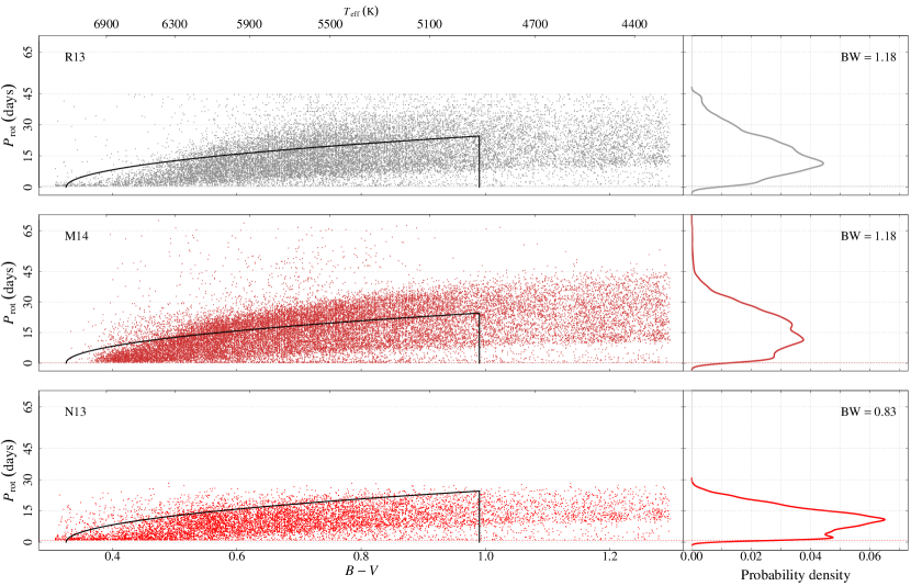
Figure 1.— Left panels display the distribution of rotation periods, $P_{\rm rot}$, as a function of the color-index, B V, for the sample R13, M14, and N13 as indicated. The regions limited by the curves in black enclose the stars with ages less than 2 Gyr and temperature in the range of 4 900-7 000 K. The top axis corresponds to the effective temperature. Right panels show the kernel density estimates for $P_{\rm rot}$ for the distribution in the same color. The smoothing bandwidth, BW, is indicated in each panel.

Figure 2 displays the distribution of $\langle V\rangle$ as a function of $\langle V\!\sin\,i\rangle$, in logarithmic scale. The $\langle V\!\sin\,i\rangle$ data from N04 spans over the horizontal axes, and the vertical axes correspond to $\langle V\rangle$ (left-side panels), or $\langle\Omega\rangle$ (right-side panels). First, we will analyze the left panels, then we will examine the panels on the right. In the left-side panels, the dashed line represent the CR model $\langle V\rangle=(\pi/4)^{-1}\langle V\!\sin\,i\rangle$, and the continuous line is the best-fit for the data. There is a very good agreement between the data from R13 and the CR model as can be observed comparing the CR model with the best fit line in panel (a). The best-fit line is given by $\langle V\rangle=1.2\langle V\!\sin\,i\rangle-0.2$, with the rms of the best fit ${\rm rms_{f}}=3.2\,{\rm km\,s}^{-1}$. The rms of the differences between $\langle V\rangle$ and the CR model is ${\rm rms_{CR}}=3.5\,{\rm km\,s}^{-1}$. The model is accepted with a 95% confidence level by six of 13 groups. Table 2 presents the median, minimum and maximum difference between $\langle V\rangle_{\rm CR}$ and $\langle V\rangle$, relatively to $\langle V\rangle$, for low, moderate, and high rotators, namely groups with $\langle V\!\sin\,i\rangle\lesssim 5\,{\rm km\,s}^{-1}$, $5\lesssim\langle V\!\sin\,i\rangle\lesssim 30\,{\rm km\,s}^{-1}$, and $V\!\sin\,i\gtrsim 30\,{\rm km\,s}^{-1}$, respectively. The largest median discrepancy occurs to the groups with moderate rotators. However, even such a discrepancy can be explained by considering the uncertainties in the KIC radii, as we will see below.

Table 2Relative Differences between the Mean Rotation Estimated with the CR Model, $\langle V\rangle_{\rm CR}$, and the Mean Rotation Calculated using $P_{\rm rot}$ and $R_{\rm KIC}$, $\langle V\rangle$.

Sample	$\langle V\!\sin\,i\rangle$	$\delta_{\rm min}$	$\delta_{\rm med}$	$\delta_{\rm max}$
	($\,{\rm km\,s}^{-1}$)	(%)	(%)	(%)
	$\lesssim 5$	9	12	36
R13	$\sim 5$-30	1	27	30
	$\gtrsim 30$	3	4	18
	$\lesssim 5$	6	15	28
M14	$\sim 5$-30	4	19	28
	$\gtrsim 30$	12	40	47
	$\lesssim 5$	6	29	36
N13	$\sim 5$-30	9	19	30
	$\gtrsim 30$	22	55	73

The agreement between the CR model and the data for the M14 sample is not as good as for the R13 sample. However, there is reasonable consistency $\langle V\rangle_{\rm CR}$ and $\langle V\rangle$ as we can see in panel (b). The best-fit line follows the equation $\langle V\rangle=0.8\langle V\!\sin\,i\rangle+2.3$, with ${\rm rms_{f}}=1.5\,{\rm km\,s}^{-1}$, and ${\rm rms_{CR}}=8.6\,{\rm km\,s}^{-1}$. According to the best-fit line, the groups with low rotators tend to present $\langle V\rangle>\langle V\rangle_{\rm CR}$. The groups with moderate and high rotators tend to have $\langle V\rangle<\langle V\rangle_{\rm CR}$, and there is even a group presenting $\langle V\!\sin\,i\rangle>\langle V\rangle$. A similar behavior is presented by the N13 sample, as we see in panel (e). The best-fit line for N13 data follows the equation $\langle V\rangle=0.7\langle V\!\sin\,i\rangle+3.8$, with ${\rm rms_{f}}=1.6\,{\rm km\,s}^{-1}$, and ${\rm rms_{CR}}=10.8\,{\rm km\,s}^{-1}$. The median relative differences between $\langle V\rangle$ and $\langle V\rangle_{\rm CR}$ for the samples M14 and N13, are shown given in Table 2. These discrepancies seem to be due primarily to two factors, the uncertainties in the KIC radii, and selection effects in the samples, as we will discuss next.

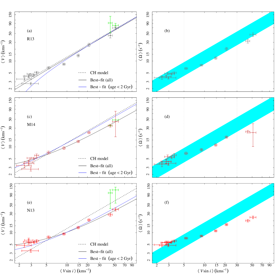
Figure 2.— Left-side panels show the mean true rotations as a function of the mean projected rotations. The error bars are bootstrapped 95% confidence intervals. The dashed line is the Chandrasekhar’s relation, the continuous black line is the best-fit line for the data, and the blue line is the best-fit line for the data of the subsample containing only stars with ages $<2$ Gyr and $4\,900\leqq T_{\rm eff}\leqq 7\,000$ K. The green dots represent the corrected means from the NPMLE (see the text), and their correspondent error bars are the 95% confidence bands of the NPMLE estimated through bootstrap resamples with 1000 replacements. The right-side panels present the mean true angular rotation as a function of the mean projected rotations. The cyan region corresponds to the mean angular rotation calculated from $\langle V\!\sin\,i\rangle$ by $\langle\Omega\rangle=(R\,\pi/4)^{-1}\langle V\!\sin\,i\rangle$, where radii $R$ span in a range from the minimum to the maximum median KIC radii, $\tilde{R}_{\rm KIC}$, given in Table 1. The axes are in logarithmic scale and the error bars represent the bootstrapped 95% (percentile) confidence interval for the means.

Radii from KIC were estimated from $\log(g)$ using a mass–radius relationship. They have uncertainties due to errors in photometry, degeneracies between stellar parameters and colors, as well as errors from stellar models (cf. Gaidos & Mann, 2013). Verner et al. (2011) compared KIC and astroseismic radii for 500 solar-type stars and found an underestimation bias of up to 50% for stars with $R_{\rm KIC}<2\,R_{\sun}$. Such a discrepancy is the result of the overestimated values of the KIC $\log(g)$. Analyzing uncertainties in the KIC radii of KOI stars, Gaidos & Mann (2013) found that K-type dwarfs have inaccuracies less than about 15%, while F- and many G-type stars have uncertainties that can be higher than 100%. We estimated the typical radii for the stars in our samples using the mean temperature of the stars in each $T_{\rm eff}$ bin considered (see Table 1), according to the calibration between $T_{\rm eff}$ and radii given in Table B1 by Gray (1992). The estimated radii, $R_{\rm est}$, as well as the median KIC radii, $\tilde{R}_{\rm KIC}$, is given in Table 1. Figure 3 shows that $\tilde{R}_{\rm KIC}$ are overestimated relatively to $R_{\rm est}$ for stars with $T_{\rm eff}\lesssim 5\,500$ K, and underestimated for stars with $T_{\rm eff}$ in the range $5\,500\lesssim T_{\rm eff}\lesssim 6\,900$ K. However, there is a reasonable agreement between $R_{\rm KIC}$ and $R_{\rm est}$, by considering the error bars. The mean relative difference between $R_{\rm KIC}$ and $R_{\rm est}$, relatively to $R_{\rm est}$, is around 10% for all the samples. The effect of an overestimation (or underestimation) of the median radius is a systematic proportional increase (or decrease) in $\langle V\rangle$. It is clear that $R_{\rm est}$ is a rough approximation of the central tendency of stellar radii in each $T_{\rm eff}$ interval. In fact, it does not consider many factors influencing the radius estimates, such as the stellar composition and evolution in the main sequence. The whole point of comparing $\tilde{R}_{\rm KIC}$ and $R_{\rm est}$ is to show that the lower and higher $\tilde{R}_{\rm KIC}$ presented in Table 1 are reasonable estimates of the radius variation limits for the stars in our samples, despite the large uncertainties in $R_{\rm KIC}$.

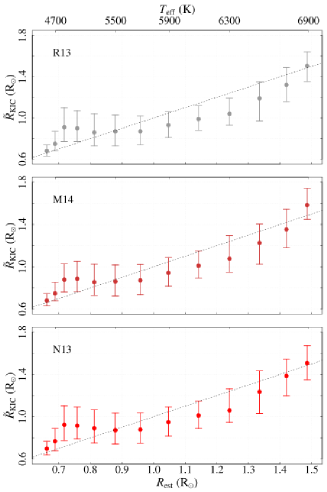
Figure 3.— Median KIC radii, $\tilde{R}_{\rm KIC}$, as a function of estimated typical radii, $R_{\rm est}$, for stars in each $T_{\rm eff}$ bin (see Table 1). The error bars are the first and third quartiles of the distribution of $R_{\rm KIC}$ in the $T_{\rm eff}$ bin. The black curve is the line of equality, and the top axis corresponds to the effective temperature.

In Figure 2 (panels (b), (d), and (f)), we present the behavior of $\langle\Omega\rangle$ as a function of $\langle V\!\sin\,i\rangle$. The cyan region corresponds to the angular rotations estimated from $\langle V\!\sin\,i\rangle$, according to the equation $\langle\Omega\rangle_{\rm Model}=(\pi/4)^{-1}R^{-1}\langle V\!\sin\,i\rangle$. For each sample, the parameter $R$ ranges from the minimum to the maximum $\tilde{R}_{\rm KIC}$ given in Table 1. Panel (b) reinforces the statement that there is a very good agreement between the behavior of the $\langle V\rangle$ as a function of $\langle V\!\sin\,i\rangle$ and the CR model. In fact, if we consider that the radii of the stars range approximately from the minimum to the maximum $\tilde{R}_{\rm KIC}$, we have that 12 in 13 groups support the CR model with a 95% confidence level. It is also worth noting that even a systematic decrease of $4\,{\rm km\,s}^{-1}$ in $V\!\sin\,i$ is sufficient to bring the outside group into the cyan region. Such a systematic shift down is reasonable because the $V\!\sin\,i$ data from N04 are biased to up ($5$-$10\,{\rm km\,s}^{-1}$) to values higher than $30\,{\rm km\,s}^{-1}$, as we mentioned in Section 2.1.

In the panel (d), we observe that 11 in 13 groups of stars present a behavior of $\langle\Omega\rangle$ with $\langle V\!\sin\,i\rangle$ consistent with the CR model. The groups outside the cyan area have $\langle V\!\sin\,i\rangle>30\,{\rm km\,s}^{-1}$. In order to make these two groups agree to the CR model, it is required that a systematic decrease of at least 13, and $23\,{\rm km\,s}^{-1}$ in $V\!\sin\,i$, or equivalently, a systematic decrease of about 30, and 45% in $P_{\rm rot}$. Panel (f) shows that the groups from the N13 sample with $V\!\sin\,i\gtrsim 15\,{\rm km\,s}^{-1}$ seem to rule out the model. For the groups with $15\lesssim\langle V\!\sin\,i\rangle<30\,{\rm km\,s}^{-1}$, a systematic shift down to about $2\,{\rm km\,s}^{-1}$ in $V\!\sin\,i$, or an increase of $\sim 10$% in $P_{\rm rot}$ is necessary for these groups to agree with the model. The groups presenting the larger discrepancies contain high rotators, with $V\!\sin\,i>30\,{\rm km\,s}^{-1}$. To correct these discrepancies, it is necessary for a systematic reduction of at least 19, and $23\,{\rm km\,s}^{-1}$ in $V\!\sin\,i$, or a decrease of around 45% and 44% in the rotation periods. The large discrepancies between the CR model and the data for the samples M14 and N13 cannot be explained by the uncertainties in $V\!\sin\,i$ data. As we mentioned in Section 2, the uncertainties in $V\!\sin\,i$ measurements are $1\,{\rm km\,s}^{-1}$, for the stars with $V\!\sin\,i<30\,{\rm km\,s}^{-1}$, and $5$-$10\,{\rm km\,s}^{-1}$, for the stars with $V\!\sin\,i<30\,{\rm km\,s}^{-1}$. However, these apparent divergences from the CR model presented by the samples M14 and N13 seem to be in part due to the selection effects that we will discuss bellow.

Distinguishing between the low rotation period from stellar activity and the period from other sources such as stellar pulsations is a difficult task. A lower limit was imposed for $P_{\rm rot}$ in the original samples to try to work around this problem. The lower limit period for the samples R13, M14, and N13 are 0.5, 0.2, and 1 day, respectively (Reinhold et al., 2013; Nielsen et al., 2013; McQuillan et al., 2014). As a consequence, there is a bias in these samples against the higher rotators, because the stars with $P_{\rm rot}$ below the lower limit are left out. These biases are most important in the N13 sample, as its lower limit is one day, and in the M14 sample, which has an additional bias due to the upper limit imposed on the effective temperature. This bias results in an underestimate of the true $\langle V\rangle$ and may be an important factor in the discrepancies between the CR model and $\langle V\rangle$ observed for the higher rotators pictured in Figure 2.

In order to overcome this observational bias against the high rotators, we estimated the mean rotations using the nonparametric maximum likelihood estimator (NPMLE) of the distribution function of $V=50.58R_{\rm KIC}/P_{\rm rot}$ with right truncation $V\lesssim 50.58R_{\rm KIC}/P_{\rm min}$, where $P_{\rm min}$ is the lower limiting period of the sample. The NPMLE was computed using the algorithm proposed by Efron & Petrosian (1999), which use the Lynden-Bell (1971) method (see Moreira, Crujeiras & Uña-Alvare, 2010). The corrected means for the sample R13 are $93^{+44}_{-40}\,{\rm km\,s}^{-1}$, and $81^{+10}_{-9}\,{\rm km\,s}^{-1}$. For the M14 sample these means are near $35^{+1}_{-1}\,{\rm km\,s}^{-1}$, and $48^{+0}_{-4}\,{\rm km\,s}^{-1}$. The N13 sample has corrected means $102^{+21}_{-61}\,{\rm km\,s}^{-1}$, and $121^{+22}_{-65}\,{\rm km\,s}^{-1}$. These means are presented in Figure 2 (panels (a), (c), and (e)) in green. The error bars were estimated using the 95% confidence bands of the NPMLE estimated through bootstrap resamples with 1000 replacements. As can be observed, the corrected means are higher than the bootstrapped means $\langle V\rangle$, reinforcing the idea that a bias against the higher rotators contributed to the discrepancies between the CR model and $\langle V\rangle$ observed for the stars with $V\!\sin\,i>30\,{\rm km\,s}^{-1}$. The difference is more significant in the N13 sample, where the minimum rotation period is 1 day. For the M14 sample, where the minimum rotation period is only 0.2 day, the corrected means do not differ significantly from the bootstrapped means. However, we must take into account that there is an additional bias against the high rotators in M14. As mentioned in Section 2.2, McQuillan et al. (2014) removed the stars with $T_{\rm eff}\lesssim 6500$ K from their sample, which is equivalent to $T_{\rm eff}\lesssim 6755\pm 67$, in Pinsonneault et al. (2012) temperature scale. This procedure also excludes stars with higher rotations.

On the other hand, the objects in the original samples were selected considering an upper limit of the period, which varies depending on the method used to calculate $P_{\rm rot}$ (see Section 2.2). This introduced a bias in our samples against the lower rotators. The main effect of this bias is an overestimation of the lowest means $\langle V\rangle$. As we can see in Figures 1 and 2, such a bias is more pronounced in N13 because the method of determining period by Nielsen et al. (2013) requires $P_{\rm rot}<30$ days. With the objective of testing the consistency of their measurement with $V\!\sin\,i$ data, Nielsen et al. (2013) compared $\langle V\rangle$, with $\langle V\!\sin\,i\rangle$, estimated applying CR to $V\!\sin\,i$ data from the compilation by Glebocki & Gnacinski (2005). They found a good consistency between these median rotations for the stars in the spectral region F0-K0 ($7\,000\lesssim T_{\rm eff}\lesssim 5\,000$ K), and an inconsistency for the later type stars. Such an inconsistency was linked to the presence of young open cluster stars in the Glebocki & Gnacinski (2005) compilation. However, the result seems to show that these differences are most likely due to selection effects in their sample, at least in the range of $T_{\rm eff}$ we analyzed.

Finally, it is worth considering the selection effect associated to the age–activity relation. The rotation periods are based on the modulations in the stellar LCs, which in, turn are due to changes in the stellar surface caused by stellar activity. Since both rotation and activity decrease with age (see Vaiana et al., 1992; Covey et al., 2011), this may cause older and less active stars (slowest rotators) to be measured more rarely than the younger and more active ones (fastest rotators), which can result in a super-estimation of the actual mean rotation $\langle V\rangle$. Aiming to have an overall view on the influence of this bias in our results, we analyzed subsamples drawn from N04, R13, M14, and N13 according to the stellar age: $<4.5$ Gyr, $<3$ Gyr, and $<2$ Gyr. The age for an individual star in N04 is given in Holmberg et al. (2009). The maximum age of the stars in samples R13, M14 and N13 were estimated using the gyrochronology relations by Mamajek & Lynne (2008). The subsamples aged less than 2 Gyr is shown in Figure 1. We also imposed a low limit to the effective temperature as $T_{\rm eff}=4\,900$ K because below that temperature there is a lack of stars in the subsample of $V\!\sin\,i$ data. With the purpose of illustrating this behavior, Figure 2 (panels (a), (c), and (e)) shows the best-fit line (in blue) for the subsamples with age $<2$ Gyr. The analysis of the behavior of $\langle V\rangle$ as a function of $\langle V\!\sin\,i\rangle$ shown that the best-fit line for the data tends to the CR as we reduced the maximum age of the subsample. This analysis seems to show us that the agreement between the CR and the data is improved by minimizing the bias due to the age–activity relation despite it not completely solving the problem of bias.

6. Conclusions

The methods of measuring projected rotation from the spectral profile allowed a large amount of $V\!\sin\,i$ data in the literature. These observational data are commonly used to estimate the mean of true rotation for a group of stars using the CR. Unfortunately, the lack of large and homogeneous sample of field stars while taking measured $V\!\sin\,i$ and rotation period does not allow a general and conclusive test of this relation. The purpose of this study was to conduct a statistical test of the CR and the hypothesis of the constant mean $\langle\sin\,i\rangle=\pi/4$ for the stars in the Kepler field. This study was carried out using three homogeneous samples of rotation periods of stars in the Kepler field and a homogeneous sample of $V\!\sin\,i$ in the Galactic field. The samples were segregated by the effective temperature interval and the mean rotations as well as the 95% confidence intervals of these means, were estimated using the bootstrap-resampling method.

In summary, we found that the distribution of the mean true rotation as a function of the mean projected rotation present a very good agreement to the CR, with $\langle\sin\,i\rangle=\pi/4$, for one of the samples, and present some discrepancies for the other ones. Such discrepancies may be due to bias arising from the uncertainties in the KIC radii, and selection effects. Our results pointing out the statistical consistence between the behavior of the observational data and the CR with the constant $\langle\sin\,i\rangle=\pi/4$, reinforce the CR as an appropriate way to estimate $\langle V\rangle$ from $\langle V\!\sin\,i\rangle$ for populations of field stars. We consider that the main contribution of this paper is to reinforce the statement that there is no preferential orientation of the stellar rotation axes in the Galactic field, and that the CR with $\langle\sin\,i\rangle=\pi/4$ can constitute a key test to new methods for estimating rotation periods by using $V\!\sin\,i$ data.

References

- Abt (2001) Abt, H. A. 2001, AJ, 122, 2008
- Alonso et al. (1996) Alonso, A., Arribas, S., & Martínez-Roger, C. 1996, A&A, 313, 873
- Baglin (2006) Baglin, A. 2006, in The CoRoT Mission Pre-Launch Status-Stellar Seismology and Planet Finding, ed. M. Fridlund, A. Baglin, J. Lochard, & L. Conroy (ESA SP-1306; Noordwijk: ESA), 111
- Baranne et al. (1979) Baranne, A., Mayor, M., & Poncet, J.–L. 1979, Vistas Astron., 23, 279
- Benz & Mayor (1981) Benz, W. & Mayor, M. 1981, A&A, 93, 235
- Benz & Mayor (1984) Benz, W. & Mayor, M. 1984, A&A, 138, 183
- Bernacca (1970) Bernacca, P. L. 1970, in IAU Colloq. 4, Stellar Rotation, ed. A. Slettebak (Dordrecht: Reidel), 227
- Brown et al. (2011) Brown, T. M., Latham, D. W., Everett, M. E., & Esquerdo, G. A. 2011, AJ, 142, 112
- Chandrasekhar & Münch (1950) Chandrasekhar, S. & Münch, G. 1950, ApJ, 111, 142
- Ciardi et al. (2011) Ciardi, D. R., von Braun, K., Bryden, G. et al. 2011, AJ, 141, 108
- Covey et al. (2011) Covey, K. R., Agüeros, M. A., Lemonias, J. J., et al. 2011, in 16th Cambridge Workshop on Cool Stars, Stellar Systems, and the Sun, eds. C. Johns-Krull, M. K. Browning, & A. A. West, ASP Conf. Ser., 448, 269
- Efron (1987) Efron, B. 1987, Jour. Amer. Stat. Assoc., 82, 171
- Efron & Petrosian (1999) Efron, B. & Petrosian, V. 1999, in Nonparametric Methods for Doubly Truncated Data. Jour. Amer. Stat. Assoc., 94, pp. 824-834.
- Efron & Tibshirani (1993) Efron, B. & Tibshirani, R. 1994, An introduction to the bootstrap, (New York: Chapman & Hall)
- Feigelson & Babu (2012) Feigelson, E. D. & Babu, G. J. 2012, Modern statistical methods for astronomy: with R applications, (Cambridge New York: Cambridge University Press)
- Frandsen et al (1995) Frandsen, S., Jones, A., Kjeldsen, H. et al. 1995, A&A, 301, 123
- Gaidos & Mann (2013) Gaidos, E., & Mann, A. W. 2013, ApJ, 762, 41
- Glebocki & Gnacinski (2005) Glebocki, R. & Gnacinski, P. 2005, in 13th Cambridge Workshop on Cool Stars, Stellar Systems and the Sun, ed. F. Favata, G. A. J. Hussain, & B. Battrick (ESA SP-560; Noordwijk: ESA), 571
- Gray (1992) Gray, D. F. 1992, The observation and analysis of stellar photospheres, (Cambridge New York: Cambridge University Press)
- Holmberg et al. (2009) Holmberg, J., Nordström, B., Andersen, J. 2009, A&A, 501, 941
- Jackson & Jeffries (2010) Jackson, R. J. & Jeffries, R. D. 2010, MNRAS, 402, 1380
- Lynden-Bell (1971) Lynden-Bell, D. 1971, MNRAS, 155, 95
- Koch et al. (2010) Koch, D., Borucki, W., Jenkins, J. et al. 2010, in 38th COSPAR Scientific Assembly (Germany: Bremen) p. 4
- Mamajek & Lynne (2008) Mamajek, E. E. & Lynne, A. H. 2008, ApJ, 687, 1264
- McQuillan et al. (2013) McQuillan, A., Aigrain, S., & Mazeh, T. 2013, MNRAS, 432, 1203
- McQuillan et al. (2014) McQuillan, A., Mazeh, T., & Aigrain S. 2014, ApJS, 211, 24
- Moreira, Crujeiras & Uña-Alvare (2010) Moreira, C., Uña-Alvare, J. & Crujeiras, R. 2010, Jour. Stat. Soft., 37, 7
- Nielsen et al. (2013) Nielsen, M. B., Gizon, L., Schunker, H., & Karoff, C. 2013, A&A, 557L, 10
- Nordström et al. (2004) Nordström, B., Mayor, M., Andersen, J. et al. 2004, A&A, 418, 989
- Pinsonneault et al. (2012) Pinsonneault, M. H., An, D., & Molenda-Żakowicz, J., Chaplin, W. J. 2012, ApJS, 199, 30
- Reinhold et al. (2013) Reinhold, T., Reiners, A. & Basri, G. 2013, A&A, 560, 4
- Schatzma (1962) Schatzman, E. 1962, AnAp, 25, 18
- Sekiguchi & Fukugita (2000) Sekiguchi, M. & Fukugita, M. 2000, AJ, 120, 1072
- Singh (1981) Singh, K. (1981). On Asymptotic accuracy of Efron’s bootstrap. The Ann. of Stat., Vol. 9, No 6. pp 1187-1195
- Slettebak (1970) Slettebak, A. 1970, in: Stellar Rotation (Proc. IAU Coll. 4; ed. Slettebak, A. Dordrecht: Reidel) p. 5
- Soares & Silva (2011) Soares, B. B. & Silva, J. R. P. 2011, Europhys. Let, 96, 19001
- Soderblom (1985) Soderblom, D. R. 1985, PASP, 97, 57
- Struve (1945) Struve, O. 1945, Pop. Astr., 53, 201
- Vaiana et al. (1992) Vaiana, G. S., Maggio, A., Micela, G. & Sciortino, S. 1992, 1992MmSAI, 63, 545
- van Dien (1948) van Dien, E. 1948, JRASC,42, 249
- Verner et al. (2011) Verner, G. A.; Chaplin, W. J.; Basu, S. et al. 2011, ApJ, 738, 28
- Vink et al. (2005) Vink, J. S., Drew, J. E., Harries, T. J. et al. 2005, MNRAS, 359, 1049
- Zechmeister & Kürster (2009) Zechmeister, M. & Kürster, M. 2009, A&A, 496, 577