Resource Allocation Optimization for Delay-Sensitive Traffic in Fronthaul Constrained Cloud Radio Access Networks

Abstract

The cloud radio access network (C-RAN) provides high spectral and energy efficiency performances, low expenditures and intelligent centralized system structures to operators, which has attracted intense interests in both academia and industry. In this paper, a hybrid coordinated multi-point transmission (H-CoMP) scheme is designed for the downlink transmission in C-RANs, which fulfills the flexible tradeoff between cooperation gain and fronthaul consumption. The queue-aware power and rate allocation with constraints of average fronthaul consumption for the delay-sensitive traffic are formulated as an infinite horizon constrained partially observed Markov decision process (POMDP), which takes both the urgent queue state information (QSI) and the imperfect channel state information at transmitters (CSIT) into account. To deal with the curse of dimensionality involved with the equivalent Bellman equation, the linear approximation of post-decision value functions is utilized. A stochastic gradient algorithm is presented to allocate the queue-aware power and transmission rate with H-CoMP, which is robust against unpredicted traffic arrivals and uncertainties caused by the imperfect CSIT. Furthermore, to substantially reduce the computing complexity, an online learning algorithm is proposed to estimate the per-queue post-decision value functions and update the Lagrange multipliers. The simulation results demonstrate performance gains of the proposed stochastic gradient algorithms, and confirm the asymptotical convergence of the proposed online learning algorithm.

I Introduction

It is estimated that the demand for high-speed mobile data traffic, such as high-quality wireless video streaming, social networking and machine-to-machine communication, will get 1000 times increase by 2020[1], which requires a revolutionary approach involving new wireless network architectures as well as advanced signal processing and networking technologies. As key components of heterogeneous networks (HetNets), low power nodes (LPNs) are deployed within the coverage of macro base stations (MBSs) and share the same frequency band to increase the capacity of cellular networks in dense areas with high traffic demands. Unfortunately, the aggressive reuse of limited radio spectrum will result in severe inter-cell interference and unacceptable degradation of system performances. Therefore, it is critical to control interference through advanced signal processing techniques to fully unleash the potential gains of HetNets. As an integral part of the LTE-Advanced (LTE-A) standards, the coordinated multi-point transmission (CoMP) technique targets the suppression of the inter-cell interference and quality of service (QoS) improvement for the cell-edge UEs. However, CoMP is faced with some disadvantages and challenges in real HetNets. The performance gain of CoMP highly depends on the perfect knowledge of channel state information (CSI) and the tight synchronization, both of which pose strict restrictions on the backhaul of LPNs. To manipulate the high density of LPNs with lowest capital expenditure (CAPEX) and operational expenditure (OPEX) effectively, the cloud radio access network (C-RAN) was proposed in[2] to enhance spectral efficiency and energy efficiency performances and has recently attracted intense interest in both academia and industry.

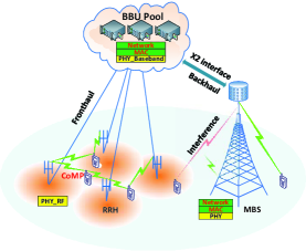
Figure 1: C-RAN architecture

As depicted in Fig. 1, the remote radio heads (RRHs) are only configured with the front radio frequency (RF) and simple symbol processing functionalities, while the other baseband physical processing and procedures of the upper layers are executed jointly in the baseband unit (BBU) pool for UEs associating with RRHs. The LPNs are simplified as RRHs through connecting to a “signal processing cloud” with high-speed fronthaul links. To coordinate the cross-tier interference between RRHs and MBSs effectively, the BBU pool is interfaced to MBSs. Such a distributed deployment and centralized processing architecture facilitates the implementation of CoMP[3] amongst RRHs of C-RANs as well as provides ubiquitous networks coverage with MBSs. Since all the RRHs in C-RANs are connected to the BBU pool, the CoMP can be realized through virtual beamforming and the beamformers can be calculated in BBU pool. Specifically, the CoMP in downlink C-RANs can be characterized into two classes[4]: joint processing (JP) and coordinated beamforming (CB). For JP, the traffic payload is shared and transmitted jointly by all RRHs within the CoMP cluster[5], which means multiple delivery of the same traffic payload from the centralized BBU pool to each cooperative RRH through capacity-limited fronthaul links. As for the CB, the traffic payload is only transmitted by the serving RRH, but the corresponding beamformer is jointly calculated at the centralized BBU pool to coordinate the interference to all other UEs within the CoMP cluster[6]. Obviously, JP achieves higher average spectrum efficiency than CB does at the expense of more fronthaul consumption, while CB requires more antennas equipped with each RRH to achieve the full intra-cluster interference coordination. However, the practical non-ideal fronthaul with limited capacity restricts the overall performances of CoMP in C-RANs.

I-A Related Works

There exists lots of literatures aiming to alleviate the fronthaul requirement of JP without the loss of interference exploitation. The authors of[7] proposed a dynamic clustered multi-cell cooperation scheme to substantially reduce the backhaul consumption by imposing restriction on the cluster size. A heuristic algorithm was proposed in[8] to dynamically select the directional cooperation links under a finite-capacity backhaul subject to the evaluation of benefits and costs, which cannot completely eliminate the undesired interference as in the full cooperation case. Both reweighed $l$-1 norm minimization method and heuristic iterative link removal algorithm were proposed in[9] to reduce the user data transfer via the capacity-limited backhaul effectively by dealing with the formulated cooperative clustering and beamforming problems, which, however, are suboptimal and still suffer from a significant performance loss. A backhaul cost metric considering the number of active directional cooperation links was adopted in[10], where the design problem is minimizing this backhaul cost metric and jointly optimizing the beamforming vectors among the cooperative BSs subject to signal-to-interference-and-noise-ratio (SINR) constraints at UEs. To make a flexible tradeoff between the cooperation gain and the backhaul consumption, a rate splitting approach under the limited backhaul rate constraints was proposed in[11], where some fraction of the backhaul capacity originally consumed by JP could be privately used to get more performance gains. Borrowing the idea in[11], the authors of[12] proposed a soft switching strategy between the JP-CoMP and CB-CoMP modes under capacity-limited backhaul. Considering the high complexity and the large signaling overhead, a distributed hard switching strategy was also proposed in[12]. To achieve a tradeoff between diversity and multiplexing gains of multiple antennas and high spectral efficiency, the authors of[13] studied both the dynamic partial JP-COMP and its corresponding resource allocation in a clustered CoMP cellular networks. Generally, for the C-RANs, the potential high spectral efficiency gain of CoMP largely depends on the quality of obtained channel state information at transmitters (CSIT) as well as the fronthaul consumption. In[14], channel prediction usefulness was analyzed and compared with channel estimation in downlink CoMP systems with backhaul latency in time-varying channels, considering both the centralized and decentralized JP-CoMP as well as the CB-CoMP.

However, the aforementioned works only focus on physical layer performance of spectral efficiency or energy efficiency and ignore the bursty traffic arrival as well as the delay requirement of delay-sensitive traffic. Therefore, the resulting control policy is adaptive to the channel state information (CSI) only and cannot guarantee good delay performance for delay-sensitive applications. In general, since the CSI could provide information regarding the channel opportunity while the queue state information (QSI) could indicate the urgency of the traffic flows, the queue-aware resource allocation should be adaptive to both the CSI and QSI. Furthermore, as the CSIT cannot be perfect in real systems, and systematic packet errors occur when the allocated data rate exceeds the instantaneous mutual information. Therefore, the issue of robustness against the uncertainty incurred by imperfect CSIT should also be considered in the resource allocation optimization.

There already have some research efforts on the queue-aware dynamic resource allocation in stochastic wireless networks. In paper[15], the authors proposed a mixed timescale delay-optimal dynamic clustering and power allocation design with downlink JP in traditional multi-cell networks. The queue-aware discontinuous transmission (DTX) and user scheduling design with downlink CB in energy-harvesting multi-cell networks was proposed in[16]. A queue-weighted dynamic optimization algorithm using Lyapunov optimization approach was proposed in[17] for the joint allocation of subframes, resource blocks, and power in the relay-based HetNets. However, all these works focus on queue-aware resource allocations in homogeneous networks or HetNets without the consideration of the imperfect CSIT. Therefore, the solutions cannot work in the C-RANs with the practical challenges of imperfect CSIT and non-ideal capacity-limited fronthaul links.

I-B Main Contributions

To the best of our knowledge, there are lack of effective signal processing techniques and dynamic radio resource management solutions for delay-sensitive traffic in C-RANs to optimize the SE, EE and delay performances, which still remains challenging and requires more investigations. Based on the aforementioned advantages and challenges of C-RANs, the efficient CoMP scheme with tradeoff between cooperation gain and fronthaul consumption will be elaborated in this paper. Furthermore, under the average power and fronthaul consumption constraints, the dynamic radio resource management with feature of queue-awareness to maintain good delay performance for delay-sensitive traffic in stochastic C-RANs will also get studied in this paper. The major contributions of this paper are as follows.

• To allow a flexible tradeoff between cooperation gain and average fronthaul consumption, the H-CoMP scheme is proposed for the delay-sensitive traffic in C-RANs by splitting the traffic payload into shared streams and private streams. By reconstructing the shared streams and private streams and optimizing the precoders and decorrelators, the shared streams and private streams can be simultaneously transmitted to obtain the maximum achievable degree of freedom (DoF) under limited fronthaul consumption.

• Motivated by[18], to minimize the transmission delay of the delay-sensitive traffic under the average power and fronthaul consumption constraints in C-RANs, the queue-aware rate and power allocation problem is formulated as an infinite horizon average cost constrained partially observed Markov process decision (POMDP). The queue-aware resource allocation policy is adaptive to both QSI and CSIT in the downlink C-RANs and can be obtained by solving a per-stage optimization for the observed system state at each scheduling frame.

• Since the optimal solution requires centralized implementation and perfect knowledge of CSIT statistics and has exponential complexity w.r.t. the number of UEs, the linear approximation of post-decision value functions involving POMDP is presented, based on which a stochastic gradient algorithm is proposed to allocate power and transmission rate dynamically with low computing complexity and high robustness against the variations and uncertainties caused by unpredictable random traffic arrivals and imperfect CSIT. Furthermore, the online learning algorithm is proposed to estimate the post-decision value functions effectively.

• The delay performances of the proposed H-CoMP and queue-aware resource allocation solution are numerically evaluated. Simulation results show that a significant delay performance gain can be achieved in the fronthaul constrained C-RANs with H-CoMP, and the queue-aware resource allocation solution is validated and effective due to the adaptiveness to both QSI and imperfect CSIT. Further, the stochastic gradient algorithms can improve the delay performances drastically, and the online learning algorithm is asymptotically converged.

The rest of this paper is organized as follows. Section II describes the system model and section III gives the design of H-CoMP scheme for the downlink C-RANs. The queue-aware resource allocation problem is formulated as POMDP in section IV and a low complexity approach is proposed in section V. The performance evaluation is conducted in section VI and section VII summarizes this paper.

Notation 1

$(.)^{T}$ and $(.)^{H}$ stand for the transpose and conjugate transpose, respectively. $(.)^{\dagger}$ stands for the pseudo-inverse. Besides, $diag(\textbf{p})$ denotes a diagonal matrix formed by the vector p.

II System Models

To optimize performances of downlink C-RANs, the transmission model, traffic queue dynamic model in the medium access control (MAC) layer, and the imperfect CSIT assumption in the physical layer are considered in this section.

II-A Transmission Model

The transmission of $M$ delay-sensitive traffic payloads in downlink C-RANs with $M$ RRHs is considered. Denote $\mathcal{M}=\{1,2,...,M\}$ as the UE set and $\mathcal{N}=\{1,2,...,M\}$ as the RRH set within the CoMP cluster. An example of C-RAN with $M=2$ is illustrated in Fig. 2. The inter-tier interferences amongst the RRHs and MBSs are controlled by setting the maximum allowable power consumption of each RRH indicated by the MBSs through the X2 interfaces, while the intra-tier interferences in C-RANs can be eliminated by implementing the CoMP. Each RRH and UE are equipped with $N_{t}$ and $N_{r}$ antennas respectively, where $M{N_{r}}\geq N_{t}>(M-1){N_{r}}$. Within the coverage of each RRH, a served UE exists and it can also be cooperatively served by the other RRHs according to the following proposed H-CoMP scheme. In this paper, the scheduling is carried out in every frame indexed by $t$ and the frame duration is $\tau$ second.

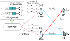
Figure 2: Workflow of resource allocation for $M$ = 2.

II-B Traffic Queue Dynamic Model

Let ${\bf{Q}}(t)=\{{Q_{1}}(t),\ldots,{Q_{M}}(t)\}$ denote the global QSI (number of bits) for $M$ queues maintained at BBU pool at the beginning of scheduling frame $t$. There will be random packet arrival ${A_{i}}(t)$ after ${G_{i}}(t)$ bits are successfully received by UE $i$ at the end of frame $t$. The random arrival process $A_{i}(t)$ is supposed to be independent identically distributed (i.i.d) over scheduling frame according to a general distribution with mean $\mathbb{E}\{{A_{i}}(t)\}={\lambda_{i}}$ and independent w.r.t $i$. Furthermore, the statistics of ${A_{i}}(t)$ is supposed to be unknown to the BBU. The queue dynamic of UE $i$ is then given by

$${Q_{i}}(t+1)=min\{{[{Q_{i}}(t)-{G_{i}}(t)]^{+}}+{A_{i}}(t),{N_{Q}}\},$$ (1)

where $[x]^{+}=max\{x,0\}$ and $N_{Q}$ is the maximum buffer size.

II-C Imperfect CSIT Assumption

Let ${{\bf{H}}_{ji}}(t)\in{\mathbb{C}^{{N_{r}}\times{N_{t}}}}$ denote the complex channel fading coefficient between RRH $i$ and UE $j$ at frame $t$ and let $\textbf{H}(t)=\{{{\bf{H}}_{ji}}(t):j\in\mathcal{M},i\in\mathcal{N}\}$ denote the global CSI. Especially, every element of ${{\bf{H}}_{ji}}(t)$ is supposed to remain constant within a scheduling frame but be i.i.d over scheduling frame. The perfect knowledge of CSI is assumed to be only obtained by the UE while the imperfect CSIT ${\bf{\hat{H}}}=\{{{\bf{\hat{H}}}_{ji}}(t)\in{\mathbb{C}^{{N_{r}}\times{N_{t}}}}:j\in\mathcal{M},i\in\mathcal{N}\}$ is obtained by the BBU pool. The rank of both ${\bf{\hat{H}}}_{ji}$ and ${\bf{H}}_{ji}$ is assumed to be $min\{N_{r},N_{t}\}$. Furthermore, the imperfect CSIT error kernel model is given by[19]

$$\Pr[{{\bf{\hat{H}}}_{ji}}|{{\bf{H}}_{ji}}]=\frac{1}{{\pi{\sigma_{ji}}}}\exp(-\frac{{|{{{\bf{\hat{H}}}}_{ji}}-{{\bf{H}}_{ji}}{|^{2}}}}{{{\sigma_{ji}}}}),$$ (2)

which is caused by duplexing delay in time division duplex (TDD) systems or quantization errors and feedback latency in frequency division duplex (FDD) systems. The above ${\sigma_{ji}}\in[0,1]$ indicates the CSIT quality. When ${\sigma_{ji}}=0$, we have ${{\bf{\hat{H}}}_{ji}}={{\bf{H}}_{ji}}$, which corresponds to the perfect CSIT case. When ${\sigma_{ji}}=1$, we have ${{\bf{\hat{H}}}_{ji}}{{\bf{H}}_{ji}^{{\dagger}}}$ = 0, which corresponds to the no CSIT case.

III Hybrid CoMP scheme

With the limited fronthaul capacity, the maximum achievable DoF can be obtained by separating the traffic payload for UE $i$ into ${L_{(i,s)}}$ shared streams ${{\bf{s}}_{(i,s)}}$ and ${L_{(i,p)}}$ private streams ${{\bf{s}}_{(i,p)}}$ and simultaneously transmitting them with optimal precoders and decorrelators, that is the hybrid CoMP (H-CoMP) scheme. More specifically, the H-CoMP allows shared streams to be shared across the RRHs with the CoMP cluster by multiple delivery through capacity-limited fronthaul links. Meanwhile, the H-CoMP makes private streams remain private to certain RRH and the precoders are jointly calculated at the BBU pool to eliminate the intra-cluster interference. Therefore, the cooperative transmission of shared streams requires significantly more fronthaul consumption than the coordinated transmission of private streams does. In the following subsections, the traffic streams splitting model, precoder calculation and decorrelator calculation with the perfect CSIT will be thoroughly elaborated.

III-A Traffic Streams Splitting Model

To make a flexible tradeoff between the cooperation gain and average fronthaul consumption, the number of shared streams and private streams should be determined with the traffic streams splitting model. With the perfect CSIT, the zero-forcing (ZF) precoder and decorrelator designs are adopted for both shared streams and private streams. In this situation, at most ${L_{M,{N_{t}},{N_{r}}}}={{N_{t}}-(M-1){N_{r}}}$ private streams can be zero-forced at RRH $i$ to eliminate interference to UE ${\rm{j}}\neq i$, i.e.

$$L_{(i,p)}\leq{L_{M,{N_{t}},{N_{r}}}}.$$ (3)

Furthermore, to fully recover the ${L_{(i,p)}}$ private streams and ${L_{(i,s)}}$ shared streams at UE $i$, the constraint

$$L_{(i,p)}+L_{(i,s)}\leq N_{r}$$ (4)

should be satisfied. With the traffic streams splitting, the proposed H-CoMP allows a flexible tradeoff between the cooperation gain and the fronthaul consumption. The achievable DoFs of different schemes are compared in table I.

TABLE I: Comparison of Achievable DoFs of Different Schemes

Scheme	Achievable DoF
CB-CoMP	$(M-1){L_{M,{N_{t}},{N_{r}}}}+{N_{r}}$
JP-CoMP	$M{N_{r}}$
H-CoMP	$\{(M-1){L_{M,{N_{t}},{N_{r}}}}+{N_{r}},...,M{N_{r}}\}$

Specifically, when $L_{(i,p)}+L_{(i,s)}=N_{r}$, the maximum DoF of $MN_{r}M$ can be achieved by the H-CoMP scheme, and when ${L_{(i,p)}}={L_{M,{N_{t}},{N_{r}}}}$, the fronthaul consumption is minimized.

Although the shared streams and private streams are superimposed in the downlink transmission of C-RANs, it is possible to eliminate the interference at RRHs and recover both of them at UEs by constructing the private streams and shared streams and designing optimal precoders and decorrelators.

Let ${{\bf{s}}_{(i,s)}}\in{\mathbb{C}^{L_{(i,s)}\times 1}}$ and ${{\bf{s}}_{(i,p)}}\in{\mathbb{C}^{L_{(i,p)}\times 1}}$ denote the shared streams and private streams respectively, where $L_{(i,s)}$ and $L_{(i,p)}$ are the number of shared streams and private streams. To facilitate the implementation of H-CoMP, the shared streams and private streams are reconstructed by inserting zero vectors as follows respectively

$${{\bf{\tilde{s}}}_{(i,s)}}={\{{\bf{s}}_{(i,s)}^{T},{{\textbf{0}}_{1\times{L_{(i,p)}}}}\}^{T}},$$ (5)

$${{\bf{\tilde{s}}}_{(i,p)}}={\{{\textbf{0}_{1\times{L_{(i,s)}}}},{\bf{s}}_{(i,p)}^{T}\}^{T}}.$$ (6)

Let ${{\bf{\tilde{W}}}_{(i,s)}}\in{\mathbb{C}^{M{N_{t}}\times{(L_{(i,s)}+L_{(i,p)})}}}$ and ${\tilde{\bf{W}}_{(i,p)}}\in{\mathbb{C}^{{N_{t}}\times{(L_{(i,p)}+L_{(i,s)})}}}$ denote the precoders for the reconstructed shared streams and reconstructed private streams of UE $i$ respectively. Define ${{\bf{\Lambda}}_{(i,s)}}=diag(\sqrt{P_{(i,s)}^{1}},\ldots,\sqrt{P_{(i,s)}^{{L_{(i,s)}}}},{\textbf{0}_{1\times{L_{(i,p)}}}})$ and ${{\bf{\Lambda}}_{(i,p)}}=diag({\textbf{0}_{1\times{L_{(i,s)}}}},\sqrt{P_{(i,p)}^{1}},\ldots,\sqrt{P_{(i,p)}^{{L_{(i,p)}}}})$, where $P_{(i,s)}$ and $P_{(i,p)}$ denote the transmission power of each shared stream and private stream for UE $i$ respectively. Then the received signal vector ${{\bf{r}}_{i}}\in{\mathbb{C}^{{N_{r}}\times 1}}$ at UE $i$ is given by

$${{\bf{r}}_{i}}=\underbrace{{{\bf{H}}_{i}}{{\tilde{\bf{W}}}_{(i,s)}}{{\bf{\Lambda}}_{(i,s)}}{{\tilde{\bf{s}}}_{(i,s)}}+{{\bf{H}}_{ii}}{{\tilde{\bf{W}}}_{(i,p)}}{{\bf{\Lambda}}_{(i,p)}}{{\tilde{\bf{s}}}_{(i,p)}}}_{{\rm{the~{}desired~{}signals~{}for~{}UE~{}i}}}$$ (7)

$$+\underbrace{\sum\limits_{j\neq i}{{{\bf{H}}_{i}}{{\tilde{\bf{W}}}_{(j,s)}}{{\bf{\Lambda}}_{(j,s)}}{{\tilde{\bf{s}}}_{(j,s)}}}}_{{\rm{the~{}interference~{}from~{}shared~{}streams}}}$$

$$+\underbrace{\sum\limits_{j\neq i}{{{\bf{H}}_{ij}}{{\tilde{\bf{W}}}_{(j,p)}}{{\bf{\Lambda}}_{(j,p)}}{{\tilde{\bf{s}}}_{(j,p)}}}}_{{\rm{the~{}interference~{}from~{}private~{}streams}}}+{{\bf{n}}_{i}},$$

where ${\textbf{H}_{i}}=[\begin{array}[]{*{20}{c}}{{\textbf{H}_{i1}}}&\cdots&{{\textbf{H}_{iM}}}\end{array}]\in{\mathbb{C}^{{N_{r}}\times M{N_{t}}}}$ is the aggregate complex channel fading coefficient vector from the $M$ cooperative RRHs to UE $i$, and ${{\bf{n}}_{i}}$ is the zero-mean unit variance complex Gaussian channel noise at UE $i$.

III-B Precoder and Decorrelator Calculation for Shared Streams

The optimal cooperative precoder at the $M$ RRHs and the decorrelator at UE $i$ should be designed to maximize the mutual information of shared streams and to eliminate the interference imposed on all the other UEs (UE $j\neq i$) as follows

$$\{{\bf{\tilde{W}}}_{{}_{(i,s)}}^{*},{\bf{\tilde{U}}}_{{}_{(i,s)}}^{*}\}=\arg\mathop{\max}\limits_{{{{\bf{\tilde{W}}}}_{(i,s)}},{{{\bf{\tilde{U}}}}_{(i,s)}}}{\log_{2}}\det[\textbf{I}+$$

$$~{}~{}~{}~{}~{}~{}~{}~{}~{}~{}~{}~{}~{}~{}~{}~{}~{}~{}~{}~{}~{}~{}~{}{{{\bf{\tilde{U}}}}_{(i,s)}}{{\bf{{\bf{H}}}}_{i}}{{{\bf{\tilde{W}}}}_{(i,s)}}{\bf{\tilde{W}}}_{{}_{(i,s)}}^{H}{\bf{H}}_{{}_{i}}^{H}{\bf{\tilde{U}}}_{{}_{(i,s)}}^{H}]$$

$$s.t.~{}~{}~{}~{}~{}~{}{{\bf{H}}_{j}}{{\bf{\tilde{W}}}_{(i,s)}}=\textbf{0}.$$ (8)

Therefore, the precoder have the form of

$${{\bf{\tilde{W}}}_{(i,s)}^{*}}={{\bf{F}}_{(i,s)}}{{{\bf{\tilde{V}}}}_{(i,s)}},$$ (9)

where ${{\bf{F}}_{(i,s)}}\in{\mathbb{C}^{M{N_{t}}\times(M{N_{t}}-(M-1){N_{r}})}}$ is given by the orthonormal basis of ${\rm{nullspace([}}{\bf{H}}_{1}^{T},\cdots,{\bf{H}}_{i-1}^{T},{\bf{H}}_{i+1}^{T}{\rm{,}}\cdots{\rm{,}}$ ${\bf{H}}_{M}^{T}{{\rm{]}}^{T}})$. Let ${{\bf{H}}_{i}}{{\bf{F}}_{(i,s)}}={{\bf{U}}_{(i,s)}}{{\bf{\Sigma}}_{(i,s)}}{\bf{V}}_{(i,s)}^{H}$ be the singular value decomposition (SVD) of equivalent channel matrix ${{\bf{H}}_{i}}{{\bf{F}}_{(i,s)}}$, where the singular values in ${{\bf{\Sigma}}_{(i,s)}}$ are sorted in a decreasing order along the diagonal, ${{\bf{\tilde{V}}}_{(i,s)}}\in{\mathbb{C}^{(M{N_{t}}-(M-1){N_{r}})\times{(L_{(i,s)}+L_{(i,p)})}}}$ is then given by the first ${L_{(i,s)}}$ columns of ${{\bf{V}}_{(i,s)}}$ as ${{\bf{\tilde{V}}}_{(i,s)}}=\{{\bf{v}}_{(i,s)}^{1},\cdots,{\bf{v}}_{(i,s)}^{{L_{(i,s)}}},{\textbf{0}}_{(M{N_{t}}-(M-1){N_{r}})\times L_{(i,p)}}\}$. Furthermore, the decorrelator ${\bf{\tilde{U}}}_{{}_{(i,s)}}^{*}$ is given by the first ${L_{(i,s)}}$ columns of ${{\bf{U}}_{(i,s)}}$ as follows

$${\bf{\tilde{U}}}_{{}_{(i,s)}}^{*}=\{{\bf{u}}_{(i,s)}^{1},\cdots,{\bf{u}}_{(i,s)}^{{L_{(i,s)}}},{\textbf{0}}_{{N_{r}}\times L_{(i,p)}}\}^{H}.$$ (10)

Then the recovered $L_{(i,s)}$ shared streams are given by the first $L_{(i,s)}$ rows of ${\bf{\tilde{U}}}_{{}_{(i,s)}}^{*}{{\bf{r}}_{i}}$.

III-C Precoder and Decorrelator Calculation for Private Streams

The optimal coordinated precoder at RRH $i$ for the private streams of UE $i$ and the decorrelator at UE $i$ should be designed to maximize the mutual information of private streams and to eliminate the interference imposed on all the other UEs (UE $j\neq i$) as follows

$$\{{\bf{\tilde{W}}}_{{}_{(i,p)}}^{*},{\bf{\tilde{U}}}_{{}_{(i,p)}}^{*}\}=\arg\mathop{\max}\limits_{{{{\bf{\tilde{W}}}}_{(i,p)}},{{{\bf{\tilde{U}}}}_{(i,p)}}}{\log_{2}}\det[\textbf{I}+$$

$$~{}~{}~{}~{}~{}~{}~{}~{}~{}~{}~{}~{}~{}~{}~{}~{}~{}{{{\bf{\tilde{U}}}}_{(i,p)}}{{\bf{{\bf{H}}}}_{ii}}{{{\bf{\tilde{W}}}}_{(i,p)}}{\bf{\tilde{W}}}_{{}_{(i,p)}}^{H}{\bf{H}}_{ii}^{H}{\bf{\tilde{U}}}_{{}_{(i,p)}}^{H}]$$

$$s.t.~{}~{}~{}~{}~{}~{}~{}{{\bf{H}}_{ji}}{{\bf{\tilde{W}}}_{(i,p)}}=\textbf{0}.$$ (11)

Therefore the precoder has the similar form of

$${{\bf{\tilde{W}}}_{(i,p)}^{*}}={{\bf{\tilde{F}}}_{(i,p)}}{{{\bf{\tilde{V}}}}_{(i,p)}},$$ (12)

where ${\bf{\tilde{F}}}_{(i,p)}=[{\textbf{0}}_{N_{t}\times(N_{r}-L_{M,N_{t},N_{r}})},{\bf{F}}_{(i,p)}]$ and ${\bf{F}}_{(i,p)}\in{\mathbb{C}^{{N_{t}}\times L_{M,N_{t},N_{r}}}}$ is given by the orthonormal basis of ${\rm{nullspace([}}{\bf{H}}_{1i}^{T},\cdots,{\bf{H}}_{i-1i}^{T},{\bf{H}}_{i+1i}^{T}{\rm{,}}\cdots{\rm{,}}{\bf{H}}_{Mi}^{T}{{\rm{]}}^{T}})$. Let ${{\bf{H}}_{ii}}{{\bf{\tilde{F}}}_{(i,p)}}={{\bf{U}}_{(i,p)}}{{\bf{\Sigma}}_{(i,p)}}{\bf{V}}_{(i,p)}^{H}$ be the SVD of equivalent channel matrix ${{\bf{H}}_{ii}}{{\bf{\tilde{F}}}_{(i,p)}}$, where the singular values in ${{\bf{\Sigma}}_{(i,p)}}$ are sorted in an increasing order along the diagonal, ${{\bf{\tilde{V}}}_{(i,p)}}\in{\mathbb{C}^{{N_{r}}\times{(L_{(i,s)}+L_{(i,p)})}}}$ is then given by the last ${L_{(i,p)}}$ columns of ${{\bf{V}}_{(i,p)}}$ as ${{\bf{\tilde{V}}}_{(i,p)}}=\{{\textbf{0}}_{{N_{r}}\times L_{(i,s)}},{\bf{v}}_{(i,p)}^{N_{r}-L_{(i,p)}+1},\cdots,{\bf{v}}_{(i,p)}^{{N_{r}}}\}$. Furthermore, the decorrelator ${\bf{\tilde{U}}}_{{}_{(i,p)}}^{*}$ is given by the last ${L_{(i,p)}}$ columns of ${{\bf{U}}_{(i,p)}}$ as follows

$${\bf{\tilde{U}}}_{{}_{(i,p)}}^{*}=\{{\textbf{0}}_{{N_{r}}\times L_{(i,s)}},{\bf{u}}_{(i,p)}^{N_{r}-L_{(i,p)}+1},\cdots,{\bf{u}}_{(i,p)}^{N_{r}}\}^{H}.$$ (13)

Then the recovered $L_{(i,p)}$ private streams are given by the last $L_{(i,p)}$ rows of ${\bf{\tilde{U}}}_{{}_{(i,p)}}^{*}{{\bf{r}}_{i}}$.

Remark 1

(The Interference Nulling Between Shared Streams and Private Streams) Although the interference nulling constraints are not explicitly imposed, the interference between shared streams and private streams of UE $i$ can be still eliminated due to the fact that ${\bf{\tilde{U}}}_{{}_{(i,s)}}^{*}{{\tilde{\bf{W}}}_{(i,p)}}{{\bf{\Lambda}}_{(i,p)}}{{\tilde{\bf{s}}}_{(i,p)}}=\textbf{0}$ and ${\bf{\tilde{U}}}_{{}_{(i,p)}}^{*}{{\tilde{\bf{W}}}_{(i,s)}}{{\bf{\Lambda}}_{(i,s)}}{{\tilde{\bf{s}}}_{(i,s)}}=\textbf{0}$.

III-D The Power Consumption and Transmission Rate

To support the cooperative transmission of $a$-th shared stream from $M$ RRHs to UE $j$, the power contributed by RRH $i$ is given by $P_{(j,s)}^{a}\rho_{(j,i)}^{a}$, where $P_{(j,s)}^{a}$ denote the total power to transmit the $a$-th shared stream to UE $i$ and $\rho_{(j,i)}^{a}=\sum\nolimits_{x=1}^{{N_{t}}}{|{{[{{\bf{\tilde{W}}}^{*}_{(j,s)}}]}_{((i-1){N_{t}}+x,a)}}{|^{2}}}$ denote the contribution by RRH $i$. To support the coordinated transmission of $a$-th private stream from RRH $i$ to UE $i$, the power of $P_{(i,s)}^{a}$ is needed. Therefore, with the proposed H-CoMP scheme, the total transmit power consumption at RRH $i$ is given by

$$P_{i}=\sum\nolimits_{a=1}^{{L_{(i,p)}}}{P_{(i,p)}^{a}}+\sum\nolimits_{j=1}^{M}{\sum\nolimits_{a=1}^{{L_{(j,s)}}}{P_{(j,s)}^{a}\rho_{(j,i)}^{a}}}.$$ (14)

In practice, both the precoders and decorrelators are calculated at the BBU pool with the imperfect CSIT, which will cause uncertain residual interference to the recovered streams. By treating the uncertain interference as noise, the mutual information of $a$-th shared stream at ${\bf{s}}_{(i,s)}^{a}$ UE $i$ is given by

$$C_{(i,s)}^{a}={\log_{2}}(1+{{\varphi}_{(i,s)}^{a}}P_{(i,s)}^{a}/(1+I_{(i,s)}^{a})),$$ (15)

where $\varphi_{(i,s)}^{a}=|{\bf{\tilde{U}}}_{(i,s)}^{a}{{\bf{H}}_{i}}{\bf{\tilde{W}}}_{(i,s)}^{a}{|^{2}}$, ${\bf{\tilde{U}}}_{(i,s)}^{a}$ and ${\bf{\tilde{W}}}_{(i,s)}^{a}$ is the $a$-th row of ${\bf{\tilde{U}}}_{(i,s)}^{*}$ and $a$-th column of ${\bf{\tilde{W}}}_{(i,s)}^{*}$ respectively, $I_{(i,s)}^{a}$ is the residual interference incurred by the imperfect CSIT. The mutual information of $a$-th private stream ${\bf{s}}_{(i,p)}^{a}$ of UE $i$ is given in a similar way. Due to the uncertainties of mutual information, the data rate successfully transmitted to UE $i$ is given by

$${G_{i}}=({R_{(i,s)}}\textbf{1}({R_{(i,s)}}\leq{C_{(i,s)}})+{R_{(i,p)}}\textbf{1}({R_{(i,p)}}\leq{C_{(i,p)}}))\tau,$$ (16)

where ${C_{(i,s)}}=\sum\nolimits_{a=1}^{{L_{(i,s)}}}{C_{(i,s)}^{a}}$ and ${C_{(i,p)}}=\sum\nolimits_{a=1}^{{L_{(i,p)}}}{C_{(i,p)}^{a}}$ are the mutual information for shared streams and private streams respectively. ${R_{(i,s)}}$ and ${R_{(i,p)}}$ are the allocated data rate for shared streams and private streams of UE $i$ respectively.

IV Formulation of Queue-aware Control Problem

To meet the urgency of the delay-sensitive traffic payloads and reduce the occurrence of packet transmission failure in the downlink C-RANs, the queue-aware resource allocation problem based on the observed system states (QSI and CSIT) will be formulated in this section.

IV-A Feasible Stationary Control Policy

Considering the inter-tier interference imposed by RRHs and the energy efficient transmission of delay-sensitive traffic, the feasible resource allocation policy should satisfy the following average power consumption constraints

$${P_{i}}{\rm{(}}\Omega{\rm{)=}}\mathop{lim}\limits_{T\to\infty}{sup}\frac{1}{T}\sum\limits_{t=1}^{T}{{{\mathbb{E}}^{\Omega}}[{P_{i}}(t)]}\leq P_{i}^{\max},$$ (17)

where ${\mathbb{E}^{\Omega}}$ indicates that the expectation is taken w.r.t the measure induced by policy $\Omega$, ${P_{i}}(t)$ is the total power consumption of RRH $i$ to support the H-CoMP transmission, and $P_{i}^{\max}$ is the maximum average power consumption indicated by MBSs. Furthermore, by varying the maximum average power consumption of each RRH, cross-tier interference could be well controlled to maintain desirable average QoS requirement for macro UEs.

It is worth noting that compared with the fronthaul consumption for traffic payload sharing, that for signaling delivery is negligible. Due to the capacity-limited fronthaul links of C-RANs, the feasible resource allocation policy also should satisfy the following average fronthaul consumption constraints

$$R_{i}^{f}(\Omega)\!=\!\mathop{lim}\limits_{T\to\infty}\!{sup}\frac{1}{T}\sum\limits_{t=1}^{T}\!{{{\mathbb{E}}^{\Omega}}[{R_{(i,p)}}(t)\!+\!\sum\limits_{j}\!{{R_{(j,s)}}(t)}]}\!\leq\!R_{i}^{\max},$$ (18)

where ${R_{(i,p)}}(t)+\sum\nolimits_{j\in\mathcal{M}}{{R_{(j,s)}}(t)}$ is the total data rate to be delivered to RRH $i$ through the fronthaul link connecting RRH $i$ to BBU pool, and $R_{i}^{\max}$ is the maximum average fronthaul consumption.

With the aforementioned resource constraints, the feasible stationary resource allocation policy for C-RANs is defined as follows.

Definition 1

(Stationary Resource Allocation Policy) A feasible stationary resource allocation policy $\Omega({\bf{\hat{S}}})=\{{\Omega_{R}}({\bf{\hat{S}}}),{\Omega_{P}}({\bf{\hat{S}}})\}$ is a mapping from the global observed system states ${\bf{\hat{S}}}=\{{\bf{Q}},{\bf{\hat{H}}}\}$ instead of the global system states ${\bf{S}}=\{{\bf{Q}},{\bf{H}},{\bf{\hat{H}}}\}$ to the resource allocation actions, where ${\Omega_{P}}({\bf{\hat{S}}})=\{{{{P}}^{a}_{(i,p)}},{{{P}}^{b}_{(i,s)}}:1\leq a\leq L_{(i,p)},1\leq b\leq L_{(i,s)},i\in M\}$ and ${\Omega_{R}}({\bf{\hat{S}}})=\{{{{R}}_{(i,p)}},{{{R}}_{(i,s)}}:i\in M\}$ are the power allocation policy and rate allocation policy subject to average power consumption constraints and average fronthaul consumption constraints.

Given the feasible stationary resource allocation policy $\Omega({\bf{\hat{S}}})$, the induced random process ${\bf{S}}=\{{\bf{Q}},{\bf{H}},{\bf{\hat{H}}}\}$ is a controlled Markov chain with the transition probability as follows

$$\Pr\!\{{\bf{S}}(t\!+\!1)|{\bf{S}}(t),\Omega({\bf{\hat{S}}}(t))\}\!=\Pr\{{\bf{\hat{H}}}(t\!+\!1),{\bf{H}}(t\!+\!1)\}$$

$$\Pr\{{\bf{Q}}(t\!+\!1)|{\bf{S}}(t),\Omega({\bf{\hat{S}}}(t))\}.$$ (19)

Apparently, the queue dynamics of the $M$ UEs served by C-RAN are coupled with each other via $\Omega({\bf{\hat{S}}}(t))$.

IV-B Problem Formulation

With the positive weighting factors $\{{\beta}_{i}\}$ ,which indicates the relative importance of delay requirement among the $M$ users, the queue-aware resource allocation problem with average power consumption constraints and average fronthaul consumption constraints can be formulated as the following problem.

Problem 1

(Queue-aware Resource Allocation Problem)

$${\min_{\Omega}}D({\bf{\beta}},\Omega)=\mathop{lim}\limits_{T\to\infty}{sup}\frac{1}{T}\sum\limits_{t=1}^{T}{{{\mathbb{E}}^{\Omega}}[\sum\limits_{i\in M}{{\beta_{i}}\frac{{{Q_{i}}}}{{{\lambda_{i}}}}}]}$$ (20)

$$s.t.\rm{~{}~{}the~{}constraints~{}(17)~{}and~{}(18)~{}for~{}each~{}RRH},$$

where the $\frac{{{Q_{i}}}}{{{\lambda_{i}}}}$ in objective function is the average traffic delay cost for UE $i$ by Little’s Law.

With the average power consumption constraints and average fronthaul consumption constraints in Problem 1, the occurrence of extreme instantaneous power and fronthaul consumption tends to be impossible. Furthermore, the feasible stationary resource allocation policy is defined on the observed system states ${\bf{\hat{S}}}=\{{\bf{Q}},{\bf{\hat{H}}}\}$. Therefore, problem 1 is a constrained partially observed MDP (POMDP)[20], which will be solved by the following general approach.

IV-C General Approach with MDP

Using the Lagrange duality theory, the Lagrange dual function of problem 1 is defined as

$$J(\gamma)\!=\!\mathop{\min}\limits_{\Omega}L(\beta,\gamma,\Omega({\bf{\hat{S}}}))\!=\!\mathop{lim}\limits_{T\to\infty}{sup}\frac{1}{T}\!\sum\limits_{t=1}^{T}{{{\mathbb{E}}^{\Omega}}[g({\bf{\beta}},{\bf{\gamma}},\Omega({\bf{\hat{S}}}))]},$$ (21)

where $g({\bf{\beta}},{\bf{\gamma}},\Omega({\bf{\hat{S}}}))=\sum\limits_{i}{({\beta_{i}}\frac{{{Q_{i}}}}{{{\lambda_{i}}}})+}{\gamma_{(i,P)}}({{\rm{P}}_{i}}-P_{i}^{\max})+{\gamma_{(i,R)}}(R_{i}^{f}-R_{i}^{\max})$ is the per-stage system cost and ${\gamma_{(i,P)}}$ and ${\gamma_{(i,R)}}$ are the non-negative Lagrange multipliers (LMs) w.r.t the power consumption constraints and fronthaul consumption constraints. Then the dual problem of problem 1 is given by

$$\mathop{\max}\nolimits_{\gamma}J(\gamma).$$ (22)

Although (21) is an unconstrained POMDP, the solution is generally nontrivial. To substantially reduce the global observed system states space, the partitioned actions are defined as follows with the i.i.d. property of the CSIT.

Definition 2

(Partitioned Actions) Given the stationary resource allocation policy $\Omega$, $\Omega({\bf{Q}})=\{\Omega({\bf{\hat{S}}}):\forall{\bf{\hat{H}}}\}$ is defined as the collections of power and rate allocation actions for all possible CSIT ${\bf{\hat{H}}}$ on a given QSI Q, therefore $\Omega$ is equal to the union of all partitioned actions. i.e. $\Omega={\cup}_{\textbf{Q}}{{\Omega}(\textbf{Q})}$.

As the distribution of the traffic arrival process is unknown to the BBU, the post-decision state potential function instead of potential function will be introduced in the following theorem to derive the queue-aware resource allocation policy of eq. (21).

Theorem 1

(Equivalent Bellman Equation)
(a)Given the LMs, the unconstrained POMDP problem can be solved by the equivalent Bellman equation as follows

$$U({\bf{\tilde{Q}}})+\theta=\sum\nolimits_{\bf{A}}{\Pr({\bf{A}})}\mathop{min}\limits_{\Omega(\textbf{Q})}g(\bf{\beta},{\bf{\gamma}},\textbf{Q},{\Omega(\textbf{Q})})$$

$$+\sum\nolimits_{{\bf{\tilde{Q}}}^{\prime}}{\Pr\{{\bf{\tilde{Q}}}^{\prime}|\textbf{Q},{\Omega(\textbf{Q})}\}U({\bf{\tilde{Q}}}^{\prime})},$$ (23)

where $g(\bf{\beta},{\bf{\gamma}},{\bf{Q}},\Omega({\bf{Q}}))=\mathbb{E}[g({\bf{\beta}},{\bf{\gamma}},\Omega({\bf{\hat{S}}}))|{\bf{Q}}]$ is the conditional per-stage cost and $\Pr\{{\bf{\tilde{Q}}}^{\prime}|{\bf{Q}},{\Omega(\textbf{Q})}\}=\mathbb{E}[\Pr[{\bf{Q}}^{\prime}|{\bf{H}},{\bf{Q}},\Omega({\bf{\hat{S}}})]|{\bf{Q}}]$ is the conditional average transition kernel, $U({\bf{\tilde{Q}}})$ is the post-decision value function. ${\bf{\tilde{Q}}}$ is the post-decision state and ${\bf{\tilde{Q}}}^{\prime}={({\bf{Q}}-{\bf{G}})^{+}}$ is the next post-decision state, where ${\bf{Q}}=\min\{{\bf{\tilde{Q}}}+{\bf{A}},{N_{Q}}\}$ and ${\bf{G}}=\{G_{i}:i\in\mathcal{M}\}$.

(b)If there exists unique $(\theta,\{U({\bf{\tilde{Q}}})\})$ that satisfies (23), then $\theta=\mathop{min}\limits_{\Omega(\textbf{Q})}{\mathbb{E}}[g(\bf{\beta},{\bf{\gamma}},{\bf{Q}},\Omega({\bf{Q}}))$ is the optimal average per-stage cost for the unconstrained POMDP and the optimal resource allocation policy $\Omega$ is obtained by minimizing R.H.S of (23).

Proof:

Please refer to Appendix A ∎

Remark 2

(The Zero Duality Gap) Although the objective function of problem 1 is not convex w.r.t the stationary resource control policy, the duality gap between the dual problem and primal problem is zero when the condition Theorem 1 (b) is established, which implies that the primal optimal resource control policy can be obtained by solving the equivalent Bellman equation of the dual optimal problem.

Remark 3

(The Computational Complexity) Solving the equivalent Bellman equation involves ${N_{Q}}^{M}+1$ unknowns $(\theta,\{U({\bf{\tilde{Q}}})\})$ and ${N_{Q}}^{M}$ nonlinear fixed point equations, which means exponential state space, enormous computational complexity and full knowledge of system states transition probability in (19). Therefore, a low complexity solution based on linear approximation and online learning of post-decision value functions will be further studied.

V Low Complexity Approach

In this section, to substantially reduce the enormous computing complexity in centralized BBU pool, the linear approximation of post-decision value functions is utilized, upon which a stochastic gradient algorithm is proposed to obtain the QAH-CoMP policy and an online learning algorithm is proposed to estimate the post-decision value functions.

V-A Linear Approximation of Post-decision Value Functions

The linear approximation of post-decision value functions is defined by the sum of the per-queue value functions as follows[21]

$$U({\bf{\tilde{Q}}})\approx\sum\nolimits_{i\in\mathcal{M}}{{U_{i}}({{\tilde{Q}}_{i}})},$$ (24)

where ${U_{i}}({\tilde{Q}_{i}})$ is the per-queue post-decision value functions which satisfies the following per-queue fixed point Bellman equation

$${U_{i}}({{{\rm{\tilde{Q}}}}_{i}})\!+\!{\theta_{i}}\! =\!\sum\nolimits_{{A_{i}}}{\Pr({A_{i}})}\mathop{min}\limits_{{\Omega}_{i}(Q_{i})}[{g_{i}}({\beta_{i}},{{\bf{\gamma}}_{i}},{Q_{i}},{{\Omega}_{i}})$$ (25)

$$+\sum\nolimits_{{{\tilde{Q}}_{i}}^{\prime}}{\Pr\{\tilde{Q}{{}^{\prime}_{i}}|{Q_{i}},{{\Omega}_{i}}\}U(\tilde{Q}{{}^{\prime}_{i}})}],$$

where ${g_{i}}({\beta_{i}},{{\bf{\gamma}}_{i}},{Q_{i}},{{\Omega}_{i}})=\mathbb{E}[{\beta_{i}}\frac{{{Q_{i}}}}{{{\lambda_{i}}}}+{\gamma_{(i,P)}}(\sum\limits_{a=1}^{{L_{(i,s)}}}{P_{(i,s)}^{a}\rho_{(i,i)}^{a}}+\sum\limits_{a=1}^{{L_{(i,p)}}}{P_{(i,p)}^{a}}-P_{i}^{\max})+\sum\limits_{j\in\mathcal{M},j\neq i}{{\gamma_{(j,P)}}}$ $\sum\limits_{a=1}^{{L_{(i,s)}}}{P_{(i,s)}^{a}\beta_{(i,j)}^{a}}+{\gamma_{(i,R)}}({R_{(i,p)}}(t)+\sum\limits_{j\in\mathcal{M}}{{R_{(j,s)}}(t)}-R_{i}^{\max})|Q_{i}]$ is the per-queue per-stage cost function. ${Q_{i}}=\min\{{\tilde{Q}_{i}}+{A_{i}},{N_{Q}}\}$ is the pre-decision state and $\tilde{Q}{{}^{\prime}_{i}}={({Q_{i}}-{G_{i}})^{\dagger}}$ is the next post-decision state. The optimality of linear approximation is established in the following lemma.

Lemma 1

(The Optimality of Linear Approximation) The linear approximation is optimal only when the CSIT is perfect, which means the interference is completely eliminated with H-CoMP scheme, therefore, the queue dynamics of $M$ UEs are decoupled.

Proof:

Please refer to Appendix B. ∎

Generally, the error variance ${\sigma}_{ji}$ of the imperfect CSIT can not be large, therefore the linear approximation is asymptotically accurate with sufficiently small error variance of CSIT.

Remark 4

(The Computing Complexity) With the linear approximation, the calculation of the post-decision value functions in BBU pool is alleviated from exponential complexity $\mathcal{O}((N_{Q}+1)^{M})$ to polynomial complexity $\mathcal{O}((N_{Q}+1)M)$.

V-B Low Complexity QAH-CoMP Policy

With the combination of the linear approximation and equivalent Bellman equation (23), the QAH-CoMP policy can be obtained by solving the following per-stage optimization for every observed system state, which is summarized as the following corollary.

Corollary 1 (Per-Stage Optimization)

With the observation of current system states, the per-stage optimization is given by

$${\Omega^{*}}({\bf{\hat{S}}})\!=\!\{\Omega_{P}^{*}({\bf{\hat{S}}}),\Omega_{R}^{*}({\bf{\hat{S}}})\}\!=\!{\rm{arg}}\!\!\!\mathop{min}\limits_{\Omega_{P}({\bf{\hat{S}}}),\Omega_{R}({\bf{\hat{S}}})}\!\!\!B({\bf{\hat{S}}},\!{\Omega_{P}({\bf{\hat{S}}}),\Omega_{R}({\bf{\hat{S}}})}),$$ (26)

where $B({\bf{\hat{S}}},{\Omega_{P}({\bf{\hat{S}}}),\Omega_{R}({\bf{\hat{S}}})})=\sum\limits_{i\in\mathcal{M}}{\{{\gamma_{(i,P)}}P_{i}{\gamma_{(i,R)}}({R_{(i,p)}}(t)}$ ${+\sum\limits_{j}{{R_{(j,s)}}(t)})+{\mathbb{E}}[{{\bf{1}}_{(i,s)}}{{\bf{1}}_{(i,p)}}]({U_{i}}({Q_{k}}-{\tau R_{(i,s)}}}{-\tau{R_{(i,p)}})}$ ${-{U_{i}}({Q_{k}}-\tau{R_{(i,p)}})-{U_{i}}({Q_{k}}-\tau{R_{(i,s)}})+{U_{i}}({Q_{k}}))}+{\mathbb{E}}[{{\bf{1}}_{(i,s)}}]({U_{i}}({Q_{k}}-\tau{R_{(i,s)}})-{U_{i}}({Q_{k}}))+{\mathbb{E}}[{{\bf{1}}_{(i,p)}}]({U_{i}}({Q_{k}}-\tau{R_{(i,p)}})-{U_{i}}({Q_{k}}))\}$ is the per-stage objective, ${{\bf{1}}_{(i,p)}}={\bf{1}}({R_{(i,p)}}\leq{C_{(i,p)}})$ and ${{\bf{1}}_{(i,p)}}={\bf{1}}({R_{(i,s)}}\leq{C_{(i,s)}})$ are the indicator functions.

The per-stage optimization above is intractable due to that the expectation $\mathbb{E}$ required the explicit knowledge of CSIT errors in BBU pool. To deal with this challenge, the per-stage optimization problem can be solved by the following stochastic gradient algorithm[22].

Algorithm 1

(Stochastic Gradient Algorithm)

At each frame $t>1$, the queue-aware power and rate allocations for each UE can be obtained as the following iteration

$$e_{i}^{t}({{\bf{\hat{S}}}_{i}})={[e_{i}^{t-1}({{\bf{\hat{S}}}_{i}})-{\gamma_{e}}(t-1)d(e_{i}^{t-1}({{\bf{\hat{S}}}_{i}}))]^{+}},$$ (27)

where ${\gamma_{e}}(t)$ is the step size satisfying ${\gamma_{e}}(t)>0,\sum\nolimits_{t}{{\gamma_{e}}(t)}=\infty,\sum\nolimits_{t}{{{({\gamma_{e}}(t))}^{2}}}<\infty$ and $d(e_{i}^{t}({{\bf{\hat{S}}}_{i}}))$ is the stochastic gradient w.r.t power and rate allocation, which is summarized as follows

$$\left\{\begin{array}[]{l}\frac{{\partial B({\bf{\hat{S}}},{\Omega_{P}({\bf{\hat{S}}}),\Omega_{R}({\bf{\hat{S}}})})}}{{\partial P_{(i,p)}^{a}}}={\gamma_{(i,P)}}+\frac{{\partial{h_{i}}({\bf{\hat{S}}},{\Omega_{P}({\bf{\hat{S}}}),\Omega_{R}({\bf{\hat{S}}})})}}{{\partial P_{(i,p)}^{a}}}\\ \frac{{\partial B({\bf{\hat{S}}},{\Omega_{P}({\bf{\hat{S}}}),\Omega_{R}({\bf{\hat{S}}})})}}{{\partial P_{(i,s)}^{a}}}={\gamma_{(i,P)}}\rho_{(i,i)}^{a}+\frac{{\partial{h_{i}}({\bf{\hat{S}}},{\Omega_{P}({\bf{\hat{S}}}),\Omega_{R}({\bf{\hat{S}}})})}}{{\partial P_{(i,s)}^{a}}}\\ ~{}~{}~{}~{}~{}~{}~{}~{}~{}~{}~{}~{}~{}~{}~{}~{}~{}~{}~{}~{}~{}~{}+\sum\limits_{j\neq i,j\in\mathcal{M}}{{\gamma_{(j,P)}}\rho_{(i,j)}^{a}}\\ \frac{{\partial B({\bf{\hat{S}}},{\Omega_{P}({\bf{\hat{S}}}),\Omega_{R}({\bf{\hat{S}}})})}}{{\partial{R_{(i,p)}}}}={\gamma_{(i,R)}}+\frac{{\partial{h_{i}}({\bf{\hat{S}}},{\Omega_{P}({\bf{\hat{S}}}),\Omega_{R}({\bf{\hat{S}}})})}}{{\partial{R_{(i,p)}}}}\\ \frac{{\partial B({\bf{\hat{S}}},{\Omega_{P}({\bf{\hat{S}}}),\Omega_{R}({\bf{\hat{S}}})})}}{{\partial{R_{(i,p)}}}}={\gamma_{(i,R)}}+\frac{{\partial{h_{i}}({\bf{\hat{S}}},{\Omega_{P}({\bf{\hat{S}}}),\Omega_{R}({\bf{\hat{S}}})})}}{{\partial{R_{(i,p)}}}}\\ ~{}~{}~{}~{}~{}~{}~{}~{}~{}~{}~{}~{}~{}~{}~{}~{}~{}~{}~{}~{}~{}~{}+\sum\limits_{j\neq i,j\in\mathcal{M}}{{\gamma_{(j,R)}}}\end{array}\right.,$$ (28)

where ${h_{i}}({\bf{\hat{S}}},{\Omega_{P}({\bf{\hat{S}}}),\Omega_{R}({\bf{\hat{S}}})})={{\bf{1}}_{(i,s)}}({U_{i}}({Q_{k}}-\tau{R_{(i,s)}})-{U_{i}}({Q_{k}}))+{{\bf{1}}_{(i,p)}}({U_{i}}({Q_{k}}-\tau{R_{(i,p)}})-{U_{i}}({Q_{k}}))+{{\bf{1}}_{(i,s)}}{{\bf{1}}_{(i,p)}}({U_{i}}({Q_{k}}-\tau{R_{(i,s)}}-\tau{R_{(i,p)}})-{U_{i}}({Q_{k}}-\tau{R_{(i,s)}})-{U_{i}}({Q_{k}}-\tau{R_{(i,p)}})+{U_{i}}({Q_{k}}))$.

When ${\bf{\hat{H}}}={\bf{H}}$, there is no interference under the H-CoMP with perfect CSIT, and $d(e_{i}^{t}({{\bf{\hat{S}}}_{i}}))$ is deterministic instead of stochastic. Using the standard gradient update argument, the gradient search converges to a local optimum as $t\to\infty$. Therefore, the Algorithm 1 gives the asymptotically local optimal solution at small CSIT errors, which means that the explicit knowledge of imperfect CSIT is unnecessary and it is robust against the uncertainties caused by imperfect CSIT.

Remark 5

(Feedback-Assisted Realization of Algorithm 1) The calculation of stochastic gradient (28) in BBU pool requires some items regarding the indicator functions ${\bf{1}}_{(i,s)}$ and ${\bf{1}}_{(i,p)}$ and the differential of post-decision value functions $U_{i}^{{}^{\prime}}({\tilde{Q}_{i}})$. At each frame $t$, the indicator functions are unknown by BBU pool and have to be fed back from UEs, which is feasible due to that there are existing built-in mechanisms in wireless networks for these ACK/NACK feedback from UEs. In addition, since there is no closed-form expression of post-decision value function $U_{i}^{{}^{\prime}}({\tilde{Q}_{i}})$, its differential can be estimated as follows

$$U_{i}^{{}^{\prime}}({\tilde{Q}_{i}})=U_{i}({\tilde{Q}_{i}})-U_{i}({\tilde{Q}_{i}}-1),$$ (29)

where the online learning of $U_{i}({\tilde{Q}_{i}})$ will be elaborated in next subsection.

V-C Online Learning of Per-queue Post-decision Value Functions

The post-decision value functions are critical to the derivation of queue-aware resource allocation policy for C-RANs, which can be obtained by solving $N_{Q}$ fixed point nonlinear Bellman equations with $N_{Q}+1$ variables. The offline calculation requires the explicit knowledge of conditional average transition kernel, which is infeasible. In this section, with the realtime observation of QSI and CSIT, the online learning of per-queue post-decision value functions is proposed based on the equation (25). Meanwhile, with the realtime resource control actions, the LMs are updated to make sure the average power consumption constraints and average fronthaul consumption constraints are satisfied[23]. The online learning of per-queue value functions and the update of LMs at centralized BBU pool are described as follows.

Algorithm 2

(Online Learning of Per-Queue Value Functions and Update of LMs)

Step 1 (Initialization)

Set $t=0$, the per-queue post-decision value functions $\{U_{i}^{0}({{\tilde{Q}}_{i}})\}$ and LMs $\{\gamma_{(i,P)}^{0},\gamma_{(i,R)}^{0}\}>0$ are initialized at the centralized BBU pool.

Step 2 (Queue-Aware Resource Allocation)

At the beginning of the $t$-th frame, given fixed $\{{\eta_{j}}(n)\}$, the queue-aware power and rate allocation for downlink H-CoMP transmission are determined at the BBU pool using the stochastic gradient algorithm in (28).

Step 3 (Online Learning of $U_{i}^{t+1}({{\tilde{Q}}_{i}})$)

With the observation of post-decision QSI $\{{{\tilde{Q}}_{i}}\}$ and pre-decision QSI $\{{Q_{i}}\}$, the per-queue post-decision value function $U_{i}({{\tilde{Q}}_{i}})$ is online learned at BBU pool (30) for each traffic queue as follows

$$U_{i}^{t+1}({{\tilde{Q}}_{i}}) =U_{i}^{t}({{\tilde{Q}}_{i}})+{\zeta_{u}}(t)[{g_{i}}(\gamma_{i}^{t},{{{\bf{\hat{S}}}}_{i}},{P_{i}},{R_{i}}+U_{i}^{t}({Q_{i}}-{U_{i}})$$ (30)

$$-U_{i}^{t}(\tilde{Q}_{i}^{0})-U_{i}^{t}({{\tilde{Q}}_{i}})].$$

Step 4 (Update of $\{\gamma_{(i,P)}^{t+1},\gamma_{(i,R)}^{t+1}\}$)

With the observation of power and rate allocation, the $\{\gamma_{(i,P)}^{t+1}\}$ and $\{\gamma_{(i,R)}^{t+1}\}$ are updated according to eq.(31) and eq.(32) at the BBU pool for the power consumption constraints and fronthaul consumption constraints respectively,

$$\gamma_{(i,P)}^{t+1}\!=\!{[\gamma_{(i,P)}^{t}+{\zeta_{\gamma}}\!(t)({P_{i}}-P_{i}^{\max})]^{+}},$$ (31)

$$\gamma_{(i,R)}^{t+1}\!=\!{[\gamma_{(i,R)}^{t}\!+\!{\zeta_{\gamma}}\!(t)({R_{(i,p)}}(t)\!+\!\sum\nolimits_{j\in\mathcal{M}}{{R_{(j,s)}}\!(t)}\!-\!R_{i}^{\max})]^{+}}.$$ (32)

Step 5 (Termination)

Set $t=t+1$ and continue to step 2 until certain termination condition is satisfied.

The ${\zeta_{u}}(t)$ and ${\zeta_{\gamma}}(t)$ in step 3 and step 4 is the iterative step size of post-decision value functions and LMs respectively. To make sure the convergence of iteration, they should satisfy the conditions as follows[24]:

$${\zeta_{u}}(t)>0,\sum\nolimits_{t}{{\zeta_{u}}(t)}=\infty,$$ (33)

$${\zeta_{\gamma}}(t)>0,\sum\nolimits_{t}{{\zeta_{\gamma}}(t)}=\infty,$$ (34)

$$\sum\nolimits_{t}{({{({\zeta_{u}}(t))}^{2}}+}{({\zeta_{\gamma}}(t))^{2}})<\infty,$$ (35)

$$\mathop{\lim}\limits_{t\to\infty}\frac{{{\zeta_{\gamma}}(t)}}{{{\zeta_{u}}(t)}}=0.$$ (36)

Remark 6 (Two Timescales of Iterations)

The condition (36) implies that the LMs are relatively static during the iteration of per-queue value functions. Therefore the iteration of post-decision value functions and the iteration of LMs are done simultaneously but over two different time scales[25].

It is a remarkable fact that the size of per-queue states(in bits) is still large. To accelerate the estimation of each post-state value function, the per-queue QSI space ${{\mathcal{Q}}_{i}}$ is partitioned into $N$ regions as (37)

$${{\mathcal{Q}}_{i}}=\bigcup\nolimits_{n=1}^{N}{{{\mathcal{R}}_{n}}}.$$ (37)

Therefore, the average value function w.r.t each region is online learned instead, then the post-decision value function of each state within the region can be estimated by interpolation method after each iteration.

VI Performances Evaluation

In this section, simulations are conducted to compare the performances of the proposed QAH-CoMP with various baselines in C-RANs. The delay-sensitive traffic packet arrival follows a Poisson distribution and the corresponding packet size follows an exponential distribution, which is a widely adopted traffic model[18]. The mean size of traffic packet is 4Mbits and the maximum buffer size is 32Mbits. The CSI ${{\bf{H}}_{ij}}$ is uniformly distributed over a state space ${\mathcal{H}}^{N_{r}\times N_{t}}$ and the error variance of the imperfect CSIT is ${\varepsilon_{e}}=0.05$. The configuration of multi-antennas is given by $\{{N_{t}}=5,{N_{r}}=2\}$ and the cluster size is $M$ = 3. Therefore, with the stream splitting of the H-CoMP scheme, there are one shared stream and one private stream to be transmitted for each UE. The total bandwidth of simulated C-RAN is 20MHz and the scheduling frame duration is 10ms. The noise power is -15dBm.

Three baselines are considered in the simulations: CB-CoMP, JP-CoMP, and channel-aware resource allocation with H-CoMP (CAH-CoMP). All these three baselines carry out rate and power allocation to maximize the average system throughput with the same fronthaul capacity and average power consumption constraint as the proposed QAH-CoMP. For the CB-CoMP baseline, the BBU pool calculates the coordinated beamformer for each RRH to eliminate the dominating intra-cluster interference. For the CAH-CoMP baseline, the proposed H-CoMP transmission is adopted, while the power allocation and rate allocation are only adaptive to CSIT.

Fig. 3 compares the delay performance of the four schemes with different packet arrival rate. The average packet delay of all the schemes increases as the average packet arrival rate increases. Compared with CB, the delay outperformance of JP weakens as the packet arrival rate increases, which is due to the fact that the fronthaul capacity becomes relatively limited with the increasing packet arrival rate. Apparently, the performance gain of QAH-CoMP compared with CAH-CoMP is contributed by power and rate allocation with the consideration of both urgent traffic flows and imperfect CSIT.

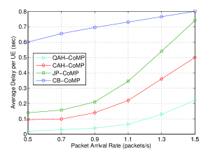
Figure 3: Average packet delay vs. packet arrival rate, the maximum fronthaul consumption is $R_{i}^{max}$ = 20Mbits/s, the maximum transmit power is $P_{i}^{max}$ = 10dBm.

Fig. 4 compares the delay performance of the four schemes with different maximum transmit power. The figure depicts the medium fronthaul consumption regime, in which JP-CoMP outperforms CS-CoMP due to the higher spectrum efficiency. CAH-CoMP outperforms both CS-CoMP and JP-CoMP while the outperformance of CAH-CoMP is not so obvious with relative enough fronthaul capacity. It can be observed that there is significant performance gain of the proposed QAH-CoMP compared with all the baselines across a wide range of the maximum power consumption.

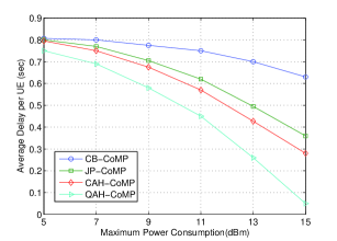
Figure 4: Average packet delay vs. maximum transmit power, the packet arrival rate is ${\lambda}_{i}$ = 2.5 packets/s, the maximum fronthaul consumption is $R_{i}^{max}$ = 30Mbits/s.

Fig. 5 compares the delay performance of the four schemes with different maximum fronthaul consumption. The figure depicts the small fronthaul consumption regime, in which CAH-CoMP clearly outperforms both CS-CoMP and JP-CoMP, which is contributed by the flexible adjustment of cooperation level when the fronthaul capacity is limited. Note that the JP-CoMP has worse delay performance than CS-CoMP due to limited fronthaul capacity at first but it eventually gets performance improvement with increasing fronthaul capacity. Similarly, due to the queue-aware power and rate allocation, QAH-CoMP substantially outperforms the three baselines.

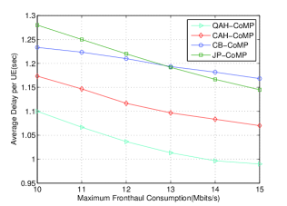
Figure 5: Average packet delay vs. maximum fronthaul consumption,the packet arrival rate is ${\lambda}_{i}$ = 2.5 packets/s, the maximum transmit power is $P_{i}^{max}$ = 10dBm.

Fig. 6 shows the convergence property of the online per-queue post-decision value functions(w.r.t ${{\mathcal{R}}_{n}}$, size of which is equal to mean packet size ${\bar{N}_{i}}$) learning algorithm. For viewing convenience, the post-decision value functions of the traffic queue maintained for UE 1 is plotted with the increasing of iteration step. It is significant that the learning converges extremely close to the final result after 1000 iterations.

Figure 6: Per-queue Post-decision Value Functions

VII Summary

In this paper, an H-CoMP scheme with corresponding precoders and decorrelators are designed for the downlink fronthaul constrained C-RANs. Based on the proposed H-CoMP, a low complexity queue-aware power and rate allocation solution for the delay-sensitive traffic is then proposed using MDP and stochastic gradient algorithms. Simulation results show that the C-RANs with H-CoMP achieve more significant delay performance gains than that with CB-CoMP and JP-CoMP under the same average power and fronthaul consumption constraints, where the performance gains largely depend on the cooperation level of the proposed H-CoMP under limited fronthaul capacity. Furthermore, compared with the CAH-CoMP, the remarkable delay performance gain of QAH-CoMP is also validated by the simulation results, which is contributed by the MDP based dynamic resource allocation with the consideration of both QSI and imperfect CSIT. In the future, the theoretical analysis on the delay performance of the QAH-CoMP still remains to be an open issue, and the real experiments would be desirable to further demonstrate the effectiveness and applicability of the QAH-CoMP in fronthaul constrained C-RANs.

Appendix A Proof of theorem 1

According to the Proposition 4.6.1 of[20], the sufficient condition for optimality of problem 1 is that there exists unique $(\theta,\{U({\bf{S}})\})$ that satisfies the following Bellman equation and $U({\bf{S}})$ satisfies the transversality condition $\mathop{\lim}\limits_{T\to\infty}\frac{1}{T}{{\mathbb{E}}^{\Omega}}[U({\bf{S}}(T))|{\bf{S}}(0)]=0$ for all admissible control policy $\Omega$ and initial state ${\bf{S}}(0)$.

$$\begin{array}[]{l}\theta+U({\bf{S}})=\mathop{\min}\limits_{\Omega({\bf{\hat{S}}})}[g({\bf{\beta}},{\bf{\gamma}},{\bf{S}},\Omega({\bf{\hat{S}}}))+\sum\limits_{{\bf{S}}^{\prime}}{\Pr[{\bf{S}}|{\bf{S}},\Omega({\bf{\hat{S}}})]}U({\bf{S}}^{\prime})]\\ =\mathop{\min}\limits_{\Omega({\bf{\hat{S}}})}[g({\bf{\beta}},{\bf{\gamma}},{\bf{S}},\Omega({\bf{\hat{S}}}))+\sum\limits_{{\bf{Q}}^{\prime}}{\sum\limits_{{\bf{\hat{H}}}^{\prime}}{\sum\limits_{{\bf{H}}^{\prime}}{\Pr[{\bf{Q}}^{\prime}|{\bf{Q}},{\bf{\hat{H}}},{\bf{H}},\Omega({\bf{\hat{S}}})]}}}\\ {{\Pr[{\bf{\hat{H}}}^{\prime},{\bf{H}}^{\prime}]U({\bf{S}}^{\prime})]}}\\ \end{array}$$ (38)

Then taking expectation w.r.t. ${\bf{\hat{H}}}^{\prime},{\bf{H}}^{\prime}$ on both side of the above equation, we have

$$\theta\!+\!U({\bf{Q}})\!=\!\mathop{\min}\limits_{\Omega({\bf{Q}})}[g({\bf{\beta}},{\bf{\gamma}},{\bf{Q}},\Omega({\bf{Q}}))+\sum\limits_{{\bf{Q}}^{\prime}}{\Pr[{\bf{Q}}^{\prime}|{\bf{Q}},\Omega({\bf{Q}})]U({\bf{Q}}^{\prime})}]$$ (39)

where $U({\bf{Q}})={\mathbb{E}}[U({\bf{S}})|{\bf{Q}}]=\sum\limits_{{\bf{\hat{H}}}}{\sum\limits_{\bf{H}}{\Pr[{\bf{\hat{H}}},{\bf{H}}]U({\bf{S}})}}$ and $\Pr[{\bf{Q}}^{\prime}|{\bf{Q}},\Omega({\bf{\hat{S}}})]={\mathbb{E}}[\Pr[{\bf{Q}}^{\prime}|{\bf{Q}},{\bf{\hat{H}}},{\bf{H}},\Omega({\bf{\hat{S}}})]|{\bf{Q}}]$. Since here we defined the post-decision State ${\bf{\tilde{Q}}}$, where ${\bf{Q}}=\min\{{\bf{\tilde{Q}}}+{\bf{A}},{N_{Q}}\}$, the equivalent Bellman equation can be transformed as the equivalent Bellman equation (23) in theorem 1.

Appendix B Proof of lemma 1

With the perfect CSIT, there is no interference with the H-CoMP scheme for C-RAN, which means that the queue dynamics for every UE are completely decoupled. Detailedly speaking, ${\tilde{Q}_{i}}={Q_{i}}-{G_{i}}({\bf{\hat{H}}},{\Omega_{i}}({\bf{\hat{S}}}))$ is independent of ${Q_{j}}$ and ${\Omega_{j}}({\bf{\hat{S}}})$ for all $j\neq i$ due to the nonexistence of interference, therefore we have $\Pr[{\bf{\tilde{Q}}}^{\prime}|{\bf{Q}},\Omega({\bf{Q}})]=\prod\nolimits_{i\in\mathcal{M}}{\Pr[{{\tilde{Q}}_{i}}^{\prime}|{\bf{Q}},\Omega({\bf{Q}})]}$ and $\Pr[{\tilde{Q}_{i}}^{\prime}|{\bf{Q}},\Omega({\bf{Q}})]=\Pr[{\tilde{Q}_{i}}^{\prime}|{Q_{i}},{\Omega_{i}}({\bf{Q}})]=\Pr[{\tilde{Q}_{i}}^{\prime}|{Q_{i}},{\Omega_{i}}({Q_{i}})]$. Suppose $U({\bf{\tilde{Q}}})=\sum\nolimits_{i\in\mathcal{M}}{{U_{i}}({{\tilde{Q}}_{i}})}$, by the relationship between the joint distribution and the marginal distribution, we have

$$\begin{array}[]{l}{~{}~{}~{}}\sum\nolimits_{{\bf{\tilde{Q}}}^{\prime}}{\Pr[{\bf{\tilde{Q}}}^{\prime}|{\bf{Q}},\Omega({\bf{Q}})]U({\bf{\tilde{Q}}}^{\prime})}\\ =\sum\nolimits_{{\bf{\tilde{Q}}}^{\prime}}{\Pr[{\bf{\tilde{Q}}}^{\prime}|{\bf{Q}},\Omega({\bf{Q}})]\sum\nolimits_{i\in M}{{U_{i}}({{\tilde{Q}}_{i}}^{\prime})}}\\ =\sum\nolimits_{i\in\mathcal{M}}{\sum\nolimits_{{{\tilde{Q}}_{i}}^{\prime}}{\Pr[{{\tilde{Q}}_{i}}^{\prime}|{\bf{Q}},\Omega({\bf{Q}})]}}{U_{i}}({{\tilde{Q}}_{i}}^{\prime})\\ =\sum\nolimits_{i\in\mathcal{M}}{\sum\nolimits_{{{\tilde{Q}}_{i}}^{\prime}}}{{\Pr[{{\tilde{Q}}_{i}}^{\prime}|{Q_{i}},{\Omega_{i}}({Q_{i}})]{U_{i}}({{\tilde{Q}}_{i}}^{\prime})}}\\ \end{array}$$ (40)

It is obvious that $g({\bf{\beta}},{\bf{\gamma}},{\bf{Q}},\Omega(\Theta))=\sum\nolimits_{i\in M}{{g_{i}}({\beta_{i}},{{\bf{\gamma}}_{i}},{Q_{i}},{\Omega_{i}}({Q_{i}}))}$. Suppose $\theta=\sum\nolimits_{i\in\mathcal{M}}{{\theta_{i}}}$, then the equivalent Bellman equation in (23) can be transformed as

$$\begin{array}[]{l}{~{}~{}~{}~{}}\sum\nolimits_{i\in\mathcal{M}}{{\theta_{i}}}+\sum\nolimits_{i\in\mathcal{M}}{{U_{i}}({{\tilde{Q}}_{i}})}\\ =\sum\nolimits_{\bf{A}}{\Pr({\bf{A}})}\mathop{\min}\limits_{\Omega(Q)}\sum\nolimits_{i\in M}{[{g_{i}}({\beta_{i}},{{\bf{\gamma}}_{i}},{Q_{i}},{\Omega_{i}}({Q_{i}}))}\\ ~{}~{}~{}{+\sum\nolimits_{{{\tilde{Q}}_{i}}^{\prime}}{\Pr[{{\tilde{Q}}_{i}}^{\prime}|{Q_{i}},{\Omega_{i}}({Q_{i}})]{U_{i}}({{\tilde{Q}}_{i}}^{\prime})]}}\\ \mathop{=}\limits^{(a)}\sum\nolimits_{i\in\mathcal{M}}{\sum\nolimits_{{A_{i}}}{\Pr({A_{i}})}}\mathop{\min}\limits_{{\Omega_{i}}({Q_{i}})}[{g_{i}}({\beta_{i}},{{\bf{\gamma}}_{i}},{Q_{i}},{\Omega_{i}}({Q_{i}}))\\ ~{}~{}~{}+\sum\nolimits_{{{\tilde{Q}}_{i}}^{\prime}}{\Pr[{{\tilde{Q}}_{i}}^{\prime}|{Q_{i}},{\Omega_{i}}({Q_{i}})]{U_{i}}({{\tilde{Q}}_{i}}^{\prime})]}\\ \end{array}$$ (41)

where (a) is due to the independent assumption of the new arrival process $A_{i}(t)$ w.r.t $i$. Therefore, we can have the per-queue fixed point Bellman equation in (25) for each UE from the above equation.

Jian Li received his B.E. degree from Nanjing University of Posts and Telecommunications, Nanjing, China, in 2010. He is currently pursuing his Ph.D. degree at the key laboratory of universal wireless communication (Ministry of Education) in Beijing University of Posts and Telecommunications (BUPT), Beijing, China. His current research interests include delay-aware cross-layer radio resource optimization for heterogeneous networks and heterogeneous cloud radio access networks.

Mugen Peng (M’05–SM’11) received the B.E. degree in Electronics Engineering from Nanjing University of Posts & Telecommunications, China in 2000 and a PhD degree in Communication and Information System from the Beijing University of Posts & Telecommunications (BUPT), China in 2005. After the PhD graduation, he joined in BUPT, and has become a full professor with the school of information and communication engineering in BUPT since Oct. 2012. During 2014, he is also an academic visiting fellow in Princeton University, USA. He is leading a research group focusing on wireless transmission and networking technologies in the Key Laboratory of Universal Wireless Communications (Ministry of Education) at BUPT, China. His main research areas include wireless communication theory, radio signal processing and convex optimizations, with particular interests in cooperative communication, radio network coding, self-organization networking, heterogeneous networking, and cloud communication. He has authored/coauthored over 40 refereed IEEE journal papers and over 200 conference proceeding papers. Dr. Peng is currently on the Editorial/Associate Editorial Board of IEEE Communications Magazine, IEEE Access, International Journal of Antennas and Propagation (IJAP), China Communication, and International Journal of Communication Systems (IJCS). He has been the guest leading editor for the special issues in IEEE Wireless Communications, IJAP and the International Journal of Distributed Sensor Networks (IJDSN). He is serving as the track co-chair or workshop co-chair for GameNets 2014, So-HetNets in IEEE WCNC 2014, SON-HetNet 2013 in IEEE PIMRC 2013, WCSP 2013, etc. Dr. Peng was honored with the Best Paper Award in CIT 2014, ICCTA 2011, IC-BNMT 2010, and IET CCWMC 2009. He was awarded the First Grade Award of Technological Invention Award in Ministry of Education of China for his excellent research work on the hierarchical cooperative communication theory and technologies, and the Second Grade Award of Scientific & Technical Progress from China Institute of Communications for his excellent research work on the co-existence of multi-radio access networks and the 3G spectrum management in China.

Aolin Cheng received his B.E. degree in Electronic Information Science and Technology from Beijing University of Posts and Telecommunications, Beijing, China, in 2012. He is currently pursuing his M.E. degree at the laboratory of universal wireless communication (Ministry of Education) in Beijing University of Posts and Telecommunications (BUPT), Beijing, China. His current research interests include delay-aware cross-layer radio resource optimization for heterogeneous networks (HetNets), as well as stochastic approximation and Markov decision process.

Yuling Yu received the B.E. degree in Communication Engineering from Wuhan University of Technology, Wuhan, China, in 2013. She is currently pursuing her M.E. degree at the key laboratory of universal wireless communication (Ministry of Education) in Beijing University of Posts and Telecommunications (BUPT), Beijing, China. Her research focuses on delay-aware cross-layer resource optimization for heterogeneous cloud radio access networks (H-CRANs), as well as Lyapunov optimization.

Chonggang Wang (SM’09) received the Ph.D. degree from Beijing University of Posts and Telecommunications (BUPT) in 2002. He is currently a Member of Technical Staff with InterDigital Communications. His R&D focuses on: Internet of Things (IoT), Machine-to-Machine (M2M) communications, Heterogeneous Networks, and Future Internet, including technology development and standardization. He (co-)authored more than 100 journal/conference articles and book chapters. He is on the editorial board for several journals including IEEE Communications Magazine, IEEE Wireless Communications Magazine and IEEE Transactions on Network and Service Management. He is the founding Editor-in-Chief of IEEE Internet of Things Journal. He is serving and served in the organization committee for conferences/workshops including IEEE WCNC 2013, IEEE INFOCOM 2012, IEEE Globecom 2010-2012, IEEE CCNC 2012, and IEEE SmartGridComm 2012. He has also served as a TPC member for numerous conferences such as IEEE ICNP (2010-2011), IEEE INFOCOM (2008-2014), IEEE GLOBECOM (2006-2014), IEEE ICC (2007-2013), IEEE WCNC (2008-2012) and IEEE PIMRC (2012-2013). He is a co-recipient of National Award for Science and Technology Achievement in Telecommunications in 2004 on IP QoS from China Institute of Communications. He received Outstanding Leadership Award from IEEE GLOBECOM 2010 and InterDigital’s 2012 and 2013 Innovation Award. He served as an NSF panelist in wireless networks in 2012. He is a senior member of the IEEE and the vice-chair of IEEE ComSoc Multimedia Technical Committee (MMTC) (2012-2014).

References

- [1] M. Peng, Y. Li, J. Jiang, J. Li, and C. Wang, “Heterogeneous Cloud Radio Access Networks: A New Perspective for Enhancing Spectral and Energy Efficiencies,” IEEE Wireless Commun., Dec. 2014
- [2] M. Peng, S. Yan, and H. V. Poor, “Ergodic capacity analysis of remote radio head associations in cloud radio access networks,” IEEE Wireless Commun. Let., vol. 3, no. 4, pp. 365–368, Aug. 2014.
- [3] D. Matsuo, et al., “Shared remote radio head architecture to realize semi-dynamic clustering in CoMP cellular networks,” in Proc. IEEE Global Commun. Conf., Anaheim, USA, Dec. 2012, pp. 1145-1149.
- [4] M. Peng, Y. Liu, D. Wei, W. Wang, and H. Chen, “Hierarchical cooperative relay based heterogeneous networks,” in IEEE Wireless Commun., vol. 18, no. 3, pp. 48–56, Jun. 2011.
- [5] D. Gesbert, et al., “Multicell MIMO cooperative networks: a new look at interference,” IEEE J. Sel. Areas Commun., vol. 28, no. 9, pp. 1380-1408, Dec. 2010.
- [6] T. Zhou, M. Peng, W. Wang, and H. Chen, “Low-complexity coordinated beamforming for downlink multi-cell SDMA/OFDM system,” IEEE Trans. Veh. Tech., vol. 62, no. 1, pp. 247–255, Jan. 2013.
- [7] A. Papadogiannis, D. Gesbert, and E. Hardouin, “A dynamic clustering approach in wireless networks with multi-cell cooperative processing,” in Proc. IEEE Int. Conf. Commun., Beijing, China, May 2008, pp. 4033-4037.
- [8] A. Chowdhery, W. Yu, and J. M. Cioffi,“Cooperative wireless multicell OFDMA network with backhaul capacity constraints,” in Proc. IEEE Int. Conf. Commun., Kyoto, Japan, Jun. 2011, pp. 1-6.
- [9] J. Zhao, T.Q.S. Quek, Z. Lei, “Coordinated multipoint transmission with limited backhaul data transfer,” IEEE Trans. Wireless Commun., vol. 12, no. 6, pp. 2762-2775, Jun. 2013.
- [10] F. Zhuang and V. K. N. Lau, “Backhaul limited asymmetric cooperation for MIMO cellular networks via semidefinite relaxation,”IEEE Trans. Signal Process., vol. 62, no. 3, pp. 684-693, Feb. 2014.
- [11] R. Zakhour, and D. Gesbert, “Optimized data sharing in multicell MIMO with finite backhaul capacity,” IEEE Trans. Signal Process., vol. 59, no. 12, pp. 6102-6111, Dec. 2011.
- [12] Q. Zhang, C. Yang, A.F. Molisch, “Downlink base station cooperative transmission under limited-capacity backhaul,” IEEE Trans. Wireless Commun., vol. 12, no. 8, pp. 3746-3759, Aug. 2013.
- [13] L. Su, C. Yang, S. Han, “The value of channel prediction in CoMP systems with large backhaul latency,” IEEE Trans. Commun., vol. 61, no. 11, pp. 4577-4590, Nov. 2013.
- [14] J. Yu, Q. Zhang, P. Chen, B. Cao and Y. Zhang, “Dynamic joint transmission for downlink scheduling scheme in clustered CoMP cellular,” in Proc. IEEE/CIC Int. Conf. Commun. China, Xi’an, China, Aug. 2013, pp. 645-650.
- [15] Y. Cui, Q. Huang, and V. K. N. Lau, “Queue-aware dynamic clustering and power allocation for networkMIMO systems via distributed stochastic learning,” IEEE Trans. Signal Process., vol. 59, no. 3, pp. 1229-1238, Mar. 2011.
- [16] Y. Cui, K. N. Lau, and Y. Wu, “Delay-aware BS discontinuous transmission control and user scheduling for energy harvesting downlink coordinated MIMO systems,” IEEE Trans. Signal Process., vol. 60, no. 7, pp. 3786-3795, Jul. 2012.
- [17] H. Ju, B. Liang, J. Li and X. Yang, “Dynamic joint resource optimization for LTE-Advanced relay networks,” IEEE Trans. Wireless Commun. vol. 12, no. 11, pp. 5668-5678, Nov. 2013.
- [18] Y. Cui, V. K. N. Lau, R. Wang, H. Huang, and S. Zhang,“A survey on delay-aware resource control for wireless systems - large deviation theory, stochastic Lyapunov drift, and distributed stochastic learning,” IEEE Trans. Inf. Theory, vol. 58, no. 3, pp. 1677-1701, Mar. 2012.
- [19] P. Kyritsi, R. Valenzuela, and D. Cox, “Channel and capacity estimation errors,” IEEE Comm. Letters, vol. 6, no. 12, pp. 517-519, Dec. 2002.
- [20] D. P. Bertsekas, Dynamic Programming and Optimal Control, vol II, Massachusetts: Athena Scientific, 2007.
- [21] W. B. Powell, Approximate Dynamic Programming: Solving the Curses of Dimensionality, London, U.K.:Wiley-Interscience, 2007.
- [22] S. Boyd and A. Mutapcic, Stochastic Subgradient Methods, Notes for EE364b, Stanford, CA: Stanford Univ., 2008.
- [23] X. Cao, Stochastic Learning and Optimimization: A Sensitivity-Based Approach, New York: Springer Press, 2008.
- [24] V. S. Borkar, and S. P. Meyn, “The ode method for convergence of stochastic approximation and reinforcement learning algorithms,” SIAM J. on Control and Optimization, vol. 11, no. 38, pp. 447-469, 2000.
- [25] V. S. Borkar, Stochastic Approximation: A Dynamical Systems Viewpoint, Cambridge, U.K.: Cambridge Univ. Press, 2008.