Abstract

We show examples of a striped superfluid in a simple $\lambda\varphi^{4}$ model at finite velocity and chemical potential with a global $U(1)$ or $U(2)$ symmetry. Whenever the chemical potential is large enough we find flowing homogeneous solutions and static inhomogeneous solutions at any arbitrary small velocity. For the $U(1)$ model the inhomogeneous solutions found are energetically favorable for large enough superfluid velocity and the homogeneous and inhomogeneous phases are connected via a first order phase transitions. On the other hand, the $U(2)$ model becomes striped as soon as we turn on the velocity through a second order phase transition. In both models increasing the velocity leads to a second order phase transition into a phase with no condensate.

1 Introduction

In this paper we will address the existence of inhomogeneous or striped superfluids. We have a two folded motivation to do so.

Firstly, superfluidity is an important phenomenon in both condensed matter and high energy physics. While superfluidity was first measured and studied in cold helium, it’s also believed to play a role in high density states of nuclear matter.

On the other hand, gravitational duals of superfluids have been proposed recently in [3] and a recipe for making them flow was proposed in [4, 5]. A linear analysis of the stability was made in [6], where a striped instability was found, with similar features to those found in the weak coupling limit [1, 2]. Furthermore, evidence of the existence of such an inhomogeneous phase was also found in the $T=0$ limit of a similar model in [7]. Similar hints were also found in brane models in [8].

Back to the real world, superfluid states of matter are likely to exist in the interior of compact stars. Neutrons living in the interior of a neutron star as well as quarks inside a hybrid star may become superfluid trough Cooper pairing. In this context, the works [1, 2] have recently shown that Landau’s $\lambda\varphi^{4}$ model has instabilities apparently towards an inhomogeneous phase when the superfluid flows fast enough. A similar effect was found for two Bose-Einstein condensates described by the Gross-Pitaevskii model for large enough relative velocity [9] or for a single Bose-Einstein condensate with finite range interactions [10].

Also a $U(2)$ Landau’s $\lambda\varphi^{4}$ model was introduced in the context of Kaon condensation [11]. When the condensation is induced by a strangeness chemical potential, Goldstone modes with a quadratic in momentum dispersion relation appear. The existence of such modes suggest that the theory will not be able to accommodate a superflow.

In this paper we will study the zero temperature Landau’s $\lambda\varphi^{4}$ theory in the presence of superfluid velocity for both the $U(1)$ and $U(2)$ models. We will define the superfluid four-velocity as [12]

$$\xi_{\mu}=ig^{-1}\partial_{\mu}g+A_{\mu}\,,$$ (1)

where $g$ is an element of the symmetry group and $A_{\mu}$ an external gauge field. With this definition the superfluid velocity will be basically the derivative of the Goldstone boson in the broken phase.

For the $U(1)$ model we find a first order phase transition at a critical velocity $v_{c}\approx 0.365$ at which the homogeneous solution is no longer preferred. On the other hand, for the $U(2)$ model we find that the inhomogeneous solution has a smaller energy for arbitrary small values of the velocity. In both cases the inhomogeneous solution is static.

As a final remark, global gauge fields can also be used to account the geometrical frustration of a system. In this context interesting phase transitions were found towards phases with modulated correlations for $S0(n>2)$ fields [13]. Also, the existence of excitations with minimum at finite momentum, kills the ordering at finite temperature leading to a generalized version of Coleman-Mermin-Wagner theorem. Similar results were also obtained in lattice models in [14, 15, 16].

2 Inhomogeneous $U(1)$ superfluid

2.1 The model

Lets consider a global $U(1)$ Landau’s $\lambda\varphi^{4}$ just like in [1].

$${\cal L}=\partial_{\mu}\varphi\partial^{\mu}\varphi^{*}-m^{2}|\varphi|^{2}-\lambda|\varphi|^{4}\,,$$ (2)

where $\varphi$ is a complex scalar field, $m\geq 0$ its mass and the coupling constant $\lambda>0$. The lagrangian is invariant under $U(1)$ rotations $\varphi\rightarrow e^{i\alpha}\varphi$ which implies a conserved current. Notice that the condition of having a real mass implies that the quadratic term of the potential will be positive and that the spontaneous symmetry breaking occurs only if we introduce a chemical potential associated to the conserved current. If the chemical potential is greater then the mass $m$ we get a Bose-Einstein condensate. In this formalism we will introduce a chemical potential trough a temporal dependence in the phase of the order parameter.

We will choose the following ansatz for the Bose-Einstein condensate

$$\varphi(x)=\frac{e^{i\psi(\vec{x})}}{\sqrt{2}}\rho(\vec{x})\,.$$ (3)

Here, $\rho(\vec{x})$ is the modulus and $\psi(\vec{x})$ the phase of the condensate. Introducing this ansatz in the condensate we get the following tree level lagrangian

$${\cal L}=\frac{1}{2}\partial_{\mu}\rho\partial^{\mu}\rho+\frac{\rho^{2}}{2}\left(\partial_{\mu}\psi\partial^{\mu}\psi-m^{2}\right)-\frac{\lambda}{4}\rho^{4}\,.$$ (4)

The classical equations of motion read

$$\Box\rho = \rho\left(\sigma^{2}-m^{2}-\lambda\rho^{2}\right)\,,$$ (5)

$$\partial_{\mu}\left(\rho^{2}\partial^{\mu}\psi\right) = 0\,,$$ (6)

where we have called

$$\sigma^{2}\equiv\partial_{\mu}\psi\partial^{\mu}\psi\,.$$ (7)

A simple classical solution to the equations of motion is

$$\psi = p_{\mu}x^{\mu}\,,$$ (8)

$$\rho = \sqrt{\frac{p^{2}-m^{2}}{\lambda}}\,.$$ (9)

This ansatz corresponds to an infinite superfluid flowing uniformly. The density and flow are determined by the components of $p_{\mu}$, that are simply numbers, they do not depend on $\vec{x}$ and they are not determined by the equations of motion. The value of $p_{\mu}$ is determined by the boundary conditions, that specify the topology of the field configuration, i.e. the winding of the phase of the order parameter as we cross the space-time region in which the superfluid lives.

Notice that in this case $p_{\mu}$ is nothing but the superfluid four-velocity defined by equation (1). We will consider, without any loss of generality, our four-velocity to have nontrivial components only in the $t$ and $x$ directions resulting on

$$p_{\mu}=(\mu,v,0,\dots)\,.$$ (10)

Here $\mu$ is the chemical and $v$ the superfluid velocity.

From now on we will consider the $m=0$ case where we can scale away $\lambda$. Furthermore we can measure the velocity $v$ in terms of the chemical potential, or equivalently we will set $\mu=1$.

2.2 Linear analysis

In this section we shall review the arguments of [1, 2] about the existence of a instability towards an inhomogeneous phase. We will always work in the zero temperature limit.

Lets consider the following ansatz

$$\varphi=(\rho+\delta\rho)e^{i\psi+i\delta\alpha}\,,$$ (11)

where $\rho$ and $\psi$ are given by the classical homogeneous solutions (8-9) and $\delta\alpha$ and $\delta\rho$ are small fluctuations around that solution. The linearized equations of motion read

$$\Box\delta\rho-2(1-v^{2})\delta\rho+2\sqrt{1-v^{2}}\left(\partial_{t}\delta\alpha-v\partial_{x}\delta\alpha\right) = 0\,,$$ (12)

$$\Box\delta\alpha+\frac{2}{\sqrt{1-v^{2}}}\left(\partial_{t}\delta\rho-v\partial_{x}\delta\rho\right) = 0\,,$$ (13)

and we will suppose an harmonic dependence $\approx e^{-i\omega t+ik_{x}x+ik_{\bot}y}$.

We wish to look now for the velocity of the Goldstone modes around this background. The same can be computed taking simultaneously the limit of $\omega$, $k_{x}$ and $k_{\bot}$ to zero in the mass matrix

$$\left(\begin{array}[]{cc}2(v^{2}-1)+O(k^{2})&-2i\sqrt{1-v^{2}}(k_{x}v+\omega)+O(k^{3})\\ 2i\sqrt{1-v^{2}}(k_{x}v+\omega)+O(k^{3})&(v^{2}-1)\left(k_{x}^{2}+k_{\bot}^{2}-\omega^{2}+O(k^{3})\right)\\ \end{array}\right)\,,$$ (16)

with $k^{2}=k_{x}^{2}+k_{\bot}^{2}$ and $\tan\theta=k_{x}/k_{\bot}$. The dispersion relations are obtained asking for $\omega$ such that the determinant of the mass matrix is zero. Then the sound velocity is just the linear in $\vec{k}$ coefficient of the dispersion relation $\omega\approx\vec{v}_{s}\cdot\vec{k}+\dots$. Measured at an angle $\theta$ with respect to the superfluid velocity it reads

$$v_{s}=\frac{2v\cos\theta-\sqrt{1-v^{2}}\sqrt{3-2v^{2}-v^{2}\cos 2\theta}}{v^{2}-3}\,.$$ (17)

On the left hand side of Figure 1 we show a parametric plot of the sound velocity (17). As we can see, there is a critical superfluid velocity $v^{*}=1/\sqrt{3}$ at which the excitations have zero velocity. According to the Landau criterion this might signal an instability which shall kill the superflow.

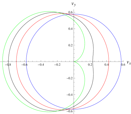
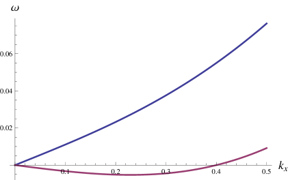
Figure 1: (Left) Sound velocity for $v=0$ (blue), $v=0.4$ (red), $v=0.6$ (black), $v=1/\sqrt{3}$ (green). (Right) Dispersion relation beyond the hydrodynamic limit for $v=0.5$ (blue) and $v=0.6$ (purple) and momentum in the direction of the superflow. The energy of the purple curve shows a minimum at finite momentum.

Going beyond the small momentum limit might give some insight on the fate of the superfluid after the instability is triggered. Indeed, as showed on the right hand side of Figure 1, for superflow velocities greater than $v^{*}$ the energy has a minimum at finite momentum, which signals an instability towards an inhomogeneous phase.

We have showed evidence for the existence of a phase transition to a non homogeneous phase at large enough superfluid velocities. In the next section we will address the issue of the construction of such a phase. The construction itself will show that the second order phase transition argued in this section is actually over-seeded by a first order phase transition at a smaller velocity.

2.3 Construction of the inhomogeneous phase

In this section we shall construct the inhomogeneous phase whose existence was hinted in the previous section. In order to do so we will add a spatial dependence to the ansatz for the fields that does not change the boundary conditions, so that the winding of the phase across the superfluid does not change. A natural way to do so is to add a periodic $x$ dependence.

To begin with, let us consider the following ansatz

$$\rho\equiv\rho(x)\,,$$ (18)

$$\psi\equiv-\mu\,t+\alpha(x)\,.$$ (19)

Let us expand $\rho(x)$ and $\alpha^{\prime}(x)$ alla Fourier

$$\rho(x)=\sum_{n=0}^{n_{max}}\rho_{n}\cos(nkx)\,,$$ (20)

$$\alpha^{\prime}(x)=\sum_{n=0}^{n_{max}}\alpha_{n}\cos(nkx)\,,$$ (21)

where $n_{max}$ will be a numerical cutoff and the zeroth coefficient gives the velocity $\alpha_{0}\equiv v$.

We can now use Mathematica’s FindRoot command to numerically integrate the equations of motion (5-6). The procedure consists in solving the equations for each Fourier mode up to a maximum $n_{max}$, chosen large enough so that we can trust that the solution won’t change significatively if further modes are taken into account. Two kind of solutions were found numerically. A first one in which all modes are null but the zero modes, and corresponds to the homogeneous phase. The second one is spatially modulated and the phase looks like a step function in the large $n_{max}$ limit. An example of both solutions can be observed in Figure 2

The picture would be the following. For certain critical velocity $v_{c}$ there is a first order phase transition. For low velocities $v<v_{c}$ the modulus of the condensate is constant and its phase is linear in $x$. As we increase the the velocity the phase at which the condensate is inhomogeneous dominates. In these solutions the phase of the order parameter is no longer linear with $x$, but a stairway of $v$ sized steps. Since there is no continuous connection between homogeneous and inhomogeneous solutions at finite $v$, the phase transition must be first order. Being that the case, the linear analysis of the previous section will not shed light on this phase transition.

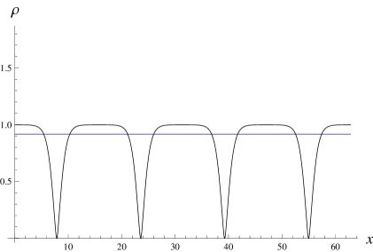
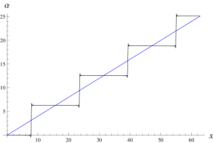
Figure 2: Modulus (left) and phase (right) for the homogeneous (blue) and inhomogeneous (black) solutions. This solutions correspond to $v=0.4$ and $n_{max}=60$.

In Figure 3 we plot the energy density of the homogeneous and inhomogeneous solutions. As we can see from the plot, the phase transition is indeed first order since the energy of the system (the energy of the solution with the lowest energy) has a discontinuity in its derivative, resulting from the fact that the inhomogeneous solution does not arise continuously from the homogeneous one. The critical velocity, where the energy of the different solutions is the same, is $v_{c}\approx 0.365<1/\sqrt{3}$. This first order phase transition overseeds the lineal instability of the homogeneous background, and the stability analysis should be redone considering fluctuations around this new background.

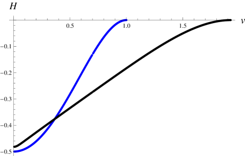
Figure 3: Energy density of the homogeneous (blue) and inhomogenous (black) solutions. We have used $n_{max}=60$ to generate this plot.

Another interesting fact that can be observed in Figure 3 is that while the homogeneous solutions with $\rho\neq 0$ only exist for $v<1$, inhomogeneous solutions exist for $v<\tilde{v}\approx 1.92$. The complete phase diagram would read as follows. For velocities larger than $\tilde{v}$ the system lives in the trivial solution, with no condensate. As we lower the velocity, a second order phase transition into the inhomogeneous solution occurs at $\tilde{v}$. If we keep on lowering the velocity a first order phase transition occur at $v_{c}$ into the homogenous phase. This phase dominates down to null velocity.

The existence of solutions with velocity larger than $v=1$ is very counterintuitive and may even seem unphysical but are certainly needed to smoothly connect with the normal phase. This should not be an issue since the phase uses the places in space to jump up to the next step precisely where the modulus $\rho$ is zero.Then we must analyze carefully the superfluid current

$$j_{\mu}=\rho(\partial_{\mu}\alpha+A_{\mu})\,,$$ (22)

which is a physical observable. When doing so we reach to the conclusion that even though the average velocity is grater than one, one can see that the supercurrent is time-like everywhere. Furthermore, $x$ component related to the flow is exactly zero everywhere since the phase is constant everywhere but in the places where the $\rho=0$. We reach then to the conclusion that for high enough superfluid velocities the system goes trough a first order phase transition into a static striped phase.

3 Inhomogeneous $U(2)$ superfluid

3.1 The model

Inspired by Kaon condensation in the color-flavor locked phase of QCD the authors of [18, 19] studied QCD at finite strangeness chemical potential. It was shown that at a critical chemical potential equal to the mass of the Kaons, Kaon condensation occurs through a continuous phase transition. Furthermore, a Goldstone boson with a non relativistic dispersion relation $\omega\sim p^{2}$ appears in the condensed phase spectrum. To illustrate such a fact the authors consider the following model:

$${\cal L}=-(\partial_{0}-i\mu)\phi^{\dagger}(\partial_{0}+i\mu)\phi+\partial_{i}\phi^{\dagger}\partial_{i}\phi+M^{2}\phi^{\dagger}\phi+\frac{\lambda}{2}(\phi^{\dagger}\phi)^{2}\,,$$ (23)

where $\phi$ is a complex scalar doublet,

$$\phi=\left(\begin{array}[]{c}\phi_{1}\\ \phi_{2}\end{array}\right).$$ (24)

Here we have introduced the chemical potential $\mu$ through an external gauge field, minimally coupled to the scalar doublet, following [18, 19].

While $\mu<M$ the masses of the four excitations of the theory are the roots $\omega$ of

$$(\omega\pm\mu)^{2}=M^{2}\,.$$ (25)

All of them are doubly degenerated. It is immediate to check that as soon as $\mu=M$ the $U(2)$ symmetry is broken and a new vacuum must be chosen:

$$\phi=\left(\begin{array}[]{c}0\\ \rho_{0}\end{array}\right),\qquad{\rm with}\quad\rho_{0}^{2}=\frac{\mu^{2}-M^{2}}{\lambda}\,.$$ (26)

If we study the fluctuations of $\phi$ around this background one finds two positive massive modes and two non massive modes with dispersion relations:

$$\omega_{1}^{2} =\frac{\mu^{2}-M^{2}}{3\mu^{2}-M^{2}}\,k^{2}+O(k^{4})\,,$$ (27)

$$\omega_{2}^{2} =6\mu^{2}-2M^{2}+O(k^{2})\,,$$ (28)

$$\omega_{3}^{2} =k^{2}-2\mu\omega_{3}\,,$$ (29)

$$\omega_{4}^{2} =k^{2}+2\mu\omega_{4}\,.$$ (30)

If we focus in the positive roots we see that $\omega_{1}$ is a normal Goldstone mode with a linear dispersion relation. The positive root of (29) is

$$\omega_{3}=\frac{k^{2}}{2\mu}+O(k^{4})\,.$$ (31)

This is by definition a type II Goldstone mode: it has a nonlinear dispersion relation proportional to an even power of momentum. Since the theory has Lorentz symmetry we also have a negative mode with quadratic dispersion. This comes from the negative root of $\omega_{3}$. Finally $\omega_{2}$ and $\omega_{4}$ are massive modes with

$$\omega_{4}=2\mu+O(k^{2})\,.$$ (32)

Since the symmetry breaking pattern is $U(2)\rightarrow U(1)$ we have three spontaneously broken generators but only two massless modes in the spectrum. This is due to the quadratic dispersion relation, and satisfies Chadha-Nielsen counting rules [20]. The role of $\omega_{4}$ is special since it is the mode that couples with the type II Goldstone mode in (29) and (30). There is evidence that its energy at zero momentum is protected under quantum corrections [25, 26, 27]. Some recent related papers are [21, 22, 23, 24].

As it has been pointed out in [17], the existence of this type II Goldstone modes should make the system unstable when an arbitrarily small velocity is turned on. We will address this issue more deeply.

3.2 Adding velocity naively

Let us naively add a velocity in the $x$ direction by turning on an external $A_{x}=v$ gauge field. Immediately we can see that this contributes to the condensate as a positive mass term, so the homogeneous classical solution will read

$$\phi=\left(\begin{array}[]{c}0\\ \rho_{0}\end{array}\right),\qquad{\rm with}\quad\rho_{0}^{2}=\frac{\mu^{2}-M^{2}-v^{2}}{\lambda}\,.$$ (33)

We shall consider again perturbations around this background. We can see that the lower sector is just that of the $U(1)$ sector studied previously, and will obviously show the same instabilities.

Now let us see what happens to the lower sector. We can see that the positive branch of the type II Goldstone now acquires a negative velocity

$$\omega_{3}=-\frac{vk_{x}}{\mu}+\frac{-(A_{x}\,k_{x})^{2}+\mu^{2}(k_{x}^{2}+k_{\bot}^{2})}{2\mu^{3}}+O(k^{4})\,.$$ (34)

This signals the fact that the energy minimum of the perturbation won’t be at zero momentum and that the system will rather be in a striped phase.

In order to make a more direct connection with the previous section we will go to the conformal limit where $M=0$, and we can choose $\lambda=1$. We will work at fixed chemical potential $\mu=1$, or equivalently we can say that we measure the velocity in terms of the chemical potential.

In figure 4 we can see the dispersion relation for the ex type II Goldstone mode $\omega_{3}$ plotted beyond the hydrodynamic limit, i.e. considering the expression (34) at all order in $k$. As we can see, as we increase the velocity the minimum in energy occurs at larger momentum. This hints a second order phase transition to an inhomogeneous phase as soon as we turn on a velocity.

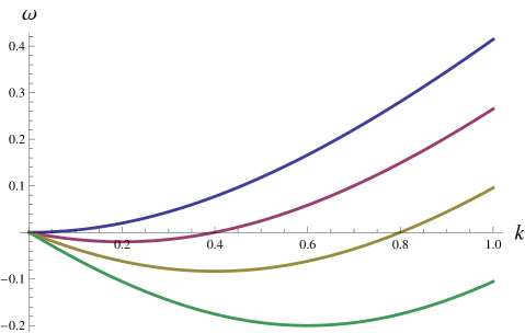
Figure 4: Dispersion relation of the type II Goldstone mode for $v=0$ (blue), $v=0.2$ (purple), $v=0.4$ (yellow) and $v=0.6$ (green).

We will repeat the mechanism of the previous section in order to construct inhomogeneous solutions corresponding to the $U(2)$ superfluid at finite velocity.

3.3 Constructing the inhomogeneous phase

In order to construct the inhomogeneous phase let us consider the following ansatz

$$\phi=\left(\begin{array}[]{c}\rho_{u}(x)e^{i\alpha_{u}(x)}\\ \rho_{d}(x)e^{i\alpha_{d}(x)}\end{array}\right)\,.$$ (35)

The classical equations of motions for the fields read

$$\rho_{u}^{\prime\prime} = \left(v+\alpha_{u}^{\prime}\right)^{2}\rho_{u}+(\rho_{d}^{2}+\rho_{u}^{2}-1)\rho_{u}\,,$$ (36)

$$0 = \rho_{u}\alpha_{u}^{\prime\prime}+2\left(v+\alpha_{u}^{\prime}\right)\rho_{u}^{\prime}\,,$$ (37)

$$\rho_{d}^{\prime\prime} = \left(v+\alpha_{d}^{\prime}\right)^{2}\rho_{d}+(\rho_{d}^{2}+\rho_{u}^{2}-1)\rho_{d}\,,$$ (38)

$$0 = \rho_{d}\alpha_{d}^{\prime\prime}+2\left(v+\alpha_{d}^{\prime}\right)\rho_{d}^{\prime}\,.$$ (39)

Again we will do a Fourier decomposition of the fields

$$\rho_{u}(x)=\sum_{n=0}^{n_{max}}\rho_{u}^{(n)}\cos(nkx)\,,$$ (40)

$$\alpha_{u}^{\prime}(x)=\sum_{n=1}^{n_{max}}\alpha_{u}^{(n)}\cos(nkx)\,,$$ (41)

$$\rho_{d}(x)=\sum_{n=0}^{n_{max}}\rho_{d}^{(n)}\cos(nkx)\,,$$ (42)

$$\alpha_{d}^{\prime}(x)=\sum_{n=1}^{n_{max}}\alpha_{d}^{(n)}\cos(nkx)\,,$$ (43)

where we have removed the zero modes of the phase since they will be taken into account in the spatial component of the external gauge field $A_{x}=v$.

We will now solve the equations for each Fourier mode numerically. Considering $\rho_{u}=0$ we recover the same solutions that in the previous section. When we allow a non-trivial profile for $\rho_{u}$ we find a further numerical solution. Its Fourier coefficients satisfy

$$\rho_{u}^{(n)}=(-1)^{n}\rho_{d}^{(n)},\quad\alpha_{u}^{(n)}=(-1)^{n}\alpha_{d}^{(n)}\,,$$ (44)

and correspond to a solution where both condensates are modulated, with a half period relative phase in their oscillatory space dependence. Their phases $\alpha_{u,d}$ are again step functions, and also have a half period relative phase. An example of these new solutions can be observed in Figure 5.

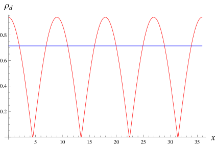
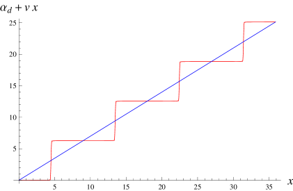
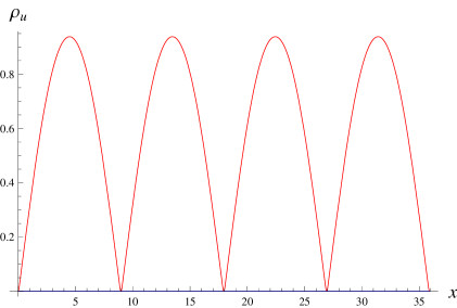
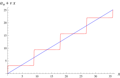
Figure 5: Homogeneous (blue) and inhomogeneous (red) solutions for $v=0.7$ and $n_{max}=60$.

In Figure 6 we show the energy density of this new configuration in contrast to the energy density of the solutions that also exist in the $U(1)$ model, i.e. the homogeneous solution and the solution with condensate in only one component. We can see that as soon as we turn on a velocity, a second order phase transition occurs into an inhomogeneous phase with two spatially modulated condensates. This is in agreement with the linear analysis done in Section 3.2. The order of the phase transition comes from the fact that the energy has the same slope for both solutions with respect to the velocity, which might be a bitt counter intuitive, since one solution does not emerge continuously from the other.

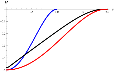
Figure 6: Energy density of the homogeneous (blue) and inhomogenous solutions with condensate only in the lower component (black) and with condensate in both components (red). We have used $n_{max}=40$ to generate this plot.

We can see from Figure 6 that the solution with two condensates always have the smallest free energy until it no longer exist at $\tilde{v}\approx 1.965$. At such critical velocity the superfluid solution is connected with the trivial solution.

Once again we can numerically check that the supercurrent is zero everywhere, so the system does not flow even though we turn on a superfluid velocity, but it develops stripes.

4 Conclusions

We have shown an example of a striped superfluid in a simple $\lambda\varphi^{4}$ model at finite velocity and chemical potential. We have studied two models one with global $U(1)$ gauge symmetry and the other one with $U(2)$.

For the $U(1)$ model the inhomogeneous solutions found are energetically favorable for large enough superfluid velocity. The homogeneous and inhomogeneous phases are connected via a first order phase transition. Increasing the velocity leads to a second order phase transition into a phase with no condensate. This work somehow completes the picture shown in [1, 2], about this very same model.

For the $U(2)$ model on the other hand, as soon as we turn on the velocity we end in a striped phase. This is in agreement with Landau criterion for superfluidity, since this model has zero velocity excitations. Increasing the velocity leads to a second order phase transition into a phase with no condensate.

As a possible continuation of this work, we would like to compute a similar computation in the context of AdS/CFT, following [6]. There, it is shown that the holographic $U(2)$ superfluid constructed in [28, 29] is unstable at all the range of velocities numerically reachable, while the $U(1)$ model of [5] is only unstable for large enough velocities, in agreement with the field theoretical predictions. The explicit construction of the holographic phases should be an interesting challenge.

Another interesting problem would be to analyze fluctuations around this inhomogeneous background, in order to address the problem of stability.

It would also be interesting to make a connection with fluids physics, looking at the hydrodynamic limit of this theory, following the steps of [1].

References

- [1] M. G. Alford, S. K. Mallavarapu, A. Schmitt and S. Stetina, “From a complex scalar field to the two-fluid picture of superfluidity,” Phys. Rev. D 87 (2013) 6, 065001 [arXiv:1212.0670 [hep-ph]].
- [2] M. G. Alford, S. K. Mallavarapu, A. Schmitt and S. Stetina, “Role reversal in first and second sound in a relativistic superfluid,” arXiv:1310.5953 [hep-ph].
- [3] S. A. Hartnoll, C. P. Herzog and G. T. Horowitz, “Building a Holographic Superconductor,” Phys. Rev. Lett. 101 (2008) 031601 [arXiv:0803.3295 [hep-th]].
- [4] P. Basu, A. Mukherjee and H. H. Shieh, “Supercurrent: Vector Hair for an AdS Black Hole,” Phys. Rev. D 79 (2009) 045010 [arXiv:0809.4494 [hep-th]].
- [5] C. P. Herzog, P. K. Kovtun and D. T. Son, “Holographic model of superfluidity,” Phys. Rev. D 79 (2009) 066002 [arXiv:0809.4870 [hep-th]].
- [6] I. Amado, D. Arean, A. Jimenez-Alba, K. Landsteiner, L. Melgar and I. S. Landea, “Holographic Superfluids and the Landau Criterion,” arXiv:1307.8100 [hep-th].
- [7] D. Arean, M. Bertolini, C. Krishnan and T. Prochazka, “Quantum Critical Superfluid Flows and Anisotropic Domain Walls,” JHEP 1109 (2011) 131 [arXiv:1106.1053 [hep-th]].
- [8] N. Jokela, G. Lifschytz and M. Lippert, “Flowing holographic anyonic superfluid,” arXiv:1407.3794 [hep-th].
- [9] V. I. Yukalov and E. P. Yukalova. “Stratification of moving multicomponent Bose-Einstein condensates.” Laser Physics Letters 1.1 (2004): 50. APA
- [10] M. Kunimi and Y. Kato. “Mean-field and stability analyses of two-dimensional flowing soft-core bosons modeling a supersolid.” Physical Review B 86.6 (2012): 060510.
- [11] P. F. Bedaque and T. Sch fer, “High density quark matter under stress,” Nucl. Phys. A 697 (2002) 802 [hep-ph/0105150].
- [12] C. Hoyos, B. S. Kim and Y. Oz, “Odd Parity Transport In Non-Abelian Superfluids From Symmetry Locking,” arXiv:1404.7507 [hep-th].
- [13] Z. Nussinov, “Avoided phase transitions and glassy dynamics in geometrically frustrated systems and non-Abelian theories,” Phys. Rev. B 69 (2004) 014208 [cond-mat/0209292].
- [14] L. Chayes, V. J. Emery, S. A. Kivelson, Z. Nussinov, and G. Tarjus, “Avoided critical behavior in a uniformly frustrated system,” Physica A 225(1) (1996), 129-153.
- [15] Z. Nussinov, “Commensurate and incommensurate O (n) spin systems: novel even-odd effects, a generalized Mermin-Wagner-Coleman theorem, and ground states,” [cond-mat/0105253].
- [16] S. Chakrabarty, Z. Nussinov, “Modulation and correlation lengths in systems with competing interactions,” Phys. Rev. B 84 (2011) 144402
- [17] G. E. Brown and M. Rho, “From chiral mean field to Walecka mean field and kaon condensation,” Nucl. Phys. A 596 (1996) 503 [nucl-th/9507028].
- [18] T. Schafer, D. T. Son, M. A. Stephanov, D. Toublan and J. J. M. Verbaarschot, “Kaon condensation and Goldstone’s theorem,” Phys. Lett. B 522 (2001) 67 [hep-ph/0108210].
- [19] V. A. Miransky and I. A. Shovkovy, “Spontaneous symmetry breaking with abnormal number of Nambu-Goldstone bosons and kaon condensate,” Phys. Rev. Lett. 88 (2002) 111601 [hep-ph/0108178].
- [20] H. B. Nielsen and S. Chadha, “On How to Count Goldstone Bosons,” Nucl. Phys. B 105 (1976) 445.
- [21] H. Watanabe and T. Brauner, “On the number of Nambu-Goldstone bosons and its relation to charge densities,” Phys. Rev. D 84 (2011) 125013 [arXiv:1109.6327 [hep-ph]].
- [22] H. Watanabe and H. Murayama, “Unified Description of Nambu-Goldstone Bosons without Lorentz Invariance,” Phys. Rev. Lett. 108 (2012) 251602 [arXiv:1203.0609 [hep-th]].
- [23] H. Watanabe and H. Murayama, “Redundancies in Nambu-Goldstone Bosons,” arXiv:1302.4800 [cond-mat.other].
- [24] Y. Hidaka, “Counting rule for Nambu-Goldstone modes in nonrelativistic systems,” Phys. Rev. Lett. 110 (2013) 091601 arXiv:1203.1494 [hep-th].
- [25] A. Kapustin, “Remarks on nonrelativistic Goldstone bosons,” arXiv:1207.0457 [hep-ph].
- [26] T. Brauner, “Spontaneous symmetry breaking in the linear sigma model at finite chemical potential: One-loop corrections,” Phys. Rev. D 74 (2006) 085010 [hep-ph/0607102].
- [27] A. Nicolis and F. Piazza, “A relativistic non-relativistic Goldstone theorem: gapped Goldstones at finite charge density,” Phys. Rev. Lett. 110 (2013) 011602 [arXiv:1204.1570 [hep-th]].
- [28] I. Amado, D. Arean, A. Jimenez-Alba, K. Landsteiner, L. Melgar and I. S. Landea, “Holographic Type II Goldstone bosons,” JHEP 1307 (2013) 108 [arXiv:1302.5641 [hep-th]].
- [29] A. Krikun, V. P. Kirilin and A. V. Sadofyev, “Holographic model of the multiband superconductor,” JHEP 1307 (2013) 136 [arXiv:1210.6074 [hep-th]].