DOCTOR OF PHILOSOPHY ASTROPHYSICS [Tenured Researcher INAOE, Mexico]Dr. Roberto Terlevich [Tenured Researcher INAOE, Mexico]Dr. Elena Terlevich [Tenured Researcher INAOE, Mexico & NOA, Greece]Dr. Manolis Plionis

Constraining the Parameter Space of the Dark Energy Equation of State Using Alternative Cosmic Tracers

To my parents, for their tireless support.

This dissertation is my own work and contains nothing which is the outcome of work done in collaboration with others, except as specified in the text and Acknowledgments.

I hereby declare that my thesis entitled:

Constraining the Parameter Space of the Dark Energy Equation of State Using Alternative Cosmic Tracers

is not substantially the same as any that I have submitted for a degree or diploma or other qualification at any other Research Institute or University.

Some parts of this work have already been published in refereed journals as follows:

• Section 3.3, H ii Galaxies as Cosmological Probes, has already partially appeared in Plionis et al. (2011).

• Chapter 4, The $L(\mathrm{H}\beta)-\sigma$ Relation for Massive Bursts of Star Formation, has already fully appeared in Chávez et al. (2014).

• Chapter 5, The Hubble Constant, has already partially appeared in Chávez et al. (2012).

I further declare that this copy is identical in every respect to the volume examined for the Degree, except that any alterations required by the Examiners have been made.

Date:

Signed:

Ricardo Chávez

We propose to use H ii galaxies to trace the redshift-distance relation, by means of their $L(\mathrm{H}\beta)-\sigma$ correlation, in an attempt to constrain the dark energy equation of state parameter solution space, as an alternative to the cosmological use of type Ia supernovae.

In order to use effectively high redshift H ii galaxies as probes of the dark energy equation of state parameter, we must reassess the $L(\mathrm{H}\beta)-\sigma$ distance estimator, minimising the observational uncertainties and taking care of the possible associated systematics, such as stellar age, gas metallicity, reddening, environment and morphology.

For a sample of 128 local ($0.02\lesssim z\lesssim 0.2$) compact H ii galaxies with high equivalent widths of their Balmer emission lines we obtained ionised gas velocity dispersion from high S/N, high-dispersion spectroscopy (Subaru-HDS and ESO VLT-UVES) and integrated H$\beta$ fluxes from low dispersion wide aperture spectrophotometry.

We find that the $L(\mathrm{H}\beta)-\sigma$ relation is strong and stable against restrictions in the sample (mostly based on the emission line profiles). The ‘gaussianity’ of the profile is important for reducing the rms uncertainty of the distance indicator, but at the expense of substantially reducing the sample. By fitting other physical parameters into the correlation we are able to significantly decrease the scatter without reducing the sample. The size of the starforming region is an important second parameter, while adding the emission line equivalent width or the continuum colour and metallicity, produces the solution with the smallest rms scatter, $\delta\log L(\mathrm{H}\beta)=0.233$.

We have used the $L(\mathrm{H}\beta)-\sigma$ relation from a local sample of H ii galaxies and a local calibration or ‘anchor’, given by giant H ii regions in nearby galaxies which have accurate distance measurements determined via primary indicators, to obtain a value of $H_{0}$. Using our best sample of 69 H ii galaxies (with $0.01<z<0.16$) and 23 Giant H ii regions in 9 galaxies we obtain $H_{0}=74.3\pm 3.1$ (statistical)$\pm$ 2.9 (systematic) km s^-1 Mpc^-1, in excellent agreement with, and independently confirming, the most recent SNa Ia based results.

Using a local sample (107 sources) and a sample of 21 high redshift H ii galaxies, 6 of them with medium-dispersion spectroscopy (ESO VLT-XShooter) and 17 taken from the literature, we have obtained constraints on the planes $H_{0}-\Omega_{m}$, $\Omega_{m}-w_{0}$ and $w_{0}-w_{1}$ (CPL model). Results are in line with other recent results although weaker due to the small size of the sample used. We expect to obtain better constraints using a larger high redshift sample.

Se propone el uso de la relación corrimiento al rojo - distancia de las galaxias H ii  mediada mediante el uso se su correlación $L(\mathrm{H}\beta)-\sigma$, con el fin de determinar la función de Hubble a corrimientos al rojo intermedios y altos, en un intento por restringir el espacio de soluciones de la ecuación de estado de la energía oscura, como una alternativa al uso de supernovas del tipo Ia (SNe Ia).

Con el fin de usar eficientemente a las galaxias H ii como trazadores cosmológicos, es necesario calibrar el estimador de distancia $L(\mathrm{H}\beta)-\sigma$, minimizando las incertidumbres observacionales e identificando los efectos sistemáticos asociados, tales como edad estelar, metalicidad del gas, enrojecimiento, medio ambiente y morfología.

Para una muestra local ($0.02\lesssim z\lesssim 0.2$) de 128 galaxias H ii compactas con altos anchos equivalentes en sus lineas de emisión de Balmer, se obtuvo la dispersión de velocidades del gas ionizado usando espectroscopía de alta dispersión y alta S/N (Subaru-HDS y ESO VLT-UVES) y flujos integrados de H$\beta$ usando espectro-fotometría de baja dispersión y apertura ancha.

Se encontró que la relación $L(\mathrm{H}\beta)-\sigma$  es resistente y estable ante restricciones en la muestra (basadas mayormente en los perfiles de las líneas de emisión). La ‘gaussianidad’ del perfil es importante para reducir la incertidumbre rms del indicador de distancia, pero a costa de una reducción substancial en el tamaño de la muestra. Ajustando otros parámetros físicos en la correlación, es posible reducir significativamente la dispersión sin reducir la muestra. El tamaño de la región de formación estelar es un importante segundo parámetro, mientras que agregando el ancho equivalente de las líneas de emisión o el color del continuo y la metalicidad, se encuentra la solución de menor dispersión rms, $\delta\log L(\mathrm{H}\beta)=0.233$.

Se ha usado el estimador $L(\mathrm{H}\beta)-\sigma$ de una muestra local de galaxias H ii y una calibración local o ‘ancla’ de esta correlación dada por regiones H ii gigantes en galaxias cercanas con mediciones de distancias precisas, determinadas mediante indicadores primarios, para obtener un valor de $H_{0}$. Usando la mejor muestra de 69 galaxias H ii  (con $0.01<z<0.16$) y 23 regiones H ii gigantes en 9 galaxias, se ha obtenido $H_{0}=74.3\pm 3.1$ (estadístico)$\pm$ 2.9 (sistemático) km s^-1 Mpc^-1, en excelente acuerdo con, y confirmando independientemente, los resultados mas recientes obtenidos con SNe Ia.

Usando una muestra local de 107 objetos y otra de 21 galaxias H ii a alto corrimiento al rojo, 6 de ellas con espectroscopía de mediana dispersión (ESO VLT-XShooter) y 17 tomadas de la literatura, se han obtenido restricciones en los planos $H_{0}-\Omega_{m}$, $\Omega_{m}-w_{0}$ y $w_{0}-w_{1}$ (modelo CPL). Los resultados están de acuerdo con otras determinaciones recientes aunque son más débiles. Se esperan obtener mejores restricciones con una muestra mas grande a alto corrimiento al rojo.

“Newton” by William Blake

The terms ‘cosmological constant’, ‘dark energy’ and ‘modified gravity’ have been remainders of our incomplete understanding of the “physical reality”. Our comprehension has been hampered by incomplete and biased data sets and the consequent theoretical over charged speculation.

Knowledge is constructed progressively, harsh and lengthy battles between proud theoretical systems, between judgements, must be fought before a glimpse of certainty can be acquired. However, sometimes an apparently tractable petit problem has been enough to demolish the noblest system.

The cosmic acceleration, detected at the end of the 1990s, could be one of this class of problems that are the key to a new view of reality. First of all, this problem is related to many fields in physics, crossing from gravitation to quantum field theory and to the unknown in the embodiment of quantum gravity with its multiple flavours (e.g. string theory, loop quantum gravity, twistor theory, …). Even more, the quest for a theoretical account of the observed acceleration has given an enormous impetus to the search for alternative theories of gravity.

The theoretical explanations for the cosmic acceleration are many and diverse, first of all we have the cosmological constant as a form of vacuum energy, then we are faced with a multitude of models in which its origin is explained by means of a substance with an exotic equation of state, and finally we encounter explanations based on modifications of the theory of general relativity.

The fact is that the current empirical data is not enough to discriminate between the great number of theoretical models, and therefore if we want to eventually decide on which is the best model we will need more and accurate data.

This work is devoted to explore the possibility of using H ii galaxies as probes for the cosmic expansion history. Many distinct probes already have been used or proposed, such as type Ia Supernovae, gamma ray bursts, baryon acoustic oscillations, galaxy clusters and weak lensing. From the previously mentioned only type Ia Supernovae, gamma ray bursts and H ii galaxies are purely geometrical probes (i.e. related directly to the metric), whereas the others are growth probes (i.e. related to the rate of growth of matter density perturbations) or a combination of both.

The advantage of using H ii galaxies over the use of type Ia Supernovae, as probes of cosmic acceleration, is that H ii galaxies can be observed easily to higher redshifts. Although, their distance modulus determinations, through their $L(\mathrm{H}\beta)-\sigma$ relation, have larger uncertainties than those of Supernovae Ia. Nevertheless, H ii galaxies would be a valuable complement to the type Ia Supernovae data, especially at high redshifts, and even more they could also be used as an independent confirmation for cosmic acceleration.

H ii galaxies are a promising new avenue for the determination of the cosmic expansion history. Their true value will be seen and assessed during coming years, when a large enough sample of intermediate and high redshift objects have been observed and analysed.

I wish to thank my advisors, Roberto Terlevich, Elena Terlevich and Manolis Plionis, for their constant support. I am truly grateful to them for their guidance and patience throughout these years of work. Their clear explanations and examples have many times helped me to make sense of obscure ideas.

I am also very grateful to Itziar Aretxaga, Mónica Rodríguez, Daniel Rosa-González, Divakara Mayya, Axel De La Macorra and Rafael Guzmán - Llorente my thesis evaluation committee and examiners, for undertaking the task of reviewing this manuscript and for their useful suggestions.

I am also very grateful to the staff at OAN, OAGH and NAOJ-Subaru for their help during our observing runs and to Elena Terlevich, Fabio Bresolin and Roberto Terlevich for their invaluable advice during our observations.

I also would like to thank to Jorge Melnick, Spyros Basilakos and Elias Koulouridis for their help and many useful observations during our collaborative work.

I would like to thank the CONACyT (Consejo Nacional de Ciencia y Tecnología). Without their scholarship (No. 224117), this thesis would not have been possible.

Last, but no least, I would like to thank my family and friends for their love and their help in finding my way through life. If it was not for their continuous support it would have been impossible for me to finish this work.

List of Symbols

We have attempted to keep the basic notation as standard as possible. In general, the notation is defined at its first occurrence in the text. The signature of the metric is assumed to be $(+,-,-,-)$ and the speed of light, $c$, is taken to be equal to $1$ throughout this work, unless otherwise specified. Throughout this work the Einstein summation convention is assumed. Note that throughout this thesis the subscript 0 denotes a parameter’s present epoch value, unless otherwise specified.

• The D’Alembert operator.

• The comoving distance.

• The Chi-square merit function.

• The perturbations to the mass-energy density decomposed into their Fourier modes.

• The metric connection coefficients or Christoffel symbols.

• The Einstein’s gravitational constant.

• The cosmological constant.

• The Lagrangian density or the likelihood estimator.

• The distance modulus.

• The mass-energy density nomarlized to the present $\rho_{c}$ value.

• The mass-energy density.

• The critical density (that required for the Universe to have a flat spatial geometry).

• The velocity dispersion from the emission-line width.

• The cosmic scale factor.

• The sound speed.

• The angular distance.

• The luminosity distance.

• The proper distance.

• The comoving volume element.

• The flux.

• The Einstein tensor.

• The metric.

• The Hubble parameter.

• The dimensionless Hubble parameter.

• The luminosity.

• The H ii galaxies distance indicator.

• The pressure.

• The deceleration parameter .

• The Ricci scalar.

• The Ricci tensor.

• The curvature radius.

• The core radius.

• The action.

• The scale of acoustic oscillations.

• The cosmological time.

• The stress-energy tensor.

• The line equivalent width.

• The equation of state parameter.

• The redshift.

Chapter 1 Introduction

“Begin at the beginning,” the King said gravely, “and go on till you come to the end: then stop.”

— L. Carroll, Alice in Wonderland

Our current understanding of the cosmological evidence shows that our Universe is homogeneous on the large-scale, spatially flat and in accelerated expansion; it is composed of baryons, some sort of cold dark matter and a component which acts as having a negative pressure (dubbed ’dark energy’ or ’cosmological constant’). The Universe underwent an inflationary infancy of extremely rapid growth, followed by a phase of gentler expansion driven initially by its relativistic and then by its non-relativistic contents but by now its evolution is governed by the dark energy component (e.g. Ratra & Vogeley, 2008; Frieman, Turner & Huterer, 2008).

The observational evidence for dark energy was presented in 1998 when two teams studying type Ia supernovae (SNe Ia), the Supernova Cosmology Project and the High-$z$ Supernova Search, found independently that these objects were further away than expected in a Universe without a cosmological constant (Riess et al., 1998; Perlmutter et al., 1999). Since then measurements of cosmic microwave background (CMB) anisotropy (e.g. Jaffe et al., 2001; Pryke et al., 2002; Spergel et al., 2007; Planck Collaboration et al., 2013) and of large-scale structure (LSS) (e.g. Tegmark et al., 2004; Seljak et al., 2005), in combination with independent Hubble relation measurements (Freedman et al., 2001), have confirmed the accelerated expansion of the Universe.

The accumulated evidence implies that nearly 70% of the total mass-energy of the Universe is composed of this mysterious dark energy; for which its nature is still largely unknown. Possible candidates of the cause of the accelerated expansion are Einstein’s cosmological constant, which implies that the dark energy component is constant in time and uniform in space (Carroll, 2001); or it could be that the dark energy is an exotic form of matter with a time dependent equation of state (e.g. Peebles & Ratra, 2003; Copeland, Sami & Tsujikawa, 2006); or since the range of validity of General Relativity (GR) is limited, an extended gravitational theory is needed (e.g. Joyce et al., 2014).

From the previous discussion we can see that understanding the nature of dark energy is of paramount importance and it could have deep implications for fundamental physics; it is thus of no surprise that this problem has been called out prominently in recent policy reports (Albrecht et al., 2006; Peacock et al., 2006) where extensive experimental programs to explore dark energy have been put forward.

To the present day, the cosmic acceleration has been traced directly only by means of SNe Ia and at redshifts, $z\sim 1$, a fact which implies that it is of great importance to use alternative geometrical probes at higher redshifts in order to verify the SNe Ia results and to obtain more stringent constrains in the cosmological parameters solution space, with the final aim of discriminating among the various theoretical alternatives that attempt to explain the accelerated expansion of the Universe (cf. Suyu et al., 2012).

1.1 Aims of this Work

The main objective of this work is to trace the Hubble function using the redshift-distance relation of H ii galaxies, as an alternative to SNe Ia, in an attempt to constrain the dark energy equation of state (Plionis et al., 2011). The main reasons for choosing H ii galaxies as alternative tracers of the Hubble function, are:

• H ii galaxies can be used as standard candles (Melnick, Terlevich & Terlevich, 2000; Melnick, 2003; Siegel et al., 2005; Plionis et al., 2011; Chávez et al., 2012) due to the correlation between their velocity dispersion and $\mathrm{H}\beta$-line luminosity (Terlevich & Melnick, 1981; Melnick, Terlevich & Moles, 1988; Chávez et al., 2014).

• H ii galaxies can be observed to higher redshifts than those sampled by current SNe Ia surveys and thus probe a region where the Hubble function is more sensitive to the cosmological parameter variations (Melnick, Terlevich & Terlevich, 2000; Plionis et al., 2011).

• The use of H ii galaxies as alternative high-$z$ tracer will enable us, to some extent, to independently verify the SNe Ia based results.

In order to use effectively high-$z$ H ii galaxies as geometrical probes, we need to locally re-assess the $L(\mathrm{H}\beta)-\sigma$ distance estimator, since this was originally done 30 years ago using non-linear detectors and without including corrections for effects such as the galaxy peculiar motions and environmental dependencies. Having this objective in mind, we must investigate, at low-$z$, all the parameters that can systematically affect the distance estimator; such as the stellar age, metallicity, extinction, environment, etc., with the intention to determine accurately the estimator’s zero-point.

After recalibration of the $L(\mathrm{H}\beta)-\sigma$ relation, we can use it to obtain luminosities for H ii galaxies to intermediate and high-$z$ and hence luminosity distances. Using a big enough sample it is possible to obtain as good or better constraints to $H_{0}$ and other cosmological parameters as currently obtained using SNe Ia (Plionis et al., 2011).

1.2 Structure of this Work

Through the second chapter we will be presenting the cosmic acceleration problem, its observational evidence, its implications and possible theoretical explanations and finally the possible avenues to constrain its parameters solution space in order to obtain a better understanding of its nature than currently known.

The third chapter explores the fundamental physical properties of H ii galaxies as young massive bursts of star formation and justifies their use as cosmological probe.

The fourth chapter explores the $L(\mathrm{H}\beta)-\sigma$ relation for H ii galaxies and its systematics such as stellar age, metallicity, extinction, environment, etc., with the intention of determining accurately the estimator’s slope.

Through the fifth chapter we apply the $L(\mathrm{H}\beta)-\sigma$ relation to the local determination of the Hubble parameter ($H_{0}$) and explore the related systematics. We analyse the $L(\mathrm{H}\beta)-\sigma$ relation for a sample of giant extragalactic H ii regions to accurately determine the correlation zero point, then using the already analysed H ii galaxies sample we determine the value of $H_{0}$.

In the sixth chapter we explore the application of the H ii galaxies $L(\mathrm{H}\beta)-\sigma$ relation to intermediate and high redshifts. We use a sample of 6 high redshift H ii galaxies observed using XShooter at the ESO-VLT combined with 17 objects taken from the literature to obtain constraints on the $H_{0}-\Omega_{m}$, $\Omega_{m}-w_{0}$ and $w_{0}-w_{1}$ planes.

Finally, in the seventh chapter we summarise the general conclusion to this work and the work to be done to improve the results already obtained.

Chapter 2 The Expanding Universe

We are to admit no more causes of natural things than such as are both true and sufficient to explain their appearances.

— I. Newton, Rules of Reasoning in Philosophy : Rule I

The current accepted cosmological model explains the history of the Universe as a succession of epochs characterised by their expansion rates. The Universe expansion rate has changed as one of its energy components dominates over all others. Near the beginning of time around $10^{-36}$ seconds after the ‘big bang’, the dominant component is the so called ‘inflaton’ field and the Universe expands exponentially, then after a reheating process, the dominant component is radiation followed by dark matter and at those epochs the expansion of the universe decelerates. Now the Universe is again in a phase of accelerated expansion and we call ‘dark energy’ the dominant component that causes it.

Our growing comprehension of the expanding Universe picture has advanced as new data has been accumulating through the technological improvements that have revolutionised astronomy during the past century. The first glimpse of the Universe expansion was obtained using ground based optical spectroscopy (Hubble, 1929), now the available data spans essentially all the electromagnetic spectrum, all kinds of astronomical techniques and is obtained through ground as well as space borne observations.

Through time different tracers have been used to measure the expansion rate, initially extragalactic Cepheids, now Supernovae Ia (SNe Ia), the Cosmic Microwave Background (CMB) and also galaxies. Even so, our current knowledge is insufficient to determine the nature of ‘dark energy’.

The cause of the cosmic acceleration is one of the most intriguing problems in all physics. In one form or another it is related to gravitation, high energy physics, extra dimensions, quantum field theory and even more exotic areas of physics, as quantum gravity or worm holes. However, we still know very little regarding the mechanism that drives the accelerated expansion of the Universe.

With the recent confirmation of the existence of the Higgs boson, the plot thickens even more. The electroweak phase transition generated by the Higgs potential induces a non vanishing contribution to the vacuum energy at the classical level that is blatantly in discordance with the accepted value for the cosmological constant in the ‘concordance’ ($\Lambda$CDM) cosmological model, thus leaving us with an embarrassingly large fine tuning problem (cf. Solà, 2013).

Due to the lack of a fundamental physical theory explaining the accelerated expansion, there have been many theoretical speculations about the nature of dark energy (e.g. Caldwell & Kamionkowski, 2009; Frieman, Turner & Huterer, 2008); furthermore and most importantly, the current observational/experimental data is not adequate to distinguish between the many adversary theoretical models.

Essentially one can probe dark energy by one or more of the following methods:

• Geometrical probes of the cosmic expansion, which are directly related to the metric like distances and volumes.

• Growth probes related to the growth rate of the matter density perturbations.

The existence of dark energy was first inferred from a geometrical probe, the redshift-distance relation of SNe Ia (Riess et al., 1998; Perlmutter et al., 1999); this method continues to be the preeminent way to probe directly the cosmic acceleration. The recent Union2.1 (Suzuki et al., 2012), SNLS3 (Conley et al., 2011) and PS1 (Rest et al., 2013) compilations of SNe Ia data are consistent with a cosmological constant, although the results, within reasonable statistical uncertainty, also agree with many dynamical dark-energy models (Shafer & Huterer, 2014). It is therefore of great importance to trace the Hubble function to higher redshifts than currently probed, since at higher redshifts the different models deviate significantly from each other (Plionis et al., 2011).

In this chapter we will explore the Cosmic Acceleration issue; the first section is devoted to a general account of the basics of theoretical and observational cosmology, in the second section we present a brief outlook of the observational evidence which supports the cosmic acceleration; later we will survey some of the theoretical explanations of the accelerating expansion and finally we will overview some probes used to test the Universe expansion.

Finally, a few words of caution regarding the terminology used. Through this chapter we will be using the term dark energy as opposed to cosmological constant, in the sense of a time-evolving cause of the cosmic acceleration. However, in later chapters we will use only the term dark energy since we consider it as the most general model, of which the cosmological constant is (mathematically) a particular case, while it effectively reproduces also the phenomenology of some modified gravity models.

2.1 Cosmology Basics

The fundamental assumption over which our current understanding of the Universe is constructed is known as the cosmological principle, which states that the Universe is homogeneous and isotropic on large-scales. The evidences that sustain the cosmological principle are basically the near-uniformity of the CMB temperature (e.g. Spergel et al., 2003) and the large-scale distribution of galaxies (e.g. Yadav et al., 2005).

Under the assumption of homogeneity and isotropy, the geometrical properties of space-time are described by the Friedmann-Robertson-Walker (FRW) metric (Robertson, 1935), given by

$$ds^{2}=dt^{2}-a^{2}(t)\left[\frac{dr^{2}}{1-kr^{2}}+r^{2}(d\theta^{2}+\sin^{2}\theta d\phi^{2})\right],$$ (2.1)

where $r$, $\theta$, $\phi$ are spatial comoving coordinates (i.e., where a freely falling particle comes to rest) and $t$ is the time parameter, whereas $a(t)$ is the cosmic scale factor which at the present epoch, $t_{0}$, has a value $a(t_{0})=1$; $k$ is the curvature of the space, such that $k=0$ corresponds to a spatially flat Universe, $k=1$ to a positive curvature (three-sphere) and $k=-1$ to a negative curvature (saddle as a 2-D analogue). Note that we are using units where the speed of light, $c=1$.

From the FRW metric we can derive the cosmological redshift, i.e. the amount that a photon’s wavelength ($\lambda$) increases due to the scaling of the photon’s energy with $a(t)$, with corresponding definition:

$$1+z\equiv\frac{\lambda_{0}}{\lambda_{e}}=\frac{a(t_{0})}{a(t)}=\frac{1}{a(t)},$$ (2.2)

where, $z$ is the redshift, $\lambda_{0}$ is the observer’s frame wavelength and $\lambda_{e}$ is the emission’s frame wavelength. Note that throughout this thesis the subscript 0 denotes a parameter’s present epoch value.

In order to determine the dynamics of the space-time geometry we must solve the GR field equations for the FRW metric, in the presence of matter, obtaining the cosmological field equations or Friedmann-Lemaître equations (for a full derivation see Appendix A):

$$\left(\frac{\dot{a}}{a}\right)^{2} = \frac{8\pi G\rho}{3}-\frac{k}{a^{2}}+\frac{\Lambda}{3},$$ (2.3)

$$\frac{\ddot{a}}{a} = -\frac{4\pi G}{3}(\rho+3p)+\frac{\Lambda}{3},$$ (2.4)

where $\rho$ is the total energy density of the Universe, $p$ is the total pressure and $\Lambda$ is the cosmological constant.

In eq.(2.3) we can define the Hubble parameter

$$H\equiv\frac{\dot{a}}{a},$$ (2.5)

of which its present value is conventionally expressed as $H_{0}=100h\ \mathrm{km\ s^{-1}\ Mpc^{-1}}$, where $h$ is the dimensionless Hubble parameter and unless otherwise stated we take a value of $h=0.743\pm 0.043$ (Chávez et al., 2012; Freedman et al., 2012; Riess et al., 2011; Freedman et al., 2001; Tegmark et al., 2006).

The time derivative of eq.(2.3) gives:

$$\ddot{a}=\frac{8\pi G}{3}\left(\rho a+\frac{\dot{\rho}a^{2}}{2\dot{a}}\right)+\frac{\Lambda a}{3},$$

and from the above and eq.(2.4) we can eliminate $\ddot{a}$ to obtain

$$\frac{-4\pi Ga}{3}\left[(\rho+3p)+2\left(\rho+\frac{\dot{\rho}a}{2\dot{a}}\right)\right] = 0$$

$$\frac{a}{\dot{a}}\dot{\rho}+3(\rho+p) = 0,$$

which then gives:

$$\dot{\rho}+\frac{3\dot{a}}{a}(\rho+p)=0,$$ (2.6)

which is an expression of energy conservation.

Equation (2.6) can be written as

$$\frac{d(\rho a^{3})}{dt} = -3a^{2}\dot{a}p$$ (2.7)

$$\frac{d(\rho a^{3})}{da} = -3a^{2}p,$$ (2.8)

and thus:

$$d(\rho_{i}a^{3})=-p_{i}da^{3},$$ (2.9)

where the subscript $i$ runs over all the components of the Universe. Equation (2.9) is the expanding universe analog of the first law of thermodynamics, $dE=-pdV$.

If we assume that the different components of the cosmological fluid have an equation of state of the generic form:

$$p_{i}=w_{i}\rho_{i},$$ (2.10)

then from eq.(2.8) we have

$$\frac{d(\rho_{i}a^{3})}{da}=-3w_{i}\rho_{i}a^{2},$$ (2.11)

which in the case where the equation of state parameter depends on time, ie., $w_{i}(a)$, the corresponding density takes the following form:

$$\rho_{i}\propto\exp\left\{-3\int{\frac{da}{a}[1+w_{i}(a)]}\right\}\;.$$ (2.12)

For the particular case where $w_{i}$ is a constant through cosmic time, we have

$$\rho_{i}\propto a^{-3(1+w_{i})},$$ (2.13)

where $w_{i}\equiv p_{i}/\rho_{i}$.These last two equations can be written as a function of redshift, defined by the eq.(2.2), as:

$$\rho_{i} \propto\exp{\left[3\int_{0}^{z}{\frac{1+w_{i}(z^{\prime})}{1+z^{\prime}}dz^{\prime}}\right]},$$ (2.14)

$$\rho_{i} \propto(1+z)^{3(1+w_{i})}\;.$$ (2.15)

For the case of non-relativistic matter (dark matter and baryons), $w_{m}=0$ and $\rho_{m}\propto(1+z)^{3}$, while for relativistic particles (radiation and neutrinos), $w_{r}=1/3$ and $\rho_{r}\propto(1+z)^{4}$, while for vacuum energy (cosmological constant), $w_{\Lambda}=-1$ and for which we have $p_{\Lambda}=-\rho_{\Lambda}=-\Lambda/8\pi G$.

In general the dark energy equation of state can be parameterized as (e.g. Plionis et al., 2009)

$$p_{w}=w(z)\rho_{w},$$ (2.16)

where

$$w(z)=w_{0}+w_{1}f(z),$$ (2.17)

with $w_{0}=w(0)$ and $f(z)$ is an increasing function of redshift, such as $f(z)=z/(1+z)$ (Chevallier & Polarski, 2001; Linder, 2003; Peebles & Ratra, 2003; Dicus & Repko, 2004; Wang & Mukherjee, 2006).

The so called critical density corresponds to the total energy density of the Universe. From eq.(2.3), where we take the cosmological constant as a cosmic fluid, and the definition of the Hubble parameter, eq.(2.5), we have that:

$$\rho_{c}\equiv\frac{3H_{0}^{2}}{8\pi G}=1.88\times 10^{-29}h^{2}\ \mathrm{g\ cm^{-3}}=8.10\times 10^{-47}h^{2}\ \mathrm{GeV^{4}}\;.$$ (2.18)

This parameter provides a convenient mean to normalize the mass-energy densities of the different cosmic components, and we can write:

$$\Omega_{i}=\frac{\rho_{i}(t_{0})}{\rho_{c}}\;,$$ (2.19)

where the subscript $i$ runs over all the different components of the cosmological fluid. Using this last definition and eq.(2.14) we can write eq.(2.3) as:

$$H^{2}(z)=H_{0}^{2}\left[\Omega_{r}(1+z)^{4}+\Omega_{m}(1+z)^{3}+\Omega_{k}(1+z)^{2}+\Omega_{w}\exp\left(3\int_{0}^{z}{\frac{1+w(z^{\prime})}{1+z^{\prime}}dz^{\prime}}\right)\right],$$ (2.20)

where $\Omega_{k}$ has been defined as

$$\Omega_{k}\equiv\frac{-k}{a^{2}H_{0}^{2}}\;.$$

By definition we have that $\Omega_{r}+\Omega_{m}+\Omega_{k}+\Omega_{w}\equiv 1$, and as a useful parameter we can define $\Omega_{0}\equiv\Omega_{r}+\Omega_{m}+\Omega_{w}$, such that for a positively curved Universe $\Omega_{0}>1$ and for a negatively curved Universe $\Omega_{0}<1$.

The value of the curvature radius, $R_{curv}\equiv a/\sqrt{|k|}$, is given by

$$R_{curv}=\frac{H_{0}^{-1}}{\sqrt{|\Omega_{0}-1|}},$$ (2.21)

then its characteristic scale or Hubble radius is given by $H_{0}^{-1}\approx 3000h^{-1}\ \mathrm{Mpc}$.

2.1.1 Observational toolkit

In observational cosmology the fundamental observable is the redshift, and therefore it is important to express the distance relations in terms of $z$. The first distance measure to be considered is the lookback time, i.e. the difference between the age of the Universe at observation $t_{0}$ and the age of the Universe, $t$, when the photons were emitted. From the definitions of redshift, eq.(2.2), and the Hubble parameter, eq.(2.5), we have:

$$\frac{dz}{dt}=-\frac{\dot{a}}{a^{2}}=-H(z)(1+z)\;,$$

from which we have:

$$dt=-\frac{dz}{H(z)(1+z)}\;,$$ (2.22)

and the lookback time is defined as:

$$t_{0}-t=\int_{t}^{t_{0}}{dt}=\int_{0}^{z}{\frac{dz^{\prime}}{H(z^{\prime})(1+z^{\prime})}}=\frac{1}{H_{0}}\int_{0}^{z}{\frac{dz^{\prime}}{(1+z^{\prime})E(z^{\prime})}}\;,$$ (2.23)

where

$$E(z)=\sqrt{\Omega_{r}(1+z)^{4}+\Omega_{m}(1+z)^{3}+\Omega_{k}(1+z)^{2}+\Omega_{w}\exp\left(3\int_{0}^{z}{\frac{1+w(z^{\prime})}{1+z^{\prime}}dz^{\prime}}\right)}\;.$$ (2.24)

From the definition of lookback time it is clear that the cosmological time or the time back to the Big Bang, is given by

$$t(z)=\int_{z}^{\infty}{\frac{dz^{\prime}}{(1+z^{\prime})H(z^{\prime})}}\;.$$ (2.25)

In the following discussion it will be useful to have an adequate parameterization of the FRW metric (Hobson, Efstathiou & Lasenby, 2005) which is given by:

$$ds^{2}=dt^{2}-a^{2}(t)\left[d\chi^{2}+S^{2}(\chi)(d\theta^{2}+\sin^{2}\theta d\phi^{2})\right],$$

where the function $r=S(\chi)$ is:

$$S(\chi)=\left\{\begin{array}[]{lc}\sqrt{k}^{-1}\sin(\chi\sqrt{k})&\mathrm{if}\ k>0,\\ \chi&\mathrm{if}\ k=0,\\ \sqrt{|k|}^{-1}\sinh(\chi\sqrt{|k|})&\mathrm{if}\ k<0,\\ \end{array}\right.$$ (2.26)

We can see that the comoving distance, i.e., that between two free falling particles which remains constant with epoch, is defined by:

$$\chi=\int_{t}^{t_{0}}{\frac{dt}{a(t)}}=\frac{1}{H_{0}}\int_{0}^{z}{\frac{dz^{\prime}}{E(z^{\prime})}}\;.$$ (2.27)

The transverse comoving distance (also called proper distance) is defined as:

$$D_{M}(t)=a(t)S(\chi),$$ (2.28)

At the present time and for the case of a flat model we have, $D_{M}=a(t_{0})\chi=\chi$.

The angular distance is defined as the ratio of an object’s physical transverse size to its angular size, and can be expressed as:

$$D_{A}=\frac{D_{M}}{1+z}\;.$$ (2.29)

Finally, the luminosity distance is defined by means of the relation

$$f=\frac{L}{4\pi D_{L}^{2}},$$ (2.30)

where $f$ is an observed flux, $L$ is the intrinsic luminosity of the observed object and $D_{L}$ is the luminosity distance; from which one obtains:

$$D_{L}=(1+z)D_{M}=(1+z)\int_{0}^{z}{\frac{dz^{\prime}}{H(z^{\prime})}}\;.$$ (2.31)

The distance modulus of a given cosmic object is defined as:

$$\mu\equiv m-M=5\log(D_{L}/10\ \rm{pc})$$ (2.32)

where $m$ and $M$ are the apparent and absolute magnitude of the object, respectively. If the distance, $D_{L}$, is expressed in Mpc then we have:

$$\mu=5\log D_{L}+25\;.$$ (2.33)

Through this relation and with the use of standard candles, i.e. objects of fixed absolute magnitude $M$, we can constrain the different parameters of the cosmological models via the construction of the Hubble diagram (the magnitude-redshift relation).

The following relation is useful when working with fluxes and luminosities instead of magnitudes,

$$\log L=\log f+0.4\mu+40.08\;,$$ (2.34)

where $f$ is the observed flux of the object, $L$ the luminosity and $\mu$ the distance modulus as defined in 2.33.

The scale factor can be Taylor expanded around its present value:

$$a(t) = a(t_{0})-(t_{0}-t)\dot{a}(t_{0})+\frac{1}{2}(t_{0}-t)^{2}\ddot{a}(t_{0})-\cdots$$

$$= a(t_{0})[1-(t_{0}-t)H(t_{0})-\frac{1}{2}(t_{0}-t)^{2}q(t_{0})H^{2}(t_{0})-\cdots]$$

$$= 1+H_{0}(t-t_{0})-\frac{1}{2}q_{0}H_{0}^{2}(t-t_{0})^{2}+\cdots\;,$$

where the deceleration parameter $q(t)$ is given by

$$q(t)\equiv-\frac{\ddot{a}(t)a(t)}{\dot{a}^{2}(t)}\;.$$ (2.35)

From the previous definitions we can write an approximation to the distance-redshift relation as

$$H_{0}D_{L}=z+\frac{1}{2}(1-q_{0})z^{2}+\cdots\;,$$ (2.36)

where we can recognize that for $z\ll 1$ it can be written as

$$H_{0}D_{L}\approx z,$$ (2.37)

which is known as the “Hubble law”.

Finally the comoving volume element, as a function of redshift, can be written as:

$$\frac{dV}{dzd\Omega}=\frac{S^{2}(\chi)}{H(z)}\;,$$ (2.38)

where $\Omega$ is the solid angle.

2.1.2 Growth of structure

The accelerated expansion of the Universe affects the evolution of cosmic structures since the expansion rate influences the growth rate of the density perturbations.

The basic assumptions regarding the evolution of structure in the Universe are that the dark matter is composed of non relativistic particles, i.e it is composed of what is called cold dark matter (CDM), and that the initial spectrum of density perturbations is nearly scale invariant, $P(k)\sim k^{n_{s}}$, where the spectral index is $n_{s}\simeq 1$, as it is predicted by inflation. With this in mind, the linear growth of small amplitude, matter density perturbations on length scales much smaller than the Hubble radius is governed by a second order differential equation, constructed by linearizing the perturbed equations of motions of a cosmic fluid element and given by:

$$\ddot{\delta_{k}}+2H\dot{\delta_{k}}-4\pi G\rho_{m}\delta_{k}=0,$$ (2.39)

where the perturbations $\delta_{k}\equiv\delta\rho_{m}(\mathbf{x},t)/\bar{\rho}_{m}(t)$ have been decomposed into their Fourier modes of wave number $k$. The expansion of the Universe enters through the so-called “Hubble drag” term, $2H\dot{\delta_{k}}$. Note that $\bar{\rho}_{m}$ is the mean density.

The growing mode solution of the previous differential equation, in the standard concordance cosmological model ($w_{\Lambda}=-1$) is given by:

$$\delta_{k}(z)\propto H(z)(5\Omega_{m}/2)\int_{z}^{\infty}{\frac{1+z^{\prime}}{H^{3}(z^{\prime})}dz^{\prime}}\;.$$ (2.40)

From the previous equation we obtain that, $\delta_{k}(t)$ is approximately constant during the radiation dominated epoch, grows as $a(t)$ during the matter dominated epoch and again is constant during the cosmic acceleration dominated epoch, in which the growth of linear perturbations effectively freezes.

2.2 Empirical Evidence

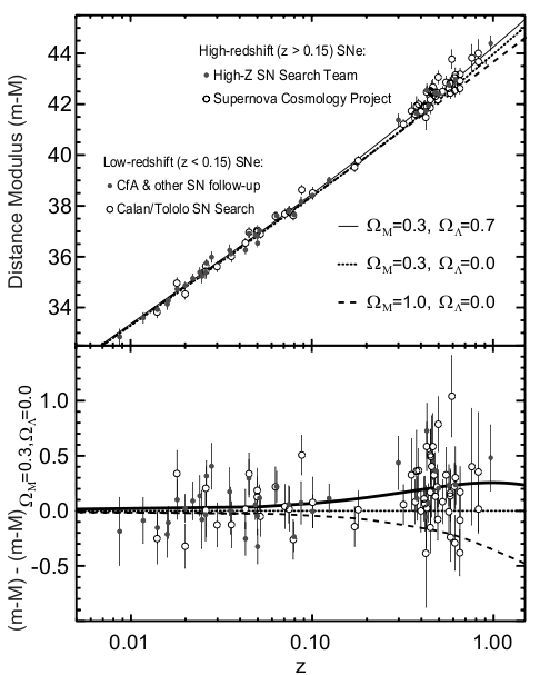
Figure 2.1: Upper panel: Hubble diagram of type Ia supernovae measured by the Supernova Cosmology Project and the High-z Supernova Team. Lower Panel: Residuals in distance modulus relative to an open Universe with $\Omega_{0}=\Omega_{m}=0.3$. Taken from Perlmutter & Schmidt (2003).

The cosmic acceleration was established empirically at the end of the 1990s when two independent teams, the Supernova Cosmology Project and the High-z Supernova Search, succeeded in their attempt to measure the supernova Hubble diagram up to relatively high redshifts ($z\sim 1$) (Riess et al., 1998; Perlmutter et al., 1999). Surprisingly, both teams found that the distant supernovae are $\sim 0.25\ \rm{mag}$ dimmer that they would be in a decelerating universe, indicating that the cosmic expansion has been accelerating over the past $\sim 7\ \mathrm{Gyr}$ (see Figure 2.1).

The cosmic acceleration has been verified by many other probes, and in this section we will briefly review the current evidence on which this picture of the Universe was constructed.

2.2.1 Cosmic microwave background

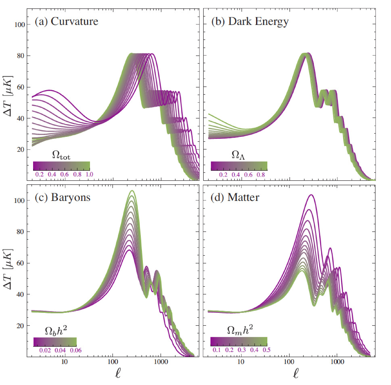
Figure 2.2: Sensitivity of the acoustic temperature spectrum to four fundamental cosmological parameters. (a) The curvature as quantified by $\Omega_{0}$. (b) The dark energy as quantified by the cosmological constant $\Omega_{\Lambda}$ ($w_{\Lambda}=-1$). (c) The baryon density $\Omega_{b}h^{2}$. (d) The matter density $\Omega_{m}h^{2}$. All parameters are varied around a fiducial model with: $\Omega_{0}=1,\Omega_{\Lambda}=0.65,\Omega_{b}h^{2}=0.02,\Omega_{m}h^{2}=0.147,n=1,z_{ri}=0,E_{i}=0$. Taken from Hu & Dodelson (2002).

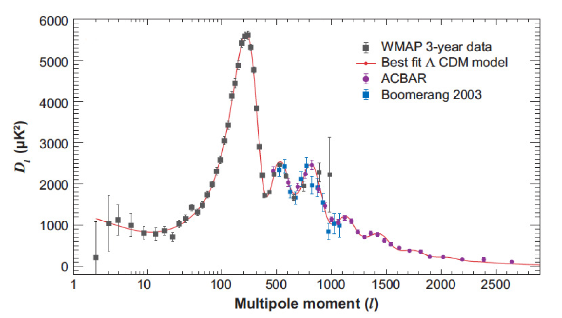
Figure 2.3: Angular power spectrum measurements of the cosmic microwave background temperature fluctuations from the Wilkinson Microwave Anisotropy Probe (WMAP), Boomerang, and the Arcminute Cosmology Bolometer Array Receiver (ACBAR). Taken from Frieman, Turner & Huterer (2008).

The measurement of the CMB black body spectrum was one of the most important tests of the big bang cosmology. The CMB spectrum started being studied by means of balloon and rocket borne observations and finally the black body shape of the spectrum was settled in the 1990s by observations with the FIRAS radiometer at the Cosmic Background Explorer Satellite (COBE) (Mather et al., 1990), which also showed that the departures from a pure blackbody were extremely small ($\delta E/E\leq 10^{-4}$) (Fixsen et al., 1996).

The CMB anisotropies provide a vision of the Universe when photons decoupled from baryons and before structure developed, about 380000 years after the Big Bang. The angular power spectrum of the CMB temperature anisotropies is dominated by acoustic peaks that arise from gravity-driven sound waves in the photon-baryon fluid. The position and amplitudes of the acoustic peaks indicate it the Universe is spatially flat or not (see Figure 2.2). Furthermore, in combination with Large Scale Structure (LSS) or independent $H_{0}$ measurements, it shows that the matter contributes only about 25% of the critical energy density (Hu & Dodelson, 2002). Clearly, a component of missing energy is necessary to match both results, a fact which is fully consistent with the dark energy being an explanation of the accelerated expansion.

Measurements of the angular power spectrum of the CMB have been carried out in the last ten years by many experiments (e.g. Jaffe et al., 2001; Pryke et al., 2002; Spergel et al., 2007; Reichardt et al., 2009)]. Figure 2.3 shows a combination of some recent results where the first acoustic peak around $l=200$ is clearly seen, which constrain the spatial curvature of the universe to be very close to null.

The most recent results from the Planck mission (Planck Collaboration et al., 2013) are shown in Figure 2.4. The Planck mission results are consistent with the standard spatially-flat six-parameter $\Lambda$CDM cosmology but with a slightly lower value for $H_{0}$ and a higher value for $\Omega_{m}$ compared with the SNe Ia results. When curvature is included, the Planck CMB data is consistent with a flat Universe to percent level precision.

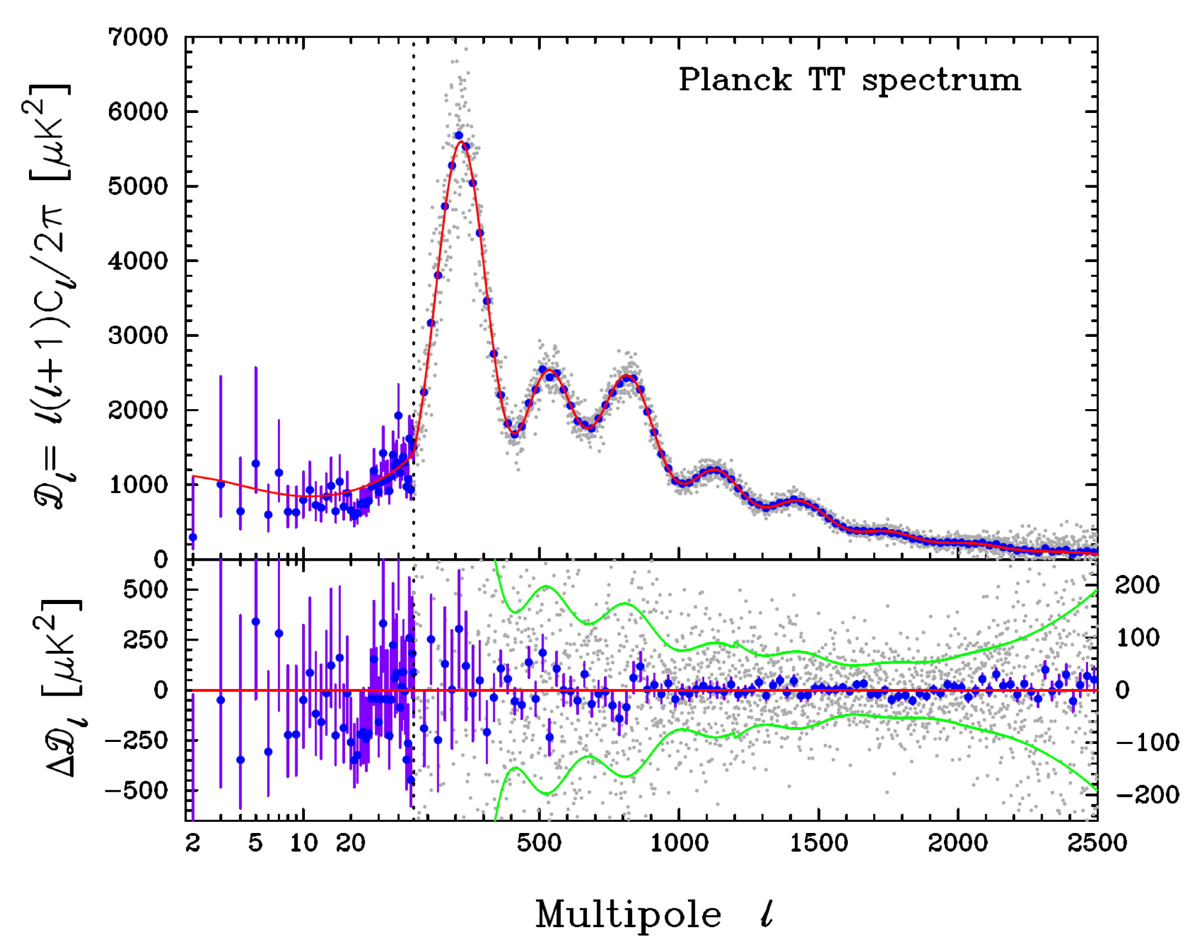
Figure 2.4: Angular power spectrum measurements of the cosmic microwave background temperature fluctuations form Planck. The power spectrum at low multipoles ($l=2-49$) is plotted in a logarithmic multipole scale. Taken from Planck Collaboration et al. (2013).

Although all these results are consistent with an accelerating expansion of the universe, they alone are not conclusive; other cosmological data, like the independent measurement of the Hubble constant, are necessary in order to indicate the cosmic acceleration.

2.2.2 Large-scale structure

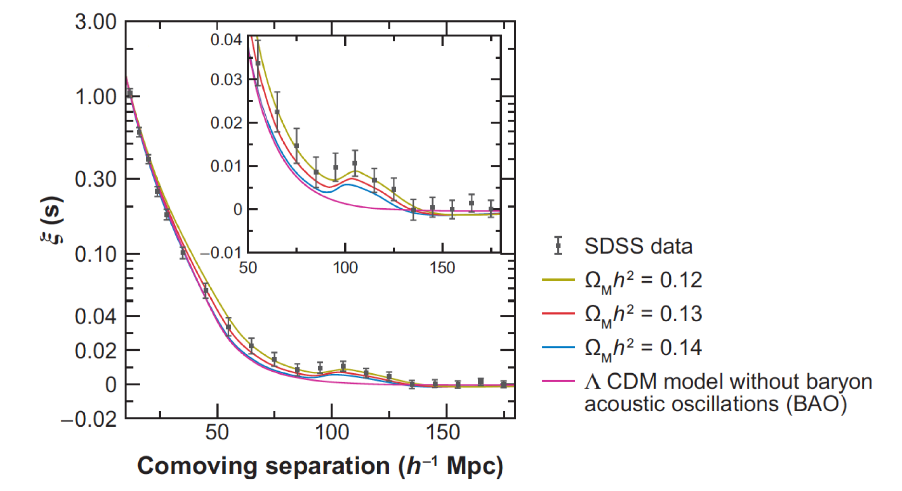
Figure 2.5: Detection of the baryon acoustic peak in the clustering of luminous red galaxies in the Sloan Digital Sky Survey (Eisenstein et al., 2005). The two-point galaxy correlation function in redshift space is shown; the inset shows an expanded view with a linear vertical axis. Curves correspond to the $\rm{\Lambda CDM}$ predictions for $\Omega_{m}h^{2}=0.12$ (dark yellow), $0.13$ (red), and $0.14$ (blue). The magenta curve shows a $\rm{\Lambda CDM}$ model without baryonic acoustic oscillations. Taken from Frieman, Turner & Huterer (2008).

The two-point correlation function of galaxies, as a measure of distribution of galaxies on large scales, has long been used to provide constrains on various cosmological parameters. The measurement of the correlation function of galaxies from the APM survey excluded, at that time, the standard cold dark matter (CDM) picture (Maddox et al., 1990) and subsequently argued in favor of a model with a low density CDM and possibly a cosmological constant (Efstathiou, Sutherland & Maddox, 1990).

The baryonic acoustic oscillations (BAO) leave a characteristic signature in the clustering of galaxies, a bump in the two-point correlation function at a scale $\sim 100h^{-1}\ \rm{Mpc}$ that can be measured today. Measurements of the BAO signature have been carried out by Eisenstein et al. (2005) for luminous red galaxies of the Sloan Digital Sky Survey (SDSS). They find results for the value of $\Omega_{m}h^{2}$ and the acoustic peak at $100h^{-1}\ \rm{Mpc}$ scale which are consistent with the outcome of the CMB fluctuation analyses (see Figure 2.5).

The recent work by Padmanabhan et al. (2012) reanalyses the Eisenstein et al. (2005) sample using an updated algorithm to account for the effects of survey geometry as well as redshift-space distortions finding similar results, while more recently Anderson et al. (2014), using the clustering of galaxies from the SDSS DR11 and in combination with the data from Planck find best fits of $\Omega_{m}h^{2}=0.1418\pm 0.0015$ and $\Omega_{m}=0.311\pm 0.009$.

2.2.3 Current supernovae results

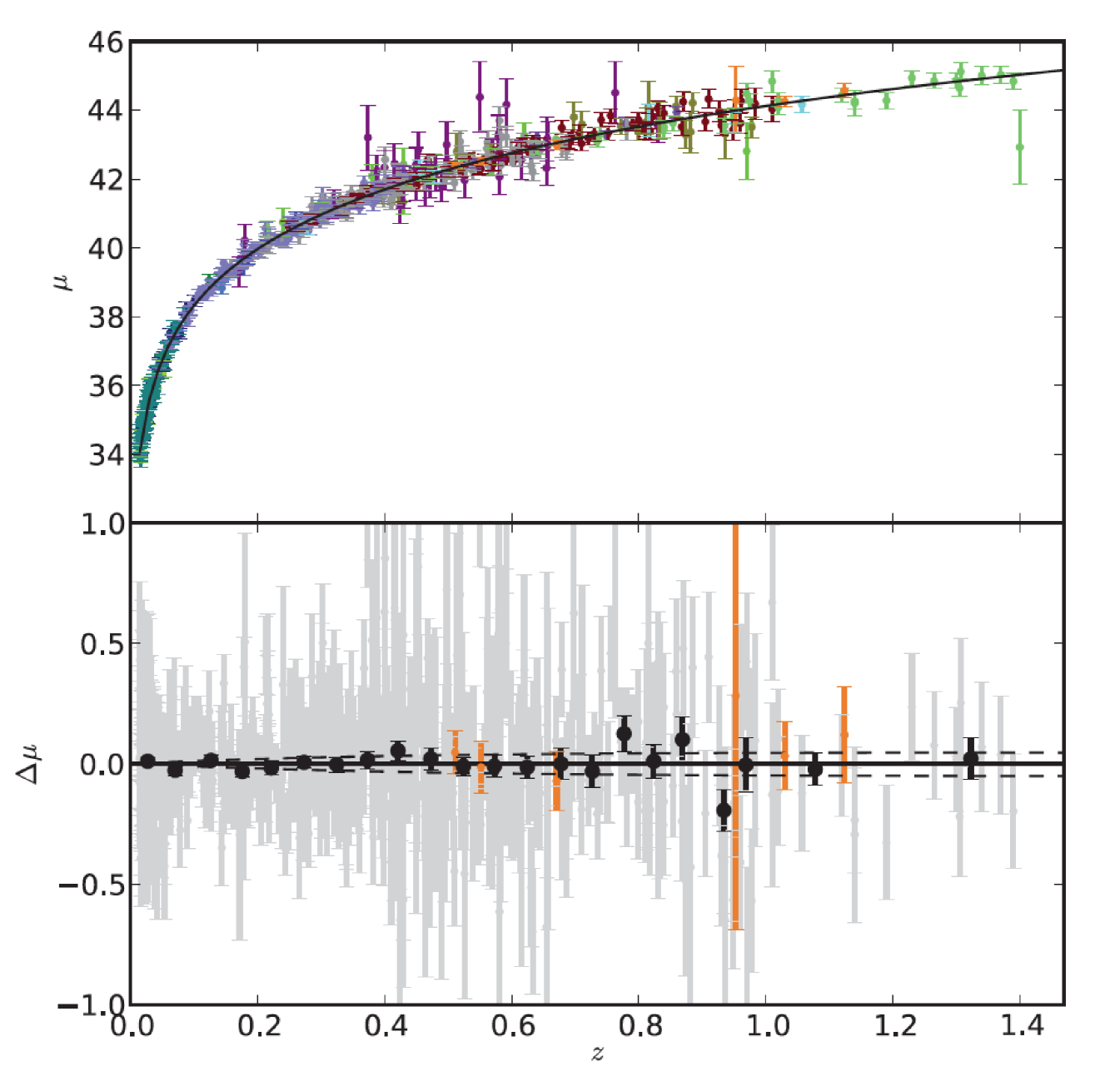
Figure 2.6: Upper panel: Hubble diagram for the Union2 SNe Ia compilation. The solid line represents the best fitted cosmology for a flat Universe including CMB and BAO constraints. The different colours indicate the different data. Lower panel: Hubble diagram residuals where the best fitted cosmology has been subtracted from the light curve shape and color corrected peak magnitudes. The grey points show the residuals for individual SNa, while the black points show the binned values in redshifts bins of $0.05$ for $z<1.0$ and $0.2$ for $z>1.0$. The dashed lines show the expected Hubble diagram residuals for cosmological models with $w\pm 0.1$ from the best fitted value. Taken from Amanullah et al. (2010).

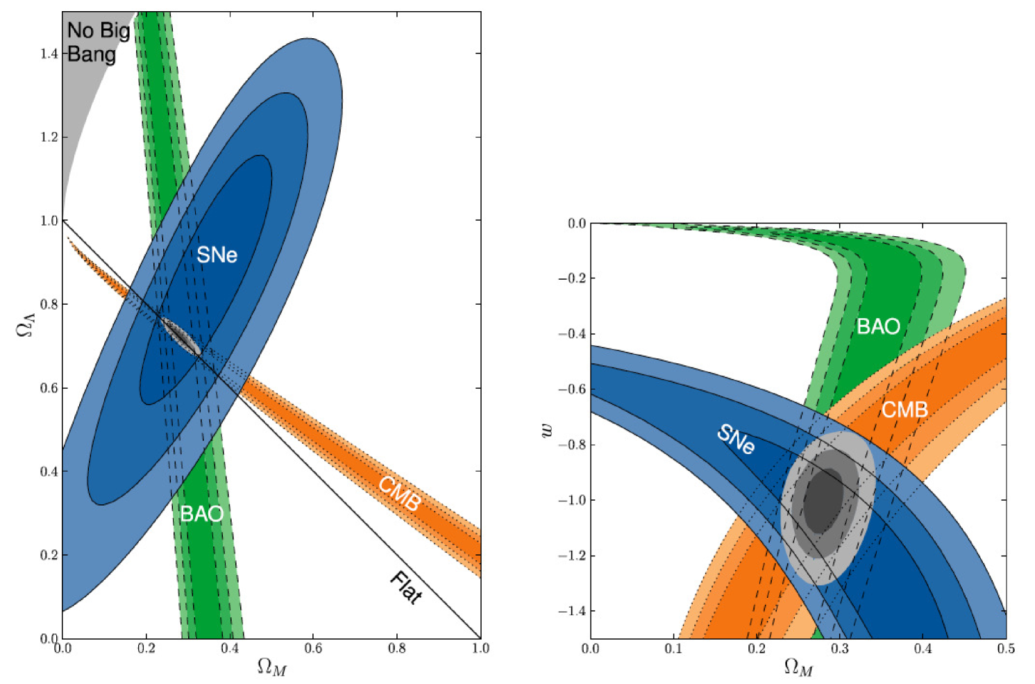
Figure 2.7: Left panel: 68.3 %, 95.4 % and 99.7% confidence regions in the ($\Omega_{m},\Omega_{\Lambda}$) plane from SNe, BAO and CMB with systematic errors. Cosmological constant dark energy ($w=-1$) has been assumed. Right panel: 68.3 %, 95.4 % and 99.7% confidence regions in the ($\Omega_{m},w$) plane from SNe, BAO and CMB with systematic errors. Zero curvature and constant $w$ has been assumed. Taken from Amanullah et al. (2010).

After the first SNe Ia results were published, concerns were raised about the possibility that intergalactic extinction or evolutionary effects could be the cause of the observed distant supernovae dimming (Aguirre, 1999; Drell, Loredo & Wasserman, 2000). Since then a number of surveys have been conducted which have strengthened the evidence for cosmic acceleration. Observations with the Hubble Space Telescope (HST), have provided high quality light curves (Riess et al., 2007), and observations with ground based telescopes, have permitted the construction of two large surveys, based on 4 meter class telescopes, the SNLS (Supernova Legacy Survey) (Astier et al., 2006) and the ESSENCE (Equation of State: Supernovae Trace Cosmic Expansion) survey (Miknaitis et al., 2007) with spectroscopic follow ups on larger telescopes.

The SNe Ia Hubble diagram has been constantly improved by the addition of new data, from the above mentioned surveys, mostly at $z<1.0$. Amanullah et al. (2010) have succeeded in analyzing the current SNe Ia data (557 objects) homogeneously and have taken care of known systematics, forming what has been named the Union2 compilation. Figure 2.6 shows the Hubble diagram based on the Union2 dataset, where the solid line represents the best fitted cosmology, obtained from an iterative $\chi^{2}$-minimization procedure based on:

$$\chi^{2}=\sum_{\rm{SNe}}{\frac{[\mu_{B}(\alpha,\beta,M_{B})-\mu(z;\Omega_{m},\Omega_{w},w)]^{2}}{\sigma_{\rm{ext}}^{2}+\sigma_{\rm{sys}}^{2}+\sigma_{\rm{lc}}^{2}}}\;,$$ (2.41)

where $\sigma_{\rm{lc}}$ is the propagated error of the covariance matrix of the light curve fit, whereas, $\sigma_{\rm{ext}}$ and $\sigma_{\rm{sys}}$ are the uncertainties associated with the Galactic extinction correction, host galaxy peculiar velocity and gravitational lensing, the former, and potential systematic errors the later. The observed distance modulus is defined as $\mu_{B}=m_{B}^{\mathrm{corr}}-M_{B}$, where $M_{B}$ is the absolute $B$-band magnitude and $m_{B}^{\mathrm{corr}}=m_{B}^{\mathrm{max}}+\alpha x_{1}-\beta c$; furthermore $m_{B}^{\mathrm{max}}$, $x_{1}$ and $c$ are parameters for each supernova that are weighted by the nuisance parameters $\alpha$, $\beta$ and $M_{B}$ which are fitted simultaneously with the cosmological parameters ($z;\Omega_{m},\Omega_{w},w$) which give the model distance modulus $\mu$.

Combining the data from the three probes that have been considered up to now, it is possible to obtain stronger constraints over the cosmological parameters (see Figure 2.7).

More recently, Suzuki et al. (2012) have added 23 SNe Ia (10 of which are beyond $z=1$) to the Union2 compilation to form the Union2.1 dataset. Using this improved catalog of SNe Ia jointly with BAO and CMB data they obtain even better constraints to the values of the cosmological parameters as shown in Table 2.1.

Table 2.1: $\chi^{2}$ minimisation results of cosmological parameters $\Omega_{m}$, $w$ and $\Omega_{k}$ and their uncertainties. Adapted from Suzuki et al. (2012).

Fit	$\Omega_{m}$	$\Omega_{k}$	$w$
SNe	$0.295^{+0.043}_{-0.040}$	$0$ (fixed)	$-1$ (fixed)
SNe + BAO + CMB	$0.286^{+0.018}_{-0.017}$	$-0.004^{+0.006}_{-0.007}$	$-1$ (fixed)
SNe + BAO + CMB + $H_{0}$	$0.272^{+0.015}_{-0.014}$	$0.002^{+0.007}_{-0.007}$	$-1.003^{+0.091}_{-0.095}$

2.3 Theoretical Landscape

The cosmic accelerated expansion has deep consequences for our understanding of the physical world. From the theoretical side many plausible explanations have been proposed. The “simplest” one is the traditional cosmological constant, but as we will see, this solution presents serious theoretical inconsistencies. To alleviate these problems various solutions have been proposed which involve either the introduction of an exotic fluid, with negative pressure, the dynamical consequences of which evolve with time (here we call them Dark Energy theories) or a modification of general relativity.

2.3.1 The cosmological constant

The Cosmological Constant, $\Lambda$, was introduced by Einstein in his field equations, in order to obtain a static solution. It is possible since the Einstein tensor, $G^{\mu\nu}=R^{\mu\nu}-1/2g^{\mu\nu}R$, satisfies the Bianchi identities $\nabla_{\nu}G^{\mu\nu}=0$ and the energy momentum tensor, $T^{\mu\nu}$, satisfies energy conservation $\nabla_{\nu}T^{\mu\nu}=0$; furthermore the metric, $g^{\mu\nu}$, is invariant to covariant derivatives $\nabla_{\alpha}g^{\mu\nu}=0$; then there is freedom to add a constant term to the GR equations:

$$R_{\mu\nu}-\frac{1}{2}g_{\mu\nu}R+\Lambda g_{\mu\nu}=8\pi GT_{\mu\nu}\;,$$ (2.42)

from which we can obtain equations (2.3) and (2.4). Form eq. (2.3) we can see that:

$$\rho_{\Lambda}=\frac{\Lambda}{8\pi G}\;,$$ (2.43)

and combining the above with eq.(2.4), we can see that $p_{\Lambda}=-\rho_{\Lambda}$. As an approximation, in the case in which the energy density of the cosmological constant dominates the dynamics of the Universe, and neglecting the matter component, we have that:

$$\frac{\ddot{a}}{a} =-\frac{4\pi G}{3}(\rho_{\Lambda}+3p_{\Lambda})$$

$$=\frac{8\pi G}{3}\rho_{\Lambda}\;.$$

From this rough argument, it becomes evident how the cosmological constant explains the phenomenology of the accelerated cosmic expansion, since it is clear that we have $\ddot{a}\propto\rho_{\Lambda}a$.

From the previous argument we see that for a cosmological constant we have $w=-1$. It is interesting to note that the current high-quality cosmological data strongly suggest that the mechanism behind the cosmic acceleration behaves exactly as a cosmological constant. However, we will show that the $\Lambda$-based explanation of the accelerating universe presents serious theoretical inconsistencies.

From the point of view of modern field theories, the cosmological constant can be explained as the energy of the vacuum. The possible sources for the vacuum energy are basically of two kinds: a bare cosmological constant in the general relativity action or the energy density of the quantum vacuum.

The cosmological constant problem

In this subsection we introduce the cosmological constant (cc) problem or the fine tuning problem that has a long history (Weinberg, 1989), the discussion is somewhat standard (Carroll, 2001) and we roughly follow the work of Solà (2013).

A bare cosmological constant ($\Lambda_{0}$) can be added in the Einstein-Hilbert (EH) action:

$$S_{EH}=\frac{-1}{16\pi G}\int{d^{4}x\sqrt{-g}(R+2\Lambda_{0})}=-\int{d^{4}x\sqrt{-g}\left(\frac{1}{16\pi G}R+\rho_{\Lambda_{0}}\right)}\;.$$ (2.44)

In fact this is the most general covariant action that we can construct from the metric and its first and second derivatives; we obtain eq.(2.42) varying this action with the addition of matter terms.

In the most simple case, the matter sector can be given by a single scalar field ($\phi$). In order to trigger Spontaneous Symmetry Breaking (SSB) and then preserve the gauge symmetry of the field, we must have a potential of the form:

$$V(\phi)=\frac{1}{2}m^{2}\phi^{2}+\frac{1}{4!}\lambda\phi^{4}\ (\lambda>0)\;,$$ (2.45)

where when $m^{2}>0$ we have a single vacuum state and $m$ plays the role of a mass for the free field, whereas when $m^{2}<0$ we have two degenerate vacuum states, this situation is characteristic of a phase transition.

The action for the gravitational system including $\phi$ can be given as:

$$S=S_{EH}+\int{d^{4}x\sqrt{\left\lvert g\right\rvert}\left[\frac{1}{2}g^{\mu\nu}\partial_{\mu}\phi\partial_{\nu}\phi-V(\phi)\right]}\;.$$ (2.46)

If we transfer the bare cc term to the matter sector then the matter action is given by,

$$S[\phi]=\int{d^{4}x\sqrt{\left\lvert g\right\rvert}\left[\frac{1}{2}g^{\mu\nu}\partial_{\mu}\phi\partial_{\nu}\phi-V(\phi)-\rho_{\Lambda_{0}}\right]}=\int{d^{4}x\sqrt{\left\lvert g\right\rvert}\mathcal{L}_{\phi}}\ \;.$$ (2.47)

Calculating the energy-momentum tensor for the matter Lagrangian, as defined above, we obtain,

$$\tilde{T}_{\mu\nu}^{\phi}=g_{\mu\nu}\rho_{\Lambda_{0}}+T_{\mu\nu}^{\phi}\;,$$ (2.48)

where $T_{\mu\nu}^{\phi}$ is the scalar field energy-momentum tensor given by

$$T_{\mu\nu}^{\phi}=\left[\partial_{\mu}\phi\partial_{\nu}\phi-\frac{1}{2}g_{\mu\nu}\partial_{\sigma}\phi\partial^{\sigma}\phi\right]+g_{\mu\nu}V(\phi)\;.$$ (2.49)

The vacuum expectation value for the ‘total’ energy-momentum tensor as given in eq. (2.48) is,

$$\langle\tilde{T}_{\mu\nu}^{\phi}\rangle=g_{\mu\nu}(\rho_{\Lambda_{0}}+\langle V(\phi)\rangle)\;,$$ (2.50)

where we note that the kinematical term in eq.(2.49) does not play any role.

As said above, SBB is present when $m^{2}<0$ and then the field vacuum expected value ($vev$) is not trivial and is given by,

$$\langle\phi\rangle=\sqrt{\frac{-6m^{2}}{\lambda}}\;,$$ (2.51)

and then the $vev$ for $V(\phi)$ is given by,

$$\rho_{\Lambda_{i}}=\langle V(\phi)\rangle=\frac{-3m^{4}}{2\lambda}=-\frac{1}{8}M_{H}^{2}\langle\phi\rangle^{2}=\frac{-1}{8\sqrt{2}}M^{2}_{H}M^{2}_{F}\;,$$ (2.52)

where we have introduced $M_{H}$, the physical mass of the Higgs boson, since this is just the process that happens (at the classical level) in the electroweak phase transition generated by the Higgs potential. The value of $M_{H}$ is given by,

$$M_{H}^{2}=\frac{\partial^{2}V(\phi)}{\partial\phi^{2}}\bigg{|}_{\phi=\langle\phi\rangle}=-2m^{2}>0\;.$$ (2.53)

Above, we also introduced the Fermi scale, $M_{F}=G^{-1/2}_{F}\simeq 293\ \mathrm{GeV}$. The value of $G_{F}$ is given by

$$\frac{G_{F}}{\sqrt{2}}=\frac{g^{2}}{8M^{2}_{W}}=\frac{1}{2\langle\phi\rangle}\;,$$ (2.54)

where $g$ is the weak gauge coupling and $M_{W}$ is the mass of the $W^{\pm}$ gauge boson. Then, we have a direct measure of the Higgs $vev$ given as:

$$\langle\phi\rangle=2^{-1/4}G^{-1/2}_{F}\simeq 246\ \mathrm{GeV}.$$ (2.55)

From eq.(2.50) it is clear that the $vev$ for $V(\phi)$ plays the role of an induced vacuum energy, hence we have identified it in this way in eq.(2.52). At this point the physical value of the cc is given by,

$$\rho_{\Lambda}=\rho_{\Lambda_{0}}+\rho_{\Lambda_{i}}\;.$$ (2.56)

At this stage, we already can compare the above calculations with observations, combining the results in eq.(2.55) and the recently measured value for $M_{H}\simeq 125\ \mathrm{GeV}$ (Aad et al., 2012), we obtain a value for $\rho_{\Lambda_{i}}\simeq-1.2\times 10^{8}\ \mathrm{GeV^{4}}$. The observed value of the cc is given by $\rho_{\Lambda}^{o}\sim 10^{-47}\ \mathrm{GeV^{4}}$, thus it is clear that,

$$\bigg{|}\frac{\rho_{\Lambda_{i}}}{\rho_{\Lambda}^{o}}\bigg{|}=\mathcal{O}(10^{55})\;.$$ (2.57)

The last result implies that we must choose the value of $\rho_{\Lambda_{0}}$ with a precision of 55 orders of magnitude in order to reconcile the above two results, which is clearly a severe fine-tuning problem.

The importance of the above result lies in the fact that the mass of the Higgs boson has been already measured and then at least in this, the simplest of cases, the reality of the vacuum energy density and hence the cc problem seems unavoidable.

In the most general case, and discussing the problem in a simplified way, the energy density of the quantum vacuum arises from the fact that for each mode of the quantum field there is a zero-point energy $\hbar\omega/2$. Formally the total energy would be infinite unless we discard the very high momentum modes on the ground that we trust the theory only to a certain ultraviolet momentum cutoff $k_{max}$, then we have

$$\rho_{\Lambda}=\frac{1}{2}\sum_{fields}{g_{i}\int_{0}^{\infty}{\frac{d^{3}k}{(2\pi)^{3}}\sqrt{k^{2}+m^{2}}}}\simeq\sum_{fields}{\frac{g_{i}k^{4}_{max}}{16\pi^{3}}},$$ (2.58)

where $g_{i}$ accounts for the degrees of freedom of the field (its sign is $+$ for bosons and $-$ for fermions). From the last equation we can see that $\rho_{\Lambda}\sim k^{4}_{max}$ , then imposing as a cutoff the energies where the known symmetry breaks, we have, in addition to the electroweak symmetry breaking discussed above, that:

• The potential arising from the breaking of chiral symmetry is due to the nonzero expectation value of the quark bilinear $q\bar{q}$ with a potential $M_{QCD}\sim 0.3\ \rm{GeV}$ and then its contribution to the vacuum energy is $\rho_{\Lambda}^{QCD}\sim(0.3\ \rm{GeV})^{4}\sim 1.6\times 10^{36}\ \rm{erg/cm^{3}}$.

• For the Planck scale transition we have a potential $M_{Pl}=(8\pi G)^{-1/2}\sim 10^{18}\ \rm{GeV}$ and then its contribution to the vacuum energy is $\rho_{\Lambda}^{Pl}\sim(10^{18}\ \rm{GeV})^{4}\sim 2\times 10^{110}\ \rm{erg/cm^{3}}$.

Then, the observed value of the vacuum energy density is $10^{55}-10^{120}$ times smaller than any theoretical prediction.

2.3.2 Dark energy theories

Due to the extreme fine tuning problem of the cc, several alternatives for the observed accelerated cosmic expansion have been proposed, a class of them postulates one or more dynamical fields with an effective value for the equation of state parameter, $w$, either different from $-1$ or changing with the redshift, in general they are called dark energy models. Over the years many different such models have been proposed, for a recent review see Copeland, Sami & Tsujikawa (2006).

In the dark energy approach the vacuum energy, arising from the ground states of the quantum fields, has a value exactly equal to zero due to e.g. some renormalization procedure. Then the cc problem does not arise at all.

The simplest dark energy proposal is a scalar field, in general this kind of models have been named quintessence. The action for this model is given by

$$S=\int{d^{4}x\sqrt{-g}\left(\frac{R}{16\pi G}+\mathcal{L}_{SM}+\mathcal{L}_{Q}\right)}\;,$$ (2.59)

where $R$ is the Ricci scalar, $g$ is the determinant of the metric, $\mathcal{L}_{SM}$ is the Lagrangian for Standard Model particles and the quintessence Lagrangian is given by

$$\mathcal{L}_{Q}=-\frac{1}{2}(\nabla_{\mu}Q)(\nabla^{\mu}Q)-V(Q)\;.$$ (2.60)

The field obeys the Klein-Gordon equation:

$$\Box Q=V_{,Q};$$ (2.61)

and its stress-energy tensor is given by

$$T_{\mu\nu}=(\nabla_{\mu}Q)(\nabla_{\nu}Q)+g_{\mu\nu}\mathcal{L}_{Q}\;,$$ (2.62)

with energy density and pressure given by:

$$\rho_{Q}=\frac{1}{2}\dot{Q}^{2}+V(Q), p_{Q}=\frac{1}{2}\dot{Q}^{2}-V(Q)\;.$$ (2.63)

Then its equation of state parameter, $w=p/\rho$, is given by:

$$w=\frac{\dot{Q}^{2}/2-V(Q)}{\dot{Q}^{2}/2+V(Q)}=\frac{-1+\dot{Q}^{2}/2V}{1+\dot{Q}^{2}/2V}\;,$$ (2.64)

from which it is obvious that if the evolution of the field is slow, we have $\dot{Q}^{2}/2V\ll 1$, and the field behaves like a slowly varying vacuum energy, with $w<0$, $\rho_{Q}(t)\propto V[Q(t)]$ and $p_{Q}(t)\propto-V[Q(t)]$.

2.3.3 Modified gravity theories

As it was mentioned earlier, an alternative explanation of the cosmic acceleration is through a modification to the laws of gravity. This implies a modification to the geometry side of the GR field equations, instead of the modification of the stress-energy tensor. Many ideas have been explored in this direction, some of them based on models motivated by higher-dimensional theories and string theory (e.g. Dvali, Gabadadze & Porrati, 2000; Deffayet, 2001) and others as phenomenological modifications to the Einstein-Hilbert action of GR (e.g. Carroll et al., 2004; Song, Hu & Sawicki, 2007).

2.4 Probes of Cosmic Acceleration

The accelerated expansion of the Universe appears to be a well established fact, while the dark energy density has been determined apparently to a precision of a few percent. However, measuring its equation of state parameter and determining if it is time-varying is a significantly more difficult task. The primary consequence of dark energy is its effect on the expansion rate of the universe and thus on the redshift-distance relation and on the growth-rate of cosmic structures. Therefore, we have basically two kinds of probes for dark energy, one geometrical and the other one based on the rate of growth of density perturbations.

The Growth probes are related to the rate of growth of matter density perturbations, a typical example being the spatial clustering of extragalactic sources and its evolution (e.g. Pouri, Basilakos & Plionis, 2014). The Geometrical probes are related directly to the metric, a typical example being the redshift-distance relation as traced by SNe Ia (e.g. Suzuki et al., 2012).

In general, in order to use the latter probes, based on any kind of tracers, one has to measure the redshift which is relatively straightforward, but also the tracer distance, which in general is quite difficult. In Appendix B we review the cosmic distance ladder which allows the determination of distances to remote sources.

2.4.1 Type Ia supernovae

Type Ia Supernovae have been used as geometrical probes, they are standard candles (Leibundgut, 2001), which through their determination of the Hubble function have provided constrains of cosmological parameters through eq.(2.32). Up to date they are the most effective, and better understood, probe of the cosmic acceleration (Frieman, Turner & Huterer, 2008).

The standardisation of SNe Ia became possible after the work of Phillips (1993) where an empirical correlation was established between their peak brightness and the luminosity decline rate, after peak luminosity (in the sense that more luminous SNe Ia decline more slowly).

The main systematics in the distance determination derived from SNe Ia, are uncertainties in host galaxy extinction correction and in the SNe Ia intrinsic colours, luminosity evolution and selection bias in the low redshift samples (Frieman, Turner & Huterer, 2008). The extinction correction is particularly difficult since having the combination of photometric errors, variation in intrinsic colours and host galaxy dust properties, causes distance uncertainties even when using multiband observations. However, a promising solution to this problem is based on near infrared observations, where the extinction effects are significantly reduced.

Frieman et al. (2003) estimated that in order to obtain precise measurements of $w_{0}$ and $w_{1}$, accounting for SNe Ia systematics, requires $\sim 3000$ light curves out to $z\sim 1.5$, measured with great precision and careful control of the systematics.

2.4.2 Galaxy clusters

The utility of galaxy clusters as cosmological probes relies in many aspects, among which is the determination of their mass to light ratio, where its comparison with the corresponding cosmic ratio can provide the value of $\Omega_{m}$ (e.g. Andernach et al., 2005), the cluster masses can be also used to derive the cluster mass function to be compared with the analytic (Press-Schechter) or numerical (N-body simulations) model expectations (Basilakos, Plionis & Solà, 2009; Haiman, Mohr & Holder, 2001; Warren et al., 2006). The determination of the cluster mass can be done by means of the relation between mass and other observable, such as X-ray luminosity or temperature, cluster galaxy richness, Sunyaev-Zel’dovich effect (SZE) flux decrement or weak lensing shear, etc (Frieman, Turner & Huterer, 2008).

Frieman, Turner & Huterer (2008) give the redshift distribution of clusters selected according to some observable $O$, with selection function $f(O,z)$ as

$$\frac{d^{2}N(z)}{dzd\Omega}=\frac{r^{2}(z)}{H(z)}\int_{0}^{\infty}{f(O,z)dO}\int_{0}^{\infty}{p(O|M,z)\frac{dn(z)}{dM}dM}\;,$$ (2.65)

where $dn(z)/dM$ is the space density of dark halos in comoving coordinates and $p(O|M,z)$ is the mass-observable relation, the probability that a halo of mass $M$, at redshift $z$, is observed as a cluster with observable property $O$. We can see that this last equation depends on the cosmological parameters through the comoving volume element (see equation (2.38)) and the term $dn(z)/dM$ which depends on the evolution of density perturbations.

2.4.3 Baryon acoustic oscillations

Gravity drives acoustic oscillations of the coupled photon-baryon fluid in the early universe. The scale of the oscillations is given by

$$s=\int_{0}^{t_{rec}}{c_{s}(1+z)dt}=\int_{z_{rec}}^{\infty}{\frac{c_{s}}{H(z)}dz},$$ (2.66)

where $c_{s}$ is the sound speed which is determined by the ratio of the baryon and photon energy densities, whereas $t_{rec}$ and $z_{rec}$ are the time and redshift when recombination occurred. These acoustic oscillations leave their imprint on the CMB temperature anisotropy angular power spectrum but also in the baryon mass-density distribution. From the WMAP measurements we have $s=147\pm 2\ \mathrm{Mpc}$. Since the oscillations scale $s$ provides a standard ruler that can be calibrated by the CMB anisotropies, then measurements of the BAO scale in the galaxy distribution provides a geometrical probe for cosmic acceleration (Frieman, Turner & Huterer, 2008).

The systematics that could affect the BAO measurements are related to nonlinear gravitational evolution effects, scale-dependent differences between the clustering of galaxies and of dark matter (the so-called bias) and redshift-space distortions of the clustering, which can shift the BAO features (Frieman, Turner & Huterer, 2008).

2.4.4 Weak gravitational lensing

The images of distant galaxies are distorted by the gravitational potential of foreground collapsed structures, intervening in the line of sight of the distant galaxies. This distortion can be used to measure the distribution of dark matter of the intervening structures and its evolution with time, hence it provides a probe for the effects of the accelerated expansion on the growth of structure (Frieman, Turner & Huterer, 2008).

The gravitational lensing produced by the large scale structure (LSS) can be analysed statistically by locally averaging the shapes of large numbers of distant galaxies, thus obtaining the so called cosmic shear field at any point. The angular power spectrum of shear is a statistical measure of the power spectrum of density perturbations, and is given by (Hu & Jain, 2004):

$$P^{\gamma}_{l}(z_{s})=\int_{0}^{z_{s}}{dz\frac{H(z)}{D^{2}_{A}(z)}|W(z,z_{s})|^{2}P_{\rho}\left(k=\frac{l}{D_{A}(z)};z\right)},$$ (2.67)

where $l$ is the angular multipole of the spherical harmonic expansion, $W(z,z_{s})$ is the lensing efficiency of a population of source galaxies and it is determined by the distance distributions of the source and lens galaxies, and $P_{\rho}(k,z)$ is the power spectrum of density perturbations.

Some systematics that could affect weak lensing measurements are, obviously, incorrect shear estimates, uncertainties in the galaxy photometric redshift estimates (which are commonly used), intrinsic correlations of galaxy shapes and theoretical uncertainties in the mass power spectrum on small scales (Frieman, Turner & Huterer, 2008).

2.4.5 H ii galaxies

H ii galaxies are dwarf galaxies with a strong burst of star formation which dominates the luminosity of the host galaxy and allows it to be seen at very large distances. The $L(\mathrm{H}\beta)-\sigma$ relation of H ii galaxies allows distance modulus determination for these objects and therefore the construction of the Hubble diagrams. Hence, H ii galaxies can be used as geometrical probes of the cosmic acceleration.

Previous analyses (Terlevich & Melnick, 1981; Melnick et al., 1987), have shown that the H ii galaxy oxygen abundance affects systematically its $L(\mathrm{H}\beta)-\sigma$ relation. The distance indicator proposed by the authors takes into account such effects (Melnick, Terlevich & Moles, 1988), and was defined as:

$$M_{z}=\frac{\sigma^{5}}{\mathrm{O/H}}\;,$$ (2.68)

where $\sigma$ is the galaxy velocity dispersion and $\mathrm{O/H}$ is the oxygen abundance relative to hydrogen. From this distance indicator, the distance modulus can be calculated as: (Melnick, Terlevich & Terlevich, 2000)

$$\mu=2.5\log_{10}\frac{\sigma^{5}}{F(\rm{H}\beta)}-2.5\log_{10}(\rm{O/H})-A_{\rm{H}\beta}-26.44,$$ (2.69)

where $F(\rm{H}\beta)$ is the observed $\rm{H}\beta$ flux and $A_{\rm{H}\beta}$ is the total extinction in $H\beta$.

Some possible systematics that could affect the $L(\mathrm{H}\beta)-\sigma$ relation, are related to the reddening, the age of the stellar burst, as well as the local environment and morphology.

Through the next chapter we will explore carefully the use of H ii galaxies as tracers of the Hubble function and the systematics that could arise when calibrating the $L(\mathrm{H}\beta)-\sigma$ relation for these objects.

2.5 Summary

The observational evidence for the Universe accelerated expansion is now overwhelming. The best to date data from SNe Ia, BAOs, CMB and many other tracers, all accord that we are living during an epoch in which the evolution of the Universe is dominated by some sort of dark energy.

Many different models have been proposed to explain the observed dark energy. The cosmological constant is a good candidate in the sense that all current observations are consistent with it, although suffers from severe fine tuning and coincidence problems that have given place to the proposal of dynamical vacuum energy models.

In this work we will explore an alternative probe to trace the expansion history of the Universe. H ii galaxies are a promising new way to explore the nature of dark energy since they can be observed to larger redshifts that many of the currently best known cosmological probes.

Chapter 3 H ii Galaxies

                                                 Pauca sed matura.

— C.F. Gauss, Motto

In the search for white dwarfs, Humason & Zwicky (1947), using the 18 inch Schmidt telescope at Palomar, developed the technique of using multiply exposed large scale plates, each exposure covering a distinct region of the optical spectrum with the intention of identifying the target objects from the relative intensities in the different plates.

Haro (1956), while searching for emission line galaxies, using a variation of the technique pioneered by Humason and Zwicky (using an objective prism), discovered some compact galaxies with strong emission lines. Some years later Sargent & Searle (1970) found in what was to become the Zwicky & Zwicky (1971) catalogue, some compact galaxies whose spectra were very similar to those of giant H ii regions in spiral galaxies. They called them isolated extragalactic H ii regions. After analysing their spectra they conclude that the galaxies are ionised by massive clusters of OB stars (Searle & Sargent, 1972; Bergeron, 1977) and are metal poor systems (Searle & Sargent, 1972; Lequeux et al., 1979; French, 1980; Kunth & Sargent, 1983).

Since H ii galaxies were easily recognised in objective prism plates, due to their strong narrow emission lines, many were discovered by objective prism surveys during the following years (Markarian, 1967; Smith, Aguirre & Zemelman, 1976; MacAlpine, Smith & Lewis, 1977; Markarian, Lipovetskii & Stepanyan, 1981).

Terlevich & Melnick (1981) and Melnick, Terlevich & Moles (1988) analysed the dynamical properties of H ii galaxies and proposed their usefulness as distance indicators; the data used for their analysis was published subsequently as a spectrophotometric catalogue (Terlevich et al., 1991) that has been used since in H ii galaxies research.

Throughout the first section of the current chapter we will explore the main properties of H ii galaxies, then we will discuss their $L(\mathrm{H}\beta)-\sigma$ relation and their possible systematics, ending with an analysis of their use to constraint the dark energy equation of state parameters.

3.1 H ii Galaxies Properties

3.1.1 Giant extragalactic H ii regions and H ii galaxies

One of the defining characteristics of both H ii galaxies and Giant Extragalactic H ii Regions (GEHRs), is that the turbulent motions of their gaseous component are supersonic (Melnick et al., 1987).

GEHRs are zones of intense star formation in late type spirals (Sc) and irregular galaxies. Ionising photons are generated by clusters of OB stars at a rate of $10^{51}-10^{52}\ \mathrm{s^{-1}}$, ionising large amounts ($10^{4}-10^{6}\ \mathrm{M_{\odot}}$) of low density ($N_{e}\approx 10-100\ \mathrm{cm^{-3}}$), inhomogeneously distributed gas. GEHRs have typical dimensions of the order $10^{2}-10^{3}\ \mathrm{pc}$ and diverse morphologies (Shields, 1990; García-Benito, 2009).

H ii galaxies are dwarf starforming galaxies that have undergone a recent episode of star formation, and their interstellar gas is ionised by one or more massive clusters of OB stars. This type of galaxies have total masses of less than $10^{11}\ \mathrm{M_{\odot}}$ and a radius of less than $2\ \mathrm{kpc}$ with a surface brightness $\mu_{V}\geq 19\ \mathrm{mag\ arcsec^{-2}}$ (García-Benito, 2009).

H ii galaxies, being active starforming dwarf galaxies, are also a subset of the blue compact dwarf (BCD) galaxies, although in general the term “H ii galaxy” is used when the objects have been selected for their strong, narrow emission lines (Terlevich et al., 1991) while BCD galaxies are selected for their blue colours and compactness. Furthermore, only a fraction of BCDs are dominated by H ii regions, being then H ii galaxies.

3.1.2 Morphology and structure

H ii galaxies are compact objects with high central surface brightness. Telles, Melnick & Terlevich (1997) have classified H ii galaxies in two classes: Type I which have irregular morphology and higher luminosity, and Type II which have symmetric and regular outer structure. This regular outer structure could indicate large ages since the relaxation time is $\sim 10^{8}\ \mathrm{yr}$ unless the stars have been formed in an already relaxed gaseous cloud (Kunth & Östlin, 2000).

The determination of the surface brightness profile for H ii galaxies has given many apparently contradictory results and both exponential (Telles & Terlevich, 1997) and $r^{1/4}$ (Doublier et al., 1997) models have been claimed as best fits to the data.

The central part of H ii galaxies is dominated by one or more knots of star formation, giving rise in most cases to excess surface brightness.

3.1.3 Starburst in H ii galaxies

H ii galaxies have a high star formation rate (Searle & Sargent, 1972). Recent studies suggest that the recent star formation is concentrated in super star clusters (SSC) with sizes of $\sim 20\ \mathrm{pc}$ (Telles, 2003).

One of the open questions about H ii galaxies is the star formation triggering mechanism. Studies of environmental properties of H ii galaxies have shown that, in general, these are isolated galaxies (Telles & Terlevich, 1995; Vílchez, 1995; Telles & Maddox, 2000; Campos-Aguilar, Moles & Masegosa, 1993; Brosch, Almoznino & Heller, 2004) hence the star formation could not be triggered by tidal interactions with another galaxies. As an alternative, it has been proposed that interaction with other dwarf galaxies or intergalactic H i clouds could be the cause of the star formation in H ii galaxies (Taylor, 1997). However, the evidence is not conclusive (Pustilnik et al., 2001).

3.1.4 Ages of H ii galaxies

The ages of H ii galaxies (and starburst [SB] in general) are estimated from the $\mathrm{H}\beta$ equivalent width, as was suggested initially by Dottori (1981). In general two models of star formation time evolution are used:

• An instantaneous SB model, which assumes that all stars are formed at the same time in a short starburst episode, this model is generally applied to individual, low star-mass clusters.

• A continuous SB model, which assumes that the star formation is constant in time, this model is assumed to be an average characteristic of a system.

Both models are simply the limiting cases for the possible star formation evolution. The second model can be thought of as a localized succession of short duration bursts separated by a small interval of time. Terlevich et al. (2003) showed that a continuous SB model fits better the observations of H ii galaxies, which indicates that these are not truly young systems and that they have probably undergone considerable star formation previous to the present burst. This idea is also consistent with the fact that until now no H ii galaxy with metal abundance below 1/50th of solar has been found.

3.1.5 Abundances of H ii galaxies

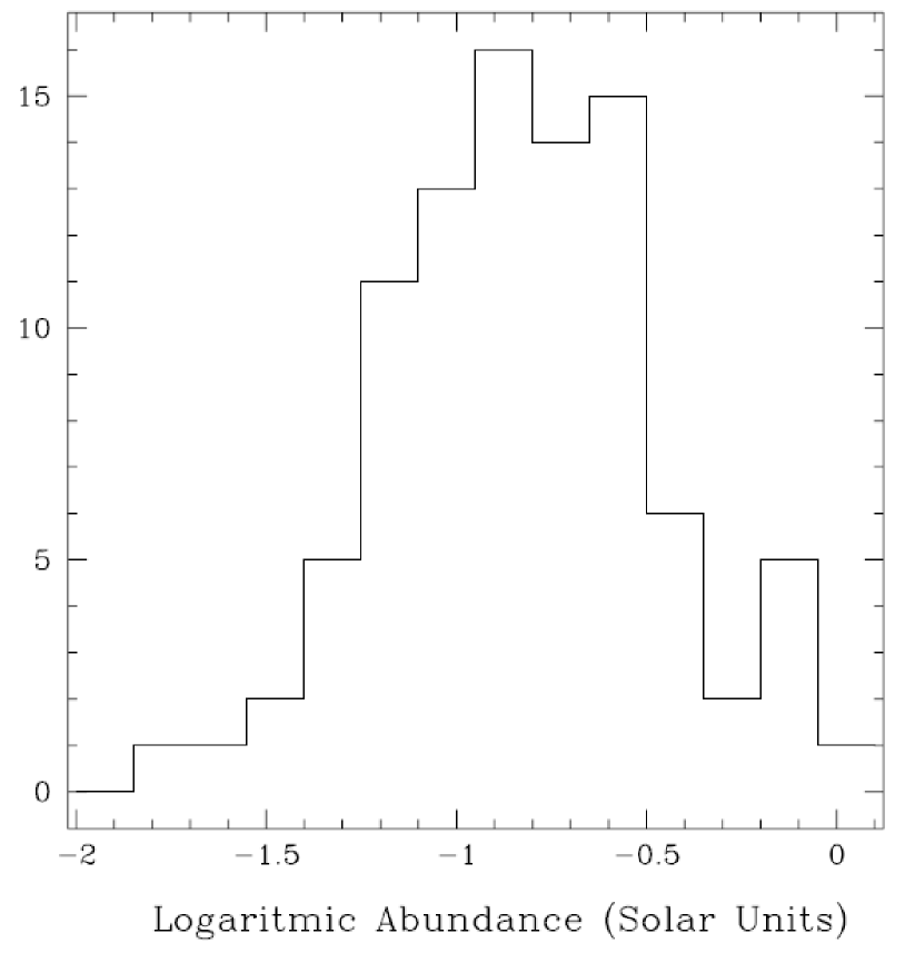
Figure 3.1: The metallicity distribution of H ii galaxies from Terlevich et al. (1991), as measured form the oxygen abundances. Taken from Kunth & Östlin (2000).

The metallicity of H ii galaxies was first analysed by Searle & Sargent (1972); they showed that oxygen and neon abundances for I Zw18 and II Zw40 were sub-solar, whereas He abundances where about solar supporting He as a primordial element. Subsequently, many works have addressed this issue (e.g. Alloin, Bergeron & Pelat, 1978; Lequeux et al., 1979; French, 1980; Kinman & Davidson, 1981; Kunth & Sargent, 1983; Terlevich et al., 1991; Pagel et al., 1992).

H ii galaxies are metal poor systems, the abundance of metals in these systems ranges between $1/2\ \mathrm{Z_{\odot}}$ and $1/50\ \mathrm{Z_{\odot}}$. Figure 3.1 shows the oxygen abundances distribution for a sample of Terlevich et al. (1991) H ii galaxies.

The oxygen abundance is normally considered as representative of the metallicity of H ii galaxies, as oxygen is the most abundant of the metals that constitute them. However, the abundances of other elements can be obtained too. Particularly interesting is the fact that since, in general, H ii galaxies are chemically unevolved systems, the analysis of helium abundances in these systems is a good method for determining primordial helium abundances (e.g. Pagel et al., 1992).

3.2 The $L(\mathrm{H}\beta)-\sigma$ Relation for H ii Galaxies

Melnick (1978) found a correlation between the average turbulent velocity of H ii regions in late spirals and irregular galaxies and the parent galaxy absolute magnitude, however at that moment the physics behind the correlation was not clear.

Terlevich & Melnick (1981) analysed the relation between $\mathrm{H}\beta$ luminosity, linewidth, metallicity and size for giant H ii regions and H ii galaxies finding correlations of the form:

$$luminosity \propto(linewidth)^{4}$$

$$size \propto(linewidth)^{4},$$

which are of the kind encountered in pressure supported systems, then they conclude that H ii galaxies (and giant H ii regions) are self-gravitating systems in which the observed emission-line profile widths represent the velocity dispersion of discrete gas clouds in the gravitational potential. Furthermore, they found that the scatter in the $L-\sigma$ relation was correlated to metallicity.

Melnick et al. (1987) analysed the properties of GEHRs. They found that the turbulent motions of the gaseous component of those systems are supersonic. Furthermore, they obtain correlations of the form:

$$R_{c} \sim\sigma^{2.5\pm 0.5}$$

$$L(\mathrm{H}\beta) \sim\sigma^{5.0\pm 0.5};$$

and they confirm the correlation between the scatter in the relations and the metallicity (from oxygen abundance). They concluded that the encountered relations are an indication of the virialized nature of discrete gas fragments forming the structure of the giant H ii regions and being ionised by a central star cluster. However, they recognise the possibility that stellar winds could have some, then unknown, effect on the velocity dispersion of the nebular gas.

Melnick, Terlevich & Moles (1988) studied the $L(\mathrm{H}\beta)-\sigma$ relation for H ii galaxies in a sample of objects that later would be part of the Spectrophotometric Catalogue of H ii Galaxies (Terlevich et al., 1991); they found a relation of the form:

$$\log L(\mathrm{H}\beta)=(4.70\pm 0.30)\log\sigma+(33.61\pm 0.50) \delta\log L(\mathrm{H}\beta)=0.29.$$ (3.1)

After a Principal Component Analysis (PCA) for the data, in which the oxygen abundance was used as parameter, they found that the metallicity, $(\mathrm{O/H})$, is effectively an important component of the scatter in the previous relation. Consequently, they proposed as a distance indicator:

$$M_{z}=\frac{\sigma^{5}}{(\mathrm{O/H})},$$ (3.2)

from which they obtain a new relation:

$$\log L(\mathrm{H}\beta)=(1.0\pm 0.04)\log M_{z}+(41.32\pm 0.08) \delta\log L(\mathrm{H}\beta)=0.271$$ (3.3)

We must note that this last relation uses the distance scale of Aaronson et al. (1986) ($H_{0}\sim 90\ \mathrm{Km\ s^{-1}\ Mpc^{-1}}$).

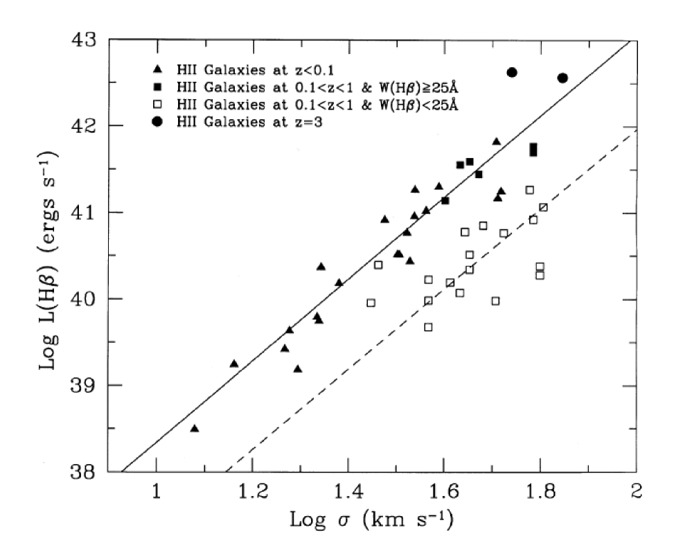
Figure 3.2: The $L(\mathrm{H}\beta)-\sigma$ relation for H ii galaxies at intermediate redshifts. The solid line shows the maximum-likelihood fit to the young H ii galaxies in the local Universe. The dashed line shows the predicted $L(\mathrm{H}\beta)-\sigma$ relation for an evolved population of H ii galaxies. The cosmology is $H_{0}=65\ \mathrm{km\ s^{-1}\ Mpc^{-1}}$. Taken from Melnick, Terlevich & Terlevich (2000).

Melnick, Terlevich & Terlevich (2000) selected a sample of intermediate redshift ($z<1$) H ii galaxies from the literature, using as selection criterion the emission lines strength. The objects with strongest emission lines (i.e. largest equivalent widths) were selected in order to avoid the evolved ones (Copetti, Pastoriza & Dottori, 1986), which can introduce a systematic error in the $L(\mathrm{H}\beta)-\sigma$ relation due to the effect of the underlying old population over the line widths. Using this sample, they found the $L(\mathrm{H}\beta)-\sigma$ relation shown in Figure 3.2; we can see clearly the effect of the stellar population evolution over the relation. In this work the distance indicator was re-calibrated with the then available distances for the sample. They found

$$\log L(\mathrm{H}\beta)=\log M_{z}+29.5,$$ (3.4)

from which they derived the distance modulus as

$$\mu=2.5\log\frac{\sigma^{5}}{F(\mathrm{H}\beta)}-2.5\log(\mathrm{O/H})-A_{\mathrm{H}\beta}-26.44,$$ (3.5)

where $F(\mathrm{H}\beta)$ is the observed $\mathrm{H}\beta$ flux and $A_{\mathrm{H}\beta}$ is the total extinction.

The differential Hubble diagram for H ii galaxies derived by Melnick, Terlevich & Terlevich (2000) is shown in Figure 3.3. From the figure it is clear that the data present large scatter with respect to the models differences. For the local sample ($z<0.1$), they derived an rms dispersion in distance modulus of $\sigma(\Delta\mu)=0.52\ \mathrm{mag}$. Melnick, Terlevich & Moles (1988) claim that typical errors are about 10% in flux and 5% in $\sigma$, adding 10% in extinction and 20% in abundances, while Melnick, Terlevich & Terlevich (2000) expect a scatter of about $0.35\ \mathrm{mag}$ in $\mu$ from observational errors. Hence, improvement in measurements is required in order to obtain better constraints.

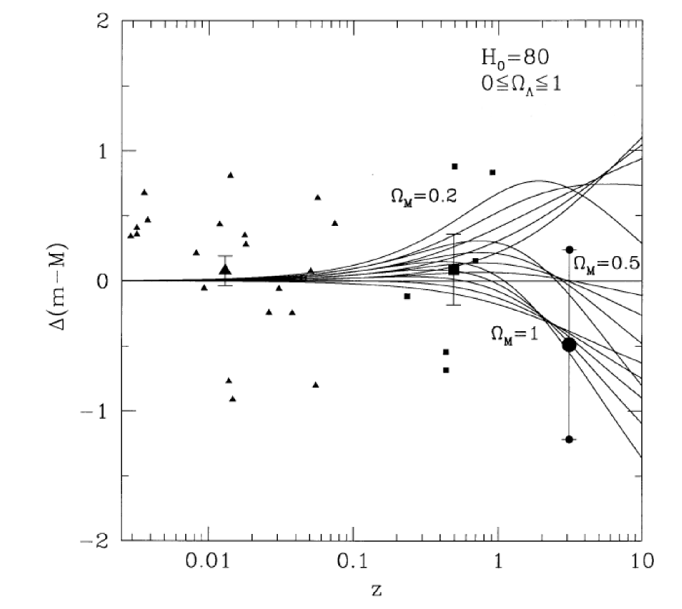
Figure 3.3: The differential Hubble diagram for H ii galaxies with a wide range of redshifts. Three families of curves for distinct values of $\Omega_{m}$ are shown, for every one $\Omega_{\Lambda}=(0,0.25,0.5,0.75,1.0)$. The large symbols represent the average redshift and distance modulus for each subsample. The error bars show the mean error in distance modulus assuming that each point is an independent measurement and ignoring observational errors. $H_{0}=80\ \mathrm{km\ s^{-1}\ Mpc^{-1}}$ was used to normalize the data points. The model lines are independent of $H_{0}$. From Melnick, Terlevich & Terlevich (2000).

Siegel et al. (2005) have constrained the value of $\Omega_{m}$ using a sample of 15 high-$z$ H ii galaxies ($2.17<z<3.39$) obtaining a best fit of $\Omega_{m}=0.21_{-0.12}^{+0.30}$ for a $\Lambda$-dominated universe, which is consistent with other recent determinations. Their sample has been selected using the criterion of emission line strength, as was selected in the Melnick, Terlevich & Terlevich (2000) sample. For the $\mu$ determination they have used (3.5) with a modification in the zero point (they used $26.18$ in place of $26.44$) due to the fact that they have taken $H_{0}=71\ \mathrm{km\ s^{-1}\ Mpc^{-1}}$.

3.2.1 The physics of the $L(\mathrm{H}\beta)-\sigma$ relation

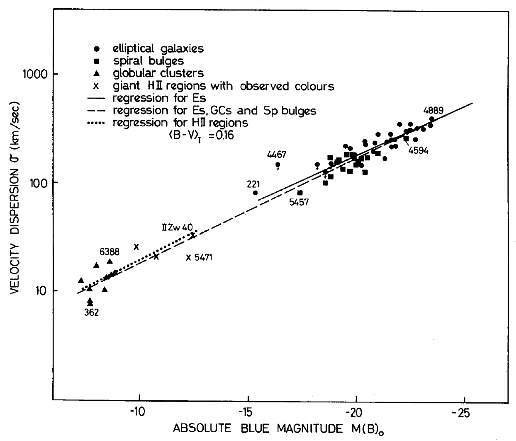
Figure 3.4: $M(B)_{0}-\sigma$ correlation for elliptical galaxies, bulges of spiral galaxies, globular clusters and GEHR. The dashed line is a linear fit for all the data. The solid line is a fit for elliptical galaxies. The dotted line is a fit to the GEHR. Taken from Terlevich & Melnick (1981).

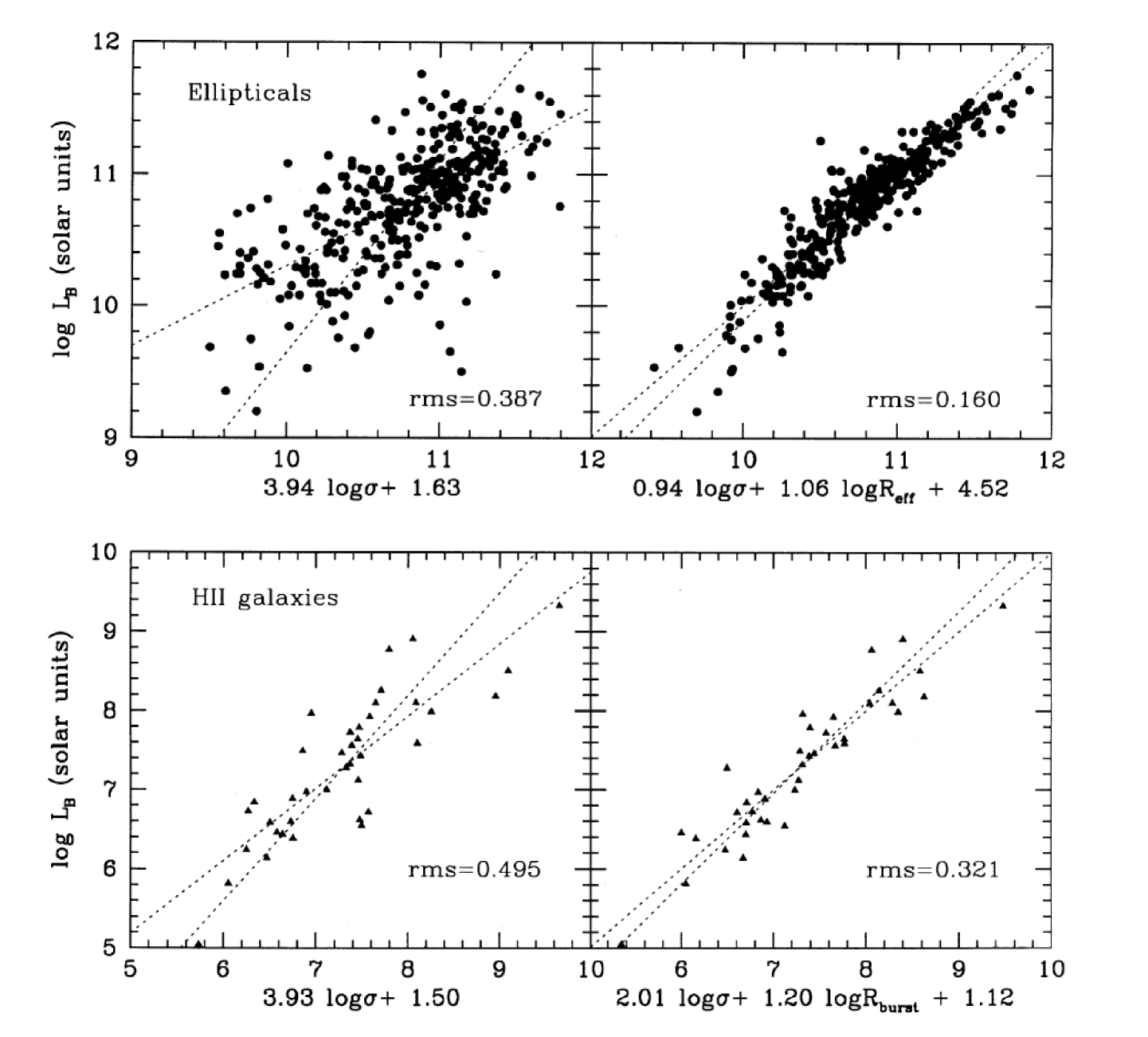
Figure 3.5: The fundamental plane of H ii galaxies and normal elliptical galaxies from Telles (1995). The radii and magnitudes of H ii galaxies are measured from continuum images. The velocity dispersions are the widths of the emission lines.

Melnick et al. (1987) found that H ii galaxies present supersonic motions in their gaseous component. In order to explain the motions of the H ii galaxies gaseous component, Terlevich & Melnick (1981) had proposed a model in which its nature is explained as being of gravitational origin. The basis for this argument is that correlations of the kind $L(\mathrm{H}\beta)\propto\sigma^{4}$ and $R\propto\sigma^{2}$ were observed in H ii galaxies. These correlations are expected for virialized systems and in fact are observed in elliptical galaxies, spiral bulges and globular clusters.

In order to compare GEHR with globular clusters, bulges of spirals and elliptic galaxies, and thus test the hypothesis of the gravitational origin for the $L(\mathrm{H}\beta)-\sigma$ relation, Terlevich & Melnick (1981) evolved the ionising stellar clusters following the single burst of star formation model by Larson & Tinsley (1978). The resulting $M(B)_{0}-\sigma$ relation is shown in Figure 3.4. From the figure it is clear that the $M(B)_{0}-\sigma$ relation for GEHR is consistent, within uncertainties, with the relations for the other spheroidal systems, strongly suggesting a mainly gravitational origin for the correlation.

Another factor that contributes to the origin of the supersonic turbulent motions in the gaseous component of H ii galaxies is the stellar winds generated by massive evolved stars. It has been shown that, unlike the case for evolved GEHRs where this effect dominates (Melnick, Tenorio-Tagle & Terlevich, 1999), for H ii galaxies it appears not to be dominant.

A strong support for the gravitational origin idea came from Telles (1995), where it was shown that these objects define a fundamental plane that is very similar to that defined by elliptical galaxies (see Figure 3.5). However, the scatter observed in the $L(\mathrm{H}\beta)-\sigma$ may be due to the presence of a second parameter, perhaps possible variations in the initial mass function (IMF), rotation or the duration of the burst of star formation that powers the emission lines (Melnick, Terlevich & Terlevich, 2000).

It has been shown that the scatter in the $L(\mathrm{H}\beta)-\sigma$ relation can be reduced if objects with $\sigma>65\ \mathrm{kms^{-1}}$ are rejected from the analysis (Melnick, Terlevich & Moles, 1988; Koo et al., 1995). This can be understood if one assumes that H ii galaxies are powered by clusters of stars, and thus the above condition is equivalent to say that the time required for the clusters to form must be smaller than the main sequence lifetime of the most massive stars (Melnick, Terlevich & Terlevich, 2000).

3.2.2 Age effects

Around $3\ \mathrm{Myr}$ to $6\ \mathrm{Myr}$ after a starburst, the emission line flux decays fast and continuously whereas the continuum flux is roughly constant. Thus, the equivalent widths ($W$) of emission lines are a good estimator of the starburst age (Copetti, Pastoriza & Dottori, 1986). In order to minimize systematic effects over the $L(\mathrm{H}\beta)-\sigma$ relation it is necessary to consider this effect by restricting the sample to objects with high $W(\mathrm{H}\beta)$ in order to select young starbursts and minimize the effects of a possible old underlying population over the equivalent width of the emission lines.

3.2.3 Extinction effects

Due to its effect over the flux of the $\mathrm{H}\beta$ line, the extinction or reddening is one important systematic for the $L(\mathrm{H}\beta)-\sigma$ relation. Two possible sources of extinction must be considered: dust in our Galaxy and dust in the H ii galaxies themselves. It has been shown that the extinction correction for H ii galaxies can be determined from Balmer decrements (Melnick et al., 1987; Melnick, Terlevich & Moles, 1988).

3.2.4 Metallicity effects

The metallicity has an important effect over the $L(\mathrm{H}\beta)-\sigma$ relation as was pointed out in the analysis of Terlevich & Melnick (1981) where it was shown that the residuals of this relation are correlated with metallicity. Furthermore, using PCA, Melnick et al. (1987) showed that one of the two principal components with the larger weight was mostly determined by the oxygen abundance.

3.3 H ii Galaxies as Cosmological Probes

This work’s main aim is to constrain the parameter space of the dark energy equation of state and therefore we will review briefly the theoretical analysis of the parameters involved.

From (2.20) we know that the Hubble function depends on the cosmological parameters following the relation:

$$H^{2}(z)=H_{0}^{2}\left[\Omega_{m}(1+z)^{3}+\Omega_{w}\exp\left(3\int_{0}^{z}{\frac{1+w(z^{\prime})}{1+z^{\prime}}dz^{\prime}}\right)\right],$$ (3.6)

where we are neglecting the minuscule contribution of the radiation to the total energy density and we are assuming a flat universe. From (2.33) we also know that:

$$\mu=5\log D_{L}+25,$$ (3.7)

where $D_{L}$, the luminosity distance, is given by (2.31) and is expressed in Mpc.

Using (3.6) we can define a nominal reference $\Lambda$-cosmology with $\Omega_{m}=0.27,\Omega_{\Lambda}=0.73$ and $w=-1$. And then we can compare different models to the reference one. For this purpose we define:

$$\Delta\mu=\mu_{\Lambda}-\mu_{model}\;,$$ (3.8)

where $\mu_{\Lambda}$ is the distance modulus given by the reference $\Lambda$-cosmology and $\mu_{model}$ is the one given by any another model.

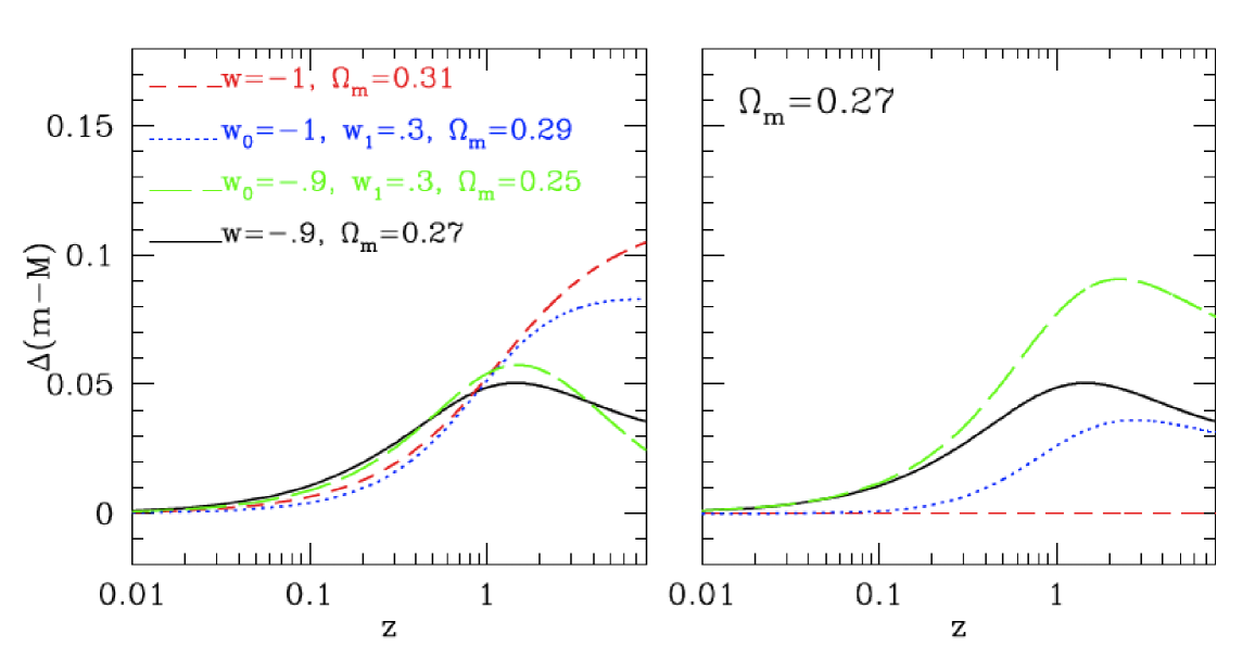
Figure 3.6: Left Panel: The expected distance modulus difference between the dark energy models shown and the reference $\Lambda$-model. Right Panel: The expected distance modulus differences once that the $\Omega_{m}-w(z)$ degeneracy is broken (imposing a unique $\Omega_{m}$ to all models). Taken from Plionis et al. (2009).

Figure 3.6 shows the difference between some cosmological models for which their parameters are indicated. It can be seen that the relative magnitude deviations between dark energy models is $\leq 0.1\ \mathrm{mag}$, which indicates the necessary high accuracy in the photometry of any object used as a tracer. Furthermore, it is clear that larger relative deviations of the distance moduli are present at $z\geq 1.5$, and therefore high-$z$ tracers are needed to effectively constrain the values of the equation of state parameters, in fact at redshifts higher than those currently probed by SNe Ia.

Another important factor, that we can see in Figure 3.6, is that there are strong degeneracies between different cosmological models at $z\leq 1$ (in some cases even at higher redshifts), this due to the known $\Omega_{m}-w(z)$ degeneracy. This fact shows the necessity of at least two independent cosmological probes in order to break the degeneracies. If we additionally consider that we have abundant evidence for $0.26\leq\Omega_{m}\leq 0.3$, we can expect that the degeneracies would be considerably reduced, as in fact is shown in the right hand panel of Figure 3.6, where we have fixed the value of $\Omega_{m}=0.27$.

Table 3.1: Cosmological parameters fits using the SNe Ia data within flat cosmologies. Note that for the case where $\mathbf{p}=(\Omega_{m},w)$ (last row), the errors shown are estimated after marginalizing with respect to the other fitted parameters. Taken from Plionis et al. (2010).

D07			Constitution
$w$	$\Omega_{m}$	$\chi^{2}_{min}/df$	$w$	$\Omega_{m}$	$\chi^{2}_{min}/df$
$\mathbf{-1}$ (fixed)	$0.280_{-0.015}^{+0.025}$	$187.03/180$	$\mathbf{-1}$ (fixed)	$0.286_{-0.018}^{+0.012}$	$439.78/365$
$-1.025_{-0.045}^{+0.060}$	$0.292\pm 0.018$	$187.02/179$	$-1.025\pm 0.030$	$0.298\pm 0.012$	$439.79/364$

As previously mentioned, the single available direct test for cosmic acceleration is based on the SNe Ia distance-redshift relation, and therefore it is useful to test how the constraints of the cosmological parameters change when the SNe Ia sample is increased. Plionis et al. (2010) analyse two SNe Ia data sets, the Davis et al. (2007) [hereafter D07] compilation of 192 SNe Ia and the Constitution compilation of 397 SNe Ia (Hicken et al., 2009), which are not independent since most of the D07 is included in the Constitution sample.

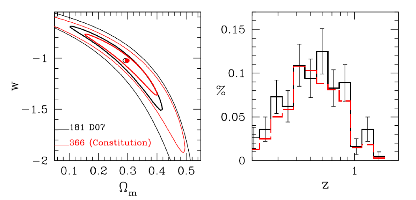
Figure 3.7: Left Panel: Cosmological parameters solution space using either of the two SNe Ia data sets (Constitution: red contours and D07: black contours). Contours corresponding to the $1$ and $3\sigma$ confidence levels are shown. Right Panel: Normalized redshift distribution of the two SNe Ia data sets. Taken from Plionis et al. (2010).

In order to perform the data analysis, a likelihood estimator (see Appendix C) was defined as:

$$\mathcal{L}^{SNIa}(\mathbf{p})\propto\exp[-\chi^{2}_{SNIa}(\mathbf{p})/2],$$ (3.9)

where $\mathbf{p}$ is a vector containing the cosmological parameters that we want to fit for, and

$$\chi^{2}_{SNIa}(\mathbf{p})=\sum_{i=1}^{N}{\left[\frac{\mu^{th}(z_{i},\mathbf{p})-\mu^{obs}(z_{i})}{\sigma_{i}}\right]^{2}},$$ (3.10)

where $\mu^{th}$ is given by (3.7) and (3.6), $z_{i}$ is the observed redshift, $\mu^{obs}$ is the observed distance modulus and $\sigma_{i}$ is the observed distance modulus uncertainty. A flat universe was assumed for the analysis so $\mathbf{p}\equiv(\Omega_{m},w_{0},w_{1})$. Finally, since only SNe Ia with $z>0.02$ were used in order to avoid redshift uncertainties due to peculiar motions, the final samples were of 181 (D07) and 366 (Constitution) SNe Ia.

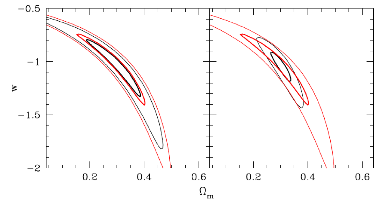
Figure 3.8: Left Panel: Comparison of the Constitution data set derived constraints (red contours) with those derived by reducing to half their uncertainties (black contours). Right Panel: Comparison of constrains from Constitution (red contours) with those derived by adding a sample of $82$ high-$z$ tracers ($2.7\lesssim z\lesssim 3.5$) with distance modulus mean uncertainty of $\sigma_{\mu}\simeq 0.38$ (black contours). Taken from Plionis et al. (2010).

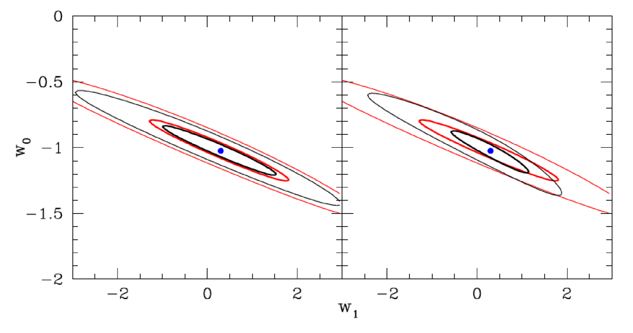
Figure 3.9: As in Figure 3.8, but allowing for an evolving Dark Energy equation of state and after marginalizing with respect to $\Omega_{m}$. The input cosmological model has $(w_{0},w_{1})=(-1.025,0.3)$ and is represented by the red contours. Taken from Plionis et al. (2010).

Table 3.1 presents solutions using the previous mentioned data sets. We can see that the cosmological parameters derived are consistent between both data sets.

Figure 3.7 shows the cosmological parameters solution space for the two above mentioned data sets. We can see that although the Constitution data set has twice as many data points as D07, the constraints obtained form the former are similar to those obtained from the latter. This fact indicates that, for Hubble function tracers, increasing the number of data points covering the same redshift range and with the current uncertainty level for SNe Ia, does not provide significantly better constraints for cosmological parameters.

From the previous discussion it becomes clear that we have two possible options to obtain more stringent constraints of cosmological parameters:

• Trace the same redshift range ($z\lesssim 1.5$), that has been traced until now using SNe Ia, but reducing significantly the distance modulus uncertainties or

• Trace at higher redshifts, where the different theoretical models show the largest deviations, maintaining or if possible reducing the distance modulus uncertainties now obtained for high-$z$ SNe Ia ($\langle\sigma_{\mu}\rangle\simeq 0.4$).

Plionis et al. (2010) analysed both alternatives by means of a Monte-Carlo procedure, and as it is shown in Figure 3.8, when the Constitution data uncertainties are reduced by half, the reduction in the range of the solution space is quite small; however, when a high-$z$ 82 mock-object subsample, with distance modulus uncertainties comparable to those of actual high-$z$ SNe Ia data, is added to the Constitution data set, a significantly reduced solution space is found. It is important to note that the redshift distribution ($2.68\lesssim z\lesssim 3.55$), for the added mock subsample, is in the range where the largest deviations between different cosmological models are expected (see Figure 3.6). The same behavior was found when an evolving dark energy equation of state model was implemented (see Figure 3.9).

From the previous discussion it is clear that in order to obtain more stringent constraints to the cosmological parameters, using the Hubble relation, a better strategy is to use standard candles which trace a redshift range where larger differences between the cosmological models are expected ($2\lesssim z\lesssim 4$).

Near infrared surveys (Pettini et al., 2001; Erb et al., 2003) have shown that H ii galaxies can be observed at much larger redshifts than SNe Ia and since they can be used as standard candles, due to their $L(\mathrm{H}\beta)-\sigma$ relation, they are excellent candidates for high-$z$ tracers to be used to constrain the cosmological parameters.

3.4 Summary

H ii galaxies are young massive bursts of star formation whose spectra is dominated by strong emission lines. These objects have been proposed as an useful standard candle, because their velocity dispersion is correlated with the luminosity of their Balmer emission lines.

The origin of the H ii galaxies $L(\mathrm{H}\beta)-\sigma$ relation has been studied in many works, with the general conclusion that virialization of the cluster gas appears to be the main cause, although other factors, as metallicity and age, also contribute to the relation.

Since H ii galaxies can be observed to $z\sim 3$, they constitute a promising new cosmic tracer which may allow to obtain better constraints to cosmological parameters than currently obtained with lower redshift tracers.

In the next chapter we will explore in depth the $L(\mathrm{H}\beta)-\sigma$ relation for H ii galaxies and the systematics affecting it.

Chapter 4 The $L-\sigma$ Relation for Massive Bursts of Star Formation

It is not knowledge, but the act of learning, not possession but the act of getting there, which grants the greatest enjoyment.

— C. F. Gauss, Letter to F. Bolyai (1808)

To build a robust model of the Universe it is necessary not only to set the strongest possible constraints on the cosmological parameters, applying joint analyses of a variety of distinct methodologies, but also to confirm the results through extensive consistency checks, using independent measurements and different methods, in order to identify and remove possible systematic errors, related to either the methods themselves or the tracers used.

It is accepted that young massive star clusters, like those responsible for the ionisation in giant extragalactic H ii regions (GEHR) and H ii galaxies display a correlation between the luminosity and the width of their emission lines, the $L(\mathrm{H}\beta)-\sigma$ relation (Terlevich & Melnick, 1981). The scatter in the relation is small enough that it can be used to determine cosmic distances independently of redshift (Melnick et al., 1987; Melnick, Terlevich & Moles, 1988; Siegel et al., 2005; Bordalo & Telles, 2011; Plionis et al., 2011; Chávez et al., 2012, 2014).

Recently Bordalo & Telles (2011) have explored the $L(\mathrm{H}\alpha)-\sigma$ correlation and its systematic errors using a nearby sample selected from the Terlevich et al. (1991) spectrophotometric catalogue of H ii galaxies ($0\lesssim z\lesssim 0.08$). They conclude that considering only the objects with clearly gaussian profiles in their emission lines, they obtain something close to an $L(\mathrm{H}\alpha)\propto\sigma^{4}$ relation with an rms scatter of $\delta\log L(\mathrm{H}\alpha)\sim 0.30$. It is important to emphasise that the observed properties of H ii galaxies, in particular the derived $L(\mathrm{H}\beta)-\sigma$  relation, are mostly those of the young burst and not those of the parent galaxy. This is particularly true if one selects those systems with the largest equivalent width (EW) in their emission lines, i.e. EW(H$\beta)>50$Å . The selection of those H ii galaxies having the strongest emission lines minimises the evolutionary effects in their luminosity (Copetti, Pastoriza, & Dottori, 1986), which would introduce a systematic shift in the $L(\mathrm{H}\beta)-\sigma$ relation due to the rapid drop of the ionising flux after 5 Myr of evolution. This selection minimises also any possible contamination in the observable due to the stellar populations of the parent galaxy.

A feature of the H ii galaxies optical spectrum, their strong and narrow emission lines, makes them readily observable with present instrumentation out to $z\sim 3.5$. Regarding such distant systems, Koo et al. (1995) and also Guzmán et al. (1996) have shown that a large fraction of the numerous compact star forming galaxies found at intermediate redshifts have kinematical properties similar to those of luminous local H ii galaxies. They exhibit fairly narrow emission line widths ($\sigma$ from 30 to 150 km/s) rather than the 200 km/s typical for galaxies of similar luminosities. In particular galaxies with $\sigma<$ 65 km/s seem to follow the same relations in $\sigma$, M_B and $L(\mathrm{H}\beta)$ as the local ones.

From spectroscopy of Balmer emission lines in a few Lyman break galaxies at $z\sim$ 3 Pettini et al. (1998) suggested that these systems adhere to the same relations but that the conclusions had to be confirmed for a larger sample. These results opened the important possibility of applying the distance estimator and mapping the Hubble flow up to extremely high redshifts and simultaneously to study the behaviour of starbursts of similar luminosities over a very large redshift range.

Using a sample of intermediate and high redshift H ii galaxies Melnick, Terlevich, & Terlevich (2000) investigated the use of the $L(\mathrm{H}\beta)-\sigma$ correlation as a high-$z$ distance indicator. They found a good correlation between the luminosity and velocity dispersion confirming that the $L(\mathrm{H}\beta)-\sigma$  correlation for local H ii galaxies is valid up to $z\sim$3. Indeed, our group (Plionis et al., 2011) showed that the H ii galaxies $L(\mathrm{H}\beta)-\sigma$ relation constitutes a viable alternative cosmic probe to SNe Ia. We also presented a general strategy to use H ii galaxies to trace the high-$z$ Hubble expansion in order to put stringent constraints on the dark energy equation of state and test its possible evolution with redshift. A first attempt by Siegel et al. (2005), using a sample of 15 high-$z$ H ii galaxies ($2.1<z<3.4$), selected as in Melnick, Terlevich & Terlevich (2000), with the original $L(\mathrm{H}\beta)-\sigma$ calibration of Melnick, Terlevich & Moles (1988), found a mass content of the universe of $\Omega_{m}=0.21_{-0.12}^{+0.30}$ for a flat $\Lambda$-dominated universe. Our recent reanalysis of the Siegel et al. (2005) sample (Plionis et al., 2011), using a revised zero-point of the original $L(H\beta)-\sigma$ relation, provided a similar value of $\Omega_{m}=0.22^{+0.06}_{-0.04}$ but with substantially smaller errors (see also Jarosik et al., 2011).

Recapitulating, we reassess the H ii galaxies $L(\mathrm{H}\beta)-\sigma$ relation using new data obtained with modern instrumentation with the aim of reducing the impact of observational random and systematic errors onto the H ii galaxies Hubble diagram. To achieve this goal, we selected from the SDSS catalogue a sample of 128 local ($z<0.2$), compact H ii galaxies with the highest equivalent width of their Balmer emission lines. We obtained high S/N high-dispersion echelle spectroscopic data with the VLT and Subaru telescopes to accurately measure the ionized gas velocity dispersion. We also obtained integrated H$\beta$ fluxes using low dispersion wide aperture spectrophotometry from the 2.1m telescopes at Cananea and San Pedro Mártir in Mexico, complemented with data from the SDSS spectroscopic survey.

This chapter follows closely our paper Chávez et al. (2014), its layout is as follows: we describe the sample selection procedure in §4.1, observations and data reduction in §4.2; an analysis in depth of the data error budget (observational and systematic) and the method for analysing the data are discussed in §4.3. The effect that different intrinsic physical parameters of the star-forming regions could have on the $L(\mathrm{H}\beta)-\sigma$  relation is studied in §4.4. The results for the $L(\mathrm{H}\beta)-\sigma$ relation is presented in §4.5, together with possible second parameters and systematic effects. Summary and conclusions are given in §4.7.

4.1 Sample Selection

We observed 128 H ii galaxies selected from the SDSS DR7 spectroscopic catalogue (Abazajian et al., 2009) for having the strongest emission lines relative to the continuum (i.e. largest equivalent widths) and in the redshift range $0.01<z<0.2$. The lower redshift limit was selected to avoid nearby objects that are more affected by local peculiar motions relative to the Hubble flow and the upper limit was set to minimize the cosmological non-linearity effects. Figure 4.1 shows the redshift distribution for the sample. The median of the distribution is also shown as a dashed line at $z\sim 0.045$, the corresponding recession velocity is $\sim 13500\ \mathrm{km\ s^{-1}}$.

Only those H ii galaxies with the largest equivalent width in their $\mathrm{H}\beta$ emission lines, $EW(\mathrm{H}\beta)>50\ \mathrm{\AA}$ were included in the sample. This relatively high lower limit in the observed equivalent width of the recombination hydrogen lines is of fundamental importance to guarantee that the sample is composed by systems in which a single very young starburst dominates the total luminosity. This selection criterion also minimizes the posible contamination due to an underlying older population or older clusters inside the spectrograph aperture (cf. Melnick, Terlevich & Terlevich, 2000; Dottori, 1981; Dottori & Bica, 1981). Figure 4.2 shows the $EW(\mathrm{H}\beta)$ distribution for the sample; the dashed line marks the median of the distribution, its value is $EW(\mathrm{H}\beta)\sim 87\ \mathrm{\AA}$.

Starbusrt99 (Leitherer et al., 1999, SB99) models indicate that an instantaneous burst with $EW(\mathrm{H}\beta)>50\ \mathrm{\AA}$ and Salpeter IMF has to be younger than about 5 Myr (see Figure 4.3). This is a strong upper limit because in the case that part of the continuum is produced by an underlying older stellar population, the derived cluster age will be even smaller.

Figure 4.1: Redshift distribution of the sample. The dashed line marks the median.

Figure 4.2: $\mathrm{H}\beta$ equivalent width distribution for the sample. The dashed line marks the median.

Figure 4.3: The evolution of the $\mathrm{H}\beta$ equivalent width for an instantaneous burst with metallicity Z$=0.004$ and a Salpeter IMF with upper limit of 100 M_⊙ (Leitherer et al., 1999). The horizontal line marks the $\mathrm{H}\beta$ equivalent width of 50 Å, while the vertical line indicates the corresponding age of $\sim$ 5 Myrs.

The sample is also flux limited as it was selected from SDSS for having an $\mathrm{H}\beta$ line core $\mathrm{h_{c}}(\mathrm{H}\beta)>100\times 10^{-17}\ \mathrm{erg\ s^{-1}cm^{-2}\AA^{-1}}$. To discriminate against high velocity dispersion objects and also to avoid those that are dominated by rotation, we have selected only those objects with $0.7<\sigma(\mathrm{H}\beta)<2.0\ \mathrm{\AA}$. From the values of the line core and $\sigma$ of the $\mathrm{H}\beta$ line we can calculate that the flux limit in the $\mathrm{H}\beta$ line is $F_{lim}(\mathrm{H}\beta)\sim 5\times 10^{-15}\ \mathrm{erg\ s^{-1}\ cm^{-2}}$ which corresponds to an emission-free continuum magnitude of $m_{B,lim}\simeq 19.2$ [cf. Terlevich & Melnick (1981) for the conversion].

To guarantee the best integrated spectrophotometry, only objects with Petrosian diameter less than 6^′′ were selected. In addition a visual inspection of the SDSS images was performed to avoid systems composed of multiple knots or extended haloes. Colour images from SDSS for a subset of objects in the sample are shown in Figure 4.4. The range in colour is related to the redshifts span of the objects and is due mainly to the dominant [OIII]$\lambda\lambda$4959,5007 doublet moving from the g to the r SDSS filters and to the RGB colour definition. The compactness of the sources can be appreciated in the figure.

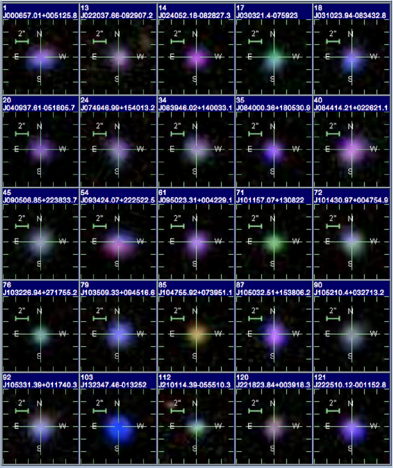
Figure 4.4: A selection of colour images of H ii galaxies from our sample. The SDSS name and our index number are indicated in the stamps. The changes in colour are related to the redshift of the object

4.2 Observations and Data Reduction

The data required for determining the $L(\mathrm{H}\beta)-\sigma$ relation are of two kinds:

1. Wide slit low resolution spectrophotometry to obtain accurate integrated emission line fluxes.

2. High resolution spectroscopy to measure the velocity dispersion from the $\rm{H}\beta$ and [OIII] line profiles. Typical values of the FWHM range from 30 to about 200$\ \rm{km\ s^{-1}}$.

A journal of observations is given in Table 4.1 where column (1) gives the observing date, column (2) the telescope, column (3) the instrument used, column (4) the detector and column (5) the projected slit width in arc seconds.

Table 4.1: Journal of observations.

(1)	(2)	(3)	(4)	(5)
Dates	Telescope	Instrument	Detector	Slit-width
5 & 16 Nov 2008	NOAJ-Subaru	HDS	EEV (2 $\times$ 2K $\times$ 4K)	4′′
16 & 17 Apr 2009	ESO-VLT	UVES-Red	EEV (2 $\times$ 2K $\times$ 4K)	2′′
15 - 17 Mar 2010	OAN - 2.12m	B&C	SITe3 (1K $\times$ 1K)	10′′
10 - 13 Apr 2010	OAGH - 2.12m	B&C	VersArray (1300 $\times$ 660)	8.14′′
8 -10 Oct 2010	OAN - 2.12m	B&C	Thompson 2K	13.03′′
7 - 11 Dic 2010	OAGH - 2.12m	B&C	VersArray (1300 $\times$ 660)	8.14′′
4 - 6 Mar 2011	OAN - 2.12m	B&C	Thompson 2K	13.03′′
1 - 4 Apr 2011	OAGH - 2.12m	B&C	VersArray (1300 $\times$ 660)	8.14′′

4.2.1 Low resolution spectroscopy

The low resolution spectroscopy for the line fluxes was performed with two identical Boller & Chivens Cassegrain spectrographs (B&C) in long slit mode at similar 2 meter class telescopes, one of them at the Observatorio Astronómico Nacional (OAN) in San Pedro Mártir (Baja California) and the other one at the Observatorio Astrofísico Guillermo Haro (OAGH) in Cananea (Sonora) both in México.

The observations at OAN were performed using a $600\ \mathrm{gr\ mm^{-1}}$ grating with a blaze angle of $8^{\circ}38^{\prime}$. The grating was centred at $\lambda\sim 5850\mathrm{\AA}$ and the slit width was 10^′′. The resolution obtained with this configuration is $R\sim 350$ ($\sim$ 2.07 Å/ pix) and the spectral coverage is $\sim 2100\ \mathrm{\AA}$. The data from OAGH was obtained using a $150\ \mathrm{gr\ mm^{-1}}$ grating with a blaze angle of $3^{\circ}30^{\prime}$ centred at $\lambda\sim 5000\mathrm{\AA}$. With this configuration and a slit width of 8.14^′′, the spectral resolution is $R\sim 83$ ($\sim$ 7.88 Å/ pix).

At least four observations of three spectrophotometric standard stars were performed each night. Futhermore, to secure the photometric link between different nights at least one H ii galaxy was repeated every night during each run. All objects were observed at small zenith distance, but for optimal determination of the atmospheric extinction the first and the last standard stars of the night were also observed at high zenith distance.

The wide-slit spectra obtained at OAN and OAGH were reduced using standard IRAF tasks. The reduction procedure entailed the following steps: (1) bias, flat field and cosmetic corrections, (2) wavelength calibration, (3) background subtraction, (4) flux calibration and (5) 1d spectrum extraction. The spectrophotometric standard stars for each night were selected among $\mathrm{G191-B2B}$, Feige 66, Hz 44, $\mathrm{BD+33d2642}$, GD 50, Hiltner 600, HR 3454, Feige 34 and GD 108.

We complemented our own wide-slit spectrophotometric observations with the SDSS DR7 spectroscopic data when available. SLOAN spectra are obtained with 3^′′diameter fibers, covering a range from $3200-9200\ \mathrm{\AA}$ and a resolution $R$ of $1850-2200$. The comparison between our own and SDSS spectrophotometry is discussed later on in §4.3.1.

4.2.2 High resolution spectroscopy

High spectral resolution spectroscopy for the line widths was obtained using echelle spectrographs at 8 meter class telescopes. The telescopes and instruments used are the Ultraviolet and Visual Echelle Spectrograph (UVES) at the European Southern Observatory (ESO) Very Large Telescope (VLT) in Paranal, Chile, and the High Dispersion Spectrograph (HDS) at the National Astronomical Observatory of Japan (NAOJ) Subaru Telescope in Mauna Kea, Hawaii (see Table 4.1 for the journal of observations).

UVES is a two-arm cross-disperser echelle spectrograph located at the Nasmyth B focus of ESO-VLT Unit Telescope 2 (UT2; Kueyen) (Dekker et al., 2000). The spectral range goes from $3000\ \mathrm{\AA}$ to $11000\ \mathrm{\AA}$. The maximum spectral resolution is $80000$ and $110000$ in the blue and red arm respectively. We used the red arm ($31.6\ \mathrm{gr\ mm^{-1}}$ grating, $75.04^{\circ}$ blaze angle) with cross disperser 3 configuration ($600\ \mathrm{gr\ mm^{-1}}$ grating) centred at $5800\ \mathrm{\AA}$. The width of the slit was 2^′′, giving a spectral resolution of $\sim 22500$ (0.014 Å/pix).

HDS is a high resolution cross-disperser echelle spectrograph located at the optical Nasmyth platform of NAOJ-Subaru Telescope (Noguchi et al., 2002; Sato et al., 2002). The instrument covers from $3000\ \mathrm{\AA}$ to $10000\ \mathrm{\AA}$. The maximum spectral resolution is $160000$. The echelle grating used has $31.6\ \mathrm{gr\ mm^{-1}}$ with a blaze angle of $70.3^{\circ}$. We used the red cross-disperser ($250\ \mathrm{gr\ mm^{-1}}$ grating, $5^{\circ}$ blaze angle) centred at $\sim 5413\ \mathrm{\AA}$ and a slit width of 4^′′, that provided a spectral resolution of $\sim 9000$ (0.054 Å/ pix).

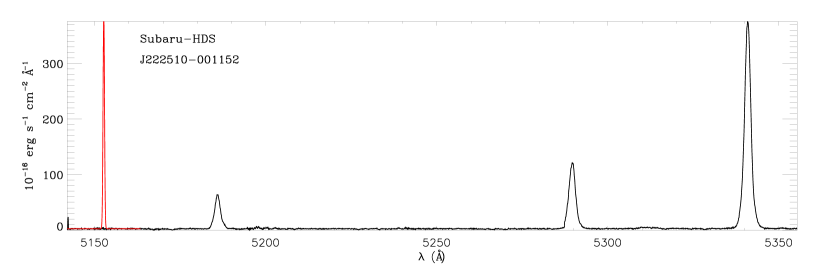
(a)

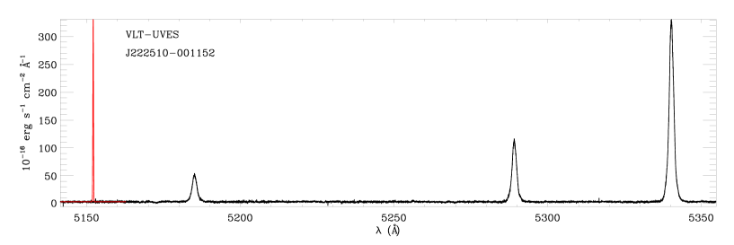
(b)

Figure 4.5: Examples of the high dispersion spectra obtained for the same object with Subaru HDS (top) and VLT UVES (bottom), showing the region covering $\mathrm{H}\beta\$ and the [OIII] lines at $\lambda\lambda$ 4959,5007 Å. The instrumental profile is shown in red at the left of each spectrum.

57 objects were observed with UVES and 76 with HDS. Five of them were observed with both instruments. During the UVES observing run 16 objects were observed more than once (three times for four objects and four times for another one) in order to estimate better the observational errors, and to link the different nights of the run. Two objects were observed twice with the HDS. The five galaxies observed at both telescopes also served as a link between the observing runs and to compare the performance of both telescopes/instruments and the quality of the nights.

Similarly, 59 sources were observed at OAGH and 59 at OAN, of which 15 were observed at both telescopes.

The UVES data reduction was carried out using the UVES pipeline V4.7.4 under the GASGANO V2.4.0 environment. The reduction entailed the following steps and tasks: (1) master bias generation (uves_cal_mbias), (2) spectral orders reference table generation (uves_cal_predict and uves_cal_orderpos), (3) master flat generation (uves_cal_mflat), (4) wavelength calibration (uves_cal_wavecal), (5) flux calibration (uves_cal_response) and (6) science objects reduction (uves_obs_scired).

The HDS data were reduced using IRAF packages and a script for overscan removal and detector linearity corrections provided by the NAOJ-Subaru telescope team. The reduction procedure entailed the following steps: (1) bias subtraction, (2) generation of spectral order trace template, (3) scattered light removal, (4) flat fielding, (5) 1d spectrum extraction and (6) wavelength calibration.

Typical examples of the high dispersion spectra are shown in Figure 4.5. The instrumental profile of each setup is also shown on the left.

4.3 Data Analysis.

We have already mentioned in §4.1 that we observed 128 H ii galaxies with EW(H$\beta$) $>50$ $\mathrm{\AA}$. From the observed sample we have removed 13 objects which presented problems in the data (low S/N) or showed evidence for a prominent underlying Balmer absorption. We also removed an extra object that presented highly asymmetric emission lines. After this we were left with 114 objects that comprise our ‘initial’ sample (S2).

It was shown by Melnick, Terlevich & Moles (1988) that imposing an upper limit to the velocity dispersion such as $\log\sigma($H$\beta)<1.8$ $\mathrm{km\ s^{-1}}$, minimizes the probability of including rotationally supported systems and/or objects with multiple young ionising clusters contributing to the total flux and affecting the line profiles. Therefore from S2 we selected all objects having $\log\sigma($H$\beta)<1.8$ $\mathrm{km\ s^{-1}}$ thus creating sample S3 – our ‘benchmark’ sample – composed of 107 objects.

A summary of the characteristics of the subsamples used in this chapter can be found in Table 4.2 and is further discussed in section 6. Column (1) of Table 4.2 gives the reference name of the sample, column (2) lists its descriptive name, column (3) gives the constraints that led to the creation of the subsample and column (4) gives the number of objects left in it.

Table 4.2: Samples Description.

(1)	(2)	(3)	(4)
Sample	Description	Constraints	N
S1	Observed	None	128
S2	Initial	S1 - all dubious data eliminated	114
S3	Benchmark	S2 - $\log\sigma$ (H$\beta)>1.8$	107
S4	10% cut	S3 - $\delta_{flux}(\mathrm{H}\beta)>10$, $\delta_{FWHM}(\mathrm{H}\beta)>10$	93
S5	Restricted	S3 - kinematical analysis	69

4.3.1 Emission line fluxes.

Given the importance of accurate measurements for our results, we will describe in detail our methods.

Total flux and equivalent width of the strongest emission lines were measured from our low dispersion wide-slit spectra. Three methods were used, we have obtained the total flux and equivalent width from single gaussian fits to the line profiles using both the IDL routine gaussfit and the IRAF task splot, and we also measured the fluxes integrated under the line, in order to have a measurement independent of the line shape.

Figure 4.6 shows a gaussian fit and the corresponding integrated flux measurement for an $\mathrm{H}\beta$ line from our low dispersion data. It is clear from the figure that in the cases when the line is asymmetric, the gaussian fit would not provide a good estimate of the actual flux. In the example shown the difference between the gaussian fit and the integration is $\sim 5.7\%$ in flux.

Table LABEL:tab:tab03 shows the results of our wide-slit low resolution spectroscopy measurements. The data listed have not been corrected for internal extinction. Column (1) is our index number, column (2) is the SDSS name, column (3) is the integrated $\mathrm{H}\beta$ flux measured by us from the SDSS published spectra, columns (4) and (5) are the $\mathrm{H}\beta$ line fluxes as measured from a gaussian fit to the emission line and integrating the line respectively, columns (6) and (7) are the $[\mathrm{O\ III}]\ \lambda\lambda 4959$ and $5007$ line fluxes measured from a gaussian fit, column (8) gives the EW of the $\mathrm{H}\beta$ line as measured from the SDSS spectra and column (9) is a flag that indicates the origin of the data and is described in the table caption.

Figure 4.7 shows the comparison between SDSS and our low resolution spectra. Clearly most of the objects show an excess flux in our data which could easily be explained as an aperture effect, as the $3\hbox{${}^{\prime\prime}$}$ diameter fiber of SDSS in many cases does not cover all the object whereas our spectra were taken with apertures of $8\hbox{${}^{\prime\prime}$}-13\hbox{${}^{\prime\prime}$}$ in width, hence covering the entire compact object in all cases.

Figure 4.6: An example of gaussian fit (dashed line) and integration under the line (shaded area) for an $\mathrm{H}\beta$ line from the low dispersion data. The parameters for both fits are shown in the inset.

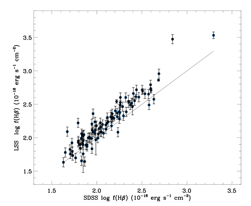
Figure 4.7: Fluxes measured from SDSS spectra compared with those measured from our low dispersion spectra (LS), the line shows the one-to-one correspondence.

Fluxes and equivalent widths of $[\mathrm{O\ II}]\ \lambda\lambda 3726,3729$, $[\mathrm{O\ III}]\ \lambda\lambda 4363,4959,5007$, $\mathrm{H}\gamma$, $\mathrm{H}\alpha$, $[\mathrm{N\ II}]\ \lambda\lambda 6548,6584$ and $[\mathrm{S\ II}]\ \lambda\lambda 6716,6731$ were also measured from the SDSS spectra when available. We have fitted single gaussians to the line profiles using both the IDL routine gaussfit and the IRAF task splot and, when necessary, we have de-blended lines by multiple gaussian fitting.

Table LABEL:tab:tab04 shows the results for the SDSS spectra line flux measurements as intensity relative to $\mathrm{H}\beta=100$. Columns are: (1) the index number, (2) the SDSS name, (3) and (4) the intensities of $[\mathrm{O\ II}]\ \lambda 3726$ and $\lambda 3729$, (5), (6) and (7) the intensities of $[\mathrm{O\ III}]\ \lambda 4363,\lambda 4959$ and $\lambda 5007$, (8) $\mathrm{H}\gamma$ intensity, (9) $\mathrm{H}\alpha$ intensity, (10) and (11) are the intensities of $[\mathrm{N\ II}]\ \lambda 6548$ and $\lambda 6584$ and (12) and (13) the intensities of the $[\mathrm{S\ II}]\ \lambda 6716$ and $\lambda 6731$ lines. The values given are as measured, not corrected for extinction. The 1$\sigma$ uncertainties for the fluxes are given in percentage.

In all cases, unless otherwise stated in the tables, the uncertainties and equivalent flux of the lines have been estimated from the expressions (Tresse et al., 1999):

$$\sigma_{F} = \sigma_{c}D\sqrt{2N_{pix}+EW/D},$$ (4.1)

$$\sigma_{EW} = \frac{EW}{F}\sigma_{c}D\sqrt{EW/D+2N_{pix}+(EW/D)^{2}/N_{pix}},$$ (4.2)

where $\sigma_{c}$ is the mean standard deviation per pixel of the continuum at each side of the line, $D$ is the spectral dispersion in $\mathrm{\AA\ pix^{-1}}$, $N_{pix}$ is the number of pixels covered by the line, $EW$ is the line equivalent width in $\mathrm{\AA}$, $F$ is the flux in units of $\mathrm{erg\ s^{-1}\ cm^{-2}}$. When more than one observation was available, the 1$\sigma$ uncertainty was given as the standard deviation of the individual determinations.

In order to characterise further the sample, a BPT diagram was drawn for the 99 objects of S3 that have a good measurement of $[\mathrm{O\ III}]\lambda$ 5007/ $\mathrm{H}\beta$  and $[\mathrm{N\ II}]\lambda$ 6584/$\mathrm{H}\alpha$  ratios. The diagram is shown in Figure 4.8 where it can be seen that clearly, all objects are located in a narrow strip just below the transition line (Kewley et al., 2001) indicating high excitation and suggesting low metal content and photoionisation by hot main sequence stars, consistent with the expectations for young H ii regions.

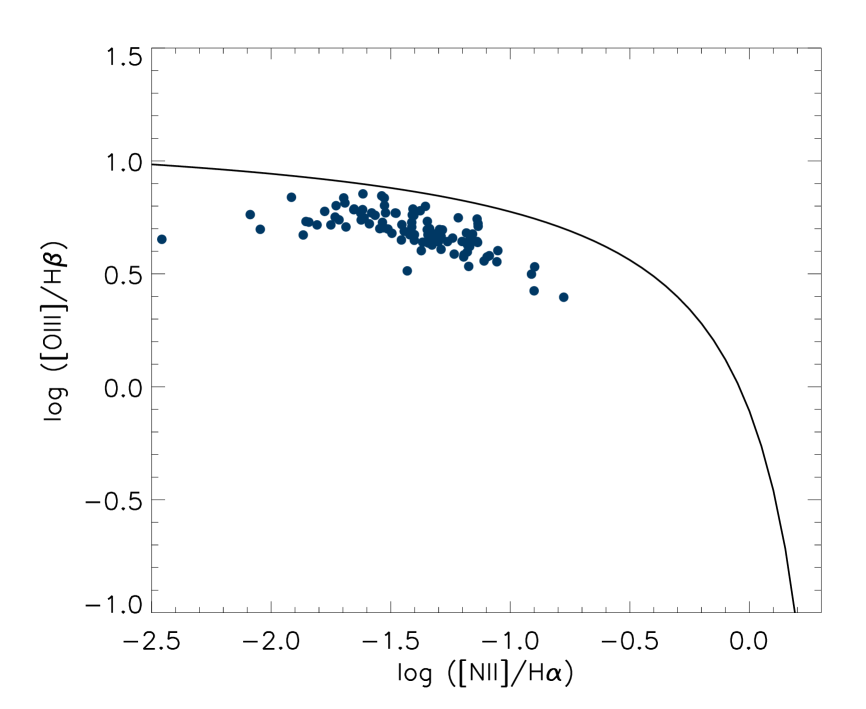
Figure 4.8: BPT diagram showing the high excitation level of a sample of H ii galaxies selected mainly as having high equivalent width in their Balmer emission lines. The solid line represents the upper limit for stellar photoionization, from Kewley et al. (2001).The plot shows 99 points from the S3 sample (see text).

4.3.2 Line profiles

From the two dimensional high dispersion spectra we have obtained the total flux, the position and the full width at half maximum (FWHM) of $\mathrm{H}\beta$ and $[\mathrm{O\ III}]\ \lambda\lambda 4959,5007$Å in each spatial increment i.e. along the slit.

These measurements were used to map the trends in intensity, position, centroid wavelength and FWHM of those emission lines. The intensity or brightness distribution across the object provides information about the sizes of the line and continuum emitting regions. The brightness distribution was used to determine the centroid and FWHM of the line emitting region. On the other hand the trend in the central wavelength of the spectral profile along the spatial direction was used to determine the amount of rotation present.

The trend in FWHM along the slit help us also to verify that there is no FWHM gradient across the object; any important change along the slit could affect the global measurements. In general it was found that the FWHM of the non-rotating systems is almost constant. Those systems with significant gradient or change, were removed from S3 leaving us with the sample used in Chávez et al. (2012) paper (S5) (see Chapter LABEL:CH:5). We call this procedure the ‘kinematic analysis’ of the emission line profiles.

The observed spatial FWHM of the emitting region was used to extract the one dimensional spectrum of each object. Three different fits were performed on the 1D spectra profiles (FWHM) of $\mathrm{H}\beta$ and the $[\mathrm{O\ III}]\ \lambda\lambda 4959,5007$Å lines: a single gaussian, two asymmetric gaussians and 3 gaussians (a core plus a blue and a red wing). These fits were performed using the IDL routines gaussfit, arm_asymgaussfit and arm_multgaussfit respectively. Figure 4.9 shows a typical fit to $\mathrm{H}\beta$; the best fitting to all the sample objects is presented in Appendix D.

Multiple fittings with no initial restrictions are not unique, so we computed using an automatized IDL code, a grid of fits each with slightly different initial conditions. From this set of solutions we chose those that had the minimum $\chi^{2}$. We begin with a blind grid of parameters from which the multiple gaussian fits are constructed, hence some of the resulting fits with small $\chi^{2}$ are not reasonable due to numerical divergence in the fitting procedure. We have eliminated unreasonable results by visual inspection.

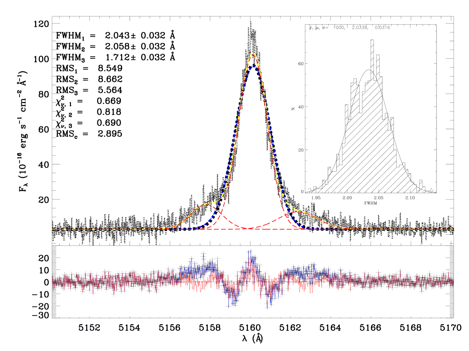
Figure 4.9: Typical multiple gaussian fit to an $\mathrm{H}\beta$ line. Upper panel: The single gaussian fit is shown with a dashed line (thick black). The asymmetric gaussian fit is indicated by the dash-dotted line (blue). In the three gaussians fit, every gaussian is indicated by long-dashed lines (red) and the total fit by a dash-double-dotted line (yellow). The parameters of the fits are shown in the top left corner. The inset shows the results from the Montecarlo simulation to estimate the errors in the parameters of the best fit. See further details in the text. Lower panel: The residuals from the fits follow the same colour code; the plusses are the residuals from the single gaussian fit whereas the continuous lines are the residuals from the asymmetric and three gaussian fits.

The 1$\sigma$ uncertainties of the FWHM were estimated using a Montecarlo analysis. A set of random realizations of every spectrum was generated using the data poissonian 1$\sigma$ 1-pixel uncertainty. Gaussian fitting for every synthetic spectrum in the set was performed afterwards, and we obtained a distribution of FWHM measurements from which the 1$\sigma$ uncertainty for the FWHM measured in the spectra follows. Average values obtained are 6.3% in H$\beta$ and 3.6% in [OIII].

Table LABEL:tab:tab02 lists the FWHM measurements for the high resolution observations prior to any correction such as instrumental or thermal broadening. Column (1) is the index number, column (2) is the SDSS name, columns (3) and (4) are the right ascension and declination in degrees, column (5) is the heliocentric redshift as taken from the SDSS DR7 spectroscopic data, columns (6) and (7) are the measured $\mathrm{H}\beta$ and $[\mathrm{O\ III}]\ \lambda 5007$ FWHM in Å.

4.3.3 Emission line widths

The observed velocity dispersions ($\sigma_{o}$) – and their 1$\sigma$ uncertainties – have been derived from the FWHM measurements of the $\mathrm{H}\beta$ and $[\mathrm{O\ III}]\lambda 5007$ lines on the high resolution spectra as:

$$\sigma_{o}\equiv\frac{FWHM}{2\sqrt{2\ ln(2)}}$$ (4.3)

Corrections for thermal ($\sigma_{th}$), instrumental ($\sigma_{i}$) and fine structure ($\sigma_{fs}$) broadening have been applied. The corrected value is given by the expression:

$$\sigma=\sqrt{\sigma_{o}^{2}-\sigma_{th}^{2}-\sigma_{i}^{2}-\sigma_{fs}^{2}}$$ (4.4)

We have adopted the value of $\sigma_{fs}(\mathrm{H}\beta)=2.4\ \mathrm{km\ s^{-1}}$ as published in García-Díaz et al. (2008). The 1$\sigma$ uncertainties for the velocity dispersion have been propagated from the $\sigma_{o}$ values.

The high resolution spectra were obtained with two different slit widths. The slit size was initially defined as to cover part of the Petrosian diameter of the objects. For UVES data, for which the slit width was 2^′′ and the slit was uniformly illuminated, $\sigma_{i}$ was directly estimated from sky lines, as usual. The Subaru observations have shown that the 4^′′ slit size used, combined with the excellent seeing during our observations has the unwanted consequence that the slit was not uniformly illuminated for the most compact H ii galaxies that tend to be also the most distant ones. Thus we have devised a simple procedure to calculate the instrumental broadening correction for the Subaru data. In this case, $\sigma_{i}$ was estimated from the target size; we positioned a rectangular area representing the slit over the corresponding SDSS r band image and measured from the image the FWHM of the object along the dispersion direction. In Figure 4.10 we plot $\sigma$ (after applying the broadening corrections as described above) for the five objects that have been observed with both instruments. It is clear that the results using both methods are consistent.

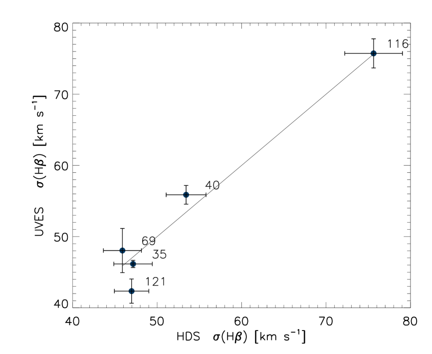
Figure 4.10: Comparison of $\sigma$ values after applying broadening corrections, as described in the text, for the 5 objects observed with both telescopes. The labels are the object indices as in the tables.

The thermal broadening was calculated assuming a Maxwellian velocity distribution of the hydrogen and oxygen ions, from the expression:

$$\sigma_{th}\equiv\sqrt{\frac{kT_{e}}{m}},$$ (4.5)

where $k$ is the Boltzmann constant, $m$ is the mass of the ion in question and $T_{e}$ is the electron temperature in degrees Kelvin as discussed in §4.4.3. For the H lines, an object with the sample median $\sigma_{0}$=37km/s, thermal broadening represents about 10%, $\sigma_{fs}$=0.3% and $\sigma_{inst-UVES}$=2% while $\sigma_{inst-HDS}$=9%. For the [OIII] lines, thermal broadening is less than 1%, typically 0.3%.

The obtained velocity dispersions for the $\mathrm{H}\beta$ and $[\mathrm{O\ III}]\lambda 5007$ lines are shown in Table LABEL:tab:tab05, in columns (7) and (8) respectively. Figure 4.11 shows the distribution of the $\mathrm{H}\beta$ velocity dispersions for the S3 sample (see Table 4.2).

Figure 4.11: Distribution of the $\mathrm{H}\beta$ velocity dispersion for the sample S3. The dashed line shows the median of the distribution.

4.3.4 Extinction and underlying absorption

Reddening correction was performed using the coefficients derived from the Balmer decrement, with $\rm{H}\alpha$, $\rm{H}\beta$ and $\rm{H}\gamma$ fluxes obtained from the SDSS DR7 spectra. However, contamination by the underlying stellar population produces Balmer stellar absorption lines under the Balmer nebular emission lines. This fact alters the observed emission line ratios in such a way that the Balmer decrement and the internal extinction are overestimated (see e.g. Olofsson, 1995).

To correct the extinction determinations for underlying absorption, we use the technique proposed by Rosa-González, Terlevich & Terlevich (2002). The first step is to determine the underlying Balmer absorption ($Q$) and the “true” visual extinction ($A_{V}$) from the observed one ($A_{V}^{*}$).

The ratio between a specific line intensity, $F(\lambda)$, and that of $\mathrm{H}\beta$, $F(\mathrm{H}\beta)$, is given by

$$\frac{F(\lambda)}{F(\mathrm{H}\beta)}=\frac{F_{0}(\lambda)}{F_{0}(\mathrm{H}\beta)}10^{-0.4A_{V}[k(\lambda)-k(\mathrm{H}\beta)]/R_{V}},$$ (4.6)

where $k(\lambda)=A(\lambda)/E(B-V)$ is given by the adopted extinction law, $R_{V}=A_{V}/E(B-V)$ is the optical total-to-selective extinction ratio and the subscript $0$ indicates unreddened intrinsic values.

We used as reference the theoretical ratios for Case B recombination $F_{0}(\mathrm{H}\alpha)/F_{0}(\mathrm{H}\beta)=2.86$ and $F_{0}(\mathrm{H}\gamma)/F_{0}(\mathrm{H}\beta)=0.47$(Osterbrock, 1989). In the absence of underlying absorption, the observed flux ratios can be expressed as a function of the theoretical ratios and the visual extinction:

$$\log\frac{F(\mathrm{H}\alpha)}{F(\mathrm{H}\beta)} =\log 2.86-0.4[k(\mathrm{H}\alpha)-k(\mathrm{H}\beta)]A_{V}/R_{V}\;,$$ (4.7)

$$\log\frac{F(\mathrm{H}\gamma)}{F(\mathrm{H}\beta)} =\log 0.47-0.4[k(\mathrm{H}\gamma)-k(\mathrm{H}\beta)]A_{V}/R_{V}\;.$$ (4.8)

Including the underlying absorption and assuming that the absorption and emission lines have the same widths (González-Delgado, Leitherer & Heckman, 1999), the observed ratio between $\mathrm{H}\alpha$ and $\mathrm{H}\beta$ is given by

$$\frac{F(\mathrm{H}\alpha)}{F(\mathrm{H}\beta)}=\frac{2.86\{1-PQ[W_{+}(\mathrm{H}\beta)/W_{+}(\mathrm{H}\alpha)]\}}{1-Q},$$ (4.9)

where $W_{+}(\mathrm{H}\alpha)$ and $W_{+}(\mathrm{H}\beta)$ are the equivalent widths in emission for the lines, $Q=W_{-}(\mathrm{H}\beta)/W_{+}(\mathrm{H}\beta)$ is the ratio between the equivalent widths of $\mathrm{H}\beta$ in absorption and in emission and $P=W_{-}(\mathrm{H}\alpha)/W_{-}(\mathrm{H}\beta)$ is the ratio between $\mathrm{H}\alpha$ and $\mathrm{H}\beta$ equivalent widths in absorption.

The value $P$ can be obtained theoretically from spectral evolution models. Olofsson (1995) has shown that for solar abundance and stellar mass in the range $0.1\ \mathrm{M_{\odot}}\leq M\leq 100\ \mathrm{M_{\odot}}$ using a Salpeter IMF, the value of $P$ is close to $1$ with a dispersion $\sim 0.3$ for ages between $1-15\ \mathrm{Myr}$. Since the variation of $P$ produces a change in the $F(\mathrm{H}\alpha)/F(\mathrm{H}\beta)$ ratio of less than 2 % that, given the low extinction in H ii galaxies, translates in a flux uncertainty well below 1 %, we have assumed $P=1$.

The ratio between $\mathrm{H}\gamma$ and $\mathrm{H}\beta$ is

$$\frac{F(\mathrm{H}\gamma)}{F(\mathrm{H}\beta)}=\frac{0.47-GQ}{1-Q},$$ (4.10)

where $G=W_{-}(\mathrm{H}\gamma)/W_{-}(\mathrm{H}\beta)$ is the ratio between the equivalent widths in absorption of $\mathrm{H}\gamma$ and $\mathrm{H}\beta$. Olofsson (1995, ; Tables 3a,b ) and González-Delgado, Leitherer & Heckman (1999, ; Table 1) suggest that the value of the parameter $G$ can also be taken as $1$.

When the theoretical values for the ratios $\log[F(\mathrm{H}\alpha)/F(\mathrm{H}\beta)]=0.46$ and $\log[F(\mathrm{H}\gamma)/F(\mathrm{H}\beta)]=-0.33$, are chosen as the origin, the observed ratios can define a vector for the observed visual extinction ($\mathbf{A_{V}^{*}}$). From equations (4.7) and (4.8) and a set of values for $A_{V}$, we define a vector for the “true” visual extinction, whereas from equations (4.9) and (4.10) and a set of values of $Q$, we define a vector for the underlying absorption $\mathbf{Q}$. Assuming that the vector relation $\mathbf{Q}+\mathbf{A_{V}}=\mathbf{A_{V}^{*}}$ is satisfied, by minimizing the distance between the position of the vector $\mathbf{A_{V}^{*}}$ and the sum $\mathbf{Q}+\mathbf{A_{V}}$ for every pair of parameters $(Q,A_{V})$, we obtain simultaneously the values for $Q$ and $A_{V}$ that correspond to the observed visual extinction.

The de-reddened fluxes were obtained from the expression

$$F_{o}(\lambda)=F_{obs}(\lambda)10^{0.4A_{V}k(\lambda)/R_{V}},$$ (4.11)

where the extinction law was taken from Calzetti et al. (2000). The 1$\sigma$ uncertainties were propagated by means of a Monte Carlo procedure.

Finally, the de-reddened fluxes were corrected for underlying absorption. For $\mathrm{H}\beta$ the correction is given by:

$$F(H\beta)=\frac{F_{o}(H\beta)}{1-Q}$$ (4.12)

The 1$\sigma$ uncertainties were propagated straightforwardly. The results are shown in Table LABEL:tab:tab05, columns (4), (5) and (6) where we give the values for $A_{V}$, $Q$ and $C_{\mathrm{H}\beta}$ respectively.

4.3.5 Redshifts and distances

Redshifts have been transformed from the heliocentric to the local group frame following Courteau & van den Bergh (1999) by the expression:

$$z_{lg}=z_{hel}-\frac{1}{c}(79\cos l\cos b-296\sin l\cos b+36\sin b),$$ (4.13)

where $z_{lg}$ is the redshift in the local group reference frame, $z_{hel}$ is the redshift in the heliocentric reference frame, $c$ is the speed of light and $l$ and $b$ are the galactic coordinates of the object.

We also corrected by bulk flow effects following the method proposed in Basilakos & Plionis (1998) and Basilakos & Plionis (2006). For this correction and since the objects in our sample have low redshifts, the distances have been calculated from the expression:

$$D_{L}\approx\frac{cz}{H_{0}},$$ (4.14)

where $z$ is the redshift and $D_{L}$ is the luminosity distance. For the Hubble constant we used a value of $H_{0}=74.3\pm 4.3\ \mathrm{km\ s^{-1}Mpc^{-1}}$ (Chávez et al., 2012). The 1$\sigma$ uncertainties for the distances were calculated using error propagation from the uncertainties in $z$ and $H_{0}$. Column (3) in Table LABEL:tab:tab05 (where we show all the parameters derived from the measurements) gives the corrected redshift.

4.3.6 Luminosities

The H$\beta$ luminosities were calculated from the expression:

$$L(\mathrm{H}\beta)=4\pi D_{L}^{2}F(\mathrm{H}\beta),$$ (4.15)

where $D_{L}$ is the previously calculated luminosity distance and $F(\mathrm{H}\beta)$ is the reddening and underlying absorption corrected H$\beta$ flux. The 1$\sigma$ uncertainties were obtained by error propagation.

Table LABEL:tab:tab05, column (9) shows the corrected $\mathrm{H}\beta$ luminosities obtained for the objects in the sample. Figure 4.12 shows the distribution of luminosities for the objects in S3. The median of the distribution is log(L($\mathrm{H}\beta$)) = 41.03 and the range is from 39.6 to 42.0.

Figure 4.12: Distribution of the $\mathrm{H}\beta$ emission line luminosities (and SFR as labelled on the top of the figure) for the 107 objects in he sample S3. The dashed line shows the median of the distribution.

Table 4.3: Low resolution and SDSS DR7 $\mathrm{H}\beta$ and $[\mathrm{O\ III}]\ \lambda\lambda 4959,5007$ fluxes and EW($\mathrm{H}\beta$).

(1)	(2)	(3)	(4)	(5)	(6)	(7)	(8)	(9)
Index	Name	F∗($\mathbf{\mathrm{H}\beta}$)	F($\mathbf{\mathrm{H}\beta}$)	F($\mathbf{\mathrm{H}\beta}$)	F($\mathbf{[\mathrm{O\ III}]\ \lambda 4959}$)	F($\mathbf{[\mathrm{O\ III}]\ \lambda 5007}$)	EW($\mathbf{\mathrm{H}\beta}$)	Inst.†
		SDSS DR7	LS Gaussian Fit	LS Integral	LS Gaussian Fit	LS Gaussian Fit	Å
001	J000657+005125	88.1 $\pm$ 1.1	112.7 $\pm$ 11.6	113.0 $\pm$ 11.3	126.9 $\pm$ 8.1	381.7 $\pm$ 22.6	102.2 $\pm$ 5.3	1
002	J001647-104742	167.7 $\pm$ 1.1	231.5 $\pm$ 28.2	236.1 $\pm$ 28.9	298.1 $\pm$ 19.1	882.5 $\pm$ 52.2	67.6 $\pm$ 1.5	1
003	J002339-094848	125.6 $\pm$ 0.9	153.6 $\pm$ 18.7	155.1 $\pm$ 19.0	315.3 $\pm$ 20.2	955.5 $\pm$ 56.5	123.9 $\pm$ 4.1	1
004	J002425+140410	272.0 $\pm$ 1.7	407.3 $\pm$ 43.2	408.1 $\pm$ 41.3	603.2 $\pm$ 48.0	1804.8 $\pm$ 147.0	66.3 $\pm$ 1.3	1
005	J003218+150014	254.3 $\pm$ 1.4	457.0 $\pm$ 91.9	456.0 $\pm$ 96.2	671.9 $\pm$ 43.1	2060.0 $\pm$ 121.8	82.8 $\pm$ 1.7	1
006	J005147+000940	94.8 $\pm$ 0.5	117.3 $\pm$ 14.4	116.6 $\pm$ 14.3	192.1 $\pm$ 12.3	581.1 $\pm$ 34.4	107.8 $\pm$ 2.7	1
007	J005602-101009	65.7 $\pm$ 0.8	66.7 $\pm$ 8.2	66.6 $\pm$ 8.2	88.8 $\pm$ 5.7	252.0 $\pm$ 14.9	52.8 $\pm$ 1.7	1
008	J013258-085337	77.9 $\pm$ 0.7	71.5 $\pm$ 8.8	73.5 $\pm$ 9.1	113.5 $\pm$ 7.3	307.1 $\pm$ 18.2	72.4 $\pm$ 2.3	1
009	J013344+005711	70.5 $\pm$ 1.0	81.4 $\pm$ 10.0	83.8 $\pm$ 10.3	64.7 $\pm$ 4.1	166.6 $\pm$ 9.9	72.3 $\pm$ 3.6	1
010	J014137-091435	90.7 $\pm$ 1.1	116.3 $\pm$ 12.0	116.7 $\pm$ 11.7	—	—	69.8 $\pm$ 3.2	2
011	J014707+135629	115.8 $\pm$ 0.6	154.6 $\pm$ 18.9	156.2 $\pm$ 19.1	288.3 $\pm$ 18.5	867.7 $\pm$ 51.3	163.4 $\pm$ 6.2	1
012	J021852-091218	70.5 $\pm$ 1.1	90.6 $\pm$ 11.1	90.0 $\pm$ 11.0	204.2 $\pm$ 13.1	603.9 $\pm$ 35.7	163.7 $\pm$ 14.4	1
013	J022037-092907	88.0 $\pm$ 0.9	160.3 $\pm$ 19.9	157.6 $\pm$ 19.6	293.8 $\pm$ 18.8	879.0 $\pm$ 52.0	155.4 $\pm$ 7.5	1
014	J024052-082827	177.8 $\pm$ 1.7	187.5 $\pm$ 22.9	191.2 $\pm$ 23.4	474.3 $\pm$ 30.4	1397.0 $\pm$ 82.6	448.6 $\pm$ 45.5	1
015	J024453-082137	69.3 $\pm$ 0.8	107.7 $\pm$ 13.3	108.0 $\pm$ 13.4	149.7 $\pm$ 9.6	440.0 $\pm$ 26.0	99.4 $\pm$ 4.3	1
016	J025426-004122	130.5 $\pm$ 1.0	202.6 $\pm$ 24.7	199.8 $\pm$ 24.5	305.1 $\pm$ 19.6	898.9 $\pm$ 53.2	64.1 $\pm$ 1.8	1
017	J030321-075923	67.5 $\pm$ 0.8	84.3 $\pm$ 8.5	84.4 $\pm$ 8.3	80.4 $\pm$ 5.1	248.3 $\pm$ 14.7	163.4 $\pm$ 30.4	1
018	J031023-083432	59.7 $\pm$ 0.7	73.8 $\pm$ 7.3	73.9 $\pm$ 7.1	—	—	85.3 $\pm$ 3.8	2
019	J033526-003811	67.8 $\pm$ 0.8	104.8 $\pm$ 12.9	105.2 $\pm$ 12.9	188.9 $\pm$ 12.1	541.6 $\pm$ 32.0	111.0 $\pm$ 6.5	1
020	J040937-051805	61.9 $\pm$ 0.6	76.8 $\pm$ 7.6	76.9 $\pm$ 7.4	—	—	131.2 $\pm$ 5.8	2
021	J051519-391741	173.8 $\pm$ 5.2	173.8 $\pm$ 5.2	173.8 $\pm$ 5.2	—	—	187.0 $\pm$ 18.7	3
022	J064650-374322	182.0 $\pm$ 5.5	182.0 $\pm$ 5.5	182.0 $\pm$ 5.5	—	—	50.0 $\pm$ 5.0	3
023	J074806+193146	87.8 $\pm$ 1.1	107.4 $\pm$ 4.3	108.5 $\pm$ 4.9	96.1 $\pm$ 6.2	289.0 $\pm$ 17.1	148.4 $\pm$ 9.5	1
024	J074947+154013	44.6 $\pm$ 0.7	60.6 $\pm$ 7.4	60.6 $\pm$ 7.4	94.2 $\pm$ 6.0	282.5 $\pm$ 16.7	65.4 $\pm$ 3.4	1
025	J080000+274642	97.5 $\pm$ 0.8	125.6 $\pm$ 15.3	125.6 $\pm$ 15.4	116.4 $\pm$ 7.5	315.9 $\pm$ 18.7	55.4 $\pm$ 1.3	1
026	J080619+194927	292.1 $\pm$ 1.2	386.3 $\pm$ 47.1	404.8 $\pm$ 49.4	526.2 $\pm$ 33.7	1610.0 $\pm$ 95.2	79.6 $\pm$ 1.1	1
027	J081334+313252	224.4 $\pm$ 1.0	352.0 $\pm$ 85.8	349.4 $\pm$ 76.1	791.2 $\pm$ 50.7	2348.5 $\pm$ 138.9	89.6 $\pm$ 2.0	1
028	J081403+235328	118.5 $\pm$ 1.9	116.8 $\pm$ 14.3	115.7 $\pm$ 14.3	205.4 $\pm$ 13.2	599.3 $\pm$ 35.4	109.7 $\pm$ 7.3	1
029	J081420+575008	71.9 $\pm$ 0.6	109.0 $\pm$ 13.3	108.8 $\pm$ 13.3	155.6 $\pm$ 10.0	459.7 $\pm$ 27.2	58.0 $\pm$ 1.6	1
030	J081737+520236	248.7 $\pm$ 1.5	284.9 $\pm$ 72.0	292.5 $\pm$ 82.8	456.4 $\pm$ 29.2	1303.0 $\pm$ 77.0	61.4 $\pm$ 1.2	1
031	J082520+082723	42.6 $\pm$ 0.7	43.2 $\pm$ 5.3	43.1 $\pm$ 5.3	105.5 $\pm$ 6.8	292.5 $\pm$ 17.3	61.1 $\pm$ 3.3	1
032	J082530+504804	106.0 $\pm$ 0.9	128.4 $\pm$ 15.7	128.0 $\pm$ 15.7	229.3 $\pm$ 14.7	654.2 $\pm$ 38.7	119.6 $\pm$ 4.1	1
033	J082722+202612	88.6 $\pm$ 1.2	126.9 $\pm$ 15.5	128.4 $\pm$ 15.7	208.6 $\pm$ 13.4	628.8 $\pm$ 37.2	77.5 $\pm$ 3.4	1
034	J083946+140033	69.4 $\pm$ 0.7	82.5 $\pm$ 10.1	83.3 $\pm$ 10.2	106.9 $\pm$ 6.9	309.4 $\pm$ 18.3	84.2 $\pm$ 2.9	1
035	J084000+180531	112.7 $\pm$ 0.9	123.5 $\pm$ 15.1	122.4 $\pm$ 15.0	252.1 $\pm$ 16.2	733.4 $\pm$ 43.4	183.9 $\pm$ 10.0	1
036	J084029+470710	262.4 $\pm$ 1.8	350.5 $\pm$ 42.7	356.9 $\pm$ 43.5	651.1 $\pm$ 41.7	1952.0 $\pm$ 115.4	215.6 $\pm$ 10.7	1
037	J084056+022030	73.2 $\pm$ 0.7	92.1 $\pm$ 9.3	92.3 $\pm$ 9.1	36.6 $\pm$ 2.3	107.7 $\pm$ 6.4	71.2 $\pm$ 2.3	1
038	J084219+300703	95.4 $\pm$ 0.7	126.6 $\pm$ 15.4	128.8 $\pm$ 15.7	175.0 $\pm$ 11.2	507.4 $\pm$ 30.0	55.8 $\pm$ 1.1	1
039	J084220+115000	223.8 $\pm$ 1.4	309.9 $\pm$ 34.9	312.4 $\pm$ 34.0	—	—	126.1 $\pm$ 4.2	2
040	J084414+022621	168.9 $\pm$ 0.8	201.9 $\pm$ 17.0	205.0 $\pm$ 20.1	393.1 $\pm$ 25.2	1165.0 $\pm$ 68.9	111.4 $\pm$ 2.2	1
041	J084527+530852	197.4 $\pm$ 1.1	207.8 $\pm$ 25.6	213.2 $\pm$ 26.4	382.0 $\pm$ 24.5	1096.0 $\pm$ 64.8	149.7 $\pm$ 5.5	1
042	J084634+362620	320.0 $\pm$ 1.6	457.1 $\pm$ 53.2	461.5 $\pm$ 52.0	—	—	78.8 $\pm$ 1.5	2
043	J085221+121651	374.9 $\pm$ 1.4	438.0 $\pm$ 53.4	440.6 $\pm$ 53.8	868.6 $\pm$ 55.7	2594.0 $\pm$ 153.4	168.2 $\pm$ 3.7	1
044	J090418+260106	111.8 $\pm$ 1.0	145.9 $\pm$ 15.4	146.5 $\pm$ 15.0	—	—	64.1 $\pm$ 1.7	2
045	J090506+223833	80.6 $\pm$ 0.6	98.2 $\pm$ 12.1	99.5 $\pm$ 12.3	—	—	123.8 $\pm$ 4.1	2
046	J090531+033530	109.1 $\pm$ 0.8	166.3 $\pm$ 20.5	165.9 $\pm$ 20.5	273.3 $\pm$ 17.5	879.2 $\pm$ 52.0	125.8 $\pm$ 4.0	1
047	J091434+470207	399.5 $\pm$ 1.5	505.5 $\pm$ 38.6	510.6 $\pm$ 38.5	927.4 $\pm$ 52.6	2702.5 $\pm$ 134.9	112.1 $\pm$ 2.3	1
048	J091640+182807	110.8 $\pm$ 0.8	145.8 $\pm$ 17.8	145.0 $\pm$ 17.7	—	—	131.3 $\pm$ 5.3	2
049	J091652+003113	65.5 $\pm$ 0.8	79.8 $\pm$ 9.7	79.3 $\pm$ 9.7	112.4 $\pm$ 7.2	339.6 $\pm$ 20.1	81.6 $\pm$ 3.7	1
050	J092540+063116	67.1 $\pm$ 0.7	98.3 $\pm$ 12.0	98.3 $\pm$ 12.0	147.1 $\pm$ 9.4	437.5 $\pm$ 25.9	90.5 $\pm$ 3.6	1
051	J092749+084037	83.9 $\pm$ 1.0	94.6 $\pm$ 11.6	93.3 $\pm$ 11.4	84.0 $\pm$ 5.4	268.1 $\pm$ 15.9	100.7 $\pm$ 5.6	1
052	J092918+002813	70.4 $\pm$ 0.9	101.0 $\pm$ 12.5	91.6 $\pm$ 11.4	185.5 $\pm$ 11.9	530.8 $\pm$ 31.4	182.8 $\pm$ 15.5	1
053	J093006+602653	318.4 $\pm$ 1.4	454.7 $\pm$ 52.9	459.1 $\pm$ 51.7	878.0 $\pm$ 56.3	2540.0 $\pm$ 150.2	123.4 $\pm$ 3.5	1
054	J093424+222522	99.3 $\pm$ 1.1	128.3 $\pm$ 13.4	128.8 $\pm$ 13.0	—	—	108.1 $\pm$ 4.4	2
055	J093813+542825	193.2 $\pm$ 1.1	282.5 $\pm$ 34.4	288.1 $\pm$ 35.2	410.9 $\pm$ 26.3	1202.0 $\pm$ 71.1	84.4 $\pm$ 2.0	1
056	J094000+203122	102.6 $\pm$ 0.9	98.7 $\pm$ 12.1	98.5 $\pm$ 12.2	123.9 $\pm$ 7.9	377.2 $\pm$ 22.3	85.8 $\pm$ 2.9	1
057	J094252+354725	193.2 $\pm$ 1.1	264.3 $\pm$ 29.3	266.2 $\pm$ 28.6	—	—	91.6 $\pm$ 2.0	2
058	J094254+340411	64.0 $\pm$ 1.1	81.5 $\pm$ 10.0	78.9 $\pm$ 9.7	142.8 $\pm$ 9.2	414.1 $\pm$ 24.5	188.6 $\pm$ 20.4	1
059	J094809+425713	158.5 $\pm$ 1.2	213.1 $\pm$ 23.2	214.4 $\pm$ 22.6	—	—	100.1 $\pm$ 3.5	2
060	J095000+300341	147.4 $\pm$ 1.3	196.7 $\pm$ 24.0	194.4 $\pm$ 23.8	304.6 $\pm$ 19.5	933.6 $\pm$ 55.2	94.5 $\pm$ 3.5	1
061	J095023+004229	125.9 $\pm$ 1.1	132.4 $\pm$ 16.2	134.8 $\pm$ 16.5	240.2 $\pm$ 15.4	768.2 $\pm$ 45.4	118.9 $\pm$ 3.7	1
062	J095131+525936	181.9 $\pm$ 1.7	299.2 $\pm$ 36.5	303.0 $\pm$ 37.0	605.7 $\pm$ 38.8	1792.0 $\pm$ 106.0	180.8 $\pm$ 8.0	1
063	J095226+021759	103.0 $\pm$ 1.0	133.5 $\pm$ 14.0	134.0 $\pm$ 13.6	—	—	111.2 $\pm$ 4.2	2
064	J095227+322809	147.9 $\pm$ 1.0	226.1 $\pm$ 27.8	225.2 $\pm$ 27.8	449.1 $\pm$ 28.8	1304.0 $\pm$ 77.1	92.5 $\pm$ 2.8	1
065	J095545+413429	191.3 $\pm$ 1.5	261.4 $\pm$ 29.0	263.2 $\pm$ 28.3	—	—	67.9 $\pm$ 1.8	2
066	J100720+193349	58.1 $\pm$ 0.9	47.2 $\pm$ 5.8	50.0 $\pm$ 6.2	82.6 $\pm$ 5.3	246.9 $\pm$ 14.6	137.5 $\pm$ 11.5	1
067	J100746+025228	180.2 $\pm$ 0.8	237.8 $\pm$ 29.1	238.5 $\pm$ 29.3	395.5 $\pm$ 25.3	1137.0 $\pm$ 67.2	129.4 $\pm$ 3.7	1
068	J101036+641242	234.3 $\pm$ 1.1	312.9 $\pm$ 38.1	307.5 $\pm$ 37.5	414.6 $\pm$ 26.6	1220.0 $\pm$ 72.1	76.1 $\pm$ 1.1	1
069	J101042+125516	341.8 $\pm$ 1.3	452.3 $\pm$ 56.2	448.7 $\pm$ 55.9	813.6 $\pm$ 52.1	2409.0 $\pm$ 142.4	92.2 $\pm$ 1.2	1
070	J101136+263027	90.6 $\pm$ 0.7	122.8 $\pm$ 15.0	121.5 $\pm$ 14.9	181.0 $\pm$ 11.6	552.2 $\pm$ 32.7	91.0 $\pm$ 2.9	1
071	J101157+130822	88.2 $\pm$ 1.3	112.8 $\pm$ 11.7	113.2 $\pm$ 11.4	—	—	351.2 $\pm$ 35.2	2
072	J101430+004755	73.4 $\pm$ 0.9	92.3 $\pm$ 9.4	92.6 $\pm$ 9.1	—	—	81.1 $\pm$ 3.4	2
073	J101458+193219	58.4 $\pm$ 0.8	72.1 $\pm$ 7.2	72.2 $\pm$ 7.0	—	—	104.9 $\pm$ 7.0	2
074	J102429+052451	275.1 $\pm$ 1.4	519.5 $\pm$ 63.5	524.7 $\pm$ 64.3	889.4 $\pm$ 57.0	2553.0 $\pm$ 151.0	100.8 $\pm$ 2.1	1
075	J102732-284201	158.5 $\pm$ 3.2	158.5 $\pm$ 3.2	158.5 $\pm$ 3.2	—	—	73.0 $\pm$ 7.3	3
076	J103226+271755	53.9 $\pm$ 0.7	53.2 $\pm$ 6.7	53.7 $\pm$ 6.8	100.7 $\pm$ 6.5	308.6 $\pm$ 18.2	192.4 $\pm$ 13.5	1
077	J103328+070801	395.6 $\pm$ 1.6	545.1 $\pm$ 66.4	530.7 $\pm$ 64.8	493.6 $\pm$ 31.6	1435.0 $\pm$ 84.8	52.3 $\pm$ 0.5	1
078	J103412+014249	47.1 $\pm$ 0.7	57.0 $\pm$ 5.6	57.0 $\pm$ 5.4	—	—	93.4 $\pm$ 5.6	2
079	J103509+094516	77.6 $\pm$ 0.8	78.9 $\pm$ 9.7	77.4 $\pm$ 9.5	130.3 $\pm$ 8.3	379.7 $\pm$ 22.5	70.9 $\pm$ 2.7	1
080	J103726+270759	62.1 $\pm$ 0.8	77.1 $\pm$ 7.7	77.2 $\pm$ 7.5	—	—	67.4 $\pm$ 2.6	2
081	J104457+035313	429.5 $\pm$ 1.9	373.1 $\pm$ 45.7	375.8 $\pm$ 46.1	688.7 $\pm$ 44.1	2038.0 $\pm$ 120.5	332.5 $\pm$ 18.1	1
082	J104554+010405	394.6 $\pm$ 1.4	593.3 $\pm$ 72.2	610.9 $\pm$ 74.6	982.0 $\pm$ 62.9	2736.0 $\pm$ 161.8	170.7 $\pm$ 4.8	1
083	J104653+134645	182.7 $\pm$ 0.9	402.3 $\pm$ 49.1	396.5 $\pm$ 48.5	712.4 $\pm$ 45.7	2092.0 $\pm$ 123.7	210.0 $\pm$ 9.0	1
084	J104723+302144	487.4 $\pm$ 2.4	901.0 $\pm$ 109.6	916.4 $\pm$ 111.8	1319.0 $\pm$ 84.5	3892.0 $\pm$ 230.1	65.7 $\pm$ 1.0	1
085	J104755+073951	80.9 $\pm$ 1.5	102.6 $\pm$ 10.6	102.9 $\pm$ 10.3	—	—	181.6 $\pm$ 15.8	2
086	J104829+111520	70.1 $\pm$ 0.9	76.8 $\pm$ 9.6	75.4 $\pm$ 9.4	148.5 $\pm$ 9.5	406.9 $\pm$ 24.1	108.8 $\pm$ 6.1	1
087	J105032+153806	243.0 $\pm$ 1.1	315.7 $\pm$ 38.6	325.4 $\pm$ 39.8	688.3 $\pm$ 44.1	1980.0 $\pm$ 117.1	206.7 $\pm$ 8.0	1
088	J105040+342947	143.0 $\pm$ 1.0	198.9 $\pm$ 24.3	204.3 $\pm$ 25.0	334.3 $\pm$ 21.4	980.0 $\pm$ 57.9	120.5 $\pm$ 4.0	1
089	J105108+131927	62.3 $\pm$ 0.6	91.2 $\pm$ 11.4	90.9 $\pm$ 11.3	123.5 $\pm$ 7.9	357.5 $\pm$ 21.1	54.1 $\pm$ 1.6	1
090	J105210+032713	40.9 $\pm$ 0.8	49.0 $\pm$ 4.8	49.0 $\pm$ 4.6	—	—	66.1 $\pm$ 3.8	2
091	J105326+043014	109.3 $\pm$ 0.9	119.1 $\pm$ 14.5	120.7 $\pm$ 14.8	—	—	68.7 $\pm$ 2.1	2
092	J105331+011740	75.6 $\pm$ 0.8	77.7 $\pm$ 9.5	78.0 $\pm$ 9.6	—	—	81.7 $\pm$ 3.2	2
093	J105741+653539	160.1 $\pm$ 0.8	252.9 $\pm$ 30.8	252.7 $\pm$ 30.9	—	—	68.4 $\pm$ 1.2	2
094	J105940+080056	133.7 $\pm$ 1.1	170.1 $\pm$ 20.9	171.0 $\pm$ 21.0	275.6 $\pm$ 17.7	789.8 $\pm$ 46.7	74.8 $\pm$ 2.1	1
095	J110838+223809	171.3 $\pm$ 1.5	231.9 $\pm$ 25.4	233.4 $\pm$ 24.8	238.9 $\pm$ 15.3	717.4 $\pm$ 42.4	134.2 $\pm$ 5.3	1
096	J114212+002003	692.0 $\pm$ 3.5	1056.2 $\pm$ 132.4	1070.7 $\pm$ 129.7	2773.0 $\pm$ 177.7	8456.0 $\pm$ 500.0	57.5 $\pm$ 0.8	1
097	J115023-003141	95.5 $\pm$ 2.9	95.5 $\pm$ 2.9	95.5 $\pm$ 2.9	—	—	52.0 $\pm$ 5.2	3
098	J121329+114056	211.8 $\pm$ 1.4	243.5 $\pm$ 29.6	244.3 $\pm$ 29.8	505.3 $\pm$ 32.4	1530.0 $\pm$ 90.5	96.3 $\pm$ 2.7	1
099	J121717-280233	223.9 $\pm$ 4.5	223.9 $\pm$ 4.5	223.9 $\pm$ 4.5	—	—	294.0 $\pm$ 29.4	3
100	J125305-031258	1971.9 $\pm$ 3.5	3405.5 $\pm$ 372.3	3402.6 $\pm$ 390.9	7357.0 $\pm$ 464.6	22180.0 $\pm$ 1038.4	238.9 $\pm$ 7.3	1
101	J130119+123959	225.9 $\pm$ 1.1	337.0 $\pm$ 17.7	342.3 $\pm$ 14.5	364.6 $\pm$ 23.4	1076.0 $\pm$ 63.6	105.9 $\pm$ 1.9	1
102	J131235+125743	143.6 $\pm$ 1.0	208.0 $\pm$ 48.1	203.9 $\pm$ 49.6	343.9 $\pm$ 22.0	1007.9 $\pm$ 59.6	96.7 $\pm$ 2.9	1
103	J132347-013252	154.9 $\pm$ 1.3	194.4 $\pm$ 12.1	193.4 $\pm$ 17.1	471.9 $\pm$ 10.3	1411.5 $\pm$ 45.5	288.7 $\pm$ 20.9	1
104	J132549+330354	379.3 $\pm$ 1.4	309.8 $\pm$ 37.7	307.2 $\pm$ 37.5	605.5 $\pm$ 38.8	1826.0 $\pm$ 108.0	120.0 $\pm$ 3.1	1
105	J133708-325528	257.0 $\pm$ 5.1	257.0 $\pm$ 5.1	257.0 $\pm$ 5.1	—	—	263.0 $\pm$ 26.3	3
106	J134531+044232	165.7 $\pm$ 0.9	348.6 $\pm$ 20.5	347.8 $\pm$ 23.7	575.4 $\pm$ 14.1	1722.7 $\pm$ 54.6	67.9 $\pm$ 1.3	1
107	J142342+225728	177.1 $\pm$ 1.2	245.4 $\pm$ 61.0	241.2 $\pm$ 60.2	436.7 $\pm$ 28.0	1255.0 $\pm$ 74.2	135.9 $\pm$ 4.1	1
108	J144805-011057	482.9 $\pm$ 1.5	715.6 $\pm$ 24.2	725.3 $\pm$ 20.9	1599.6 $\pm$ 76.0	4788.4 $\pm$ 124.0	158.0 $\pm$ 4.5	1
109	J162152+151855	322.0 $\pm$ 1.3	491.6 $\pm$ 45.7	496.6 $\pm$ 41.7	712.7 $\pm$ 45.6	2107.7 $\pm$ 173.5	151.1 $\pm$ 3.9	1
110	J171236+321633	148.8 $\pm$ 0.8	200.1 $\pm$ 33.0	199.5 $\pm$ 28.9	365.7 $\pm$ 54.7	1079.5 $\pm$ 155.2	184.1 $\pm$ 8.1	1
111	J192758-413432	2630.3 $\pm$ 5.3	2630.3 $\pm$ 5.3	2630.3 $\pm$ 5.3	—	—	87.0 $\pm$ 8.7	3
112	J210114-055510	53.3 $\pm$ 0.8	61.0 $\pm$ 7.5	62.1 $\pm$ 7.7	102.9 $\pm$ 6.6	304.1 $\pm$ 18.0	115.4 $\pm$ 7.9	1
113	J210501-062238	46.9 $\pm$ 0.6	56.8 $\pm$ 5.5	56.8 $\pm$ 5.4	40.3 $\pm$ 2.6	119.8 $\pm$ 7.1	69.0 $\pm$ 2.8	1
114	J211527-075951	125.7 $\pm$ 1.0	165.7 $\pm$ 17.6	166.5 $\pm$ 17.2	—	—	143.7 $\pm$ 6.2	2
115	J211902-074226	52.9 $\pm$ 0.6	82.5 $\pm$ 10.1	84.9 $\pm$ 10.4	132.7 $\pm$ 8.5	395.9 $\pm$ 23.4	87.3 $\pm$ 3.8	1
116	J212043+010006	67.9 $\pm$ 0.9	84.9 $\pm$ 8.6	85.1 $\pm$ 8.3	—	—	74.3 $\pm$ 2.8	2
117	J212332-074831	50.4 $\pm$ 0.7	67.2 $\pm$ 8.2	66.8 $\pm$ 8.2	103.7 $\pm$ 6.6	302.4 $\pm$ 17.9	65.1 $\pm$ 3.1	1
118	J214350-072003	47.7 $\pm$ 0.6	57.9 $\pm$ 5.6	57.9 $\pm$ 5.5	—	—	69.1 $\pm$ 2.9	2
119	J220802+131334	62.2 $\pm$ 0.7	84.5 $\pm$ 10.3	85.2 $\pm$ 10.4	138.1 $\pm$ 8.8	377.0 $\pm$ 22.3	79.1 $\pm$ 2.8	1
120	J221823+003918	38.5 $\pm$ 0.6	45.9 $\pm$ 4.4	45.8 $\pm$ 4.3	—	—	66.3 $\pm$ 3.6	2
121	J222510-001152	145.4 $\pm$ 1.0	146.6 $\pm$ 17.9	150.6 $\pm$ 18.4	297.9 $\pm$ 19.1	896.5 $\pm$ 53.0	159.2 $\pm$ 6.8	1
122	J224556+125022	129.3 $\pm$ 0.9	161.0 $\pm$ 19.6	164.5 $\pm$ 20.1	177.5 $\pm$ 11.4	532.9 $\pm$ 31.5	79.7 $\pm$ 1.8	1
123	J225140+132713	209.1 $\pm$ 1.0	401.2 $\pm$ 48.8	398.8 $\pm$ 48.6	548.7 $\pm$ 35.2	1612.0 $\pm$ 95.3	61.8 $\pm$ 0.9	1
124	J230117+135230	99.0 $\pm$ 0.9	150.6 $\pm$ 18.4	150.3 $\pm$ 18.4	209.5 $\pm$ 13.4	644.4 $\pm$ 38.1	104.7 $\pm$ 4.2	1
125	J230123+133314	182.0 $\pm$ 1.3	332.9 $\pm$ 40.6	335.9 $\pm$ 41.0	547.9 $\pm$ 35.1	1662.0 $\pm$ 98.3	147.0 $\pm$ 5.0	1
126	J230703+011311	103.2 $\pm$ 0.8	108.4 $\pm$ 13.3	108.8 $\pm$ 13.4	131.1 $\pm$ 8.4	385.1 $\pm$ 22.8	79.6 $\pm$ 2.1	1
127	J231442+010621	50.9 $\pm$ 1.0	57.4 $\pm$ 7.0	57.3 $\pm$ 7.0	78.2 $\pm$ 5.0	226.0 $\pm$ 13.4	76.1 $\pm$ 5.4	1
128	J232936-011056	82.8 $\pm$ 0.9	100.0 $\pm$ 12.3	103.2 $\pm$ 12.7	210.3 $\pm$ 13.5	591.1 $\pm$ 35.0	91.8 $\pm$ 3.9	1
∗ All the fluxes are given in units of $10^{-16}\ \mathrm{erg\ s^{-1}cm^{-2}}$.
† The instrument flag indicates the origin of the data. $1:$ Directly measured using long slit as described in the text. $2$: from aperture corrected
SDSS DR7 measurements. $3:$ from Terlevich et al. (1991), in this case errors in fluxes and EW are taken directly form the cited source.

Table 4.4: Line intensity ratios with respect to $\mathrm{H}\beta=100$, 1$\sigma$ uncertainties in % are shown in parenthesis. Our measurements from SDSS DR7.

(1)	(2)	(3)	(4)	(5)	(6)	(7)	(8)	(9)	(10)	(11)	(12)	(13)
Index	Name	$\mathbf{[\mathrm{O\ II}]}$	$\mathbf{[\mathrm{O\ II}]}$	$\mathbf{[\mathrm{O\ III}]}$	$\mathbf{[\mathrm{O\ III}]}$	$\mathbf{[\mathrm{O\ III}]}$	$\mathbf{\mathrm{H}\gamma}$	$\mathbf{\mathrm{H}\alpha}$	$\mathbf{[\mathrm{N\ II}]}$	$\mathbf{[\mathrm{N\ II}]}$	$\mathbf{[\mathrm{S\ II}]}$	$\mathbf{[\mathrm{S\ II}]}$
		$\lambda 3726$	$\lambda 3729$	$\lambda 4363$	$\lambda 4959$	$\lambda 5007$			$\lambda 6548$	$\lambda 6584$	$\lambda 6716$	$\lambda 6731$
001	J000657+005125	81.4 (37.0)	101.8 (32.3)	8.51 (8.9)	194 (1.9)	581 (1.8)	43.9 (3.0)	344 (1.8)	6.07 (14.1)	15.8 (6.6)	20.7 (3.6)	15.9 (4.8)
002	J001647-104742	84.1 (3.1)	119.9 (2.5)	4.70 (10.9)	136 (1.2)	409 (1.1)	40.1 (2.0)	358 (1.1)	5.88 (3.0)	18.0 (1.8)	33.3 (1.4)	24.9 (1.4)
003	J002339-094848	64.9 (3.2)	99.3 (2.4)	7.30 (6.2)	207 (1.0)	616 (0.9)	42.1 (1.8)	377 (0.9)	3.29 (11.6)	9.2 (4.8)	19.8 (1.5)	15.0 (1.8)
004	J002425+140410	—	—	3.08 (12.8)	139 (0.9)	423 (0.7)	42.6 (1.5)	335 (0.8)	5.26 (5.9)	15.6 (2.5)	17.6 (1.4)	13.3 (1.8)
005	J003218+150014	—	—	6.21 (5.9)	163 (0.7)	481 (0.6)	44.7 (1.3)	304 (0.6)	3.49 (5.9)	9.7 (2.6)	17.4 (1.0)	12.5 (1.3)
006	J005147+000940	45.1 (6.6)	62.6 (5.3)	12.37 (3.5)	176 (0.9)	526 (0.7)	47.0 (1.4)	283 (0.8)	1.38 (16.8)	4.1 (7.0)	8.7 (2.8)	6.6 (3.2)
007	J005602-101009	107.3 (4.0)	168.5 (3.2)	5.72 (36.5)	102 (1.8)	317 (1.6)	42.4 (4.3)	335 (1.5)	13.40 (5.5)	41.5 (2.9)	34.3 (2.3)	27.8 (2.5)
008	J013258-085337	137.0 (2.6)	178.0 (2.3)	2.44 (23.4)	116 (1.4)	352 (1.4)	44.2 (2.4)	287 (1.4)	6.14 (6.7)	22.2 (3.4)	36.1 (2.2)	25.6 (3.1)
009	J013344+005711	87.3 (38.2)	75.6 (38.8)	9.06 (9.2)	187 (1.8)	573 (1.6)	45.1 (2.9)	318 (1.5)	2.84 (11.3)	8.4 (4.7)	16.4 (2.5)	11.7 (3.5)
010	J014137-091435	—	—	7.25 (12.1)	182 (1.5)	572 (1.3)	43.0 (3.3)	357 (1.4)	2.85 (12.9)	9.0 (5.3)	22.5 (3.1)	16.6 (3.5)
011	J014707+135629	45.4 (6.4)	61.1 (5.4)	10.70 (3.3)	200 (1.3)	604 (1.3)	44.7 (1.7)	335 (1.5)	4.04 (21.9)	11.3 (9.2)	11.7 (1.6)	10.0 (1.7)
012	J021852-091218	—	—	13.16 (8.8)	234 (2.1)	698 (1.8)	41.8 (4.1)	364 (1.7)	1.87 (17.6)	4.4 (8.0)	11.4 (5.2)	8.3 (7.0)
013	J022037-092907	66.2 (27.2)	85.8 (23.1)	6.81 (13.4)	176 (2.7)	525 (3.1)	44.8 (3.2)	313 (3.0)	8.29 (23.5)	23.6 (11.1)	18.7 (3.3)	15.6 (4.0)
014	J024052-082827	—	—	14.31 (6.4)	242 (5.2)	729 (4.4)	44.5 (4.8)	297 (6.6)	38.12 (17.6)	9.7 (38.7)	4.7 (9.4)	4.3 (9.2)
015	J024453-082137	77.1 (24.8)	109.2 (20.1)	6.60 (9.2)	150 (1.4)	448 (1.3)	44.6 (2.6)	320 (1.3)	4.36 (13.1)	11.4 (5.6)	24.6 (2.3)	17.3 (4.4)
016	J025426-004122	—	—	7.72 (10.6)	149 (1.2)	439 (1.0)	41.2 (2.3)	331 (1.0)	4.40 (5.4)	12.9 (1.9)	23.9 (1.4)	17.4 (1.4)
017	J030321-075923	26.7 (16.5)	55.0 (10.3)	12.04 (6.5)	201 (2.8)	609 (3.9)	42.9 (3.3)	282 (3.8)	25.60 (12.5)	8.2 (28.5)	6.6 (24.7)	7.6 (24.0)
018	J031023-083432	76.7 (17.2)	104.1 (14.2)	4.69 (16.2)	162 (1.7)	465 (1.6)	42.4 (2.9)	306 (1.6)	5.85 (14.2)	15.1 (5.1)	20.0 (2.3)	14.1 (3.1)
019	J033526-003811	40.8 (44.4)	68.8 (32.0)	9.73 (9.1)	174 (1.9)	520 (1.6)	42.5 (3.6)	343 (1.6)	1.68 (16.0)	5.3 (10.5)	14.3 (2.6)	8.9 (3.1)
020	J040937-051805	70.5 (14.4)	74.8 (13.3)	6.97 (6.7)	201 (1.7)	602 (1.6)	44.4 (2.2)	333 (1.5)	3.40 (14.7)	10.1 (6.7)	20.4 (3.3)	15.4 (4.1)
021	J051519-391741	—	—	—	—	—	46.2 (15.3)	357 (10.4)	—	—	—	—
022	J064650-374322	—	—	—	—	—	39.6 (15.3)	428 (10.4)	—	—	—	—
023	J074806+193146	91.2 (3.9)	107.2 (3.6)	2.89 (21.8)	140 (2.0)	419 (1.8)	43.1 (2.9)	371 (2.1)	5.91 (20.4)	19.2 (7.8)	25.5 (2.3)	19.0 (2.3)
024	J074947+154013	77.0 (17.9)	106.4 (14.8)	4.92 (26.0)	165 (2.3)	487 (1.8)	45.5 (4.3)	334 (1.8)	6.44 (12.7)	21.9 (5.0)	22.0 (5.4)	16.5 (8.4)
025	J080000+274642	83.7 (2.9)	115.3 (2.5)	5.72 (14.9)	177 (1.3)	536 (1.2)	41.1 (2.8)	355 (1.3)	4.98 (8.0)	13.7 (3.8)	23.7 (2.3)	17.5 (2.3)
026	J080619+194927	82.1 (2.3)	102.9 (2.0)	3.48 (11.4)	143 (1.0)	442 (1.0)	42.5 (1.4)	334 (1.4)	8.22 (14.3)	22.5 (6.0)	24.3 (1.2)	18.7 (1.4)
027	J081334+313252	—	—	9.53 (3.6)	228 (0.8)	685 (0.8)	45.0 (1.4)	—	2.82 (7.0)	9.4 (2.4)	16.7 (1.3)	12.5 (1.6)
028	J081403+235328	—	—	4.32 (35.2)	173 (2.2)	519 (1.9)	40.7 (5.3)	336 (1.7)	3.83 (7.4)	11.7 (3.7)	15.6 (3.4)	11.1 (4.6)
029	J081420+575008	102.2 (3.0)	139.9 (2.5)	3.35 (23.7)	125 (1.4)	380 (1.1)	41.3 (3.0)	321 (1.2)	7.66 (6.3)	18.9 (2.9)	31.9 (1.6)	23.2 (1.9)
030	J081737+520236	86.5 (1.9)	117.0 (1.6)	2.26 (22.2)	128 (1.0)	382 (1.0)	40.0 (1.9)	—	9.29 (3.7)	29.7 (1.7)	26.1 (1.5)	18.9 (1.4)
031	J082520+082723	68.5 (18.4)	89.5 (15.4)	7.53 (21.0)	196 (2.1)	600 (2.0)	42.3 (4.9)	343 (2.1)	2.32 (19.1)	14.4 (5.8)	19.1 (5.1)	15.2 (6.0)
032	J082530+504804	76.4 (5.4)	104.8 (4.6)	5.69 (7.5)	164 (1.6)	484 (1.8)	43.8 (2.1)	328 (2.3)	5.95 (22.0)	15.8 (10.6)	22.2 (2.1)	16.8 (2.6)
033	J082722+202612	80.7 (22.6)	111.0 (18.7)	6.45 (18.9)	169 (2.0)	506 (2.7)	42.8 (3.4)	369 (2.3)	5.38 (29.3)	19.5 (11.4)	29.0 (3.0)	21.4 (3.9)
034	J083946+140033	90.1 (23.7)	119.2 (19.9)	3.31 (34.0)	129 (1.6)	377 (2.0)	41.3 (3.0)	337 (1.9)	7.33 (19.0)	22.0 (8.0)	31.4 (2.6)	23.5 (2.5)
035	J084000+180531	41.0 (34.0)	51.8 (29.0)	10.86 (5.4)	201 (2.2)	614 (2.9)	45.4 (2.2)	317 (3.6)	12.52 (39.4)	10.9 (24.9)	10.5 (2.9)	7.8 (5.1)
036	J084029+470710	18.3 (21.0)	17.0 (22.2)	15.03 (3.2)	195 (2.0)	592 (2.0)	41.7 (2.3)	335 (5.4)	47.31 (17.6)	27.6 (28.6)	4.9 (4.8)	4.7 (5.0)
037	J084056+022030	96.4 (27.2)	125.6 (23.1)	1.64 (32.6)	74 (1.7)	221 (1.7)	44.0 (2.2)	338 (1.5)	12.43 (11.1)	42.3 (4.3)	25.2 (1.9)	19.7 (2.3)
038	J084219+300703	80.7 (5.7)	117.6 (4.5)	4.81 (18.3)	133 (1.4)	401 (1.5)	41.0 (2.5)	358 (1.8)	5.65 (28.3)	24.5 (9.2)	28.5 (2.4)	20.3 (2.9)
039	J084220+115000	72.5 (3.9)	102.4 (3.2)	6.33 (6.6)	163 (0.9)	494 (0.7)	43.7 (1.7)	394 (0.8)	5.47 (6.3)	15.7 (3.0)	26.7 (1.1)	19.2 (1.6)
040	J084414+022621	59.1 (6.2)	79.1 (5.1)	5.48 (9.0)	189 (1.5)	583 (1.2)	42.1 (2.0)	384 (1.5)	6.71 (16.1)	23.8 (6.1)	18.8 (1.8)	14.9 (2.2)
041	J084527+530852	92.4 (3.0)	114.4 (2.7)	6.41 (5.4)	188 (0.9)	—	45.6 (1.4)	338 (0.8)	4.94 (5.0)	13.2 (2.4)	20.5 (2.3)	14.5 (3.1)
042	J084634+362620	—	—	4.59 (9.0)	154 (0.8)	460 (0.7)	43.1 (1.4)	354 (0.7)	6.59 (4.1)	20.6 (1.7)	27.0 (1.0)	20.7 (1.1)
043	J085221+121651	72.2 (3.3)	96.6 (2.6)	7.61 (3.4)	198 (1.2)	593 (1.2)	45.3 (1.2)	336 (1.4)	5.39 (15.0)	13.2 (6.9)	19.0 (1.5)	14.6 (1.9)
044	J090418+260106	88.3 (4.4)	119.3 (3.7)	5.49 (12.1)	173 (1.3)	532 (1.2)	39.9 (2.3)	367 (1.4)	7.65 (13.1)	27.3 (4.7)	25.7 (1.9)	20.7 (2.3)
045	J090506+223833	78.6 (19.2)	88.4 (17.7)	6.28 (8.7)	180 (1.6)	537 (1.5)	44.6 (2.1)	305 (1.6)	3.08 (32.5)	—	18.1 (4.5)	14.2 (4.8)
046	J090531+033530	35.7 (30.4)	48.2 (24.6)	11.40 (4.0)	187 (1.0)	559 (1.0)	46.0 (1.9)	292 (1.3)	1.32 (34.1)	5.4 (11.1)	10.8 (4.2)	7.5 (4.2)
047	J091434+470207	77.2 (1.9)	95.3 (1.7)	6.74 (3.1)	184 (0.5)	546 (0.4)	44.4 (0.9)	323 (0.5)	3.22 (8.6)	9.5 (3.7)	19.0 (1.5)	14.2 (1.0)
048	J091640+182807	—	—	8.81 (5.6)	201 (1.2)	610 (1.2)	44.8 (2.0)	326 (1.2)	2.82 (10.8)	7.3 (5.1)	14.1 (2.7)	10.6 (3.0)
049	J091652+003113	81.6 (37.9)	121.0 (30.3)	2.87 (26.4)	146 (2.0)	440 (1.6)	45.0 (2.7)	326 (1.5)	4.77 (19.5)	15.0 (7.1)	26.0 (2.5)	19.1 (3.1)
050	J092540+063116	89.9 (23.4)	131.4 (18.6)	6.39 (15.2)	158 (2.2)	472 (2.0)	43.6 (3.2)	335 (1.8)	3.84 (12.8)	12.8 (5.4)	27.1 (2.5)	19.6 (3.2)
051	J092749+084037	85.7 (23.3)	98.3 (21.5)	3.72 (32.4)	93 (2.7)	277 (9.8)	42.2 (3.3)	373 (3.4)	15.04 (22.4)	48.4 (10.6)	34.5 (2.6)	28.1 (3.0)
052	J092918+002813	45.8 (33.5)	63.3 (27.6)	8.79 (9.1)	205 (1.9)	622 (1.8)	45.1 (3.1)	317 (1.8)	2.47 (19.1)	7.1 (7.7)	13.1 (5.9)	10.0 (6.3)
053	J093006+602653	—	—	7.15 (4.0)	170 (0.6)	501 (0.5)	44.1 (1.2)	309 (0.6)	3.04 (6.9)	8.9 (3.1)	18.0 (1.8)	13.0 (2.2)
054	J093424+222522	88.5 (6.2)	123.8 (5.0)	6.36 (11.6)	162 (2.2)	471 (2.0)	44.4 (2.6)	323 (2.6)	4.75 (32.2)	17.1 (11.0)	22.6 (4.3)	16.1 (5.7)
055	J093813+542825	67.4 (4.6)	98.5 (3.8)	4.64 (13.2)	145 (2.3)	442 (2.5)	42.1 (2.5)	354 (3.8)	16.81 (25.2)	29.6 (14.0)	26.8 (3.7)	20.2 (4.2)
056	J094000+203122	102.9 (3.2)	115.2 (3.0)	—	135 (1.2)	413 (1.4)	—	330 (1.2)	6.35 (12.4)	22.7 (4.4)	26.5 (1.6)	19.7 (1.9)
057	J094252+354725	—	—	7.59 (4.4)	172 (0.8)	517 (0.6)	47.7 (1.4)	306 (0.8)	3.97 (11.0)	12.0 (4.7)	17.6 (1.4)	13.0 (2.0)
058	J094254+340411	—	—	14.70 (7.0)	187 (1.8)	575 (1.7)	46.9 (3.6)	296 (1.5)	—	2.4 (13.8)	4.6 (9.7)	4.4 (9.5)
059	J094809+425713	—	—	3.70 (10.5)	143 (1.0)	437 (0.8)	44.9 (1.7)	56 (1.4)	4.57 (7.4)	13.5 (3.3)	19.8 (1.5)	14.7 (1.7)
060	J095000+300341	—	—	6.19 (6.7)	—	—	45.5 (1.8)	—	3.58 (7.7)	10.7 (3.3)	21.2 (1.7)	14.6 (2.1)
061	J095023+004229	59.1 (18.3)	74.6 (15.8)	7.55 (7.8)	185 (2.4)	562 (2.3)	45.1 (2.6)	298 (5.7)	62.41 (16.8)	15.7 (35.6)	14.7 (2.7)	11.0 (4.1)
062	J095131+525936	44.0 (10.0)	67.6 (8.0)	7.73 (6.5)	190 (1.3)	570 (1.4)	42.8 (2.1)	337 (1.5)	3.38 (20.4)	8.8 (9.1)	15.6 (2.4)	11.5 (2.5)
063	J095226+021759	80.6 (5.5)	97.9 (5.0)	3.31 (31.1)	141 (3.0)	421 (3.7)	42.5 (3.6)	350 (6.3)	14.73 (48.3)	32.6 (23.8)	25.3 (3.2)	20.1 (3.2)
064	J095227+322809	—	—	9.90 (5.7)	190 (1.2)	552 (1.2)	46.3 (2.0)	316 (1.2)	2.14 (13.8)	6.1 (4.5)	14.1 (2.9)	11.1 (2.8)
065	J095545+413429	—	—	2.91 (19.9)	119 (1.2)	361 (1.2)	41.4 (2.1)	372 (1.1)	10.93 (4.2)	33.0 (2.0)	34.4 (1.5)	26.0 (1.8)
066	J100720+193349	50.3 (38.8)	66.9 (31.8)	11.40 (8.3)	175 (1.9)	516 (1.7)	46.1 (3.5)	311 (1.8)	1.73 (27.9)	5.5 (7.1)	12.9 (4.4)	9.1 (7.2)
067	J100746+025228	—	—	5.19 (6.6)	168 (0.7)	332 (0.6)	45.1 (1.4)	136 (0.6)	3.80 (5.5)	12.9 (2.1)	24.6 (1.8)	17.8 (1.1)
068	J101036+641242	88.0 (3.2)	100.0 (3.0)	2.63 (18.3)	124 (2.0)	385 (1.8)	39.9 (2.1)	377 (2.1)	18.34 (10.1)	46.8 (5.1)	28.8 (2.8)	24.1 (3.3)
069	J101042+125516	85.3 (4.2)	59.6 (4.8)	8.05 (11.9)	177 (3.2)	542 (2.9)	46.7 (3.6)	288 (4.2)	29.79 (13.8)	15.0 (23.6)	17.6 (3.9)	13.6 (4.7)
070	J101136+263027	90.8 (3.3)	114.3 (2.9)	4.87 (12.4)	146 (1.1)	448 (1.0)	43.7 (2.1)	346 (1.0)	5.49 (8.7)	19.1 (3.5)	28.9 (1.3)	21.9 (1.9)
071	J101157+130822	32.0 (10.2)	45.2 (9.0)	12.63 (7.8)	246 (5.7)	731 (5.7)	46.1 (5.9)	294 (6.0)	4.59 (39.1)	7.2 (23.1)	7.5 (10.1)	6.8 (12.0)
072	J101430+004755	65.8 (23.1)	95.2 (18.3)	6.89 (13.3)	168 (2.0)	502 (1.8)	39.4 (2.8)	352 (2.4)	7.19 (31.9)	18.0 (11.8)	25.5 (3.8)	17.4 (5.5)
073	J101458+193219	—	—	12.95 (6.0)	186 (2.1)	564 (1.7)	53.6 (2.8)	379 (1.5)	1.15 (33.4)	5.2 (9.0)	13.6 (3.6)	10.5 (4.6)
074	J102429+052451	48.5 (3.8)	67.6 (3.0)	9.96 (2.0)	172 (0.7)	517 (0.6)	45.6 (1.2)	307 (0.7)	1.57 (21.6)	6.4 (6.9)	12.9 (1.9)	9.8 (1.9)
075	J102732-284201	—	—	—	—	—	39.1 (15.1)	414 (10.2)	—	—	—	—
076	J103226+271755	75.7 (30.0)	91.7 (26.9)	5.05 (16.5)	177 (3.3)	525 (4.2)	44.4 (3.9)	326 (3.3)	7.69 (25.2)	21.0 (12.8)	21.8 (6.6)	18.1 (6.4)
077	J103328+070801	93.6 (1.2)	110.8 (1.1)	1.76 (17.0)	85 (1.0)	262 (0.9)	41.3 (1.0)	389 (1.7)	23.98 (5.7)	66.9 (3.2)	30.6 (1.6)	24.8 (2.0)
078	J103412+014249	59.9 (24.3)	86.0 (19.3)	11.34 (10.3)	175 (2.1)	525 (1.9)	44.0 (3.8)	341 (2.0)	4.41 (19.5)	8.7 (8.0)	17.2 (3.2)	12.6 (4.2)
079	J103509+094516	82.4 (20.9)	102.9 (18.0)	6.84 (16.1)	153 (1.4)	446 (1.4)	44.5 (3.0)	313 (1.4)	6.39 (12.4)	20.0 (4.8)	21.6 (2.5)	16.8 (3.0)
080	J103726+270759	85.6 (25.6)	142.6 (19.1)	5.74 (28.7)	156 (2.1)	469 (1.8)	42.0 (4.2)	346 (1.7)	4.83 (9.8)	15.6 (5.3)	28.7 (2.9)	22.1 (5.3)
081	J104457+035313	—	—	13.78 (3.6)	148 (1.3)	461 (1.5)	47.4 (1.9)	304 (1.1)	1.33 (25.9)	1.1 (18.5)	2.6 (3.5)	2.2 (3.1)
082	J104554+010405	87.6 (3.4)	119.5 (2.8)	4.80 (3.3)	161 (0.7)	482 (0.6)	46.5 (0.9)	330 (0.7)	4.55 (6.0)	15.3 (2.6)	20.8 (1.2)	15.9 (1.4)
083	J104653+134645	—	—	9.20 (3.1)	188 (0.8)	599 (0.7)	45.8 (1.1)	318 (0.8)	1.72 (18.3)	5.3 (6.7)	13.1 (1.6)	9.8 (1.9)
084	J104723+302144	73.8 (1.9)	95.9 (1.7)	4.01 (9.1)	151 (0.7)	452 (0.7)	42.7 (1.3)	378 (0.8)	9.37 (6.4)	27.8 (3.0)	24.8 (1.3)	18.7 (1.7)
085	J104755+073951	—	—	8.37 (10.9)	193 (6.0)	581 (5.9)	38.0 (6.5)	346 (15.6)	127.39 (36.0)	302.0 (24.3)	8.7 (11.8)	7.5 (12.3)
086	J104829+111520	67.7 (6.9)	94.5 (5.6)	7.56 (8.3)	193 (1.4)	586 (1.5)	44.5 (2.8)	319 (1.4)	9.26 (12.3)	12.9 (5.8)	22.9 (4.1)	16.6 (5.2)
087	J105032+153806	41.9 (5.7)	51.8 (4.7)	11.50 (3.6)	220 (2.5)	656 (2.5)	44.9 (2.6)	326 (2.6)	2.48 (16.7)	6.6 (7.9)	10.4 (3.4)	7.7 (3.8)
088	J105040+342947	65.4 (4.5)	94.4 (3.7)	6.25 (6.8)	164 (1.1)	492 (1.0)	45.6 (1.8)	313 (1.1)	3.11 (18.9)	11.4 (6.8)	21.4 (1.6)	15.7 (1.9)
089	J105108+131927	104.2 (8.9)	152.3 (7.1)	4.92 (21.6)	126 (1.7)	381 (1.4)	44.4 (3.3)	315 (1.3)	8.59 (7.0)	26.0 (3.3)	37.5 (1.9)	26.6 (2.5)
090	J105210+032713	70.4 (44.9)	91.6 (38.5)	4.39 (37.1)	157 (11.3)	468 (11.3)	38.9 (12.0)	329 (11.4)	9.17 (32.9)	23.3 (13.1)	19.8 (17.2)	16.2 (19.6)
091	J105326+043014	—	—	3.96 (19.0)	135 (1.5)	395 (1.3)	41.7 (2.5)	350 (1.2)	8.27 (5.4)	23.4 (2.5)	23.6 (2.3)	16.7 (2.6)
092	J105331+011740	73.8 (19.6)	102.6 (16.0)	7.39 (15.1)	175 (3.6)	506 (2.7)	41.4 (3.5)	322 (2.6)	5.00 (38.2)	9.7 (18.6)	20.9 (3.1)	16.6 (3.6)
093	J105741+653539	—	—	6.36 (9.3)	198 (0.8)	600 (0.8)	44.1 (1.8)	321 (0.8)	4.31 (4.6)	12.9 (2.2)	18.2 (1.2)	13.7 (1.5)
094	J105940+080056	76.2 (3.6)	97.1 (3.2)	3.27 (20.7)	149 (1.3)	443 (1.2)	41.4 (2.4)	390 (1.1)	9.39 (5.6)	30.4 (2.5)	23.5 (2.9)	19.4 (2.3)
095	J110838+223809	—	—	7.84 (6.0)	200 (1.1)	591 (1.0)	46.4 (1.6)	325 (1.0)	3.20 (11.8)	7.7 (5.3)	14.8 (2.0)	11.4 (2.5)
096	J114212+002003	—	—	2.97 (18.4)	83 (0.7)	254 (0.8)	42.6 (1.3)	395 (1.0)	14.82 (4.4)	54.1 (3.3)	37.8 (1.3)	28.6 (1.6)
097	J115023-003141	—	—	—	—	—	36.7 (15.3)	—	—	—	—	—
098	J121329+114056	62.3 (2.5)	82.6 (2.1)	5.50 (7.0)	208 (1.0)	631 (0.9)	43.7 (1.8)	340 (0.9)	5.36 (5.2)	15.0 (2.2)	14.9 (1.8)	11.5 (2.0)
099	J121717-280233	—	—	—	—	—	43.4 (15.1)	358 (10.2)	—	—	—	—
100	J125305-031258	—	—	9.99 (2.0)	230 (0.7)	—	43.2 (0.8)	—	28.23 (21.4)	19.9 (20.4)	8.8 (2.1)	8.3 (1.5)
101	J130119+123959	46.2 (3.8)	110.3 (2.7)	2.16 (20.5)	114 (2.6)	345 (2.2)	39.9 (2.5)	430 (2.4)	16.33 (13.1)	58.9 (5.3)	32.6 (3.5)	27.0 (4.2)
102	J131235+125743	87.8 (3.6)	122.1 (3.0)	5.19 (8.2)	160 (1.1)	497 (1.0)	42.6 (1.6)	347 (1.0)	5.35 (6.1)	15.6 (2.6)	25.1 (1.9)	18.6 (1.8)
103	J132347-013252	—	—	18.48 (2.9)	251 (1.2)	756 (1.1)	44.1 (2.0)	321 (1.2)	—	—	2.2 (6.1)	2.8 (6.1)
104	J132549+330354	—	—	6.24 (3.3)	203 (0.5)	633 (0.5)	45.0 (1.0)	312 (0.5)	3.57 (5.8)	9.3 (2.6)	13.3 (0.9)	10.1 (1.0)
105	J133708-325528	—	—	—	—	—	46.9 (15.1)	296 (10.2)	—	—	—	—
106	J134531+044232	75.8 (2.4)	109.1 (1.9)	6.08 (6.4)	171 (0.9)	505 (0.7)	44.2 (1.3)	337 (0.8)	3.20 (15.1)	10.4 (5.3)	21.8 (1.3)	15.6 (1.8)
107	J142342+225728	26.7 (24.8)	47.6 (16.7)	12.34 (4.6)	170 (0.8)	501 (0.8)	46.3 (1.7)	320 (0.9)	1.46 (29.9)	2.9 (12.5)	7.9 (3.5)	6.0 (4.0)
108	J144805-011057	40.1 (3.4)	47.8 (2.9)	8.96 (2.3)	230 (0.6)	696 (1.0)	44.1 (0.8)	341 (0.7)	2.37 (14.4)	6.9 (6.1)	10.8 (1.3)	8.7 (1.6)
109	J162152+151855	47.4 (3.3)	64.5 (2.8)	3.72 (14.4)	146 (1.0)	441 (1.4)	41.7 (1.5)	293 (1.3)	6.54 (12.2)	21.8 (5.2)	17.9 (1.6)	13.7 (1.6)
110	J171236+321633	—	—	12.08 (3.1)	178 (1.0)	534 (0.9)	45.2 (1.6)	308 (0.9)	2.01 (11.6)	4.2 (5.2)	8.7 (1.3)	5.9 (2.4)
111	J192758-413432	—	—	—	—	—	50.4 (15.0)	288 (10.0)	—	—	—	—
112	J210114-055510	118.6 (9.3)	80.1 (11.3)	5.54 (13.8)	180 (3.2)	514 (3.1)	44.6 (3.3)	362 (3.2)	5.66 (38.6)	18.2 (14.8)	27.5 (8.6)	21.2 (9.6)
113	J210501-062238	93.6 (7.0)	111.8 (15.1)	5.23 (29.5)	116 (2.1)	343 (2.0)	42.6 (3.7)	364 (2.7)	13.80 (19.4)	40.5 (8.5)	32.7 (3.3)	26.5 (6.8)
114	J211527-075951	60.0 (3.6)	88.1 (2.9)	3.83 (9.7)	161 (1.1)	476 (1.0)	41.4 (1.7)	356 (1.1)	4.64 (8.4)	13.4 (3.6)	22.9 (2.5)	16.7 (3.0)
115	J211902-074226	59.2 (37.9)	83.8 (20.6)	7.36 (15.1)	151 (2.2)	459 (2.0)	36.6 (3.9)	401 (1.9)	4.45 (16.4)	14.0 (5.3)	33.1 (7.8)	23.4 (10.9)
116	J212043+010006	69.1 (15.6)	158.0 (9.3)	4.44 (33.6)	116 (2.2)	349 (2.3)	40.1 (3.5)	384 (3.5)	9.72 (39.8)	36.7 (12.6)	44.5 (2.3)	32.0 (5.3)
117	J212332-074831	76.6 (7.9)	76.7 (7.6)	3.94 (25.5)	158 (2.3)	465 (2.0)	38.4 (4.3)	384 (1.8)	6.23 (6.2)	17.9 (2.4)	28.4 (3.9)	23.4 (4.9)
118	J214350-072003	67.5 (16.1)	90.3 (13.2)	7.70 (10.7)	163 (2.6)	482 (4.4)	43.6 (3.2)	308 (3.0)	11.49 (36.8)	15.3 (17.0)	21.0 (4.3)	16.3 (4.8)
119	J220802+131334	75.5 (23.3)	98.6 (20.0)	10.02 (11.2)	156 (2.6)	469 (3.7)	46.4 (3.1)	356 (3.8)	16.58 (41.1)	18.1 (21.4)	25.7 (5.0)	18.9 (6.4)
120	J221823+003918	78.7 (28.1)	109.9 (23.1)	6.83 (32.5)	152 (2.7)	464 (4.9)	41.0 (6.1)	394 (2.7)	8.44 (25.4)	27.3 (8.5)	39.3 (4.1)	28.6 (5.2)
121	J222510-001152	37.1 (24.2)	51.2 (20.0)	10.45 (4.8)	211 (1.2)	638 (1.2)	43.4 (1.9)	325 (1.4)	1.94 (22.0)	6.1 (8.4)	10.7 (2.3)	8.4 (2.7)
122	J224556+125022	88.6 (3.8)	111.9 (3.3)	2.73 (26.9)	113 (1.5)	346 (1.3)	41.7 (2.3)	347 (2.4)	16.72 (14.3)	45.0 (7.2)	30.9 (2.5)	23.9 (2.9)
123	J225140+132713	86.0 (2.1)	125.6 (1.7)	4.98 (11.7)	142 (0.8)	433 (0.7)	41.8 (1.8)	357 (0.9)	8.53 (6.6)	23.7 (3.1)	29.5 (1.1)	22.2 (1.5)
124	J230117+135230	82.6 (3.7)	118.6 (3.0)	4.94 (13.5)	143 (1.4)	430 (1.3)	42.1 (2.3)	347 (1.2)	5.61 (4.6)	17.3 (2.6)	31.0 (1.9)	19.4 (2.3)
125	J230123+133314	47.4 (4.0)	66.4 (3.2)	7.92 (4.2)	182 (0.8)	551 (0.8)	40.3 (1.7)	367 (0.8)	3.01 (11.9)	8.8 (4.7)	17.8 (1.3)	12.8 (1.6)
126	J230703+011311	110.4 (7.0)	60.2 (9.5)	3.84 (33.2)	110 (3.0)	337 (4.2)	40.5 (3.8)	323 (5.6)	68.63 (17.6)	52.4 (15.1)	28.4 (4.9)	25.1 (5.6)
127	J231442+010621	84.6 (20.0)	112.6 (17.6)	5.53 (38.9)	127 (2.5)	380 (2.1)	41.7 (5.6)	326 (1.8)	7.32 (8.4)	20.9 (4.2)	25.5 (3.3)	18.4 (4.0)
128	J232936-011056	77.2 (23.7)	102.6 (20.3)	7.10 (11.1)	191 (1.5)	573 (1.3)	44.1 (2.9)	335 (1.4)	6.53 (14.1)	13.6 (6.9)	23.6 (1.9)	16.8 (2.4)

Table 4.5: FWHM of $\mathrm{H}\beta$ and $[\mathrm{O\ III}]\ \lambda 5007$ from the high resolution spectra.

(1)	(2)	(3)	(4)	(5)	(6)	(7)
Index	Name	$\mathbf{\alpha}$(J2000)	$\mathbf{\delta}$ (J2000)	$\mathbf{z_{hel}^{*}}$	FWHM ($\mathbf{\mathrm{H}\beta}$)	FWHM($\mathbf{[\mathrm{O\ III}]\ \lambda 5007}$)
		(deg)	(deg)		(Å)	(Å)
001	J000657+005125	1.73758	0.85719	0.07370 (0.78)	— $\pm$ —	1.69 $\pm$ 0.09
002	J001647-104742	4.19896	-10.79506	0.02325 (0.78)	1.06 $\pm$ 0.08	0.91 $\pm$ 0.05
003	J002339-094848	5.91508	-9.81350	0.05305 (0.56)	1.32 $\pm$ 0.10	1.43 $\pm$ 0.08
004	J002425+140410	6.10808	14.06961	0.01424 (1.06)	1.42 $\pm$ 0.10	1.30 $\pm$ 0.07
005	J003218+150014	8.07746	15.00392	0.01796 (0.96)	1.55 $\pm$ 0.11	1.69 $\pm$ 0.09
006	J005147+000940	12.94708	0.16111	0.03758 (1.18)	1.26 $\pm$ 0.09	0.91 $\pm$ 0.05
007	J005602-101009	14.00942	-10.16928	0.05817 (1.46)	1.52 $\pm$ 0.11	1.30 $\pm$ 0.07
008	J013258-085337	23.24392	-8.89378	0.09521 (1.80)	1.60 $\pm$ 0.11	1.43 $\pm$ 0.08
009	J013344+005711	23.43596	0.95311	0.01924 (1.45)	0.89 $\pm$ 0.06	0.65 $\pm$ 0.04
010	J014137-091435	25.40504	-9.24311	0.01807 (1.61)	1.04 $\pm$ 0.08	0.91 $\pm$ 0.05
011	J014707+135629	26.77929	13.94144	0.05671 (1.31)	1.86 $\pm$ 0.13	1.69 $\pm$ 0.09
012	J021852-091218	34.72042	-9.20519	0.01271 (1.80)	0.72 $\pm$ 0.05	0.65 $\pm$ 0.04
013	J022037-092907	35.15692	-9.48533	0.11316 (1.06)	2.45 $\pm$ 0.18	1.95 $\pm$ 0.10
014	J024052-082827	40.21746	-8.47428	0.08238 (0.56)	2.06 $\pm$ 0.15	1.82 $\pm$ 0.10
015	J024453-082137	41.22358	-8.36053	0.07759 (0.94)	1.79 $\pm$ 0.13	1.69 $\pm$ 0.09
016	J025426-004122	43.60883	-0.68961	0.01479 (1.45)	1.07 $\pm$ 0.08	1.04 $\pm$ 0.06
017	J030321-075923	45.83921	-7.98975	0.16481 (3.39)	3.17 $\pm$ 0.23	2.73 $\pm$ 0.14
018	J031023-083432	47.59975	-8.57578	0.05152 (1.19)	1.19 $\pm$ 0.09	1.30 $\pm$ 0.07
019	J033526-003811	53.86096	-0.63647	0.02317 (1.63)	1.02 $\pm$ 0.07	0.78 $\pm$ 0.05
020	J040937-051805	62.40675	-5.30161	0.07478 (1.19)	1.62 $\pm$ 0.12	1.43 $\pm$ 0.08
021	J051519-391741	78.82917	-39.29472	0.04991 (2.00)	1.26 $\pm$ 0.07	1.11 $\pm$ 0.01
022	J064650-374322	101.70833	-37.72278	0.02600 (1.04)	— $\pm$ —	— $\pm$ —
023	J074806+193146	117.02625	19.52969	0.06284 (0.85)	1.68 $\pm$ 0.09	1.51 $\pm$ 0.03
024	J074947+154013	117.44583	15.67036	0.07419 (0.70)	1.69 $\pm$ 0.08	1.55 $\pm$ 0.01
025	J080000+274642	120.00287	27.77833	0.03925 (1.06)	1.34 $\pm$ 0.07	1.10 $\pm$ 0.02
026	J080619+194927	121.58121	19.82425	0.06981 (0.78)	2.74 $\pm$ 0.20	2.34 $\pm$ 0.12
027	J081334+313252	123.39238	31.54781	0.01953 (0.78)	1.23 $\pm$ 0.09	1.30 $\pm$ 0.07
028	J081403+235328	123.51571	23.89136	0.01988 (0.78)	1.28 $\pm$ 0.07	1.29 $\pm$ 0.01
029	J081420+575008	123.58658	57.83556	0.05525 (1.46)	1.63 $\pm$ 0.12	1.56 $\pm$ 0.08
030	J081737+520236	124.40663	52.04342	0.02356 (0.94)	1.60 $\pm$ 0.11	1.69 $\pm$ 0.09
031	J082520+082723	126.33379	8.45644	0.08685 (1.19)	1.61 $\pm$ 0.12	1.66 $\pm$ 0.01
032	J082530+504804	126.37783	50.80122	0.09686 (0.86)	2.10 $\pm$ 0.15	2.08 $\pm$ 0.11
033	J082722+202612	126.84404	20.43686	0.10860 (0.41)	2.34 $\pm$ 0.13	2.47 $\pm$ 0.03
034	J083946+140033	129.94176	14.00922	0.11159 (0.63)	2.45 $\pm$ 0.13	2.45 $\pm$ 0.03
035	J084000+180531	130.00154	18.09192	0.07219 (0.85)	2.09 $\pm$ 0.08	1.94 $\pm$ 0.04
036	J084029+470710	130.12463	47.11950	0.04217 (1.61)	1.87 $\pm$ 0.13	1.30 $\pm$ 0.07
037	J084056+022030	130.23341	2.34192	0.05038 (1.19)	— $\pm$ —	— $\pm$ —
038	J084219+300703	130.57945	30.11764	0.08406 (0.86)	2.07 $\pm$ 0.11	1.89 $\pm$ 0.03
039	J084220+115000	130.58725	11.83342	0.02946 (1.06)	1.33 $\pm$ 0.09	1.17 $\pm$ 0.06
040	J084414+022621	131.05925	2.43922	0.09116 (1.19)	2.59 $\pm$ 0.14	2.41 $\pm$ 0.03
041	J084527+530852	131.36504	53.14803	0.03108 (1.24)	1.21 $\pm$ 0.09	1.17 $\pm$ 0.06
042	J084634+362620	131.64330	36.43911	0.01062 (1.80)	1.13 $\pm$ 0.08	1.04 $\pm$ 0.06
043	J085221+121651	133.09045	12.28103	0.07596 (1.31)	2.39 $\pm$ 0.17	1.69 $\pm$ 0.10
044	J090418+260106	136.07545	26.01842	0.09839 (0.96)	2.73 $\pm$ 0.15	2.66 $\pm$ 0.04
045	J090506+223833	136.27858	22.64272	0.12555 (0.30)	2.20 $\pm$ 0.12	2.15 $\pm$ 0.02
046	J090531+033530	136.37946	3.59178	0.03914 (1.45)	1.60 $\pm$ 0.08	1.53 $\pm$ 0.02
047	J091434+470207	138.64561	47.03533	0.02731 (1.06)	1.46 $\pm$ 0.10	1.30 $\pm$ 0.07
048	J091640+182807	139.17075	18.46886	0.02177 (1.46)	1.27 $\pm$ 0.09	1.17 $\pm$ 0.06
049	J091652+003113	139.21764	0.52053	0.05699 (0.96)	1.81 $\pm$ 0.09	1.71 $\pm$ 0.02
050	J092540+063116	141.42055	6.52133	0.07486 (0.78)	— $\pm$ —	1.98 $\pm$ 0.06
051	J092749+084037	141.95493	8.67697	0.10706 (1.18)	2.61 $\pm$ 0.14	2.41 $\pm$ 0.04
052	J092918+002813	142.32663	0.47031	0.09387 (0.25)	1.74 $\pm$ 0.09	1.71 $\pm$ 0.01
053	J093006+602653	142.52679	60.44814	0.01364 (1.31)	1.17 $\pm$ 0.08	1.04 $\pm$ 0.06
054	J093424+222522	143.60033	22.42294	0.08442 (0.78)	2.31 $\pm$ 0.12	2.24 $\pm$ 0.02
055	J093813+542825	144.55621	54.47361	0.10212 (0.86)	2.88 $\pm$ 0.20	2.73 $\pm$ 0.14
056	J094000+203122	145.00212	20.52292	0.04480 (0.95)	1.73 $\pm$ 0.09	1.66 $\pm$ 0.03
057	J094252+354725	145.71992	35.79053	0.01485 (2.00)	1.42 $\pm$ 0.10	1.30 $\pm$ 0.07
058	J094254+340411	145.72612	34.06994	0.02249 (1.46)	1.34 $\pm$ 0.10	0.91 $\pm$ 0.05
059	J094809+425713	147.04121	42.95375	0.01713 (3.39)	1.15 $\pm$ 0.08	1.04 $\pm$ 0.06
060	J095000+300341	147.50320	30.06139	0.01730 (0.69)	1.16 $\pm$ 0.08	1.17 $\pm$ 0.06
061	J095023+004229	147.59714	0.70811	0.09772 (0.78)	2.64 $\pm$ 0.15	2.42 $\pm$ 0.03
062	J095131+525936	147.88232	52.99333	0.04625 (2.23)	2.73 $\pm$ 0.19	2.08 $\pm$ 0.11
063	J095226+021759	148.11234	2.29994	0.11918 (0.86)	2.71 $\pm$ 0.15	2.44 $\pm$ 0.04
064	J095227+322809	148.11472	32.46928	0.01493 (1.19)	0.93 $\pm$ 0.07	0.78 $\pm$ 0.04
065	J095545+413429	148.93983	41.57494	0.01566 (1.63)	1.13 $\pm$ 0.09	1.04 $\pm$ 0.06
066	J100720+193349	151.83537	19.56375	0.03141 (1.45)	0.95 $\pm$ 0.05	0.82 $\pm$ 0.00
067	J100746+025228	151.94379	2.87456	0.02365 (1.61)	1.43 $\pm$ 0.10	1.17 $\pm$ 0.06
068	J101036+641242	152.65263	64.21183	0.03954 (1.31)	2.87 $\pm$ 0.21	2.73 $\pm$ 0.14
069	J101042+125516	152.67722	12.92131	0.06136 (1.45)	2.12 $\pm$ 0.19	1.70 $\pm$ 0.05
070	J101136+263027	152.90021	26.50764	0.05466 (0.95)	1.80 $\pm$ 0.09	1.66 $\pm$ 0.03
071	J101157+130822	152.98782	13.13947	0.14378 (0.41)	2.61 $\pm$ 0.19	2.34 $\pm$ 0.12
072	J101430+004755	153.62904	0.79861	0.14691 (0.86)	3.04 $\pm$ 0.16	3.01 $\pm$ 0.01
073	J101458+193219	153.74432	19.53875	0.01263 (1.61)	0.88 $\pm$ 0.06	0.65 $\pm$ 0.04
074	J102429+052451	156.12187	5.41417	0.03329 (1.31)	1.55 $\pm$ 0.12	1.30 $\pm$ 0.07
075	J102732-284201	156.88333	-28.70028	0.03200 (1.28)	1.47 $\pm$ 0.11	1.48 $\pm$ 0.02
076	J103226+271755	158.11229	27.29867	0.19249 (0.14)	— $\pm$ —	— $\pm$ —
077	J103328+070801	158.36884	7.13381	0.04450 (1.45)	2.61 $\pm$ 0.19	2.47 $\pm$ 0.13
078	J103412+014249	158.54887	1.71311	0.06870 (1.45)	1.81 $\pm$ 0.08	1.71 $\pm$ 0.00
079	J103509+094516	158.78888	9.75464	0.04921 (0.95)	1.85 $\pm$ 0.14	1.56 $\pm$ 0.09
080	J103726+270759	159.36058	27.13322	0.07708 (1.19)	1.80 $\pm$ 0.09	1.84 $\pm$ 0.03
081	J104457+035313	161.24078	3.88697	0.01287 (2.00)	1.12 $\pm$ 0.08	1.04 $\pm$ 0.06
082	J104554+010405	161.47821	1.06828	0.02620 (2.00)	1.63 $\pm$ 0.12	1.56 $\pm$ 0.08
083	J104653+134645	161.72491	13.77936	0.01074 (2.75)	1.18 $\pm$ 0.08	0.91 $\pm$ 0.05
084	J104723+302144	161.84833	30.36228	0.02947 (0.56)	1.82 $\pm$ 0.13	1.69 $\pm$ 0.09
085	J104755+073951	161.98300	7.66419	0.16828 (0.96)	3.33 $\pm$ 0.18	— $\pm$ —
086	J104829+111520	162.12175	11.25558	0.09270 (0.78)	— $\pm$ —	1.43 $\pm$ 0.01
087	J105032+153806	162.63547	15.63508	0.08453 (1.80)	1.70 $\pm$ 0.12	1.69 $\pm$ 0.09
088	J105040+342947	162.67014	34.49644	0.05227 (1.06)	1.55 $\pm$ 0.08	1.47 $\pm$ 0.02
089	J105108+131927	162.78700	13.32442	0.04545 (1.31)	1.61 $\pm$ 0.12	1.04 $\pm$ 0.06
090	J105210+032713	163.04337	3.45367	0.15015 (0.86)	2.02 $\pm$ 0.14	2.01 $\pm$ 0.00
091	J105326+043014	163.35841	4.50400	0.01900 (1.46)	— $\pm$ —	0.91 $\pm$ 0.05
092	J105331+011740	163.38083	1.29456	0.12380 (1.06)	2.27 $\pm$ 0.12	2.14 $\pm$ 0.04
093	J105741+653539	164.42474	65.59439	0.01146 (1.80)	1.07 $\pm$ 0.08	1.04 $\pm$ 0.06
094	J105940+080056	164.92072	8.01578	0.02752 (1.46)	— $\pm$ —	2.21 $\pm$ 0.12
095	J110838+223809	167.16042	22.63603	0.02382 (1.18)	1.18 $\pm$ 0.06	1.06 $\pm$ 0.01
096	J114212+002003	175.55087	0.33444	0.01987 (1.80)	3.05 $\pm$ 0.16	3.20 $\pm$ 0.06
097	J115023-003141	177.59938	-0.52806	0.01200 (0.48)	0.57 $\pm$ 0.03	0.68 $\pm$ 0.01
098	J121329+114056	183.37286	11.68244	0.02066 (1.16)	1.24 $\pm$ 0.04	1.14 $\pm$ 0.01
099	J121717-280233	184.32083	-28.04250	0.02600 (1.04)	1.11 $\pm$ 0.04	0.99 $\pm$ 0.00
100	J125305-031258	193.27487	-3.21633	0.02286 (0.91)	2.74 $\pm$ 0.14	2.48 $\pm$ 0.03
101	J130119+123959	195.33022	12.66653	0.06924 (1.31)	3.26 $\pm$ 0.17	3.14 $\pm$ 0.02
102	J131235+125743	198.14722	12.96236	0.02574 (1.05)	1.17 $\pm$ 0.05	1.06 $\pm$ 0.00
103	J132347-013252	200.94775	-1.54778	0.02246 (1.31)	0.96 $\pm$ 0.05	0.86 $\pm$ 0.00
104	J132549+330354	201.45592	33.06508	0.01470 (0.95)	1.13 $\pm$ 0.06	1.05 $\pm$ 0.01
105	J133708-325528	204.28333	-32.92444	0.01200 (0.48)	0.58 $\pm$ 0.03	0.63 $\pm$ 0.00
106	J134531+044232	206.38126	4.70908	0.03043 (1.31)	1.71 $\pm$ 0.09	1.28 $\pm$ 0.02
107	J142342+225728	215.92862	22.95797	0.03285 (0.78)	2.03 $\pm$ 0.11	2.16 $\pm$ 0.06
108	J144805-011057	222.02238	-1.18267	0.02739 (2.00)	2.02 $\pm$ 0.10	2.05 $\pm$ 0.04
109	J162152+151855	245.46904	15.31556	0.03438 (1.06)	2.28 $\pm$ 0.12	2.26 $\pm$ 0.03
110	J171236+321633	258.15262	32.27594	0.01195 (1.80)	0.99 $\pm$ 0.03	0.96 $\pm$ 0.00
111	J192758-413432	291.99167	-41.57556	0.00900 (0.36)	1.28 $\pm$ 0.07	0.92 $\pm$ 0.01
112	J210114-055510	315.30997	-5.91953	0.19618 (0.70)	— $\pm$ —	— $\pm$ —
113	J210501-062238	316.25626	-6.37744	0.14284 (0.45)	— $\pm$ —	2.34 $\pm$ 0.13
114	J211527-075951	318.86279	-7.99758	0.02845 (1.45)	1.10 $\pm$ 0.03	0.89 $\pm$ 0.00
115	J211902-074226	319.75949	-7.70744	0.08956 (0.86)	— $\pm$ —	1.43 $\pm$ 0.08
116	J212043+010006	320.18311	1.00192	0.11375 (1.06)	3.62 $\pm$ 0.20	3.24 $\pm$ 0.22
117	J212332-074831	320.88629	-7.80864	0.02799 (0.70)	1.18 $\pm$ 0.09	0.91 $\pm$ 0.05
118	J214350-072003	325.96191	-7.33433	0.10987 (1.31)	1.76 $\pm$ 0.17	2.47 $\pm$ 0.14
119	J220802+131334	332.01196	13.22625	0.11622 (0.33)	2.76 $\pm$ 0.20	2.99 $\pm$ 0.16
120	J221823+003918	334.59937	0.65511	0.10843 (0.56)	2.44 $\pm$ 0.13	2.58 $\pm$ 0.05
121	J222510-001152	336.29221	-0.19800	0.06668 (1.80)	1.91 $\pm$ 0.13	1.81 $\pm$ 0.02
122	J224556+125022	341.48721	12.83953	0.08048 (0.78)	2.09 $\pm$ 0.15	1.95 $\pm$ 0.10
123	J225140+132713	342.91797	13.45372	0.06214 (1.06)	2.01 $\pm$ 0.14	2.21 $\pm$ 0.12
124	J230117+135230	345.32355	13.87506	0.02456 (0.95)	0.94 $\pm$ 0.08	1.04 $\pm$ 0.06
125	J230123+133314	345.34830	13.55408	0.03042 (1.06)	1.56 $\pm$ 0.11	1.56 $\pm$ 0.08
126	J230703+011311	346.76559	1.21978	0.12577 (1.45)	3.12 $\pm$ 0.22	2.86 $\pm$ 0.15
127	J231442+010621	348.67554	1.10586	0.03420 (1.63)	1.10 $\pm$ 0.09	1.17 $\pm$ 0.06
128	J232936-011056	352.40228	-1.18247	0.06600 (0.45)	1.68 $\pm$ 0.12	1.69 $\pm$ 0.09
∗ The errors in redshift are given in units of $10^{-5}$.

Table 4.6: Derived values for the H ii galaxies sample.

(1)	(2)	(3)	(4)	(5)	(6)	(7)	(8)	(9)	(10)	(11)	(12)	(13)	(14)	(15)
Index	Flag†	$\mathbf{z_{c}^{*}}$	$\mathbf{A_{v}}$	$\mathbf{100\times Q}$	$\mathbf{C_{\mathrm{H}\beta}}$	$\mathbf{\log\sigma(\mathrm{H}\beta)}$	$\mathbf{\log\sigma([\mathrm{O\ III}])}$	$\mathbf{\log L(\mathrm{H}\beta)}$	$\mathbf{12+\log\mathrm{O/H}}$	$\mathbf{\log R_{u}}$	$\mathbf{\log M_{dyn}}$	$\mathbf{\log M_{cl}}$	$\mathbf{\log M_{ion}}$	$\mathbf{\log SFR}$
			(mag)			($\mathrm{km\ s^{-1}}$)	($\mathrm{km\ s^{-1}}$)	($\mathrm{erg\ s^{-1}}$)		($\mathrm{Pc}$)	($\mathrm{M_{\odot}}$)	($\mathrm{M_{\odot}}$)	($\mathrm{M_{\odot}}$)	($\mathrm{M_{\odot}\ yr^{-1}}$)
001	1	0.07252 (0.78)	0.66 $\pm$ 0.20	0.00	0.07 $\pm$ 0.02	—	1.551 $\pm$ 0.027	41.31 $\pm$ 0.10	8.06 $\pm$ 0.16	3.04 $\pm$ 0.03	—	8.16 $\pm$ 0.10	7.00 $\pm$ 0.10	0.50 $\pm$ 0.10
002	4	0.02203 (0.78)	1.41 $\pm$ 0.28	0.88	0.14 $\pm$ 0.03	1.377 $\pm$ 0.039	1.324 $\pm$ 0.026	40.88 $\pm$ 0.15	8.06 $\pm$ 0.19	3.00 $\pm$ 0.03	8.06 $\pm$ 0.08	7.74 $\pm$ 0.15	6.72 $\pm$ 0.15	0.07 $\pm$ 0.15
003	4	0.05191 (0.56)	1.06 $\pm$ 0.24	0.00	0.10 $\pm$ 0.02	1.463 $\pm$ 0.036	1.507 $\pm$ 0.024	41.31 $\pm$ 0.13	8.15 $\pm$ 0.18	3.18 $\pm$ 0.03	8.40 $\pm$ 0.08	8.16 $\pm$ 0.13	7.08 $\pm$ 0.13	0.50 $\pm$ 0.13
004	4	0.01257 (1.06)	0.36 $\pm$ 0.10	6.49	0.04 $\pm$ 0.01	1.538 $\pm$ 0.034	1.497 $\pm$ 0.026	40.26 $\pm$ 0.07	8.20 $\pm$ 0.08	2.56 $\pm$ 0.03	7.94 $\pm$ 0.07	7.11 $\pm$ 0.07	6.04 $\pm$ 0.07	-0.55 $\pm$ 0.07
005	4	0.01636 (0.96)	0.04 $\pm$ 0.06	4.73	0.00 $\pm$ 0.01	1.577 $\pm$ 0.034	1.615 $\pm$ 0.023	40.41 $\pm$ 0.10	8.02 $\pm$ 0.05	2.54 $\pm$ 0.04	7.99 $\pm$ 0.08	7.26 $\pm$ 0.10	6.63 $\pm$ 0.10	-0.40 $\pm$ 0.10
006	4	0.03637 (1.18)	0.01 $\pm$ 0.06	0.44	0.00 $\pm$ 0.01	1.454 $\pm$ 0.036	1.325 $\pm$ 0.024	40.48 $\pm$ 0.07	7.80 $\pm$ 0.05	2.89 $\pm$ 0.04	8.09 $\pm$ 0.08	7.33 $\pm$ 0.07	6.24 $\pm$ 0.07	-0.33 $\pm$ 0.07
007	4	0.05712 (1.46)	0.59 $\pm$ 0.18	0.88	0.06 $\pm$ 0.02	1.529 $\pm$ 0.034	1.467 $\pm$ 0.024	40.85 $\pm$ 0.11	7.89 $\pm$ 0.14	3.04 $\pm$ 0.03	8.40 $\pm$ 0.08	7.70 $\pm$ 0.11	6.41 $\pm$ 0.11	0.04 $\pm$ 0.11
008	4	0.09424 (1.80)	0.00 $\pm$ 0.10	3.85	0.00 $\pm$ 0.01	1.527 $\pm$ 0.033	1.475 $\pm$ 0.024	41.12 $\pm$ 0.07	8.31 $\pm$ 0.08	2.67 $\pm$ 0.16	8.02 $\pm$ 0.17	7.97 $\pm$ 0.07	7.40 $\pm$ 0.07	0.31 $\pm$ 0.07
009	4	0.01812 (1.45)	0.20 $\pm$ 0.13	2.97	0.02 $\pm$ 0.01	1.283 $\pm$ 0.042	1.178 $\pm$ 0.027	39.82 $\pm$ 0.08	8.03 $\pm$ 0.11	2.59 $\pm$ 0.06	7.46 $\pm$ 0.10	6.67 $\pm$ 0.08	6.09 $\pm$ 0.08	-0.99 $\pm$ 0.08
010	4	0.01718 (1.61)	0.83 $\pm$ 0.22	1.65	0.08 $\pm$ 0.02	1.369 $\pm$ 0.040	1.327 $\pm$ 0.026	40.15 $\pm$ 0.12	8.03 $\pm$ 0.19	2.66 $\pm$ 0.08	7.70 $\pm$ 0.12	7.00 $\pm$ 0.11	6.06 $\pm$ 0.11	-0.66 $\pm$ 0.12
011	4	0.05574 (1.31)	0.54 $\pm$ 0.13	0.77	0.05 $\pm$ 0.01	1.625 $\pm$ 0.033	1.583 $\pm$ 0.023	41.18 $\pm$ 0.09	7.94 $\pm$ 0.10	3.04 $\pm$ 0.04	8.59 $\pm$ 0.08	8.03 $\pm$ 0.09	6.61 $\pm$ 0.09	0.37 $\pm$ 0.09
012	4	0.01207 (1.80)	0.86 $\pm$ 0.27	0.00	0.08 $\pm$ 0.03	1.144 $\pm$ 0.060	1.176 $\pm$ 0.028	39.73 $\pm$ 0.13	7.94 $\pm$ 0.25	2.38 $\pm$ 0.05	6.97 $\pm$ 0.13	6.58 $\pm$ 0.13	5.75 $\pm$ 0.13	-1.08 $\pm$ 0.13
013	4	0.11235 (1.06)	0.36 $\pm$ 0.14	0.11	0.04 $\pm$ 0.01	1.706 $\pm$ 0.033	1.601 $\pm$ 0.023	41.72 $\pm$ 0.09	8.07 $\pm$ 0.12	2.92 $\pm$ 0.04	8.63 $\pm$ 0.08	8.58 $\pm$ 0.09	7.19 $\pm$ 0.09	0.91 $\pm$ 0.09
014	3	0.08164 (0.56)	0.45 $\pm$ 0.16	0.00	0.04 $\pm$ 0.02	1.651 $\pm$ 0.034	1.595 $\pm$ 0.023	41.56 $\pm$ 0.09	7.95 $\pm$ 0.13	—	—	8.42 $\pm$ 0.09	6.79 $\pm$ 0.09	0.75 $\pm$ 0.09
015	4	0.07687 (0.94)	0.33 $\pm$ 0.13	4.84	0.03 $\pm$ 0.01	1.590 $\pm$ 0.034	1.563 $\pm$ 0.023	41.24 $\pm$ 0.08	7.99 $\pm$ 0.10	2.98 $\pm$ 0.04	8.46 $\pm$ 0.08	8.09 $\pm$ 0.08	7.52 $\pm$ 0.08	0.43 $\pm$ 0.08
016	4	0.01420 (1.45)	0.23 $\pm$ 0.09	9.35	0.02 $\pm$ 0.01	1.390 $\pm$ 0.038	1.400 $\pm$ 0.024	40.02 $\pm$ 0.07	7.85 $\pm$ 0.07	2.52 $\pm$ 0.03	7.60 $\pm$ 0.08	6.88 $\pm$ 0.07	6.08 $\pm$ 0.07	-0.79 $\pm$ 0.07
017	4	0.16417 (3.39)	0.00 $\pm$ 0.12	7.81	0.00 $\pm$ 0.01	1.782 $\pm$ 0.032	1.708 $\pm$ 0.023	41.68 $\pm$ 0.07	7.89 $\pm$ 0.10	3.24 $\pm$ 0.04	9.11 $\pm$ 0.07	8.53 $\pm$ 0.07	6.56 $\pm$ 0.07	0.87 $\pm$ 0.07
018	4	0.05097 (1.19)	0.21 $\pm$ 0.13	6.38	0.02 $\pm$ 0.01	1.419 $\pm$ 0.039	1.472 $\pm$ 0.024	40.68 $\pm$ 0.08	8.17 $\pm$ 0.11	2.62 $\pm$ 0.06	7.76 $\pm$ 0.10	7.53 $\pm$ 0.08	6.96 $\pm$ 0.08	-0.13 $\pm$ 0.08
019	4	0.02282 (1.63)	0.54 $\pm$ 0.17	4.07	0.05 $\pm$ 0.02	1.350 $\pm$ 0.041	1.248 $\pm$ 0.032	40.25 $\pm$ 0.10	7.88 $\pm$ 0.14	2.79 $\pm$ 0.05	7.79 $\pm$ 0.10	7.10 $\pm$ 0.10	6.53 $\pm$ 0.10	-0.56 $\pm$ 0.10
020	4	0.07443 (1.19)	0.47 $\pm$ 0.13	1.98	0.05 $\pm$ 0.01	1.548 $\pm$ 0.034	1.494 $\pm$ 0.023	41.10 $\pm$ 0.08	8.15 $\pm$ 0.11	2.84 $\pm$ 0.07	8.24 $\pm$ 0.10	7.96 $\pm$ 0.08	6.86 $\pm$ 0.08	0.29 $\pm$ 0.08
021	4	0.05041 (2.00)	0.68 $\pm$ 0.65	0.00	0.07 $\pm$ 0.06	1.446 $\pm$ 0.026	1.395 $\pm$ 0.006	41.19 $\pm$ 0.26	—	—	—	8.04 $\pm$ 0.26	—	0.38 $\pm$ 0.26
022	1	0.02725 (1.04)	1.38 $\pm$ 0.77	0.55	0.14 $\pm$ 0.08	—	—	40.94 $\pm$ 0.33	—	—	—	7.79 $\pm$ 0.33	—	0.13 $\pm$ 0.33
023	3	0.06347 (0.85)	0.88 $\pm$ 0.25	0.00	0.09 $\pm$ 0.02	1.576 $\pm$ 0.025	1.525 $\pm$ 0.008	41.26 $\pm$ 0.12	8.27 $\pm$ 0.19	2.92 $\pm$ 0.05	8.37 $\pm$ 0.07	8.11 $\pm$ 0.12	7.10 $\pm$ 0.12	0.45 $\pm$ 0.12
024	4	0.07485 (0.70)	0.55 $\pm$ 0.21	0.00	0.05 $\pm$ 0.02	1.567 $\pm$ 0.022	1.527 $\pm$ 0.004	41.03 $\pm$ 0.11	8.16 $\pm$ 0.18	2.74 $\pm$ 0.06	8.18 $\pm$ 0.07	7.88 $\pm$ 0.11	6.81 $\pm$ 0.11	0.22 $\pm$ 0.11
025	4	0.03993 (1.06)	0.57 $\pm$ 0.14	7.26	0.06 $\pm$ 0.01	1.484 $\pm$ 0.026	1.402 $\pm$ 0.007	40.84 $\pm$ 0.09	8.18 $\pm$ 0.11	2.87 $\pm$ 0.03	8.14 $\pm$ 0.06	7.69 $\pm$ 0.09	6.75 $\pm$ 0.09	0.03 $\pm$ 0.09
026	3	0.07051 (0.78)	0.50 $\pm$ 0.11	3.96	0.05 $\pm$ 0.01	1.791 $\pm$ 0.032	1.714 $\pm$ 0.023	41.80 $\pm$ 0.08	8.23 $\pm$ 0.08	2.90 $\pm$ 0.03	8.78 $\pm$ 0.07	8.65 $\pm$ 0.08	7.49 $\pm$ 0.08	0.99 $\pm$ 0.08
027	4	0.02021 (0.78)	0.31 $\pm$ 0.09	2.75	0.03 $\pm$ 0.01	1.463 $\pm$ 0.035	1.498 $\pm$ 0.024	40.57 $\pm$ 0.11	8.10 $\pm$ 0.07	2.76 $\pm$ 0.03	7.99 $\pm$ 0.08	7.42 $\pm$ 0.11	6.35 $\pm$ 0.11	-0.24 $\pm$ 0.11
028	4	0.02077 (0.78)	0.39 $\pm$ 0.16	7.37	0.04 $\pm$ 0.02	1.480 $\pm$ 0.026	1.492 $\pm$ 0.005	40.17 $\pm$ 0.09	8.22 $\pm$ 0.17	2.57 $\pm$ 0.04	7.83 $\pm$ 0.06	7.02 $\pm$ 0.09	6.45 $\pm$ 0.09	-0.64 $\pm$ 0.09
029	4	0.05547 (1.46)	0.31 $\pm$ 0.11	7.92	0.03 $\pm$ 0.01	1.565 $\pm$ 0.033	1.545 $\pm$ 0.024	40.97 $\pm$ 0.08	8.19 $\pm$ 0.09	3.06 $\pm$ 0.03	8.49 $\pm$ 0.07	7.82 $\pm$ 0.08	7.00 $\pm$ 0.08	0.16 $\pm$ 0.08
030	4	0.02370 (0.94)	0.74 $\pm$ 0.16	6.27	0.07 $\pm$ 0.02	1.588 $\pm$ 0.033	1.609 $\pm$ 0.024	40.81 $\pm$ 0.15	8.31 $\pm$ 0.12	2.71 $\pm$ 0.03	8.19 $\pm$ 0.07	7.66 $\pm$ 0.15	6.94 $\pm$ 0.15	0.00 $\pm$ 0.15
031	4	0.08769 (1.19)	0.63 $\pm$ 0.22	2.64	0.06 $\pm$ 0.02	1.532 $\pm$ 0.035	1.547 $\pm$ 0.002	41.06 $\pm$ 0.12	8.13 $\pm$ 0.19	3.11 $\pm$ 0.04	8.47 $\pm$ 0.08	7.91 $\pm$ 0.12	6.65 $\pm$ 0.12	0.25 $\pm$ 0.12
032	3	0.09729 (0.86)	0.36 $\pm$ 0.11	5.83	0.04 $\pm$ 0.01	1.649 $\pm$ 0.033	1.641 $\pm$ 0.023	41.53 $\pm$ 0.08	8.10 $\pm$ 0.08	2.70 $\pm$ 0.07	8.30 $\pm$ 0.10	8.39 $\pm$ 0.08	7.29 $\pm$ 0.08	0.72 $\pm$ 0.08
033	4	0.10937 (0.41)	0.94 $\pm$ 0.26	0.00	0.09 $\pm$ 0.03	1.688 $\pm$ 0.025	1.705 $\pm$ 0.006	41.83 $\pm$ 0.13	8.07 $\pm$ 0.20	2.89 $\pm$ 0.03	8.57 $\pm$ 0.06	8.68 $\pm$ 0.13	7.75 $\pm$ 0.13	1.02 $\pm$ 0.13
034	4	0.11245 (0.63)	0.55 $\pm$ 0.16	4.95	0.05 $\pm$ 0.02	1.707 $\pm$ 0.024	1.700 $\pm$ 0.005	41.54 $\pm$ 0.10	8.17 $\pm$ 0.14	3.13 $\pm$ 0.03	8.85 $\pm$ 0.06	8.39 $\pm$ 0.10	7.35 $\pm$ 0.10	0.73 $\pm$ 0.10
035	3	0.07302 (0.85)	0.38 $\pm$ 0.13	0.88	0.04 $\pm$ 0.01	1.664 $\pm$ 0.019	1.629 $\pm$ 0.009	41.25 $\pm$ 0.08	7.93 $\pm$ 0.11	2.60 $\pm$ 0.03	8.23 $\pm$ 0.05	8.10 $\pm$ 0.08	7.09 $\pm$ 0.08	0.44 $\pm$ 0.08
036	3	0.04258 (1.61)	0.67 $\pm$ 0.15	5.72	0.07 $\pm$ 0.01	1.637 $\pm$ 0.034	1.479 $\pm$ 0.024	41.38 $\pm$ 0.10	7.68 $\pm$ 0.14	2.63 $\pm$ 0.03	8.20 $\pm$ 0.08	8.23 $\pm$ 0.10	6.52 $\pm$ 0.10	0.57 $\pm$ 0.10
037	1	0.05156 (1.19)	0.64 $\pm$ 0.18	0.00	0.06 $\pm$ 0.02	—	—	40.92 $\pm$ 0.10	8.10 $\pm$ 0.14	2.79 $\pm$ 0.05	—	7.77 $\pm$ 0.10	6.56 $\pm$ 0.10	0.11 $\pm$ 0.10
038	4	0.08479 (0.86)	0.74 $\pm$ 0.16	6.38	0.07 $\pm$ 0.02	1.652 $\pm$ 0.024	1.607 $\pm$ 0.007	41.56 $\pm$ 0.10	8.04 $\pm$ 0.12	3.11 $\pm$ 0.03	8.72 $\pm$ 0.06	8.41 $\pm$ 0.10	7.85 $\pm$ 0.10	0.75 $\pm$ 0.10
039	4	0.03065 (1.06)	1.05 $\pm$ 0.23	0.00	0.10 $\pm$ 0.02	1.490 $\pm$ 0.035	1.440 $\pm$ 0.024	41.15 $\pm$ 0.13	8.04 $\pm$ 0.17	3.16 $\pm$ 0.03	8.44 $\pm$ 0.07	8.00 $\pm$ 0.13	7.31 $\pm$ 0.13	0.34 $\pm$ 0.13
040	4	0.09209 (1.19)	1.07 $\pm$ 0.22	0.33	0.11 $\pm$ 0.02	1.747 $\pm$ 0.024	1.709 $\pm$ 0.005	41.93 $\pm$ 0.12	8.19 $\pm$ 0.18	2.96 $\pm$ 0.03	8.76 $\pm$ 0.06	8.79 $\pm$ 0.12	7.53 $\pm$ 0.12	1.12 $\pm$ 0.12
041	4	0.03127 (1.24)	0.60 $\pm$ 0.17	0.00	0.06 $\pm$ 0.02	1.449 $\pm$ 0.035	1.440 $\pm$ 0.024	40.83 $\pm$ 0.10	—	2.83 $\pm$ 0.03	8.03 $\pm$ 0.08	7.69 $\pm$ 0.10	7.12 $\pm$ 0.10	0.02 $\pm$ 0.10
042	4	0.01125 (1.80)	0.84 $\pm$ 0.18	0.00	0.08 $\pm$ 0.02	1.406 $\pm$ 0.040	1.368 $\pm$ 0.029	40.37 $\pm$ 0.11	8.06 $\pm$ 0.15	2.70 $\pm$ 0.03	7.82 $\pm$ 0.08	7.22 $\pm$ 0.11	6.07 $\pm$ 0.11	-0.44 $\pm$ 0.11
043	4	0.07687 (1.31)	0.55 $\pm$ 0.13	0.00	0.05 $\pm$ 0.01	1.725 $\pm$ 0.032	1.565 $\pm$ 0.027	41.91 $\pm$ 0.09	8.11 $\pm$ 0.10	2.99 $\pm$ 0.03	8.74 $\pm$ 0.07	8.76 $\pm$ 0.09	7.62 $\pm$ 0.09	1.10 $\pm$ 0.09
044	4	0.09922 (0.96)	0.79 $\pm$ 0.18	6.27	0.08 $\pm$ 0.02	1.766 $\pm$ 0.024	1.747 $\pm$ 0.007	41.77 $\pm$ 0.10	8.19 $\pm$ 0.13	2.92 $\pm$ 0.03	8.76 $\pm$ 0.06	8.63 $\pm$ 0.10	7.34 $\pm$ 0.10	0.96 $\pm$ 0.10
045	4	0.12641 (0.30)	0.24 $\pm$ 0.09	3.19	0.02 $\pm$ 0.01	1.646 $\pm$ 0.025	1.632 $\pm$ 0.004	41.60 $\pm$ 0.08	8.13 $\pm$ 0.08	3.02 $\pm$ 0.04	8.62 $\pm$ 0.06	8.45 $\pm$ 0.08	7.23 $\pm$ 0.08	0.79 $\pm$ 0.08
046	4	0.04038 (1.45)	0.01 $\pm$ 0.08	3.30	0.00 $\pm$ 0.01	1.566 $\pm$ 0.025	1.550 $\pm$ 0.004	40.74 $\pm$ 0.07	7.87 $\pm$ 0.06	2.93 $\pm$ 0.05	8.36 $\pm$ 0.07	7.59 $\pm$ 0.07	7.02 $\pm$ 0.07	-0.07 $\pm$ 0.07
047	4	0.02771 (1.06)	0.32 $\pm$ 0.08	3.19	0.03 $\pm$ 0.01	1.535 $\pm$ 0.035	1.486 $\pm$ 0.024	41.02 $\pm$ 0.06	8.11 $\pm$ 0.06	2.80 $\pm$ 0.03	8.17 $\pm$ 0.07	7.87 $\pm$ 0.06	6.82 $\pm$ 0.06	0.21 $\pm$ 0.06
048	4	0.02293 (1.46)	0.50 $\pm$ 0.15	0.00	0.05 $\pm$ 0.01	1.477 $\pm$ 0.035	1.451 $\pm$ 0.023	40.36 $\pm$ 0.09	8.03 $\pm$ 0.12	2.50 $\pm$ 0.03	7.75 $\pm$ 0.08	7.21 $\pm$ 0.09	6.12 $\pm$ 0.09	-0.45 $\pm$ 0.09
049	4	0.05815 (0.96)	0.47 $\pm$ 0.17	0.66	0.05 $\pm$ 0.02	1.614 $\pm$ 0.024	1.586 $\pm$ 0.004	40.90 $\pm$ 0.10	8.32 $\pm$ 0.15	2.78 $\pm$ 0.04	8.30 $\pm$ 0.06	7.75 $\pm$ 0.10	6.81 $\pm$ 0.10	0.09 $\pm$ 0.10
050	1	0.07590 (0.78)	0.57 $\pm$ 0.16	1.32	0.06 $\pm$ 0.02	—	1.636 $\pm$ 0.013	41.26 $\pm$ 0.10	8.06 $\pm$ 0.12	3.06 $\pm$ 0.04	—	8.11 $\pm$ 0.10	7.40 $\pm$ 0.10	0.45 $\pm$ 0.10
051	4	0.10809 (1.18)	0.96 $\pm$ 0.26	1.21	0.09 $\pm$ 0.03	1.737 $\pm$ 0.023	1.695 $\pm$ 0.006	41.69 $\pm$ 0.13	7.88 $\pm$ 0.20	2.97 $\pm$ 0.05	8.75 $\pm$ 0.06	8.55 $\pm$ 0.13	7.23 $\pm$ 0.13	0.88 $\pm$ 0.13
052	4	0.09494 (0.25)	0.33 $\pm$ 0.19	0.00	0.03 $\pm$ 0.02	1.561 $\pm$ 0.025	1.556 $\pm$ 0.003	41.33 $\pm$ 0.10	8.06 $\pm$ 0.17	2.98 $\pm$ 0.05	8.40 $\pm$ 0.07	8.18 $\pm$ 0.10	7.07 $\pm$ 0.10	0.52 $\pm$ 0.10
053	4	0.01352 (1.31)	0.25 $\pm$ 0.08	2.64	0.02 $\pm$ 0.01	1.441 $\pm$ 0.036	1.403 $\pm$ 0.024	40.32 $\pm$ 0.07	7.98 $\pm$ 0.06	2.44 $\pm$ 0.04	7.62 $\pm$ 0.08	7.17 $\pm$ 0.07	6.50 $\pm$ 0.07	-0.49 $\pm$ 0.07
054	4	0.08536 (0.78)	0.51 $\pm$ 0.15	0.33	0.05 $\pm$ 0.01	1.700 $\pm$ 0.024	1.681 $\pm$ 0.004	41.46 $\pm$ 0.09	8.06 $\pm$ 0.11	3.00 $\pm$ 0.03	8.70 $\pm$ 0.06	8.31 $\pm$ 0.09	7.74 $\pm$ 0.09	0.65 $\pm$ 0.09
055	4	0.10263 (0.86)	0.44 $\pm$ 0.10	6.60	0.04 $\pm$ 0.01	1.787 $\pm$ 0.031	1.756 $\pm$ 0.022	41.97 $\pm$ 0.08	8.00 $\pm$ 0.08	3.07 $\pm$ 0.03	8.94 $\pm$ 0.07	8.82 $\pm$ 0.08	7.75 $\pm$ 0.08	1.16 $\pm$ 0.08
056	4	0.04587 (0.95)	0.00 $\pm$ 0.00	0.00	0.00 $\pm$ 0.00	1.602 $\pm$ 0.025	1.581 $\pm$ 0.007	40.61 $\pm$ 0.06	—	2.67 $\pm$ 0.03	8.18 $\pm$ 0.06	7.46 $\pm$ 0.06	6.44 $\pm$ 0.06	-0.20 $\pm$ 0.06
057	4	0.01558 (2.00)	0.24 $\pm$ 0.10	0.00	0.02 $\pm$ 0.01	1.536 $\pm$ 0.034	1.501 $\pm$ 0.025	40.19 $\pm$ 0.07	7.97 $\pm$ 0.08	2.39 $\pm$ 0.03	7.76 $\pm$ 0.07	7.04 $\pm$ 0.07	6.12 $\pm$ 0.07	-0.62 $\pm$ 0.07
058	4	0.02329 (1.46)	0.01 $\pm$ 0.18	1.65	0.00 $\pm$ 0.02	1.496 $\pm$ 0.036	1.332 $\pm$ 0.026	39.93 $\pm$ 0.10	7.78 $\pm$ 0.16	2.52 $\pm$ 0.06	7.81 $\pm$ 0.10	6.78 $\pm$ 0.10	5.10 $\pm$ 0.10	-0.88 $\pm$ 0.10
059	4	0.01765 (3.39)	0.35 $\pm$ 0.11	0.00	0.03 $\pm$ 0.01	1.434 $\pm$ 0.036	1.396 $\pm$ 0.025	40.25 $\pm$ 0.07	8.14 $\pm$ 0.09	2.56 $\pm$ 0.03	7.73 $\pm$ 0.08	7.10 $\pm$ 0.07	6.11 $\pm$ 0.07	-0.56 $\pm$ 0.07
060	4	0.01822 (0.69)	0.44 $\pm$ 0.13	0.00	0.04 $\pm$ 0.01	1.440 $\pm$ 0.035	1.453 $\pm$ 0.024	40.27 $\pm$ 0.09	—	2.52 $\pm$ 0.03	7.70 $\pm$ 0.08	7.12 $\pm$ 0.09	6.55 $\pm$ 0.09	-0.54 $\pm$ 0.09
061	4	0.09883 (0.78)	0.60 $\pm$ 0.16	0.00	0.06 $\pm$ 0.02	1.750 $\pm$ 0.025	1.706 $\pm$ 0.006	41.64 $\pm$ 0.10	8.04 $\pm$ 0.13	2.68 $\pm$ 0.03	8.48 $\pm$ 0.06	8.49 $\pm$ 0.10	7.44 $\pm$ 0.10	0.83 $\pm$ 0.10
062	2	0.04662 (2.23)	0.53 $\pm$ 0.15	3.96	0.05 $\pm$ 0.01	1.808 $\pm$ 0.032	1.682 $\pm$ 0.024	41.33 $\pm$ 0.09	8.05 $\pm$ 0.12	2.83 $\pm$ 0.03	8.75 $\pm$ 0.07	8.18 $\pm$ 0.09	7.21 $\pm$ 0.09	0.52 $\pm$ 0.09
063	4	0.12029 (0.86)	0.72 $\pm$ 0.18	1.54	0.07 $\pm$ 0.02	1.746 $\pm$ 0.025	1.691 $\pm$ 0.008	41.86 $\pm$ 0.10	8.20 $\pm$ 0.15	3.13 $\pm$ 0.04	8.92 $\pm$ 0.06	8.71 $\pm$ 0.10	7.46 $\pm$ 0.10	1.05 $\pm$ 0.10
064	4	0.01578 (1.19)	0.35 $\pm$ 0.11	0.55	0.03 $\pm$ 0.01	1.296 $\pm$ 0.044	1.241 $\pm$ 0.029	40.17 $\pm$ 0.08	7.91 $\pm$ 0.09	2.84 $\pm$ 0.03	7.73 $\pm$ 0.09	7.02 $\pm$ 0.08	5.80 $\pm$ 0.08	-0.64 $\pm$ 0.08
065	4	0.01621 (1.63)	0.94 $\pm$ 0.21	2.31	0.09 $\pm$ 0.02	1.425 $\pm$ 0.042	1.399 $\pm$ 0.025	40.49 $\pm$ 0.12	8.06 $\pm$ 0.18	2.73 $\pm$ 0.03	7.88 $\pm$ 0.09	7.35 $\pm$ 0.12	6.26 $\pm$ 0.12	-0.32 $\pm$ 0.12
066	4	0.03259 (1.45)	0.34 $\pm$ 0.20	0.00	0.03 $\pm$ 0.02	1.297 $\pm$ 0.035	1.270 $\pm$ 0.000	40.14 $\pm$ 0.10	7.82 $\pm$ 0.16	2.59 $\pm$ 0.07	7.48 $\pm$ 0.10	6.99 $\pm$ 0.10	6.43 $\pm$ 0.10	-0.67 $\pm$ 0.10
067	4	0.02518 (1.61)	0.66 $\pm$ 0.16	0.00	0.07 $\pm$ 0.02	1.532 $\pm$ 0.034	1.447 $\pm$ 0.024	40.72 $\pm$ 0.10	7.86 $\pm$ 0.12	2.47 $\pm$ 0.03	7.84 $\pm$ 0.08	7.57 $\pm$ 0.10	6.82 $\pm$ 0.10	-0.09 $\pm$ 0.10
068	2	0.03964 (1.31)	0.91 $\pm$ 0.19	5.17	0.09 $\pm$ 0.02	1.839 $\pm$ 0.032	1.807 $\pm$ 0.023	41.34 $\pm$ 0.11	8.23 $\pm$ 0.14	2.62 $\pm$ 0.03	8.60 $\pm$ 0.07	8.19 $\pm$ 0.11	6.81 $\pm$ 0.11	0.53 $\pm$ 0.11
069	3	0.06244 (1.45)	0.22 $\pm$ 0.08	0.00	0.02 $\pm$ 0.01	1.681 $\pm$ 0.042	1.578 $\pm$ 0.012	41.62 $\pm$ 0.07	7.99 $\pm$ 0.07	2.58 $\pm$ 0.03	8.24 $\pm$ 0.09	8.47 $\pm$ 0.07	7.28 $\pm$ 0.07	0.81 $\pm$ 0.07
070	4	0.05564 (0.95)	0.68 $\pm$ 0.17	0.44	0.07 $\pm$ 0.02	1.612 $\pm$ 0.025	1.573 $\pm$ 0.007	41.12 $\pm$ 0.10	8.11 $\pm$ 0.12	3.00 $\pm$ 0.03	8.53 $\pm$ 0.06	7.97 $\pm$ 0.10	6.86 $\pm$ 0.10	0.31 $\pm$ 0.10
071	3	0.14486 (0.41)	0.06 $\pm$ 0.15	1.43	0.01 $\pm$ 0.02	1.709 $\pm$ 0.032	1.656 $\pm$ 0.023	41.69 $\pm$ 0.08	8.03 $\pm$ 0.14	—	—	8.55 $\pm$ 0.08	6.95 $\pm$ 0.08	0.88 $\pm$ 0.08
072	4	0.14807 (0.86)	0.46 $\pm$ 0.14	10.12	0.05 $\pm$ 0.01	1.774 $\pm$ 0.024	1.763 $\pm$ 0.001	41.82 $\pm$ 0.08	8.03 $\pm$ 0.11	3.11 $\pm$ 0.03	8.95 $\pm$ 0.06	8.67 $\pm$ 0.08	8.10 $\pm$ 0.08	1.01 $\pm$ 0.08
073	4	0.01390 (1.61)	0.42 $\pm$ 0.18	0.00	0.04 $\pm$ 0.02	1.279 $\pm$ 0.044	1.191 $\pm$ 0.026	39.59 $\pm$ 0.09	7.73 $\pm$ 0.14	2.36 $\pm$ 0.05	7.22 $\pm$ 0.10	6.44 $\pm$ 0.09	5.30 $\pm$ 0.09	-1.22 $\pm$ 0.09
074	4	0.03476 (1.31)	0.28 $\pm$ 0.08	1.10	0.03 $\pm$ 0.01	1.560 $\pm$ 0.037	1.485 $\pm$ 0.024	41.20 $\pm$ 0.07	7.87 $\pm$ 0.06	2.86 $\pm$ 0.03	8.28 $\pm$ 0.08	8.05 $\pm$ 0.07	6.94 $\pm$ 0.07	0.39 $\pm$ 0.07
075	4	0.03375 (1.28)	1.17 $\pm$ 0.71	3.63	0.12 $\pm$ 0.07	1.540 $\pm$ 0.034	1.540 $\pm$ 0.005	41.00 $\pm$ 0.30	—	—	—	7.85 $\pm$ 0.30	—	0.19 $\pm$ 0.30
076	1	0.19347 (0.14)	0.47 $\pm$ 0.16	0.55	0.05 $\pm$ 0.02	—	—	41.77 $\pm$ 0.10	8.20 $\pm$ 0.13	2.91 $\pm$ 0.07	—	8.62 $\pm$ 0.10	7.26 $\pm$ 0.10	0.96 $\pm$ 0.10
077	4	0.04583 (1.45)	1.03 $\pm$ 0.21	2.97	0.10 $\pm$ 0.02	1.791 $\pm$ 0.033	1.759 $\pm$ 0.023	41.74 $\pm$ 0.12	8.14 $\pm$ 0.14	2.78 $\pm$ 0.03	8.66 $\pm$ 0.07	8.59 $\pm$ 0.12	7.29 $\pm$ 0.12	0.93 $\pm$ 0.12
078	4	0.06988 (1.45)	0.63 $\pm$ 0.21	0.99	0.06 $\pm$ 0.02	1.597 $\pm$ 0.022	1.574 $\pm$ 0.001	40.98 $\pm$ 0.11	7.85 $\pm$ 0.16	—	—	7.83 $\pm$ 0.11	6.93 $\pm$ 0.11	0.17 $\pm$ 0.11
079	3	0.05050 (0.95)	0.15 $\pm$ 0.11	6.27	0.01 $\pm$ 0.01	1.630 $\pm$ 0.034	1.554 $\pm$ 0.024	40.67 $\pm$ 0.08	7.98 $\pm$ 0.09	2.57 $\pm$ 0.04	8.14 $\pm$ 0.08	7.52 $\pm$ 0.08	6.32 $\pm$ 0.08	-0.14 $\pm$ 0.08
080	4	0.07806 (1.19)	0.62 $\pm$ 0.19	3.41	0.06 $\pm$ 0.02	1.593 $\pm$ 0.025	1.601 $\pm$ 0.007	41.21 $\pm$ 0.10	8.11 $\pm$ 0.16	3.10 $\pm$ 0.03	8.59 $\pm$ 0.06	8.06 $\pm$ 0.10	6.90 $\pm$ 0.10	0.40 $\pm$ 0.10
081	4	0.01453 (2.00)	0.16 $\pm$ 0.07	0.00	0.02 $\pm$ 0.01	1.410 $\pm$ 0.038	1.404 $\pm$ 0.024	40.25 $\pm$ 0.07	7.61 $\pm$ 0.05	2.20 $\pm$ 0.03	7.32 $\pm$ 0.08	7.10 $\pm$ 0.07	5.68 $\pm$ 0.07	-0.56 $\pm$ 0.07
082	4	0.02777 (2.00)	0.48 $\pm$ 0.13	0.00	0.05 $\pm$ 0.01	1.593 $\pm$ 0.034	1.572 $\pm$ 0.024	41.14 $\pm$ 0.09	8.17 $\pm$ 0.10	2.82 $\pm$ 0.04	8.31 $\pm$ 0.08	7.99 $\pm$ 0.09	6.85 $\pm$ 0.09	0.33 $\pm$ 0.09
083	4	0.01216 (2.75)	0.39 $\pm$ 0.12	0.00	0.04 $\pm$ 0.01	1.446 $\pm$ 0.036	1.344 $\pm$ 0.025	40.20 $\pm$ 0.08	7.99 $\pm$ 0.09	2.43 $\pm$ 0.05	7.62 $\pm$ 0.09	7.06 $\pm$ 0.08	6.02 $\pm$ 0.08	-0.61 $\pm$ 0.08
084	4	0.03039 (0.56)	1.00 $\pm$ 0.22	0.66	0.10 $\pm$ 0.02	1.639 $\pm$ 0.033	1.603 $\pm$ 0.024	41.60 $\pm$ 0.12	8.17 $\pm$ 0.16	2.76 $\pm$ 0.02	8.34 $\pm$ 0.07	8.45 $\pm$ 0.12	7.36 $\pm$ 0.12	0.79 $\pm$ 0.12
085	1	0.16945 (0.96)	1.82 $\pm$ 0.39	9.13	0.18 $\pm$ 0.04	—	—	42.49 $\pm$ 0.20	7.84 $\pm$ 0.32	2.92 $\pm$ 0.12	—	9.34 $\pm$ 0.20	7.88 $\pm$ 0.20	1.68 $\pm$ 0.20
086	1	0.09384 (0.78)	0.32 $\pm$ 0.14	3.74	0.03 $\pm$ 0.01	—	1.475 $\pm$ 0.004	41.25 $\pm$ 0.09	8.12 $\pm$ 0.11	3.10 $\pm$ 0.04	—	8.10 $\pm$ 0.09	7.35 $\pm$ 0.09	0.44 $\pm$ 0.09
087	4	0.08564 (1.80)	0.44 $\pm$ 0.11	0.00	0.04 $\pm$ 0.01	1.561 $\pm$ 0.033	1.560 $\pm$ 0.023	41.83 $\pm$ 0.08	7.98 $\pm$ 0.09	2.87 $\pm$ 0.03	8.29 $\pm$ 0.07	8.68 $\pm$ 0.08	7.73 $\pm$ 0.08	1.02 $\pm$ 0.08
088	4	0.05314 (1.06)	0.34 $\pm$ 0.12	0.77	0.03 $\pm$ 0.01	1.544 $\pm$ 0.026	1.520 $\pm$ 0.005	41.18 $\pm$ 0.08	8.06 $\pm$ 0.09	2.94 $\pm$ 0.03	8.33 $\pm$ 0.06	8.03 $\pm$ 0.08	7.19 $\pm$ 0.08	0.37 $\pm$ 0.08
089	4	0.04670 (1.31)	0.34 $\pm$ 0.13	2.31	0.03 $\pm$ 0.01	1.569 $\pm$ 0.034	1.377 $\pm$ 0.025	40.72 $\pm$ 0.09	8.05 $\pm$ 0.10	3.02 $\pm$ 0.03	8.46 $\pm$ 0.07	7.58 $\pm$ 0.09	7.01 $\pm$ 0.09	-0.09 $\pm$ 0.09
090	4	0.15134 (0.86)	0.18 $\pm$ 0.17	14.08	0.02 $\pm$ 0.02	1.587 $\pm$ 0.032	1.582 $\pm$ 0.000	41.47 $\pm$ 0.09	8.19 $\pm$ 0.17	3.00 $\pm$ 0.06	8.48 $\pm$ 0.09	8.32 $\pm$ 0.09	7.00 $\pm$ 0.09	0.66 $\pm$ 0.09
091	1	0.02055 (1.46)	0.57 $\pm$ 0.15	4.07	0.06 $\pm$ 0.01	—	1.275 $\pm$ 0.033	40.23 $\pm$ 0.09	8.03 $\pm$ 0.13	2.43 $\pm$ 0.03	—	7.08 $\pm$ 0.09	6.51 $\pm$ 0.09	-0.58 $\pm$ 0.09
092	3	0.12499 (1.06)	0.26 $\pm$ 0.12	8.14	0.03 $\pm$ 0.01	1.660 $\pm$ 0.024	1.630 $\pm$ 0.008	41.51 $\pm$ 0.08	8.04 $\pm$ 0.10	3.06 $\pm$ 0.03	8.68 $\pm$ 0.06	8.36 $\pm$ 0.08	7.11 $\pm$ 0.08	0.70 $\pm$ 0.08
093	4	0.01111 (1.80)	0.60 $\pm$ 0.16	0.00	0.06 $\pm$ 0.02	1.396 $\pm$ 0.038	1.396 $\pm$ 0.026	40.01 $\pm$ 0.10	8.16 $\pm$ 0.14	2.74 $\pm$ 0.03	7.83 $\pm$ 0.08	6.86 $\pm$ 0.10	5.79 $\pm$ 0.10	-0.80 $\pm$ 0.10
094	1	0.02893 (1.46)	1.03 $\pm$ 0.22	1.87	0.10 $\pm$ 0.02	—	1.715 $\pm$ 0.025	40.84 $\pm$ 0.13	8.24 $\pm$ 0.17	2.63 $\pm$ 0.03	—	7.69 $\pm$ 0.13	6.34 $\pm$ 0.13	0.03 $\pm$ 0.13
095	4	0.02492 (1.18)	0.44 $\pm$ 0.14	0.00	0.04 $\pm$ 0.01	1.434 $\pm$ 0.027	1.399 $\pm$ 0.004	40.62 $\pm$ 0.08	8.06 $\pm$ 0.11	2.48 $\pm$ 0.03	7.65 $\pm$ 0.06	7.47 $\pm$ 0.08	6.31 $\pm$ 0.08	-0.19 $\pm$ 0.08
096	2	0.02141 (1.80)	1.21 $\pm$ 0.28	0.00	0.12 $\pm$ 0.03	1.880 $\pm$ 0.023	1.893 $\pm$ 0.008	41.44 $\pm$ 0.15	7.75 $\pm$ 0.21	3.24 $\pm$ 0.05	9.30 $\pm$ 0.07	8.29 $\pm$ 0.15	7.21 $\pm$ 0.15	0.63 $\pm$ 0.15
097	1	0.01361 (0.48)	0.00 $\pm$ 0.00	0.00	0.00 $\pm$ 0.00	—	1.195 $\pm$ 0.004	39.54 $\pm$ 0.03	—	2.69 $\pm$ 0.03	—	6.39 $\pm$ 0.03	—	-1.27 $\pm$ 0.03
098	4	0.02187 (1.16)	0.66 $\pm$ 0.15	0.00	0.07 $\pm$ 0.01	1.465 $\pm$ 0.016	1.434 $\pm$ 0.004	40.61 $\pm$ 0.10	8.29 $\pm$ 0.11	2.61 $\pm$ 0.03	7.84 $\pm$ 0.04	7.46 $\pm$ 0.09	6.29 $\pm$ 0.09	-0.20 $\pm$ 0.10
099	4	0.02765 (1.04)	0.76 $\pm$ 0.72	0.00	0.08 $\pm$ 0.07	1.407 $\pm$ 0.020	1.366 $\pm$ 0.001	40.81 $\pm$ 0.28	—	—	—	7.66 $\pm$ 0.28	—	0.00 $\pm$ 0.28
100	2	0.02418 (0.91)	0.00 $\pm$ 0.00	33.00	0.00 $\pm$ 0.00	1.831 $\pm$ 0.023	1.778 $\pm$ 0.005	41.76 $\pm$ 0.06	—	2.61 $\pm$ 0.04	8.57 $\pm$ 0.06	8.61 $\pm$ 0.06	6.92 $\pm$ 0.06	0.95 $\pm$ 0.06
101	2	0.07027 (1.31)	1.53 $\pm$ 0.34	0.00	0.15 $\pm$ 0.03	1.868 $\pm$ 0.023	1.842 $\pm$ 0.003	42.09 $\pm$ 0.17	8.20 $\pm$ 0.25	2.97 $\pm$ 0.03	9.00 $\pm$ 0.06	8.95 $\pm$ 0.17	7.59 $\pm$ 0.17	1.28 $\pm$ 0.17
102	4	0.02671 (1.05)	0.65 $\pm$ 0.14	2.86	0.06 $\pm$ 0.01	1.431 $\pm$ 0.022	1.396 $\pm$ 0.001	40.71 $\pm$ 0.13	8.17 $\pm$ 0.10	—	—	7.56 $\pm$ 0.13	6.61 $\pm$ 0.13	-0.10 $\pm$ 0.13
103	4	0.02362 (1.31)	0.37 $\pm$ 0.14	1.54	0.04 $\pm$ 0.01	1.309 $\pm$ 0.032	1.300 $\pm$ 0.003	40.47 $\pm$ 0.08	7.88 $\pm$ 0.12	2.02 $\pm$ 0.06	6.94 $\pm$ 0.09	7.32 $\pm$ 0.08	5.22 $\pm$ 0.08	-0.34 $\pm$ 0.08
104	4	0.01508 (0.95)	0.24 $\pm$ 0.06	2.86	0.02 $\pm$ 0.01	1.424 $\pm$ 0.027	1.402 $\pm$ 0.003	40.24 $\pm$ 0.07	8.22 $\pm$ 0.05	2.43 $\pm$ 0.03	7.58 $\pm$ 0.06	7.09 $\pm$ 0.07	5.99 $\pm$ 0.07	-0.57 $\pm$ 0.07
105	1	0.01356 (0.48)	0.10 $\pm$ 0.69	0.00	0.01 $\pm$ 0.07	—	1.162 $\pm$ 0.002	40.00 $\pm$ 0.27	—	—	—	6.85 $\pm$ 0.27	—	-0.81 $\pm$ 0.27
106	3	0.03138 (1.31)	0.59 $\pm$ 0.13	0.44	0.06 $\pm$ 0.01	1.609 $\pm$ 0.024	1.480 $\pm$ 0.009	41.05 $\pm$ 0.08	8.11 $\pm$ 0.10	2.48 $\pm$ 0.04	8.00 $\pm$ 0.06	7.90 $\pm$ 0.08	7.32 $\pm$ 0.08	0.24 $\pm$ 0.08
107	3	0.03328 (0.78)	0.38 $\pm$ 0.14	0.00	0.04 $\pm$ 0.01	1.683 $\pm$ 0.024	1.709 $\pm$ 0.012	40.86 $\pm$ 0.13	7.71 $\pm$ 0.11	2.53 $\pm$ 0.03	8.20 $\pm$ 0.06	7.71 $\pm$ 0.13	6.63 $\pm$ 0.13	0.05 $\pm$ 0.13
108	4	0.02808 (2.00)	0.63 $\pm$ 0.14	0.00	0.06 $\pm$ 0.01	1.688 $\pm$ 0.024	1.689 $\pm$ 0.008	41.28 $\pm$ 0.08	8.12 $\pm$ 0.12	2.59 $\pm$ 0.03	8.27 $\pm$ 0.05	8.14 $\pm$ 0.08	6.87 $\pm$ 0.08	0.47 $\pm$ 0.08
109	4	0.03437 (1.06)	0.00 $\pm$ 0.06	8.36	0.00 $\pm$ 0.01	1.739 $\pm$ 0.023	1.727 $\pm$ 0.005	41.10 $\pm$ 0.05	8.18 $\pm$ 0.07	2.78 $\pm$ 0.03	8.56 $\pm$ 0.05	7.95 $\pm$ 0.05	6.81 $\pm$ 0.05	0.29 $\pm$ 0.05
110	4	0.01094 (1.80)	0.22 $\pm$ 0.08	1.32	0.02 $\pm$ 0.01	1.340 $\pm$ 0.021	1.363 $\pm$ 0.002	39.76 $\pm$ 0.08	7.80 $\pm$ 0.06	2.46 $\pm$ 0.04	7.44 $\pm$ 0.05	6.61 $\pm$ 0.08	6.04 $\pm$ 0.08	-1.05 $\pm$ 0.08
111	3	0.00880 (0.36)	0.00 $\pm$ 0.62	0.00	0.00 $\pm$ 0.06	1.494 $\pm$ 0.025	1.346 $\pm$ 0.008	40.60 $\pm$ 0.24	—	—	—	7.45 $\pm$ 0.24	—	-0.21 $\pm$ 0.24
112	1	0.19521 (0.70)	0.78 $\pm$ 0.26	0.00	0.08 $\pm$ 0.03	—	—	41.96 $\pm$ 0.13	8.16 $\pm$ 0.20	3.09 $\pm$ 0.04	—	8.81 $\pm$ 0.13	7.65 $\pm$ 0.13	1.15 $\pm$ 0.13
113	1	0.14186 (0.45)	0.83 $\pm$ 0.20	3.08	0.08 $\pm$ 0.02	—	1.658 $\pm$ 0.024	41.67 $\pm$ 0.11	7.91 $\pm$ 0.15	3.31 $\pm$ 0.05	—	8.53 $\pm$ 0.11	7.23 $\pm$ 0.11	0.86 $\pm$ 0.11
114	4	0.02711 (1.45)	0.59 $\pm$ 0.14	5.61	0.06 $\pm$ 0.01	1.397 $\pm$ 0.017	1.313 $\pm$ 0.002	40.62 $\pm$ 0.09	8.23 $\pm$ 0.11	2.71 $\pm$ 0.07	7.81 $\pm$ 0.08	7.48 $\pm$ 0.09	6.62 $\pm$ 0.09	-0.19 $\pm$ 0.09
115	1	0.08855 (0.86)	0.79 $\pm$ 0.20	13.20	0.08 $\pm$ 0.02	—	1.480 $\pm$ 0.024	41.47 $\pm$ 0.11	7.90 $\pm$ 0.16	3.36 $\pm$ 0.07	—	8.32 $\pm$ 0.11	7.76 $\pm$ 0.11	0.66 $\pm$ 0.11
116	2	0.11270 (1.06)	1.02 $\pm$ 0.23	2.75	0.10 $\pm$ 0.02	1.880 $\pm$ 0.025	1.821 $\pm$ 0.029	41.72 $\pm$ 0.13	8.01 $\pm$ 0.17	3.22 $\pm$ 0.04	9.28 $\pm$ 0.06	8.57 $\pm$ 0.13	7.91 $\pm$ 0.13	0.91 $\pm$ 0.13
117	3	0.02662 (0.70)	0.70 $\pm$ 0.19	10.45	0.07 $\pm$ 0.02	1.441 $\pm$ 0.036	1.332 $\pm$ 0.026	40.28 $\pm$ 0.11	8.20 $\pm$ 0.17	2.78 $\pm$ 0.06	7.97 $\pm$ 0.09	7.13 $\pm$ 0.11	5.79 $\pm$ 0.11	-0.53 $\pm$ 0.11
118	4	0.10880 (1.31)	0.32 $\pm$ 0.16	1.65	0.03 $\pm$ 0.02	1.559 $\pm$ 0.046	1.707 $\pm$ 0.025	41.25 $\pm$ 0.09	7.96 $\pm$ 0.13	2.92 $\pm$ 0.04	8.34 $\pm$ 0.10	8.10 $\pm$ 0.09	6.92 $\pm$ 0.09	0.44 $\pm$ 0.09
119	4	0.11506 (0.33)	0.80 $\pm$ 0.27	0.00	0.08 $\pm$ 0.03	1.757 $\pm$ 0.033	1.785 $\pm$ 0.023	41.64 $\pm$ 0.13	7.82 $\pm$ 0.20	3.12 $\pm$ 0.04	8.94 $\pm$ 0.08	8.49 $\pm$ 0.13	7.61 $\pm$ 0.13	0.83 $\pm$ 0.13
120	4	0.10726 (0.56)	1.11 $\pm$ 0.29	1.54	0.11 $\pm$ 0.03	1.707 $\pm$ 0.025	1.726 $\pm$ 0.008	41.44 $\pm$ 0.15	7.98 $\pm$ 0.23	2.96 $\pm$ 0.05	8.68 $\pm$ 0.07	8.29 $\pm$ 0.15	7.52 $\pm$ 0.15	0.63 $\pm$ 0.15
121	4	0.06551 (1.80)	0.41 $\pm$ 0.12	3.08	0.04 $\pm$ 0.01	1.627 $\pm$ 0.031	1.603 $\pm$ 0.006	41.27 $\pm$ 0.08	7.99 $\pm$ 0.10	2.70 $\pm$ 0.03	8.25 $\pm$ 0.07	8.12 $\pm$ 0.08	6.90 $\pm$ 0.08	0.46 $\pm$ 0.08
122	4	0.07928 (0.78)	0.74 $\pm$ 0.17	0.99	0.07 $\pm$ 0.02	1.662 $\pm$ 0.033	1.626 $\pm$ 0.023	41.59 $\pm$ 0.10	8.16 $\pm$ 0.13	3.03 $\pm$ 0.03	8.65 $\pm$ 0.07	8.44 $\pm$ 0.10	7.26 $\pm$ 0.10	0.78 $\pm$ 0.10
123	4	0.06094 (1.06)	0.70 $\pm$ 0.16	3.52	0.07 $\pm$ 0.02	1.660 $\pm$ 0.033	1.696 $\pm$ 0.023	41.74 $\pm$ 0.10	8.09 $\pm$ 0.11	3.10 $\pm$ 0.03	8.72 $\pm$ 0.07	8.59 $\pm$ 0.10	7.52 $\pm$ 0.10	0.93 $\pm$ 0.10
124	4	0.02283 (0.95)	0.79 $\pm$ 0.19	0.66	0.08 $\pm$ 0.02	1.318 $\pm$ 0.046	1.395 $\pm$ 0.024	40.48 $\pm$ 0.11	8.09 $\pm$ 0.14	2.83 $\pm$ 0.03	7.77 $\pm$ 0.10	7.34 $\pm$ 0.11	6.77 $\pm$ 0.11	-0.33 $\pm$ 0.11
125	4	0.02873 (1.06)	0.81 $\pm$ 0.18	4.62	0.08 $\pm$ 0.02	1.568 $\pm$ 0.033	1.571 $\pm$ 0.023	41.06 $\pm$ 0.11	8.00 $\pm$ 0.14	3.00 $\pm$ 0.03	8.44 $\pm$ 0.07	7.91 $\pm$ 0.11	7.21 $\pm$ 0.11	0.25 $\pm$ 0.11
126	2	0.12456 (1.45)	0.40 $\pm$ 0.11	9.79	0.04 $\pm$ 0.01	1.805 $\pm$ 0.032	1.758 $\pm$ 0.022	41.71 $\pm$ 0.08	7.98 $\pm$ 0.11	2.97 $\pm$ 0.03	8.88 $\pm$ 0.07	8.56 $\pm$ 0.08	7.03 $\pm$ 0.08	0.90 $\pm$ 0.08
127	4	0.03278 (1.63)	0.31 $\pm$ 0.18	7.48	0.03 $\pm$ 0.02	1.393 $\pm$ 0.041	1.438 $\pm$ 0.024	40.23 $\pm$ 0.10	7.96 $\pm$ 0.17	2.77 $\pm$ 0.09	7.85 $\pm$ 0.12	7.08 $\pm$ 0.10	6.35 $\pm$ 0.10	-0.58 $\pm$ 0.10
128	4	0.06479 (0.45)	0.69 $\pm$ 0.21	0.00	0.07 $\pm$ 0.02	1.573 $\pm$ 0.033	1.575 $\pm$ 0.023	41.19 $\pm$ 0.11	8.13 $\pm$ 0.16	3.11 $\pm$ 0.05	8.56 $\pm$ 0.08	8.04 $\pm$ 0.11	7.47 $\pm$ 0.11	0.38 $\pm$ 0.11
† The number indicates that the object belongs to a given sample and to the samples up in the hierarchy, e.g. 4 indicates membership to S4 but also to S3, S2 and S1, whereas
3 indicates membership to S3, S2 and S1 etc..
∗ The errors in redshift are given in units of $10^{-5}$.

4.4 Physical Parameters of the Sample

In what follows we estimate the different intrinsic parameters that characterise our sample.

4.4.1 Luminosity function

The luminosity function (LF) is perhaps the most commonly used statistical tool to compare populations. The starforming region or H ii regions LF has been usually fitted by a function of the form:

$$N(dL)=AL^{\alpha}dL,$$ (4.16)

where $A$ is a constant and $\alpha$ is the power law index.

In order to test the completeness of our sample we have performed the $V/V_{max}$ test (cf. Schmidt, 1968; Lynden-Bell, 1971), obtaining a value of $V/V_{max}=0.25$ indicating that we have a partially incomplete sample, as expected considering the selection criteria adopted.

The LF for our sample was calculated following the $V_{max}$ method (Rowan-Robinson, 1968; Schmidt, 1968). Since we have a flux limited sample with an $f_{lim}=6.9\times 10^{-15}\ \mathrm{erg\ s^{-1}\ cm^{-2}}$, we have binned the luminosities and calculated the maximum volume for each bin as:

$$V_{max,i}=\frac{4\pi}{3}\left(\frac{L_{i}}{4\pi f_{lim}}\right)^{3/2},$$ (4.17)

where $L_{i}$ is the i^th bin maximal luminosity. The density of objects at each luminosity is obtained as:

$$\Phi(L_{i})=\frac{N(L_{i})}{V_{max,i}},$$ (4.18)

where $N(L_{i})$ is the number of objects in the ith bin. The resulting LF is shown in Figure 4.13 where it is clear that incompleteness affects only the less luminous objects ($\log L(\mathrm{H}\beta)\leq 40.2$) which were excluded from the determination of $\alpha$.

We obtained a value of $\alpha=-1.5\pm 0.2$ for the slope of the LF, consistent with the slope found for the luminosity function of H ii regions in spiral and irregular galaxies.

Kennicutt, Edgar & Hodge (1989) find $\alpha=-2.0\pm 0.5$ for the $\mathrm{H}\alpha$ LF of H ii regions in 30 nearby galaxies. Oey & Clarke (1998) have identified a break in the LF for $\log L(\mathrm{H}\alpha)\sim 38.9$ with the slope ($\alpha$) being steeper in the bright part than in the faint end. Bradley et al. (2006) found a value for $\alpha=-1.86\pm 0.03$ in the bright end of the LF, using a sample of $\sim 18,000$ H ii regions in 53 galaxies. Our result extends the analysis to higher luminosities although the choice of $\log\sigma<1.8$ limits the sample to objects with $\log L(\mathrm{H}\alpha)<42.5$. We therefore conclude that our sample is representative of the bright-end population of star-forming regions in the nearby universe.

Figure 4.13: Luminosity function for our sample of H ii galaxies. The line is the least squares fit and has a slope of -1.5. The errors are Poissonian.

4.4.2 Star formation rates

The concept of star formation rate (SFR) is normally applied to whole galaxies where the SFR does not suffer rapid changes. In general the SFR is a parameter that is difficult to define for an instantaneous burst and has limited application. Nevertheless, to allow comparison with other starforming galaxies we have estimated the SFR for the objects in our sample. To this end we used the expression (cf. Kennicutt & Evans, 2012):

$$\log\dot{M}=\log L(\mathrm{H}\beta)-40.81,$$ (4.19)

where $\dot{M}$ is the star formation rate in $\mathrm{M_{\odot}\ yr^{-1}}$ and $L(\mathrm{H}\beta)$ is the $\mathrm{H}\beta$ luminosity in $\mathrm{erg\ s^{-1}}$. The 1$\sigma$ uncertainties were propagated straightforwardly. The SFR values obtained are given in Table LABEL:tab:tab05, column (15) and their distribution is given in Figure 4.12. The values range from 0.05 to 19.6 $\mathrm{M_{\odot}\ yr^{-1}}$ with a mean of 3.7 $\mathrm{M_{\odot}\ yr^{-1}}$. This result is similar to that found in SFR determinations of Blue Compact Dwarf Galaxies (Hopkins, Schulte-Ladbeck & Drozdovsky, 2002). High redshift samples (e.g. Erb et al., 2006b) where the luminosity of the objects is not limited by design, span a SFR between 2.5 and 100 $\mathrm{M_{\odot}\ yr^{-1}}$ and the maximum value of the distribution is 20 $\mathrm{M_{\odot}\ yr^{-1}}$. Although there is a wide superposition in the SFR range of our and the high redshift samples, our nearby sample has an upper limit in the luminosities ( corresponding to the upper limit in $\log\sigma=1.8$) and therefore in the SFR at around $20\ \mathrm{M_{\odot}\ yr^{-1}}$.

4.4.3 Electron densities and temperatures

We calculated the corresponding electron densities, electron temperatures and oxygen abundances for all the objects for which the relevant data was available. We used the extinction and underlying absorption corrected line intensities as described in Section 4.4.

Electron densities are derived from the ratio $[\mathrm{S\ II}]\ \lambda 6716/\lambda 6731$ following Osterbrock (1988) assuming initially an electron temperature $T_{e}=10^{4}\ \rm{K}$.

We calculate the electron temperature as (Pagel et al., 1992):

$$t\equiv t(\mathrm{O\ III})=1.432[\log R-0.85+0.03\log t$$

$$+\log(1+0.0433xt^{0.06})]^{-1},$$

where $t$ is given in units of $10^{4}\ \rm{K}$, $x=10^{-4}N_{e}t_{2}^{-1/2}$, $N_{e}$ is the electron density in $\rm{cm^{-3}}$ and

$$R \equiv\frac{I(4959)+I(5007)}{I(4363)},$$

$$t_{2}^{-1} =0.5(t^{-1}+0.8);$$

The temperatures found are between 10,000 and 18,000${}^{\circ}\mathrm{K}$

4.4.4 Ionic and total abundances

The ionic oxygen abundances were calculated following Pagel et al. (1992) from:

$$12+\log(\mathrm{O^{++}/H^{+}}) =\log\frac{I(4959)+I(5007)}{\mathrm{H}\beta}$$

$$+6.174+\frac{1.251}{t}-0.55\log t\ ,$$

$$12+\log(\mathrm{O^{+}/H^{+}}) =\log\frac{I(3726)+I(3729)}{\mathrm{H}\beta}+5.890$$

$$+\frac{1.676}{t_{2}}-0.40\log t_{2}+\log(1+1.35x);$$

and the oxygen total abundance is derived by adding these last two equations. The errors are propagated by means of a Monte Carlo procedure.

Table LABEL:tab:tab05, column (10) shows the total oxygen abundance as 12+log(O/H). Figure 4.14 shows the distribution of oxygen abundances for the S3 sample. The median value is 12+log(O/H) = 8.08. For the very low redshift objects where $[\mathrm{OII}]\ \lambda 3727$ Å  falls outside the SDSS observing window we have adopted I($[\mathrm{OII}]\ \lambda 3727$) = I($\mathrm{H}\beta$), reasonable for high excitation H ii regions (e.g. Terlevich & Melnick, 1981).

Additionally, as a consistency check and in order to investigate whether we can use a proxy for metallicity for future work, we have calculated the N2 and R23 bright lines metallicity indicators (Storchi-Bergmann, Calzetti & Kinney, 1994; Pagel et al., 1979) given by:

$$N2=\frac{I(\mathrm{[NII]}\lambda 6584)}{I(\mathrm{H}\alpha)}$$ (4.20)

$$R_{23}=\frac{I(\mathrm{[OII]}\lambda 3727)+I(\mathrm{[OIII]}\lambda 4959)+I(\mathrm{[OIII]}\lambda 5007)}{I(\mathrm{H}\beta)}.$$ (4.21)

In what follows, and to avoid including errors due to different calibrations, we just use the N2 and R23 parameters as defined, without actually estimating metallicities from them. The metallicities used in the final analysis are only those derived using the direct method.

Figure 4.14: Distribution of oxygen abundances for the sample S3. The dashed line shows the median.

4.4.5 The ionizing cluster masses

One of the most fundamental parameters that can be obtained for a stellar system is its total mass. In the case of the H ii galaxies, the knowledge of the object mass could give us a better understanding of the physical nature of the $L(\mathrm{H}\beta)-\sigma$ relation.

The ionizing cluster photometric mass

We estimated the mass of the ionising star cluster (M_cl) from the observed emission line luminosity following two different routes:

1 - Using the expression:

$$M_{cl}=7.1\times 10^{-34}L(\mathrm{H}\beta),$$ (4.22)

where, $M_{cl}$ is the total photometric mass (in $M_{\odot}$) of the ionizing star cluster and the $\mathrm{H}\beta$ luminosity [$L(\mathrm{H}\beta)$] is in $\mathrm{erg\ s^{-1}}$. This expression was calibrated using a SB99 model of an instantaneous burst of star formation with a stellar mass of $3\times 10^{6}\ \mathrm{M_{\odot}}$ and a Salpeter initial mass function (Salpeter, 1955, IMF) integrated in the range $(0.2\ \mathrm{M_{\odot}},100\ \mathrm{M_{\odot}})$. The equivalent width in the model was taken as $EW(\mathrm{H}\beta)=50\ \mathrm{\AA}$, the lower limit for our sample selection. This limit for the equivalent width implies an upper limit for the cluster age of about 5.5 Myr, and therefore the derived cluster masses are in general upper limits.

2 - We also estimated the mass of the ionising star cluster including a correction for evolution. To this end we used García–Vargas, Bressan & Díaz (1995) single burst models of solar metallicity. These models provide the number of ionising Lyman continuum photons [$Q(H_{0})$] per unit mass of the ionising cluster [$Q(H_{0})/M_{cl}$] computed for a single slope Salpeter IMF. We fixed the values for the lower and upper mass limits at 0.2 and 100 M_⊙. The decrease of [$Q(H_{0})/M_{cl}$] with increasing age of the stellar population is directly related to the decrease of the equivalent width of the H$\beta$ line (e.g.  Díaz et al., 2000) as,

$$\log\left[Q(H_{0})/M_{cl}\right]=44.0+0.86~{}\log\left[EW(\mathrm{H}\beta)\right]$$

The total number of ionising photons for a given region has been derived from the H$\alpha$ luminosity (Leitherer & Heckman, 1995):

$$Q(H_{0})\,=\,2.1\,\times\,10^{12}\,L(\mathrm{H}\beta)$$

and the mass of the ionising cluster M_cl is:

$$M_{cl}\,=\,7.3\times 10^{-34}\left(\frac{EW(\mathrm{H}\beta)}{50\ \mathrm{\AA}}\right)^{-0.86}$$ (4.23)

Given that the EW(H$\beta$) may be affected by an underlying older stellar continuum not belonging to the ionizing cluster, the listed masses for these clusters should be considered upper limits.

The two estimates give similar results for the masses of the ionizing clusters, with the ratio of the uncorrected to corrected mass being about 1.6 on average. It is necessary to emphasize that these cluster mass estimates do not include effects such as the escape or absorption by dust of ionizing photons that, if included, would make both estimates lower limits. We assume that the least biased equation is the first one, and that is the one we used to calculate the values given in column (13) of Table LABEL:tab:tab05.

The mass of ionised gas

The photometric mass of ionised gas (M_ion) associated to each star-forming region complex was derived from their H$\beta$ luminosity and electron density (N_e) using the expression:

$$M_{ion}\simeq 5\times 10^{-34}\frac{L(\mathrm{H}\beta)m_{p}}{\alpha^{eff}_{\mathrm{H}\beta}h\nu_{\mathrm{H}\beta}N_{e}}\simeq 6.8\times 10^{-33}\frac{L(\mathrm{H}\beta)}{N_{e}},$$ (4.24)

where $M_{ion}$ is given in $M_{\odot}$, $L(\mathrm{H}\beta)$ is the observed $\mathrm{H}\beta$ luminosity in $\mathrm{erg\ s^{-1}}$, $m_{p}$ it the proton mass in g, $\alpha^{eff}_{\mathrm{H}\beta}$ is the effective $\mathrm{H}\beta$ line recombination coefficient in $\mathrm{cm^{3}\ s^{-1}}$ for case B in the low-density limit and $T=10^{4}\ \mathrm{K}$, $h$ is the Planck constant in $\mathrm{erg\ s}$, $\nu_{\mathrm{H}\beta}$ is the frequency corresponding to the $\mathrm{H}\beta$ transition in $\mathrm{s^{-1}}$ and $N_{e}$ is the electron density in $\mathrm{cm^{-3}}$. The values obtained for $M_{ion}$ are given in column (14) of Table LABEL:tab:tab05.

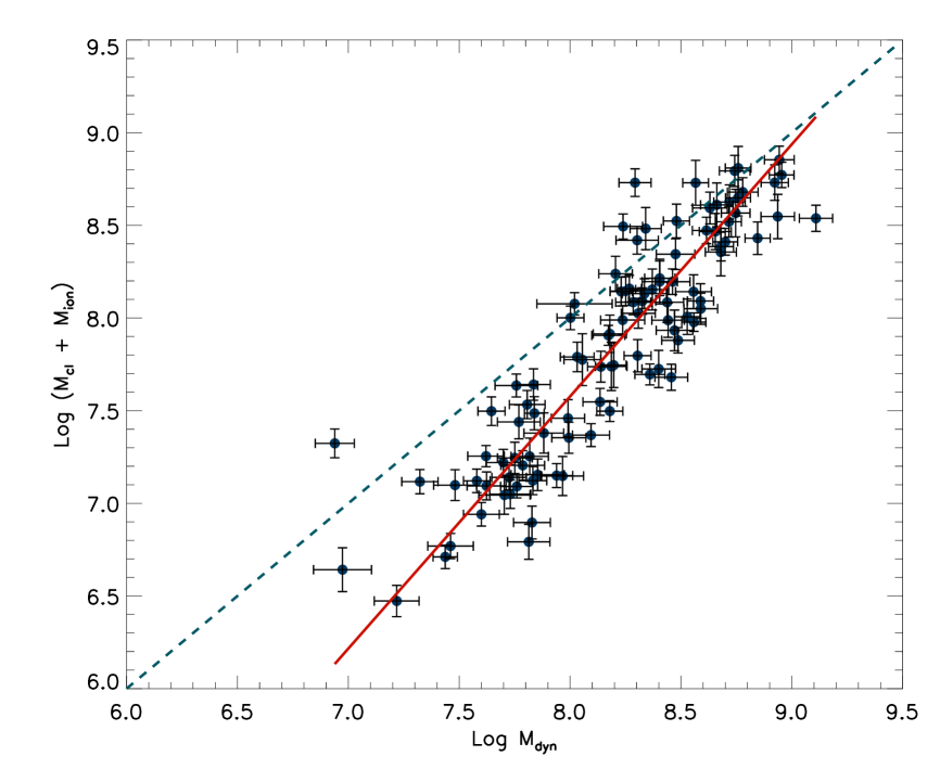
Figure 4.15: Comparison between $M_{cl}+M_{ion}$ and $M_{dyn}$. The continuos thick line represents the best fit to the data. The dashed line shows the one-to-one relation.

Dynamical masses

The dynamical masses were calculated following the expression (cf. Binney & Tremaine, 1987):

$$M_{dyn}=10^{3}R\sigma^{2},$$ (4.25)

where $\sigma$ is the velocity dispersion in $\mathrm{km\ s^{-1}}$, $M_{dyn}$ is given in $M_{\odot}$ and $R$ is the cluster effective radius in parsecs (i.e. such that $1/2$ of the mass lies inside it).

To obtain an unbiased estimate of the dynamical mass a good measurement of the effective size of the ionising massive cluster is necessary. As discussed above regarding the high dispersion observations, we have evidence that many of the objects in the sample are perhaps unresolved even under very good seeing conditions. We have searched the HST database for high resolution images of objects in our sample and found only 2 H ii galaxies with HST WFC3 images: J091434+470207 and J093813+542825.

A quick analysis of the HST images for these two objects shows that they are only marginally resolved and have effective radius of just a few parsecs. In order to improve the small number statistics we searched the HST high resolution database for star-forming nearby objects using the same selection criteria as for the objects in this chapter, and found 18 H ii galaxies and GEHR that also have SDSS images. Comparing the HST angular size with the Petrosian radius obtained from the SDSS u band photometry (corrected for seeing) we have found that the ionising cluster radius measured from the HST images is on average more than a factor of 5 smaller than the SDSS Petrosian radius. For estimating the dynamical mass we assumed that this factor applies to all H ii galaxies and therefore we have used a HST ‘corrected’ Petrosian radius as a proxy for the cluster radius. The values of the seeing corrected Petrosian to 50% of light radius are listed in column (11) of Table LABEL:tab:tab05. The calculated $M_{dyn}$ is given in column (12). The masses of the clusters, both photometric, i.e. $M_{cl}+M_{ion}$ and dynamical, are large and at the same time their size is very compact. The masses range over three decades from about 2 $\times$ 10⁶ M_⊙ to 10⁹ M_⊙ while the HST corrected Petrosian radius ranges from few tens of parsecs to a few hundred parsecs.

In Figure 4.15 we compare the sum of $M_{cl}+M_{ion}$ with $M_{dyn}$. It is clear from the figure that the value of $M_{dyn}$, computed assuming that the Petrosian radius is on average 5 times larger than the effective radius of the ionising cluster, is slightly larger than the sum of the photometric stellar and ionised gas components particularly for the lower mass objects. Also the fit to the data has a slope of 1.3 and not 1.0. Considering the uncertainties in the determination of the three parameters involved, the small level of the disagreement is surprising.

It is not clear at this stage what is the mass of the cold gas, both atomic and molecular, that remains from the starformation event. To further investigate this important question, in addition to high resolution optical and NIR images to measure the size of the ionizing clusters, high resolution observations in HI and CO or other molecular gas indicator are needed.

4.4.6 The metallicity – luminosity relation

In order to test the possible existence of a metallicity - luminosity relation for H ii galaxies, we have performed a least squares fit for the 100 objects with direct metallicity determination in the S3 sample using the continuum luminosity as calculated from the relation given by Terlevich & Melnick (1981) and the metallicity as calculated before. The results, shown in Figure 4.16, clearly indicate that a correlation exists albeit weak.

We have performed also a least squares fit using the H$\beta$ luminosity and the metallicity for the same sample. The results are shown in Figure 4.17 where a similarly weak correlation between both parameters can be seen.

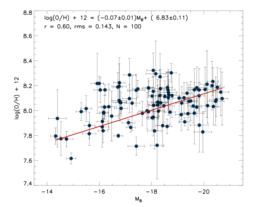
Figure 4.16: The continuum luminosity-metallicity relation for S3. The red line shows the best fit, which is described in the inset text.

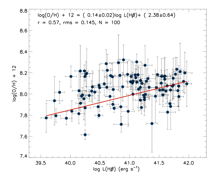
Figure 4.17: The $\mathrm{H}\beta$ luminosity-metallicity relation for S3. The red line shows the best fit, which is described in the inset text.

4.4.7 The metallicity – equivalent width relation

We tested the possibility that a relation exists between the metallicity and the equivalent width of the H$\beta$ emission line acting as a proxy for the age of the starburst. We have performed a least squares fit to these two parameters for the S3 sample. The results are shown in Figure 4.18 where a trend can be seen clearly. This correlation between EW$(\mathrm{H}\beta)$ and metallicity for a large sample of H ii galaxies covering a wider spectrum of ages and metallicities, has already been discussed in Terlevich et al. (2004) [see their Figure 5]. They interpreted the results as being consistent with two different timescales for the evolution of H ii galaxies on the metallicity – EW$(\mathrm{H}\beta)$ plane. The idea is that the observed value of the EW$(\mathrm{H}\beta)$ results from the emission produced in the present burst superposed on the continuum generated by the present burst plus all previous episodes of star formation that also contributed to enhance the metallicity.

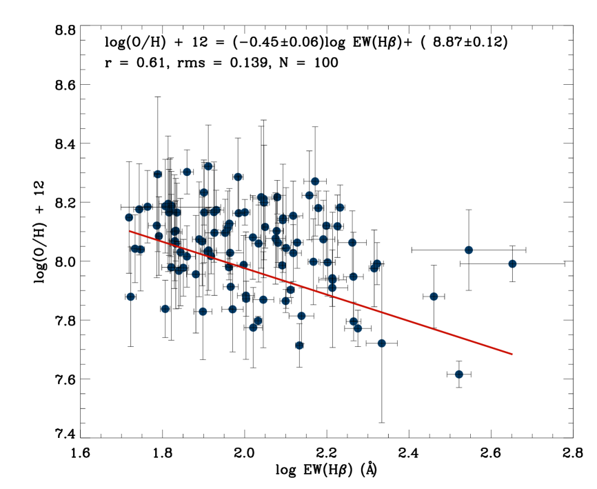
Figure 4.18: The EW($\mathrm{H}\beta$) - metallicity relation for S3. The red line shows the best fit, which is described in the inset text.

4.5 The L – $\sigma$ Correlation

The main objective of this chapter is to assess the validity of the $L-\sigma$ relation and its use as a distance estimator.

As discussed by e.g. Bordalo & Telles (2011), rotation and multiplicity of H ii regions in the sample objects can cause additional broadening of the emission lines which in turn may introduce scatter in the $L-\sigma$ relation.

In this context Chávez et al. (2012) performed a selection based on direct visual inspection of the H$\beta$, H$\alpha$ and [OIII]$\lambda\ 4959$ and $\lambda\ 5007$ line profiles combined with the kinematic analysis mentioned in §4.2.1. At the end of this process only 69 objects (subsample S5) of the observed 128 were left with symmetric gaussian profiles and no evidence of rotation or multiplicity. This turned up as being a very expensive process in terms of observing time.

4.5.1 Automatic profile classification

To evaluate objectively the ‘quality’ of the emission line profiles and to avoid possible biases associated with a subjective selection of the objects such as the ones performed by Bordalo & Telles (2011) or Chávez et al. (2012) we developed a blind testing algorithm that can ‘decide’ from the high dispersion data, which are the objects that have truly gaussian profiles in their emission lines. The algorithm uses $\delta_{FWHM}(\mathrm{H}\beta)<10$ and $\delta_{flux}(\mathrm{H}\beta)<10$ as selection criteria. These quantities are defined as follows:

$$\delta_{FWHM}=\frac{\Delta_{FWHM}}{\mu_{FWHM}}\times 100,$$ (4.26)

where $\mu_{FWHM}$ is the mean of the FWHM as measured from a single and triple gaussian fitting to a specific high resolution line profile and $\Delta_{FWHM}$ is the absolute value of the difference between these measurements. And

$$\delta_{flux}=\frac{\Delta_{flux}}{\mu_{flux}}\times 100,$$ (4.27)

where $\mu_{flux}$ is the mean of the fluxes as measured from the integration and gaussian fitting to the same spectral line in low resolution and $\Delta_{flux}$ is the absolute value of the difference between those measurements.

The rationale behind this approach is that these two quantities will measure departures from a single gaussian fitting of the actual profile. A large deviation is an indication of strong profile contamination due to second order effects such as large asymmetries and/or bright extended wings.

Figure 4.19 illustrates the parameters of the automatic selection. Objects inside the box delimited by a dashed line have $\delta_{flux}(\mathrm{H}\beta)<10$ and $\delta_{FWHM}(\mathrm{H}\beta)<10$. This, plus the condition $\log(\sigma)<1.8$, define the S4 sample of 93 objects.

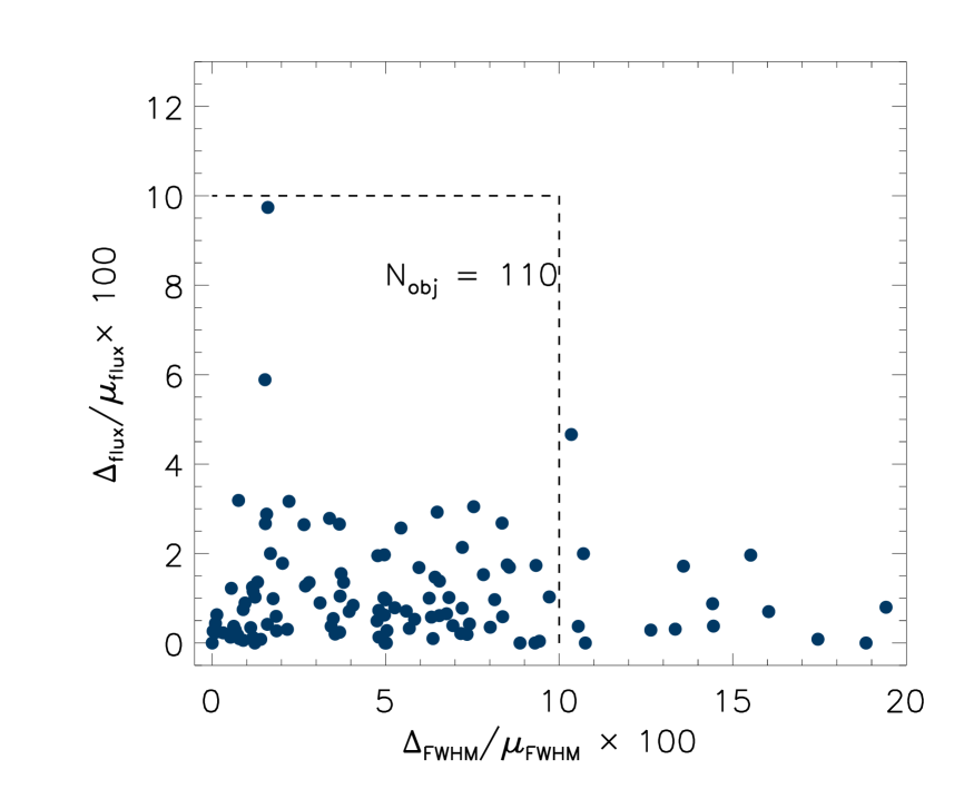
Figure 4.19: Automatic profile selection. Objects inside the box delimited by a dashed line have $\delta_{flux}(\mathrm{H}\beta)<10$ and $\delta_{FWHM}(\mathrm{H}\beta)<10$. This condition plus $\log(\sigma)<1.8$ define the S4 sample of 93 objects.

The $L-\sigma$ relation for the 107 objects in S3 for which we have a good estimate of their luminosity and velocity dispersion is shown in Figure 4.20. It follows the expression:

$$\log L(\mathrm{H}\beta)=(4.65\pm 0.14)\log\sigma+(33.71\pm 0.21),$$ (4.28)

with an rms scatter of $\delta\log L(\mathrm{H}\beta)=0.332$.

For the 69 objects of the restricted sample (S5) we obtained:

$$\log L(\mathrm{H}\beta)=(4.97\pm 0.17)\log\sigma+(33.22\pm 0.27),$$ (4.29)

An important conclusion of the comparison of the results obtained from S3 and S5 is that while the $L-\sigma$ relation scatter is reduced from an rms of 0.332 to an rms of 0.25 for S5, the errors in both the slope and zero points are slightly larger for the latter as a result of reducing the number of objects by about 2/3.

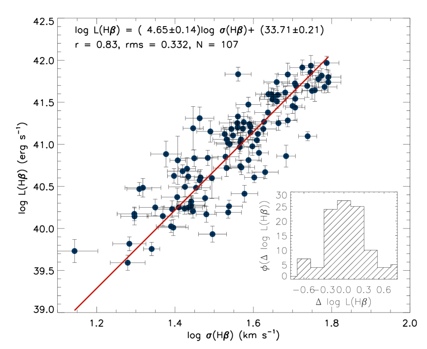
Figure 4.20: $L-\sigma$ relation for all the H ii galaxies with good determination of Luminosity and $\sigma$ (S3). The inset shows the distribution of the residuals of the fit.

4.5.2 Further restricting the sample by the quality of the line profile fits

We have also investigated the sensitivity of the $L(\mathrm{H}\beta)-\sigma$ relation to changes in the emission line profiles as determined by the quality of the gaussian fit. The definition of quality is related to the automatic profile classification described in the previous section and illustrated in Figure 4.19. As discussed previously, objects inside the box delimited by the dashed lines have $\delta_{flux}(\mathrm{H}\beta)<10$ and $\delta_{FWHM}(\mathrm{H}\beta)<10$. By adding the condition that $\log(\sigma)<1.8$ we obtain the S4 sample of 93 objects. We have selected five subsamples with increasing restricted definition of departure from a gaussian fit, i.e. with differences smaller than 10, 8, 5, 3 and 1 percent. The criteria are arbitrary and different cuts could have been justified, but the procedure was just used as a test and as such, any reasonable cut is valuable. The results of the fits are shown in Table 4.7.

Table 4.7: Correlation coefficients for the $L-\sigma$ relation for a range of discrimination levels in the automatic selection algorithm.

(1)	(2)	(3)	(4)	(5)
Cut Level	$\alpha$	$\beta$	rms	N
10	33.69 $\pm$ 0.22	4.67 $\pm$ 0.14	0.337	93
8	33.70 $\pm$ 0.23	4.66 $\pm$ 0.15	0.343	82
5	33.94 $\pm$ 0.26	4.51 $\pm$ 0.17	0.317	55
3	33.55 $\pm$ 0.33	4.74 $\pm$ 0.22	0.314	34
1	33.60 $\pm$ 0.49	4.63 $\pm$ 0.32	0.289	16

We can see from the table, that more restrictive gaussian selection still gives very similar values of the slope and the zero point of the $L(\mathrm{H}\beta)-\sigma$ relation. It achieves a small improvement in the rms but at the cost of a significantlly reduced sample which results in a substantial increase of the uncertainties of the slope and zero point roughly as the inverse of the square root of the number of objects.

It is interesting to compare these results with those using S3 with 107 objects some of them with profiles that clearly depart from gaussian. The least squares fit for S3 (see equation 4.36) gives coefficients $33.71\pm 0.21$ and $4.65\pm 0.14$ for the zero point and slope of the relation respectively. These values are very similar to those at the 10 percent cut but the rms and errors in the coefficients are smaller, consistent with a sample containing a larger number of objects.

The important conclusion from this exercise is that the $L(\mathrm{H}\beta)-\sigma$ relation is robust against profile selection. Selecting only those objects with the best gaussian profiles makes no change in the relation coefficients but substantially increases the uncertainties and the rms of the fit due to the reduction in the number of objects. We therefore strongly suggest the use of the $L(\mathrm{H}\beta)-\sigma$ relation without a finer line profile selection.

Furthermore, when applying the $L(\mathrm{H}\beta)-\sigma$ distance estimator to high redshift H ii galaxies where the data is bound to have a lower S/N, and a selection based on details of the emission line profile will be difficult to perform. Ideally we would like to reduce the distance estimator scatter without reducing the number of objects, i.e. with only a small percentage of rejects from the original observed sample.

Furthermore, it is clear from an inspection of Figure 4.20 (for S3) that the error bars are somehow smaller than the observed scatter in the relation, suggesting the presence of a second parameter in the correlation. As we will show below, this is indeed the case and thus it is possible to reduce substantially the scatter of the relation by including additional independent observables without a drastic reduction of the number of objects in the sample.

4.5.3 Search for a second parameter in the $L(\mathrm{H}\beta)-\sigma$ relation

In this section we explore the possibility that the scatter – at least part of it – in the $L(\mathrm{H}\beta)-\sigma$ relation is due to a second parameter.

Let us assume that the $L(\mathrm{H}\beta)-\sigma$ relation is a reflection of the virial theorem and a constant M/L ratio for the stellar population of these very young stellar clusters. Given that the virial theorem is bi-parametric, with the mass of the cluster depending on cluster’s velocity dispersion and size, one would expect the size of the system to be a second parameter in the $L(\mathrm{H}\beta)-\sigma$ relation.

The ionising flux in these young clusters evolve very rapidly, therefore it is also expected that age should play a role in the luminosity scatter. Thus parameters like the equivalent width of the Balmer lines or continuum colours, that are good age indicators, may also play a role in the scatter. Melnick et al. (1987) proposed chemical composition, in fact the oxygen abundance, as a second parameter in the $L(\mathrm{H}\beta)-\sigma$ relation.

In what follows we will analyse one by one these potential second parameters.

Table 4.8: Regression coefficients for S3

(1)	(2)	(3)	(4)	(5)	(6)
Parameter	$\alpha$	$\beta$	$\gamma$	rms	N
$R_{u}$	34.04 $\pm$ 0.20	3.08 $\pm$ 0.22	0.76 $\pm$ 0.13	0.261	99
$R_{g}$	34.29 $\pm$ 0.20	3.22 $\pm$ 0.22	0.59 $\pm$ 0.12	0.270	103
$R_{r}$	34.08 $\pm$ 0.21	3.29 $\pm$ 0.22	0.61 $\pm$ 0.13	0.274	101
$R_{i}$	34.08 $\pm$ 0.23	3.50 $\pm$ 0.22	0.50 $\pm$ 0.14	0.286	102
$R_{z}$	34.09 $\pm$ 0.23	3.36 $\pm$ 0.23	0.56 $\pm$ 0.14	0.282	101
$O/H$	32.16 $\pm$ 0.32	3.71 $\pm$ 0.22	0.38 $\pm$ 0.21	0.295	100
$N2$	35.60 $\pm$ 0.19	3.63 $\pm$ 0.24	0.21 $\pm$ 0.12	0.294	103
$R23$	34.47 $\pm$ 0.24	3.85 $\pm$ 0.23	0.59 $\pm$ 0.46	0.300	102
$W(H\beta)$	34.74 $\pm$ 0.23	3.73 $\pm$ 0.22	0.22 $\pm$ 0.15	0.303	107
$(u-i)$	35.08 $\pm$ 0.21	3.76 $\pm$ 0.22	0.05 $\pm$ 0.07	0.302	103

Table 4.9: Regression coefficients for S4.

(1)	(2)	(3)	(4)	(5)	(6)
Parameter	$\alpha$	$\beta$	$\gamma$	rms	N
$R_{u}$	34.08 $\pm$ 0.20	2.96 $\pm$ 0.25	0.81 $\pm$ 0.14	0.260	88
$R_{g}$	34.33 $\pm$ 0.20	3.07 $\pm$ 0.25	0.65 $\pm$ 0.13	0.268	90
$R_{r}$	34.09 $\pm$ 0.22	3.18 $\pm$ 0.25	0.67 $\pm$ 0.14	0.274	89
$R_{i}$	33.98 $\pm$ 0.23	3.33 $\pm$ 0.25	0.62 $\pm$ 0.17	0.285	89
$R_{z}$	34.13 $\pm$ 0.24	3.31 $\pm$ 0.25	0.57 $\pm$ 0.16	0.285	89
$O/H$	32.30 $\pm$ 0.33	3.71 $\pm$ 0.24	0.36 $\pm$ 0.24	0.298	87
$N2$	35.59 $\pm$ 0.20	3.63 $\pm$ 0.27	0.19 $\pm$ 0.14	0.299	89
$R23$	34.56 $\pm$ 0.25	3.85 $\pm$ 0.25	0.49 $\pm$ 0.50	0.304	89
$W(H\beta)$	34.77 $\pm$ 0.24	3.75 $\pm$ 0.24	0.19 $\pm$ 0.18	0.308	93
$(u-i)$	35.09 $\pm$ 0.22	3.77 $\pm$ 0.23	0.03 $\pm$ 0.08	0.305	90

Table 4.10: Bayesian Regression coefficients for S3

(1)	(2)	(3)	(4)	(5)	(6)
Parameter	$\alpha$	$\beta$	$\gamma$	rms	N
$R_{u}$	33.75 $\pm$ 0.37	3.36 $\pm$ 0.26	0.71 $\pm$ 0.14	0.263	99
$R_{g}$	33.84 $\pm$ 0.37	3.47 $\pm$ 0.25	0.61 $\pm$ 0.13	0.273	103
$R_{r}$	33.71 $\pm$ 0.41	3.57 $\pm$ 0.26	0.59 $\pm$ 0.14	0.277	101
$R_{i}$	33.61 $\pm$ 0.47	3.76 $\pm$ 0.25	0.52 $\pm$ 0.16	0.289	102
$R_{z}$	33.15 $\pm$ 0.46	3.47 $\pm$ 0.25	0.82 $\pm$ 0.17	0.290	101
$O/H$	30.67 $\pm$ 3.07	3.96 $\pm$ 0.26	0.51 $\pm$ 0.40	0.298	100
$N2$	34.94 $\pm$ 0.55	3.99 $\pm$ 0.28	0.14 $\pm$ 0.13	0.297	103
$R23$	33.83 $\pm$ 0.67	4.16 $\pm$ 0.26	0.75 $\pm$ 0.49	0.303	102
$W(H\beta)$	34.23 $\pm$ 0.51	4.02 $\pm$ 0.24	0.23 $\pm$ 0.17	0.305	107
$(u-i)$	34.62 $\pm$ 0.38	4.05 $\pm$ 0.24	0.04 $\pm$ 0.08	0.304	103

Size

If the $L(\mathrm{H}\beta)-\sigma$ correlation is a consequence of these young massive clusters being at (or close to) virial equilibrium, then the strongest candidate for a second parameter is the size of the star forming region (Terlevich & Melnick, 1981; Melnick et al., 1987). We have explored this possibility using the SDSS measured radii for our sample in all the available bands. The general form of the correlation is:

$$\log L(\mathrm{H}\beta)=\alpha+\beta\log\sigma+\gamma\log R_{i}\,$$ (4.30)

where $\alpha$, $\beta$ and $\gamma$ are the correlation coefficients and i runs over the SDSS bands (u, g, r, i, z). In all cases we have used the SDSS measured effective Petrosian radii and corrected for seeing also available from SDSS. Tables 4.8 and 4.9 show the correlation coefficients and the scatter obtained by means of a $\chi^{2}$ reduction procedure for the S3 and S4 samples respectively.

Consistent with what we found above regarding the profile selection, the results of the fits of the ‘10% cut’ sample S4 are not better than those of S3. Therefore in what follows we will only consider S3 taking it as the ‘benchmark’ sample.

Using the method proposed by Kelly (2007) and his publicly available IDL routines we performed also a bayesian multi-linear fit. The reason to use this additional analysis is to obtain better estimates of the uncertainties in every one of the correlation coefficients. The results of the analysis are shown in table 4.10 for S3. Comparing these results with those obtained previously (Tables 4.8 and 4.9) it is clear that there are only small differences in the coefficients and their uncertainties which are attributable to the better treatment of errors in the bayesian procedure. The bayesian zero point tends to be smaller while the slopes tend to be slightly larger.

Since at high redshifts the O[III]$\lambda$ 5007 line must be easier to observe than the H$\beta$ line, we have repeated the previous analysis using the values of velocity dispersion as measured from the O[III]$\lambda$ 5007 line instead of that of the $\mathrm{H}\beta$ line. The results for S3 are shown in Tables 4.11 and 4.12 for the $\chi^{2}$ reduction and the bayesian analysis respectively. After comparing the results presented in tables 8 and 11 we found that the use of $\sigma$(O[III]) introduces only a small extra dispersion in the relation.

At this stage we conclude that the size is indeed a second parameter of the correlation and in particular the size in the u band shows the best results. The corresponding relation for the S3 sample is given by:

$$\begin{split}\log&L(\mathrm{H}\beta)=(3.08\pm 0.22)\log\sigma+(0.76\pm 0.13)\log(R_{u})+\\ &+(34.04\pm 0.20),\end{split}$$ (4.31)

with an rms scatter of $\delta\log L(\mathrm{H}\beta)=0.261$.

Still, we have to be aware that the contribution of the size to the reduction of the scatter of the correlation is limited probably due to the fact to be discussed in §5.7, that the Petrosian radius of H ii galaxies is not a good estimator of the cluster dimension, but instead a measure of the size of the whole system, but indeed the positive reduction of the scatter of the $L(\mathrm{H}\beta)-\sigma$ relation when using even this measure of size, indicates that there is a subtle relation between both sizes.

Metallicity

Terlevich & Melnick (1981) proposed that oxygen abundance is a good indicator of the long term evolution of the system. They proposed a simple ‘closed box’ chemical evolution model with many successive cycles of star formation in which, for each cycle, evolution is traced by the $EW(\mathrm{H}\beta)$ whereas the long term evolution of the system, spanning two or more cycles, could be traced by the oxygen abundance, which then becomes a plausible second parameter in the $L(\mathrm{H}\beta)-\sigma$ correlation. When metallicity is used as a second parameter the resulting correlation is given by:

$$\log L(\mathrm{H}\beta)=\alpha+\beta\log\sigma+\gamma[12+\log\mathrm{(O/H)}]\,$$ (4.32)

where $\alpha$, $\beta$ and $\gamma$ are the correlation coefficients shown in Tables 4.8, 4.9, 4.10, 4.11 and 4.12 following the same procedure as described in the previous section for the radii. It is clear that the metallicity plays a role as a second parameter albeit relatively small. We must not forget, though, that because of the nature of the sample objects, the dynamical range of metallicity is very narrow (see Figure 4.14), not enough to affect significantly the $L(\mathrm{H}\beta)-\sigma$ correlation.

Table 4.11: Regression coefficients for S3 using $\sigma([\mathrm{OIII}])$.

(1)	(2)	(3)	(4)	(5)	(6)
Parameter	$\alpha$	$\beta$	$\gamma$	rms	N
$R_{u}$	34.44 $\pm$ 0.17	2.78 $\pm$ 0.24	0.82 $\pm$ 0.14	0.290	99
$R_{g}$	34.77 $\pm$ 0.16	2.93 $\pm$ 0.24	0.61 $\pm$ 0.13	0.303	103
$R_{r}$	34.55 $\pm$ 0.17	3.00 $\pm$ 0.24	0.64 $\pm$ 0.14	0.306	101
$R_{i}$	34.67 $\pm$ 0.18	3.23 $\pm$ 0.24	0.48 $\pm$ 0.16	0.321	102
$R_{z}$	34.53 $\pm$ 0.20	3.07 $\pm$ 0.24	0.60 $\pm$ 0.15	0.312	101
$O/H$	33.45 $\pm$ 0.24	3.45 $\pm$ 0.23	0.28 $\pm$ 0.23	0.328	100
$N2$	36.33 $\pm$ 0.15	3.28 $\pm$ 0.25	0.26 $\pm$ 0.14	0.327	103
$R23$	35.35 $\pm$ 0.18	3.52 $\pm$ 0.24	0.29 $\pm$ 0.50	0.332	102
$W(H\beta)$	35.02 $\pm$ 0.20	3.46 $\pm$ 0.23	0.35 $\pm$ 0.17	0.329	107
$(u-i)$	35.64 $\pm$ 0.17	3.51 $\pm$ 0.23	-0.02 $\pm$ 0.08	0.334	103

Table 4.12: Bayesian regression coefficients for S3 using $\sigma([\mathrm{OIII}])$.

(1)	(2)	(3)	(4)	(5)	(6)
Parameter	$\alpha$	$\beta$	$\gamma$	rms	N
$R_{u}$	34.29 $\pm$ 0.40	2.95 $\pm$ 0.27	0.78 $\pm$ 0.16	0.291	99
$R_{g}$	34.46 $\pm$ 0.39	3.08 $\pm$ 0.27	0.64 $\pm$ 0.15	0.304	103
$R_{r}$	34.34 $\pm$ 0.44	3.16 $\pm$ 0.27	0.62 $\pm$ 0.16	0.307	101
$R_{i}$	34.37 $\pm$ 0.50	3.40 $\pm$ 0.26	0.49 $\pm$ 0.18	0.322	102
$R_{z}$	33.75 $\pm$ 0.50	3.08 $\pm$ 0.26	0.85 $\pm$ 0.19	0.317	101
$O/H$	31.87 $\pm$ 3.41	3.57 $\pm$ 0.27	0.45 $\pm$ 0.44	0.330	100
$N2$	35.94 $\pm$ 0.56	3.49 $\pm$ 0.28	0.22 $\pm$ 0.15	0.328	103
$R23$	34.92 $\pm$ 0.71	3.72 $\pm$ 0.26	0.42 $\pm$ 0.54	0.333	102
$W(H\beta)$	34.72 $\pm$ 0.55	3.65 $\pm$ 0.24	0.35 $\pm$ 0.19	0.331	107
$(u-i)$	35.35 $\pm$ 0.38	3.70 $\pm$ 0.25	-0.03 $\pm$ 0.09	0.335	103

We have repeated the analysis using the strong line metallicity indicators N2 and R23. The results are also given in Tables 4.8, 4.9, 4.10, 4.11 and 4.12. They are similar to those obtained using T_e based direct metallicity but surprisingly, showing slightly less dispersion when using N2.

Age

The age of the starburst is also a second parameter candidate for the $L(\mathrm{H}\beta)-\sigma$ correlation. We used the $EW(\mathrm{H}\beta)$ as a starburst age indicator (Dottori, 1981; Dottori & Bica, 1981). The resulting correlation is given as:

$$\log L(\mathrm{H}\beta)=\alpha+\beta\log\sigma+\gamma\log EW(\mathrm{H}\beta)\,$$ (4.33)

and the coefficients are shown in Tables 4.8, 4.9, 4.10, 4.11 and 4.12.

Another possible age indicator is the continuum colour. We consider the (u - i) colour as a second parameter, the resulting correlation is given by:

$$\log L(\mathrm{H}\beta)=\alpha+\beta\log\sigma+\gamma(u-i)\,$$ (4.34)

The coefficients are also shown in Tables 4.8, 4.9, 4.10, 4.11 and 4.12.

From the above results, it is clear that age should play a role in the scatter of the $L(\mathrm{H}\beta)-\sigma$ correlation albeit very small. As with metallicity, by design the sample covers a narrow dynamic range of ages, consequence of the selection of equivalent widths of the emission lines, chosen such that only bursts younger than about 5 Myr are used in our study.

As already mentioned, we find that limiting the sample to objects with gaussian profiles does not improve the fit but limiting the sample to objects with log($\sigma$) $<$ 1.8, does. The second parameter with largest variance is the u size. Including it does improve radically the fit.

It is interesting to note that in the absence of a size determination, the best second parameter is the oxygen abundance O/H (or its proxy N2 or R23) in line with the early results of Terlevich & Melnick (1981); Melnick et al. (1987); Melnick, Terlevich & Moles (1988). This result is critical for future work with very distant systems where the Petrosian radius will be difficult to determine.

We therefore conclude that the best second parameter is the size in particular $R_{u}$. The use of the other observables [O/H, N2, R23, EW(H$\beta$), and (u - i)] also lead to a reduction of the scatter in the relation but to a lesser extent than what is achieved by using the size. Still they are useable in the absence of a size determination.

4.5.4 Multiparametric fits

The theoretical expectation that the emitted luminosity per unit mass in a young cluster should rapidly evolve with age and should also have some dependence on the metallicity of the stars, suggests that more parameters (other than the velocity dispersion and size of the cluster, e.g. its mass) may be playing a role in the $L(\mathrm{H}\beta)-\sigma$ relation.

We have explored the possibility that a third or even a fourth parameter are present in the correlation; the general expression for the fit is:

$$\log L(\mathrm{H}\beta)=\alpha+\beta\log\sigma+\gamma A+\delta B+\epsilon C\,$$ (4.35)

where $\alpha$, $\beta$, $\gamma$, $\delta$ and $\epsilon$ are the correlation coefficients and A, B and C are different combinations of parameters. Tables 4.13 and 4.14 show the parameter combinations that give the least scatter in the multi-parametric correlation for the sample S3 for a $\chi^{2}$ and a Bayesian methodology respectively. Tables 4.15 and 4.16 show the results when using the [OIII]$\lambda$ 5007 velocity dispersion.

A summary of the results indicates that when the $L(\mathrm{H}\beta)-\sigma$ relation is combined with the radius in the u band, the $(u-i)$ colour and the metallicity, the scatter is significantly reduced. The best result is:

$$\begin{split}\log&L(\mathrm{H}\beta)=(2.79\pm 0.23)\log\sigma+(0.95\pm 0.13)\log R_{u}+\\ +(&0.63\pm 0.19)\log EW(H\beta)+(0.28\pm 0.13)\log N2+\\ +(&33.15\pm 0.22),\end{split}$$ (4.36)

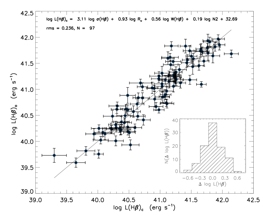
Figure 4.21: Observed L(H$\beta$) [L(H$\beta)_{o}$] vs. L(H$\beta$) calculated using the best Bayesian multi-parametric fitting corresponding to the expression displayed on the top of the figure. The 1:1 line is shown. The inset panel shows the luminosity residuals distribution.

with an rms scatter of $\delta\log L(\mathrm{H}\beta)=0.233$. This best solution is illustrated in Figure 4.21.

Table 4.13: Regression coefficients for S3.

(1)	(2)	(3)	(4)	(5)	(6)	(7)	(8)
Parameters	$\alpha$	$\beta$	$\gamma$	$\delta$	$\epsilon$	rms	N
$R_{u}$, $(u-i)$	33.93 $\pm$ 0.20	2.97 $\pm$ 0.22	0.91 $\pm$ 0.14	-0.16 $\pm$ 0.08	—	0.255	99
$R_{u}$, $O/H$	32.76 $\pm$ 0.24	3.10 $\pm$ 0.22	0.71 $\pm$ 0.13	0.17 $\pm$ 0.19	—	0.260	96
$R_{u}$, $N2$	33.73 $\pm$ 0.21	3.08 $\pm$ 0.22	0.88 $\pm$ 0.13	0.01 $\pm$ 0.11	—	0.247	97
$R_{u}$, $R23$	32.96 $\pm$ 0.24	3.20 $\pm$ 0.23	0.80 $\pm$ 0.13	0.91 $\pm$ 0.42	—	0.256	98
$R_{u}$, $W(H\beta)$	32.87 $\pm$ 0.23	3.00 $\pm$ 0.22	0.90 $\pm$ 0.13	0.47 $\pm$ 0.16	—	0.250	99
$W(H\beta)$, $O/H$	30.63 $\pm$ 0.38	3.69 $\pm$ 0.22	0.26 $\pm$ 0.17	0.51 $\pm$ 0.22	—	0.291	100
$W(H\beta)$, $N2$	35.38 $\pm$ 0.19	3.42 $\pm$ 0.26	0.43 $\pm$ 0.20	0.42 $\pm$ 0.16	—	0.288	103
$W(H\beta)$, $R23$	34.46 $\pm$ 0.24	3.83 $\pm$ 0.23	0.05 $\pm$ 0.19	0.51 $\pm$ 0.54	—	0.300	102
$R_{u}$, $(u-i)$, $O/H$	30.43 $\pm$ 0.31	2.90 $\pm$ 0.23	0.90 $\pm$ 0.14	-0.25 $\pm$ 0.09	0.46 $\pm$ 0.21	0.249	96
$R_{u}$, $(u-i)$, $N2$	34.17 $\pm$ 0.19	2.85 $\pm$ 0.25	0.99 $\pm$ 0.14	-0.19 $\pm$ 0.09	0.17 $\pm$ 0.13	0.241	97
$R_{u}$, $(u-i)$, $R23$	33.07 $\pm$ 0.23	3.09 $\pm$ 0.23	0.91 $\pm$ 0.14	-0.13 $\pm$ 0.08	0.75 $\pm$ 0.43	0.252	98
$R_{u}$, $W(H\beta)$, $O/H$	29.30 $\pm$ 0.33	2.95 $\pm$ 0.22	0.85 $\pm$ 0.13	0.57 $\pm$ 0.17	0.44 $\pm$ 0.19	0.244	96
$R_{u}$, $W(H\beta)$, $N2$	33.15 $\pm$ 0.22	2.79 $\pm$ 0.23	0.95 $\pm$ 0.13	0.63 $\pm$ 0.19	0.28 $\pm$ 0.13	0.233	97
$R_{u}$, $W(H\beta)$, $R23$	32.53 $\pm$ 0.25	3.07 $\pm$ 0.23	0.89 $\pm$ 0.13	0.39 $\pm$ 0.17	0.45 $\pm$ 0.46	0.249	98

Table 4.14: Bayesian Regression coefficients for S3.

(1)	(2)	(3)	(4)	(5)	(6)	(7)	(8)
Parameters	$\alpha$	$\beta$	$\gamma$	$\delta$	$\epsilon$	rms	N
$R_{u}$, $(u-i)$	33.60 $\pm$ 0.37	3.21 $\pm$ 0.26	0.90 $\pm$ 0.16	-0.18 $\pm$ 0.08	—	0.257	99
$R_{u}$, $O/H$	32.27 $\pm$ 2.77	3.38 $\pm$ 0.27	0.65 $\pm$ 0.15	0.20 $\pm$ 0.37	—	0.262	96
$R_{u}$, $N2$	33.16 $\pm$ 0.57	3.41 $\pm$ 0.26	0.85 $\pm$ 0.14	-0.07 $\pm$ 0.12	—	0.250	97
$R_{u}$, $R23$	32.40 $\pm$ 0.67	3.50 $\pm$ 0.26	0.77 $\pm$ 0.14	1.11 $\pm$ 0.45	—	0.258	98
$R_{u}$, $W(H\beta)$	32.46 $\pm$ 0.56	3.24 $\pm$ 0.25	0.87 $\pm$ 0.15	0.52 $\pm$ 0.17	—	0.251	99
$W(H\beta)$, $O/H$	27.89 $\pm$ 3.96	3.89 $\pm$ 0.27	0.38 $\pm$ 0.24	0.78 $\pm$ 0.47	—	0.295	100
$W(H\beta)$, $N2$	34.77 $\pm$ 0.54	3.81 $\pm$ 0.31	0.36 $\pm$ 0.25	0.31 $\pm$ 0.18	—	0.291	103
$W(H\beta)$, $R23$	33.84 $\pm$ 0.67	4.14 $\pm$ 0.26	0.02 $\pm$ 0.21	0.71 $\pm$ 0.57	—	0.303	102
$R_{u}$, $(u-i)$, $O/H$	26.05 $\pm$ 4.61	2.96 $\pm$ 0.35	0.95 $\pm$ 0.19	-0.42 $\pm$ 0.18	0.99 $\pm$ 0.60	0.260	96
$R_{u}$, $(u-i)$, $N2$	33.53 $\pm$ 0.62	3.20 $\pm$ 0.29	0.95 $\pm$ 0.15	-0.15 $\pm$ 0.10	0.06 $\pm$ 0.15	0.244	97
$R_{u}$, $(u-i)$, $R23$	32.48 $\pm$ 0.67	3.38 $\pm$ 0.27	0.89 $\pm$ 0.16	-0.14 $\pm$ 0.09	0.97 $\pm$ 0.45	0.255	98
$R_{u}$, $W(H\beta)$, $O/H$	27.19 $\pm$ 3.39	3.14 $\pm$ 0.27	0.82 $\pm$ 0.15	0.69 $\pm$ 0.23	0.65 $\pm$ 0.40	0.248	96
$R_{u}$, $W(H\beta)$, $N2$	32.69 $\pm$ 0.57	3.11 $\pm$ 0.28	0.93 $\pm$ 0.14	0.56 $\pm$ 0.22	0.19 $\pm$ 0.16	0.236	97
$R_{u}$, $W(H\beta)$, $R23$	31.97 $\pm$ 0.68	3.34 $\pm$ 0.27	0.87 $\pm$ 0.15	0.40 $\pm$ 0.20	0.66 $\pm$ 0.50	0.252	98

Table 4.15: Regression coefficients for S3 using $\sigma([\mathrm{OIII}])$.

(1)	(2)	(3)	(4)	(5)	(6)	(7)	(8)
Parameters	$\alpha$	$\beta$	$\gamma$	$\delta$	$\epsilon$	rms	N
$R_{u}$, $(u-i)$	34.21 $\pm$ 0.18	2.67 $\pm$ 0.23	1.03 $\pm$ 0.15	-0.26 $\pm$ 0.08	—	0.276	99
$R_{u}$, $O/H$	33.84 $\pm$ 0.19	2.81 $\pm$ 0.24	0.77 $\pm$ 0.15	0.09 $\pm$ 0.21	—	0.290	96
$R_{u}$, $N2$	34.40 $\pm$ 0.17	2.72 $\pm$ 0.24	0.90 $\pm$ 0.15	0.08 $\pm$ 0.13	—	0.280	97
$R_{u}$, $R23$	33.81 $\pm$ 0.19	2.85 $\pm$ 0.24	0.83 $\pm$ 0.14	0.56 $\pm$ 0.47	—	0.288	98
$R_{u}$, $W(H\beta)$	32.91 $\pm$ 0.22	2.73 $\pm$ 0.22	0.98 $\pm$ 0.14	0.60 $\pm$ 0.17	—	0.273	99
$W(H\beta)$, $O/H$	31.18 $\pm$ 0.33	3.43 $\pm$ 0.23	0.39 $\pm$ 0.18	0.47 $\pm$ 0.25	—	0.320	100
$W(H\beta)$, $N2$	35.79 $\pm$ 0.17	3.02 $\pm$ 0.25	0.71 $\pm$ 0.21	0.59 $\pm$ 0.16	—	0.309	103
$W(H\beta)$, $R23$	35.20 $\pm$ 0.19	3.49 $\pm$ 0.24	0.30 $\pm$ 0.20	-0.15 $\pm$ 0.58	—	0.328	102
$R_{u}$, $(u-i)$, $O/H$	30.45 $\pm$ 0.29	2.60 $\pm$ 0.23	1.02 $\pm$ 0.15	-0.35 $\pm$ 0.09	0.50 $\pm$ 0.23	0.269	96
$R_{u}$, $(u-i)$, $N2$	35.03 $\pm$ 0.16	2.41 $\pm$ 0.24	1.08 $\pm$ 0.15	-0.35 $\pm$ 0.09	0.35 $\pm$ 0.14	0.260	97
$R_{u}$, $(u-i)$, $R23$	33.90 $\pm$ 0.19	2.71 $\pm$ 0.24	1.03 $\pm$ 0.15	-0.25 $\pm$ 0.08	0.30 $\pm$ 0.46	0.275	98
$R_{u}$, $W(H\beta)$, $O/H$	29.98 $\pm$ 0.30	2.69 $\pm$ 0.23	0.93 $\pm$ 0.14	0.68 $\pm$ 0.18	0.37 $\pm$ 0.21	0.269	96
$R_{u}$, $W(H\beta)$, $N2$	33.40 $\pm$ 0.20	2.42 $\pm$ 0.23	0.98 $\pm$ 0.14	0.90 $\pm$ 0.20	0.45 $\pm$ 0.14	0.253	97
$R_{u}$, $W(H\beta)$, $R23$	33.04 $\pm$ 0.21	2.72 $\pm$ 0.23	0.96 $\pm$ 0.14	0.60 $\pm$ 0.19	-0.10 $\pm$ 0.49	0.273	98

Table 4.16: Bayesian regression coefficients for S3 and using $\sigma([\mathrm{OIII}])$.

(1)	(2)	(3)	(4)	(5)	(6)	(7)	(8)
Parameters	$\alpha$	$\beta$	$\gamma$	$\delta$	$\epsilon$	rms	N
$R_{u}$, $(u-i)$	34.03 $\pm$ 0.39	2.83 $\pm$ 0.26	1.02 $\pm$ 0.17	-0.29 $\pm$ 0.09	—	0.277	99
$R_{u}$, $O/H$	33.42 $\pm$ 3.08	2.96 $\pm$ 0.28	0.73 $\pm$ 0.17	0.12 $\pm$ 0.41	—	0.290	96
$R_{u}$, $N2$	34.04 $\pm$ 0.63	2.92 $\pm$ 0.27	0.89 $\pm$ 0.17	0.02 $\pm$ 0.14	—	0.281	97
$R_{u}$, $R23$	33.50 $\pm$ 0.71	3.03 $\pm$ 0.27	0.80 $\pm$ 0.16	0.70 $\pm$ 0.49	—	0.289	98
$R_{u}$, $W(H\beta)$	32.68 $\pm$ 0.63	2.85 $\pm$ 0.25	0.97 $\pm$ 0.16	0.63 $\pm$ 0.19	—	0.273	99
$W(H\beta)$, $O/H$	28.57 $\pm$ 4.40	3.52 $\pm$ 0.28	0.50 $\pm$ 0.26	0.75 $\pm$ 0.52	—	0.323	100
$W(H\beta)$, $N2$	35.39 $\pm$ 0.57	3.23 $\pm$ 0.30	0.72 $\pm$ 0.26	0.55 $\pm$ 0.19	—	0.310	103
$W(H\beta)$, $R23$	34.77 $\pm$ 0.71	3.69 $\pm$ 0.26	0.29 $\pm$ 0.23	0.02 $\pm$ 0.62	—	0.329	102
$R_{u}$, $(u-i)$, $O/H$	24.62 $\pm$ 5.03	2.53 $\pm$ 0.35	1.10 $\pm$ 0.20	-0.57 $\pm$ 0.19	1.23 $\pm$ 0.65	0.286	96
$R_{u}$, $(u-i)$, $N2$	34.68 $\pm$ 0.62	2.60 $\pm$ 0.28	1.08 $\pm$ 0.17	-0.36 $\pm$ 0.11	0.30 $\pm$ 0.16	0.261	97
$R_{u}$, $(u-i)$, $R23$	33.52 $\pm$ 0.69	2.88 $\pm$ 0.27	1.03 $\pm$ 0.17	-0.27 $\pm$ 0.09	0.46 $\pm$ 0.49	0.276	98
$R_{u}$, $W(H\beta)$, $O/H$	27.64 $\pm$ 3.87	2.73 $\pm$ 0.29	0.92 $\pm$ 0.17	0.80 $\pm$ 0.25	0.63 $\pm$ 0.46	0.272	96
$R_{u}$, $W(H\beta)$, $N2$	33.10 $\pm$ 0.62	2.56 $\pm$ 0.27	0.99 $\pm$ 0.16	0.89 $\pm$ 0.24	0.40 $\pm$ 0.17	0.254	97
$R_{u}$, $W(H\beta)$, $R23$	32.72 $\pm$ 0.73	2.85 $\pm$ 0.27	0.95 $\pm$ 0.16	0.62 $\pm$ 0.21	0.02 $\pm$ 0.53	0.274	98

It seems reasonable to infer that the resulting coefficients support the scenario of a virial origin of the $L(\mathrm{H}\beta)-\sigma$ relation, in that the $\log\sigma$ coefficient is smaller than 3, the size coefficient is close to 1 and that other effects like the age and metallicity of the burst alter the virial nature of the relation.

Table 4.17: Regression coefficients-HDS.

(1)	(2)	(3)	(4)	(5)	(6)	(7)	(8)
Parameters	$\alpha$	$\beta$	$\gamma$	$\delta$	$\epsilon$	rms	N
$R_{u}$, $(u-i)$, $O/H$	28.44	2.72	1.12	-0.23	0.66	0.256	55
$R_{u}$, $(u-i)$, $N2$	34.21	2.62	1.13	-0.19	0.25	0.258	57
$R_{u}$, $W(H\beta)$, $O/H$	27.37	2.81	1.03	0.72	0.61	0.240	57
$R_{u}$, $W(H\beta)$, $N2$	32.95	2.43	1.04	1.01	0.49	0.232	59

Table 4.18: Regression coefficients-UVES.

(1)	(2)	(3)	(4)	(5)	(6)	(7)	(8)
Parameters	$\alpha$	$\beta$	$\gamma$	$\delta$	$\epsilon$	rms	N
$R_{u}$, $(u-i)$, $O/H$	30.84	3.09	0.85	-0.18	0.38	0.199	38
$R_{u}$, $(u-i)$, $N2$	34.80	2.85	0.84	-0.22	0.30	0.209	38
$R_{u}$, $W(H\beta)$, $O/H$	33.23	3.02	0.53	0.13	0.16	0.232	39
$R_{u}$, $W(H\beta)$, $N2$	34.29	3.04	0.72	0.07	0.13	0.216	38

Comparing the scatter between UVES and HDS data

We discussed in §4.2.2 the different setups used for the HDS and UVES observations. We show in Tables 4.17 and 4.18 the regression coefficients calculated separately for both sets of observations and the combination of parameters that renders the least scatter.

It can be seen that the scatter of the HDS data is larger than that of the UVES data. We interpret this as an effect of the wider slit used in the HDS observations combined with the compact size of the sources and the excellent seeing prevailing during the observations. All these effects put together plus unavoidable fluctuations in the auto guiding procedure may have contributed in increasing the uncertainties in the observed emission line profiles.

Although a similar but smaller effect cannot at this stage be ruled out from the UVES data, given that the slit used was also larger than the seeing disk, we can conclude that the ‘true’ scatter of the relation is probably closer – if not even smaller – to that observed in the UVES data, i.e. r.m.s. $\lesssim$0.2.

4.6 Summary

We have carefully constructed a sample of 128 compact local H ii galaxies, with high equivalent widths of their Balmer emission lines, with the objective of assessing the validity of the $L({H\beta})-\sigma$ relation and its use as an accurate distance estimator. To this end we obtained high S/N high-dispersion ESO VLT and Subaru echelle spectroscopy, in order to accurately measure the ionized gas velocity dispersion. Additionally, we obtained integrated H$\beta$ fluxes from low dispersion wide aperture spectrophotometry, using the 2.1m telescopes at Cananea and San Pedro Mártir in Mexico, complemented with data from the SDSS spectroscopic survey.

After further restricting the sample to include only those systems with $\log\sigma<1.8$ and removing objects with low quality data, the remaining sample consists of 107 ‘bonafide’ H ii galaxies. These systems have indeed luminosities and metallicities typical of H ii galaxies and their position in the diagnostic diagram is typical of high excitation, low metallicity and extremely young H ii regions.

Using this sample we have found that:

1. The $L(\mathrm{H}\beta)-\sigma$ relation is strong and stable against changes in the sample definition, based on the characteristics of the emission line profiles. In particular we have investigated the role that the ‘gaussianity’ of the line profile plays on the relation. This was tested to destruction with both objective and subjective methods of profile classification and assessment to define several subsets.

   In agreement with previous work we find that the $L(\mathrm{H}\beta)-\sigma$ relation for H ii galaxies with gaussian emission line profiles has a smaller scatter than that of the complete sample. On the other hand this is achieved at the cost of substantially reducing the sample. The rejected fraction in Bordalo & Telles (2011) or Chávez et al. (2012) is close to or larger than 50%, which is not compensated by the gain in rms. The use of the complete sample, i.e. without a profile classification, is a far more practical proposal given that, in order to perform a proper selection of gaussian profiles, we need data that have S/N and resolution much higher than that required to measure just the FWHM. Therefore it is far more costly in terms of observing time and instrumentation requirements to determine departures from gaussianity than to just accurately measure the FWHM of an emission line. It is shown in section 4.5.2 that while the r.m.s. errors are indeed reduced on the fits to the subset of H ii galaxies with Gaussian profiles, the value of the coefficients hardly change at all, although their errors are substantially larger than those of the complete sample.

   In conclusion, selecting the best gaussian profiles improves the rms but at a very heavy cost in terms of rejects and hence of telescope time, which is neither practical nor justified for a distance estimator, as we showed in section 4.5.

   Therefore, the use of the full sample, limited only by the $\log\sigma<1.8$ selection, is strongly recommended. Our best $L(\mathrm{H}\beta)-\sigma$ relation is:

   $${\log L(\mathrm{H}\beta)=4.65\log\sigma+33.71\;,}$$

   with an rms scatter of ${\delta\log L(\mathrm{H}\beta)=0.332}$.

2. We searched for the presence of a second parameter in the $L(\mathrm{H}\beta)-\sigma$ relation. We found that using as second parameter either size, oxygen abundance O/H or its proxy N2 or R23, EW or continuum colour, the scatter is considerably reduced. Including the size as a second parameter produces the best fits, and among them the size in the u-band shows the smallest scatter,

   $$\log L(\mathrm{H}\beta)=3.08\log\sigma+0.76\log R_{u}+34.04\;,$$

   with an rms scatter of $\delta\log L(\mathrm{H}\beta)=0.261$.

   This result points clearly to the existence of a Fundamental Plane in H ii galaxies suggesting that the main mechanism of line broadening is linked to the gravitational potential of the young massive cluster. It is important to underline that in the absence of a size measurement, the best second parameter is the abundance O/H or its proxy N2 or R23, a result that is crucial for the application to very distant systems where the size will be difficult to determine.

3. We also investigated which parameters in addition to the size can further reduce the scatter. We found, using multi parametric fits , that including as a third parameter the $(u-i)$ colour or the equivalent width, and as a fourth parameter the metallicity does significantly reduce further the scatter.

   Our best multiparametric estimator is:
   

   $$\log L(\mathrm{H}\beta)=2.79\log\sigma+0.95\log R_{u}+0.63\log EW(H\beta)+$$

   $$0.28\log N2+33.15$$

   with an rms scatter of $\delta\log L(\mathrm{H}\beta)=0.233$.
   

   The argument could be sustained that the value of the coefficients of the fit provides further support for the virial origin of the $L(\mathrm{H}\beta)-\sigma$ relation since the $\log\sigma$ coefficient is smaller than 3. It is quite possible that such virial nature is altered by other effects like the age (EW) and metallicity (N2) of the burst. Thus the coefficients in the best estimator (see equation (4.36)) are very close to what is expected from a young virialized ionising cluster and, perhaps even more relevant, the sum of the stellar and ionised gas masses of the cluster are similar to the dynamical mass estimated with the HST ‘corrected’ Petrosian radius.

   We conclude that the evidence strongly points to gravity as the main mechanism for the broadening of the emission lines in these very young and massive clusters.

4. The masses of the clusters, both photometric and dynamical, are very large while their size is very compact. Their range covers three decades from about 2 $\times$ 10⁶ M_⊙  to 10⁹ M_⊙. Their HST corrected Petrosian radius range from a few tens of parsecs to a few hundred parsecs. To further investigate this important property of the H ii galaxies and its impact on the distance estimator it is crucial to secure high resolution optical and NIR images of this sample of objects.

5. Bayesian and $\chi^{2}$ fits to the $L(\mathrm{H}\beta)-\sigma$ correlation give similar results.

6. The application of the $L(\mathrm{H}\beta)-\sigma$ distance estimator to H ii galaxies at cosmological distances, where the size would be difficult to determine, will require the use of a metallicity indicator and the EW of the Balmer lines as a second and third parameter. According to our findings, this will result in a predictor with $\delta\log L(\mathrm{H}\beta)\sim 0.3$ using either $\sigma(H\beta)$ or the easier to determine, at such redshifts, $\sigma[OIII]$.

7. Given that the $L(\mathrm{H}\beta)-\sigma$ relation is basically a correlation between the ionising flux, produced by the massive stars, and the velocity field produced by the star and gas potential well, the existence of a narrow $L(\mathrm{H}\beta)-\sigma$ relation puts strong limits on the possible changes in the IMF. Any systematic variation in the IMF will affect directly the M/L ratio and therefore the slope and/or zero point of the relation. A change of 0.1 in the slope of the IMF would be reflected in a change in luminosity scale of the $L(\mathrm{H}\beta)-\sigma$ relation of about $\log L(\mathrm{H}\beta)\sim\ 0.2$. This seems to be too large for the derived correlation.

8. An important aspect to remark is that the design of our complete selection criteria guarantees homogeneous samples at all redshifts in the sense that the imposed EW limit guarantees a sample younger than a certain age and relatively free of contamination by older populations, the upper limit in $\sigma$ guarantees a sample limited in luminosity and the diagnostic diagram selection guarantees that they are starbursts. The limitation in $\sigma$ is particularly important given that this criterion should remove biases associated with samples in which the mean luminosity changes with distance (Malmquist bias). Any dependence of the luminosity in parameters like age and metallicity are included in the multiparametric fits.

   Finally, we envisage observations of H ii galaxies having a limiting $\sigma$ of 63 km/s or equivalently an $\mathrm{H}\alpha\$ luminosity less than $3\times 10^{43}$ erg/s at z $\sim$ 2 to 3 with enough S/N with present instrumentation. They will require exposure times of about 1.5 to 3 hours in an instrument like X-SHOOTER at the VLT in ESO to obtain line profiles with enough S/N to determine FWHM with less than 10% rms error. This in turn will allow us to measure the local expansion rate of the Universe, $H_{0}$, to a percent precision which is a prerequisite for independent constraints on the mass-energy content and age of the Universe as well as to map its behaviour by using several independent yet accurate tracers of the cosmic expansion over the widest possible range of redshift.

Chapter 5 The Hubble Constant

We have found a strange footprint on the shores of the unknown.

— Sir A. S. Eddington, Space, Time and Gravitation (1920)

The accurate determination of the Hubble constant, $H_{0}$, is considered one of the most fundamental tasks in the interface between Astronomy and Cosmology. The importance of measuring the expansion rate of the Universe to high precision stems from the fact that $H_{0}$, besides providing cosmic distances, is also a prerequisite for independent constraints on the mass-energy content of the Universe (e.g. Suyu et al., 2012).

The direct determination of the Hubble constant can only be obtained by measuring cosmic distances and mapping the local expansion of the Universe, since the Hubble relation, $cz=H_{0}d$, is valid and independent of the mass-energy content of the Universe only locally ($z\raise-3.0pt\hbox{\hbox to0.0pt{\hbox{$\sim$}\hss}\raise 4.0pt\hbox{$<$}\ }0.15$). A variety of methods have been used to estimate $H_{0}$, based on Cepheids, surface brightness fluctuations, masers, the tip of the red giant branch (TRGB), or type Ia supernovae (for general reviews see Jackson, 2007; Tammann, Sandage & Reindl, 2008; Freedman & Madore, 2010). In particular, the use of SNae Ia to measure the Hubble constant has a long history in astronomy (e.g. Sandage & Tammann, 1982, 1990). The subsequent discovery of the correlation between the magnitude at peak brightness and the rate at which it declines thereafter (e.g. Phillips, 1993) allowed the reduction of the distance determination intrinsic scatter. However, one has to remember that SNae Ia are secondary indicators and their use relies on the determination of well-established local calibrators, like the Large Magellanic Cloud (LMC), Galactic Cepheids, the “maser” galaxy NGC 4258, etc. (cf. Riess et al., 2011).

Indirect methods to measure $H_{0}$ have also been developed, based either on the physics of the hot X-ray emitting inter-cluster gas (Sunyaev-Zeldovich effect), providing values of $H_{0}=73.7\pm 4\pm 9$ km s^-1 Mpc^-1 (e.g. Birkinshaw, 1999; Carlstrom, Holder & Reese, 2002; Bonamente et al., 2006), or on gravitational lens time delays (e.g. Schechter, 2005; Oguri, 2007; Suyu et al., 2009) providing a wide range of $H_{0}$ values, with the latter study giving $H_{0}=71\pm 3$ km s^-1 Mpc^-1. In addition, strategies based on the physics of the Universe just prior to recombination have been proposed (CMB anisotropy and BAO; Spergel et al., 2007; Komatsu et al., 2011; Beutler et al., 2011, and references therein). However, the latter methods use as priors other cosmological parameters, and thus the resulting $H_{0}$ measurements are strongly model dependent.

Returning to the direct method to estimate $H_{0}$, an important breakthrough occurred a decade or so ago by the HST Calibration program (Saha et al., 2001; Sandage et al., 2006) who found Cepheids in local galaxies that host SNae Ia and provided a Cepheid based zero-point calibration, and by the HST Key project (Freedman et al., 2001) who furnished a value of $H_{0}=72\pm 2{\rm(random)}\pm 7{\rm(systematic)}$ km s^-1 Mpc^-1, based on Cepheid distances of external galaxies and the LMC as the first rung of the distance ladder. This value was recently revised by the same authors, using a new Cepheid zero-point (Benedict et al., 2007a) and the new SNae Ia of Hicken et al. (2009), to a similar but less uncertain value of $H_{0}=73\pm 2{\rm(random)}\pm 4{\rm(systematic)}$ km s^-1 Mpc^-1 (see Freedman & Madore, 2010). Tammann, Sandage & Reindl (2008) used a variety of local calibrators to recalibrate the SNae Ia and found a significantly lower value of $H_{0}=62.3\pm 4$ km s^-1Mpc^-1. The difference has since been explained as being due to a variety of external causes among which the use of heavily reddened Galactic Cepheids and of less accurate photographic data (Riess et al., 2009a, b).

The most recent analysis of Riess et al. (2011) uses new HST optical and infrared observations of 600 Cepheid variables to determine the distance to eight galaxies hosting recent SNae Ia. The resulting best estimate for the Hubble constant is: $H_{0}=73.8\pm 2.4$ km s^-1 Mpc^-1 (including random and systematic errors).

From the above discussion it becomes clear that SNae Ia are the only tracers of the Hubble expansion utilized to-date, over a relatively large redshift range ($0\raise-3.0pt\hbox{\hbox to0.0pt{\hbox{$\sim$}\hss}\raise 4.0pt\hbox{$<$}\ }z\raise-3.0pt\hbox{\hbox to0.0pt{\hbox{$\sim$}\hss}\raise 4.0pt\hbox{$<$}\ }0.1$). Therefore, due to the great importance of direct determinations of the Hubble constant for cosmological studies (e.g. Suyu et al., 2012) it is highly desirable to independently confirm the SNae Ia based $H_{0}$ value by using an alternative tracer.

H ii galaxies have been proposed as such an alternative, and a first attempt to estimate $H_{0}$, using giant H ii regions as local calibrators, was presented in Melnick, Terlevich & Moles (1988). Recently, we presented a thorough investigation of the viability of using H ii galaxies to constrain the dark energy equation of state, accounting also for the effects of gravitational lensing, which are expected to be non-negligible for very high redshift ‘standard candles’ and we showed that indeed H ii galaxies can represent an important cosmological probe (Plionis et al., 2011).

The aim of the current chapter is to use H ii galaxies and a local calibration of the $L(\mathrm{H}\beta)-\sigma$ relation based on giant H ii regions of nearby galaxies, as an alternative direct approach for estimating the Hubble constant over a redshift range of $0.01<z<0.16$. This chapter follows closely the work presented in Chávez et al. (2012).

5.1 Sample Selection and Observations

As described in the previous chapter, a sample of 128 H ii galaxies was selected from the SDSS DR7 spectroscopic data release (Abazajian et al., 2009) within a redshift range $0.01<z<0.16$, chosen for being compact ($D<5\ \mathrm{arcsec}$) having large Balmer emission line fluxes and equivalent widths. A lower limit for the equivalent width ($W$) of $\mathrm{H}\beta$ was chosen to avoid evolved starbursts, that would present underlying absorption components in their spectra due to an older stellar population component, thus affecting the emission line fluxes (cf. Melnick, Terlevich & Terlevich, 2000). The redshift lower limit was chosen to minimise the effects of local peculiar motions relative to the Hubble flow and the upper limit to minimise any possible Malmquist bias and avoid gross cosmological effects.

In order to improve the parameters of the $L(\mathrm{H}\beta)-\sigma$  relation obtained from previous work, high-resolution echelle spectroscopy for the H ii galaxy sample was performed with 8 meter class telescopes. To obtain accurate total $\mathrm{H}\beta$ fluxes for the H ii galaxy sample, we performed long slit spectrophotometry at 2-meter class telescopes under photometric conditions and using a slit width (8 arcsec) larger than the upper limit of the HII galaxies size in our sample.

$\mathrm{H}\beta$ and $[\mathrm{O\ III}]\ \lambda\lambda 4959,\ 5007$ line widths were measured by means of fitting single gaussians to the line profiles. H ii galaxies with peculiar line profiles due to double lines or rotation-broadened ones, were removed from the sample in order to avoid systematic errors in their $\mathrm{H}\beta$ luminosity determination. Our final sample of H ii galaxies was thus reduced from 128 to 69 galaxies (see also the discussion in chapter 4).

5.1.1 The anchor sample

The first step in the determination of $H_{0}$ is the determination of an accurate value of the zero point for the $L(\mathrm{H}\beta)-\sigma$ correlation. In order to do so, we need a sample for which independent distance determinations are available.

We have used a sample of 22 Giant Extragalactic H ii Regions (GEHR) located in 9 nearby galaxies for which distances can be estimated from alternative primary methods, fundamentally Cepheids, RR Lyrae and Eclipsing Binaries. We have reassessed the distance modulus for every object from the measurements reported in the literature since 1995. We have used weighted mean distance values. Table LABEL:tab:tab8 shows the values of the distance modulus for every object and the references from which it has been derived.

The values for integrated $\mathrm{H}\beta$ fluxes, velocity dispersion and absorption coefficients have been obtained from the results published by Melnick et al. (1987).

Table 5.1: Distance Moduli for the host galaxies of the GEHR sample.

(1)	(2)	(3)	(4)	(5)
Galaxy	$\mu$	$D$	Method	Reference
	(mag)	(kpc)
LMC	18.64 $\pm$ 0.02	53.46 $\pm$ 2.46	Cepheids	di Benedetto (1995)
	18.42 $\pm$ 0.11	48.31 $\pm$ 12.24	Cepheids	Bohm-Vitense (1997)
	18.57 $\pm$ 0.19	51.76 $\pm$ 22.64	RR Lyrae	Alcock et al. (1997)
	18.58 $\pm$ 0.02	52.00 $\pm$ 2.39	Cepheids	di Benedetto (1997)
	18.53 $\pm$ 0.04	50.82 $\pm$ 4.68	RR Lyrae	Feast (1997)
	18.26 $\pm$ 0.15	44.87 $\pm$ 15.50	RR Lyrae	Fernley et al. (1998)
	18.29 $\pm$ 0.17	45.50 $\pm$ 17.81	Cepheids	Luri et al. (1998)
	18.37 $\pm$ 0.23	47.21 $\pm$ 25.00	RR Lyrae	Luri et al. (1998)
	18.44 $\pm$ 0.35	48.75 $\pm$ 39.29	Cepheids	Madore & Freedman (1998)
	18.50 $\pm$ 0.13	50.12 $\pm$ 15.00	Cepheids	Madore & Freedman (1998)
	18.53 $\pm$ 0.14	50.82 $\pm$ 16.38	Cepheids	Madore & Freedman (1998)
	18.57 $\pm$ 0.11	51.76 $\pm$ 13.11	Cepheids	Madore & Freedman (1998)
	18.59 $\pm$ 0.15	52.24 $\pm$ 18.04	Cepheids	Madore & Freedman (1998)
	18.60 $\pm$ 0.15	52.48 $\pm$ 18.13	Cepheids	Madore & Freedman (1998)
	18.62 $\pm$ 0.18	52.97 $\pm$ 21.95	Cepheids	Madore & Freedman (1998)
	18.74 $\pm$ 0.24	55.98 $\pm$ 30.93	Cepheids	Madore & Freedman (1998)
	18.77 $\pm$ 0.24	56.75 $\pm$ 31.36	Cepheids	Madore & Freedman (1998)
	18.86 $\pm$ 0.36	59.16 $\pm$ 49.04	Cepheids	Madore & Freedman (1998)
	18.46 $\pm$ 0.02	49.20 $\pm$ 2.27	Cepheids	Gieren, Fouque & Gomez (1998)
	18.30 $\pm$ 0.07	45.71 $\pm$ 7.37	Eclipsing Binary	Guinan et al. (1998)
	18.35 $\pm$ 0.07	46.77 $\pm$ 7.54	Eclipsing Binary	Guinan et al. (1998)
	18.22 $\pm$ 0.13	44.06 $\pm$ 13.19	Eclipsing Binary	Udalski et al. (1998)
	18.61 $\pm$ 0.28	52.72 $\pm$ 33.99	RR Lyrae	Groenewegen & Salaris (1999)
	18.42 $\pm$ 0.30	48.31 $\pm$ 33.37	Cepheids	Bono et al. (1999)
	18.62 $\pm$ 0.12	52.97 $\pm$ 14.64	Cepheids	Bono et al. (1999)
	18.62 $\pm$ 0.17	52.97 $\pm$ 20.73	Cepheids	Bono et al. (1999)
	18.74 $\pm$ 0.13	55.98 $\pm$ 16.76	Cepheids	Bono et al. (1999)
	18.57 $\pm$ 0.05	51.76 $\pm$ 5.96	Cepheids	Sandage, Bell & Tripicco (1999)
	18.72 $\pm$ 0.09	55.46 $\pm$ 11.49	Cepheids	Feast (1999)
	18.52 $\pm$ 0.18	50.58 $\pm$ 20.96	Cepheids	Groenewegen & Oudmaijer (2000)
	18.54 $\pm$ 0.19	51.05 $\pm$ 22.33	Cepheids	Groenewegen & Oudmaijer (2000)
	18.60 $\pm$ 0.11	52.48 $\pm$ 13.29	Cepheids	Groenewegen & Oudmaijer (2000)
	18.66 $\pm$ 0.15	53.95 $\pm$ 18.63	Cepheids	Groenewegen & Oudmaijer (2000)
	18.52 $\pm$ 0.02	50.58 $\pm$ 2.33	RR Lyrae	Kovács (2000a)
	18.40 $\pm$ 0.07	47.86 $\pm$ 7.71	Eclipsing Binary	Nelson et al. (2000)
	18.42 $\pm$ 0.10	48.31 $\pm$ 11.12	Cepheids	Gieren et al. (2000)
	18.50 $\pm$ 0.13	50.12 $\pm$ 15.00	Cepheids	Ferrarese et al. (2000)
	18.42 $\pm$ 0.08	48.31 $\pm$ 8.90	Eclipsing Binary	Groenewegen & Salaris (2001)
	18.46 $\pm$ 0.06	49.20 $\pm$ 6.80	Eclipsing Binary	Groenewegen & Salaris (2001)
	18.42 $\pm$ 0.24	48.31 $\pm$ 26.69	Eclipsing Binary	Salaris & Groenewegen (2002)
	18.43 $\pm$ 0.24	48.53 $\pm$ 26.82	Eclipsing Binary	Salaris & Groenewegen (2002)
	18.35 $\pm$ 0.03	46.77 $\pm$ 3.23	Cepheids	Paturel et al. (2002)
	18.37 $\pm$ 0.14	47.21 $\pm$ 15.22	Cepheids	Paturel et al. (2002)
	18.38 $\pm$ 0.10	47.42 $\pm$ 10.92	RR Lyrae	Benedict & et al. (2002b)
	18.53 $\pm$ 0.10	50.82 $\pm$ 11.70	RR Lyrae	Benedict & et al. (2002b)
	18.50 $\pm$ 0.13	50.12 $\pm$ 15.00	Cepheids	Benedict & et al. (2002a)
	18.58 $\pm$ 0.15	52.00 $\pm$ 17.96	Cepheids	Benedict & et al. (2002a)
	18.31 $\pm$ 0.10	45.92 $\pm$ 10.57	Eclipsing Binary	Fitzpatrick et al. (2002)
	18.36 $\pm$ 0.10	46.99 $\pm$ 10.82	Eclipsing Binary	Fitzpatrick et al. (2002)
	18.50 $\pm$ 0.06	50.12 $\pm$ 6.92	Eclipsing Binary	Fitzpatrick et al. (2002)
	18.52 $\pm$ 0.06	50.58 $\pm$ 6.99	Eclipsing Binary	Fitzpatrick et al. (2002)
	18.53 $\pm$ 0.05	50.82 $\pm$ 5.85	Cepheids	Bono, Castellani & Marconi (2002)
	18.37 $\pm$ 0.08	47.21 $\pm$ 8.70	Eclipsing Binary	Ribas et al. (2002)
	18.38 $\pm$ 0.08	47.42 $\pm$ 8.74	Eclipsing Binary	Ribas et al. (2002)
	18.48 $\pm$ 0.13	49.66 $\pm$ 14.86	Cepheids	Bono et al. (2002)
	18.53 $\pm$ 0.08	50.82 $\pm$ 9.36	Cepheids	Bono et al. (2002)
	18.55 $\pm$ 0.02	51.29 $\pm$ 2.36	Cepheids	Keller & Wood (2002)
	18.63 $\pm$ 0.08	53.21 $\pm$ 9.80	Eclipsing Binary	Clausen et al. (2003)
	18.65 $\pm$ 0.10	53.70 $\pm$ 12.37	Cepheids	Groenewegen & Salaris (2003)
	18.30 $\pm$ 0.04	45.71 $\pm$ 4.21	Cepheids	Dolphin et al. (2003)
	18.32 $\pm$ 0.01	46.13 $\pm$ 1.06	Cepheids	Dolphin et al. (2003)
	18.47 $\pm$ 0.07	49.43 $\pm$ 7.97	RR Lyrae	Dolphin et al. (2003)
	18.30 $\pm$ 0.14	45.71 $\pm$ 14.73	RR Lyrae	Clementini et al. (2003a)
	18.38 $\pm$ 0.16	47.42 $\pm$ 17.47	RR Lyrae	Clementini et al. (2003a)
	18.45 $\pm$ 0.09	48.98 $\pm$ 10.15	RR Lyrae	Clementini et al. (2003a)
	18.52 $\pm$ 0.09	50.58 $\pm$ 10.48	RR Lyrae	Clementini et al. (2003a)
	18.18 $\pm$ 0.09	43.25 $\pm$ 8.96	Eclipsing Binary	Fitzpatrick et al. (2003)
	18.23 $\pm$ 0.09	44.26 $\pm$ 9.17	Eclipsing Binary	Fitzpatrick et al. (2003)
	18.56 $\pm$ 0.03	51.52 $\pm$ 3.56	Cepheids	Kovács (2003)
	18.55 $\pm$ 0.03	51.29 $\pm$ 3.54	RR Lyrae	Kovács (2003)
	18.48 $\pm$ 0.10	49.66 $\pm$ 11.43	Cepheids	Hoyle, Shanks & Tanvir (2003)
	18.51 $\pm$ 0.10	50.35 $\pm$ 11.59	Cepheids	Hoyle, Shanks & Tanvir (2003)
	18.54 $\pm$ 0.10	51.05 $\pm$ 11.75	Cepheids	Hoyle, Shanks & Tanvir (2003)
	18.45 $\pm$ 0.07	48.98 $\pm$ 7.89	Cepheids	Storm et al. (2004)
	18.46 $\pm$ 0.07	49.20 $\pm$ 7.93	Cepheids	Storm et al. (2004)
	18.47 $\pm$ 0.07	49.43 $\pm$ 7.97	Cepheids	Storm et al. (2004)
	18.48 $\pm$ 0.07	49.66 $\pm$ 8.00	Cepheids	Storm et al. (2004)
	18.50 $\pm$ 0.07	50.12 $\pm$ 8.08	Cepheids	Storm et al. (2004)
	18.48 $\pm$ 0.08	49.66 $\pm$ 9.15	RR Lyrae	Borissova et al. (2004)
	18.43 $\pm$ 0.06	48.53 $\pm$ 6.70	RR Lyrae	Alcock & et al. (2004)
	18.50 $\pm$ 0.05	50.12 $\pm$ 5.77	Cepheids	Persson et al. (2004)
	18.50 $\pm$ 0.10	50.12 $\pm$ 11.54	Cepheids	Sakai et al. (2004)
	18.52 $\pm$ 0.01	50.58 $\pm$ 1.16	RR Lyrae	Dall’Ora et al. (2004)
	18.39 $\pm$ 0.05	47.64 $\pm$ 5.49	Cepheids	Moskalik & Dziembowski (2005)
	18.51 $\pm$ 0.02	50.35 $\pm$ 2.32	Cepheids	Moskalik & Dziembowski (2005)
	18.54 $\pm$ 0.02	51.05 $\pm$ 2.35	RR Lyrae	Marconi & Clementini (2005)
	18.56 $\pm$ 0.04	51.52 $\pm$ 4.75	Cepheids	Gieren et al. (2005)
	18.54 $\pm$ 0.02	51.05 $\pm$ 2.35	Cepheids	Keller & Wood (2006)
	18.41 $\pm$ 0.10	48.08 $\pm$ 11.07	Cepheids	Macri et al. (2006)
	18.54 $\pm$ 0.15	51.05 $\pm$ 17.63	RR Lyrae	Sollima, Cacciari & Valenti (2006)
	18.42 $\pm$ 0.10	48.31 $\pm$ 11.12	Cepheids	Testa et al. (2007)
	18.45 $\pm$ 0.11	48.98 $\pm$ 12.41	Cepheids	Testa et al. (2007)
	18.42 $\pm$ 0.06	48.31 $\pm$ 6.67	Eclipsing Binary	Vilardell, Jordi & Ribas (2007)
	18.40 $\pm$ 0.10	47.86 $\pm$ 11.02	Cepheids	Fouqué et al. (2007a)
	18.40 $\pm$ 0.05	47.86 $\pm$ 5.51	Cepheids	Benedict et al. (2007b)
	18.50 $\pm$ 0.03	50.12 $\pm$ 3.46	Cepheids	Benedict et al. (2007b)
	18.34 $\pm$ 0.06	46.56 $\pm$ 6.43	Cepheids	An, Terndrup & Pinsonneault (2007)
	18.39 $\pm$ 0.05	47.64 $\pm$ 5.49	Cepheids	van Leeuwen et al. (2007)
	18.45 $\pm$ 0.04	48.98 $\pm$ 4.51	Cepheids	van Leeuwen et al. (2007)
	18.47 $\pm$ 0.03	49.43 $\pm$ 3.41	Cepheids	van Leeuwen et al. (2007)
	18.52 $\pm$ 0.03	50.58 $\pm$ 3.49	Cepheids	van Leeuwen et al. (2007)
	18.49 $\pm$ 0.11	49.89 $\pm$ 12.64	RR Lyrae	Clement, Xu & Muzzin (2008)
	18.58 $\pm$ 0.03	52.00 $\pm$ 3.59	RR Lyrae	Szewczyk et al. (2008)
	18.44 $\pm$ 0.11	48.75 $\pm$ 12.35	RR Lyrae	Catelan & Cortés (2008)
	18.45 $\pm$ 0.09	48.98 $\pm$ 10.15	Cepheids	Bono et al. (2008)
	18.56 $\pm$ 0.09	51.52 $\pm$ 10.68	Cepheids	Bono et al. (2008)
	18.53 $\pm$ 0.13	50.82 $\pm$ 15.21	RR Lyrae	Borissova et al. (2009)
	18.50 $\pm$ 0.06	50.12 $\pm$ 6.92	Eclipsing Binary	Pietrzyński et al. (2009)
	18.48 $\pm$ 0.03	49.59 $\pm$ 3.77	Cepheids	Freedman et al. (2012)
	18.49 $\pm$ 0.05	49.97 $\pm$ 1.13	Cepheids	Pietrzyński & et al. (2013)
LMC Final	18.482 $\pm$ 0.004	49.697 $\pm$ 0.458	—	—
SMC	19.09 $\pm$ 0.02	65.77 $\pm$ 3.03	Cepheids	di Benedetto (1995)
	18.84 $\pm$ 0.10	58.61 $\pm$ 13.50	Cepheids	Bohm-Vitense (1997)
	19.00 $\pm$ 0.03	63.10 $\pm$ 4.36	Cepheids	di Benedetto (1997)
	18.83 $\pm$ 0.05	58.34 $\pm$ 6.72	Cepheids	Kochanek (1997)
	18.98 $\pm$ 0.02	62.52 $\pm$ 2.88	Cepheids	Kochanek (1997)
	18.98 $\pm$ 0.28	62.52 $\pm$ 40.31	Cepheids	Bono et al. (1999)
	19.14 $\pm$ 0.15	67.30 $\pm$ 23.24	Cepheids	Bono et al. (1999)
	19.19 $\pm$ 0.17	68.87 $\pm$ 26.96	Cepheids	Bono et al. (1999)
	19.28 $\pm$ 0.17	71.78 $\pm$ 28.10	Cepheids	Bono et al. (1999)
	19.05 $\pm$ 0.13	64.57 $\pm$ 19.33	Cepheids	Kovács (2000b)
	19.04 $\pm$ 0.17	64.27 $\pm$ 25.16	Cepheids	Groenewegen (2000)
	19.11 $\pm$ 0.11	66.37 $\pm$ 16.81	Cepheids	Groenewegen (2000)
	18.99 $\pm$ 0.05	62.81 $\pm$ 7.23	Cepheids	Ferrarese et al. (2000)
	19.01 $\pm$ 0.13	63.39 $\pm$ 18.97	Cepheids	Bono et al. (2002)
	19.04 $\pm$ 0.11	64.27 $\pm$ 16.28	Cepheids	Bono et al. (2002)
	18.88 $\pm$ 0.01	59.70 $\pm$ 1.37	Cepheids	Dolphin et al. (2003)
	18.91 $\pm$ 0.04	60.53 $\pm$ 5.58	Cepheids	Dolphin et al. (2003)
	18.86 $\pm$ 0.07	59.16 $\pm$ 9.53	RR Lyrae	Dolphin et al. (2003)
	18.89 $\pm$ 0.04	59.98 $\pm$ 5.52	Eclipsing Binary	Harries, Hilditch & Howarth (2003)
	18.88 $\pm$ 0.12	59.70 $\pm$ 16.50	Cepheids	Storm et al. (2004)
	18.93 $\pm$ 0.24	61.09 $\pm$ 33.76	RR Lyrae	Weldrake et al. (2004)
	18.99 $\pm$ 0.05	62.81 $\pm$ 7.23	Cepheids	Sakai et al. (2004)
	18.91 $\pm$ 0.03	60.53 $\pm$ 4.18	Eclipsing Binary	Hilditch, Howarth & Harries (2005)
	18.93 $\pm$ 0.02	61.09 $\pm$ 2.81	Cepheids	Keller & Wood (2006)
	18.97 $\pm$ 0.03	62.23 $\pm$ 4.30	RR Lyrae	Szewczyk et al. (2009)
	18.83 $\pm$ 0.01	58.34 $\pm$ 1.34	RR Lyrae	Deb & Singh (2010)
	18.84 $\pm$ 0.01	58.61 $\pm$ 1.35	RR Lyrae	Deb & Singh (2010)
	18.86 $\pm$ 0.01	59.16 $\pm$ 1.36	RR Lyrae	Deb & Singh (2010)
	18.87 $\pm$ 0.03	59.43 $\pm$ 4.11	RR Lyrae	Deb & Singh (2010)
	18.87 $\pm$ 0.02	59.43 $\pm$ 2.74	RR Lyrae	Deb & Singh (2010)
	18.89 $\pm$ 0.01	59.98 $\pm$ 1.38	RR Lyrae	Deb & Singh (2010)
	18.89 $\pm$ 0.04	59.98 $\pm$ 5.52	RR Lyrae	Deb & Singh (2010)
	18.92 $\pm$ 0.04	60.81 $\pm$ 5.60	RR Lyrae	Deb & Singh (2010)
SMC Final	18.885 $\pm$ 0.004	59.839 $\pm$ 0.487	—	—
IC 2574	27.89 $\pm$ 0.03	3784.43 $\pm$ 261.42	TRGB	Dalcanton & et al. (2009)
	27.93 $\pm$ 0.03	3854.78 $\pm$ 266.28	TRGB	Dalcanton & et al. (2009)
	28.02 $\pm$ 0.22	4017.91 $\pm$ 2035.35	TRGB	Karachentsev et al. (2003)
IC 2574 Final	27.911 $\pm$ 0.021	3821.23 $\pm$ 185.79	—	—
M 101	29.34 $\pm$ 0.10	7379.04 $\pm$ 1699.09	Cepheids	Kelson et al. (1996)
	29.05 $\pm$ 0.14	6456.54 $\pm$ 2081.34	Cepheids	Stetson & et al. (1998)
	29.21 $\pm$ 0.17	6950.24 $\pm$ 2720.60	Cepheids	Stetson & et al. (1998)
	29.20 $\pm$ 0.08	6918.31 $\pm$ 1274.40	Cepheids	Willick & Batra (2001)
	29.04 $\pm$ 0.08	6426.88 $\pm$ 1183.87	Cepheids	Macri et al. (2001)
	29.37 $\pm$ 0.01	7481.70 $\pm$ 172.27	Cepheids	Macri et al. (2001)
	29.45 $\pm$ 0.08	7762.47 $\pm$ 1429.90	Cepheids	Macri et al. (2001)
	29.58 $\pm$ 0.09	8241.38 $\pm$ 1707.88	Cepheids	Macri et al. (2001)
	29.71 $\pm$ 0.18	8749.84 $\pm$ 3626.50	Cepheids	Macri et al. (2001)
	29.77 $\pm$ 0.09	8994.98 $\pm$ 1864.05	Cepheids	Macri et al. (2001)
	29.13 $\pm$ 0.11	6698.85 $\pm$ 1696.71	Cepheids	Freedman et al. (2001)
	29.13 $\pm$ 0.11	6698.85 $\pm$ 1696.71	Cepheids	Freedman et al. (2001)
	29.06 $\pm$ 0.11	6486.34 $\pm$ 1642.89	Cepheids	Newman et al. (2001)
	29.16 $\pm$ 0.09	6792.04 $\pm$ 1407.53	Cepheids	Newman et al. (2001)
	29.23 $\pm$ 0.07	7014.55 $\pm$ 1130.61	Cepheids	Paturel et al. (2002)
	29.26 $\pm$ 0.15	7112.14 $\pm$ 2456.44	Cepheids	Paturel et al. (2002)
	29.30 $\pm$ 0.07	7244.36 $\pm$ 1167.65	Cepheids	Paturel et al. (2002)
	29.14 $\pm$ 0.09	6729.77 $\pm$ 1394.63	Cepheids	Sakai et al. (2004)
	29.24 $\pm$ 0.08	7046.93 $\pm$ 1298.09	Cepheids	Sakai et al. (2004)
	29.18 $\pm$ 0.08	6854.88 $\pm$ 1262.72	Cepheids	Saha et al. (2006)
	29.30 $\pm$ 0.12	7244.36 $\pm$ 2008.63	TRGB	Lee & Jang (2012)
M 101 Final	29.353 $\pm$ 0.009	7423.351 $\pm$ 154.889	—	—
NGC 6822	23.49 $\pm$ 0.08	498.88 $\pm$ 91.90	Cepheids	Gallart, Aparicio & Vilchez (1996)
	23.27 $\pm$ 0.18	450.82 $\pm$ 186.85	Cepheids	Willick & Batra (2001)
	23.22 $\pm$ 0.52	440.55 $\pm$ 527.50	Cepheids	Paturel et al. (2002)
	23.30 $\pm$ 0.40	457.09 $\pm$ 420.99	Cepheids	Paturel et al. (2002)
	23.38 $\pm$ 0.52	474.24 $\pm$ 567.83	Cepheids	Paturel et al. (2002)
	23.36 $\pm$ 0.17	469.89 $\pm$ 183.94	RR Lyrae	Clementini et al. (2003b)
	23.34 $\pm$ 0.04	465.59 $\pm$ 42.88	Cepheids	Pietrzyński et al. (2004)
	23.39 $\pm$ 0.08	476.43 $\pm$ 87.76	Cepheids	Sakai et al. (2004)
	23.31 $\pm$ 0.02	459.20 $\pm$ 21.15	Cepheids	Gieren et al. (2006)
	23.31 $\pm$ 0.03	459.20 $\pm$ 31.72	Cepheids	Saha et al. (2006)
	23.49 $\pm$ 0.03	498.88 $\pm$ 34.46	Cepheids	Madore et al. (2009)
	23.40 $\pm$ 0.05	478.63 $\pm$ 55.10	Cepheids	Feast et al. (2012)
NGC 6822 Final	23.358 $\pm$ 0.013	469.499 $\pm$ 13.798	—	—
M33	24.85 $\pm$ 0.09	933.25 $\pm$ 193.40	Cepheids	Kochanek (1997)
	24.84 $\pm$ 0.16	928.97 $\pm$ 342.24	RR Lyrae	Sarajedini et al. (2000)
	24.85 $\pm$ 0.13	933.25 $\pm$ 279.36	Miras	Pierce, Jurcevic & Crabtree (2000)
	24.47 $\pm$ 0.13	783.43 $\pm$ 234.51	Cepheids	Willick & Batra (2001)
	24.56 $\pm$ 0.08	816.58 $\pm$ 150.42	Cepheids	Freedman et al. (2001)
	24.62 $\pm$ 0.08	839.46 $\pm$ 154.63	Cepheids	Freedman et al. (2001)
	24.70 $\pm$ 0.13	870.96 $\pm$ 260.71	Cepheids	Paturel et al. (2002)
	24.77 $\pm$ 0.39	899.50 $\pm$ 807.76	Cepheids	Paturel et al. (2002)
	24.83 $\pm$ 0.12	924.70 $\pm$ 255.50	Cepheids	Paturel et al. (2002)
	24.52 $\pm$ 0.14	801.68 $\pm$ 258.43	Cepheids	Lee et al. (2002)
	24.52 $\pm$ 0.15	801.68 $\pm$ 276.89	Cepheids	Lee et al. (2002)
	24.47 $\pm$ 0.11	783.43 $\pm$ 198.43	Cepheids	Sakai et al. (2004)
	24.52 $\pm$ 0.14	801.68 $\pm$ 258.43	TRGB	McConnachie et al. (2004)
	24.67 $\pm$ 0.08	859.01 $\pm$ 158.24	RR Lyrae	Sarajedini et al. (2006)
	24.92 $\pm$ 0.12	963.83 $\pm$ 266.32	Eclipsing Binary	Bonanos et al. (2006)
	24.64 $\pm$ 0.06	847.23 $\pm$ 117.05	Cepheids	Saha et al. (2006)
	24.55 $\pm$ 0.28	812.83 $\pm$ 524.05	Cepheids	An, Terndrup & Pinsonneault (2007)
	24.37 $\pm$ 0.02	748.17 $\pm$ 34.45	Cepheids	Scowcroft et al. (2009)
	24.53 $\pm$ 0.11	805.38 $\pm$ 203.99	Cepheids	Scowcroft et al. (2009)
	24.54 $\pm$ 0.03	809.10 $\pm$ 55.89	Cepheids	Scowcroft et al. (2009)
M33 Final	24.492 $\pm$ 0.013	791.554 $\pm$ 24.426	—	—
NGC 2366 Final	27.680 $\pm$ 0.200	3435.579 $\pm$ 1582.14	Cepheids	Tolstoy et al. (1995)
NGC 2403	27.48 $\pm$ 0.24	3133.29 $\pm$ 1731.52	Cepheids	Freedman et al. (2001)
	27.54 $\pm$ 0.24	3221.07 $\pm$ 1780.03	Cepheids	Freedman et al. (2001)
	27.43 $\pm$ 0.15	3061.96 $\pm$ 1057.56	Cepheids	Saha et al. (2006)
NGC 2403 Final	27.465 $\pm$ 0.112	3111.842 $\pm$ 805.308	—	—
NGC 4236 Final	28.240 $\pm$ 0.220	4446.313 $\pm$ 2252.363	TRGB	Karachentsev et al. (2002)

5.2 Determination of $H_{0}$

The procedure we use to estimate the Hubble constant comprises the following steps:

1. Determine the slope of the $L(\mathrm{H}\beta)-\sigma$ distance indicator, using the H ii galaxy sample,

2. Determine the intercept of the relation (the zero-point) using the local calibration ‘anchor’ GEHR sample,

3. Use a $\chi^{2}$ minimization procedure to find which value of $H_{0}$ minimizes the difference between the H ii galaxy luminosities predicted from the derived $L(\mathrm{H}\beta)-\sigma$ relation, and those estimated from the $\mathrm{H}\beta$ flux and the distance based on the value of $H_{0}$.

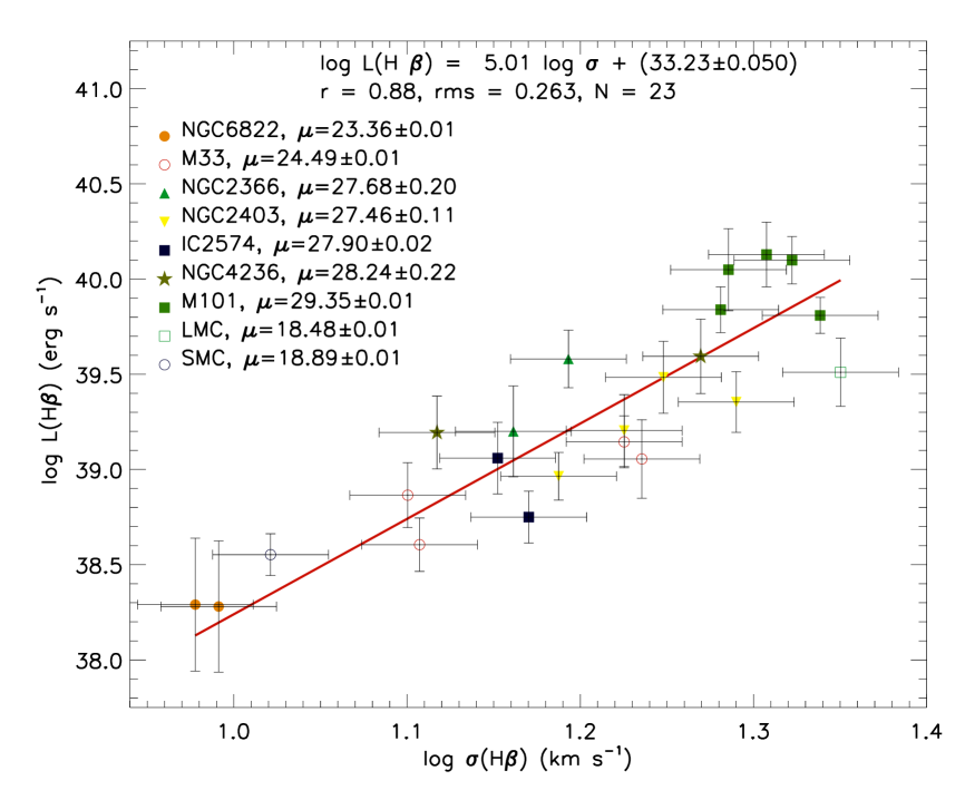
Figure 5.1: $L(\mathrm{H}\beta)-\sigma$ relation for the GEHR sample. The correlation parameters and the adopted individual distance moduli are given in the inset. The red line is the best fit for a fixed value of the slope.

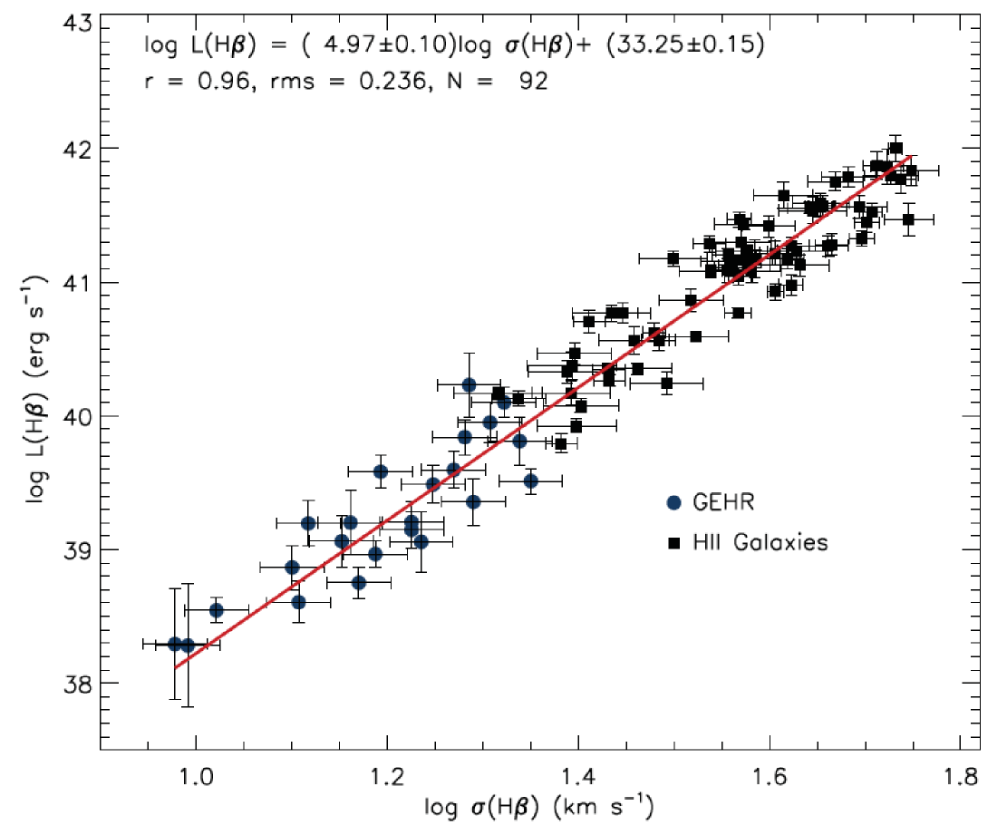
Figure 5.2: $L(\mathrm{H}\beta)-\sigma$ relation for the joint H ii galaxies and GEHR sample.

In detail, we first estimate the slope of the $L(\mathrm{H}\beta)-\sigma$ relation for H ii galaxies, using an arbitary value of $H_{0}$, since the slope is independent of $H_{0}$, to determine luminosities from the observed $\mathrm{H}\beta$ flux and the Hubble distance. We then determine the intercept of the relation from a fit to the ‘anchor’ GEHR sample, but fixing the slope to that determined in step one, i.e., that based on H ii galaxies.

Figure 5.1 shows the $L(\mathrm{H}\beta)-\sigma$ relation for the GEHR sample. The slope of the correlation has been fixed to the value obtained from the H ii galaxies sample fitting as explained above. The resulting GEHR sample $L(\mathrm{H}\beta)-\sigma$ correlation is:

$$\log L(\mathrm{H}\beta)=5.01\log\sigma+(33.23\pm 0.050)$$ (5.1)

with r.m.s. $\log L(\mathrm{H}\beta)=0.263$.

The $L(\mathrm{H}\beta)-\sigma$ correlation resulting from fitting jointly the H ii galaxies sample and the GEHR sample is shown in Figure 5.2 and is given by:

$$\log L(\mathrm{H}\beta)=(4.97\pm 0.10)\log\sigma+(33.25\pm 0.15)$$ (5.2)

with r.m.s. $\log L(\mathrm{H}\beta)=0.236$.

The final step of our procedure is to determine the value of $H_{0}$ by minimizing, over a grid of $H_{0}$ values, the function:

$$\chi^{2}(H_{0})=\sum\limits_{i=1}^{n}\frac{[L_{i}(\sigma_{i})-\tilde{L}_{i}(H_{0},f_{i},z_{i})]^{2}}{\sigma_{L,i}^{2}+\sigma_{\tilde{L},i}^{2}},$$ (5.3)

where the summation is over the H ii galaxies, $\sigma_{i}$ are the measured velocity dispersions, $L_{i}(\sigma)$ are the logarithmic luminosities estimated from the ‘distance indicator’ as defined in eq.(5.2), $\sigma_{L,i}$ are their errors propagated from the uncertainties in $\sigma$, the slope and intercept of the relation, $\tilde{L}_{i}(H_{o},f_{i},z_{i})$ are the logarithm of the luminosities obtained from the measured fluxes and redshifts by using a particular value of $H_{0}$ in the Hubble law to estimate distances, and $\sigma_{\tilde{L},i}$ are the errors in this last estimation of luminosities, propagated from the uncertainties in the fluxes and redshifts.

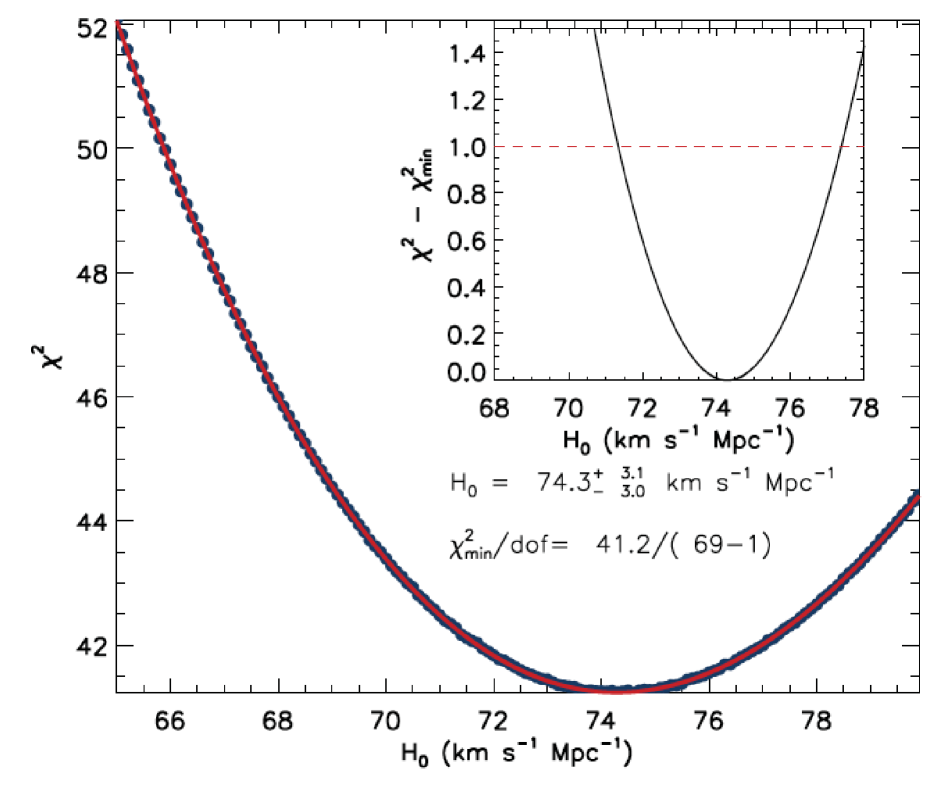
Figure 5.3: Values of $\chi^{2}$ for the grid of $H_{0}$. The solid line is a cubic fit to the points. The inset panel shows the value of $\chi^{2}-\chi^{2}_{min}$.

The value obtained for $H_{0}$ using the above described procedure is:

$$H_{0}=74.3^{+3.1}_{-3.0}\ \mathrm{Km\ s^{-1}\ Mpc^{-1}}\;.$$ (5.4)

Figure 5.3 shows the resulting $\chi^{2}$ for the grid of $H_{0}$ values used, with the solid line being a cubic fit to the points. The inset panel shows the value of $\chi^{2}-\chi^{2}_{min}$, from here we have obtained the $1\sigma$ confidence limits as the values of $H_{0}$ for which $\chi^{2}-\chi^{2}_{min}=1$ since the fit has only 1 degree of freedom (dof) .

Figure 5.4 shows the Hubble diagram for the sample of H ii galaxies used for the $H_{0}$ value determination. The continuous line shows the redshift run of the distance modulus, obtained from the linear Hubble law and the fitted $H_{0}$ value, whereas the points correspond to the individual H ii galaxy distance moduli obtained through the $L(\mathrm{H}\beta)-\sigma$ correlation.

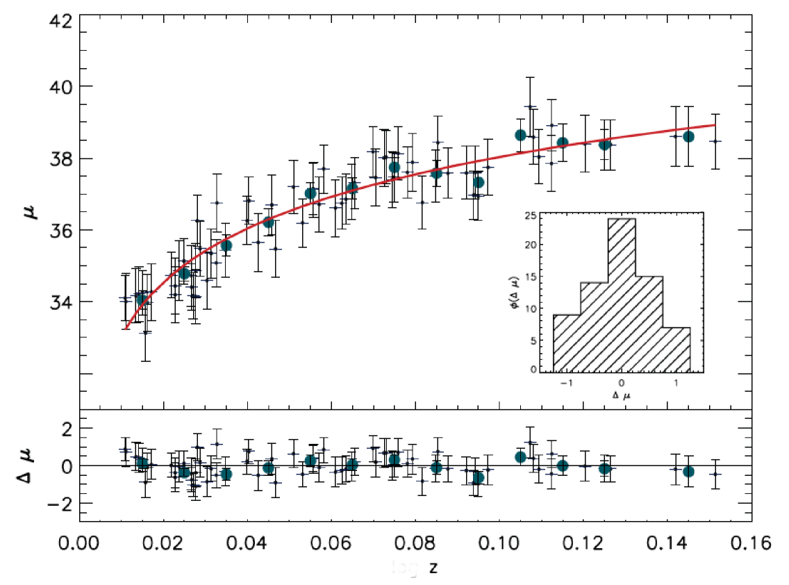
Figure 5.4: Hubble diagram for our sample of 69 H ii galaxies. The thick points are the mean values for bins of $0.01$ in redshift. The solid line shows the run with redshift of the distance modulus for $H_{0}=74.3$. Residuals are plotted in the bottom panel and their distribution is shown in the inset. The rms value is 0.57 mag.

5.2.1 Systematics

Table 5.2: Systematic Error Budget on the $H_{0}$ determination.

Symbol	Source	Error (km s-1 Mpc-1)
$\sigma_{a,b}$	Rotation,Multiplicity	0.7
$\sigma_{c}$	Stellar Winds	1.1
$\sigma_{d}$	Internal Extinction	0.7
$\sigma_{f}$	Object’s Age	1.4
$\sigma_{g}$	Malmquist Bias	2.1
$\sigma_{h}$	IMF	—-
Total		2.9

The most difficult problem when pursuing high precision cosmology is probably recognising and treating the systematic errors affecting the procedure. Here we will discuss the most important ones in the derivation of $H_{0}$ by means of the $L(\mathrm{H}\beta)-\sigma$ relation for giant bursts of star formation and HII galaxies. Table 5.2 shows the systematic error budget on the $H_{0}$ determination.

Malmquist bias

Malmquist bias is a selection effect affecting flux limited samples, consisting of the preferential detection of the most luminous objects as a function of distance and limiting flux. A flux limited sample is biased towards the bright end of the luminosity function because as the distance towards an object increases the limiting flux imposes a higher luminosity detection threshold.

The Malmquist bias for our flux limited sample was calculated following the procedure given by Giraud (1987). Basically the procedure consists in calculating the mean value for the absolute magnitudes distribution at every kinematic distance ($\langle M(\log D_{v})\rangle$) and compare it to the true mean value of the absolute magnitudes distribution ($M_{0}$); the resulting value is called $\Delta M(\log D_{v})$ and the bias is given by the expression:

$$b(\log D_{v})=\frac{\sigma_{0}^{2}}{\sigma_{M_{0}}^{2}+\sigma_{0}^{2}}\Delta M(\log D_{v}),$$ (5.5)

where, $D_{v}$ is given in $\mathrm{km\ s^{-1}}$, $\sigma_{0}$ is the true dispersion of residuals of the $L(\mathrm{H}\beta)-\sigma$ relation and $\sigma_{M_{0}}$ is the true dispersion of the distribution of absolute magnitudes of the sample. Finally the correction to $H_{0}$ at every kinematic distance is given by:

$$\Delta\log H=0.2b(\log D_{v}).$$ (5.6)

The main difference between our calculation and the one by Giraud (1987) is that whereas he used a gaussian distribution for the absolute magnitudes, we use a power law one.

Another consideration is that the true values for the absolute magnitude distribution parameters and the true dispersion of residuals for the $L(\mathrm{H}\beta)-\sigma$ relation are obviously not directly known, but since we have corrected the absolute magnitude distribution for selection bias using the $V_{max}$ method and using only the brighter end of the distribution for the parametric fit, we used directly the parameters obtained in section 4.4. On the other hand the true dispersion of residuals in the $L(\mathrm{H}\beta)-\sigma$ correlation can not be obtained, so we used instead the observed dispersion of residuals, hence our results are an upper limit to the true Malmquist bias.

Our main result is that the value of the Malmquist bias is quite small: $2.1\ \mathrm{km\ s^{-1}}$ at $z\sim 0.15$, and smaller at lower $z$.

Age

As discussed in §6.1.3, the value of $W(\mathrm{H}\beta)$ is a good indicator of the age of the starburst. Melnick, Terlevich & Terlevich (2000) have demonstrated that H ii galaxies with $W(\mathrm{H}\beta)<25\ \mathrm{\AA}$ do follow an $L(\mathrm{H}\beta)-\sigma$ relation with a similar slope but different intercept than the ones with larger $W(\mathrm{H}\beta)$. In principle we can conclude that age could be an important systematic effect present in the distances estimated from the $L(\mathrm{H}\beta)-\sigma$ relation.

For the study presented here, the starburst age is a controlled parameter in the sense that we have selected our sample to be composed of very young objects by putting a high lower limit to the value of $\mathrm{W}(\mathrm{H}\beta)>50\ \mathrm{\AA}$. Only the youngest bursts therefore were considered.

From the previous discussion it is clear that we expect to have only a small systematic effect from the evolution of the starburst on the determination of $H_{0}$; we have quantified it to be $\sim 1.4\ \mathrm{km\ s^{-1}\ Mpc^{-1}}$.

Chemical abundance

We have investigated the possible influence of chemical abundance over the $L(\mathrm{H}\beta)-\sigma$ relation but the results obtained are quite inconclusive. It appears that the abundance does not contribute decisively to the scatter in the relation and then its influence at least for our sample with small dynamic range is very small.

Radius

As we already discussed in chapter 4, the size of the objects definitely contribute as a parameter to explain the scatter in the $L(\mathrm{H}\beta)-\sigma$ relation but it appears that sizes as measured from SDSS DR7 data are severely overestimated, although probably systematically. Further investigation is therefore required to determinate the extent of its contribution as source of error. However, the uncertainties derived from not considering the size as a parameter are already considered, since the errors in the $L(\mathrm{H}\beta)-\sigma$ relation are propagated to the random error in the determination of $H_{0}$.

Extinction

We have already considered the effect of reddening and underlying absorption on the measurements. Yet, concerned about the Balmer decrement not allowing us to correct completely for internal extinction, we have estimated the corresponding systematic error in the $H_{0}$ determination.

Environment

In order to explore the possible effect of the environment in the $L(\mathrm{H}\beta)-\sigma$ correlation, we have studied the close environment ($\sim 200h^{-1}_{75}\ \mathrm{kpc}$) for the objects in our sample plus SDSS DR7 data. We used the available spectroscopic and photometric redshifts to explore the presence of close and possibly interacting companions to our target sample.

The complete description of the study and the results are presented in Koulouridis et al. (2013) where we conclude that the $L(\mathrm{H}\beta)-\sigma$ correlation is not affected by environmental or host galaxy differences of isolated and paired H ii galaxies.

5.3 Summary

It is indisputable that in the epoch of intense studies aimed at measuring the dark energy equation of state, it is of paramount importance to minimize the amount of priors needed to successfully complete such a task. One such prior is the Hubble constant $H_{0}$ and its measurement at the $\sim 1\%$ accuracy level has been identified as a necessary prerequisite for putting effective constraints on the dark energy, on neutrino physics and even on tests, at cosmological scales, of general relativity (see Suyu et al., 2012). Furthermore, it is highly desirable to have independent determinations of $H_{0}$, since this will help understand and control systematic effects that may affect individual methods and tracers of the Hubble expansion.

It is within this latter strategy that our current work falls. We have carried out VLT and Subaru observations of a sample of nearby H ii galaxies, identified in the SDSS DR7 catalogue and 2m class telescopes spectrophotometry, in order to define their $L(\mathrm{H}\beta)-\sigma$ correlation, which we use to estimate the value of the Hubble constant. This is achieved by estimating the zero-point of the distance indicator using giant H ii regions in nearby galaxies, for which accurate independent distance measurements exist (based on Cepheids, RR Lyrae, TRGB and eclipsing binaries).

Using our final and clean of systematic effects sample of 69 H ii galaxies with $z\raise-3.0pt\hbox{\hbox to0.0pt{\hbox{$\sim$}\hss}\raise 4.0pt\hbox{$<$}\ }0.16$, we obtain:
$H_{0}=74.3\pm 3.1$(random) $\pm 2.9$ (systematic) km s^-1 Mpc^-1,
independently confirming the recent SNae Ia-based results of Riess et al. (2011).

Chapter 6 The Dark Energy Equation of State

The true method of knowledge is experiment.

— W. Blake, All Religions are One (1788)

The nature of dark energy is one of the outstanding questions in modern cosmology. Its multiple connections with almost every aspect of physics makes the problem of understanding its inherent features a specially important one. As already said (see §2.3), many theoretical explanations have been advanced to explain the problem, but to date there is no convincing answer.

Dark energy can be explored in the first instance by means of constraining the value of its equation of state parameter, $w$, in general given as:

$$p_{Q}=w(z)\rho_{Q}\;,$$ (6.1)

where $p_{Q}$ is the pressure and $\rho_{Q}$ is the density of the postulated dark energy fluid; in the special case of $w=-1$ we are dealing with a cosmological constant.

Many of the proposed models can be parametrised by:

$$w(z)=w_{0}+w_{1}f(z)\;,$$ (6.2)

where $w_{0}=w(z=0)$ and $f(z)$ is a function of redshift. An example is the CPL model where $f(z)=z/(1+z)$ (Chevallier & Polarski, 2001; Linder, 2003; Peebles & Ratra, 2003; Dicus & Repko, 2004; Wang & Mukherjee, 2006).

We can constrain the value of $w$, as well as other cosmological parameters, using high-$z$ cosmological tracers as described in §3.3. In this Chapter we explore the use of H ii galaxies as cosmological tracers to high-$z$.

6.1 Observations and Data Reduction

A sample of 9 star forming galaxies with $EW(\mathrm{H}\beta)>50\ \mathrm{\AA}$ was selected from Hoyos et al. (2005); Erb et al. (2006a, b) and Matsuda et al. (2011). The redshift range covered was $0.64\leq z\leq 2.33$. The rationale for the selection criteria was the same as described in section §4.1.

The high spectral resolution spectroscopic observations were obtained using the X-Shooter echelle spectrograph (Vernet et al., 2011) at the Cassegrain focus of the ESO-VLT in Paranal, Chile. The observations were conducted during the nights of September 29th and 30th, 2013.

Xshooter is a three arm intermediate resolution echelle spectrograph. We obtained spectra for the three arms though in the end we only used the UVB and NIR arms data, the typical spectral resolution on the UVB arm was $\sim 10000$, whereas in the NIR arm was $\sim 8000$ with an $0.8\hbox{${}^{\prime\prime}$}$ slit.

The data reduction was carried out using the XShooter pipeline V2.3.0 over the GASGANO V2.4.3 environment using the ‘physical model mode’ reduction.

6.2 Data Analysis

6.2.1 Emission line widths

A gaussian fit was performed on the 1D spectra profiles of the $[\mathrm{O\ III}]\ \lambda 5007$Å  and $\mathrm{H}\alpha$ lines when available. These fits were performed using the IDL routine gaussfit. Figure 6.1 shows a typical fit to the $[\mathrm{O\ III}]\ \lambda 5007$Å line.

The 1$\sigma$ uncertainties of the FWHM were estimated using a Montecarlo analysis. A set of random realizations of every spectrum was generated using the data poissonian 1$\sigma$ 1-pixel uncertainty. Gaussian fitting for every synthetic spectrum in the set was performed afterwards, and we obtained a distribution of FWHM measurements from which the 1$\sigma$ uncertainty for the FWHM measured in the spectra follows.

Figure 6.1: Typical gaussian fit to an $[\mathrm{O\ III}]\ \lambda 5007$Å line. Upper panel: The single gaussian fit is shown with a dashed line (thick black). The parameters of the fits are shown in the top left corner. Lower panel: The residuals from the fit.

Table 6.1: FWHM of $[\mathrm{O\ III}]\ \lambda 5007$ and $\mathrm{H}\alpha$ from the XShooter high dispersion spectra.

(1)	(2)	(3)	(4)	(5)	(6)	(7)
Index	Name	$\mathbf{z_{hel}}$	$\mathbf{\lambda_{c}}$ ($\mathbf{[\mathrm{O\ III}]\ \lambda 5007}$)	FWHM($\mathbf{[\mathrm{O\ III}]\ \lambda 5007}$)	$\mathbf{\lambda_{c}}$ ($\mathbf{\mathrm{H}\alpha}$)	FWHM ($\mathbf{\mathrm{H}\alpha}$)
			(nm)	($\mathrm{km\ s^{-1}}$)	(nm)	($\mathrm{km\ s^{-1}}$)
401	HoyosD2 5	0.6364	819.359 $\pm$ 0.002	96.6 $\pm$ 1.3	1073.861 $\pm$ 0.012	113.3 $\pm$ 7.8
273	Q2343-BM133	1.4774	1240.440 $\pm$ 0.003	134.1 $\pm$ 1.5	1625.881 $\pm$ 0.005	142.6 $\pm$ 2.1
301	Q2343-BX660	2.1735	1589.181 $\pm$ 0.006	150.9 $\pm$ 2.5	2082.558 $\pm$ 0.012	—
404	HoyosD2 1	0.8510	926.740 $\pm$ 0.015	118.2 $\pm$ 11.4	—	—
287	Q2343-BX435	2.1119	1557.924 $\pm$ 0.034	171.3 $\pm$ 15.6	2042.258 $\pm$ 0.021	178.6 $\pm$ 7.2
285	Q2343-BX418	2.3052	1654.870 $\pm$ 0.002	135.3 $\pm$ 1.0	—	—
7	Q2343-BX436	2.3277	1666.438 $\pm$ 0.025	180.0 $\pm$ 10.8	—	—
8	MatsudaC3HAE3	2.2397	1622.102 $\pm$ 0.054	292.7 $\pm$ 23.4	—	—
9	HoyosD2 12	0.6800	841.988 $\pm$ 0.002	84.4 $\pm$ 1.2	—	—

Table LABEL:tab:tab601 lists the FWHM measurements for the high resolution observations prior to any correction such as instrumental or thermal broadening. Column (1) is an index number, column (2) is the name, column (3) is the heliocentric redshift, columns (4) and (5) are the measured $[\mathrm{O\ III}]\ \lambda 5007$ central wavelength in $\mathrm{nm}$ and FWHM in $\mathrm{km\ s^{-1}}$ whereas columns (6) and (7) are the $\mathrm{H}\alpha$ central wavelength in $\mathrm{nm}$ and FWHM in $\mathrm{km\ s^{-1}}$.

The observed velocity dispersions ($\sigma_{o}$) – and their 1$\sigma$ uncertainties – have been derived from the FWHM measurements of the $[\mathrm{O\ III}]\lambda 5007$ and $\mathrm{H}\alpha$ lines as:

$$\sigma_{o}\equiv\frac{FWHM}{2\sqrt{2\ ln(2)}}$$ (6.3)

Corrections for thermal ($\sigma_{th}$) and instrumental ($\sigma_{i}$) broadening have been applied. The corrected value is given by the expression:

$$\sigma=\sqrt{\sigma_{o}^{2}-\sigma_{th}^{2}-\sigma_{i}^{2}}$$ (6.4)

The 1$\sigma$ uncertainties for the velocity dispersion have been propagated from the $\sigma_{o}$ values.

The thermal broadening was calculated assuming a Maxwellian velocity distribution of the hydrogen and oxygen ions, from the expression:

$$\sigma_{th}\equiv\sqrt{\frac{kT_{e}}{m}},$$ (6.5)

where $k$ is the Boltzmann constant, $m$ is the mass of the ion in question and $T_{e}$ is the electron temperature in degrees Kelvin. $T_{e}$ has been assumed to have a value of $10000$ K.

In the cases where we do not have $\mathrm{H}\alpha$ velocity dispersions we have corrected the $[\mathrm{O\ III}]\lambda 5007$ velocity dispersion by the mean difference calculated from the cases where we have both values.

As discused previously (see chapter 4) imposing an upper limit to the velocity dispersion such as $\log\sigma($H$\beta)\lesssim 1.8$ $\mathrm{km\ s^{-1}}$, minimizes the probability of including rotationally supported systems and/or objects with multiple young ionising clusters contributing to the total flux and affecting the line profiles. Therefore from the sample we selected all objects having $\log\sigma(\mathrm{H}\alpha)<1.86$ $\mathrm{km\ s^{-1}}$ thus restricting the sample to 6 objects.

The corrected velocity dispersions for the $\mathrm{H}\alpha$ lines and their 1-$\sigma$ uncertainties are shown in Table LABEL:tab:tab602, in column (4).

6.2.2 Fluxes

In the case of objects taken from Matsuda et al. (2011) and Erb et al. (2006a, b), H$\alpha$ fluxes were obtained form the literature directly, then we can easily deduce from the reddened corrected $f(\mathrm{H}\alpha)$, the $f(\mathrm{H}\beta)$ values from the theoretical ratio between both. In the case of objects taken from Hoyos et al. (2005), luminosities have been derived using (see Terlevich & Melnick, 1981):

$$B_{C}=-2.5\log[L_{o}(\mathrm{H}\beta)/EW_{\lambda}]+79.4\ \;,$$ (6.6)

where $B_{C}$ is the absolute blue continuum magnitude, $L_{o}(\mathrm{H}\beta)$ is the $\mathrm{H}\beta$ luminosity and $EW_{\lambda}$ is the $\mathrm{H}\beta$ equivalent width. Table LABEL:tab:tab602, column (6) shows the adopted $\mathrm{H}\beta$ fluxes and their 1-$\sigma$ uncertainties.

Table 6.2: Adopted values for the $L-\sigma$ relation of high-$z$ H ii Galaxies.

(1)	(2)	(3)	(4)	(5)	(6)
Index	Name	$\mathbf{z_{hel}}$	$\mathbf{\log\sigma}$ ($\mathbf{\mathrm{H}\alpha}$)	$\mathbf{\log L}$ ($\mathbf{\mathrm{H}\beta}$)	$\mathbf{f}$ ($\mathbf{\mathrm{H}\beta}$)
			($\mathrm{km\ s^{-1}}$)	($\mathrm{erg\ s^{-1}}$)	($10^{-17}\ \mathrm{erg\ s^{-1}\ cm^{-2}}$)
6	HDF-BX1277	2.2713	1.799 $\pm$ 0.062	$41.812^{+0.038}_{-0.042}$	1.853 $\pm$ 0.070
10	HDF-BX1332	2.2136	1.732 $\pm$ 0.129	$41.704^{+0.044}_{-0.050}$	1.538 $\pm$ 0.105
17	HDF-BX1479	2.3745	1.663 $\pm$ 0.170	$41.532^{+0.048}_{-0.053}$	0.874 $\pm$ 0.070
22	Q0201-B13	2.1663	1.792 $\pm$ 0.070	$41.418^{+0.039}_{-0.043}$	0.839 $\pm$ 0.035
25	Q1623-BX214	2.4700	1.740 $\pm$ 0.110	$41.900^{+0.046}_{-0.052}$	1.853 $\pm$ 0.140
26	Q1623-BX215	2.1814	1.845 $\pm$ 0.093	$41.726^{+0.043}_{-0.048}$	1.678 $\pm$ 0.105
33	Q1623-BX429	2.0160	1.756 $\pm$ 0.168	$41.669^{+0.053}_{-0.060}$	1.783 $\pm$ 0.175
34	Q1623-BX432	2.1817	1.732 $\pm$ 0.121	$41.777^{+0.041}_{-0.046}$	1.888 $\pm$ 0.105
38	Q1623-BX453	2.1816	1.785 $\pm$ 0.028	$42.185^{+0.035}_{-0.038}$	4.825 $\pm$ 0.070
71	Q1700-MD154	2.6291	1.756 $\pm$ 0.259	$41.855^{+0.060}_{-0.069}$	1.434 $\pm$ 0.175
273	Q2343-BM133	1.4774	1.756 $\pm$ 0.007	$42.087^{+0.037}_{-0.040}$	10.035 $\pm$ 0.280
74	Q2343-BM181	1.4951	1.591 $\pm$ 0.189	$41.173^{+0.068}_{-0.080}$	1.189 $\pm$ 0.175
285	Q2343-BX418	2.3052	1.758 $\pm$ 0.004	$42.006^{+0.036}_{-0.040}$	2.797 $\pm$ 0.070
86	Q2343-BX429	2.1751	1.708 $\pm$ 0.136	$41.723^{+0.043}_{-0.048}$	1.678 $\pm$ 0.105
287	Q2343-BX435	2.1119	1.863 $\pm$ 0.019	$41.919^{+0.040}_{-0.044}$	2.832 $\pm$ 0.140
301	Q2343-BX660	2.1735	1.808 $\pm$ 0.008	$42.014^{+0.039}_{-0.043}$	3.287 $\pm$ 0.140
105	Q2346-BX120	2.2664	1.792 $\pm$ 0.084	$41.810^{+0.042}_{-0.046}$	1.853 $\pm$ 0.105
107	Q2346-BX244	1.6465	1.623 $\pm$ 0.279	$41.478^{+0.068}_{-0.081}$	1.888 $\pm$ 0.280
109	Q2346-BX405	2.0300	1.699 $\pm$ 0.035	$42.115^{+0.035}_{-0.038}$	4.895 $\pm$ 0.070
401	HoyosD2 5	0.6364	1.597 $\pm$ 0.008	$41.438^{+0.022}_{-0.023}$	17.960 $\pm$ 1.490
404	HoyosD2 1	0.8510	1.695 $\pm$ 0.045	$41.711^{+0.022}_{-0.023}$	16.525 $\pm$ 1.360

6.2.3 Data from literature

Since after applying the $\log\sigma(\mathrm{H}\alpha)<1.86$ $\mathrm{km\ s^{-1}}$ criterium we ended with a sample of only 6 objects, we decided to use also data from the literature. Following the same criterium, we selected a sample of 15 objects from Erb et al. (2006a, b) for which $\sigma(\mathrm{H}\alpha)$ and $f(\mathrm{H}\alpha)$ are given. Table LABEL:tab:tab602, columns (4) and (6) shows the adopted data from the Erb et al. (2006a, b) sample. In the same table, the objects with index larger that $200$ are our observed sample and we show their final adopted data.

6.3 Results and Discussion

Using the concordance $\Lambda$CDM cosmology as fiducial model we can calculate the luminosities for all the objects in our new sample and then construct the corresponding $L-\sigma$ correlation. The values of the luminosities calculated following this procedure are shown in Table LABEL:tab:tab602, column (5). Figure 6.2 shows the $L-\sigma$ relation for the high-z sample of H ii galaxies combined with the local sample (S3) from Figure 4.20. It is clear that there is a remarkable similarity between both.

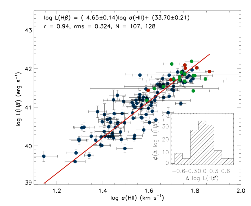
Figure 6.2: $L-\sigma$ relation for the combined local and high-z samples of H ii galaxies, the blue points are the local sample, the red points indicate our high-$z$ observations, and the green ones, the data from Erb et al. (2006a, b). The inset shows the distribution of the residuals of the fit.

Using the $L-\sigma$ relation for the ‘best sample’ that we used to estimate the value of $H_{0}$ given in eq. (5.2), we can calculate a value for $L(\mathrm{H}\beta)$ that can be compared with the value obtained from $f(\mathrm{H}\beta)$, $z$ and a cosmological model. In general we can minimise the function:

$$\chi^{2}(\mathbf{p})=\sum\limits_{i=1}^{n}\frac{[L_{i}(\sigma_{i})-\tilde{L}_{i}(\mathbf{p},f_{i},z_{i})]^{2}}{\sigma_{L,i}^{2}+\sigma_{\tilde{L},i}^{2}},$$ (6.7)

where the summation is over the combined sample of local and high-$z$ H ii galaxies, $\sigma_{i}$ are the measured velocity dispersions, $L_{i}(\sigma)$ are the logarithmic luminosities estimated from the ‘distance indicator’ as defined in equation (5.2), $\sigma_{L,i}$ are their errors propagated from the uncertainties in $\sigma$, the slope and intercept of the relation, $\tilde{L}_{i}(\mathbf{p},f_{i},z_{i})$ is the logarithm of the luminosities obtained from the measured fluxes and redshifts by using a particular set of cosmological parameters $\mathbf{p}$, and $\sigma_{\tilde{L},i}$ are the errors in this last estimation of luminosities, propagated from the uncertainties in the fluxes and redshifts.

The most general set of cosmological parameters, assuming a flat universe and an insignificant value of $\Omega_{r}$ and using the CPL model for parametrising the value of $w(z)$, is given by $\mathbf{p}=\{H_{0},\Omega_{m},w_{0},w_{1}\}$, in this case the value of the luminosity distance used to estimate the value of $\tilde{L}_{i}(\mathbf{p},f_{i},z_{i})$, is given by,

$$D_{L}=\frac{c(1+z)}{H_{0}}\int_{0}^{z}{\frac{dz^{\prime}}{\sqrt{\Omega_{m}(1+z^{\prime})^{3}+(1-\Omega_{m})(1+z^{\prime})^{3(1+w_{0}+w_{1})}\exp[-3w_{1}z^{\prime}/(z^{\prime}+1)]}}}\;.$$ (6.8)

In Figure 6.3 we show a Hubble diagram for the joint local and high-$z$ samples of H ii galaxies, together with the $\Lambda$-CDM model, a model without cosmological constant and a phantom energy model, all of them assuming the value of $H_{0}$ obtained in the previous chapter. From the figure it is clear that our data favors the concordance $\Lambda$-CDM model.

If we assume a cosmological constant and minimise for $\mathbf{p}=\{H_{0},\Omega_{m}\}$, using different combinations of our high-$z$ sample and our local ‘benchmark’ sample (S3) of 107 H ii galaxies, we obtain the results shown in Figure 6.4, we have used asymmetrical errors in the logarithm of luminosity following the procedure detailed in Barlow (2004) to weight the $\chi^{2}$ function:

$$\sigma_{\tilde{L},i}=\sigma_{1}+\sigma_{2}[\tilde{L}_{i}(\mathbf{p},f_{i},z_{i})-L_{i}(\sigma_{i})]\ ,$$ (6.9)

where $\sigma_{1}=2\sigma_{p}\sigma_{n}/(\sigma_{p}+\sigma_{n})$, $\sigma_{2}=(\sigma_{p}-\sigma_{n})/(\sigma_{p}+\sigma_{n})$ and $\sigma_{p}$ is the upper error whereas $\sigma_{n}$ is the lower one.

It is clear form Figure 6.4 that the solutions are not very restrictive for $\Omega_{m}$ but are in good accord with other determinations for $H_{0}$. It is also clear that when we use the full 21 high-$z$ sample instead of only the best 6 objects, there are obtained better restrictions in the $\{H_{0},\Omega_{m}\}$ plane, even when many of these objects have large errors in their measured values of $\sigma$.

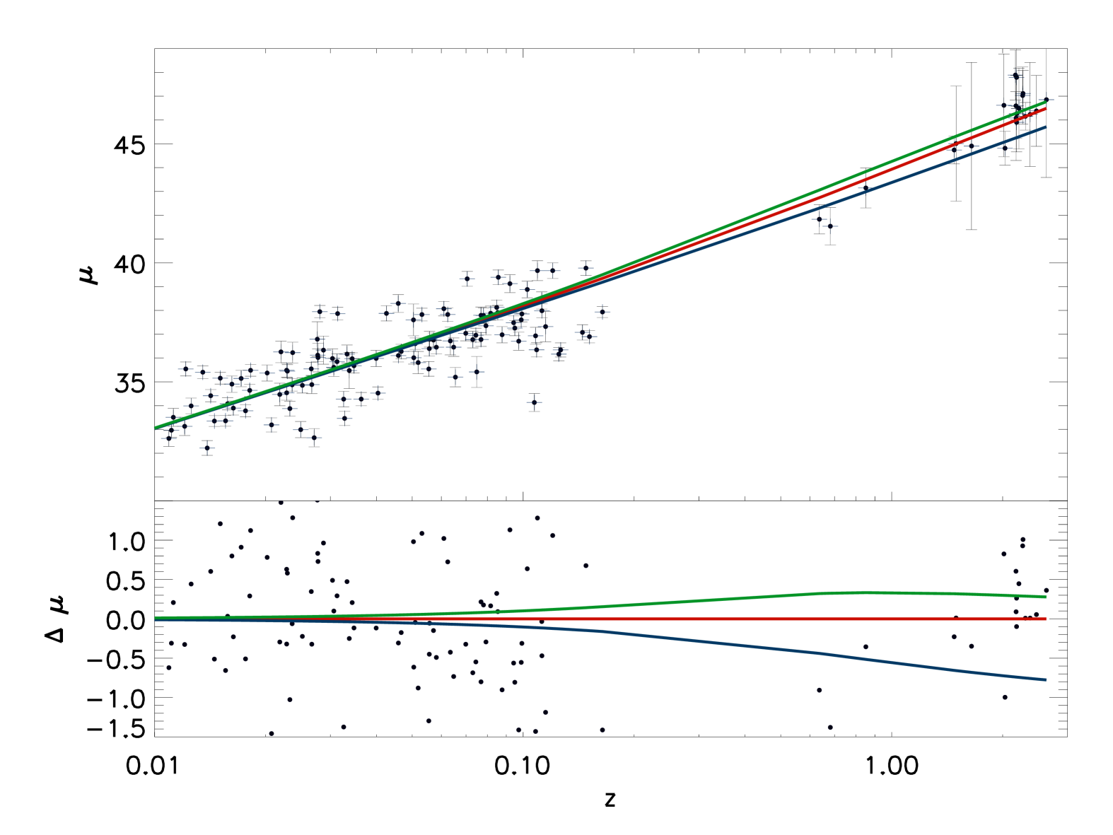
Figure 6.3: Upper panel: Hubble diagram for the joint local and high-z samples, the red line is the concordance $\Lambda$-CDM model, the green line is a model with $w_{0}=-2$ and $w_{1}=0.0$, the blue line is a model without cosmological constant. Lower panel: The Differential Hubble diagram showing the same data points and models.

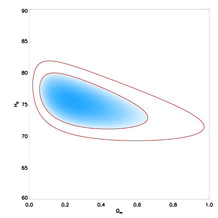
(a)

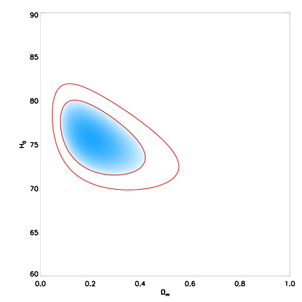
(b)

Figure 6.4: Solution spaces for $\mathbf{p}=\{H_{0},\Omega_{m}\}$. Panel (a) shows the solution space when we are using our observed sample of 6 high-$z$ H ii galaxies combined with the 107 local H ii galaxies from (S3). We are assuming a cosmological constant and using asymmetrical errors in the logarithm of luminosity. Panel (b) shows the same but using the combined 21 objects high-$z$ sample and the local (S3) sample, also using asymmetrical errors. In both panels we show the 1 and 2-$\sigma$ contours.

Assuming the value of $H_{0}$ obtained in the previous chapter, $w_{1}=0$ and again using different combinations of high-$z$ and local H ii  galaxies samples, we obtain the results shown in Figure 6.5 for $\mathbf{p}=\{\Omega_{m},w_{0}\}$, again we have used asymmetrical errors in the logarithm of luminosity as explained above. From the figure it is clear that we have obtained only weak restrictions in the $\{\Omega_{m},w_{0}\}$ plane, but we must remember that we are using only 21 high-$z$ objects and that we can combine the obtained results with other determinations e.g. SNe Ia results.

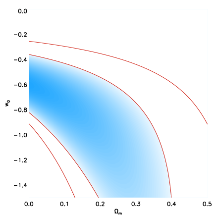
(a)

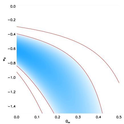
(b)

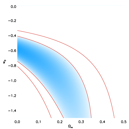
(c)

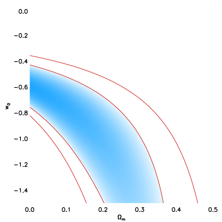
(d)

Figure 6.5: Solution spaces for $\mathbf{p}=\{\Omega_{m},w_{0}\}$. Panel (a) shows the solution space when we are using our observed sample of 6 high-$z$ H ii galaxies and are assuming a cosmological constant and asymmetrical errors in the logarithm of luminosity. Panel (b) shows the same but joining the 6 high-$z$ objects with the local sample (S3) of 107 objects. Panel (c) shows the same solution space but using the combined 21 objects high-$z$ sample. Panel (d) is as (c) but joining the high-$z$ sample with the local (S3) sample. In all panels we show the 1 and 2-$\sigma$ contours.

Following the same procedure, assuming the concordance value for $\Omega_{m}$, and using combinations of our high-$z$ and local H ii galaxies samples, we analyze the restrictions in the plane $\mathbf{p}=\{w_{0},w_{1}\}$, the results are shown in Figure 6.6, together with the line $w_{0}=w_{1}$, points above this line violate early matter domination and are disfavoured by the data. From the figure, it is clear that we need a larger sample for obtaining meaningful restrictions on this plane, the obtained restrictions are extremely weak.

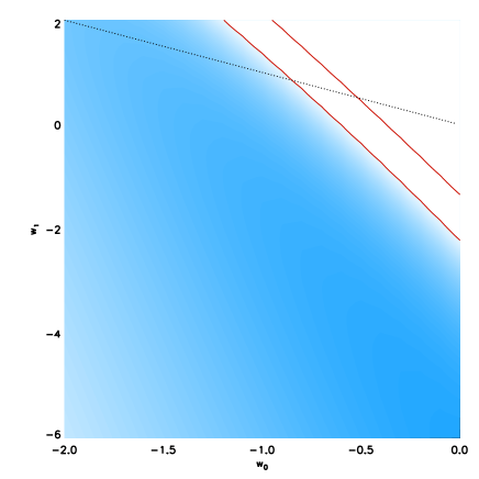
(a)

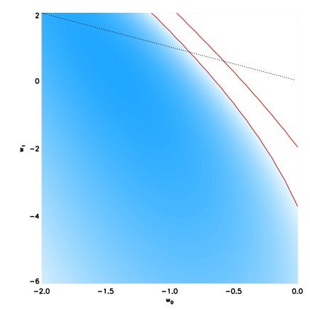
(b)

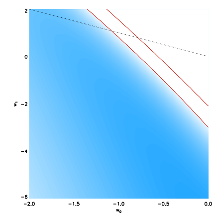
(c)

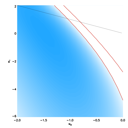
(d)

Figure 6.6: Solution spaces for $\mathbf{p}=\{w_{0},w_{1}\}$. Panel (a) shows the solution space where we are using our observed sample of 6 high-$z$ H ii galaxies and are assuming a cosmological constant and asymmetrical errors in the logarithm of luminosity. Panel (b) shows the same but joining with the local sample (S3). Panel (c) shows the same solution space but using the combined 21 objects high-$z$ sample and asymmetrical errors. Panel (d) is as (c) but joining with the local (S3) sample. In all panels we show the 1 and 2-$\sigma$ contours and the line $w_{0}=w_{1}$.

In Figure 6.7, we compare our results for the space $\mathbf{p}=\{\Omega_{m},w_{0}\}$ with recent results from SNe Ia, CMB and BAO. Form the figure it is clear that our results are weaker than the ones for SNe Ia, but this is not surprising since in our case we have only 128 objects vs 580 SNe Ia, altough we must remember that we have 17 high-$z$ objects ($z>1.5$) whereas the maximum redshift for SNe Ia is $\sim 1.5$.

In Figure 6.8, we compare our results for the space $\mathbf{p}=\{w_{0},w_{1}\}$ with recent combined results from SNe Ia, CMB and BAO. Form the figure it is clear that our results are much weaker that the combined ones for the other methods, but we must consider that we are comparing results form only one method versus the combined from several ones. In the other hand, one compelling result is that most of our solution space is below the region $w_{0}+w_{1}>0$, and then is compatible with other results.

(a)

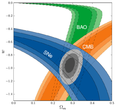
(b)

Figure 6.7: Comparison on restrictions of the plane $\mathbf{p}=\{\Omega_{m},w_{0}\}$. Panel (a) shows our results, obtained as described in the text for the combined high-$z$ sample of 21 H ii galaxies and local (S3) sample, we show the 1 and 2-$\sigma$ contours (random). Panel (b) results for SNe Ia, CMB and BAOs, the 1, 2 and 3-$\sigma$ contours are shown (random plus systematic). Taken from Suzuki et al. (2012).

(a)

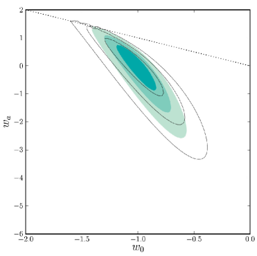
(b)

Figure 6.8: Comparison on restrictions of the plane $\mathbf{p}=\{\Omega_{m},w_{0}\}$. Panel (a) shows our results as described in the text for the combined high-$z$ sample of 21 H ii galaxies and local (S3) sample, we show the 1 and 2-$\sigma$ contours (random). Panel (b) shows the same plane but with recent combined results from SNe Ia, CMB, BAOs, and $H_{0}$; the 1, 2 and 3-$\sigma$ contours are shown both with (solid contours) and without (shaded contours) systematic errors. Points above the dotted line ($w_{0}+w_{a}>0$) violate early matter domination and are disfavoured by the data. Taken from Suzuki et al. (2012).

In general the obtained results are in line with other recent determinations, the general weakness of our determination can be attributed to the small number of intermediate to high-$z$ data (only 21 objects), of which only 6 have high quality observations, whereas the other 15 objects are taken from the literature, and have observations conducted with other purposes in mind and hence are of lower quality for our requirements.

As discussed in Plionis et al. (2011) (and references therein), we can estimate the number of high-$z$ tracers required to reduce by a certain factor the cosmological parameters solution space using the figure of merit (FoM), defined as the reciprocal area of the $2\sigma$ contour in the parameter space of any two degenerate cosmological parameters. In this way a larger FoM indicates better restrictions to the cosmological parameters. Plionis et al. (2011) use the parameter $S$ or ‘reduction factor’ to compare the ratio of FoM of SNe Ia + high-$z$ tracers to that of only SNe Ia. They found that the number of high-$z$ tracers needed to obtain a given S in the QDE model ( in which $w_{1}=0$ but $w_{0}$ changes in time) and when combined with the intermediate and low-$z$ SNa Ia, can be expressed as:

$$N_{Hz}\simeq 187S/S_{100}-88\,$$ (6.10)

where $S_{100}=1.87\log(\left<\sigma_{\mu}\right>^{-1}+0.74)+1.28$, and $\left<\sigma_{\mu}\right>$ is the mean distance modulus error for the tracer. In the case of H ii galaxies, ${\sigma_{\mu}}\simeq 0.6$, then $S_{100}\simeq 1.99$ and consequently in order to obtain a reduction to $2$ in $S$, we need around 100 high-$z$ H ii galaxies. We can visualize that in Figure 6.7 panel (b) for the $\{w_{0},w_{1}\}$ plane, where a factor 2 reduction means that $2\sigma$ contours would be similar to the actual $1\sigma$ SNe Ia contours. For the case of the CPL model, where $w_{1}$ is variable then the same result can be expressed as:

$$N_{Hz}\simeq 404S/S_{100}-300\,$$ (6.11)

where $S_{100}=0.49\log(\left<\sigma_{\mu}\right>^{-1}+0.65)+1.09$. In the case of H ii galaxies $S_{100}\simeq 1.27$ and consequently in order to obtain a reduction of 2 in $S$, we need around 340 high-$z$ H ii galaxies.

As already said, a substantial improvement to the restrictions of cosmological parameters can be obtained combining a few hundreds of H ii galaxies with the existing SNe Ia data. The observation of this few hundreds of objects, is technically not so difficult, given the relative abundance of H ii galaxies, many of them appear in the field of view of many of the currently operational medium spectral resolution integrated field spectrographs (IFUs) in 8 m class telescopes, e.g. using KMOS at VLT we would require only a few nights of observation to obtain the required data.

6.4 Summary

We have used a sample of 6 H ii galaxies that were observed using the XShooter medium spectral resolution spectrograph at the ESO-VLT, in a redshift range of $0.6\leq z\leq 2.3$ combined with a sample of 15 H ii galaxies taken from the literature and our sample of 121 local H iigalaxies to obtain constraints on the $\{H_{0},\Omega_{m}\}$, $\{\Omega_{m},w_{0}\}$ and$\{w_{0},w_{1}\}$ planes.

The obtained constraints are, in general, in line with other determinations, although weaker. The weakness of our results can be attributed to the small size of the intermediate to high-$z$ sample, and the considerable size of the uncertainties in the data taken from the literature.

The best way to obtain better constraints on the diverse cosmological parameters would be to obtain medium spectral resolution data for a sample of a few hundreds of objects and combine them with the local H ii galaxies and SNe Ia data.

Chapter 7 General Conclusions

We are such stuff
As dreams are made on; and our little life
Is rounded with a sleep.

— William Shakespeare, The Tempest (1611), IV, i

We have established a workable methodology to exploit H ii galaxies as cosmic tracers through their $L(\mathrm{H}\beta)-\sigma$ relation. Using them as tracers, we have obtained constraints in the value of $H_{0}$ and in the $\{H_{0},\Omega_{m}\}$, $\{\Omega_{m},w_{0}\}$ and$\{w_{0},w_{1}\}$ spaces. The obtained constraints are in line with the results obtained to date from other methodologies.

The relationship between the integrated H$\beta$ line luminosity and the velocity dispersion of the ionised gas of H ii galaxies and giant extragalactic H ii regions has been known for some time (Terlevich & Melnick, 1981; Melnick et al., 1987). It represents an extremely interesting standard candle that, in principle, can be used up to $z\sim 4$ (Plionis et al., 2011). Locally we have used the H ii galaxies $L(\mathrm{H}\beta)-\sigma$ relation to obtain high precision measurements of the local Hubble parameter and at intermediate and high redshift to constrain the dark energy equation of state parameters space. The use of the H ii galaxies $L(\mathrm{H}\beta)-\sigma$  relation as a cosmic tracer has been recognised as a potential research case in the E-ELT MOS white paper (Evans et al., 2013).

The cosmic acceleration problem is one of the most important open issues in the whole of physics. Its solution could shed light over many other important problems in physics and astronomy. The observational evidence for the cosmic acceleration is strong and originates in many distinct probes. All the current probes are limited by systematic errors, that in many cases require a better comprehension.

The physical mechanism responsible for the cosmic acceleration is unclear. The current evidence is consistent with a cosmological constant but without ruling out dark energy theories or some other dynamical models.

Large observational efforts are necessary in order to better constrain the dark energy equation of state parameters. In Plionis et al. (2011), we show that to use a sample of high redshift probes is the best strategy to obtain better constraints in the parameters of the dark energy equation of state.

We have proposed the use of H ii galaxies $L(\mathrm{H}\beta)-\sigma$ relation, to determine the Hubble function to intermediate and high redshifts and to obtain stringent constraints for the dark energy equation of state. We have shown that a good determination of the zero point of the $L(\mathrm{H}\beta)-\sigma$ relation are necessary; in addition we must take care of all possible systematics that could affect this correlation, in order to succeed in our aims.

In Chávez et al. (2014), with a sample of 107 H ii galaxies, we find that the $L(\mathrm{H}\beta)-\sigma$ relation is stable to changes in the sample definition. Additionally, we tested the behaviour or the $L(\mathrm{H}\beta)-\sigma$ relation when additional parameters are considered, our results point clearly to the existence of a Fundamental Plane in H ii galaxies suggesting that the main mechanism of line broadening is linked to the gravitational potential of the young massive cluster, although affected by age and metallicity. In Koulouridis et al. (2013) we find that the $L(\mathrm{H}\beta)-\sigma$ relation is independent of the H ii galaxies environment.

In Chávez et al. (2012) we used a sample of 69 H ii galaxies ($z<0.16$), observed with high dispersion spectroscopy at Subaru-HDS and the VLT-UVES, and low dispersion spectrophotometry at 2m class telescopes, together with a local calibration of the $L(\mathrm{H}\beta)-\sigma$ relation based on 23 GEHR in 9 nearby galaxies, whose distances are known from primary distance indicators, as an alternative ‘geometric’ approach for estimating the Hubble constant. We obtained $H_{0}=74.3\pm 3.1$ (random) $\pm 2.9$ (systematic) $\mathrm{km\ s^{-1}\ Mpc^{-1}}$, in excellent agreement with, and independently confirming, the most recent SNe Ia-based results (Riess et al., 2011; Freedman et al., 2012). It is important to note that by using mutually independent methods for the $H_{0}$ determination, it is possible to achieve a better comprehension of the systematic uncertainties’ effects over every one of those methods, hence the importance of having alternative determinations of the Hubble constant.

We have applied the H ii galaxies $L(\mathrm{H}\beta)-\sigma$ relation as a cosmological probe at $0.6<z<3$. We have used a sample, selected from emission line galaxies surveys Hoyos et al. (e.g. 2005); Erb et al. (e.g. 2006b); Matsuda et al. (e.g. 2011), of 6 objects observed using X-Shooter at VLT combined with a sample of 15 objects taken from the literature to obtain constraints in the $\{H_{0},\Omega_{m}\}$, $\{\Omega_{m},w_{0}\}$ and$\{w_{0},w_{1}\}$ planes. The obtained constraints are in line with other determinations although weaker but we have shown that using a larger sample at high-$z$ we will be able to put much more stringent constraint on the dark energy equation of state parameters.

7.1 Future Work

The work to be done can be thought basically in terms of two partial objectives that must be accomplished:

1. To improve the $L(\mathrm{H}\beta)-\sigma$ relation zero point through new high quality observations of GEHR.

2. To obtain a large sample (about 300) of high quality velocity dispersion and flux data for high-$z$ H ii galaxies and using the improved $L(\mathrm{H}\beta)-\sigma$ relation zero-point to construct a better H ii galaxies Hubble diagram to high-$z$.

Having accomplished the above two objectives, we will use the Hubble diagram of H ii galaxies (possibly combined with SNe Ia data) to put stringent constraints to the dark energy equation of state (i.e. the expansion history of the Universe).

7.2 Improving the $L(\mathrm{H}\beta)-\sigma$ Relation Zero Point

In Chávez et al. (2012) the zero-point value, provided by the local calibrator of the GEHRs, represents the weak link towards a more accurate value of $H_{0}$ from the $L(\mathrm{H}\beta)-\sigma$ relation. This is due to the fact that for the local GEHRs, the high-dispersion spectroscopic data, that provided the $\sigma$ measurements, and the spectrophotometry, that provided the $L(\rm{H}\beta)$ values, date back mostly to the 1980’s, and better measurements can be carried out with modern instrumentation.

In order to improve the $L(\mathrm{H}\beta)-\sigma$ relation zero point we will need accurate integrated flux and high spectral resolution velocity dispersion measurements for a local GEHR sample.

We have assembled a sample of $\sim 50$ GEHRs in $\sim 20$ galaxies having accurate Cepheid distances for which we have measured their integrated $\mathrm{H}\beta$ fluxes at OAN-SPM and OAGH-Cananea. We are now measuring the $\sigma$ of their nebular emission lines from high-dispersion spectroscopy using CanHiS at OAGH and MEzCal at OAN. This larger sample, observed with modern instrumentation, will lead to a factor of two reduction in the uncertainty in the $H_{0}$ value measured via the L(H${}_{Balmer})-\sigma$ relation. It is important to note that our sample includes three GEHRs in NGC 4258, the so called ‘maser galaxy’ for which very precise ‘geometric’ distance measurements are available.

7.3 Cosmological Constraints from H ii Galaxies

The second main task to do, is to select a large sample of H ii  galaxies to intermediate and high-$z$ from emission line sources catalogs. This large sample will be observed using middle resolution spectrographs at 8 m class telescopes.

There are many emission line galaxies catalogs already published (e.g. Erb et al., 2006b, a; Kakazu, Cowie & Hu, 2007; Matsuda et al., 2011; Hoyos et al., 2005; Atek et al., 2010), from which we can select the candidates to be observed. The selection criteria will be roughly the same as those described in section 4.1.

In oder to observe the selected sample, one of the best options is to use IFUs, at large telescopes, e.g. VLT-KMOS. The reason for this is that several objects in the same field can be observed simultaneously, thus increasing notably the observation efficiency, and in this way exploiting one of the main advantages of H ii galaxies over other e.g. SNe Ia, i.e. their relatively high number density.

Appendix A Cosmological Field Equations

The purpose of this appendix is to derive the Cosmological Field Equations from the General Relativity (GR) Field Equations; the approach followed for the derivation is variational since this method is intuitive, easy to follow and, not the least, very powerful.

A.1 The General Relativity Field Equations

The GR Field Equations can be written as

$$R_{\mu\nu}-\frac{1}{2}g_{\mu\nu}R+\Lambda g_{\mu\nu}=-\kappa T_{\mu\nu},$$ (A.1)

or alternatively as

$$R_{\mu\nu}=-\kappa\left(T_{\mu\nu}-\frac{1}{2}Tg_{\mu\nu}\right)+\Lambda g_{\mu\nu},$$ (A.2)

where $R_{\mu\nu}$ is the Ricci Tensor, $T_{\mu\nu}$ is the Energy-Momentum Tensor, $g_{\mu\nu}$ is the Metric Tensor, $\Lambda$ is the cosmological constant and $\kappa$ is a constant given by

$$\kappa=8\pi G,$$ (A.3)

note that we are using units in which $c=1$.

Our general approach to obtain the GR field equations for the FRW metric will be simply to obtain variationaly the Ricci Tensor and then to use the value of the Energy-Momentum Tensor for a perfect fluid to obtain the right-hand side of the GR field equations.

A.2 The Euler-Lagrange Equations

From the calculus of variations we know that if we want to find a function that makes an integral dependent on that function stationary, on a certain interval, we can proceed as follows; first we have the integral that we want to make stationary

$$S=\int_{a}^{b}{L(q^{a},\dot{q}^{a},t)dt},$$ (A.4)

where we define $S$ as the action, $L$ is the Lagrangian which is dependent on $q^{a}$, a set of generalized coordinates ($a$ is an index running over all the elements of the set), $\dot{q}^{a}$, the set of the generalized coordinates time derivatives, $\dot{q}^{a}\equiv dq^{a}/dt$ and $t$, the time, a parameter.

The variation of the action can be written as

$$\delta S = \int_{a}^{b}{\left(\frac{\partial L}{\partial q^{a}}\delta q^{a}+\frac{\partial L}{\partial\dot{q}^{a}}\delta\dot{q}^{a}\right)dt}$$ (A.5)

$$= \int_{a}^{b}{\frac{\partial L}{\partial q^{a}}\delta q^{a}dt}+\int_{a}^{b}{\frac{\partial L}{\partial\dot{q}^{a}}\delta\dot{q}^{a}dt},$$ (A.6)

integrating the last term by parts and requiring the variation $\delta S$ to be zero (the condition for $S$ to be stationary), we have

$$\int_{a}^{b}{\frac{\partial L}{\partial q^{a}}\delta q^{a}dt}+\left[\frac{\partial L}{\partial\dot{q}^{a}}\delta q^{a}\right]_{a}^{b}-\int_{a}^{b}{\frac{d}{dt}\left(\frac{\partial L}{\partial\dot{q}^{a}}\right)\delta q^{a}dt} = 0$$ (A.7)

$$\left[\frac{\partial L}{\partial\dot{q}^{a}}\delta q^{a}\right]_{a}^{b}+\int_{a}^{b}{\left[\frac{\partial L}{\partial q^{a}}-\frac{d}{dt}\left(\frac{\partial L}{\partial\dot{q}^{a}}\right)\right]\delta q^{a}dt} = 0,$$ (A.8)

since $a$ and $b$ are fixed then the first term vanishes and in order for the integral to be zero, since $\delta q^{a}$ is arbitrary, then

$$\frac{d}{dt}\left(\frac{\partial L}{\partial\dot{q}^{a}}\right)-\frac{\partial L}{\partial q^{a}}=0$$ (A.9)

These are the Euler-Lagrange equations that must be satisfied in order to make the action stationary.

A.3 Variational Method for Geodesics

In order to obtain the equations for the geodesics, and from them read out the metric connection coefficients, we must solve the Euler-Lagrange equations for the Lagrangian

$$L=\frac{1}{2}g_{ab}\dot{x}^{a}\dot{x}^{b},$$ (A.10)

where $g_{ab}$ are the metric elements and $\dot{x}^{a}$ are the coordinates time derivatives. Applying the Euler-Lagrange equations over the Lagrangian we obtain

$$\frac{d}{dt}(g_{ac}\dot{x}^{a})-\frac{1}{2}(\partial_{c}g_{ab})\dot{x}^{a}\dot{x}^{b}=0$$ (A.11)

$$\dot{g}_{ac}\dot{x}^{a}+g_{ac}\ddot{x}^{a}-\frac{1}{2}(\partial_{c}g_{ab})\dot{x}^{a}\dot{x}^{b}=0$$ (A.12)

$$(\partial_{b}g_{ac})\dot{x}^{a}\dot{x}^{b}+g_{ac}\ddot{x}^{a}-\frac{1}{2}(\partial_{c}g_{ab})\dot{x}^{a}\dot{x}^{b}=0$$ (A.13)

$$g_{ac}\ddot{x}^{a}+(\partial_{b}g_{ac})\dot{x}^{a}\dot{x}^{b}-\frac{1}{2}(\partial_{c}g_{ab})\dot{x}^{a}\dot{x}^{b}=0,$$ (A.14)

since $\dot{x}^{a}$ and $\dot{x}^{b}$ commutes, then we have

$$g_{ac}\ddot{x}^{a}+\frac{1}{2}(\partial_{b}g_{ac}+\partial_{a}g_{bc}-\partial_{c}g_{ab})\dot{x}^{a}\dot{x}^{b}=0$$ (A.15)

$$g^{dc}[\ddot{x}^{a}+\frac{1}{2}(\partial_{b}g_{ac}+\partial_{a}g_{bc}-\partial_{c}g_{ab})\dot{x}^{a}\dot{x}^{b}]=0$$ (A.16)

$$\ddot{x}^{d}+\frac{1}{2}g^{dc}(\partial_{b}g_{ac}+\partial_{a}g_{bc}-\partial_{c}g_{ab})\dot{x}^{a}\dot{x}^{b}=0$$ (A.17)

$$\ddot{x}^{d}+\Gamma^{d}_{ab}\dot{x}^{a}\dot{x}^{b}=0$$ (A.18)

$$\ddot{x}^{a}+\Gamma^{a}_{bc}\dot{x}^{b}\dot{x}^{c}=0,$$ (A.19)

where $\Gamma^{a}_{bc}$ are the metric connection coefficients and were clearly defined as

$$\Gamma^{a}_{bc}=\frac{1}{2}g^{dc}(\partial_{b}g_{ac}+\partial_{a}g_{bc}-\partial_{c}g_{ab})$$ (A.20)

and from (A.17) we can read without effort the metric connection coefficients.

A.4 Application to the FRW Metric

Using the FRW metric a distance element can be written as

$$ds^{2}=dt^{2}-a^{2}(t)\left[\frac{dr^{2}}{1-kr^{2}}+r^{2}(d\theta^{2}+\sin^{2}\theta d\phi^{2})\right]$$ (A.21)

then the metric is given by

$$[g_{ab}]=\left(\begin{array}[]{cccc}1&0&0&0\\ 0&-\frac{a^{2}(t)}{1-kr^{2}}&0&0\\ 0&0&-a^{2}(t)r^{2}&0\\ 0&0&0&-a^{2}(t)r^{2}\sin^{2}\theta\\ \end{array}\right).$$ (A.22)

From the previous section, equation (A.14) is the easiest to use; then we will apply this equation successively for values of the index $c$ running from $0$ to $3$. In the case in which $c=0$ we have

$$g_{00}\ddot{x}^{0}-\frac{1}{2}[(\partial_{0}g_{11})\dot{x}^{1}\dot{x}^{1}+(\partial_{0}g_{22})\dot{x}^{2}\dot{x}^{2}+(\partial_{0}g_{33})\dot{x}^{3}\dot{x}^{3}]=0,$$ (A.23)

then substituting and solving we obtain

$$\ddot{t}+\frac{a\dot{a}}{1-kr^{2}}(\dot{r})^{2}+a\dot{a}r^{2}(\dot{\theta})^{2}+a\dot{a}r^{2}\sin^{2}{\theta}(\dot{\phi})^{2}=0,$$ (A.24)

from here we can read the metric connection coefficients

$$\Gamma^{0}_{11} = \frac{a\dot{a}}{1-kr^{2}}$$ (A.25)

$$\Gamma^{0}_{22} = a\dot{a}r^{2}$$ (A.26)

$$\Gamma^{0}_{33} = a\dot{a}r^{2}\sin^{2}{\theta}.$$ (A.27)

For the case when $c=1$ we have

$$g_{11}\ddot{x}^{1}+(\partial_{0}g_{11})\dot{x}^{1}\dot{x}^{0}+(\partial_{1}g_{11})\dot{x}^{1}\dot{x}^{1}-\frac{1}{2}[(\partial_{1}g_{11})\dot{x}^{1}\dot{x}^{1}+(\partial_{1}g_{22})\dot{x}^{2}\dot{x}^{2}+(\partial_{1}g_{33})\dot{x}^{3}\dot{x}^{3}]=0,$$ (A.28)

then substituting and solving we obtain

$$\ddot{r}+2\frac{\dot{a}}{a}\dot{t}\dot{r}+\frac{kr}{1-kr^{2}}(\dot{r})^{2}-r(1-kr^{2})(\dot{\theta})^{2}-r(1-kr^{2})\sin^{2}{\theta}(\dot{\phi})^{2}=0,$$ (A.29)

from here we can read the metric connection coefficients

$$\Gamma^{1}_{01} = \frac{\dot{a}}{a}$$ (A.30)

$$\Gamma^{1}_{11} = \frac{kr}{1-kr^{2}}$$ (A.31)

$$\Gamma^{1}_{22} = -r(1-kr^{2})$$ (A.32)

$$\Gamma^{1}_{33} = -r(1-kr^{2})\sin^{2}{\theta}.$$ (A.33)

For the case when $c=2$ we have

$$g_{22}\ddot{x}^{2}+(\partial_{0}g_{22})\dot{x}^{2}\dot{x}^{0}+(\partial_{1}g_{22})\dot{x}^{2}\dot{x}^{1}-\frac{1}{2}(\partial_{2}g_{33})\dot{x}^{3}\dot{x}^{3}=0,$$ (A.34)

then substituting and solving we obtain

$$\ddot{\theta}+2\frac{\dot{a}}{a}\dot{\theta}\dot{t}+2\frac{1}{r}\dot{\theta}\dot{r}-\sin{\theta}\cos{\theta}(\dot{\phi})^{2}=0,$$ (A.35)

from here we can read the metric connection coefficients

$$\Gamma^{2}_{02} = \frac{\dot{a}}{a}$$ (A.36)

$$\Gamma^{2}_{12} = \frac{1}{r}$$ (A.37)

$$\Gamma^{2}_{33} = -\sin{\theta}\cos{\theta}.$$ (A.38)

For the case when $c=3$ we have

$$g_{33}\ddot{x}^{3}+(\partial_{0}g_{33})\dot{x}^{3}\dot{x}^{0}+(\partial_{1}g_{33})\dot{x}^{3}\dot{x}^{1}+(\partial_{2}g_{33})\dot{x}^{3}\dot{x}^{2}=0,$$ (A.39)

then substituting and solving we obtain

$$\ddot{\phi}+2\frac{\dot{a}}{a}\dot{\phi}\dot{t}+2\frac{1}{r}\dot{\phi}\dot{r}+2\frac{\cos{\theta}}{\sin{\theta}}\dot{\phi}\dot{\theta}=0,$$ (A.40)

from here we can read the metric connection coefficients

$$\Gamma^{3}_{03} = \frac{\dot{a}}{a}$$ (A.41)

$$\Gamma^{3}_{12} = \frac{1}{r}$$ (A.42)

$$\Gamma^{3}_{23} = \frac{\cos{\theta}}{\sin{\theta}}=\cot{\theta}.$$ (A.43)

A.5 Obtaining the Ricci Tensor

Having the metric connection coefficients, the next step is to obtain the independent values of the Ricci tensor which is given by

$$R_{\mu\nu}=\partial_{\nu}\Gamma^{\sigma}_{\mu\sigma}-\partial_{\sigma}\Gamma^{\sigma}_{\mu\nu}+\Gamma^{\rho}_{\mu\sigma}\Gamma^{\sigma}_{\rho\nu}-\Gamma^{\rho}_{\mu\nu}\Gamma^{\sigma}_{\rho\sigma}.$$ (A.44)

From the metric connection coefficients we obtain that

$$R_{00} = 3\partial_{0}\Gamma^{1}_{01}+3(\Gamma^{1}_{01})^{2}$$ (A.45)

$$= 3\left[\left(\frac{\ddot{a}}{a}-\left(\frac{\dot{a}}{a}\right)^{2}\right)+\left(\frac{\dot{a}}{a}\right)^{2}\right]$$ (A.46)

$$= 3\frac{\ddot{a}}{a},$$ (A.47)

for $R_{11}$ we obtain

$$R_{11} = 2\partial_{1}\Gamma^{2}_{12}-\partial_{0}\Gamma^{0}_{11}-\Gamma^{0}_{11}\Gamma^{1}_{01}-2\Gamma^{1}_{11}\Gamma^{2}_{12}+2(\Gamma^{2}_{12})^{2}$$ (A.48)

$$= -\frac{2}{r^{2}}-\frac{(\dot{a}^{2}+a\ddot{a})}{1-kr^{2}}-\frac{\dot{a}^{2}}{1-kr^{2}}-\frac{2k}{1-kr^{2}}+\frac{2}{r^{2}}$$ (A.49)

$$= -\frac{a\ddot{a}+2\dot{a}^{2}+2k}{1-kr^{2}},$$ (A.50)

for $R_{22}$ we have

$$R_{22} = \partial_{2}\Gamma^{3}_{23}-\partial_{0}\Gamma^{0}_{22}-\partial_{1}\Gamma^{1}_{22}+2\Gamma^{0}_{22}\Gamma^{2}_{02}+2\Gamma^{1}_{22}\Gamma^{2}_{12}+(\Gamma^{3}_{23})^{2}$$

$$-3\Gamma^{0}_{22}\Gamma^{1}_{01}-\Gamma^{1}_{22}\Gamma^{1}_{11}-2\Gamma^{1}_{22}\Gamma^{2}_{12}$$

$$= -\csc^{2}{\theta}-r^{2}(\dot{a}^{2}+\ddot{a}a)+(1-kr^{2})-2kr^{2}+2r^{2}\dot{a}^{2}$$

$$-2(1-kr^{2})+\cot^{2}{\theta}-3r^{2}\dot{a}^{2}+kr^{2}+2(1-kr^{2})$$

$$= -r^{2}(a\ddot{a}+2\dot{a}^{2}+2k),$$ (A.53)

finally for $R_{33}$ we have

$$R_{33} = -\partial_{0}\Gamma^{0}_{33}-\partial_{1}\Gamma^{1}_{33}-\partial_{2}\Gamma^{2}_{33}+2\Gamma^{0}_{33}\Gamma^{3}_{03}+2\Gamma^{1}_{33}\Gamma^{3}_{13}+2\Gamma^{2}_{33}\Gamma^{3}_{23}$$

$$-3\Gamma^{0}_{33}\Gamma^{1}_{01}-\Gamma^{1}_{33}\Gamma^{1}_{11}-2\Gamma^{1}_{33}\Gamma^{2}_{12}-\Gamma^{2}_{33}\Gamma^{3}_{23}$$

$$= -r^{2}\sin^{2}\theta(\dot{a}^{2}+a\ddot{a})-3kr^{2}\sin^{2}\theta+\sin^{2}\theta+\cos^{2}\theta-\sin^{2}\theta$$

$$+2r^{2}\sin^{2}\theta\dot{a}^{2}-2\sin^{2}\theta(1-kr^{2})-2\cos^{2}\theta-3r^{2}\sin^{2}\theta\dot{a}^{2}$$

$$+kr^{2}\sin^{2}\theta+2\sin^{2}\theta(1-kr^{2})+\cos\theta$$

$$= -r^{2}\sin^{2}\theta(a\ddot{a}+2\dot{a}^{2}+2k)$$ (A.56)

A.6 The Energy-Momentum Tensor

In order to simplify we will assume that the matter that fills the Universe can be characterized as a perfect fluid, this assumption implies that we are neglecting any shear-viscous, bulk-viscous and heat-conductive properties of the matter (Hobson, Efstathiou & Lasenby, 2005). The energy-momentum tensor is given by

$$T^{\mu\nu}=(\rho+p)u^{\mu}u^{\nu}-pg^{\mu\nu}.$$ (A.57)

Since in a comoving coordinate system the 4-velocity is given simply by $u^{\mu}=\delta_{0}^{\mu}$ and $u_{\mu}=\delta_{\mu}^{0}$, then we have

$$T_{\mu\nu}=(\rho+p)\delta_{\mu}^{0}\delta_{\nu}^{0}-pg_{\mu\nu}.$$ (A.58)

For the contracted energy-momentum tensor we have

$$T = T_{\mu}^{\mu}$$ (A.59)

$$= (\rho+p)-p\delta_{\mu}^{\mu}$$ (A.60)

$$= \rho+p-4p$$ (A.61)

$$= \rho-3p,$$ (A.62)

then, we have that

$$T_{\mu\nu}-\frac{1}{2}Tg_{\mu\nu} = (\rho+p)\delta_{\mu}^{0}\delta_{\nu}^{0}-pg_{\mu\nu}-\frac{1}{2}(\rho-3p)g_{\mu\nu}$$ (A.63)

$$= (\rho+p)\delta_{\mu}^{0}\delta_{\nu}^{0}-\frac{1}{2}(\rho+p)g_{\mu\nu},$$ (A.64)

from here we can substitute in the right hand side of (A.2) to obtain

$$-\kappa(T_{00}-\frac{1}{2}Tg_{00})+\Lambda g_{00} = -\frac{1}{2}\kappa(\rho+3p)+\Lambda$$ (A.65)

$$-\kappa(T_{11}-\frac{1}{2}Tg_{11})+\Lambda g_{11} = -\left[\frac{1}{2}(\rho-p)+\Lambda\right]\frac{a^{2}}{1-kr^{2}}$$ (A.66)

$$-\kappa(T_{22}-\frac{1}{2}Tg_{22})+\Lambda g_{22} = -\left[\frac{1}{2}(\rho-p)+\Lambda\right]a^{2}r^{2}$$ (A.67)

$$-\kappa(T_{33}-\frac{1}{2}Tg_{33})+\Lambda g_{33} = -\left[\frac{1}{2}(\rho-p)+\Lambda\right]a^{2}r^{2}\sin^{2}\theta.$$ (A.68)

A.7 The Cosmological Field Equations

In the two previous sections we have derived both sides of the GR Field Equations, then at this point the reamaining step is to combine these results to obtain the Cosmological Field Equations. For $R_{00}$ we have

$$3\frac{\ddot{a}}{a} = -\frac{1}{2}\kappa(\rho+3p)+\Lambda$$ (A.69)

$$3\frac{\ddot{a}}{a} = -\frac{8\pi G}{2}(\rho+3p)+\Lambda$$ (A.70)

$$\frac{\ddot{a}}{a} = -\frac{4\pi G}{3}(\rho+3p)+\frac{1}{3}\Lambda;$$ (A.71)

for $R_{11}$ we have

$$-\frac{a\ddot{a}+2\dot{a}^{2}+2k}{1-kr^{2}} = -\left[\frac{1}{2}\kappa(\rho-p)+\Lambda\right]\frac{a^{2}}{1-kr^{2}}$$ (A.72)

$$a\ddot{a}+2\dot{a}^{2}+2k = (4\pi G(\rho-p)+\Lambda)a^{2},$$ (A.73)

substituting the value for $\ddot{a}$ from (A.71) we have

$$-\frac{4\pi G}{3}(\rho+3p)a^{2}+\frac{1}{3}\Lambda a^{2}+2\dot{a}^{2}+2k = 4\pi G(\rho-p)a^{2}+\Lambda a^{2}$$ (A.74)

$$2\dot{a}^{2} = \frac{4\pi G}{3}(4\rho)a^{2}+\frac{2}{3}\Lambda a^{2}-2k$$ (A.75)

$$\left(\frac{\dot{a}}{a}\right)^{2} = \frac{8\pi G\rho}{3}-\frac{k}{a^{2}}+\frac{\Lambda}{3};$$ (A.76)

for $R_{22}$ we have

$$-r^{2}(a\ddot{a}+2\dot{a}^{2}+2k) = -\left[\frac{1}{2}\kappa(\rho-p)+\Lambda\right]a^{2}r^{2}$$ (A.77)

$$a\ddot{a}+2\dot{a}^{2}+2k = (4\pi G(\rho-p)+\Lambda)a^{2},$$ (A.78)

we have obtained (A.73), then the equation given by $R_{22}$ is not independent. For $R_{33}$ we have

$$-r^{2}\sin^{2}\theta(a\ddot{a}+2\dot{a}^{2}+2k) = -\left[\frac{1}{2}\kappa(\rho-p)+\Lambda\right]a^{2}r^{2}\sin^{2}\theta$$ (A.79)

$$a\ddot{a}+2\dot{a}^{2}+2k = (4\pi G(\rho-p)+\Lambda)a^{2},$$ (A.80)

anew, we have obtained (A.73) and then the equation $R_{33}$ is redundant.

From the previous discusion, only two of the four equations are independent (equation (A.71) and equation (A.76) ):

$$\frac{\ddot{a}}{a} = -\frac{4\pi G}{3}(\rho+3p)+\frac{1}{3}\Lambda$$ (A.81)

$$\left(\frac{\dot{a}}{a}\right)^{2} = \frac{8\pi G\rho}{3}-\frac{k}{a^{2}}+\frac{\Lambda}{3},$$ (A.82)

these are the Cosmological Field Equations.

Appendix B The Cosmic Distance Ladder

From the relation (2.30) we can see that knowing the values for the absolute luminosity $L$ and the flux $f$ for an object we can obtain immediately the value of the luminosity distance $D_{L}$; if we obtain $D_{L}$ and $z$ for a great number of objects we can determine an approximate value for $H_{0}$, as can be seen from (2.36), or constrain the cosmological model by means of the relation (2.31); then the knowledge of $D_{L}$ is of great importance, although, the difficult problem is to determine the value of the absolute luminosity.

Conventionally, the objects used to measure distances in cosmology, are classified as primary and secondary distance indicators. The primary distance indicators are those whose absolute luminosities are measured either directly, by kinematic methods, or indirectly, by means of the association of these objects with others whose distance was measured by kinematic methods. The primary distance indicators are not bright enough to be studied at distances farther than the corresponding to values of $z$ around $0.01$. The secondary distance indicators are bright enough to be studied at larger distances and their absolute luminosities are known through their association with primary distance indicators (Weinberg, 2008); is by means of these last objects that we can constrain a cosmological model since, aside of other considerations, their value of $z$ is large enough to make negligible the contribution of the peculiar velocities to the redshift determination.

B.1 Kinematic Methods to Distance Determinations

As already said, in cosmology the primary distance indicators are of importance as calibrators of the secondary distance indicators which can be used to constrain a cosmological model, but these primary distance indicators must be calibrated by means of distance determinations carried out by kinematic methods. Below we will briefly discuss the kinematic methods used to measure the distance to the primary distance indicators.

B.1.1 Trigonometric parallax

Figure B.1: Scheme illustrating the Trigonometric Parallax

While the earth’s annual motion around the sun takes place, the stars appear to have an elliptical motion due to the true movement of our planet, the maximum angular radius of this motion is called parallax, $\pi$; this situation is shown schematically in Figure B.1. We can see that it is possible to calculate the actual distance to a star by means of an accurate measure of its parallax and knowing the mean distance between the sun and the earth, which is called an astronomical unit (AU). The distance to the star is given by

$$d=\frac{1\ \rm{AU}}{\sin{\pi}},$$ (B.1)

if we assume that $\pi\ll 1\ \rm{rad}$, which is the case for all the stars, then $\sin{\pi}\simeq\pi$, with enough approximation; even more, if we give $\pi$ in arcseconds, we obtain the relation

$$\frac{d}{\rm{pc}}=\left(\frac{\pi}{\rm{arcsec}}\right)^{-1},$$ (B.2)

where 1 parsec (pc) has been defined as the distance of an object when $\pi=1^{\prime\prime}$ and the measure baseline is 1 AU, since $1\ \rm{rad}=206264.8^{\prime\prime}$ and $1\ \rm{AU}=1.49\times 10^{13}\ \rm{cm}$, then

$$1\ \rm{pc}=206264.8\ \rm{AU}=3.09\times 10^{18}\ \rm{cm}.$$

This simple trigonometric method can not be applied accurately from the earth surface for stars with $\pi<0.03^{\prime\prime}$ due to atmospheric turbulence effects (seeing) which blurs the star’s image; then using ground-based telescopes this method can only be used to measure distances to stars that are about $30$ pc from us (Weinberg, 2008).

From 1989 to 1993 the Hipparcos satellite, launched by the European Space Agency (ESA), measured parallaxes for more than 100 000 stars in the solar neighbourhood with a median accuracy of $\sigma=0.97\ \rm{mas}$ (Perryman et al., 1997); this remarkable accuracy can be obtained since the observations were carried out from space and the usual problems related with the terrestrial atmosphere and gravitational field were not present.

B.1.2 The moving-cluster method

Figure B.2: Scheme that shows the geometric construction for the moving-cluster method; adapted from Binney & Merrifield (1998).

The fundamental assumption over which this method is constructed is that of the parallelism in the space motion of the member stars of an open cluster; i.e, the space velocity vectors of the members of the cluster, must point in the same direction. The implications of the previous assumption are that the random motions, the expansion or contraction velocities and the space velocities due to rotation, for the individual members, must be negligible (Hanson, 1975).

Since the space velocity vectors of all the stars in the cluster are parallel, then for an observer for whom the cluster is receding (or approaching), all the stars appear to be moving to (from) a convergent point (CP), the geometry for this situation is depicted in Figure B.2. From the figure we can see that the angle between the positions of the stars and the CP on the sky $\psi$, and the angle between the star’s space velocity vector and the Sun-star line of sight are the same, then we have that

$$v_{t}=v_{r}\tan{\psi},$$ (B.3)

where $v_{r}$ is the radial velocity, i.e the space velocity vector component in the direction of the line of sight, and $v_{t}$ is the tangent velocity defined as

$$v_{t}=\mu d,$$ (B.4)

where $\mu$ is the proper motion of the star, i.e. its angular apparent motion on the sky plane, and $d$ is the distance from the sun to the star; then from the two previous definitions we have that

$$d=\frac{v_{r}\tan{\psi}}{\mu},$$ (B.5)

or using the definition (B.2)

$$\frac{\pi}{\rm{mas}}=\frac{4.74}{\tan{\psi}}\left(\frac{v_{r}}{\rm{km\ s^{-1}}}\right)^{-1}\frac{\mu}{\rm{mas\ yr^{-1}}}.$$ (B.6)

From the above relation we can determine the parallax or the distance to every star member of the cluster under consideration, using its observed proper motion, radial velocity (easily obtained measuring the shift of spectral lines) and its value of $\psi$ (Binney & Merrifield, 1998).

B.2 Primary Distance Indicators

As previously pointed out, the primary distance indicators are of importance in the calibration of the secondary distance indicators.

B.2.1 Cepheids

The Cepheids are one of the best known primary distance indicators. These variable stars are very bright and since they exhibit a regular variation of their luminosity with time, they are useful to measure distances outside our galaxy. In 1912 Henrietta Swan Leavitt (Leavitt & Pickering, 1912) observed that the Cepheid variables that she was studying in the Small Magellanic Cloud (SMC) have fluxes that vary as a function of the period of the variation in luminosity (Leavitt law). The Cepheids pulsation periods are from 2 to over 100 days whereas their brightness variations go from $-2<M_{V}<-6\ \mathrm{mag}$ (Freedman & Madore, 2010).

The basic physics behind the Leavitt law is well understood, the Stephan-Boltzmann law can be written as

$$L=4\pi R^{2}\sigma T_{e}^{4},$$ (B.7)

where, $L$, in this case, is the bolometric luminosity, $R$ is the star radius and $T_{e}$ is the star effective temperature. Expressing the above relation in therms of magnitudes, we have

$$M_{\rm{BOL}}=-5\log R-10\log T_{e}+C;$$ (B.8)

thereafter we can map $\log T_{e}$ into an observable intrinsic color like $(B-V)_{o}$ or $(V-I)_{o}$ and map the radius into an observable period using a period-mean-density relation , then we obtain the period-luminosity-color (PLC) relation for Cepheids as (Freedman & Madore, 2010)

$$M_{V}=\alpha\log P+\beta(B-V)_{o}+\gamma.$$ (B.9)

Today the slope of the Period-Luminosity (PL) relation is generally taken from the Cepheids in the Large Magellanic Cloud (LMC). The values of the PL relation given by the Hubble Space Telescope (HST) key project (Freedman et al., 2001), assuming that the LMC distance modulus is $\mu(LMC)=18.50\ \rm{mag}$, are

$$M_{V} = -2.760[\pm 0.03](\log_{10}P-1)-4.218[\pm 0.02]$$ (B.10)

$$M_{I} = -2.962[\pm 0.02](\log_{10}P-1)-4.904[\pm 0.01],$$ (B.11)

where $P$ is the period in days; but these results have been under discussion due to considerations of metallicity effects in the determinations of the LMC distance modulus (Cole, 1998; Girardi et al., 1998; Salaris, Percival & Girardi, 2003).

The calibration of the PL relation can be done by observations of galactic Cepheids, in which case trigonometric parallax determinations are generally used. Using data from Hipparcos, the PL relation has been given as (Feast & Catchpole, 1997)

$$M_{V}=-2.81\log_{10}P-1.43[\pm 0.10].$$ (B.12)

Assuming the slope given by the last equation, Feast (2005) has parametrized the PL relation as

$$M_{V}=-2.81\log_{10}P+\gamma,$$ (B.13)

where $\gamma$ is the PL relation zero-point, and using four distinct methods he has obtained a mean value of $\gamma=-1.40$.

Finally, recent work points out that no significant difference exists in the slopes of the PL relation between our Galaxy and the LMC (Fouqué et al., 2007b), and gives for our Galaxy

$$M_{V} = -2.678[\pm 0.076]\log_{10}P-1.275[\pm 0.023]$$ (B.14)

$$M_{I} = -2.980[\pm 0.074]\log_{10}P-1.726[\pm 0.022];$$ (B.15)

and for the LMC

$$M_{V} = -2.734[\pm 0.029]\log_{10}P-1.348[\pm 0.007]$$ (B.16)

$$M_{I} = -2.957[\pm 0.020]\log_{10}P-1.811[\pm 0.005];$$ (B.17)

where it has been assumed that the LMC distance modulus is $\mu(LMC)=18.40\ \rm{mag}$, which is consistent with recent results (Benedict et al., 2007a).

B.2.2 Tip of the red giant branch method

The tip of the red giant branch (TRGB) is a technique for determining distances to nearby galaxies. This method uses the well understood (Salaris, Cassisi & Weiss, 2002) discontinuity in the luminosity function (LF) of stars evolving up the red giant branch (RGB) in old, low metallicity stellar populations that has been calibrated using Galactic globular clusters; necessary condition for its application beeing that the observed RGB LF is well populated ($\sim 100$ stars within 1 mag form the TRGB) (Madore & Freedman, 1995).

The empirical calibration of the TRGB is typically given as:

$$M_{I}^{TRGB}=f([\rm{Fe}/\rm{H}])+ZP$$ (B.18)

where, $M_{I}^{TRGB}$ is the absolute magnitude for the TRGB, $f([\rm{Fe}/\rm{H}])$ is a function of the metallicity (typically a polynomial), and $ZP$ is the calibration Zero Point. This kind of models neglect the impact of other parameters on the calibration and then induce uncertainties of order $\pm 0.1$ mag in the determination of $M_{I}^{TRGB}$ (Bellazzini, 2008).

B.3 Secondary Distance Indicators

The primary distance indicators are not sufficiently bright to be observed at $z>0.01$, brighter objects are needed as tracers to constrain a cosmological model, these brighter objects can be galaxies or supernovae, which are as bright as galaxies. We need methods to obtain the luminosity of these objects in order to determine their distances.

B.3.1 Type Ia supernovae

Type Ia Supernovae (SNe Ia) are the result of the thermonuclear destruction of an accreting carbon-oxygen white dwarf star approaching the Chandrasekhar mass limit. Observationally, the defining characteristic of SNe Ia is the absence of $\rm{H}$ and $\rm{He}$ lines and the presence of strong $\rm{Si}$ absorption lines in their spectra.

In spite of the fact that the details of the nature of the SNe Ia explosion are still obscure, the origin of the observed light curve is relatively well understood. It is powered by the radioactive decay of $\indices{{}^{56}}\rm{Ni}$ into $\indices{{}^{56}}\rm{Co}$, and then into $\indices{{}^{56}}\rm{Fe}$. The SN ejecta is heated by energetic gamma rays, produced by the radioactive decay, and then radiates thermally to produce the observed light curve. Photometrically, SN Ia rises to maximum light in a period of 20 days, followed by a decline of $\sim 3$ mag in the following month and $\sim 1$ mag per month subsequently (Freedman & Madore, 2010; Wolschin, 2010).

SNe Ia are not intrinsically standard candles, but can be standardized by means of simple empirical correspondences. The first of these relations is the light-curve width–luminosity relationship (WLR) or ‘Phillips relation’ (Phillips, 1993); essentially SN Ia peak luminosities are strongly correlated with the width of their light curve. Furthermore, SN Ia light curves can be parametrized using a ‘stretch’ parameter, which stretches or contracts a template light curve to match an observed one (Perlmutter et al., 1997). As an aside, the physical origin of the Phillips relation is yet not completely clear (Kasen & Woosley, 2007; Wolschin, 2010).

Another –though poorly understood– relation is between the SNe Ia luminosity and their color B - V (Tripp, 1998; Wolschin, 2010). The two previous relationships can be applied to observed peak magnitudes $m$:

$$m_{\rm{corr}}=m+\alpha(s-1)-\beta C,$$ (B.19)

where the stretch-luminosity is parametrized by $\alpha$, and the color-luminosity relation by $\beta$. After applying the calibration to SNe Ia measurements, precise distance estimates (to $0.12-0.14$ mag) can be obtained.

B.3.2 Tully-Fisher relation

Tully & Fisher (1977) proposed the existence of a correlation between the global H i line (21 cm) profile width and the absolute blue magnitude of spiral galaxies; later, after the study of the correlation of the H i width and infrared luminosity, the physical basis for this relation was understood, i.e that the 21 cm line is widened by Doppler effect, caused by the rotation of the galaxy; therefore the H i line width is an indicator of the maximum speed of rotation of the galaxy $V_{rot}$, which by gravity is related to the mass of the galaxy, which in turn is related to the luminosity $L$ by the mass-luminosity ratio (Aaronson, Huchra & Mould, 1979). Roughly, we have

$$L\sim V_{rot}^{4}.$$ (B.20)

The Tully-Fisher relation, calibrated with Cepheids distances and metallicity-corrected, has been given as (Sakai et al., 2000)

$$B_{T,Z}^{c} = -(8.07\pm 0.72)(\log_{10}W_{20}^{c}-2.5)-(19.88\pm 0.11)$$ (B.21)

$$I_{T,Z}^{c} = -(9.46\pm 0.76)(\log_{10}W_{20}^{c}-2.5)-(21.19\pm 0.12),$$ (B.22)

where $X_{T,Z}^{c}$ are aperture magnitudes corrected for metallicity and Galactic and internal extinction, and $W_{20}^{c}$ are the 20% line widths corrected for inclination and redshift.

B.3.3 Faber-Jackson relation

For elliptical galaxies a correlation exists that is similar to the Tully-Fisher relation, only in this case between the luminosity and the velocity dispersion. The theoretical basis for this is too the Virial theorem (Faber & Jackson, 1976). The analytical form of this relation can be given roughly as

$$L_{e}\sim\sigma_{0}^{4},$$ (B.23)

where $L_{e}$ is the luminosity inside the effective radius and $\sigma_{0}$ is the central velocity dispersion measured from spectral line broadening (Binney & Merrifield, 1998).

Appendix C Statistical Techniques in Cosmology

In order to analyse the large data sets that are now available for cosmological work it is absolutely necessary the use of more and more sophisticated statistical tools. Here we present a few basic statistical techniques that are used through this work and that in general can be applied in cosmological data sets analysis. Through this appendix we closely follow the work of Verde (2010).

C.1 Bayes Theorem and Statistical Inference

The fundamental rules of probability are (hereafter $\mathcal{P}$ is the probability of an event):

1. $\mathcal{P}\geq 0$.

2. $\int_{-\infty}^{\infty}{dx\mathcal{P}(x)}=1$.

3. For mutually exclusive events $\mathcal{P}(x\cup y)=\mathcal{P}(x)+\mathcal{P}(y)$.

4. For dependent events $\mathcal{P}(x\cap y)=\mathcal{P}(x)\mathcal{P}(y|x)$, where $\mathcal{P}(y|x)$ is the conditional probability of $y$ given that $x$ has already occurred.

from the last relation we can derive the Bayes theorem (writing $\mathcal{P}(x,y)=\mathcal{P}(y,x)$):

$$\mathcal{P}(H|D)=\frac{\mathcal{P}(H)\mathcal{P}(D|H)}{\mathcal{P}(D)}$$ (C.1)

where $D$ stands for data, $H$ for hypothesis or model, $\mathcal{P}(H|D)$ is called the posterior, $\mathcal{P}(D|H)$ is the likelihood and $\mathcal{P}(H)$ is called the prior.

Bayes theorem is at the base of statistical inference, let us assume that we have some already collected data set, then $\mathcal{P}(D)=1$, and we have a model characterized by some set of parameters $\mathbf{p}$, in general we want to know the probability distribution for the model parameters given the data $\mathcal{P}(\mathbf{p}|D)$ (from a bayesian view point as opposed to a frequentist one). However, usually we can compute accurately the likelihood which, by Bayes theorem, is related to the posterior by the prior.

One fundamental problem with the above approach is that the use of distinct priors leads to different posteriors since e.g. if we have a prior in two distinct equally valid variables, then we have a distinct probability distributions for every prior, say $\mathcal{P}(x)$ and $\mathcal{G}(y)$, then in order to transform from one distribution to the other one we have

$$\mathcal{P}(x)dx =\mathcal{G}(y)dy,$$ (C.2)

$$\mathcal{P}(x) =\mathcal{G}(y)\left|\frac{dy}{dx}\right|.$$ (C.3)

Another important concept is the marginalization procedure. If we have a multivariate distribution, say $\mathcal{P}(x,y)$ and we want to know the probability distribution $\mathcal{P}(x)$ regardless of the values of $y$, then we marginalize with respect to $y$:

$$\mathcal{P}(x)=\int{dy\mathcal{P}(x,y)}.$$ (C.4)

C.2 Chi-square and Goodness of Fit

In order to find the model, characterized by a set of parameters $\mathbf{p}$, that better fit a given data set, we must define a merit function that quantifies the correspondence between the model and the data.

The least squares fitting is given by

$$\chi^{2}=\sum_{i}{w_{i}[D_{i}-y(x_{i}|\mathbf{p})]^{2}},$$ (C.5)

where $D_{i}$ are the data points, $y(x_{i}|\mathbf{p})$ is the model and $w_{i}$ are suitably defined weights. The minimum variance weight is $w_{i}=1/\sigma_{i}^{2}$ where $\sigma_{i}$ denotes the error on data point $i$. With these weights the least squares is called chi-square. The best fit parameters are those that minimize the $\chi^{2}$.

If the data are correlated, the chi-square becomes

$$\chi^{2}=\sum_{ij}{[D_{i}-y(x_{i}|\mathbf{p})]Q_{ij}[D_{j}-y(x_{j}|\mathbf{p})]},$$ (C.6)

where $Q$ denotes the inverse of the covariance matrix.

The probability distribution for the values of $\chi^{2}$ around its minimum value, is given by a $\chi^{2}$ distribution for $\nu=n-m$ degrees of freedom, where $n$ is the number of independent data points and $m$ is the number of parameters. The probability that the value of $\chi^{2}$ obtained from the fit exceeds by chance the value $\hat{\chi}$ for the correct model is $Q(\nu,\hat{\chi})=1-\Gamma(\nu/2,\hat{\chi}/2)$ where $\Gamma$ is the incomplete Gamma function. $Q$ measures the goodness of the fit.

C.3 Likelihood

If in the Bayes theorem we take $\mathcal{P}(D)=1$ since we assume that we already have the data, and $\mathcal{P}(H)=1$ since we ignore the prior, then estimating the likelihood we obtain the posterior. However, since we have ignored the prior then we can not give the goodness of fit or the absolute probability for a model in which case we can only obtain relative probabilities. Assuming that the data are gaussianly distributed the likelihood is given by a multi-variate Gaussian:

$$\mathcal{L}=\frac{1}{(2\pi)^{n/2}|det(C)|^{1/2}}\exp{\left[-\frac{1}{2}\sum_{ij}(D-y)_{i}C_{ij}^{-1}(D-y)_{j}\right]},$$ (C.7)

where $C_{ij}$ is the covariance matrix.

For Gaussian distributions we have $\mathcal{L}\propto\exp{[-1/2\chi^{2}]}$ and minimizing the $\chi^{2}$ is equivalent to maximizing the likelihood.

The likelihood ratio is used in order to obtain results independently of the prior, it is the comparison between the likelihood at a point and the maximum likelihood, $\mathcal{L}_{max}$. Then, a model is acceptable if the likelihood ratio,

$$\Lambda=-2\ln\left[\frac{\mathcal{L}(p)}{\mathcal{L}_{max}}\right],$$ (C.8)

is above a given threshold.

C.4 Fisher Matrix

The Fisher matrix allows to estimate the parameters error for a given model. It is defined as

$$F_{ij}=-\left\langle\frac{\partial^{2}\ln\mathcal{L}}{\partial p_{i}\partial p_{j}}\right\rangle,$$ (C.9)

where the average is the ensemble average over observational data (those that would be gathered if the real Universe was given by the model).

For a parameter $i$ the marginalized error is given by

$$\sigma_{p_{i}}\geq(F^{-1})^{1/2}_{ii},$$ (C.10)

this last equation is the Kramer-Rao inequality that implies that the Fisher matrix always gives an optimistic estimate of the errors. This inequality is an equality only if the likelihood is Gaussian, this happens when the data are gaussianly distributed and the model depends linearly on the parameters.

C.5 Monte Carlo Methods

The methodology of Monte Carlo methods for error analysis can be described as follows. Given a measured data set $D_{0}$, we can fit some model to it and obtain a set of parameters $p_{0}$ and their errors. With the intention of exploring the errors for $p_{0}$, we assume that the fitted parameters $p_{0}$ are the true ones. Subsequently, we construct an ensemble of simulated sets of parameters $p_{i}^{s}$ taking care of the observational errors associated with the data set $D_{0}$. Finally, we can construct the distribution $p_{i}^{s}-p_{0}$ from which we can explore the parameters error.

The Monte Carlo methods for error determinations are specially useful when complicated effects can be simulated but not described analytically by a model.

Appendix D Profile Fits to the High Resolution H$\beta$ Lines

We have used three independent fit procedures for each object.

1. A single gaussian fit to the line using the gaussfit IDL routine.

2. Two different gaussians using the arm_asymgaussfit routine in order to explore possible asymmetries.

3. Three separate gaussians using the arm_multgaussfit routine to investigate the role of the extended ‘non-gaussian’ wings. For this case we constructed a grid of parameters to use as seeds for the routine, as described in the main text.

In Figure D.1 we show the UVES instrumental profile and its gaussian fit obtained from the OI 5577 Å sky line. Figures D.2 to D.11 show the best fits for the H$\beta$ lines. Each plot presents the fits to a different HIIGx. The upper panel shows the three independent fits while the lower panel shows their residuals. The insets indicate the results of the fits and the distribution resulting from the Montecarlo simulation used to estimate the errors in the FWHM (see main text).

Figure D.12 shows the HDS instrumental profile and its gaussian fit, obtained from the OI 5577 Å sky line. Figures D.13 to D.24 show the best fits corresponding to the HDS observations. The details are like those for the UVES spectra.

Note: Due to file size limitations we have only included a sample of the appendix. I can provide the full file upon request to ricardoc@inaoep.mx

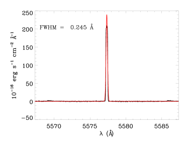
Figure D.1: VLT-UVES instrumental profile and its gaussian fit, as obtained from the OI 5577 Å sky line. The observed line is shown in black and the gaussian fit in red. This, as all the following profiles, is shown in a 20 Å wide window.

Figure D.2: H$\beta$ lines best fits for VLT UVES data. The observed $\mathrm{H}\beta$ line and the three different fits are shown in a 20 Å wide window for each object as labelled. Upper panel: The single gaussian fit is indicated by a dashed line (thick black),the asymmetric gaussian fit is indicated by a dash-dotted line (blue) and the three separate gaussians fit is indicated by long-dashed lines (red) with its total fit shown by a dash-double-dotted line (yellow); the parameters of the fits are listed in the top left corner. Lower panel: Shows the residuals from the fitting procedures following the same colour code with crosses for the single gaussian fit and continuous lines both for the asymmetric and three gaussian fits. The inset shows the results from the Montecarlo simulation to estimate the errors in the FWHM of the best fit. Details are described in the main text.

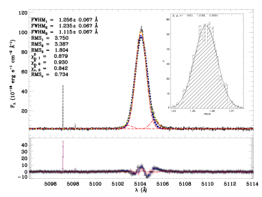
(a) J051519-391741

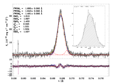
(b) J074806+193146

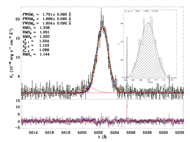
(c) J074947+154013

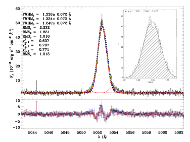
(d) J080000+274642

Figure D.3: H$\beta$ lines best fits continued.

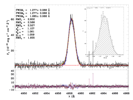
(a) J081403+235328

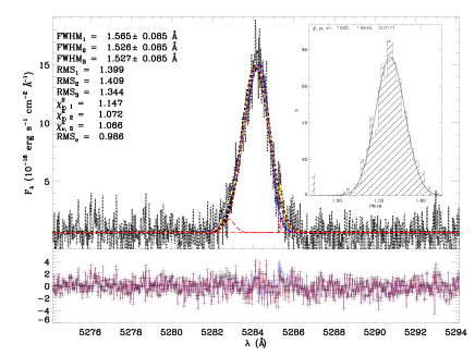
(b) J082520+082723

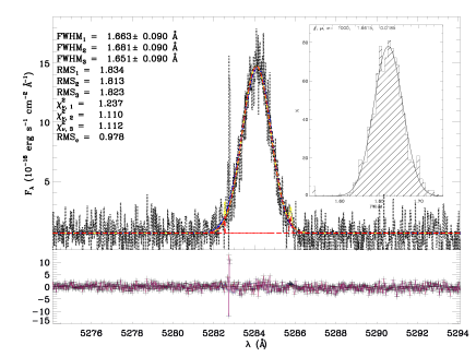
(c) J082520+082723

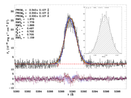
(d) J082722+202612

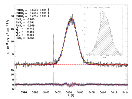
(e) J083946+140033

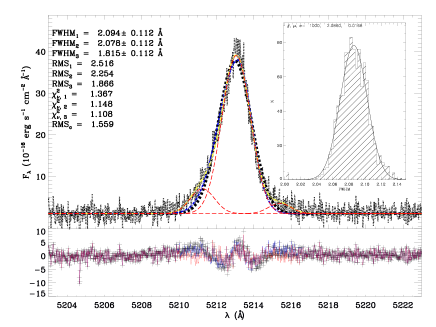
(f) J084000+180531

List of Figures

1. 2.1 Supernovae Ia Hubble Diagram
2. 2.2 Acoustic temperature spectrum sensitivity
3. 2.3 Angular power spectrum measurements
4. 2.4 Angular power spectrum from Planck
5. 2.5 BAO peak in clustering of red galaxies
6. 2.6 Union2 compilation Hubble diagram
7. 2.7 Constraints on cosmological parameters
8. 3.1 H ii galaxies abundances
9. 3.2 $L-\sigma$ relation from Melnick, Terlevich & Terlevich (2000)
10. 3.3 Differential Hubbel diagram for H ii galaxies
11. 3.4 $M(B)_{0}-\sigma$ Relation
12. 3.5 H ii galaxies Fundamental Plane
13. 3.6 Distance Modulus Differences
14. 3.7 Cosmological Parameters Solution Space
15. 3.8 Cosmological Parameters Solution Space from Monte-Carlo Analysis
16. 3.9 Cosmological Parameters Solution Space from Monte-Carlo Analysis 2
17. 4.1 Redshift distribution of the sample
18. 4.2 $\mathrm{H}\beta$ equivalent width distribution for the sample.
19. 4.3 Evolution of the $\mathrm{H}\beta$ equivalent width for an instantaneous starburst
20. 4.4 Selection of colour images of H ii galaxies
21. 4.5 Examples of the high dispersion spectra
22. 4.6 An example of gaussian fit and integration under the emission line
23. 4.7 Fluxes measured from SDSS
24. 4.8 BPT diagram of a sample of H ii galaxies
25. 4.9 Typical multiple gaussian fit to an $\mathrm{H}\beta$ line
26. 4.10 Comparison of $\sigma$ values after applying broadening corrections
27. 4.11 Distribution of the $\mathrm{H}\beta$ velocity dispersion
28. 4.12 Distribution of the $\mathrm{H}\beta$ emission line luminosities
29. 4.13 Luminosity function for our sample of H ii galaxies
30. 4.14 Distribution of oxygen abundances for the sample S3
31. 4.15 Comparison between $M_{cl}+M_{ion}$ and $M_{dyn}$
32. 4.16 The continuum luminosity-metallicity relation for S3
33. 4.17 The $\mathrm{H}\beta$ luminosity-metallicity relation for S3
34. 4.18 The EW($\mathrm{H}\beta$) - metallicity relation for S3
35. 4.19 Automatic profile selection
36. 4.20 $L-\sigma$ relation for all the H ii galaxies
37. 4.21 Observed L(H$\beta$) vs. calculated using the best Bayesian multi-parametric fitting
38. 5.1 $L(\mathrm{H}\beta)-\sigma$ relation for the GEHR sample
39. 5.2 $L(\mathrm{H}\beta)-\sigma$ relation for the joint H ii galaxies and GEHR sample
40. 5.3 Values of $\chi^{2}$ for the grid of $H_{0}$
41. 5.4 Hubble diagram for our sample of 69 H ii galaxies
42. 6.1 Typical gaussian fit to a resolved emission line
43. 6.2 $L-\sigma$ relation for the combined local and high-z samples of H ii galaxies
44. 6.3 Typical gaussian fit to a resolved emission line
45. 6.4 Solution spaces for $\mathbf{p}=\{H_{0},\Omega_{m}\}$
46. 6.5 Solution spaces for $\mathbf{p}=\{\Omega_{m},w_{0}\}$
47. 6.6 Solution spaces for $\mathbf{p}=\{w_{0},w_{1}\}$
48. 6.7 Comparison on restrictions of the plane $\mathbf{p}=\{\Omega_{m},w_{0}\}$
49. 6.8 Comparison on restrictions of the plane $\mathbf{p}=\{\Omega_{m},w_{0}\}$
50. B.1 Trigonometric Parallax scheme
51. B.2 Moving-cluster method scheme
52. D.1 VLT-UVES instrumental profile
53. D.2 H$\beta$ lines best fits for VLT UVES data
54. D.3 H$\beta$ lines best fits continued.

List of Tables

1. 2.1 Cosmological parameters fit from Union2.1
2. 3.1 Cosmological parameters fits from SNe Ia
3. 4.2 Observations and Data Reduction
4. 4.3 Data Analysis.
5. 4.3 Local H ii galaxies Fluxes and EW
6. 4.4 Local H ii galaxies line intensity ratios
7. 4.5 Local H ii galaxies FWHMs
8. 4.6 Local H ii galaxies derived values
9. 4.5.2 Further restricting the sample by the quality of the line profile fits
10. 4.5.3 Search for a second parameter in the $L(\mathrm{H}\beta)-\sigma$ relation
11. 4.5.3 Search for a second parameter in the $L(\mathrm{H}\beta)-\sigma$ relation
12. 4.5.3 Search for a second parameter in the $L(\mathrm{H}\beta)-\sigma$ relation
13. Metallicity
14. Metallicity
15. 4.13 Regression coefficients for S3
16. 4.14 Bayesian Regression coefficients for S3
17. 4.15 Regression coefficients for S3 using $\sigma([\mathrm{OIII}])$
18. 4.16 Bayesian regression coefficients for S3 and using $\sigma([\mathrm{OIII}])$
19. 4.5.4 Multiparametric fits
20. 4.5.4 Multiparametric fits
21. 5.1 Distance Moduli for the GEHR sample
22. 5.2.1 Systematics
23. 6.1 High-$z$ sample FWHM
24. 6.2 High-$z$ H ii galaxies parameters adopted values

References

- Aad et al. (2012) Aad G. et al., 2012, Physics Letters B, 716, 1
- Aaronson et al. (1986) Aaronson M., Bothun G., Mould J., Huchra J., Schommer R. A., Cornell M. E., 1986, ApJ, 302, 536
- Aaronson, Huchra & Mould (1979) Aaronson M., Huchra J., Mould J., 1979, ApJ, 229, 1
- Abazajian et al. (2009) Abazajian K. N. et al., 2009, ApJS, 182, 543
- Aguirre (1999) Aguirre A., 1999, ApJ, 525, 583
- Albrecht et al. (2006) Albrecht A. et al., 2006, ArXiv:astro-ph/0609591
- Alcock et al. (1997) Alcock C. et al., 1997, ApJ, 482, 89
- Alcock & et al. (2004) Alcock C., et al., 2004, AJ, 127, 334
- Alloin, Bergeron & Pelat (1978) Alloin D., Bergeron J., Pelat D., 1978, A&A, 70, 141
- Amanullah et al. (2010) Amanullah R. et al., 2010, ApJ, 716, 712
- An, Terndrup & Pinsonneault (2007) An D., Terndrup D. M., Pinsonneault M. H., 2007, ApJ, 671, 1640
- Andernach et al. (2005) Andernach H., Plionis M., López-Cruz O., Tago E., Basilakos S., 2005, in Astronomical Society of the Pacific Conference Series, Vol. 329, Nearby Large-Scale Structures and the Zone of Avoidance, A. P. Fairall & P. A. Woudt, ed., pp. 289–293
- Anderson et al. (2014) Anderson L. et al., 2014, MNRAS, 441, 24
- Astier et al. (2006) Astier P. et al., 2006, A&A, 447, 31
- Atek et al. (2010) Atek H. et al., 2010, ApJ, 723, 104
- Barlow (2004) Barlow R., 2004, ArXiv: physics/0406120
- Basilakos & Plionis (1998) Basilakos S., Plionis M., 1998, MNRAS, 299, 637
- Basilakos & Plionis (2006) Basilakos S., Plionis M., 2006, MNRAS, 373, 1112
- Basilakos, Plionis & Solà (2009) Basilakos S., Plionis M., Solà J., 2009, Phys. Rev. D, 80, 083511
- Bellazzini (2008) Bellazzini M., 2008, Memorie della Societa Astronomica Italiana, 79, 440
- Benedict & et al. (2002a) Benedict G. F., et al., 2002a, AJ, 124, 1695
- Benedict & et al. (2002b) Benedict G. F., et al., 2002b, AJ, 123, 473
- Benedict et al. (2007a) Benedict G. F. et al., 2007a, AJ, 133, 1810
- Benedict et al. (2007b) Benedict G. F. et al., 2007b, AJ, 133, 1810
- Bergeron (1977) Bergeron J., 1977, ApJ, 211, 62
- Beutler et al. (2011) Beutler F. et al., 2011, MNRAS, 416, 3017
- Binney & Merrifield (1998) Binney J., Merrifield M., 1998, Galactic Astronomy. Princeton University Press
- Binney & Tremaine (1987) Binney J., Tremaine S., 1987, Galactic dynamics. Princeton University Press
- Birkinshaw (1999) Birkinshaw M., 1999, Phys. Rep., 310, 97
- Bohm-Vitense (1997) Bohm-Vitense E., 1997, AJ, 113, 13
- Bonamente et al. (2006) Bonamente M., Joy M. K., LaRoque S. J., Carlstrom J. E., Reese E. D., Dawson K. S., 2006, ApJ, 647, 25
- Bonanos et al. (2006) Bonanos A. Z. et al., 2006, ApJ, 652, 313
- Bono et al. (1999) Bono G., Caputo F., Castellani V., Marconi M., 1999, ApJ, 512, 711
- Bono et al. (2008) Bono G., Caputo F., Fiorentino G., Marconi M., Musella I., 2008, ApJ, 684, 102
- Bono, Castellani & Marconi (2002) Bono G., Castellani V., Marconi M., 2002, ApJ, 565, L83
- Bono et al. (2002) Bono G., Groenewegen M. A. T., Marconi M., Caputo F., 2002, ApJ, 574, L33
- Bordalo & Telles (2011) Bordalo V., Telles E., 2011, ApJ, 735, 52
- Borissova et al. (2004) Borissova J., Minniti D., Rejkuba M., Alves D., Cook K. H., Freeman K. C., 2004, A&A, 423, 97
- Borissova et al. (2009) Borissova J., Rejkuba M., Minniti D., Catelan M., Ivanov V. D., 2009, A&A, 502, 505
- Bradley et al. (2006) Bradley T. R., Knapen J. H., Beckman J. E., Folkes S. L., 2006, A&A, 459, L13
- Brosch, Almoznino & Heller (2004) Brosch N., Almoznino E., Heller A. B., 2004, MNRAS, 349, 357
- Caldwell & Kamionkowski (2009) Caldwell R. R., Kamionkowski M., 2009, Annual Review of Nuclear and Particle Science, 59, 397
- Calzetti et al. (2000) Calzetti D., Armus L., Bohlin R. C., Kinney A. L., Koornneef J., Storchi-Bergmann T., 2000, ApJ, 533, 682
- Campos-Aguilar, Moles & Masegosa (1993) Campos-Aguilar A., Moles M., Masegosa J., 1993, AJ, 106, 1784
- Carlstrom, Holder & Reese (2002) Carlstrom J. E., Holder G. P., Reese E. D., 2002, ARA&A, 40, 643
- Carroll (2001) Carroll S. M., 2001, Living Reviews in Relativity, 4, 1
- Carroll et al. (2004) Carroll S. M., Duvvuri V., Trodden M., Turner M. S., 2004, Phys. Rev. D, 70, 043528
- Catelan & Cortés (2008) Catelan M., Cortés C., 2008, ApJ, 676, L135
- Chávez et al. (2012) Chávez R., Terlevich E., Terlevich R., Plionis M., Bresolin F., Basilakos S., Melnick J., 2012, MNRAS, 425, L56
- Chávez et al. (2014) Chávez R., Terlevich R., Terlevich E., Bresolin F., Melnick J., Plionis M., Basilakos S., 2014, MNRAS, 442, 3565
- Chevallier & Polarski (2001) Chevallier M., Polarski D., 2001, International Journal of Modern Physics D, 10, 213
- Clausen et al. (2003) Clausen J. V., Storm J., Larsen S. S., Giménez A., 2003, A&A, 402, 509
- Clement, Xu & Muzzin (2008) Clement C. M., Xu X., Muzzin A. V., 2008, AJ, 135, 83
- Clementini et al. (2003a) Clementini G., Gratton R., Bragaglia A., Carretta E., Di Fabrizio L., Maio M., 2003a, AJ, 125, 1309
- Clementini et al. (2003b) Clementini G., Held E. V., Baldacci L., Rizzi L., 2003b, ApJ, 588, L85
- Cole (1998) Cole A. A., 1998, ApJ, 500, L137
- Conley et al. (2011) Conley A. et al., 2011, ApJS, 192, 1
- Copeland, Sami & Tsujikawa (2006) Copeland E. J., Sami M., Tsujikawa S., 2006, International Journal of Modern Physics D, 15, 1753
- Copetti, Pastoriza & Dottori (1986) Copetti M. V. F., Pastoriza M. G., Dottori H. A., 1986, A&A, 156, 111
- Courteau & van den Bergh (1999) Courteau S., van den Bergh S., 1999, AJ, 118, 337
- Dalcanton & et al. (2009) Dalcanton J. J., et al., 2009, ApJS, 183, 67
- Dall’Ora et al. (2004) Dall’Ora M. et al., 2004, ApJ, 610, 269
- Davis et al. (2007) Davis T. M. et al., 2007, ApJ, 666, 716
- Deb & Singh (2010) Deb S., Singh H. P., 2010, MNRAS, 402, 691
- Deffayet (2001) Deffayet C., 2001, Physics Letters B, 502, 199
- Dekker et al. (2000) Dekker H., D’Odorico S., Kaufer A., Delabre B., Kotzlowski H., 2000, in Society of Photo-Optical Instrumentation Engineers (SPIE) Conference Series, Vol. 4008, Society of Photo-Optical Instrumentation Engineers (SPIE) Conference Series, M. Iye & A. F. Moorwood, ed., pp. 534–545
- di Benedetto (1995) di Benedetto G. P., 1995, ApJ, 452, 195
- di Benedetto (1997) di Benedetto G. P., 1997, ApJ, 486, 60
- Díaz et al. (2000) Díaz A. I., Álvarez M. Á., Terlevich E., Terlevich R., Sánchez Portal M., Aretxaga I., 2000, MNRAS, 311, 120
- Dicus & Repko (2004) Dicus D. A., Repko W. W., 2004, Phys. Rev. D, 70, 083527
- Dolphin et al. (2003) Dolphin A. E. et al., 2003, AJ, 125, 1261
- Dottori (1981) Dottori H. A., 1981, Ap&SS, 80, 267
- Dottori & Bica (1981) Dottori H. A., Bica E. L. D., 1981, A&A, 102, 245
- Doublier et al. (1997) Doublier V., Comte G., Petrosian A., Surace C., Turatto M., 1997, A&AS, 124, 405
- Drell, Loredo & Wasserman (2000) Drell P. S., Loredo T. J., Wasserman I., 2000, ApJ, 530, 593
- Dvali, Gabadadze & Porrati (2000) Dvali G., Gabadadze G., Porrati M., 2000, Physics Letters B, 485, 208
- Efstathiou, Sutherland & Maddox (1990) Efstathiou G., Sutherland W. J., Maddox S. J., 1990, Nature, 348, 705
- Eisenstein et al. (2005) Eisenstein D. J. et al., 2005, ApJ, 633, 560
- Erb et al. (2003) Erb D. K., Shapley A. E., Steidel C. C., Pettini M., Adelberger K. L., Hunt M. P., Moorwood A. F. M., Cuby J., 2003, ApJ, 591, 101
- Erb et al. (2006a) Erb D. K., Steidel C. C., Shapley A. E., Pettini M., Reddy N. A., Adelberger K. L., 2006a, ApJ, 647, 128
- Erb et al. (2006b) Erb D. K., Steidel C. C., Shapley A. E., Pettini M., Reddy N. A., Adelberger K. L., 2006b, ApJ, 646, 107
- Evans et al. (2013) Evans C. et al., 2013, ArXiv: astro-ph/303.0029
- Faber & Jackson (1976) Faber S. M., Jackson R. E., 1976, ApJ, 204, 668
- Feast (1999) Feast M., 1999, PASP, 111, 775
- Feast (2005) Feast M., 2005, in Astronomical Society of the Pacific Conference Series, Vol. 329, Nearby Large-Scale Structures and the Zone of Avoidance, Fairall A. P., Woudt P. A., eds., p. 241
- Feast (1997) Feast M. W., 1997, MNRAS, 284, 761
- Feast & Catchpole (1997) Feast M. W., Catchpole R. M., 1997, MNRAS, 286, L1
- Feast et al. (2012) Feast M. W., Whitelock P. A., Menzies J. W., Matsunaga N., 2012, MNRAS, 421, 2998
- Fernley et al. (1998) Fernley J., Barnes T. G., Skillen I., Hawley S. L., Hanley C. J., Evans D. W., Solano E., Garrido R., 1998, A&A, 330, 515
- Ferrarese et al. (2000) Ferrarese L. et al., 2000, ApJS, 128, 431
- Fitzpatrick et al. (2002) Fitzpatrick E. L., Ribas I., Guinan E. F., DeWarf L. E., Maloney F. P., Massa D., 2002, ApJ, 564, 260
- Fitzpatrick et al. (2003) Fitzpatrick E. L., Ribas I., Guinan E. F., Maloney F. P., Claret A., 2003, ApJ, 587, 685
- Fixsen et al. (1996) Fixsen D. J., Cheng E. S., Gales J. M., Mather J. C., Shafer R. A., Wright E. L., 1996, ApJ, 473, 576
- Fouqué et al. (2007a) Fouqué P. et al., 2007a, A&A, 476, 73
- Fouqué et al. (2007b) Fouqué P. et al., 2007b, A&A, 476, 73
- Freedman & Madore (2010) Freedman W. L., Madore B. F., 2010, ARA&A, 48, 673
- Freedman et al. (2001) Freedman W. L. et al., 2001, ApJ, 553, 47
- Freedman et al. (2012) Freedman W. L., Madore B. F., Scowcroft V., Burns C., Monson A., Persson S. E., Seibert M., Rigby J., 2012, ApJ, 758, 24
- French (1980) French H. B., 1980, ApJ, 240, 41
- Frieman et al. (2003) Frieman J. A., Huterer D., Linder E. V., Turner M. S., 2003, Phys. Rev. D, 67, 083505