A Novel Non-Parametric Approach to Compare Paired General Statistical Distributions between Two Interventions

Abstract

Despite of many measures applied for determine the difference between two groups of observations, such as mean value, median value, sample standard deviation and so on, we propose a novel non parametric transformation method based on Mallows distance to investigate the location and variance differences between the two groups. The convexity theory of this method is constructed and thus it is a viable alternative for data of any distributions. In addition, we are able to establish the similar method under other distance measures, such as Kolmogorov-Smirnov distance. The application of our method in real data is performed as well.

1 INTRODUCTION

The aim of this paper is to provide a method to determine the location and scale relationship between two groups of one-dimensional observations for two samples, say $\{X_{1},X_{2},...,X_{n}\}$ and $\{Y_{1},Y_{2},...,Y_{m}\}$, such as the responses of two different products on different subjects, the scores of people on two examinations and so on. Suppose $\{X_{i}\}$ are independent identity distributed according to $F(\cdot)$ and $\{Y_{i}\}$ are independent identity distributed according to $G(\cdot)$, where $F(\cdot)$ and $G(\cdot)$ are two unknown distribution functions. When the test for normality is not passed, nonparametric analysis methods should be applied. Usually, the mean difference or midian difference of the two samples is used to determine the location difference and use mean ratio or midian ratio to obtain the scale. They are not reliable since only a small information of the two samples are extracted and the results are not meaningful.

Based on the idea of location-scale transformation, Freitag, Munk and Vogt [1] has developed an approach to access the structure relationship between distributions, in which the whole information of the samples are used. However, the problem we concern are the location difference and scale between two distributions rather than the model structure. That’s to say, we have to determine the values of location difference or scale or both for any two distributions. Using the same transformation idea, our approach can be described as follows.

Let $\phi(\cdot)$ a linear function, i.e., $\phi(x)=\sigma x+h$, where $\sigma>0$ and $h\in(-\infty,+\infty)$. $d$ is a given measure of discrepancy between two distributions. Denote the distribution function of $\phi(X_{i})$ by $F_{1}$. Let $D(\sigma,h)=d(F_{1},G)$. We want to find the value $(\sigma_{0},h_{0})$ which minimize $D(\sigma_{0},h_{0})$. That’s to say, if we transform $\{X_{i}\}$ to be $\sigma_{0}X_{i}+h_{0}$ , the two groups of observations are closest and under the ”closest” mean we can not tell there are any location difference or scale between them. Therefore, we can say $\{Y_{i}\}$ is at least $h_{0}$ larger than $\sigma_{0}$ times of $\{X_{i}\}$.

There are situations where $(\sigma_{0},h_{0})$ is not unique. Let $S=\mbox{argmin}_{(\sigma,h)}D(\sigma,h)$, $S_{\sigma}=\{\sigma:\exists h,~{}(\sigma,h)\in S\}$ and $S_{h|\sigma}=\{h:(\sigma,h)\in S\}$. Conservatively, at first we can take $\sigma_{0}=1$ if $1\in S_{\sigma}$, else $\sigma_{0}=\inf S_{\sigma}$; then take $h_{0}$ to be the value in $S_{h|\sigma_{0}}$ satisfying $|h_{0}|=\inf\{|h|:h\in S_{h|\sigma_{0}}\}$. When $S$ is a continues region, it is easy to see that the selected $(\sigma_{0},h_{0})$ is unique. Therefore, we should find certain $d$ that $S$ is a continues region.

Besides, if we let $\sigma\equiv 1$ in $D(\sigma,h)$, the location difference between $F$ and $G$ could be determined. If we let $h\equiv 0$ in $D(\sigma,h)$, the scale between $F$ and $G$ could be determined. In practice, we could use the empirical distributions of the two group of data for $F(\cdot)$ and $G(\cdot)$, respectively. The discrepancy measure $d$ we consider in this paper will be focused on Mallows Distance and expand to Kolmogorov-Smirnov Distance. Mallows Distance was presented in the formulation of statistics framework in 1972, however, an independent physics research work had involved such a related concept a little earlier in 1940s.

The rest of the paper is unfolded as follows. In Section 2 the main results under Mallows Distance for the location transformation, scale transformation or both are presented, showing that we can uniquely determine the location and scale relationship between two distributions and thus Mallows Distance is suitable discrepancy measure to use. In Section 3 the similar results can be obtained under Kolmogorov-Smirnov Distance but only for location transformation. Section 4 gives the application of this approach to determine the location and scale relationship on real data.

2 MATHEMATICAL FORMULA

2.1 Definition of Mallows Distance

In this subsection, we consider the proposed approach under Mallows Distance. Formally, The Mallows $r$-distance (also known as Wasserstein $r$-distance) between distributions $F(\cdot)$ and $G(\cdot)$ regarding to random variables $X$ and $Y$, respectively, is defined as

$$d_{r}(F,G)=\inf_{X,Y}(E|X-Y|^{r})^{\frac{1}{r}},$$ (1)

where the infimum is taken over the set (denoted by $\mathbb{D}_{r}$) of all joint distributions of $X$ and $Y$ with marginals $F(\cdot)$ and $G(\cdot)$. Here we require that $X$ and $Y$ have finite $r$th moment, i.e., $E|X|^{r}<\infty$ and $E|Y|^{r}<\infty$.

For $r\geq 1$, The Mallows $r$-distance $d_{r}(F,G)$ has the two properties.

• Mallows distance $d_{r}(F,G)$, i.e. satisfies axioms of a metric on $\mathbb{D}_{r}$.

• The convergence of distributions in Mallows distance is equivalent to weak convergence plus $r$th moment convergence.(Lavina and Bickel, 2001)

Let $U$ be an uniform random variable, $U\sim Unif(0,1)$, and $F^{-1}(\cdot)$ is the inverse of a distribution function, $F^{-1}(u)=\inf_{x}\{x:F(x)\geq u\}$. According to Johnson and Samworth (2005) we know

$$\inf_{X,Y}E|X-Y|^{r}=E|F^{-1}(U)-G^{-1}(U)|^{r}.$$ (2)

Equation (2) gives an easier computation formula to calculate the distance, that is

$$d_{r}(F,G)=\left(\int_{0}^{1}|F^{-1}(u)-G^{-1}(u)|^{r}du\right)^{\frac{1}{r}}.$$ (3)

Particularly, when $r=1$, we have a further relationship for computation

$$d_{1}(F,G)=\int_{0}^{1}|F^{-1}(u)-G^{-1}(u)|du=\int_{-\infty}^{+\infty}|F(x)-G(x)|dx,$$ (4)

which is especially useful when calculating Mallows 1-distance using empirical distribution for real data, in order to circumvent the unknown real distribution.

2.2 Approach under Mallows Distance

Let $\phi(X)=\sigma X+h$, where $\sigma>0$ and $h\in(-\infty,\infty)$, and $F_{1}(\cdot)$ be its distribution function, then it is easy to obtain that $F_{1}(x)=F(\frac{x-h}{\sigma})$. The purpose of our approach is to find the optimal shift and scale values $(\sigma_{0},h_{0})$ to minimizing the Mallows $r$-distance between $F_{1}(x)$ and $G(x)$, that is

$$\arg\min_{\sigma,h}d_{r}(F_{1}(x),G(x)).$$ (5)

Then the following result can be obtained.

Theorem 1.

For distribution functions $F(\cdot)$ and $G(\cdot)$, let $F_{1}(x)=F(\frac{x-h}{\sigma})$ with $\sigma>0$. Then the Mallows $r$-distance ($r\geq 1$) between $F_{1}(x)$ and $G(x)$, denoted by $D(\sigma,h)$, a function of two variables $\sigma$ and $h$, is a continuous and convex function on half plane, i.e., for any $0<t<1$, and $\sigma_{1}\neq\sigma_{2}$, $h_{1}\neq h_{2}$, it holds that

$$D(t\sigma_{1}+(1-t)\sigma_{2},th_{1}+(1-t)h_{2})\leq tD(\sigma_{1},h_{1})+(1-t)D(\sigma_{2},h_{2}).$$

Proof.

It can be easily obtained that $F_{1}^{-1}(u)=\sigma F^{-1}(u)+h$. From (3), we know

$$D(\sigma,h)=\left(\int_{0}^{1}\left|\sigma F^{-1}(u)+h-G^{-1}(u)\right|^{r}du\right)^{\frac{1}{r}}.$$ (6)

Then the continuity of the $D(\sigma,h)$ is trivial. Besides, using Minkowski unequality we have

$$D(t\sigma_{1}+(1-t)\sigma_{2},th_{1}+(1-t)h_{2})$$

$$=\left(\int_{0}^{1}\left|(t\sigma_{1}+(1-t)\sigma_{2})F^{-1}(u)+th_{1}+(1-t)h_{2}-G^{-1}(u)\right|^{r}du\right)^{\frac{1}{r}}$$

$$=\left(\int_{0}^{1}\left|t\left(\sigma_{1}F^{-1}(u)+h_{1}-G^{-1}(u)\right)+(1-t)\left(\sigma_{2}F^{-1}(u)+h_{2}-G^{-1}(u)\right)\right|^{r}du\right)^{\frac{1}{r}}$$

$$\leq t\left(\int_{0}^{1}\left|\left(\sigma_{1}F^{-1}(u)+h_{1}-G^{-1}(u)\right)\right|^{r}du\right)^{\frac{1}{r}}+(1-t)\left(\int_{0}^{1}\left|\left(\sigma_{2}F^{-1}(u)+h_{2}-G^{-1}(u)\right)\right|^{r}du\right)^{\frac{1}{r}}$$

$$=tD(\sigma_{1},h_{1})+(1-t)D(\sigma_{2},h_{2}).$$

∎

According to the definition of Theorem 1, scaled parameter $\sigma$ should be greater than zero, but we can easily give an apparent analysis of transformed distribution function if $\sigma\rightarrow 0^{+}$.

Proposition 1.

$$\lim_{\sigma\rightarrow 0^{+}}F\left(\frac{x+h}{\sigma}\right)=\left\{\begin{aligned} 1&,x>0\\ F(0)&,x=0\\ 0&,x<0\end{aligned}\right.$$

Also, the Theorem shows that under Mallows $r$-distance ($r\geq 1$) $D(\sigma,h)$ is a convex function of $(\sigma,h)$, thus (5) is a continues region. We can select $(\sigma_{0},h_{0})$ according to the plan in section 1. If we only consider the shifted case or scaled case, let $\sigma\equiv 1$ or $h\equiv 0$ in $D(\sigma,h)$, then we can obtain the following results.

Corollary 1.

For distribution functions $F(\cdot)$ and $G(\cdot)$, let $F_{1}(x)=F(x-h)$. Then the Mallows $r$-distance ($r\geq 1$) between $F_{1}(x)$ and $G(x)$, denoted by $D(h)$, a function of $h$, is a continuous and convex function on $(-\infty,\infty)$, i.e. for any $0<t<1$, and $h_{1}\neq h_{2}$, it holds that

$$D(th_{1}+(1-t)h_{2})\leq tD(h_{1})+(1-t)D(h_{2}).$$

Corollary 2.

For distribution functions $F(\cdot)$ and $G(\cdot)$, let $F_{1}(x)=F(\frac{x}{\sigma})$ with $\sigma>0$. The Mallows Distance ($r\geq 1$) between the scaled distribution $F_{1}(x)$ and $G(x)$, denoted as $D(\sigma)$, a function of $\sigma$, is a continuous and convex function on $(0,\infty)$, i.e. for any $0<t<1$, and $\sigma_{1}\neq\sigma_{2}$, it holds that

$$D(t\sigma_{1}+(1-t)\sigma_{2})\leq tD(\sigma_{1})+(1-t)D(\sigma_{2}).$$

In order to illustrate $D(\sigma,h)$ may not be strictly convex, let distributions $F(\cdot)$ and $G(\cdot)$ to be

$$F(x)=\left\{\begin{aligned} 0,&\qquad x\leq-1,\\ linear,&\qquad-1<x<-0.5,\\ 0.5,&\qquad-0.5\leq x\leq 0.5,\\ linear,&\qquad 0.5<x<1,\\ 1,&\qquad x\geq 1,\end{aligned}\right.\qquad\mbox{and}\qquad G(x)=\left\{\begin{aligned} 0,&\qquad x\leq 1,\\ linear,&\qquad 1<x<2,\\ 1,&\qquad x\geq 2.\end{aligned}\right.$$

Actually, $F(\cdot)$ is the uniform distribution over two half unit intervals $[-1,-0.5]$ and $[0.5,1]$, and $G(\cdot)$ is uniform over $[1,2]$. From (4) we know $D(h)$ can be calculated via $\int_{-\infty}^{+\infty}|F(x-h)-G(x)|dx$. Then it is easy to verify that $D(h)$ reaches minimum of 0.5 in the entire interval $[-2,-1]$. The optimal shifted value for $\arg\min_{h}D(h)$ is not unique. Therefore, $D(h)$ is not strictly convex on $(-\infty,\infty)$, nor is $D(\sigma,h)$.

2.3 Generalization on K-S Distances

Since our approach is successful under Mallows distance, there is nothing preventing us from exploring other discrepancy measure. Here, we are able to realize our approach for shifted case under Kolmogorov-Smirnov distance (K-S distance), $D(F,G)=\sup_{x}|F(x)-G(x)|$.

For K-S distance and distribution functions $F(\cdot)$ and $G(\cdot)$, our purpose is to find the optimal shift value $h_{0}$ to minimize $D(h)=\sup_{x}|F(x-h)-G(x)|$. Let $F(\infty)=1$ and $F(-\infty)=0$ for distribution $F$. Define $D^{+}(h)=\sup_{x}[F(x-h)-G(x)]$ and $D^{-}(h)=\sup_{x}[G(x)-F(x-h)]$, then we have $D(h)=\max\{D^{+}(h),D^{-}(h)\}$. And we denote $S=\{h|D(h)=D^{+}(h)\}$ and $h^{*}=\inf S$. Due to these definitions, the statement $-\infty\in S$ is apparently hold and we have the following result.

Theorem 2.

$\mathtt{(1)}$ If $h^{*}\in S$, then the function $D(h)$ decreases on $(-\infty,h^{*}]$ and increases on $(h^{*},+\infty)$. $\mathtt{(2)}$ If $h^{*}\notin S$, then the function $D(h)$ decreases on $(-\infty,h^{*})$ and increases on $[h^{*},+\infty)$.

Proof.

$\mathtt{(1)}$ $\forall h_{0}\in S$, if $h_{2}\leq h_{1}\leq h_{0}$, then we have

$$D(h_{1})\geq D^{+}(h_{1})\geq D^{+}(h_{0})=D(h_{0}).$$ (7)

If $D(h_{1})=D^{-}(h_{1})$, then $D(h_{0})\geq D^{-}(h_{0})\geq D^{-}(h_{1})=D(h_{1})\geq D(h_{0})$ holds and $D(h_{1})=D(h_{0})$. By (7), we can obtain $D(h_{1})=D^{+}(h_{1})$. Thus $D(h_{1})=D^{+}(h_{1})$ and $D(h_{2})\geq D^{+}(h_{2})\geq D^{+}(h_{1})=D(h_{1})$. Therefore, $D(h)$ decreases on $(-\infty,h^{*}]$.

Similarly, $\forall h_{0}\notin S$, if $h_{0}\leq h_{1}\leq h_{2}$, then we have

$$D(h_{1})\geq D^{-}(h_{1})\geq D^{-}(h_{0})=D(h_{0}).$$ (8)

If $D(h_{1})=D^{+}(h_{1})$, then $D(h_{0})\geq D^{+}(h_{0})\geq D^{+}(h_{1})=D(h_{1})\geq D(h_{0})$ holds and $D(h_{1})=D^{+}(h_{0})$. By (8), we can obtain $D(h_{1})=D^{-}(h_{1})$. Thus $D(h_{2})\geq D^{-}(h_{2})\geq D^{-}(h_{1})=D(h_{1})$. Therefore, $D(h)$ increases on $(h^{*},\infty)$.

$\mathtt{(2)}$ The proof can follow the similar method as $\mathtt{(1)}$ trivially. ∎

Theorem 2 shows that our approach under K-S distance can also provide a reasonable, possibly unique location difference between two distributions.

3 EXPERIMENTS AND SIMULATION

3.1 A Real Data Set

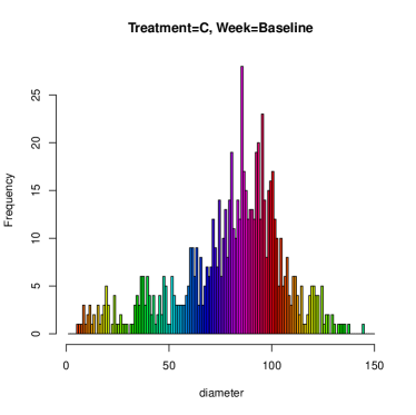
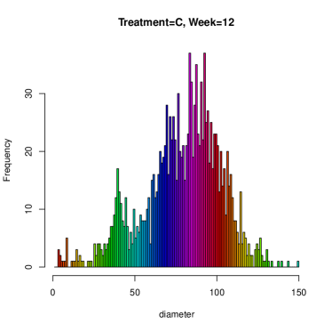
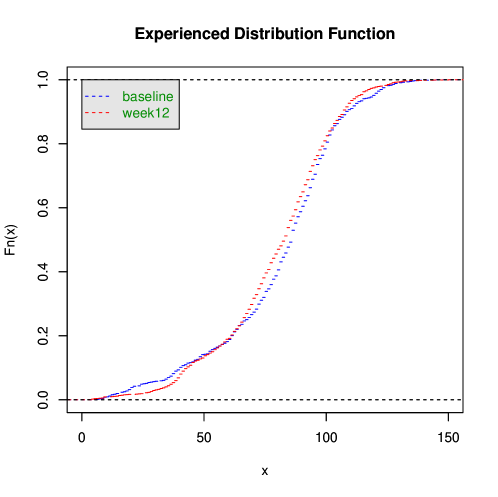
In hair study, we need to assess effets of hair care products in changing hair diameters after a period of use. There are two treatments, say $C$ and $F$. The experiments are conducted as follows. There are 30 subjects and each subject use $C$ and $F$ on the left and right head, respectively. There are two study visit, baseline and 8 weeks later. At each study visit, hair diameters are measured on several hundred of hairs on left and right head from a subject. Comparison between visits is to compare the distributions of hair diameters at two visit point. The diameters from one subject often follows non-traditional distributions. For example, a subject at baseline and 8 weeks later hair diameter frequency plot for treatment $C$ are shown in Figure 1 and the distributions are shown in Figure 2. It is of importance to know holistically how much diameters have changed.

Figure 1: Frequency plot of subject=0001

Figure 2: Distribution of subject=0001

For each subject, the optimal shift amount of the distributions of hair diameters at the two visit point for each treatment under Mallows distance and K-S distance can be obtained. For instance, the shift plots for $C$ and $F$ of a subject are displayed in Figure 3 and shift plots of all subjects for $C$ are displayed in Figure 4 . The shift corresponding to the minimum distance is the difference between two distributions, for comparison analysis.

Figure 3: Shift plot of subject=0001

Figure 4: Shift plot of all subject for $C$

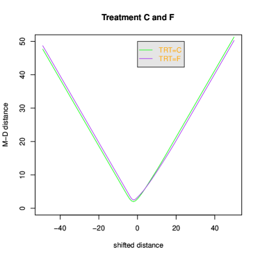
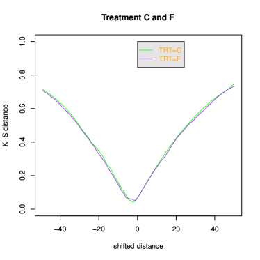
Use the optimal values for each subject each treatment as responses and perform Wilcoxon signed rank test on differences in shifts between treatments for all subjects to detect a difference between the treatments. The results are shown in Table 1, from which we concludes that the two treatments are difference at 0.01 level.

Table 1: Comparison of treatments under Distance Shift

Method	n	Mean.C	Mean.F	Mean.(C-F)	variance.of.diff	p-value
M-D	38	1.395	-0.669	2.065	16.55	0.0030
K-S	38	1.289	-0.763	2.053	19.02	0.0025

3.2 A Simulation Study

We apply computer simulation to illustrate our approach on the shift case, scale case, and shift-scale case under Mallows distance or K-S distance. Let $n=100$ and generates two group of independent data $\{X_{i}\}$ and $\{Y_{i}\}$, where $X_{i}\sim N(\mu_{1},\sigma_{1}^{2})$ and $Y_{i}\sim N(\mu_{2},\sigma_{2}^{2})$, $i=1,2,...,n$. Apply our methods proposed to those data, and calculate the optimal shift value, the optimal scale value and optimal shift-scale values of the three cases. Repeat this process $M=100$ times and the means and standard errors of those calculated values are output.

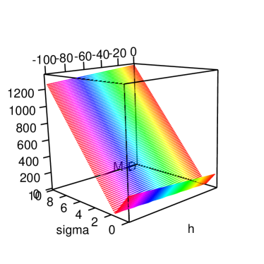
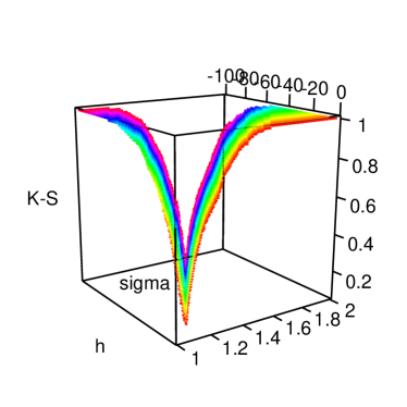
Consider the following four situations: (1) $\mu_{1}=\mu_{2}=150,\sigma_{1}=10,\sigma_{2}=15$; (2) $\mu_{1}=150,\mu_{2}=160,\sigma_{1}=\sigma_{2}=10$; (3) $\mu_{1}=150,\mu_{2}=160,\sigma_{1}=10,\sigma_{2}=15$. The shift-scale plots for Mallows distance and K-S distance in situations (4) are displayed in Figure 5 and the results for all are show in Table 2. We can see that our approach performed better under Mallows distance than K-S distance for all situations and cases except for shift case in situation (1), thus our approach is more robust under Mallows distance than K-S distance. Also, we could demonstrate that the convexity for Mallows distance holds while K-S distance does not, which is consistent with Theorem 1 and 2. However, both their minimization exist and can be computed.

Figure 5: shift-scale plots for Mallows and K-S distance

Table 2: Simulation results: means and standard errors

Situations	(1)		(2)		(3)
	M-D	K-S	M-D	K-S	M-D	K-S
shift	0.11	0.04	10.01	9.93	10.01	9.85
$h_{0}$	(2.0)	(1.9)	(1.3)	(1.4)	(2.0)	(2.0)
scale	1.00	1.00	1.09	1.09	1.09	1.09
$\sigma_{0}$	(0.0)	(0.0)	(0.02)	(0.02)	(0.02)	(0.02)
shift-scale	1.46,-69.03	1.45, -67.75	1.00, 10.00	1.01, 8.45	1.44,-55.9	1.43, -54.93
$\sigma_{0},h_{0}$	(0.1,15.3)	(0.1,16.5)	(0.1,15.6)	(0.1,19.7)	(0.1,18.1)	(0.1,18.8)

4 CONCLUSION AND FUTURE WORK

In this paper, we demonstrated a significant theorem relating to how to measure two distribution within the probabilistic interpretation under Mallows distance or K-S distance, and a well studied simulation on real data had been implemented for an illustration of this method. The solid theoretical foundation would be beneficial to others who would have a further understanding or research on Mallows distance measures the discrepancy between two distributions, especially two similar distributions with inner relationship.

Besides those distances, there might be possibility to use other divergence measures to be minimized after proper transformations. Comparison among various underlying divergence measures will be of interest. This is an area of research that we continue to pursue provided available resources and interests. In addition, A comparison of this approach versus other methods is another topic to be investigated.

References

- [1] Freitag, G., Munk, A., Vogt, M. 2003. Assessing structural relationships between distributions - a quantile process approach based on Mallow’s distance. In: Recent Advances and Trends in Nonparametric Statistics. Ed.: Akritas, M. G., Politis, D. N., Amsterdam: Elsevier B. V., 123-137.
- [2] Mallows, C. L. 1972. A note on asymptotic joint normality.Annals of Mathematical Statistics, 43, 508-515.
- [3] Werman, M., Peleg, S., and Rosenfeld, A. 1985. A distance metric for multidimensional histograms. Computer vision, graphics, and image processing, 32, 328-336
- [4] Bickel, P. and Freedman, D. 1981. Some asymptotic theory for the bootstrap. Ann. Statist., 9, 1196-1217
- [5] Johnson, O. and Samworth, R. 2005. Central limit theorem and convergence to stable laws in Mallows distance. Bernoulli, 11, 829-845
- [6] Levina, E. and Bickel, P. 2001. The earth mover’s distance is the Mallows distance: some insights from statistics. Proceedings IEEE International Conference on Computer Vision
- [7] Anderson, M.J. 2001. A new method for non-parametric multivariate analysis of variance. Austral Ecology, 26, 32-46
- [8] McArdel, B. and Anderson, M.J. 2001. Fitting multivariate models to community data: a comment on distance-based redundancy analysis. Ecology 82, 290-297
- [9] Kosmelj, K. and Billard, L. 2011.Clustering of population pyramids using Mallows L2 distance. Metodoloski zvezki, 8, 1-15