Bending branes for DCFT in two dimensions

Abstract

We consider a holographic dual model for defect conformal field theories (DCFT) in which we include the backreaction of the defect on the dual geometry. In particular, we consider a dual gravity system in which a two-dimensional hypersurface with matter fields, the brane, is embedded into a three-dimensional asymptotically Anti-de Sitter spacetime. Motivated by recent proposals for holographic duals of boundary conformal field theories (BCFT), we assume the geometry of the brane to be determined by Israel junction conditions. We show that these conditions are intimately related to the energy conditions for the brane matter fields, and explain how these energy conditions constrain the possible geometries. This has implications for the holographic entanglement entropy in particular. Moreover, we give exact analytical solutions for the case where the matter content of the brane is a perfect fluid, which in a particular case corresponds to a free massless scalar field. Finally, we describe how our results may be particularly useful for extending a recent proposal for a holographic Kondo model.

1 Introduction

There are important examples of physical systems which contain degrees of freedom confined to a lower-dimensional subspace of spacetime and can be described by conformal field theories. This was studied in particular for CFT in 1+1 dimensions, where often the defect may be described in terms of a boundary condition Affleck:1995ge . In the case where the ambient degrees of freedom are strongly coupled even without the defect, it is natural to expect that applying the AdS/CFT correspondence Maldacena:1997re ; Gubser:1998bc ; Witten:1998qj or one of its extensions will also prove very useful in this context.

The most general holographic approach for studying defect conformal field theory (DCFT) is to consider ‘Janus’ solutions in supergravity, which may be embedded in string theory Aharony:2003qf ; Bak:2003jk ; D'Hoker:2007xy (for recent work see Chiodaroli:2012vc ; Chiodaroli:2011fn ; Gutperle:2012hy ; Jensen:2013lxa ; Dias:2013bwa ; Korovin:2013gha ; Estes:2014hka ; Azeyanagi:2007qj ; Bak:2011ga ; Bak:2007jm ). The Janus configurations amount to a $d$-dimensional domain wall embedded in AdS_d+1, for which the field theory defect dissolves smoothly in the interior of the spacetime. Due to the non-local structure of these configurations, the calculation of physical observables is involved in this approach and generally involves PDE’s.

Recently, there has been interest in the holographic study of boundary conformal field theories (BCFT) and defect conformal field theories (DCFT) in a simpler approach where the gravity dual of the boundary or defect is taken to be a localised infinitesimally thin $d$-dimensional surface in AdS_d+1 Takayanagi:2011zk ; Fujita:2011fp ; Nozaki:2012qd . These models were generalised to holographic models of boundary RG flows, where ‘boundary’ refers to the field theory boundary degrees of freedom rather than to the AdS boundary Takayanagi:2011zk ; Fujita:2011fp ; Nakayama:2012ed . It was shown that these flows satisfy a holographic version of the g-theorem, which states that the boundary entropy decreases along an RG flow from a UV to an IR fixed point Takayanagi:2011zk ; Fujita:2011fp ; Nozaki:2012qd ; Nakayama:2012ed . Within field theory, this theorem was given in Affleck:1991tk ; Friedan:2003yc .

Gravity duals of DCFT in which the dual of the defect remains localised were recently used also for holographic models of the quantum Hall effect. Recent examples include both bottom-up models Melnikov:2012tb ; Lippert:2014jma and top-down models involving brane constructions Kristjansen:2013hma ; Bergman:2010gm . For example, these models display incompressible states with quantised Hall conductivity.

In this paper, we find explicit solutions of the models of Takayanagi:2011zk ; Fujita:2011fp ; Nozaki:2012qd for non-trivial field content. We refer to the localised gravity dual of the field theory defect as the brane, and find explicit solutions which take the backreaction of the brane matter fields on the geometry into account. We construct holographic duals for DCFT by gluing together two a priori distinct asymptotically AdS manifolds. For this to be consistent with the Einstein field equations, the system has to obey the Israel junction conditions Israel:1966rt . These relate the exterior curvature and the induced metric of the brane with the energy-momentum tensor constrained to it. The defect energy-momentum tensor is dynamically generated by matter fields on the brane, subject to appropriate energy conditions. Throughout the paper, we will always assume the null energy condition (NEC) to be satisfied and also investigate the impact of the strong (SEC) and weak energy condition (WEC).

In the AdS/BCFT models mentioned above Takayanagi:2011zk ; Fujita:2011fp ; Nozaki:2012qd , von Neumann boundary conditions are imposed on the brane and, as usual, Dirichlet conditions on the conformal boundary. This ansatz yields the same equations of motion as the use of Israel junction conditions together with the assumption that there is a reflection symmetry around the brane. This is analogous to classical electrodynamics, where von Neumann boundary conditions may be imposed by introducing mirror charges.

Moreover, in this paper we use the Israel junction conditions to link energy conditions imposed on the brane matter to qualitative statements about the exterior geometry of its embedding into the ambient spacetime. In particular, we make use of the so-called ‘barrier theorem’ recently proved by Engelhardt and Wall in Engelhardt:2013tra . This theorem states under which conditions the brane may be intersected by spacelike hypersurfaces which are anchored at the boundary of the manifold. We find a connection between the assumption made for this theorem and a specific combination of energy conditions, which can also be used to distinguish between hypersurface configurations which are anchored twice at the boundary, and others which are infinitely extended into the bulk.

We obtain analytic solutions for the embedding functions for the cases of a constant brane tension, as well as for perfect fluids and a free massless scalar field in $\text{AdS}_{3}$ and BTZ backgrounds. We find that the constant tension solutions may be generated by following a normal flow starting from the trivial solution in a non-backreacting geometry.

Our main motivation to study the models presented, with bulk spacetimes to both sides of the brane, is the holographic bottom-up model for the Kondo effect proposed in Erdmenger:2013dpa , in which a magnetic impurity with $SU(N)$ spin interacts with a strongly coupled field theory. This model is based on a 1+1-dimensional brane with matter fields that extends radially from the AdS boundary into the bulk, in a BTZ black hole spacetime. In the holographic model of Erdmenger:2013dpa , the formation of the Kondo screening cloud corresponds to the formation of a condensate involving an electron and a slave fermion, as realised in field theory for large $N$ Kondo models for instance in Coleman:1986dva ; PhysRevB.35.5072 ; PhysRevLett.90.216403 ; PhysRevB.69.035111 . Moreover, this model involves the gravity dual of a boundary RG flow triggered by the gravity dual of a marginally relevant field theory operator.

The model of Erdmenger:2013dpa does not include the backreaction of the brane degrees of freedom on the geometry. However, to calculate the Ryu-Takayanagi holographic entanglement entropy (HEE) Ryu:2006bv ; Ryu:2006ef for this model, it is necessary to include the backreaction: The HEE is obtained from a minimal surface which encodes information about the metric of the background geometry. This metric is not altered in the probe limit. According to the result of this present paper, the Israel junction conditions are then the natural choice to describe the backreaction that the energy-momentum localised on the brane exerts on the overall geometry. This allows for the calculation of the HEE in AdS/BCFT, as was already done in Azeyanagi:2007qj , but also in AdS/DCFT models such as in Erdmenger:2013dpa . Due to the generality of these junction conditions and of the AdS/BCFT ansatz, we expect that the findings of this present paper will have a much more wide range of applications than the holographic Kondo model mentioned above. We note that complementary approaches for calculating the HEE for DCFT were presented in Jensen:2013lxa ; Estes:2014hka , and for probe branes in Karch:2014ufa ; Chang:2014oia .

The outline of this paper is as follows: We begin by reviewing the AdS/BCFT approach in section 2. In section 3 we specify our ansatz and its equations of motion. In the three-dimensional static case, this ansatz will generally only involve ODEs. Then, in section 4, we investigate these equations in detail, formulating them in a simpler way and analysing the implications of the energy conditions imposed on the brane. These energy conditions play an important role in section 5, where we make the connection between our ansatz and the ‘barrier theorem’ recently proven in Engelhardt:2013tra . In section 6 we revisit a toy model with constant brane tension previously studied in Azeyanagi:2007qj and reformulate it in terms of the Israel junction conditions. We then apply our methods to the case where the matter content on the brane can be described by a perfect fluid or a free massless scalar field in 7. Moreover, in section 8 we study a more involved matter content which behaves very differently from the fluid solutions investigated before, and is physically motivated as a holographic dual of the Kondo effect as introduced in Erdmenger:2013dpa . We conclude with an outlook, in particular on calculating the HEE for the holographic Kondo model of Erdmenger:2013dpa , in section 9. We comment on the generalisation of the results from section 5 to higher dimensions in appendix A. Finally, in appendix B we give precise statements about if and under which assumptions the construction of constant brane tension solutions can be generalised to other spacetimes.

2 Review of the AdS/BCFT formalism

We begin by reviewing the holographic approach to boundary conformal field theories (BCFT) proposed in Takayanagi:2011zk ; Fujita:2011fp ; Nozaki:2012qd . In the standard AdS/CFT correspondence, an asymptotically AdS spacetime $N$ is considered, with a conformal boundary $M$ and a Dirichlet boundary condition imposed on the bulk metric at $M$. In contrast to this, the AdS/BCFT ansatz mentioned above introduces an additional boundary $Q$ that intersects $M$ in $P$ and extends from there into the bulk as shown in figure 1. On this hypersurface $Q$ (which we will also refer to as brane), the bulk-metric will be required to satisfy a von Neumann boundary condition.

Figure 1: Setup for the holographic description of BCFT: Asymptotically AdS bulk spacetime $N$ with conformal boundary $M$ and additional boundary $Q$. $P$ is the intersection of $M$ and $Q$. On the field theory side, we refer to $P$ as the defect and to $M$ as the ambient space.

Let us consider the metric contribution to the dual gravity action. With the usual Gibbons-Hawking boundary term Gibbons:1976ue this action reads Takayanagi:2011zk ; Fujita:2011fp ; Nozaki:2012qd

$$\mathcal{S}= \frac{1}{2\kappa}\int_{N}\text{d}^{d+1}x\,\sqrt{-g}\left(R-2\Lambda\right)+\frac{1}{\kappa}\int_{M}\text{d}^{d}x\,\sqrt{-h}\left(K^{(h)}-\Sigma^{(h)}\right)$$ (1)

$$+\frac{1}{\kappa}\int_{Q}\text{d}^{d}x\,\sqrt{-\gamma}K^{(\gamma)}+\int_{Q}\text{d}^{d}x\,\sqrt{-\gamma}\,\mathcal{L}_{Q}+S_{P},$$

where we defined $\kappa=8\pi G_{N}$. The Lagrangian $\mathcal{L}_{Q}$ describes matter fields constrained to $Q$, and $S_{P}$ the necessary counterterms arising on $P$. Any extrinsic curvature is defined via normal vectors pointing outwards.

In (1) the first line contains the usual metric bulk- and boundary-terms from AdS/CFT correspondence, with $K^{(h)}$ the extrinsic curvature of the induced metric $h_{ij}$ on $M$. The constant $\Sigma^{(h)}$ is added as a counterterm for holographic renormalisation. The new terms in the AdS/BCFT ansatz are those in the second line of (1): The first two describe the extrinsic geometry of the brane $Q$ and the dynamics of matter fields with Lagrangian $\mathcal{L}_{Q}$ possibly living on it, while $S_{P}$ describes boundary terms that may arise from $P$. We will explicitly allow for a cosmological constant (or constant tension) term $\mathcal{L}_{Q}=const.$, as this is one of the most widely studied models of AdS/BCFT Takayanagi:2011zk ; Fujita:2011fp ; Nozaki:2012qd . Taking the variation of this action, with Dirichlet boundary conditions on $M$ and von Neumann boundary conditions on $Q$ yields the usual bulk equations of motion together with the boundary condition

$$K^{(\gamma)}_{ij}-\gamma_{ij}K^{(\gamma)}=\kappa S_{ij},$$ (2)

with $S_{ij}$ the energy-momentum tensor derived from $\mathcal{L}_{Q}$, the letter $S$ referring to ‘shell’ or ‘surface’.

As starting point for the present paper, we note that while the equations (2) are derived as boundary conditions from the surface term $\int_{Q}...$, they take a form similar to the Israel junction conditions Israel:1966rt that describe the matching of two spacetimes along the hypersurface $Q$. These conditions will be described in section 3. In this setting, the hypersurface $Q$ has a specified embedding in both spacetimes, with corresponding points on $Q$ being identified, see figure 2 for an illustration. An observer who lives in one of the spacetimes and enters $Q$ will hence emerge in the other spacetime. As shown by Israel Israel:1966rt , such a sewing of two spacetimes along a given hypersurface $Q$ can only be sustained by Einstein’s equations if there is a correct distribution of energy-momentum localised on $Q$. Under a certain symmetry assumption, these Israel junction conditions will then take a form similar to (2), as we will show in more detail in section 3. We will propose a holographic model for defect CFT (DCFT) which follows this line of thought.

While the setup (1) has been studied in a number of papers, concrete analytical solutions for non-constant $\mathcal{L}_{matter,\,Q}$ are quite rare in the literature, see Magan:2014dwa for one recent exception. Hence the explicit solutions presented in sections 7 and 8 below, as well as the methods presented in section 4 that allow us to obtain these solutions quite simply, are the main results of this paper.

3 A model for DCFT in two dimensions

In this section we describe in detail the setup we are going to use in this paper. The idea is to take the AdS/BCFT setup depicted in figure 1 (with an additional boundary $Q$ that reaches from the AdS boundary $M$ into the bulk) and to allow for bulk spacetimes $N_{\pm}$ on both sides of $Q$ as in figure 2.

Figure 2: Geometry of the setup: The manifold $N$ is split into two submanifolds $N_{+}$ and $N_{-}$. The white region is excised from the manifold. For each submanifold, the position of the brane is given by $x=x_{\pm}(t,z)$ and corresponding points of the two embeddings $x_{+}$ and $x_{-}$ are identified, as indicated by double arrows. The normal vectors to $Q$ on both sides are named $n^{\pm}$, and point from $N_{-}$ to $N_{+}$. In most of the paper, we will assume $N_{\pm}$ to be BTZ metrics (8) of equal temperature and the embedding to be symmetric, i.e. $x_{+}=-x_{-}$.

Indeed, the equations (2) resemble the Israel junction conditions that describe how two spacetimes can be sewn together. For example, starting somewhere in $N_{+}$ in figure 2, a curve might cross $Q$ and leave it immediately into $N_{-}$ to the left, as the corresponding points of $Q$ in $N_{+}$ and $N_{-}$ are identified. In this setup, the hypersurface $Q$ is not a boundary of the bulk spacetime, but merely a hypersurface (or brane) embedded into a spacetime that consists of the two halves $N_{\pm}$.

What is the physical interpretation of such a setup? We know that in $2+1$-bulk dimensions, Einstein-Hilbert gravity does not have any propagating bulk degrees of freedom and all vacuum solutions (including the famous BTZ black holes Banados:1992wn ; Banados:1992gq ) will hence be locally identical to the $\text{AdS}_{3}$ metric. Suppose now we have a holographic (toy) model of a defect CFT (DCFT) that involves a hypersurface that is anchored at the boundary and reaches into the bulk, such as the one proposed in Erdmenger:2013dpa . If there are matter fields living on this hypersurface, how will their energy-momentum backreact on the bulk spacetime? Here we investigate this question in the case of three bulk dimensions, where gravity has no propagating degrees of freedom and the bulk spacetime has to be locally $\text{AdS}_{3}$.

Our ansatz is that the backreaction of such a model will be given precisely by the Israel junction conditions. The right hand side of the brane $Q$ will be the locally $\text{AdS}_{3}$ spacetime $N_{+}$, the left hand side of the brane will be the spacetime $N_{-}$. We define the representation of $Q$ in $N^{\pm}$ by two a priori distinct embeddings

$$X^{\pm}:Q\hookrightarrow N^{\pm},\ \ X^{\pm}(t,z)=\left(t,z,x^{\pm}(t,z))\right),$$ (3)

which we assume to be differentiable at least once.

The entire spacetime is then constructed by identifying corresponding points along the curves $x_{+}$ and $x_{-}$, see figure 2. Assuming that no external force acts on the brane, the Israel junction conditions then relate the functions $x_{\pm}(t,z)$ with the energy-momentum tensor $S_{ij}$ on the brane Israel:1966rt ; Battye:2001pb ,

$$\left\{K^{ij}\right\}S_{ij} =0,$$ (4)

$$\left[K_{ij}-\gamma_{ij}\,\text{tr}\,K\right] =-\kappa\,S_{ij},$$ (5)

where $\{A\,\}:=\frac{1}{2}(A^{+}+A^{-})$, $[A\,]:=A^{+}-A^{-}$ for any tensors $A^{\pm}$ defined on both sides of the brane. $\gamma_{ij}$ is the induced metric on the brane, $S_{ij}$ is the energy-momentum tensor on the brane and $\kappa$ the coupling constant in the Einstein equations.

Given the embeddings $x_{\pm}$, we may define two functions $f^{\pm}(t,z,x):=x-x_{\pm}(t,z)$ in $N_{\pm}$ and obtain two one-forms by applying the exterior derivative $\mathcal{N}\mathfrak{n}^{\pm}=\text{d}f^{\pm}$ with $\mathcal{N}$ a normalisation factor. The corresponding vectors defined via $\mathfrak{n}^{\pm}(n^{\pm})=1$ give the normals to the embedding. Due to our sign convention in the definition of $f^{\pm}$, these normal vectors point out of $N^{-}$ and into $N^{+}$, see figure 2. Using the definition of the extrinsic curvature

$$K^{\pm}(u,v)=g\left(\nabla^{\pm}_{U^{\pm}}V^{\pm},n^{\pm}\right)=-g\left(V^{\pm},\nabla^{\pm}_{U^{\pm}}n^{\pm}\right),$$ (6)

where $U^{\pm}$ and $V^{\pm}$ denote the pushforwards of $u$ and $v$ by $X^{\pm}$, we compute its components in this specific coordinate system. In components, the definition is given by

$$K^{\pm}_{ij}\equiv\frac{\partial X^{\alpha}}{\partial\xi^{i}}\frac{\partial X^{\beta}}{\partial\xi^{j}}\nabla_{\alpha}\mathfrak{n}^{\pm}_{\beta}=-\mathfrak{n}_{\alpha}^{\pm}\left(\frac{\partial^{2}X^{\alpha}}{\partial\xi^{i}\partial\xi^{j}}+\Gamma_{\beta\gamma}^{\alpha}\frac{\partial X^{\beta}}{\partial\xi^{i}}\frac{\partial X^{\gamma}}{\partial\xi^{j}}\right),$$ (7)

where $\xi^{i}$ denote the coordinates on $Q$ and $\Gamma^{\alpha}_{\beta\gamma}$ the Christoffel symbols in $N^{\pm}$.

In view of applications to systems with finite temperature, we assume the bulk spacetimes $N^{\pm}$ to be BTZ black holes equal temperature, i.e. the metrics $g^{\pm}$ are identical and given by

$$g^{\pm}_{\mu\nu}\text{d}x^{\mu}\text{d}x^{\nu}=:g_{\mu\nu}\text{d}x^{\mu}\text{d}x^{\nu}=\frac{L^{2}}{z^{2}}\left(-h(z)\text{d}t^{2}+\frac{\text{d}z^{2}}{h(z)}+\text{d}x^{2}\right),$$ (8)

with $h(z)=1-z^{2}/z^{2}_{H}$ for the BTZ black hole and $h(z)=1$ in the limiting Poincaré $\text{AdS}_{3}$ case. With this, and choosing the coordinates on $Q$ to be $t,z$, we explicitly find

$$K^{\pm}_{tt} =\frac{1}{\mathcal{N}}\left(\partial_{t}^{\,2}x_{\pm}-\partial_{z}x_{\pm}\left(\frac{h}{2}\left(h^{\prime}-\frac{2h}{z}\right)+\frac{h}{z}(\partial_{t}x_{\pm})^{2}\right)\right),$$ (9)

$$K^{\pm}_{tz}=K_{zt} =\frac{1}{\mathcal{N}}\left(\partial_{t}\partial_{z}x_{\pm}-\partial_{t}x_{\pm}\left(\frac{h}{z}(\partial_{z}x_{\pm})^{2}+\frac{h^{\prime}}{2h}\right)\right),$$

$$K^{\pm}_{zz} =\frac{1}{\mathcal{N}}\left(\partial_{z}^{\,2}x_{\pm}-\partial_{z}x_{\pm}\left(\frac{h}{z}(\partial_{z}x_{\pm})^{2}+\frac{1}{z}-\frac{h^{\prime}}{2h}\right)\right),$$

where $(...)^{\prime}$ denotes the derivative with respect to $z$ and $\mathcal{N}$ is the normalisation of $n^{\mu}$. The induced metric reads

$$\gamma_{ij}=\begin{pmatrix}g_{tt}+\left(\partial_{t}x_{\pm}\right)^{2}g_{xx}\par&\left(\partial_{t}x_{\pm}\right)\left(\partial_{z}x_{\pm}\right)g_{xx}\\ \left(\partial_{t}x_{\pm}\right)\left(\partial_{z}x_{\pm}\right)g_{xx}\par&g_{zz}+\left(\partial_{z}x_{\pm}\right)^{2}g_{xx}\end{pmatrix}.$$ (10)

For simplicity, in the following we will always assume a symmetric embedding with $x_{+}=-x_{-}$, and hence find

$$K^{-}_{ij}=-K^{+}_{ij},\qquad\{K\}=0.$$ (11)

For this ansatz, (4) is trivially satisfied while (5) reduces to

$$K^{+}_{ij}-\gamma_{ij}K^{+}=-\frac{\kappa}{2}\,S_{ij}.$$ (12)

Apart from a factor $1/2$ (due to $K^{+}-K^{-}=2K^{+}$), this equation seems to have an additional $-$ sign as compared to (2). The reason is that we need to find a convention that fixes the sign of the normal vector $n^{\mu}$. In (5) the signs are correct when assuming that $n^{\mu}$ points from $N_{-}$ to $N_{+}$. Then expressing (5) (with $x_{+}=-x_{-}$) in terms of $K^{+}$ leads to (12). The equation (2) in contrast was derived from the Gibbons-Hawking like boundary term in (1), where $n^{\mu}$ was defined to point out of the bulk. Hence alternatively expressing (12) in terms of $K^{-}$, the signs would be as in (2).

The Israel junction conditions may also be derived from the variational problem using the Einstein-Hilbert action for both parts of the spacetime, including the Gibbons-Hawking terms, and identifying their common boundary $Q$. For details see Hayward:1990tz ; Hayward:1993my ; Chakkrit .

In this paper we allow for a two-sided defect setup as depicted in figure 2. Due to the similarity of the equations (2) and (12), our results will equally apply to the one-sided AdS/BCFT setup (2). Our results will have applications on the holographic bottom-up models of $1+1$-dimensional BCFT or DCFT that contain (or can be approximated by bulk spacetimes containing) co-dimension one hypersurfaces with a non-trivial matter content, such as for example Erdmenger:2013dpa . For other holographic (often top-down) studies of BCFT and DCFT, see Chiodaroli:2012vc ; Chiodaroli:2011fn ; Gutperle:2012hy ; Jensen:2013lxa ; Dias:2013bwa ; Korovin:2013gha ; Estes:2014hka .

4 Decomposition of the Israel junction conditions

In this section, our aim is to show how for a two-dimensional brane the tensorial Israel junction conditions (12) can be projected into scalar equations in a very simple manner. Writing the equations in this way will allow us to easily make a connection with energy conditions in subsection 4.2 and with the barrier theorem of Engelhardt and Wall in section 5. Moreover, this will allow us to find simple exact solutions to these equations for non-trivial matter content on the brane in section 7.

4.1 The brane energy-momentum tensor in two dimensions

As the brane worldsheet is 1+1-dimensional, the energy-momentum tensor as a symmetric $(0,2)$-tensor is described by three values at every point in the spacetime. In order to achieve a decomposition of the equation (12) into scalar equations, we define a basis of three tensors that span the space of symmetric $(0,2)$-tensors in 1+1 dimensions. To this end, we note that the lightcone on the 1+1-dimensional brane worldsheet does not consist of infinitely many null-vectors, but of two distinct null directions, which we normalise such that the two (left- and right pointing) null vectors satisfy

$$l_{i}l^{i}=0=r_{i}r^{i},\ \ l_{i}r^{i}=-1.$$ (13)

We may now decompose the energy-momentum tensor $S_{ij}$ (and any other symmetric $(0,2)$-tensors on the brane) as follows,

$$S_{ij}=\frac{S}{2}\gamma_{ij}+S_{L}l_{i}l_{j}+S_{R}r_{i}r_{j}.$$ (14)

Here $\gamma_{ij}$ is the induced metric on the brane, and $S$ is the trace of $S_{ij}$. $l_{i}l_{j}$ and $r_{i}r_{j}$ are two independent symmetric traceless tensors, and $S_{L}$ and $S_{R}$ are the non-trace components of $S_{ij}$ in this decomposition.

4.2 Energy conditions in two dimensions

We will repeatedly make use of energy conditions on the brane energy-momentum tensor $S_{ij}$. Let us discuss some of these conditions in detail in the following. For reviews of energy condition we refer to Visser:1999de ; Curiel:2014zba .

The null energy condition (NEC) implies that for every null vector $m^{i}$ on the worldsheet of the brane, we have

$$S_{ij}m^{i}m^{j}\geq 0\ \ \forall\ m^{i}m_{i}=0.$$ (15)

As said above, there are only two distinct null directions on the brane. The NEC hence reads

$$S_{ij}l^{i}l^{j}\geq 0 \text{ and }S_{ij}r^{i}r^{j}\geq 0\ \ \Rightarrow\ \ S_{L}\geq 0\text{ and }S_{R}\geq 0.$$ (16)

The weak energy condition (WEC) is similar to the NEC, just with timelike vectors, i.e.

$$S_{ij}m^{i}m^{j}\geq 0\ \ \forall\ m^{i}m_{i}<0.$$ (17)

In general, parameterising $m^{i}=\alpha l^{i}+\beta r^{i}$ with $\alpha,\beta>0$ we find

$$S_{L}\geq 0,\ \ S_{R}\geq 0,\ \ S\alpha\beta\leq S_{L}\alpha^{2}+S_{R}\beta^{2}\ \ \forall\alpha,\beta>0.$$ (18)

This implies for optimal choice of $\alpha,\beta$:

$$S_{L}\geq 0,\ \ S_{R}\geq 0,\ \ S\leq 2\sqrt{S_{L}S_{R}}.$$ (19)

The last energy condition that we are going to discuss is the strong energy condition (SEC). Unfortunately, the proper generalisation of the SEC in 3+1 dimensions to arbitrary dimensions is not unique, and we will find it most useful to set

$$(S_{ij}-S\gamma_{ij})m^{i}m^{j}\geq 0\ \ \forall\ m^{i}m_{i}<0.$$ (20)

The reason for this choice is that with $\gamma_{i}^{i}=2$, the equation (12) can be rewritten as

$$K^{+}_{ij}=-\frac{\kappa}{2}(S_{ij}-S\gamma_{ij}),$$ (21)

which will be useful in section 5. In particular, using the decomposition (14) again, the SEC takes the form (for optimal choice of $\alpha,\beta$):

$$S_{L}\geq 0,\ \ S_{R}\geq 0,\ \ S\geq-2\sqrt{S_{L}S_{R}}.$$ (22)

The NEC is the most fundamental energy condition discussed here, as it is implied by both WEC and SEC. Although we will study WEC violating setups in section 6 and SEC violating setups in sections 6 and 8, we will not consider any NEC violations in this paper. Such NEC violations may be possible for exotic forms of classical matter Visser:1999de ; Curiel:2014zba , but NEC is expected to hold in string theory, see Parikh:2014mja . It is also possible to define other energy conditions (see e.g. Curiel:2014zba ; Martin-Moruno:2013wfa ), but these will not play a prominent role in this work.

4.3 Static case

In this section, we consider the static case, in which the bulk-spacetime is assumed to be static with Killing time coordinate $t$ and where the embedding of the brane as well as the matter fields living on the brane are assumed to be independent of $t$.

From previous results (9) and (10), we get

$$K^{\pm}_{tz}=K^{\pm}_{zt} =0$$ (23)

and

$$\gamma=\begin{pmatrix}g_{tt}&0\\ 0&g_{zz}+\left(\partial_{z}x_{\pm}\right)^{2}g_{xx}\end{pmatrix}.$$ (24)

Hence, for the static symmetric case in the BTZ background we are going to investigate, the equation (12) requires $S_{ij}$ to be diagonal. Let us now write the induced metric as

$$\gamma_{ij}=\begin{pmatrix}-a(z)&0\\ 0&b(z)\end{pmatrix},$$ (25)

with $a(z),b(z)>0$. The two null vectors $l^{i}$ and $r^{i}$ can easily be found, and the decomposition of $S_{ij}$ now reads

$$S_{ij} =\frac{S}{2}\gamma_{ij}+S_{L}l_{i}l_{j}+S_{R}r_{i}r_{j}$$ (26)

$$=\frac{S}{2}\begin{pmatrix}-a&0\\ 0&b\end{pmatrix}+\frac{S_{L}}{2}\begin{pmatrix}a&-\sqrt{ab}\\ -\sqrt{ab}&b\end{pmatrix}+\frac{S_{R}}{2}\begin{pmatrix}a&\sqrt{ab}\\ \sqrt{ab}&b\end{pmatrix}.$$ (27)

As staticity demands $S_{ij}$ to be diagonal in the coordinate system we chose in (25), this implies $S_{L}=S_{R}\equiv S_{L/R}$ and hence

$$S_{ij}=\frac{S}{2}\begin{pmatrix}-a&0\\ 0&b\end{pmatrix}+S_{L/R}\begin{pmatrix}a&0\\ 0&b\end{pmatrix}.$$ (28)

The physical meaning of this is simply that the matter content of the brane has to be at rest with respect to the Killing time direction $\partial_{t}$.

Let us now collect some formulae that will be helpful later on. The traceless symmetric tensor

$$\tilde{\gamma}_{ij}\equiv\begin{pmatrix}a&0\\ 0&b\end{pmatrix},\ \ \tilde{\gamma}^{ij}=\begin{pmatrix}\frac{1}{a}&0\\ 0&\frac{1}{b}\end{pmatrix},\ \ \tilde{\gamma}_{ij}\tilde{\gamma}^{ij}=2$$ (29)

can be written as $\tilde{\gamma}_{ij}=\gamma_{ij}+2u_{i}u_{j}$ with the normalised timelike vector $u_{i}=\begin{pmatrix}\sqrt{a}\\ 0\end{pmatrix}$. It will also be of use later on to note that

$$\nabla_{i}u^{i} =0,$$ (30)

$$u^{i}\nabla_{i}u^{j} =\begin{pmatrix}0\\ \frac{1}{2}\gamma^{tt}\gamma^{zz}\partial_{z}\gamma_{tt}\end{pmatrix}.$$ (31)

The same decomposition as for $S_{ij}$ is also possible for the right side of the equation

$$\mathcal{K}_{ij}\equiv-\left(K^{+}_{ij}-\gamma_{ij}K^{+}\right)=\frac{\kappa}{2}\,S_{ij},$$ (32)

i.e.

$$\mathcal{K}_{ij}=\frac{\mathcal{K}}{2}\gamma_{ij}+\mathcal{K}_{L/R}\tilde{\gamma}_{ij},$$ (33)

such that the equations of motion reduce to

$$\mathcal{K}=\frac{\kappa}{2}S\ \text{ and }\ \mathcal{K}_{L/R}=\frac{\kappa}{2}S_{L/R}.$$ (34)

This form for the equations (12) is very interesting, as $S$ and $S_{L/R}$ are directly constrained by energy conditions. We summarise our results for $\text{AdS}_{3}$ and BTZ metrics of the form (8) in table 1.

BTZ $h(z)=1-z^{2}/z_{H}^{2}$,   $z_{H}>z$
$\mathcal{K}_{L/R}$	$\frac{z\left(z_{H}^{2}-z^{2}\right)\left(zx^{\prime}_{+}{}^{3}+z_{H}^{2}x^{\prime\prime}_{+}\right)}{2z_{H}L\left(z_{H}^{2}+\left(z_{H}^{2}-z^{2}\right)x^{\prime}_{+}{}^{2}\right){}^{3/2}}$
$\mathcal{K}$	$\frac{2z_{H}^{4}x^{\prime}_{+}+\left(z^{4}-3z^{2}z_{H}^{2}+2z_{H}^{4}\right)x^{\prime}_{+}{}^{3}+zz_{H}^{2}\left(z^{2}-z_{H}^{2}\right)x^{\prime\prime}_{+}}{z_{H}L\left(z_{H}^{2}+\left(z_{H}^{2}-z^{2}\right)x^{\prime}_{+}{}^{2}\right){}^{3/2}}$
NEC ($\mathcal{K}_{L/R}\geq 0$)	$zx^{\prime}_{+}{}^{3}+z_{H}^{2}x^{\prime\prime}_{+}\geq 0$
WEC ($2\mathcal{K}_{L/R}-\mathcal{K}\geq 0$)	$zz_{H}^{2}\left(z_{H}^{2}-z^{2}\right)x^{\prime\prime}_{+}-z_{H}^{4}x^{\prime}_{+}-\left(z_{H}^{2}-z^{2}\right)^{2}x^{\prime}_{+}{}^{3}\geq 0$
SEC ($2\mathcal{K}_{L/R}+\mathcal{K}\geq 0$)	$x_{+}^{\prime}\geq 0$
AdS $h(z)=1$
$\mathcal{K}_{L/R}$	$\frac{zx_{+}^{\prime\prime}}{2L\left(1+x_{+}^{\prime}{}^{2}\right)^{3/2}}$
$\mathcal{K}$	$\frac{2x_{+}^{\prime}+2x_{+}^{\prime}{}^{3}-zx_{+}^{\prime\prime}}{L\left(1+x_{+}^{\prime}{}^{2}\right)^{3/2}}$
NEC ($\mathcal{K}_{L/R}\geq 0$)	$x_{+}^{\prime\prime}\geq 0$
WEC ($2\mathcal{K}_{L/R}-\mathcal{K}\geq 0$)	$zx_{+}^{\prime\prime}-x_{+}^{\prime}-x_{+}^{\prime}{}^{3}\geq 0$
SEC ($2\mathcal{K}_{L/R}+\mathcal{K}\geq 0$)	$x_{+}^{\prime}\geq 0$

Table 1: Table summarising our findings of the impact of the different energy conditions NEC, WEC and SEC for static embeddings in BTZ and AdS backgrounds (8). Note that the NEC is part of the WEC and SEC, i.e. WEC means that the NEC is satisfied and additionally $2\mathcal{K}_{L/R}-\mathcal{K}\geq 0$. In the first two lines each we give the extrinsic curvature scalars defined in (33). The last line in each case implies that the curve $x_{+}$ would bend to the right in our figure 2 iff the SEC where satisfied. Indeed, the general example shown in figure 2 contains violations of any energy condition for some value of $z$.

4.4 Energy-momentum conservation

Using the decomposition into scalars and the choice of coordinate system described in section 4.3, we describe in this subsection how to phrase the conservation of the hypersurface energy-momentum tensor $S_{ij}$ in a very simple and useful way. Remember that we are working in the static setting discussed in section 4.3. Conservation of the energy-momentum tensor $S_{ij}=S/2\gamma_{ij}+S_{L/R}\tilde{\gamma}_{ij}$ now demands, using $\nabla_{i}\gamma^{ij}=0$ and $\tilde{\gamma}_{ij}=\gamma_{ij}+2u_{i}u_{j}$,

$$0=\nabla_{i}S^{ij}=\frac{1}{2}\partial_{i}S\gamma^{ij}+\partial_{i}S_{L/R}\tilde{\gamma}^{ij}+S_{L/R}\left(2u^{j}\nabla_{i}u^{i}+2u^{i}\nabla_{i}u^{j}\right).$$ (35)

In this expression, we have $u^{j}\nabla_{i}u^{i}=0$. As the tensors $\gamma_{ij}$ and $\tilde{\gamma}_{ij}$ are diagonal, we can now easily investigate the two possible choices of the index $j$ above.

$j=t:$

As we assume staticity, i.e. $\partial_{t}S=\partial_{t}S_{L/R}=0$, we end up with $0=\nabla_{i}S^{it}=2S_{L/R}u^{i}\nabla_{i}u^{t}$ which holds by (31).

$j=z:$

Now, using again (31) and $\gamma^{zz}=\tilde{\gamma}^{zz}$, we find

$$0 =\nabla_{i}S^{iz}=\frac{1}{2}S^{\prime}\gamma^{zz}+S^{\prime}_{L/R}\gamma^{zz}-\frac{2}{z}S_{L/R}\gamma^{zz}$$ (36)

$$\Rightarrow\left(S+2S_{L/R}\right)^{\prime}=\frac{4}{z}S_{L/R}$$ (37)

for a static embedding in AdS space ((8) with $h(z)=1$) and

$$\left(S+2S_{L/R}\right)^{\prime}=\frac{4}{z-\frac{z^{3}}{z_{H}^{2}}}S_{L/R}$$ (38)

in the BTZ case. Although the equation (38) is just the conservation of the energy-momentum tensor in our coordinate system, its simple form will be very useful in section 7. Also this equation has already a profound implication on the energy conditions: Note that (outside of the horizon) the right hand side of (38) is $\geq 0$ by NEC, hence the quantity $S+2S_{L/R}$ inside the brackets can only grow with $z$. Comparing with table 1, this already tells us that assuming NEC, if the SEC is satisfied near the boundary, it cannot become violated deeper inside the bulk, as the SEC requires precisely $S+2S_{L/R}\geq 0$.

5 Implications of energy conditions in two dimensions

We now investigate the relation between the brane and geodesic curves, and show that when the WEC and SEC are satisfied, the brane bends back to the boundary. As we will see for a toy model in section 6, it is of importance whether geodesics that both start and end at the boundary to the same side of the brane will reach the brane, see the left drawing in figure 3. In this context, it will be enlightening to consider the theorems presented by Engelhardt and Wall in Engelhardt:2013tra . These authors proved that under certain conditions a codimension one hypersurface is an extremal surface barrier, i.e. a surface such that spacelike extremal surfaces anchored to one side of the barrier cannot cross it. For example, in section 6 where we will investigate the case of a brane with constant tension $\lambda$, the brane is such a barrier for $\lambda>0$, but not for $\lambda<0$.

Figure 3: Left: The case where the brane $Q_{1}$ bends back to the boundary. $\varUpsilon_{0}$, $\varUpsilon_{1}$, $\varUpsilon_{2}$ are $Q$-deformable spacelike extremal curves which are half-circles in a Poincaré background. The brane is crossed by $\varUpsilon_{3}$, but as $Q_{1}$ is anchored at the boundary twice, $M^{+}$ is a finite interval, and as the point where $\varUpsilon_{3}$ returns to the boundary is not inside of $M^{+}$, it does not violate the barrier theorem. The matter fields sustaining $Q_{1}$ hence may satisfy WEC and SEC everywhere, and $Q_{1}$ is an extremal surface barrier. Right: Possible cases where branes $Q_{i}$ are anchored once to the boundary $M^{+}$, which hence extends infinitely in one direction. Several $Q$-deformable extremal spacelike curves $\varUpsilon_{a}$ are depicted. $Q_{3}$ is a trivially embedded brane with $K^{+}_{ij}=0$ (i.e. sustained by $S_{ij}=0$) and is an extremal surface barrier in the sense of the theorem presented above. $Q_{2}$ violates SEC as it has $x^{\prime}_{+}(z)<0$ (see table 1), but as it falls behind $Q_{3}$ everywhere it is also an extremal surface barrier. $Q_{4}$ is crossed by $\varUpsilon_{3}$, and must according to the barrier theorem hence violate the WEC somewhere.

Let us now first state the theorem and then relate its assumptions to the energy conditions on the hypersurface. We will phrase the theorem in terms of our nomenclature introduced in figure 2.

Barrier Theorem (Engelhardt, Wall Engelhardt:2013tra )
Let $Q$ be a hypersurface splitting the spacetime $N$ in two parts ($N_{+}$ and $N_{-}$) such that $K^{+}_{ij}v^{i}v^{j}\leq 0$ for any vector field $v^{i}$ on $Q$. Then any $Q$-deformable spacelike extremal surface $\varUpsilon$ which is anchored in $M_{+}$ remains in $N_{+}$.

This means that if we have two points $A$ and $B$ on the boundary (to the same side of the brane $Q$), the extremal curve $\varUpsilon_{[AB]}$ connecting the two points in the bulk cannot cross $Q$ if the extrinsic curvature on $Q$ satisfies the assumption made in the theorem.

This theorem is also of relevance for holographic computations of entanglement entropy. In the Ryu-Takayanagi proposal Ryu:2006bv ; Ryu:2006ef , the entanglement entropy of some spatial area on the field theory side is proportional to the area of extremal surfaces in the bulk. Hence, in view of the holographic calculation of entanglement entropy in the present context, it is interesting to know whether the hypersurface $Q$ is a barrier surface as defined above or not.

As the barrier theorem relies on an assumption concerning the extrinsic curvature tensor $K_{ij}$, we use the equations (12) to relate this assumption to properties of the energy-momentum tensor $S_{ij}$. The issue is that the condition utilised above is supposed to hold for any vector field $v^{i}$, which includes spacelike vectors. Although energy conditions usually only restrict the contraction of $S_{ij}$ with causal vectors (see section 4.2), we now show that the assumption in the above theorem is indeed implied by particular energy conditions. This provides us with another way to determine qualitatively how the brane may bend (see figure 3), which is based on whether the energy conditions are satisfied or violated by matter fields localised on $Q$.

As a next step, we relate the assumptions of the barrier theorem to typical energy conditions in 1+1 dimensions by applying the Israel junction conditions. From (12) it follows that $K=S$ (dropping the superscript $+$ from now on) and hence

$$-K_{ij}=+S_{ij}-S\gamma_{ij}.$$ (39)

Demanding $K_{ij}v^{i}v^{j}\leq 0$ hence corresponds to $S_{ij}v^{i}v^{j}-Sv_{i}v^{i}\geq 0$, which with the usual decomposition of $S_{ij}$ reads

$$-\frac{S}{2}v_{i}v^{i}+S_{L}(l_{i}v^{i})^{2}+S_{R}(r_{i}v^{i})^{2}\geq 0.$$ (40)

The last two terms are nonnegative by positivity of the squares and the NEC. There are now three cases: $S>0$, $S=0$ and $S<0$.

In the case $S=0$, the above inequality is satisfied for any $v^{i}$ due to the NEC. $S=S_{L}=S_{R}=0$ would be the trivial case.

In the case $S<0$, the term $-\frac{S}{2}v_{i}v^{i}$ can only be negative (i.e. problematic) for timelike vectors $v_{i}$, for which the above equation corresponds to the SEC.

In the case $S>0$, the term $-\frac{S}{2}v_{i}v^{i}$ can only be negative (i.e. problematic) for spacelike vectors $v_{i}$. Assuming a decomposition $v^{i}=-\alpha l^{i}+\beta r^{i}$ (with $\alpha\cdot\beta>0$) we find

$$-S\alpha\beta+S_{L}\beta^{2}+S_{R}\alpha^{2}\geq 0\ \ \text{for any $\alpha\cdot\beta>0$}$$ (41)

which corresponds to the WEC.

Hence we see very generally that the condition of the barrier theorem corresponds to SEC and WEC being satisfied simultaneously, which is a rather strict condition on the energy-momentum tensor. In this case, the brane $Q$ is an extremal surface barrier in the sense of Engelhardt:2013tra , but there may be extremal surface barriers for which SEC or WEC are violated. Especially in sections 6 and 8 we will encounter examples where SEC is violated, but where the brane is located behind an extremal surface barrier and is hence an extremal surface barrier itself, see also figure 3.

The barrier theorem described above allows for a nice and simple corollary that tells us how certain branes bend in the bulk spacetime depending on the energy conditions that the matter content of the brane satisfies or violates. Suppose that we have a brane where near the boundary the SEC is satisfied, which by table 1 means that $x^{\prime}_{+}(z)\geq 0$ for small enough $z$. By the conservation of energy-momentum (38) we know that then SEC will be satisfied everywhere when NEC holds. Qualitatively, the brane hence looks like either $Q_{1}$ or $Q_{4}$ in figure 3. The case $Q_{1}$ is possible for the situation where WEC and SEC are satisfied everywhere on the brane. We will obtain precisely this kind of behaviour is section 7. For the case $Q_{4}$ we see that an extremal curve $\varUpsilon_{3}$ crossing the brane can indeed easily be constructed: Take a curve $\varUpsilon_{0}$ that connects boundary points $x_{2}>x_{1}>0$ in $M^{+}$ defined by $x\geq 0$. The larger $x_{2}-x_{1}$, the deeper the curve enters into the bulk. When now sending $x_{1}\rightarrow 0$ and $x_{2}\rightarrow\infty$ (which is not possible if the brane reaches back to the boundary, such as $Q_{1}$), we will sooner or later encounter an intersection between the brane and the geodesic. Hence, by the barrier theorem a situation as sketched with $Q_{4}$ in figure 3 can only appear if somewhere on $Q_{4}$, WEC and/or SEC are violated. Phrased differently, this means that if WEC and SEC are satisfied everywhere by the matter content on the brane $Q$, it has to bend over and return to the boundary.

The results summarised in table 1 already point at this for the case of a BTZ black hole as background, however the barrier theorem gives a more general argument. Assuming that the brane enters the event horizon with $x_{+}^{\prime}(z_{H}),x_{+}^{\prime\prime}(z_{H})$ finite, we find that WEC implies $x_{+}^{\prime}(z)\leq 0$, which means that (again except for the trivial case $K^{+}_{ij}=0$) either SEC or WEC have to be violated. If they are not violated, the brane has to turn around before reaching the event horizon and return to the boundary, see section 7.3 for examples. In section 8, we will present a system where for model building purposes it is very important that SEC is violated everywhere on $Q$, giving a geometry similar to $Q_{2}$ in figure 3.

It is a natural question to ask whether this relation between WEC and SEC and the assumption in the barrier theorem generalises to higher dimensions. We will briefly comment on this in appendix A. We find that the results presented here do not easily generalise to higher dimensions, meaning that the case of a two-dimensional hypersurface $Q$ is very special, in that here the satisfaction or violation of the WEC and SEC will have profound and immediate consequences for the geometry of the hypersurface. Indeed, in later sections 7 and 8 we will see concrete examples where the geometry of the hypersurface $Q$ is determined by the energy conditions that the matter fields living on this hypersurface do or do not satisfy, just as explained in this section for the general case.

6 Special case: Constant brane tension

Before studying situations with non-trivial matter fields on the hypersurface $Q$, in this section we revisit a simple model that has already been investigated in Azeyanagi:2007qj , namely the model where we have a brane with constant tension embedded into global $\text{AdS}_{3}$. This will serve as a first example for applying the results of sections 4 and 5. The case of a brane with a constant tension embedded in Poincaré AdS is very simple and will be discussed as a further application in section 7.2.

6.1 Toy model: Global AdS

In Azeyanagi:2007qj , a toy model was studied which involves a brane $Q$ with action

$$\mathcal{S}=-\lambda\int d^{2}x\sqrt{-\gamma}$$ (42)

embedded in global $\text{AdS}_{3}$. In (42), $\gamma$ is the determinant of the induced metric on the 1+1-dimensional brane. $\lambda$ will be referred to as brane tension, although out of mathematical curiosity we will also consider negative values $\lambda<0$. $\lambda$ may be considered as a cosmological constant living on the brane.

The authors of Azeyanagi:2007qj worked with a very useful coordinate system with coordinates $t,r,y$ and line element

$$ds^{2}=-\cosh(r)^{2}\cosh(y)^{2}dt^{2}+\cosh(y)^{2}dr^{2}+dy^{2},$$ (43)

where the AdS scale is set to $L=1$. This is related to the usual coordinates $t,\rho,\phi$ with line element

$$ds^{2}=-\cosh(\rho)^{2}dt^{2}+d\rho^{2}+\sinh(\rho)^{2}d\phi^{2}$$ (44)

via the relations $\cosh(y)\cosh(r)=\cosh(\rho)$, $\sinh(y)=\sinh(\rho)\sin(\phi)$.

6.2 Brane embedding

In Azeyanagi:2007qj it was found that the embedding of the brane is given by two AdS spaces sewed together along lines of constant $y$, see figures 4 and 5. We will now verify these results using the Israel junction conditions governing the behaviour of the brane. To do so, similarly to the setup presented in figure 2, we will assume that in $N_{+}$ the embedding of the brane is given by a function $y_{+}(r)$, which we will then show to be constant.

From (42) we immediately obtain

$$S_{ij}=-\frac{2}{\sqrt{-\gamma}}\frac{\delta\left(-\lambda\sqrt{-\gamma}\right)}{\delta\gamma^{ij}}=-\lambda\gamma_{ij},$$ (45)

with induced metric $\gamma_{ij}$. Note that for $\lambda\geq 0$ this satisfies the WEC, see section 4. The equations (12) then read

$$-K_{ij}+K\gamma_{ij}=-\frac{\kappa\lambda}{2}\gamma_{ij}.$$ (46)

Assuming the brane embedding $y_{+}(r)=-y_{*}=const.$ we find

$$n^{\mu} =\delta^{\mu}_{3},$$ (47)

$$K_{ij} =\left(\begin{array}[]{cc}\cosh(y_{*})\sinh(y_{*})\cosh(r)^{2}&0\\ 0&-\cosh(y_{*})\sinh(y_{*})\\ \end{array}\right),$$ (50)

$$\gamma_{ij} =\left(\begin{array}[]{cc}-\cosh(y_{*})^{2}\cosh(r)^{2}&0\\ 0&\cosh(y_{*})^{2}\\ \end{array}\right).$$ (53)

From this and (46) it follows that

$$\tanh(y_{*})=\frac{\kappa\lambda}{2}=4\pi G_{N}\lambda$$ (54)

precisely as in Azeyanagi:2007qj , i.e. the solutions to (46) are indeed given by a brane embedding of the form $y_{+}(r)=-y_{*}$. Obviously, there is an upper bound on the absolute value of the brane tension $\lambda$.

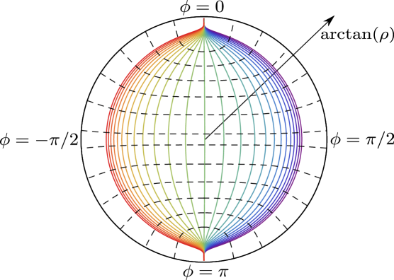
Figure 4: Embedding of the branes given by $y=-y_{*}$ in AdS space with coordinates $t,\rho,\phi$. The spacetime to the right of each of these curves corresponds to the region $N_{+}$ in figure 2, while the part of the spacetime to their left is excised. We set $t=const.$ to consider a spacelike slice with coordinates $\rho,\phi$, and compactify by plotting $\arctan(\rho)$ as radial coordinate, such that the thick black circle represents the AdS boundary. $\phi$ is the angular coordinate. The values of $\lambda$ for the branes shown are specified by $y_{*}=\text{arctanh}(\frac{\kappa\lambda}{2})=\{-3,-2.75,...,3\}$. Lines involving red colour (bending to the left) stand for branes with $\lambda>0$, while lines involving blue colour (bending to the right) stand for branes with $\lambda<0$. The straight vertical line is the brane with zero tension, $\lambda=0$. The black dashed lines are geodesics perpendicular to the branes, see section 6.3.

Let us now discuss the geometries obtained by this construction. For $\lambda=0=y_{*}$, i.e. the case without tension, we just cut the AdS space in half and match the two sides (i.e. $N_{-}$ and $N_{+}$, see figure 2) trivially. For general values of $\lambda$, the profile of the brane $y=-y_{*}$ with respect to $N_{+}$ is shown in figure 4. $N_{+}$ in this figure is always to the right side of the brane. As we can see, for $\lambda>0$ the branes extend to the left, such that $N_{+}$ is larger than half of the AdS space, while for $\lambda<0$ (and hence WEC violation) the branes extend to the right, hence making $N_{+}$ smaller than half of the AdS space, see also figure 5.

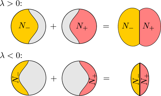
Figure 5: Nontrivial matching of two AdS spacetimes along a constant tension brane for the cases $\lambda>0$ and $\lambda<0$. The two figures to the left of the equality depict the embedding of the brane with respect to $N_{-}$ and $N_{+}$, respectively. The grey shaded area is then excised, and the two resulting spacetimes are glued together along the brane, as shown to the right of the equality. By assumption of symmetry, $N_{-}$ is always the mirror image of $N_{+}$. As described in the text, the resulting spacetime will have increased volume for $\lambda>0$ and smaller volume than $\text{AdS}_{3}$ for $\lambda<0$.

6.3 Normal geodesics

As seen in the previous section, the branes parameterised by their tension $\lambda$ are described by an embedding of the form $y=-y_{*}(\lambda)$. Obviously, the curves $x^{\mu}(y)=\left(t_{0},r_{0},y\right)$ are normal to all of these branes as $\dot{x}^{\mu}=n^{\mu}$ with the normal vector $n$ and have the coordinate $y$ as affine parameter. As it turns out, these curves actually describe geodesics, as with this ansatz the geodesic equations $\ddot{x}^{\mu}+\Gamma^{\mu}_{\alpha\beta}\dot{x}^{\alpha}\dot{x}^{\beta}=0$ simplify to $\Gamma^{\mu}_{yy}=0$. From the metric (43) it is indeed easy to see that this is satisfied. Indeed, these geodesics normal to the branes are exactly those which are symmetric to reflections about the brane with vanishing tension, i.e. with $\lambda=0\Rightarrow y_{*}=0$, see figure 4. Hence we know that due to the backreaction of the brane, all these geodesics are extended by an amount of $2y_{*}$ compared to the pure $\text{AdS}_{3}$ case $\lambda=0$. For boundary regions that extend symmetrically to the left and right from the point where the brane meets the boundary, this means that the entanglement entropy increases by an amount of exactly $y_{*}/2G_{N}$. This coincides with the result of Azeyanagi:2007qj . In the next section, we will discuss entanglement entropy for intervals that do not include the point where the brane is anchored at the boundary.

6.4 Entanglement entropy of general intervals

The major motivation to investigate the backreaction on the geometry is that it is necessary for calculating the entanglement entropy using the Ryu-Takayanagi proposal Ryu:2006bv ; Ryu:2006ef . This states that the entanglement entropy of some spacelike area in the field theory is proportional to the area of a spacelike minimal surface in the bulk with the same boundary.

In 2+1 bulk dimensions, the area will be given by a line segment $[AB]\subset M$ on the conformal boundary and the extremal surface by the geodesic connecting the boundaries of $[AB]$ which we denote $\varUpsilon_{[AB]}$. Furthermore $\partial[AB]=\partial\varUpsilon_{[AB]}=\{A,B\}$. The proposal is then given by

$$S_{[AB]}=\frac{\text{min area}(\varUpsilon_{[AB]})}{4G_{N}}.$$ (55)

In the probe limit, the geometry does not change according to the fields on the defect and thus the entanglement entropy cannot be affected since localised energy-momentum does not alter the variational problem for minimal surfaces.

In this section we point out one important difference between the cases of positive and negative brane tension $\lambda$ with respect to the holographic calculation of entanglement entropy. These cases can be physically distinguished by WEC (satisfied for $\lambda\geq 0$, violated for $\lambda<0$) and SEC (violated for $\lambda>0$, satisfied for $\lambda\leq 0$).

First, let us mention that the surface defined by $y=0$ in figure 6 is an extremal surface barrier in the sense of Engelhardt:2013tra and the barrier theorem given in section 5. This means that if we have two points $A$ and $B$ on the boundary (to the same side of the brane), the extremal curve $\varUpsilon_{[AB]}$ connecting the two points in the bulk cannot cross this surface, see figure 6. Note that as we work in $2+1$ bulk dimensions, and as we suppress the (static) time direction, the length of this curve $\varUpsilon_{[AB]}$ determines the entanglement entropy of the interval between $A$ and $B$.

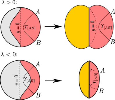
Figure 6: Spacelike geodesics $\varUpsilon[AB]$ defining entanglement entropy for intervals $[AB]$ in the cases $\lambda>0$ and $\lambda<0$. $y=0$ would be the brane for the tensionless case $\lambda=0$. For $\lambda<0$, the geodesics $\varUpsilon[AB]$ may intersect the brane and may be reflected/refracted by it.

For $\lambda>0$, the brane, given by $y=-y_{*}$, stays behind the extremal surface barrier $y=0$ (see figure 6) and is hence itself an extremal surface barrier, just as $Q_{2}$ in figure 3. This means that the new spacetime we obtain has more volume than global $\text{AdS}_{3}$ and geodesics crossing the brane perpendicularly are longer than in the tensionless case, i.e. the entanglement entropy given by these curves increases, see section 6.3. This makes sense if we assume that the interface described by the brane introduces new degrees of freedom into the system. Geodesics which are not crossing the barrier, such as $\varUpsilon_{[AB]}$ in the figure 6, will be unaltered, which means that if we take any boundary interval $[AB]$ such that the brane does not reach the AdS boundary within this interval, its entanglement entropy will be precisely the same as in the pure AdS case.

For $\lambda<0$ in contrast, the brane at $y=-y_{*}$ crosses the extremal surface barrier $y=0$, see figure 6. This means that the new spacetime we obtain by excising the grey area has less volume than AdS, and geodesics crossing the brane perpendicularly are shorter than in the tensionless case, i.e. also the entanglement entropy defined by these curves is smaller (see again section 6.3). Even geodesics which are not crossing the barrier $y=0$, such as $\varUpsilon_{[AB]}$ in the figure 6 may be cut off at the brane, hence the entanglement entropies of intervals like $[AB]$ may be described by altered curves. In principle, we expect that there should always be a minimal curve connecting any two points in the spacetime (see however Fischetti:2014uxa for geometries where this is not the case), but for $\lambda<0$ it appears that there exist curves which must be refracted (or reflected) at the brane.

The refraction conditions at the brane follow from a local minimisation problem, see JLM:146195 . However, there is a subtlety: Suppose we would like to connect two points $A$ and $B$ which lie in the interior (or on the conformal boundary) of $N_{+}$ for $\lambda<0$. Moreover, suppose that a segment of the original geodesic connecting the points is excised by our approach as indicated in figure 6. In this case, the curve of minimal length connecting $A$ and $B$ clearly cannot lie only in the interior of $N_{+}$, since there the geometry is smooth and there is always a mean curvature flow which leads towards the original geodesic and hence the brane. If the geodesic approaches the brane at a finite angle, then due to the refraction conditions (which are given by a generalised Snell’s law, see JLM:146195 ) it would continue in $N_{-}$ with a finite angle, too. In order to return to $N_{+}$ it must cross the brane at least once more. However, the segment connecting both crossing points, regarded as elements of $N_{-}$, cannot be of minimal length for negative tension. In the original spacetime, the geodesic connecting those points would lie entirely in the excised part. The same argument holds for curves connecting the crossing points (now regarded as elements of $N_{+}$) and lying in the interior of $N_{+}$. Hence the minimal curve connecting the “crossing” points must lie on the brane. Thus we can reduce the problem to considering minimal curves lying in $N_{+}\cup Q$ only.

Now that a finite segment of the minimal curve connecting $A$ and $B$ lies completely on the brane, the curve is not allowed to reach the brane at a finite angle. Otherwise, it would have a kink at that point which can always be replaced by a smooth edge of minor length. Thus the desired minimising curve connecting $A$ and $B$ consists of three segments: The first segment is a geodesic in $N_{+}$ connecting $A$ with the entrance point on the brane at which it ends tangentially. The second segment lies entirely on the brane, connects the entrance and exit points and is required to be a geodesic w.r.t. the induced geometry on the brane. The last segment is again a geodesic in $N_{+}$ which leaves the brane tangentially and connects the exit point on the brane and $B$. The discussion is illustrated in figure 7.

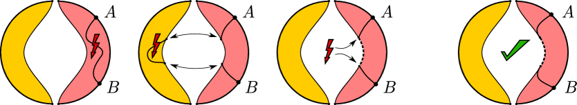
Figure 7: The four possibilities of minimal curves connecting two points $A$ and $B$ for $\lambda<0$ as considered in the main text. The first three possibilities are excluded by general properties of geodesics in AdS if a part of the original geodesic is excised by the approach. The only possibility left is the forth in which the dashed part of the curve is not geodesic w.r.t. to the ambient geometry, but nevertheless minimal.

To summarise, for $\lambda<0$ we obtain that the holographic entanglement entropy of intervals which do not include the defect itself becomes affected. When tuning $\lambda$ from $0$ to $-\frac{1}{4\pi G_{N}}$, the first geodesics to intersect the brane are those reaching deep into the bulk and hence belonging to large intervals $[AB]$. The geodesics belonging to smaller intervals $[AB]$ will intersect the brane for smaller values of $\lambda$. Due to this behaviour, it would be very interesting to find systems in which $\lambda<0$ is satisfied and study the impact of what was found above, see also the discussion in section 9.

7 Perfect fluid on the brane

Let us now come to one of the main results in this paper. Using the decomposition of the equations (12) into scalar equations outlined in section 4.1, it is possible to find simple analytical expressions for the (static) embedding of the brane $Q$ in the case where the matter content on $Q$ is a perfect fluid. We compute the brane embeddings explicitly for this case.

7.1 Perfect fluid in Poincaré AdS

Let us consider the configuration where the brane matter is given by a perfect fluid. The brane is embedded in a Poincaré AdS geometry, hence $h(z)=1$ and $h^{\prime}(z)=0$ in (8). To keep track of the AdS-scale $L$, we assume

$$x_{+}(z)\rightarrow L\cdot x_{+}\left(\frac{z}{L}\right)$$ (56)

so that $x_{+}$ is a dimensionless function with a dimensionless argument, and find for the extrinsic curvature scalars defined in (32) and (34)

$$\mathcal{K}_{L/R} =\frac{zx_{+}^{\prime\prime}(z/L)}{2L^{2}(1+x_{+}^{\prime}(z/L)^{2})^{3/2}},$$ (57)

$$\mathcal{K} =\frac{2Lx_{+}^{\prime}(z/L)^{3}+2Lx_{+}^{\prime}(z/L)-zx_{+}^{\prime\prime}(z/L)}{L^{2}(1+x_{+}^{\prime}(z/L)^{2})^{3/2}}.$$ (58)

As we assume the matter content on the brane to be a perfect fluid, the energy-momentum tensor is given by

$$S_{ij}=(\rho+p)u_{i}u_{j}+p\gamma_{ij}$$ (59)

with $u_{i}\sim(1,0)$ for staticity, which easily gives

$$S =p-\rho,\ \ S_{L/R}=\frac{p+\rho}{2}.$$ (60)

Let us now assume an equation of state

$$p=a\cdot\rho$$ (61)

with constant $a$ so that

$$S =\rho(a-1),\ \ S_{L/R}=\rho\frac{1+a}{2}$$ (62)

and the energy conditions, assuming $\rho>0$, read

$$\text{NEC:\ \ }a\geq-1,\ \ \text{WEC:\ \ }a\geq-1,\ \ \text{SEC:\ \ }a\geq 0.$$ (63)

There are now two possible ways to proceed towards exact solutions of this system. The first one is to take the two scalar equations (34) and get rid of $\rho(z)$ by setting up the equation

$$\frac{\mathcal{K}}{\mathcal{K}_{L/R}}=\frac{2(a-1)}{a+1}=const.$$ (64)

which is then a first order ODE for $x_{+}^{\prime}(z/L)$ and can be easily solved by separation of variables.

The second, more easily generalisable method is to make use of equation (37) which for the perfect fluid under consideration here reads

$$\rho(z)^{\prime}=\frac{1+a}{a}\frac{\rho(z)}{z}\ \ \Rightarrow\ \ \rho(z)=\frac{2c}{\kappa L}\left(\frac{z}{L}\right)^{1+\frac{1}{a}},$$ (65)

with $c$ some positive number of our choice. Inserting this into (34) and solving for the profile $x_{+}(z)$, we find (with $y\equiv z/L$),

$$x_{+}^{\prime}(y) =\frac{acy^{\frac{1}{2}\left(2+\frac{2}{a}\right)}}{\sqrt{1-a^{2}c^{2}y^{2+\frac{2}{a}}}},$$ (66)

$$x_{+}(y) =\frac{a^{2}cy^{2+\frac{1}{a}}{}_{2}F_{1}\left(\frac{1}{2},\frac{1+2a}{2+2a};\frac{3+4a}{2+2a};a^{2}c^{2}y^{2+\frac{2}{a}}\right)}{1+2a},$$ (67)

with ${}_{2}F_{1}(a,b;c;d)$ the hypergeometric function. It may be shown that as $y\rightarrow\left(\frac{1}{a^{2}c^{2}}\right)^{\frac{a}{2a+2}}$, the derivative diverges while the function itself reaches a finite value. Also, the function is real only for $y\leq\left(\frac{1}{a^{2}c^{2}}\right)^{\frac{a}{2a+2}}$ and below, i.e. at the critical value and closer to the boundary, for $a\geq 0$ (i.e. SEC) and $a\leq-1$. For the intermediate range $-1<a<0$, we do not obtain solutions for which the brane actually reaches the boundary, and therefore we will ignore this parameter range. While the SEC may easily be violated by sensible classical matter (see section 8), we assume NEC to be satisfied (see the discussion at the end of section 4.2) and hence we will in the following only discuss the solutions for $a\geq 0$. See figure 8 for plots of the embedding function $x_{+}$ for several values of the parameters.

At the critical value of $y$ where the derivative of $x_{+}$ diverges, the brane should not simply end, but instead be joined with a similar profile that symmetrically goes back to the boundary. So the brane starts at the boundary and enters the bulk, until at some critical value of $y$ it turns around and returns to the boundary in a symmetric fashion. This is interesting, since it means that a finite part of the boundary is enclosed by the brane and hence by gluing two parts together the spatial boundary of the spacetime is compactified. The final result is of the form discussed in section 6, see in particular the right hand sides of figures 5 and 6.

Will the perfect fluid rather resemble the $\lambda>0$ or the $\lambda<0$ case of the discussion in 6? As discussed above, for $a\geq 0$ the perfect fluid satisfies both WEC and SEC. Due to the barrier theorem (see the discussion in section 5), we know that extremal curves anchored to one side of the brane will not cross it and hence cannot be altered by it. For spacelike codimension one extremal surfaces describing entanglement entropy, this can be seen easily from figure 8: In AdS space the geodesics are half circles, and it can be shown that any half-circle anchored to the boundary on one side of the brane will never intersect this brane. This is because the brane always extends further into the bulk than the largest half-circle that could possibly be anchored on one side of the brane, compare $\varUpsilon_{2}$ and $Q_{1}$ on the left side of figure 3. In fact, in the limit $a\rightarrow+\infty$ the profile (67) asymptotes to the half circle drawn as $\varUpsilon_{2}$ in figure 3.

Figure 8: Left: Brane profiles (67) (added with symmetric parts leading back to the boundary) for $L=1,c=1/a$ and, in order of increasing second intersection with the $x$-axis, $a\approx 0.1,0.2,0.4,0.7,1.1,2.0,4.8,100$. Right: Brane profiles with $L=1,a=1$ and, from outer to inner curve, $c=0.5,1,1.5,...,5$. Note that all the turning points lie on a straight line, indicated in dashed black.

7.2 Perfect fluid in AdS with cosmological constant

The results obtained above may be generalised to the case where the tension on the brane involves a cosmological constant. Generalising (62), let us now assume

$$S =\Omega+\rho(a-1),\ \ S_{L/R}=\rho\frac{1+a}{2},$$ (68)

which corresponds to a cosmological constant (or equivalently a constant tension) $\Omega$ on the brane. This leads to a situation where the SEC is violated at least near the boundary, and may or may not become satisfied deeper in the bulk, depending on the energy content of the perfect fluid. This situation is interesting in the light of the discussion given in section 5: Will the branes generally turn around and bend back to the boundary?

$\Omega$ drops out of the equation (37) when differentiating, so we end up with the same solution for $\rho$ as before: $\rho(z)=cz^{1+\frac{1}{a}}$ where we set $L=1$ and $\kappa=2$ for simplicity. By the scalar equations of motion (34) we now find

$$\Omega+2a\rho(z)=\mathcal{K}+2\mathcal{K}_{L/R}=\frac{2x_{+}^{\prime}(z)}{\sqrt{1+x_{+}^{\prime}(z)^{2}}}$$ (69)

and integrate with the result

$$x_{+}^{\prime}(z) =\frac{\Omega+2a\rho}{\sqrt{4-(\Omega+2a\rho)^{2}}}$$ (70)

$$\Rightarrow x_{+}(z) =\frac{z}{(1+2a)\sqrt{4-\Omega^{2}}}$$ (71)

$$\times\Bigg{[}(\Omega+2a\Omega)F_{1}\left(\frac{a}{1+a};\frac{1}{2},\frac{1}{2};\frac{1+2a}{1+a};-\frac{2acz^{1+\frac{1}{a}}}{-2+\Omega},-\frac{2acz^{1+\frac{1}{a}}}{2+\Omega}\right)$$

$$+2a^{2}cz^{1+\frac{1}{a}}F_{1}\left(\frac{2+a}{1+a};\frac{1}{2},\frac{1}{2};\frac{3+2a}{1+a};-\frac{2acz^{1+\frac{1}{a}}}{-2+\Omega},-\frac{2acz^{1+\frac{1}{a}}}{2+\Omega}\right)\Bigg{]}$$

where $F_{1}(a;b,c;d;e,f)$ is the Appell hypergeometric function.

As expected, the behaviour is dominated by the cosmological constant near the boundary and by the perfect fluid in the bulk, see figure 9 (left). This also means that these branes do in fact bend back to the boundary.

Let us briefly mention that in the limit $c\rightarrow 0$, the above results show us that for a constant tension and no other matter-energy content on the brane in Poincaré AdS the solution simply reads:

$$x_{+}(z)=\frac{\Omega z}{\sqrt{4-\Omega^{2}}},$$ (72)

i.e. the brane is defined by a straight line in Poincaré coordinates as was found before Takayanagi:2011zk ; Fujita:2011fp ; Nozaki:2012qd .

7.3 Perfect fluid in BTZ

Let us repeat the calculation of section 7.2 in the BTZ background (8), still assuming $L=1,\ \kappa=2$ and (68). The solution to (38) now reads

$$\rho(z)=c\left(\frac{z^{2}z_{H}^{2}}{z_{H}^{2}-z^{2}}\right)^{\frac{a+1}{2a}}.$$ (73)

From the equations (34) we find again:

$$\Omega+2a\rho(z)=S+2S_{L/R}=\frac{2z_{H}x^{\prime}_{+}(z)}{\sqrt{(z_{H}^{2}-z^{2})x_{+}^{\prime}(z)^{2}+z_{H}^{2}}}.$$ (74)

Obviously, together with (73) this can be solved to give an analytic expression for $x^{\prime}_{+}(z)$, yet unfortunately this expression cannot be integrated to a closed form expression for $x_{+}(z)$ for general parameters $\Omega,a,c,z_{H}$. In any case, by investigating the limit $z\rightarrow 0$ we see that, assuming $a>0$, $x^{\prime}_{+}(z)$ and hence $x_{+}(z)$ are real for small enough $z$ whenever $\Omega^{2}<4$, as expected. Also assuming $a>0,\Omega^{2}<4$, it may be shown that $x^{\prime}_{+}(z)$ necessarily diverges for some finite value $z_{crit}<z_{H}$, i.e. the brane will always bend back to the boundary before reaching the event horizon, see figure 9 (right).

Figure 9: Left: Embedding functions (71) (with additional symmetric branches leading back to the boundary) for $L=1$, $a=c=1$ and, in order of increasing second intersection with the $x$-axis, $\Omega=-1,-0.5,0,0.5,1$. Right: Embedding functions for the brane with a perfect fluid in a BTZ background. Depicted are the cases for $\Omega=0$, $L=a=c=1$ and, in order of increasing second intersection with the $x$-axis, $z_{H}=0.5,1,1.5,...,3$.

7.4 Relation to scalar field

A perfect fluid with an equation of state (61) may not seem to be a model of matter that might appear in a ‘fundamental’ holographic construction of a given DCFT or BCFT. Nevertheless, we would like to point out that at least in the static case the conformal fluid with $a=1$ may be shown to be equivalent to a free massless scalar field with action

$$\mathcal{L}_{matter,\,Q}=-\frac{1}{2}\gamma^{ij}\partial_{i}\phi\partial_{j}\phi.$$ (75)

Specifically, identifying $\rho\equiv\frac{1}{2}\gamma^{ij}\partial_{i}\phi\partial_{j}\phi=\frac{\gamma^{zz}}{2}\left(\phi^{\prime}\right)^{2}$, the equations of motion

$$\gamma^{\prime 11}\phi^{\prime}-\frac{2}{z}\gamma^{11}\phi^{\prime}+2\gamma^{11}\phi^{\prime\prime}=0$$ (76)

following from (75) take precisely the form (65) for a Poincaré background and we also recover (62). In this way, the solutions presented in the previous subsections for $a=1$ can equally be interpreted as solutions for the massless free scalar field.

We conclude with a short summary of what was derived in this section. We found explicit analytic solutions for the backreaction in the AdS/BCFT ansatz as described in sections 2 and 3. In particular, we found solutions for the case when the energy-momentum tensor on the brane is described by a perfect fluid. Moreover, we also considered the case where we add a constant brane tension to a perfect fluid in an ambient AdS or BTZ background in 2+1 dimensions. For all of these cases, due to the barrier theorem the brane has to bend back to the boundary and hence the spatial boundary direction has to be compactified. It will also be interesting to make contact between the present results for $a=1$ and the discussion of holographic boundary RG flows as considered in Nakayama:2012ed .

8 A holographic model of the Kondo effect

In this last section, we focus on a particular holographic model, namely the holographic Kondo model proposed in Erdmenger:2013dpa (see e.g. 2001cond.mat..4100K for a review of the Kondo model in field theory). This describes the coupling of an impurity in a 1+1-dimensional CFT, i.e. in a DCFT. Hence we assume that the formalism described in section 3 is applicable. In Erdmenger:2013dpa , the probe limit was considered in which the brane is fixed to be given by a totally geodesic brane embedding $x_{\pm}=0$, and the energy-momentum tensor of the brane does not backreact to the geometry.

As mentioned before, the probe limit cannot give information about the behaviour of entanglement entropy near the defect as it is fixed by the ambient geometry, at least for the Ryu-Takayanagi formalism Ryu:2006bv ; Ryu:2006ef . Here, we shed some light on this topic by including the backreaction for the dual Kondo system.

In sections 4 and 5 we saw how critical it is for the structure of the embedding whether certain energy conditions are satisfied or violated. In section 7 we studied a concrete example of an energy-momentum tensor on the brane that everywhere satisfies WEC and SEC. By the results in table 1, SEC implies that initially $x^{\prime}_{+}\geq 0$, i.e. the brane profile $x_{+}$ initially bends to the right in figure 2. Then, by WEC, SEC and the theorem presented in section 5, the brane has to reach back to the boundary after a finite distance $\Delta x$. This especially means that in 2+1 dimensions, with an ansatz relying on matter fields on the brane that satisfy WEC and SEC, it will not be possible to find a solution where the brane falls into the event horizon of a black hole, as for example in Magan:2014dwa . If this was the case for all physical models, it would be very restrictive from the point of view of model building.

Hence, in this section we will present a physically motivated ansatz for matter fields living on the brane that leads to a SEC violation, and brane embedding solutions that do indeed reach into a black hole event horizon. The matter content on the brane is given by a scalar field charged under a $U(1)$ gauge field, which as well is contrained to the brane, and a $U(1)$ Chern-Simons field, which is defined throughout the bulk.

The matter fields on the brane are assumed to be given by the action

$$\mathcal{S}=-\mathcal{N}\int\text{d}^{2}x\,\sqrt{-\gamma}\,\left(\frac{1}{4}f_{mn}f^{mn}+\gamma^{mn}(D_{m}\Phi)^{\dagger}(D_{n}\Phi)+V(\Phi\Phi^{\dagger})\right),$$ (77)

where $\mathcal{N}$ is a factor which may be fixed in a top-down string theory derivation of the model, see for instance Erdmenger:2013dpa . $D$ denotes gauge covariant differentiation w.r.t. the gauge field $a$ and the Chern-Simons field $A$, given by

$$D_{m}\Phi\equiv\partial_{m}\Phi+i\,A_{m}\Phi-i\,a_{m}\Phi.$$ (78)

For simplicity, we will henceforth set the bulk Chern-Simons field to zero, $A=0$, as it would otherwise contribute to the equations of motion with its own junction conditions. We will investigate the solutions of the full system (including the Chern-Simons field) and their interpretation as a model of the Kondo effect in a forthcoming publication Erdmenger:2015spo .

8.1 A gauge field on the brane

Let us first only look on the case of a $U(1)$-field on the brane with $\Phi\equiv 0$ which resembles the background solution of the Kondo model in the normal phase. The energy-momentum tensor for the gauge field reads

$$S^{(a)}_{ij}=-\frac{\mathcal{N}}{4}f^{mn}f_{mn}\gamma_{ij}+\mathcal{N}\gamma^{mn}f_{mi}f_{nj}$$ (79)

which can be decomposed into a trace part

$$S^{(a)}=\frac{\mathcal{N}}{2}f^{mn}f_{mn}$$ (80)

and a traceless part given by

$$S^{(a)}_{ij}-\frac{S^{(a)}}{2}\gamma_{ij}=-\frac{\mathcal{N}}{2}f^{mn}f_{mn}\gamma_{ij}+\mathcal{N}\gamma^{mn}f_{mi}f_{nj}.$$ (81)

The equations of motion in the absence of currents

$$\partial_{m}\left(\sqrt{-\gamma}\gamma^{mp}\gamma^{nq}f_{pq}\right)=0$$ (82)

imply due to antisymmetry $\sqrt{-\gamma}f^{01}=:C$, with $C$ constant. This is the electric flux due to the gauge field.

We will now assume a static configuration which means, as we saw in section 4.3, that the metric takes the form (25). As the tensor $f_{mn}$ is antisymmetric and hence has only one component that can be specified in 1+1-dimensions, it is straightforward to show $f^{mn}f_{mn}=-2C^{2}$ and $\gamma^{mn}f_{mi}f_{nj}=-\gamma_{ij}C^{2}$. This means that the traceless part (81) vanishes identically, and the energy-momentum tensor takes the form

$$S^{(a)}_{ij}=-\frac{\mathcal{N}}{2}\gamma_{ij}C^{2}$$ (83)

which corresponds to a (WEC satisfying, SEC violating) constant tension $\lambda=\mathcal{N}C^{2}/2$.

Motivated by the results in Azeyanagi:2007qj (see our section 6) in which the authors obtained that the final embedding can be reached via a geodesic normal flow, we now investigate whether this can be generalised to other spacetimes as well. The construction is then as follows, see figure 10: Starting from the trivial embedding $x_{+}=0$, we follow the geodesics starting normal to the hypersurface for a certain arclength $s$, depicted by the solid black lines. The arclength $s$ can be matched to the brane tension $\lambda$ using (54), in which we have to identify $y_{\ast}$ with $s$ such that

$$\tanh(s/L)=\frac{L}{2}\kappa\lambda=\frac{L}{4}\kappa\mathcal{N}C^{2}.$$ (84)

This relationship remains valid for our case with a BTZ background and even more general spacetimes, see appendix B. Note that (84) yields a bound on the energy momentum tensor on the brane. In particular, for our matter content it reads

$$|L\kappa\mathcal{N}C^{2}|<4.$$ (85)

For the limiting case, $s\rightarrow\infty$, the embedding of $Q$ is given by the conformal boundary and the construction considered is no longer applicable.

Figure 10: Construction of constant brane tension solutions in a BTZ geometry using a geodesic normal flow. We start from the trivial, totally geodesic embedding $x_{+}=0$ (for which $s=0$) and follow the flow generated by geodesics normal to the trivial embedding and pointing outward of $N_{+}$. The region to the left of the family of embeddings is excluded from $N_{+}$. The dashed lines to the right hand side denote the continuation of the generating geodesics.

The family of embeddings $X_{s}:Q\hookrightarrow N_{+}$ is explicitly given by

$$X_{s}(t,z_{b})=(t,x_{+}(z_{b}),z(z_{b}))=\left(t,-z_{H}\,\text{arctanh}\left(\frac{z_{b}}{z_{H}}\tanh(\frac{s}{L})\right),\frac{z_{b}}{\sqrt{1+f(z_{b})\sinh^{2}(\frac{s}{L})}}\right)$$ (86)

with $(t,z_{b})$ the point at which the geodesics start on the trivial embedding. The induced metric and the extrinsic curvature are computed to be

$$\gamma_{s}=f_{s}^{\,\ast}g=\left(\frac{L\cosh(s/L)}{z_{b}}\right)^{2}\left(-f(z_{b})\,\text{d}t^{2}+f^{-1}(z_{b})\,\text{d}z_{b}^{2}\right)$$ (87)

$$K_{s}=\frac{-L\sinh(s/L)\cosh(s/L)}{z_{b}^{2}}\left(-f(z_{b})\,\text{d}t^{2}+f^{-1}(z_{b})\,\text{d}z_{b}^{2}\right).$$ (88)

Note that the normal flow changes the induced metric only by a conformal factor. Furthermore, the extrinsic curvature is proportional to the induced metric

$$K_{s}=\frac{-\tanh(s/L)}{L}\gamma_{s}$$ (89)

and for $s=0$ we recover the trivial embedding. This proportionality is necessary to satisfy the Isreal junction conditions for constant tensions, see also appendix B.

To obtain explicit solutions in a BTZ background, we can choose the gauge $a_{z}=0$ and integrate $\partial_{z}a_{t}=\sqrt{-\gamma}C$ with boundary condition $a_{t}(z_{H})=0$ for regularity. Moreover we may solve (86) for $x_{+}$ as a function of $z$ for constant $s$. We obtain

$$a_{t}=\int\limits^{z}_{z_{H}}\sqrt{-\gamma}\,C =\frac{CL^{2}}{z_{H}}\cosh(s/L)\left(\cosh(s/L)-\sqrt{(z_{H}/z)^{2}+\sinh^{2}(s/L)}\right)$$ (90)

$$x_{+}(z) =-z_{H}\,\text{arctanh}\left(\frac{\sinh(s/L)}{\sqrt{(z_{H}/z)^{2}+\sinh^{2}(s/L)}}\right)$$

where the arclength $s$ and the electric flux $C$ still have to be matched according to (84) in order to satisfy the equations of motion.

8.2 A gauge field with non-trivial scalar on the brane

Now that we found the background solutions (90), we allow the scalar field in (77) to be non-vanishing. In the holographic Kondo model, this amounts to an RG flow triggered by a marginally relevant operator, and to a phase transition to the condensed phase in the large $N$ limit Erdmenger:2013dpa . This corresponds to the formation of the Kondo screening cloud. Upon turning on the scalar field we have to add the scalar sector of the energy-momentum tensor to (79), which reads

$$S^{(\Phi)}_{ij}=2\mathcal{N}\left[(D_{(i}\Phi)^{\dagger}D_{j)}\Phi-\frac{1}{2}\gamma_{ij}\left(|D\Phi|^{2}+V(\Phi^{\dagger}\Phi)\right)\right].$$ (91)

The total energy-momentum tensor is hence given by

$$S^{(tot)}_{ij}=S^{(a)}_{ij}+S^{(\Phi)}_{ij}.$$ (92)

For the static case in two dimensions the scalar part may be decomposed as

$$S^{(\Phi)}=-2\mathcal{N}V(\Phi^{\dagger}\Phi),\ \ S^{(\Phi)}_{L/R}=\frac{\mathcal{N}}{2}\tilde{\gamma}^{ij}(D_{i}\Phi)^{\dagger}D_{j}\Phi,$$ (93)

$\tilde{\gamma}_{ij}$ being defined in (29). As the latter is manifestly positive, we see that the scalar field always satisfies NEC.

To apply the results of section 5, we need to make statements about the violation of WEC and/or SEC as well. For the holographic Kondo model, we find that in contrast to the perfect fluid solutions discussed in section 7, the SEC is violated everywhere on the brane. This can easily be seen from the numerical solutions in figure 11, since here $x^{\prime}<0$ between the conformal boundary and the event horizon. Due to the results of table 1, this corresponds to SEC violation.

The equations of motion for the scalar $\Phi$, the gauge field $a_{t}$ (we gauge $a_{z}=0$) and the embedding scalar $x_{+}$ read

$$\gamma^{\alpha\beta}\mathfrak{D}_{\alpha}\mathfrak{D}_{\beta}\Phi-M^{2}\Phi =0,$$ (94)

$$\partial_{z}\sqrt{-\gamma}f^{zt}+J^{t} =0,$$ (95)

$$\mathcal{K}_{zz}-\frac{\kappa}{2}S^{(tot)}_{zz} =0,$$ (96)

where we defined the gauge covariant derivative $\mathfrak{D}=\nabla+ia$ with $\nabla$ the induced connection on the brane and the conserved current $J^{\mu}=-2\sqrt{-\gamma}\gamma^{\mu\nu}(a_{\nu})\Phi^{2}$. Regularity at the event horizon requires

$$\Phi^{\prime}(z_{H})=-\frac{L^{2}\,M^{2}\Phi(z_{H})}{2z_{H}},\qquad a_{t}(z_{H})=0,\qquad x_{+}^{\prime}(z_{H})=\kappa\,\frac{2L^{4}M^{2}\Phi(z_{H})^{2}-z_{H}^{\,4}\,a_{t}^{\prime}(z_{H})^{2}}{4L^{3}},$$ (97)

which fixes half of the integration constants. Since the embedding enters the EOMs only via its first and second derivative, its remaining integration constant can easily be fixed by requiring $x_{\pm}(0)=0$. This is resonable since the ambient spacetime is invariant under translations in $x$-direction.

We start by treating the scalar field as a probe w.r.t. the background solution (90). The leading order behaviour of the gauge field reads

$$a_{t}\sim\frac{-CL^{2}\cosh(s/L)}{z}+\frac{CL^{2}\cosh^{2}(s/L)}{z_{H}}+\ldots=:Q/z+\mu_{c}+\ldots$$ (98)

where we defined $Q=-CL^{2}\cosh(s/L)$ and $\mu_{c}=CL^{2}\cosh^{2}(s/L)/z_{H}$, the latter being identified with the chemical potential for the $U(1)$ charge. If the scalar is nonzero, we have $\mu>\mu_{c}$. Furthermore, from (84) we obtain $L\kappa C^{2}=4\tanh(s/L)$ and hence a restriction on the magnitude of $C$ as mentioned above.

Turning on the scalar near the boundary, we find that there are two asymptotic solutions which read

$$\Phi\sim z^{p},\qquad p=\frac{1}{2}\left(1\pm\sqrt{1+4(L^{2}M^{2}-Q^{2})\cosh^{2}(s/L)}\right).$$ (99)

To obtain the correct operator dimensions for mapping our bottom-up model to the Kondo effect, just as in Erdmenger:2013dpa we need $p=1/2$. This means that our scalar field saturates the Breitenlohner-Freedman bound and we have to adjust the mass of the scalar to be given by

$$M^{2}=\frac{4Q^{2}\cosh^{2}\left(s/L\right)-1}{4L^{2}\,\cosh^{2}\left(s/L\right)}=\left(\frac{Q}{L}\right)^{2}-(4L^{2}\,\cosh^{2}\left(s/L\right))^{-1}.$$ (100)

The asymptotic behaviour of the scalar is then given by

$$\Phi(z)\sim\alpha\sqrt{z}\log(z\Lambda)+\beta\sqrt{z}+\ldots$$ (101)

where we introduced an arbitrary energy scale $\Lambda$ to define the logarithm. It was shown in Erdmenger:2013dpa that switching on the scalar triggers the running of the Kondo coupling. The dual operator is similar to the double trace operator considered in Witten:2001ua . Thus the Kondo coupling is given by $\kappa=\alpha/\beta$.

The leading order coefficient $\alpha$ is proportional to the vacuum expectation value of the dual operator on the field theory side,

$$\alpha\sim\langle\mathcal{O}\rangle,$$ (102)

such that a non-vanishing scalar field leads to the condensation of the Kondo singlet in the field theory. For further details we refer the reader to Erdmenger:2013dpa .

Now fixing $L$, $z_{H}$, $\kappa$ and $C$ we solve for $Q$, $M^{2}$ and $s$ by using the formulae above. We may turn on the scalar field by either increasing the chemical potential $\mu$ or the leading order coefficient $\alpha$ of the scalar. Both approaches are equivalent for our considerations. The phase transition occurs at $\mu=\mu_{c}$, which in the limit $\kappa\rightarrow 0$ (and $s\rightarrow 0$) yields the value for the probe solution $\mu=-Q$. Note that the critical value for the chemical potential diverges if we saturate the bound (85) discussed above.

To solve the system of ODEs (94)-(96), we apply the finite difference method. We fix $L=1$, $\kappa=1$, $C=1/2$ and $z_{H}=1$ for concreteness. To have control on the steep behaviour of the fields near the boundary, we subdivided the radial direction $z\in(0,1)$ into two subregions $z_{L}=(0,0.1)$ and $z_{R}=(0.1,1)$. In $z_{L}$, the ODEs were discretised on an evenly spaced grid with 300 points while in $z_{R}$, we applied a Chebyshev grid with 50 points.

Results for the embedding scalar $x_{+}(z)$ for different values of $\alpha\sim\langle\mathcal{O}\rangle$ are shown in figure 11. We see that turning on the scalar field decreases the overall volume of the spacetime, in contrast to what happens if we increase the magnitude of the electric flux $C$. At the boundary, the behaviour of the embedding does not change as the scalar field condenses. Its derivative at the boundary $x_{+}^{\prime}(0)$ is fixed by the asymptotics of the gauge field and thus boundary data, i.e. the brane embedding approaches the conformal boundary tangential to the background embedding.

Figure 11: Numerical solutions for the embedding function $x_{+}(z)$ for different ratios of $\mu/T$. The region between the embedding profile and the $x$-axis is excluded from the spacetime $N_{+}$ as indicated in the plot. The violet curve (thick) is given by a vanishing scalar field $\alpha=0$ and hence (90), where the arclength $s$ has been tuned to be consistent with the gauge field background configuration. The other embeddings are given by numerical solutions for $\alpha=0,0.2,0.4,\ldots,2$ where we set $L=1$, $z_{H}=1$, $C=1/2$ and $\kappa=1$. Increasing $\alpha$ is equivalent to increasing the ratio of $\mu/T$, hence the overall volume of the spacetime decreases as the system undergoes a phase transition from the normal to the condensed phase in the large $N$ limit. The condensed phase corresponds to the formation of the Kondo screening cloud.

8.3 Summary

To summarise, we have found analytic solutions for the brane embedding and the matter field configurations in equilibrium for the case of vanishing scalar field on the brane. In that case, the energy-momentum tensor is given by a constant brane tension and we may construct the embedding by following a geodesic normal flow.

For constant brane tension solutions, the entanglement entropy of symmetric patches around the defect will only differ from that of the trivial solution by a constant offset since due to the refraction conditions at the brane, the generating geodesics are part of the extremal surfaces (dashed lines in figure 10) used in the Ryu-Takayanagi formalism.

Turning on the scalar field decrases the volume of $N_{+}$ and the energy momentum tensor is not given by a constant tension anymore. This can be seen from (93), which implies $S_{L/R}\neq 0$ for a non-vanishing scalar. Hence, the corresponding brane embedding cannot be constructed by a geodesic flow, which means especially that the entanglement entropy of symmetric patches around the defect will be a function of the boundary separation. Renormalising this function by subtracting the normal phase solution with $\Phi=0$ will yield a non-constant function from which we can extract essential information about the Kondo screening cloud and the associated defect entropy. This will be investigated in more detail in Erdmenger:2015spo .

The Kondo model realises a boundary RG flow in agreement with the holographic $g$-theorem. This theorem states that the boundary entropy $S_{bnd}$ decreases along the RG flow Affleck:1991tk ; Friedan:2003yc . From the holographic point of view, this can be derived by requiring the NEC in the bulk and on the brane Takayanagi:2011zk ; Fujita:2011fp . In Takayanagi:2011zk ; Fujita:2011fp , a $g$-function of the form

$$\log(g)\sim-\text{arcsinh}\left(\frac{x_{+}(z)}{z}\right)$$ (103)

was suggested to give the correct answer for the boundary entropy in AdS. We may apply this function to our example as well, since due to the SEC violation, NEC implies $x^{\prime\prime}>0$ in a BTZ background (see table 1). This is essential to prove that this function decreases monotonically along the RG flow.

9 Conclusions and outlook

Motivated by a recent holographic Kondo model Erdmenger:2013dpa , we have studied gravity configurations with matter fields restricted to infinitely thin co-dimension one hypersurfaces, i.e. branes. These configurations are described by equations of motion that involve the extrinsic curvature of these hypersurfaces, as used in the AdS/BCFT correspondence.

In section 3, we considered the gravity dual of a DCFT, where the equations of motion of the brane $Q$ are the Israel junction conditions. This setup may be considered to describe an infinitely thin brane or to describe an approximation to a finitely thin matter configuration. Moreover, we studied the ensuing equations of motion for non-trivial matter fields living on $Q$, both by general arguments and by considering concrete examples.

Section 4 was devoted to decomposing the Israel junction conditions into its trace and off-trace parts, and to a study of the restrictions that energy conditions may impose on the geometry. In section 5, we related these energy conditions to a geometrical theorem, the ‘barrier theorem’, recently obtained by Engelhardt and Wall. Moreover, we deduced qualitative statements on the form that a brane $Q$ may take, depending on whether certain energy conditions are satisfied or violated by the matter fields living on it. We found that if the weak and strong energy conditions are satisfied, the brane has to bend back to the boundary. If just the null energy condition is satisfied, the brane may reach infinitely far into the radial direction of the dual space.

In section 6, we discussed how the well-known toy model of a brane with constant tension arises in our context. Then, in section 7, we found explicit results for the backreacted configurations corresponding to branes whose matter content is given by a perfect fluid, or - equivalently, as we showed - by massless free scalar fields restricted to them. Section 8 was then devoted to the numerical study of a brane with a matter content that appears in the holographic Kondo model of Erdmenger:2013dpa . Due to its violation of the strong energy condition, it reaches all the way to the BTZ horizon in the radial direction and thus shows a qualitatively different behaviour than the bending solutions studied in section 7.

Finally, let us give an outline to the three appendices included below. We comment on the generalisation of the findings of section 5 to special geometries in higher dimensions in appendix A. In appendix B, we justify the geodesic normal flow construction of constant brane tension solutions in sections 6 and 8, and state under which conditions this may be extended to more general setups.

We conclude this work with an outlook on interesting topics that in our eyes warrant further investigation:

The Kondo model: The first issue is of course the holographic model of the Kondo effect Erdmenger:2013dpa . We presented preliminary results for the brane embedding in the backreacted case in section 8. However, further important questions were left unanswered, for example calculating the entanglement entropy for these solutions. Moreover, the behaviour of the field theory dual to the backreacted solution remains undetermined. Also, the model proposed in Erdmenger:2013dpa contains a bulk Chern-Simons-field that we set to zero in section 8. In general however, this field requires its own junction conditions. Interestingly, AdS/BCFT like setups with Chern-Simons fields in the bulk were studied before in Fujita:2012fp ; Melnikov:2012tb . Building upon the results of this work, we intend to revisit all of these questions in a future publication Erdmenger:2015spo .

Exact solutions: In section 7 we presented analytical solutions for the case where the matter living on the brane is a perfect fluid with simple equation of state $p=a\rho$. While this may not be a very realistic model in general, we pointed out in section 7.4 that for the choice $a=1$ it describes a massless free scalar on the brane. A further interesting question will be to evaluate the on-shell action and examining the thermodynamic behaviour of these solutions.

Quantum Hall effect: Furthermore, we would like to shortly comment on the AdS/BCFT model of the quantum Hall effect presented in Melnikov:2012tb . There (see especially figure 2(d) of Melnikov:2012tb ), it was argued that a realistic model of the quantum Hall effect would likely include a brane that is anchored to the boundary twice similar to $Q_{1}$ in figure 3. From our results in section 5, it is now clear that in $2+1$-dimensions the brane can be forced to show such a behaviour by choosing its matter content to satisfy both weak and strong energy condition everywhere. However, the Hall model of Melnikov:2012tb naturally lives in $3+1$-bulk dimensions, so it would be desirable to generalise the findings from section 5 to higher dimensions. We will shortly comment on this in appendix A.

Holographic bilayers: We note that bending brane configurations similar to those we considered in section 7 also appear in recent holographic studies of bilayers Evans:2013jma ; Evans:2014mva ; Grignani:2014vaa . Those studies were performed in top-down probe models. It will be interesting to apply our backreaction results to these bilayer models as well.

Transitions from SEC to SEC violation: As we saw in sections 5, 6, 7 and 8, the strong energy condition (SEC) and whether it is satisfied or violated has tremendous qualitative influence on the dual theory. So suppose it were possible to tailor a sensible holographic model, in which by varying some physical order parameter $\sigma$ (which may e.g. be a temperature, a charge or something else) we obtain a transition from a regime where SEC (but possibly not the weak energy condition (WEC)) is satisfied everywhere on the brane to a regime where the SEC (but likely not the WEC) are violated everywhere. For example this might be possible if the equations of state of some system depends on a tunable parameter. We have seen in section 6 by varying $\lambda$ from positive to negative values that this transition, while nice and steady in the bulk, would manifest itself in a very sudden and profound way in the values of entanglement entropy of certain boundary intervals, see figure 6. Specifically, this transition would set in in larger intervals $[AB]$ first, and then gradually in smaller and smaller intervals as the hypersurface $Q$ moves closer to the boundary. Yet, from our discussion in section 5, we should point out that such results would likely not generalise well to higher dimensions.

Appendix A Implications of energy conditions in higher dimensions

From our discussion in section 9, we note that it will interesting to generalise the findings of section 5 to higher dimensions. This is involved in general. For illustration, let us consider some examples.

It is indeed easy to construct examples showing that when the brane has more than 1+1 dimensions, WEC and SEC together are not enough to imply the assumption made in the barrier theorem. Obviously, the analogue of equation (39) will always be related to some SEC-like energy condition for timelike vectors. The problem is constraining the spacelike vector fields $v^{i}$ by some condition on $S_{ij}$ that can easily be checked for a given matter content. We have some numerical evidence based on radom matrices that in three dimensions on the brane, the SEC together with the dominant energy condition (DEC, Visser:1999de ; Curiel:2014zba ) and the determinant energy condition (DetEC, Curiel:2014zba ; Martin-Moruno:2013wfa ) will be sufficient to imply $K_{ij}v^{i}v^{j}\leq 0$ for any $v^{i}$.

One particular problem of the generalisation to higher dimensions is that it may lead to geometries as shown on the left hand side of figure 12. However, most applications require a strip geometry.

Let us investigate such a strip geometry where the boundary region is infinitely extended, see the right of figure 12. This geometry may be interesting for the holographic study of the Hall effect, see Melnikov:2012tb and our short discussion in section 9. Can we use arguments similar to section 5 to determine some condition on the energy-momentum tensor that will force the brane to bend over and come back to the boundary as depicted in the figure? As can easily be seen, geodesics $\varUpsilon$ along the direction of the strip would sooner or later cross it if their endpoints are taken far enough apart. This requires to enforce the extremal surface barrier property only in a certain direction. For simplicity, let us consider an embedding in Poincaré -AdS with $L=1$ and $\kappa=2$.

Figure 12: Two interesting geometries for a 2+1-dimensional hypersurface $Q$ in a 3+1-dimensional bulk. The time direction is suppressed, $z$ is the radial AdS coordinate, and $u,v$ are boundary coordinates. Left: Spherical boundary region. Right: Strip like boundary region. As indicated, this can be mapped to the lower-dimensional case.

For a brane as depicted on the right side of figure 12 and defined by an embedding function $u(z)$, the extrinsic curvature reads (coordinates $x^{0}=t,x^{1}=z,x^{2}=v$)

$$K_{\alpha\beta}=\left(\begin{array}[]{ccc}-\frac{u^{\prime}(z)}{z^{2}\sqrt{1+u^{\prime}(z)^{2}}}&0&0\\ 0&\frac{u^{\prime}(z)+u^{\prime}(z)^{3}-zu^{\prime\prime}(z)}{z^{2}\sqrt{1+u^{\prime}(z)^{2}}}&0\\ 0&0&\frac{u^{\prime}(z)}{z^{2}\sqrt{1+u^{\prime}(z)^{2}}}\\ \end{array}\right).$$ (107)

The first diagonal entries are the extrinsic curvature of the profile curve embedded in $2+1$-dimensional Poincaré space, so it is possible to map the system to the lower-dimensional case of section 5. Apart from the trivial case $u^{\prime}(z)=0$, the brane will be forced to return to the boundary when $u^{\prime}(z)\geq 0$ and $u^{\prime}(z)+u^{\prime}(z)^{3}-zu^{\prime\prime}(z)\leq 0$, see section 5 and compare to the left hand side of figure 3. Interestingly, this will necessarily imply $K_{yy}\geq 0$. As expected, the brane will not be an extremal surface barrier for spacelike extremal surfaces not contained in a $v=const.$ slice. This applies e.g. to the geodesic $\varUpsilon$ in figure 12.

The energy-momentum tensor on the brane is given by $S_{\alpha\beta}=-K_{\alpha\beta}+\gamma_{\alpha\beta}K$ and hence

$$S_{\alpha\beta}=\left(\begin{array}[]{ccc}-\frac{2\left(u^{\prime}+u^{\prime 3}\right)-zu^{\prime\prime}}{z^{2}\left(1+u^{\prime 2}\right)^{3/2}}&0&0\\ 0&\frac{2u^{\prime}\sqrt{1+u^{\prime 2}}}{z^{2}}&0\\ 0&0&-\frac{-2\left(u^{\prime}+u^{\prime 3}\right)+zu^{\prime\prime}}{z^{2}\left(1+u^{\prime 2}\right)^{3/2}}\\ \end{array}\right).$$ (111)

In the following we will only use vectors with vanishing $v$-component, i.e. vectors that are contained in a $v=const.$ slice. First of all, NEC implies $u^{\prime\prime}\geq 0$, WEC implies $2u^{\prime}+2u^{\prime 3}-zu^{\prime\prime}\leq 0$ and together, these imply

$$u^{\prime}+u^{\prime 3}-zu^{\prime\prime}\leq 0$$ (112)

which is the one component in $K$. Let us project out the $v$-direction, so that we have

$$K^{\bot}_{ij} =\left(\begin{array}[]{cc}-\frac{u^{\prime}}{z^{2}\sqrt{1+u^{\prime 2}}}&0\\ 0&\frac{u^{\prime}+u^{\prime 3}-zu^{\prime\prime}}{z^{2}\sqrt{1+u^{\prime 2}}}\\ \end{array}\right),$$ (115)

$$S^{\bot}_{ij} =\left(\begin{array}[]{cc}-\frac{2\left(u^{\prime}+u^{\prime 3}\right)-zu^{\prime\prime}}{z^{2}\left(1+u^{\prime 2}\right)^{3/2}}&0\\ 0&\frac{2u^{\prime}\sqrt{1+u^{\prime 2}}}{z^{2}}\\ \end{array}\right),$$ (118)

$$\gamma^{\bot}_{ij} =\left(\begin{array}[]{cc}-\frac{1}{z^{2}}&0\\ 0&\frac{1+u^{\prime 2}}{z^{2}}\\ \end{array}\right).$$ (121)

Then the replacement of the SEC

$$\left(S^{\bot}_{ij}-\gamma^{\bot}_{ij}S^{\bot}\right)v^{i}v^{j}\geq 0,$$ (122)

with $S^{\bot}=\gamma^{\bot ij}S^{\bot}_{ij}$ implies $u^{\prime}\geq 0$ which together with the NEC ensures that $K^{\bot}_{ij}$ (but not $K_{\alpha\beta}$) is negative definite. By choosing matter fields on the brane that satisfy these conditions, one can hence ensure that the geometry will be as depicted on the right hand side of figure 12.

Appendix B Geodesic normal flows

Here we investigate the question if and under which conditions solutions to the Israel junction conditions (5) with constant brane tension as in section 6 and 8 can be obtained by a normal flow starting from some non-backreacted solution. The governing equations of motion are assumed to be given by either imposing von Neumann conditions, as in the study of AdS/BCFT (see section 2 and references therein) or by the Israel junction conditions, as in the study of AdS/DCFT (see section 3).

In both cases, as discussed in sections 2 and 3, the equations of motion for the embedding are given by (12)

$$K_{ij}=-\frac{\kappa\lambda}{2}\left(\frac{1}{d-1}\right)\,\gamma_{ij}$$ (123)

where the proportionality constant is fixed by the dimension of the embedding $d$, the gravitational coupling constant $\kappa$ and the constant brane tension $\lambda$. Here, both $K_{ij}$ and $\gamma_{ij}$ are (0,2)-tensors on the embedded hypersurface.

As was discussed in the main text, starting from an initially totally geodesic embedding, which solves the Israel junction conditions under the above assumptions for $\kappa=0$, we can generate solutions for constant brane tensions in AdS (see section 2 and Azeyanagi:2007qj ) and BTZ backgrounds (see section 8) by following geodesic normal flows.

How does this approach generalise to other spacetimes and which assumptions have to be satisfied? We show that the construction continues to work as long as the ambient geometry is given by an Einstein manifold and the proportionality of the induced metric and the extrinsic curvature holds at the initial surface from where we start to follow the flow. This is always the case if we start from a totally geodesic embedding in any Einstein manifold, which resembles the probe limit. We furthermore derive that the flow acts on the induced metric as a conformal transformation.

Suppose we have an embedding $X_{0}:Q\hookrightarrow\mathcal{N}$ of some $(D-1)$-dimensional manifold $Q$ in a $D$-dimensional manifold $\mathcal{N}$. We define a family of embeddings $X_{s}:Q\hookrightarrow\mathcal{N}$ by following the geodesic normal flow starting from the initial embedding $X_{0}$ for an arc length $s$. The vector field associated to the flow is denoted by $N$. It is normalised and satisfies the geodesic equation by construction. Gauss’ lemma states that this construction yields a family of regular embeddings at least in the vicinity of the initial surface and that the vector field generating these flows is always orthogonal to every member of the family of embeddings.

To show whether (123) holds everywhere along the flow, we need to derive how the induced metric and the extrinsic curvature of the family of embeddings change subject to the geodesic normal flow. For this purpose, it is beneficial to define these geometric quantities not as tensors on the codimension one embeddings, but rather as tensors in the ambient spacetime.

The induced metric $\gamma$ of the family of embeddings is defined by

$$\gamma=g-n\otimes n,\qquad\gamma_{\mu\nu}=g_{\mu\nu}-N_{\mu}N_{\nu},$$ (124)

where $n=g(N,\cdot)=N_{\alpha}\text{d}x^{\alpha}$ denotes the associated 1-form to the normal vector field $N$. This is a (0,2)-tensor in the ambient spacetime defined everywhere along the flow and projects the ambient metric $g$ onto the embeddings in the sense that $\gamma(N,\cdot)=0$. Its change along the flow is given by the Lie derivative

$$\mathcal{L}_{N}\gamma=\mathcal{L}_{N}g-\mathcal{L}_{n}(n\otimes n)=\mathcal{L}_{N}g-\mathcal{L}_{N}(n)\otimes n-n\otimes\mathcal{L}_{n}(n)=\mathcal{L}_{N}g,$$ (125)

where we used $\mathcal{L}_{N}(n)=0$ if $N$ generates a geodesic flow. Hence, we find

$$(\mathcal{L}_{N}\gamma)_{\mu\nu}=(\mathcal{L}_{N}g)_{\mu\nu}=\nabla_{\mu}N_{\nu}+\nabla_{\nu}N_{\mu}.$$ (126)

We define the extrinsic curvature $K$ by

$$K(U,V):=g(N,\nabla_{U}V)=-g(\nabla_{U}N,V).$$ (127)

In components, this reads

$$K_{\mu\nu}=-\nabla_{\mu}N_{\nu}=-\nabla_{\nu}N_{\mu}=-\nabla_{(\mu}N_{\nu)}=-\frac{1}{2}\left(\nabla_{\mu}N_{\nu}+\nabla_{\nu}N_{\mu}\right)$$ (128)

from which we see that it satisfies $K(N,\cdot)=0$. Summarising the above, we obtained that

$$(\mathcal{L}_{N}\gamma)_{\mu\nu}=-2K_{\mu\nu},$$ (129)

which is a standard result in differential geometry and may be seen as an alternative definition for the extrinsic curvature.

Next, let us compute the Lie derivative of the extrinsic curvature $K$. For $N$ generating a geodesic flow, its Lie derivative is given by

$$(\mathcal{L}_{N}K)_{\mu\nu}= -\frac{R}{(D-2)(D-1)}\gamma_{\mu\nu}+N^{\alpha}N^{\beta}C_{\alpha\mu\beta\nu}-g^{\alpha\beta}K_{\alpha\mu}\,K_{\beta\nu}$$ (130)

$$+\frac{1}{D-2}\left(N^{\alpha}N^{\beta}R_{\alpha\beta}g_{\mu\nu}+R_{\mu\nu}-N^{\alpha}R_{\alpha\nu}N_{\mu}-N^{\beta}R_{\beta\mu}N_{\nu}\right),$$

with $C$ the Weyl curvature tensor. For our purposes, it is interesting to look at this equation for more specific ambient manifolds, especially for Einstein manifolds for which

$$R_{\mu\nu}=\frac{R}{D}\,g_{\mu\nu}\,.$$ (131)

Let us further assume that the manifolds have vanishing Weyl curvature, $C=0$, and hence are conformally flat. For such manifolds, (130) simplifies drastically to

$$(\mathcal{L}_{N}K)_{\mu\nu}=\frac{R}{D(D-1)}\gamma_{\mu\nu}-g^{\alpha\beta}K_{\mu\alpha}\,K_{\nu\beta}\,.$$ (132)

In an especially appropriate coordinate system in which the normal is given by the unit vector $N^{\alpha}=\{1,0,\ldots\}$, the equations are given by

$$\partial_{s}\gamma_{\mu\nu} =-2K_{\mu\nu}\,,$$ (133)

$$\partial_{s}K_{\mu\nu} =\tilde{R}\,\gamma_{\mu\nu}-g^{\alpha\beta}K_{\mu\alpha}K_{\nu\beta},$$ (134)

where we defined $\tilde{R}=R/(D(D-1))$. This is a coupled system of first order ODEs in $s$ and hence admits a unique solution depending only on the initial conditions $\gamma(0)$ and $K(0)$.

We now assume a particular ansatz for the solution of the form

$$K_{\mu\nu}(s)=c(s)\gamma_{\mu\nu}(s)$$ (135)

which we require to be satisfied at $s=0$. Deriving w.r.t. $s$ and comparing with the evolution equations of the flow, we obtain an ordinary differential equation for $c(s)$ of the form

$$c^{\prime}(s)=\tilde{R}+c^{2}(s),$$ (136)

which can solved by separation of varibles with the unique solution

$$c(s)=\begin{cases}-\sqrt{|\tilde{R}|}\,\tanh\left(\sqrt{|\tilde{R}|}\,s+s_{0}\right)&\text{if}\,\,\tilde{R}<0\\ (s_{0}-s)^{-1}&\text{if}\,\,\tilde{R}=0\\ \sqrt{\tilde{R}}\,\tan\left(\sqrt{\tilde{R}}\,s+s_{0}\right)&\text{if}\,\,\tilde{R}>0\end{cases}\,.$$ (137)

We find two parameters in this set of solutions. One is given by $\tilde{R}$ which describes the ambient geometry. The other parameter, $s_{0}$, defines the proportionality constant initially, at $s=0$. It makes sense intuitively that the flow must at least include those two parameters.

There are three cases to be considered for an initially totally geodesic embedding with $c(0)=0$, for which only the scalar curvature $R$ governs the sign of the extrinsic curvature:

Negative scalar curvature

is the case important for our considerations in holography where the ambient spacetime is given by locally AdS in 2+1 dimensions with $\Lambda<0$. In particular in 2+1 dimensions, the results are valid for Poincaré AdS, global AdS, thermal AdS and BTZ black holes. For $\lambda>0$, the backreacted geometry will be given by a positive value of $s$ and hence the volume increases for larger tensions $\lambda$. Furthermore, the proportionality constant $c(s)$ is bounded from above and below by

$$|c(s)|<\sqrt{\tilde{R}}$$ (138)

and comparing to (123) exactly reproduces the bounds on the matter content found in sections 6 and 8.

Vanishing scalar curvature

is given by an ambient Minkowski spacetime. If $c(0)=0$ initially, we find that $c(s)=0$ is the exact solution, so the extrinsic curvature is not driven away from zero if the embedding is maximally geodesic initially. Hence the construction does not work in flat space.

Positive scalar curvature

corresponds e.g. to de Sitter space. In this case we must follow the geodesic normal flow to negative values of $s$ and hence the volume of the spacetime will be reduced in the backreacted geometry. It is remarkable that if we start with a maximally geodesic embedding ($s_{0}=0$), the proportionality constant blows up at $|s|=\pi/(2\tilde{R})$.

This concludes our study of geodesic normal flows. We have shown that constant brane tension solutions can be constructed by following such a flow starting from an initially totally geodesic embedding with $K_{\mu\nu}=0$, if we assume the ambient manifold to be Einstein with vanishing Weyl curvature.

References

- (1) I. Affleck, Conformal field theory approach to the Kondo effect, Acta Phys.Polon. B26 (1995) 1869–1932, [cond-mat/9512099].
- (2) J. M. Maldacena, The Large N limit of superconformal field theories and supergravity, Int.J.Theor.Phys. 38 (1999) 1113–1133, [hep-th/9711200].
- (3) S. Gubser, I. R. Klebanov, and A. M. Polyakov, Gauge theory correlators from noncritical string theory, Phys.Lett. B428 (1998) 105–114, [hep-th/9802109].
- (4) E. Witten, Anti-de Sitter space and holography, Adv.Theor.Math.Phys. 2 (1998) 253–291, [hep-th/9802150].
- (5) O. Aharony, O. DeWolfe, D. Z. Freedman, and A. Karch, Defect conformal field theory and locally localized gravity, JHEP 0307 (2003) 030, [hep-th/0303249].
- (6) D. Bak, M. Gutperle, and S. Hirano, A Dilatonic deformation of AdS(5) and its field theory dual, JHEP 0305 (2003) 072, [hep-th/0304129].
- (7) E. D’Hoker, J. Estes, and M. Gutperle, Exact half-BPS Type IIB interface solutions. I. Local solution and supersymmetric Janus, JHEP 0706 (2007) 021, [arXiv:0705.0022].
- (8) M. Chiodaroli, E. D’Hoker, and M. Gutperle, Holographic duals of Boundary CFTs, JHEP 1207 (2012) 177, [arXiv:1205.5303].
- (9) M. Chiodaroli, E. D’Hoker, and M. Gutperle, Simple Holographic Duals to Boundary CFTs, JHEP 1202 (2012) 005, [arXiv:1111.6912].
- (10) M. Gutperle and J. Samani, Holographic RG-flows and Boundary CFTs, Phys.Rev. D86 (2012) 106007, [arXiv:1207.7325].
- (11) K. Jensen and A. O’Bannon, Holography, Entanglement Entropy, and Conformal Field Theories with Boundaries or Defects, Phys.Rev. D88 (2013), no. 10 106006, [arXiv:1309.4523].
- (12) O. J. Dias, G. T. Horowitz, N. Iqbal, and J. E. Santos, Vortices in holographic superfluids and superconductors as conformal defects, JHEP 1404 (2014) 096, [arXiv:1311.3673].
- (13) Y. Korovin, First order formalism for the holographic duals of defect CFTs, JHEP 1404 (2014) 152, [arXiv:1312.0089].
- (14) J. Estes, K. Jensen, A. O’Bannon, E. Tsatis, and T. Wrase, On Holographic Defect Entropy, JHEP 1405 (2014) 084, [arXiv:1403.6475].
- (15) T. Azeyanagi, A. Karch, T. Takayanagi, and E. G. Thompson, Holographic calculation of boundary entropy, JHEP 0803 (2008) 054–054, [arXiv:0712.1850].
- (16) D. Bak, M. Gutperle, and R. A. Janik, Janus Black Holes, JHEP 1110 (2011) 056, [arXiv:1109.2736].
- (17) D. Bak, M. Gutperle, and S. Hirano, Three dimensional Janus and time-dependent black holes, JHEP 0702 (2007) 068, [hep-th/0701108].
- (18) T. Takayanagi, Holographic Dual of BCFT, Phys.Rev.Lett. 107 (2011) 101602, [arXiv:1105.5165].
- (19) M. Fujita, T. Takayanagi, and E. Tonni, Aspects of AdS/BCFT, JHEP 1111 (2011) 043, [arXiv:1108.5152].
- (20) M. Nozaki, T. Takayanagi, and T. Ugajin, Central Charges for BCFTs and Holography, JHEP 1206 (2012) 066, [arXiv:1205.1573].
- (21) Y. Nakayama, Is boundary conformal in CFT?, Phys.Rev. D87 (2013), no. 4 046005, [arXiv:1210.6439].
- (22) I. Affleck and A. W. Ludwig, Universal noninteger ’ground state degeneracy’ in critical quantum systems, Phys.Rev.Lett. 67 (1991) 161–164.
- (23) D. Friedan and A. Konechny, On the boundary entropy of one-dimensional quantum systems at low temperature, Phys.Rev.Lett. 93 (2004) 030402, [hep-th/0312197].
- (24) D. Melnikov, E. Orazi, and P. Sodano, On the AdS/BCFT Approach to Quantum Hall Systems, JHEP 1305 (2013) 116, [arXiv:1211.1416].
- (25) M. Lippert, R. Meyer, and A. Taliotis, A holographic model for the fractional quantum Hall effect, arXiv:1409.1369.
- (26) C. Kristjansen, R. Pourhasan, and G. Semenoff, A Holographic Quantum Hall Ferromagnet, JHEP 1402 (2014) 097, [arXiv:1311.6999].
- (27) O. Bergman, N. Jokela, G. Lifschytz, and M. Lippert, Quantum Hall Effect in a Holographic Model, JHEP 1010 (2010) 063, [arXiv:1003.4965].
- (28) W. Israel, Singular hypersurfaces and thin shells in general relativity, Nuovo Cim. B44S10 (1966) 1.
- (29) N. Engelhardt and A. C. Wall, Extremal Surface Barriers, JHEP 1403 (2014) 068, [arXiv:1312.3699].
- (30) J. Erdmenger, C. Hoyos, A. O’Bannon, and J. Wu, A Holographic Model of the Kondo Effect, JHEP 1312 (2013) 086, [arXiv:1310.3271].
- (31) P. Coleman and N. Andrei, Diagonalisation of the generalised Anderson model, Journal of Physics C: Solid State Physics 19 (1986), no. 17 3211–3233.
- (32) P. Coleman, Mixed valence as an almost broken symmetry, Phys. Rev. B 35 (Apr, 1987) 5072–5116.
- (33) T. Senthil, S. Sachdev, and M. Vojta, Fractionalized fermi liquids, Phys. Rev. Lett. 90 (May, 2003) 216403.
- (34) T. Senthil, M. Vojta, and S. Sachdev, Weak magnetism and non-fermi liquids near heavy-fermion critical points, Phys. Rev. B 69 (Jan, 2004) 035111.
- (35) S. Ryu and T. Takayanagi, Holographic derivation of entanglement entropy from AdS/CFT, Phys.Rev.Lett. 96 (2006) 181602, [hep-th/0603001].
- (36) S. Ryu and T. Takayanagi, Aspects of Holographic Entanglement Entropy, JHEP 0608 (2006) 045, [hep-th/0605073].
- (37) A. Karch and C. F. Uhlemann, Generalized gravitational entropy of probe branes: flavor entanglement holographically, JHEP 1405 (2014) 017, [arXiv:1402.4497].
- (38) H.-C. Chang, A. Karch, and C. F. Uhlemann, Flavored SYM - a highly entangled quantum liquid, JHEP 1409 (2014) 110, [arXiv:1406.2705].
- (39) M. Alishahiha and R. Fareghbal, Boundary CFT from Holography, Phys.Rev. D84 (2011) 106002, [arXiv:1108.5607].
- (40) M. Setare and V. Kamali, Correlation functions of BCFT, arXiv:1109.3849.
- (41) Y. Kwon, S. Nam, J.-D. Park, and S.-H. Yi, AdS/BCFT Correspondence for Higher Curvature Gravity: An Example, JHEP 1206 (2012) 119, [arXiv:1201.1988].
- (42) M. Fujita, M. Kaminski, and A. Karch, SL(2,Z) Action on AdS/BCFT and Hall Conductivities, JHEP 1207 (2012) 150, [arXiv:1204.0012].
- (43) A. F. Astaneh and A. E. Mosaffa, Quantum Local Quench, AdS/BCFT and Yo-Yo String, arXiv:1405.5469.
- (44) J. M. Magán, D. Melnikov, and M. R. O. Silva, Black Holes in AdS/BCFT and Fluid/Gravity Correspondence, JHEP 1411 (2014) 069, [arXiv:1408.2580].
- (45) G. Gibbons and S. Hawking, Action Integrals and Partition Functions in Quantum Gravity, Phys.Rev. D15 (1977) 2752–2756.
- (46) M. Banados, C. Teitelboim, and J. Zanelli, The Black hole in three-dimensional space-time, Phys.Rev.Lett. 69 (1992) 1849–1851, [hep-th/9204099].
- (47) M. Banados, M. Henneaux, C. Teitelboim, and J. Zanelli, Geometry of the (2+1) black hole, Phys.Rev. D48 (1993) 1506–1525, [gr-qc/9302012].
- (48) D. Marolf and S. Yaida, Energy conditions and junction conditions, Phys.Rev. D72 (2005) 044016, [gr-qc/0505048].
- (49) R. A. Battye and B. Carter, Generic junction conditions in brane world scenarios, Phys.Lett. B509 (2001) 331–336, [hep-th/0101061].
- (50) G. Hayward and J. Louko, Variational principles for nonsmooth metrics, Phys.Rev. D42 (1990) 4032–4041.
- (51) G. Hayward, Gravitational action for space-times with nonsmooth boundaries, Phys.Rev. D47 (1993) 3275–3280.
- (52) C. Kaeonikhom, Israel Junction Conditions on Hypersurface from Variational Principle Approach, in Proceedings of the First National Symposium on Physics Graduate Research, 2006. see http://www.if.nu.ac.th/sites/default/files/publications/ChakkritNSPG1.pdf.
- (53) L. Randall and R. Sundrum, An Alternative to compactification, Phys.Rev.Lett. 83 (1999) 4690–4693, [hep-th/9906064].
- (54) A. Karch and L. Randall, Locally localized gravity, JHEP 0105 (2001) 008, [hep-th/0011156].
- (55) A. Karch and L. Randall, Open and closed string interpretation of SUSY CFT’s on branes with boundaries, JHEP 0106 (2001) 063, [hep-th/0105132].
- (56) M. Visser and C. Barcelo, Energy conditions and their cosmological implications, gr-qc/0001099.
- (57) E. Curiel, A Primer on Energy Conditions, arXiv:1405.0403.
- (58) M. Parikh and J. P. van der Schaar, Derivation of the Null Energy Condition, arXiv:1406.5163.
- (59) P. Martin-Moruno and M. Visser, Semiclassical energy conditions for quantum vacuum states, JHEP 1309 (2013) 050, [arXiv:1306.2076].
- (60) S. Fischetti, D. Marolf, and A. Wall, A paucity of bulk entangling surfaces: AdS wormholes with de Sitter interiors, arXiv:1409.6754.
- (61) R. Giambò and F. Giannoni, Minimal geodesics on manifolds with discontinuous metrics, Journal of the London Mathematical Society 67 (4, 2003) 527–544.
- (62) J. D. Brown, Action functionals for relativistic perfect fluids, Class.Quant.Grav. 10 (1993) 1579–1606, [gr-qc/9304026].
- (63) L. Kouwenhoven and L. Glazman, Revival of the Kondo effect, eprint arXiv:cond-mat/0104100 (Apr., 2001) [cond-mat/0104100].
- (64) J. Erdmenger, M. Flory, C. Hoyos, M.-N. Newrzella, and J. M. S. Wu, Entanglement Entropy in a Holographic Kondo Model, Fortsch. Phys. 64 (2016) 109–130, [arXiv:1511.03666].
- (65) E. Witten, Multitrace operators, boundary conditions, and AdS / CFT correspondence, hep-th/0112258.
- (66) N. Evans and K.-Y. Kim, Vacuum alignment and phase structure of holographic bi-layers, Phys.Lett. B728 (2014) 658–661, [arXiv:1311.0149].
- (67) N. Evans and P. Jones, Holographic Graphene in a Cavity, Phys.Rev. D90 (2014), no. 8 086008, [arXiv:1407.3097].
- (68) G. Grignani, N. Kim, A. Marini, and G. W. Semenoff, Holographic D3-probe-D5 Model of a Double Layer Dirac Semimetal, arXiv:1410.4911.
- (69) F. Loran and M. Sheikh-Jabbari, O-BTZ: Orientifolded BTZ Black Hole, Phys.Lett. B693 (2010) 184–187, [arXiv:1003.4089].
- (70) F. Loran and M. Sheikh-Jabbari, Orientifolded Locally Geometries, Class.Quant.Grav. 28 (2011) 025013, [arXiv:1008.0462].