MAXI investigation into the longterm X-ray variability from the very-high-energy $\gamma$-ray blazar Mrk 421

Abstract

The archetypical very-high-energy $\gamma$-ray blazar Mrk 421 was monitored for more than 3 years with the Gas Slit Camera onboard Monitor of All Sky X-ray Image (MAXI), and its longterm X-ray variability was investigated. The MAXI lightcurve in the $3$ – $10$ keV range was transformed to the periodogram in the frequency range $f=1\times 10^{-8}$ – $2\times 10^{-6}$ Hz. The artifacts on the periodogram, resulting from data gaps in the observed lightcurve, were extensively simulated for variations with a power-law like Power Spectrum Density (PSD). By comparing the observed and simulated periodograms, the PSD index was evaluated as $\alpha=1.60\pm 0.25$. This index is smaller than that obtained in the higher frequency range ($f\gtrsim 1\times 10^{-5}$ Hz), namely, $\alpha=2.14\pm 0.06$ in the 1998 ASCA observation of the object. The MAXI data impose a lower limit on the PSD break at $f_{\rm b}=5\times 10^{-6}$ Hz, consistent with the break of $f_{\rm b}=9.5\times 10^{-6}$ Hz, suggested from the ASCA data. The low frequency PSD index of Mrk 421 derived with MAXI falls well within the range of the typical value among nearby Seyfert galaxies ($\alpha=1$ – $2$). The physical implications from these results are briefly discussed.

1 Introduction

Blazars, including BL Lacertae objects, are one of the most energetic objects among various classes of active galactic nuclei. They exhibit rapid and high-amplitude intensity bursts, known as flares and/or outbursts. Based on the detection of the superluminal motion (Cohen et al., 1976; Pearson et al., 1981), blazars are believed to host a jet emanated at relativistic velocity along our line of sight. The typical Lorentz factor of the jets ejected from BL Lacertae objects is estimated as $\Gamma=5$ – $30$ (Jorstad et al., 2005). Due to the relativistic beaming effect, jet emissions dominate the electromagnetic radiation from the blazars. Their spectral energy distribution is mainly contributed by two pronounced components (e.g., Fosatti et al., 1998). The low-frequency component, which peaks in the infra-red to X-ray band, exhibits strong radio and optical polarization. Thus, this component is attributed to synchrotron radiation from electrons accelerated within the jet. The high-frequency component comprises X-ray to $\gamma$-ray photons, generated by inverse Compton scattering of the accelerated electrons colliding with soft seed photons. The seed photons might be sourced from the synchrotron photons within the jet (the synchrotron-self-Compton model; e.g., Ghisellini et al., 1998), infra-red photons from the dusty torus (Błażejowski et al., 2000), optical/UV photons from the accretion disk (Dermer & Schlickeiser, 1993), reprocessed photons from the broad line region (Sikora et al., 1994), and so forth.

Recent observations have detected many blazars in the $\gamma$-ray regime (Albert et al., 2008; Nolan et al., 2012; Abramowski et al., 2013). For blazars detected at the very-high-energy $\gamma$-rays exceeding $\sim 100$ GeV (hereafter called VHE blazars, but classically referred to as TeV blazars), the synchrotron component frequently peaks in the X-ray band (e.g., $0.5$ – $10$ keV), covered by the previous X-ray satellites, such as ASCA (Tanaka et al., 1994) and Suzaku (Mitsuda et al., 2007). In the observer’s frame, the estimated electron cooling timescale around the synchrotron peak is as short as $\lesssim 10^{4}$ s (Takahashi et al., 1996). Correspondingly, the most rapid, extreme intensity variation is expected in the X-ray band. Therefore, X-ray variability of the VHE blazars presents as an important probe of the jet dynamics and associated acceleration/cooling processes.

Continuous $1$-week monitoring by ASCA for three classical VHE blazars, Mrk 421 (the redshift $z=0.031$), Mrk 501 ($z=0.034$), and PKS 2155$-$304 ($z=0.117$), provided new insights into the X-ray variability of VHE blazars (Takahashi et al., 2000; Kataoka et al., 2001; Tanihata et al., 2001). The ASCA observations revealed that the structure function (SF; Simonetti et al., 1985) of the X-ray lightcurves of these objects commonly breaks over timescales of $\tau\sim 1$ day, corresponding to a break of the power spectrum density (PSD) at frequency $f_{\rm b}=1/\tau\sim 10^{-5}$ Hz. Above $f_{\rm b}$, the PSDs of the VHE blazars follow a power-law (PL) distribution ($\propto f^{-\alpha}$) with $\alpha=2$ – $3$, steeper than the slope of the typical PSDs from nearby Seyfert galaxies ($\alpha=1$ – $2$; Hayashida et al., 1998; Markowitz et al., 2003). Assuming a simple internal shock model, Tanihata et al. (2003) ascribed the SF and PSD break of the VHE blazars to the shock-crossing timescale within the jet blobs. They also attributed the steep PSD index at frequencies above the break to suppressed variation at timescales shorter than the shock-crossing timescale. However, extensive simulations conducted by Emmanoulopoulos et al. (2010) revealed that the observed break in the SF of the VHE blazars is possible to be an artifact introduced by the limited observation time (i.e., $\sim 1$ week). This result highlights the need for longterm X-ray monitoring of VHE blazars.

Monitor of All Sky X-ray Image (MAXI; Matsuoka et al., 2009) is the first astronomical observatory mounted on the Japanese Experiment Module “Kibo” of the International Space Station (ISS). Since its activation in the summer of 2009, the Gas Slit Camera (GSC; Mihara et al., 2011), one of two X-ray instruments aboard MAXI, has detected more than 500 X-ray sources, over a period exceeding 3 years, including 100 Seyferts and 15 blazars (Hiroi et al., 2013). On account of its high sky coverage and sensitivity in daily observations (typically $95$% and 15 m Crab, respectively; Sugizaki et al., 2011), the GSC presents as an ideal tool for investigating longterm blazar activity.

In the present paper, we analyze the longterm X-ray lightcurve of the representative VHE blazar Mrk 421, yielded by the 3-year MAXI GSC observations. The multi-wavelength spectral energy distribution of the source is well-explained by the synchrotron-self-Compton process (Kino et al., 2002), and the synchrotron peak is known to lie immediately below the X-ray band. This VHE blazar is one of the brightest extragalactic objects listed in the second MAXI catalog. Its 3-year-averaged X-ray flux in the 4 – 10 keV range is $1.8\times 10^{-10}$ ergs cm^-2 s^-1 (corresponding to 15 mCrab; Hiroi et al., 2013). The blazar exhibited several strong X-ray flares during the 3-year observation, three of which were quickly alerted by MAXI (Isobe et al., 2010; Hiroi et al., 2011b). From the MAXI lightcurve, the PSD of Mrk 421 was derived in the frequency range $f=10^{-8}$ – $2\times 10^{-6}$ Hz, and this complements the higher-frequency ASCA data ($f\gtrsim 10^{-6}$ Hz; Takahashi et al., 2000; Kataoka et al., 2001).

The remainder of the paper is organized as follows. The method for deriving the longterm MAXI lightcurve of Mrk 421 is described in §2. The periodogram calculated from the lightcurve is presented in §3. In §4, the effects of the data gaps in the observed lightcurve on the periodogram are investigated through simulations. Finally, the PSD shape of Mrk 421 is evaluated by comparing the observed and simulated periodograms, and the implications of the resulting PSD are discussed in §5.

2 MAXI lightcurve

2.1 Data screening

The X-ray lightcurve of Mrk 421 was extracted from MAXI GSC data collected between 2009 September 23 and 2012 October 15. During this period, the GSC scanned the target with its operating proportional counters, for a total exposure of 1.3 Ms. The analyzed GSC event files were provided by the MAXI team. The following criteria (Hiroi et al., 2013) were imposed for data screening. Durations with a high non-X-ray background (NXB) level were rejected by selecting data with ISS latitudes between $-40^{\circ}$ and $40^{\circ}$. Events detected near the edge of each proportional counter, at a photon incident angle of $|\phi|>38^{\circ}$ (defined in Mihara et al., 2011), were also excluded. To avoid flux uncertainty introduced by shadowing, we masked sky regions within $5^{\circ}$ from the solar paddles of the ISS, and discarded data from these regions. We filtered out data taken just after the reboot of MAXI, when the counter response was reported to be unstable. High background periods related to solar flares were eliminated　 by searching for sudden increases in the count rate. After filtering, a net exposure of 0.61 Ms was obtained on the source.

The highest accessible PSD frequency of the source intensity variation (i.e., the Nyquist frequency) was determined from the time resolution of the lightcurve. We first binned the MAXI lightcurve of Mrk 421 into $1$, $3$, $7$, $15$, and $30$ days. The fitting procedure for measuring the source flux (described below) failed for a significant fraction of the 1-day time bins, especially in fainter phases of the source. Therefore, the 3-day averaged lightcurve was considered most suitable for the variability study of this source.

The daily total exposure of MAXI on a given celestial target is known to be highly variable and depends on the orbital condition of the ISS. Mrk 421 is located in a sky region over which the area unobservable by the GSC around the orbital pole of the ISS intermittently transits with a typical cycle of $\sim 70$ days (Isobe et al., 2010). Thus, the variability in exposure time is especially problematic for this object. Days of short exposure, for which photon statistics were too poor to place meaningful constraint on the source flux, were investigated as follows. The $3^{\circ}\times 3^{\circ}$ image region centered on Mrk 421 was divided into nine $1^{\circ}\times 1^{\circ}$ squares, and daily events detected in the $3$ – $10$ keV band were counted. A day was flagged as ”bad” (i.e., insufficient exposure time), if more than one square contained $5$ events or less, or if all the $9$ squares contained only $10$ or fewer events. In constructing the 3-day averaged lightcurve, we rejected time bins containing $2$ or $3$ bad days. If a bin contained only $1$ or $0$ bad days, all the events detected in the 3 days were included to maximize the photon statistics. Consequently, the X-ray lightcurve of Mrk 421 was derived from the MAXI data in the final screened exposure of 0.56 Ms.

2.2 X-ray photometry

The X-ray flux from Mrk 421 was evaluated in the $3$ – $10$ keV range, where the GSC response is well calibrated and the NXB level is relatively low. The method used to construct the MAXI catalog (Hiroi et al., 2011a, 2013) was adopted for this analysis. In brief, the whole sky was divided into 768 $14^{\circ}\times 14^{\circ}$ squares using the HEALPix package (Górski et al., 2005). To estimate the X-ray flux of source candidates, observed images of individual regions were fitted to the corresponding point spread functions (PSFs) plus the NXB model, based on the maximum likelihood method with C-statistics (Cash, 1979). The fit was performed on the central $11^{\circ}\times 11^{\circ}$ square to avoid confusion from sources outside the region.

From these 768 squares, we selected the area of which the center is closest to Mrk 421. For each $3$-day time bin, the GSC image of this region was accumulated with a spatial resolution of $0.7^{\circ}$. The NXB model images were estimated by the MAXI simulator (Eguchi et al., 2009), accounting for the temporal variability in the NXB level and its spatial distribution over the detection counters. When generating the PSF at the Mrk 421 location (Table 1), a Crab-like X-ray spectrum, with a photon index of $\Gamma=2.1$ and an absorption column of $N_{\rm H}=0.35\times 10^{22}$ cm^-2 (Kirsch et al., 2005), was assumed as the input source spectrum to the MAXI simulator. Two possible contaminating X-ray sources (Src 1 and Src 2 in Table 1) were also found within the Mrk 421 region. Both sources were omitted from the second MAXI catalog, since their detection significance was below the threshold adopted for the catalog ($\sigma=7$; Hiroi et al., 2013); however, they were included in the image fitting for measuring the X-ray flux from Mrk 421. Both sources are separated from the target by $\sim 5^{\circ}$. Since this angular separation exceeds the GSC PSF, of which the full width at half maximum is $\sim 1.5^{\circ}$ in the $2$ – $10$ keV (Sugizaki et al., 2011), neither source should introduce significant systematic error. Adopting these procedures, we derived the X-ray lightcurve of Mrk 421 from the $3$-year GSC data with a time resolution of 3 days. The lightcurve is shown in Figure 1. The average and standard deviation of the source count rate, weighted by the statistical errors, were evaluated as $2.0\times 10^{-2}$ counts cm^-2 s^-1  and $2.6\times 10^{-2}$ counts cm^-2 s^-1 respectively, while the unweighted values were derived as $2.9\times 10^{-2}$ counts cm^-2 s^-1  and $3.2\times 10^{-2}$ counts cm^-2 s^-1 .

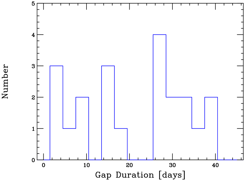
Figure 2: Histogram of the data gap duration, derived from the 21 data gaps found in the MAXI lightcurve (Figure 1).

As evident in Figure 1, Mrk 421 widely varied in the $3$ – $10$ keV range during the MAXI monitoring. In particular, several prominent X-ray flares were detected from the source. We have issued a quick alert for three of these flares (indicated by arrows in Figure 1), occurring on 2010 January 1, February 16, and 2011 September $7$ – $8$ (Isobe et al., 2010; Hiroi et al., 2011b). The lightcurve displays 21 data gaps, during which no X-ray flux was measured because the time bins failed the screening criteria described in §2.1. The duration of the data gap is distributed as shown in Figure 2. The average duration of the gaps is $21.1$ days.

3 PSD analysis

The PSD is commonly used to quantify the amplitude and timescale of intensity variation from various classes of astrophysical objects, including Galactic black hole binaries, Seyferts (e.g., Hayashida et al., 1998) and blazars (e.g., Kataoka et al., 2001). To estimate the PSD of Mrk 421, we adopted the periodogram normalized by the averaged source intensity after Miyamoto et al. (1991) and Hayashida et al. (1998);

$$P(f) = \frac{[a^{2}(f)+b^{2}(f)]T}{\mu^{2}},$$

$$a(f) = \frac{1}{n}\sum_{j=0}^{n-1}x_{j}\cos(2\pi ft_{j}),$$

$$b(f) = \frac{1}{n}\sum_{j=0}^{n-1}x_{j}\sin(2\pi ft_{j}),$$ (1)

where $f$ is the frequency of the intensity variation, $x_{j}$ is the source count rate at time $t_{j}$ ($0\leq j\leq n-1$), $n$ is the number of data points, $T$ ($=t_{n-1}-t_{0}$) is the total duration of the lightcurve, and $\mu$ is the unweighted average of the source count rate. Based on this definition, integration of the periodogram over the positive frequencies yields half of the excess variance. The underlying PSD, i.e., $S(f)$, of the source is evaluated by fitting a continuous function (such as a PL) to the observed periodogram. The Poisson level corresponding to the power due to the statistical fluctuation is calculated as

$$P_{\rm stat} = \frac{T\sigma_{\rm stat}^{2}}{n\mu^{2}}$$

$$\sigma_{\rm stat}^{2} = \sum_{j=0}^{n-1}\frac{(\Delta x_{\rm j})^{2}}{n}$$ (2)

where $\Delta x_{\rm j}$ denotes the error of the source count rate at $t_{j}$.

From the MAXI lightcurve of Mrk 421 in Figure 1, we can investigate the X-ray variability in the frequency range of $f=1\times 10^{-8}$ – $2\times 10^{-6}$ Hz, which has yet to be explored for blazars. However, to calculate the periodogram in equation (1), a continuous data stream with regular sampling (i.e., no data gaps) is required. To achieve this, we interpolated the missing time bin data by averaging the data in the five time bins (corresponding to 15 days) preceding and succeeding the missing bin (averaging over 10 bins in total). From these 10 time bins, those overlapping the gaps were discarded. The resulting continuous MAXI lightcurve of Mrk 421 is plotted as the dashed line in Figure 1. The interpolation procedure exerted only a minor effect on the weighted mean and standard deviation, which were re-evaluated as $2.0\times 10^{-2}$ counts cm^-2 s^-1  and $2.3\times 10^{-2}$ counts cm^-2 s^-1  respectively, in addition to the unweighted ones, $2.6\times 10^{-2}$ counts cm^-2 s^-1  and $2.7\times 10^{-2}$ counts cm^-2 s^-1 .

Before investigating the variability of Mrk 421, we analyzed the MAXI lightcurves of two bright galaxy clusters, the Coma Cluster and Centaurus Cluster, with X-ray fluxes of $2.5\times 10^{-10}$ ergs cm^-2 s^-1 and $9.3\times 10^{-11}$ ergs cm^-2 s^-1, respectively in the $4$ - $10$ keV range listed in the MAXI catalog (Hiroi et al., 2013). The flux of these sources is regarded as constant over the MAXI monitoring. We constructed the lightcurves and corresponding periodograms of both objects as described above. The periodogram of these sources became consistent with the Poisson level (i,e, $P(f)\sim P_{\rm stat}$), regardless of the variation frequency $f$. Therefore, we concluded that our interpolation technique exerted no significant systematic impact on the results of stable sources.

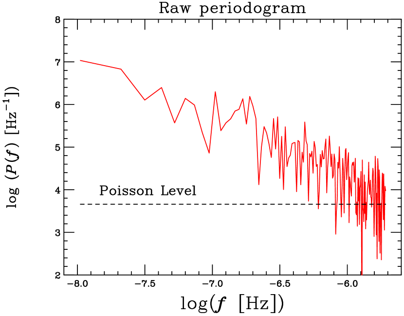
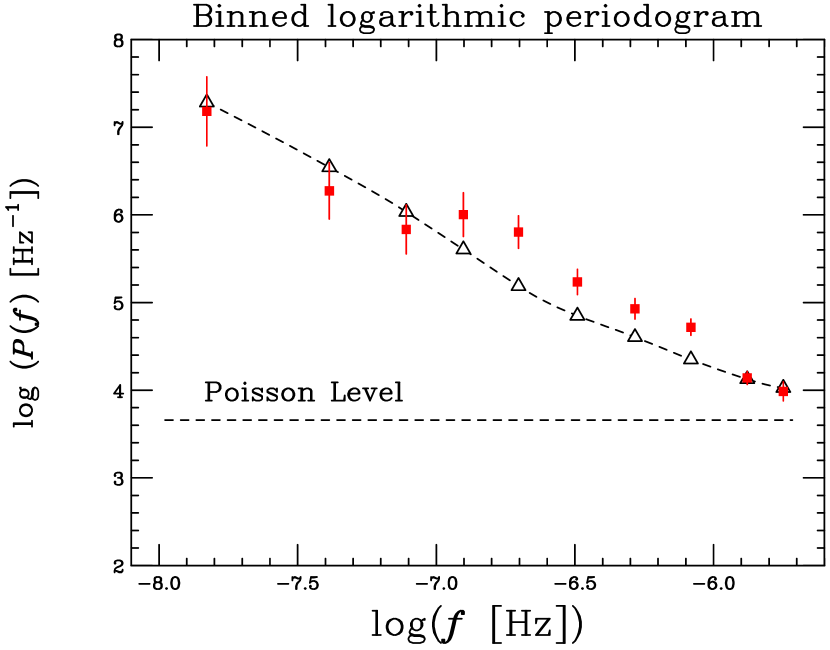
Figure 3: (Left) Raw periodogram derived from the MAXI GSC lightcurve of Mrk 421 in Figure 1. The level of the Poisson fluctuation ($P_{\rm stat}=4.56\times 10^{3}$ Hz^-1) is indicated by the horizontal dashed line. (Right) The binned logarithmic periodogram ($\overline{\log(P(f))}$), evaluated after Papadakis & Lawrence (1993), is plotted against the geometric mean frequency for each bin. The constant bias to the binned logarithmic periodogram was corrected by adding 0.25068 to $\overline{\log(P(f))}$ (Vaughan, 2005). The periodogram simulation for the best-fit PSD model ($\alpha_{\rm 0}=1.60$) is indicated by the open triangles, connected by the dashed line. Although the Poisson level was unsubtracted from the observed data, it is taken into account in the simulation.

The solid line in the left panel of Figure 3 presents the periodogram of Mrk 421 in the frequency range of $f=1\times 10^{-8}$ – $2\times 10^{-6}$ Hz evaluated by equation (1) from the interpolated MAXI lightcurve. Next, this raw periodogram was binned by a factor of 1.6 in the frequency. The frequency intervals were additionally bundled, such that each bin included at least two data points. Adopting the procedure proposed by Papadakis & Lawrence (1993), the average value of the logarithm of the raw periodogram, $\overline{\log(P(f))}$ (hereafter referred to as the binned logarithmic periodogram), was calculated for each bin, while its representative frequency was evaluated by the geometric mean frequency. Here, the Poisson level ($P_{\rm stat}=4.56\times 10^{3}$ Hz^-1) was not subtracted, because the several high-frequency data points are located below it, as shown in the left panel of Figure 3. The effect of the Poisson level is investigated through the simulation (see §5), when the best-fit PSD parameters are determined. Since the logarithm of the raw periodogram theoretically exhibits a constant variance of $\pi^{2}/6(\ln(10))^{2}=0.310$ (corresponding to the variance of $\log(\chi^{2}_{2}/2)$ where $\chi^{2}_{2}$ is the $\chi^{2}$ distribution with two degrees of freedom), the variance of the binned logarithmic periodogram was set at $\sigma_{\log(P(f))}^{2}=0.310/m$, with $m$ being the number of the data points in the individual bins. It is known that the binned logarithmic periodogram is biased as $\overline{\log(P(f))}=\log(S(f))-0.25068$ (e.g., Vaughan, 2005), where the constant offset of $-0.25068$ equals to the average of the $\log(\chi^{2}_{2}/2)$ distribution. Throughout the present paper, this offset is corrected by adding 0.25068 to $\overline{\log(P(f))}$. The right panel of Figure 3 displays the binned logarithmic periodogram. Over this frequency range, the periodogram appears to approximate a PL form.

4 PSD artifacts introduced by data gaps

The data gaps in the observed lightcurve can interfere with our PSD estimate. As shown in Figure 2, they persist over $3$ – $39$ days, corresponding to frequencies of $f=(0.3-4)\times 10^{-6}$ Hz. Above these frequencies the variability power may be over/underestimated by interpolating the data gaps. We thus investigated the influence of the gaps, using the simulation approach.

As described in Timmer & Koenig (1995, TK95), we produced 1000 simulated lightcurves in 3-day bins with PL-type underlying PSDs of the form $S(f)\propto f^{-\alpha_{0}}$. We, here, assumed an ideal case without any Poisson fluctuation (corresponding to $P_{\rm stat}=0$). A sampling pattern that exactly mimicked the observation was applied to the simulated data sets, yielding discontinuous artificial lightcurves. Following the processing procedure of the observed MAXI data, the fluxes in the gaps were interpolated and a periodogram, $P_{\rm s}(f)$, was derived from each simulated lightcurve. In the identical manner to that for the observed data, the binned logarithmic periodogram, $\overline{\log(P_{\rm s}(f))}$, was computed for each simulated periodogram. From the ensemble of the 1000 simulated products, the average and standard deviation of the binned logarithmic periodogram, $\langle\overline{\log{P_{\rm s}(f)}}\rangle$ and $\sigma_{\overline{\log{P_{\rm s}(f)}}}$ respectively, were evaluated for the individual frequency bins. By directly comparing $\overline{\log(P(f))}$ and $\langle\overline{\log{P_{\rm s}(f)}}\rangle$, we canceled out the effect of the data gaps. To correct for the effects of the red-noise leak (Papadakis & Lawrence, 1993), the transfer of power from lower to higher frequencies introduced by the limited observation period, lightcurves of 10-times-longer duration were initially created and divided into segments of 10 data sets. These processes were repeated for different values of the PL index $\alpha_{0}$.

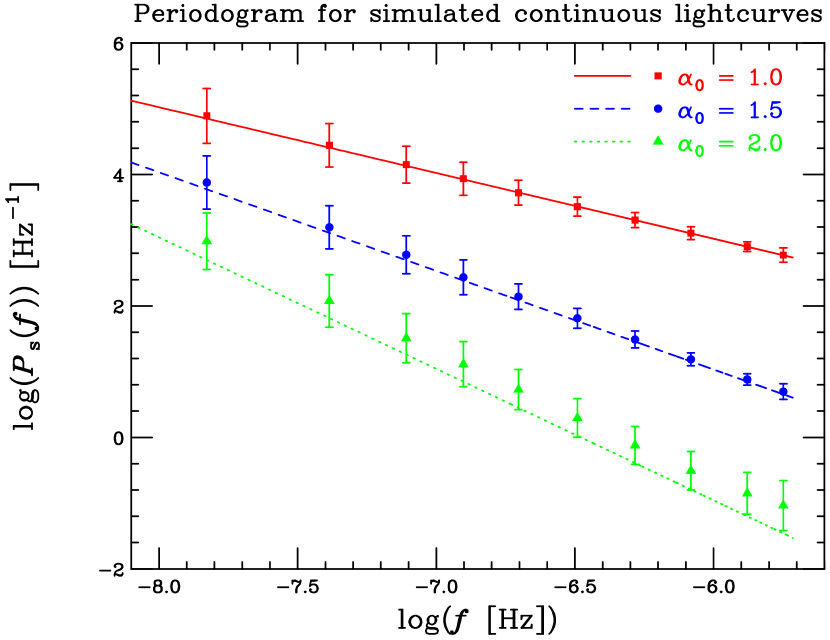
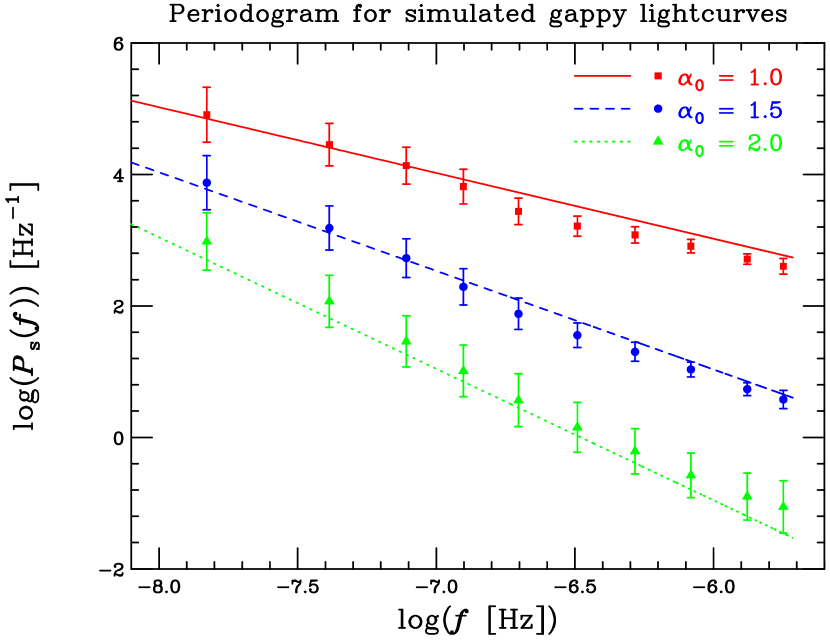
Figure 4: (Left) Binned logarithmic periodograms ($\langle\overline{\log{P_{\rm s}(f)}}\rangle$ and $\sigma_{\overline{\log{P_{\rm s}(f)}}}$) derived from the simulated continuous lightcurves without any data gaps, in comparison with the corresponding PSD model, $S(f)$. (Right) Binned logarithmic periodograms for the simulated discontinuous data sets, accounting for the data gaps. The results for the input PSD index $\alpha_{0}=1.0$, $1.5$ and $2.0$ are indicated by the red squares, blue circles, and green triangles, respectively, while the PSD models are plotted as the solid, dashed and dotted lines, respectively.

The left panel of Figure 4 compares $\langle\overline{\log{P_{\rm s}(f)}}\rangle$ derived from the simulated gapless data set with the PSD input to the simulations, $S(f)\propto f^{-\alpha_{0}}$, for the PSD index of $\alpha_{0}=1.0$, $1.5$ and $2.0$. The binned logarithmic periodogram from the simulation is found to coincide with the underlying PSD model for $\alpha_{0}=1.0$ and $1.5$, but overestimates the input PSD for $\alpha_{0}=2.0$, especially in the range of $f\gtrsim 5\times 10^{-7}$ Hz. The offset of $\langle\overline{\log{P_{\rm s}(f)}}\rangle$ from $\log(S(f))$ is attributable to red-noise leak, whose impact is predicted to be more significant at higher PSD indices (Papadakis & Lawrence, 1993).

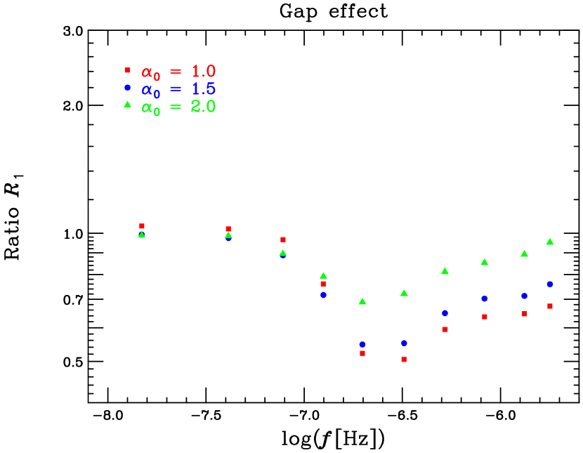
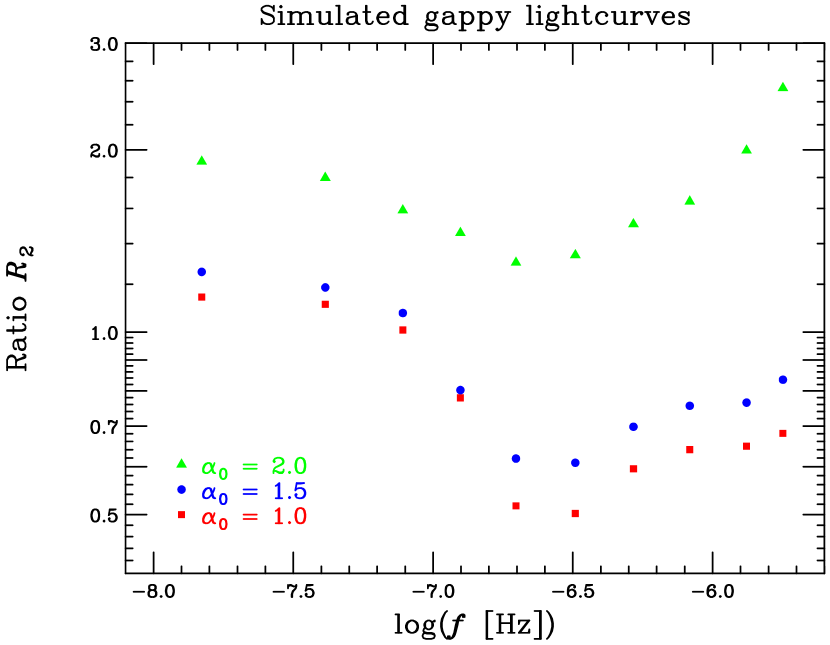
Figure 5: (Left) Ratio $R_{1}$ between the simulated periodograms considering and ignoring data gaps. Red squares, blue circles, and green triangles, show the results for input PSD indices $\alpha_{0}=1.0$, $1.5$, and $2.0$, respectively. (Right) Ratio $R_{2}$ of the periodogram from the simulated discontinuous lightcurves to the input PSD.

The right panel of Figure 4 plots $\langle\overline{\log{P_{\rm s}(f)}}\rangle$ derived from the simulations containing the data gaps. For the PSD indices $\alpha_{0}=1.0$ and $1.5$, for which the red-noise leak has a minor impact, the simulated periodogram clearly underestimates the input PSD $S(f)$, over the frequency range $f\sim 1\times 10^{-7}$ – $1\times 10^{-6}$ Hz. This frequency range corresponds to the timescale of the data gaps ($3$ – $39$ days; Figure 2). After the binned logarithmic periodogram was converted to the linear value as $10^{\langle\overline{\log{P_{\rm s}(f)}}\rangle}$, the ratio $R_{1}$ was evaluated between the simulated products with and without the data gaps. The left panel of Figure 5 indicates that the data gaps appear to artificially diminish the variability power around $f=(2$–$4)\times 10^{-7}$ Hz by a factor of up to $R_{1}\sim 1/2$. The right panel of Figure 5 displays the ratio $R_{2}$ of the periodogram derived from the simulated discontinuous lightcurves to the underlying PSD, defined as $R_{2}=10^{\langle\overline{\log{P_{\rm s}(f)}}\rangle}/S(f)$. In these results, the periodogram is less affected by the data gaps at frequencies $f\lesssim 1\times 10^{-7}$ Hz, where the ratio ranges are $0.7\lesssim R_{1}\lesssim 1.05$ and $0.8\lesssim R_{2}\lesssim 1.2$ for $\alpha\lesssim 1.5$.

5 Discussion

5.1 Comparison between the MAXI and ASCA data

Figure 6 plots the periodogram of Mrk 421  multiplied by the frequency (i.e., in the $fP(f)$ form) in the frequency range $f=1\times 10^{-8}$ – $2\times 10^{-6}$ Hz, derived from the 3 – 10 keV MAXI lightcurve. The MAXI periodogram is uncorrected for artifacts arising from data gaps and red-noise leak (investigated in §4). Here, we formally subtracted the Poisson level, after the binned logarithmic periodogram was translated into the linear value. For comparison, the periodogram of the source over the higher frequency range of $f=10^{-6}$ – $10^{-3}$ Hz, observed by ASCA in the $0.7$ – $7.5$ keV range, is also shown. Here, we adopt the ASCA data collected during the 1998 observation, of which the duration ($\sim 1$ week) is the longest among the three ASCA observations reported by Kataoka et al. (2001). The periodograms derived from the MAXI and ASCA data were not modified by any normalization scaling factors. It is important to note that a factor of 4 change was recorded in the variability power among the three ASCA observations.

Takahashi et al. (1996) reported that the shape of the SF of the Mrk 421 variability in the $0.07$ – $7.5$ keV range is energy independent from $10^{-2}$ to $3$ days. This suggests that the PSD shape of Mrk 421 is independent of the photon energy over the frequency range $f=10^{-6}$ – $10^{-3}$ Hz. Accordingly, we assumed that the PSD shape in the MAXI energy range ($3$ – $10$ keV) is similar to that in the ASCA range ($0.7$ – $7.5$ keV). At $2$ – $7.5$ keV, the observed variability power of the source is half that at $0.5$ – $2$ keV (Takahashi et al., 1996). Consequently, the PSD normalization is possible to differ between the MAXI and ASCA energy ranges by a factor of 2, at most.

Kataoka et al. (2001) reported that the periodogram of Mrk 421 above $f=10^{-5}$ Hz, derived from the 1998 ASCA observation, was reproduced by a PL-like PSD model with a slope of $\alpha_{\rm H}=2.14\pm 0.06$. They also revealed a PSD break at $f_{\rm b}=(9.5\pm 0.1)\times 10^{-6}$ Hz (as indicated by the blue dotted line in Figure 6). Although the error was large, the low frequency PSD index (below $f_{\rm b}$) was estimated as $\alpha_{\rm L}=0.88\pm 0.43$. In the remaining two ASCA data sets reported by Kataoka et al. (2001), the short observation duration ($\sim 1$ day corresponding to $f\gtrsim 10^{-5}$ Hz) precluded detection of a PSD break in these observations.

The MAXI data are critically important in constraining the PSD shape of the source at lower frequencies ($f<10^{-5}$ Hz). As shown in Figure 6, the periodogram derived from the MAXI data below $f=2\times 10^{-6}$ Hz appears flatter than that derived from ASCA above $f_{\rm b}$. In addition, both data sets indicate a similar variability power around $f\gtrsim 2\times 10^{-6}$ Hz. Thus, the MAXI data appear to qualitatively support the PSD break around the boundary between the MAXI and ASCA frequency ranges. However, to determine the underlying PSD shape in this frequency range, the artifacts of the data gaps must be deconvolved from the MAXI data (§5.2).

Similar to the analysis in §4, we simulated the MAXI periodogram for discontinuous lightcurves, by simply extending the best-fit PL PSD model to the ASCA data above the frequency break toward the lower frequency range of $f<2\times 10^{-6}$ Hz. The best-fit PSD index and normalization to the ASCA data was $\alpha_{\rm H}=2.14$ and $N_{\rm 0}=8.6\times 10^{2}$ Hz^-1 at $f_{\rm b}=9.5\times 10^{-6}$ Hz, respectively (Kataoka et al., 2001). The periodogram simulated by this model indicated by filled triangles in Figure 6 clearly exceed the observed data points over the entire MAXI frequency range. Even accounting for possible systematic PSD normalization factors between the MAXI and ASCA data sets, as discussed above, the simulated and actual MAXI data significantly differ. This implies that the PL-like PSD model fitted to the ASCA data above $f>10^{-5}$ Hz (i.e., $\alpha_{\rm H}=2.14$) does not smoothly extend into the MAXI frequency range. Thus, we roughly estimated a lower limit on the PSD break frequency as $f_{\rm b}\gtrsim 2\times 10^{-6}$ Hz, and successfully reinforced the ASCA result.

5.2 Low-frequency PSD Index

Next, we investigated the PSD shape of Mrk 421 in the frequency range $f=10^{-8}$ – $2\times 10^{-6}$ Hz by comparing the MAXI data with the simulated results in which the effects of the gap and red-noise leak were considered. The Poisson level was also included in the simulated periodograms, instead of subtracting it from the observed binned logarithmic periodogram. Over the MAXI range, the underlying PSD of the object was assumed to follow a simple PL function. The free parameters to be constrained in this model are the PSD normalization $N_{\rm 0}$ and the index $\alpha_{0}$. The normalization is evaluated at the putative break frequency $f_{\rm b}=9.5\times 10^{-6}$ Hz suggested from the ASCA data. Thus, the PSD function input to the simulation was $S(f)=N_{0}(f/f_{\rm b})^{-\alpha_{0}}$. Following the standard manner, the best-fit $N_{\rm 0}$ and $\alpha_{0}$ values were obtained by minimizing the $\chi^{2}$ function defined as

$$\chi^{2}=\sum_{j}\left(\frac{\overline{\log(P(f_{j}))}-\langle\overline{\log{P_{\rm s}(f_{j})}}\rangle}{\sigma_{\log(P(f_{j}))}}\right)^{2}$$ (3)

where $f_{j}$ denotes the frequency of $j$-th bin of the binned logarithmic periodogram with $j=0$ and $9$ corresponding to the lowest and highest frequency ones, respectively.

First, we attempted to constrain $\alpha_{0}$ and $N_{0}$, using all the 10 data points in the MAXI binned logarithmic periodogram, displayed in Figure 3. However, the fit was unsuccessful within the range $\alpha_{0}=0.5$ – $2.5$ and $N_{0}=10$ – $10^{5}$ Hz^-1 ($\chi^{2}/{\rm dof}\geq 23.5/8$), mainly because the MAXI data exhibit a hump feature over the $(2$ – $8)\times 10^{-7}$ Hz range. Using data collected by the All-Sky Monitor onboard the Rossi X-ray Timing Explorer, Osone et al. (2001) reported a possible peak in the PSD of Mrk 421 at $f=1.9\times 10^{-7}$ Hz, but did not rigorously evaluate its significance. Although the hump feature in the MAXI data resembles that of a quasi-periodic oscillation, its frequency exactly coincides with the frequency range of the artifacts introduced by the data gaps (Figure 5). We found that the hump cannot be readily disentangled from the gap artifacts using the MAXI data alone. Therefore, this feature is not further discussed in the present paper.

To reduce the effect of the data-gap artifacts and to avoid possible contamination from the hump structure, we next evaluated the PSD shape from the 6 data points with $j=0$ – $3$, $8$ and $9$, where the periodogram appears to be less affected by the gaps (i.e., where $R_{1}\gtrsim 0.7$ for $\alpha_{0}\sim 1.5$; left panel of Figure 5). Figure 7 displays the confidence contours on the $N_{\rm 0}$–$\alpha_{0}$ plane. The best-fit to the MAXI data was achieved at a PSD index and normalization $\alpha_{0}=1.60\pm 0.25$ and $N_{0}=4.4_{-3.0}^{+7.3}\times 10^{2}$ Hz^-1, respectively, ($\chi^{2}/{\rm dof}=4.0/4$), where the errors were evaluated at the 90% confidence level. The binned logarithmic periodogram simulated for the best-fit PSD model are overlaid on the right panel of Figure 3 with the open triangles. It is also plotted in Figure 6, after the Poisson level was subtracted in the similar manner to the observed data.

The variability power at the possible break determined from ASCA, $N_{\rm 0}=8.6\times 10^{2}$ Hz^-1 (Kataoka et al., 2001), is within the acceptable region of the MAXI data. Fixing the normalization at the ASCA value, the PSD index in the MAXI range is estimated as $\alpha_{0}=1.45_{-0.15}^{+0.10}$. Accounting for the possible uncertainty in $N_{0}$ discussed in §5.1 (a factor of 4 caused by PSD fluctuations in the ASCA observations and a factor of at most 2 introduced by the different energy coverage), the maximum systematic error in $\alpha_{0}$ is $\Delta\alpha_{0}\sim 0.4$. Therefore, we infer that the PSD slope in the MAXI frequency range is flatter than that above the break measured from the ASCA data ($\alpha_{\rm H}=2.14\pm 0.06$), but is consistent with the ASCA PSD slope below the break ($\alpha_{\rm L}=0.88\pm 0.43$), albeit with rather large errors. In the following discussion, we adopt the MAXI result for the low frequency PSD index of Mrk 421, since the MAXI data cover a wider frequency range below the break.

These results provide a quantitative support for the PSD break between the MAXI and ASCA frequency range. Surveying the $N_{\rm 0}$–$\alpha_{0}$ plane, we found that the PL model acceptable to the MAXI data intersects the extrapolation of the ASCA result above $f>1\times 10^{-5}$ Hz in the $f\geq 5\times 10^{-6}$ Hz range. This implies that the break suggested from the MAXI data is absolutely consistent with the ASCA result (Kataoka et al., 2001). Therefore, we concluded that the PSD of the X-ray variability of Mrk 421 breaks at $f_{\rm b}=(5$ – $9.5)\times 10^{-6}$ Hz. These results clearly demonstrate the utility of MAXI data for evaluating the longterm variability of blazars and, presumably, that of other classes of active galactic nuclei.

Investigating the X-ray lightcurves of the three archetypical VHE blazars (including Mrk 421), derived from ASCA long-look observations (exceeding $\sim 1$ week), Tanihata et al. (2001) identified a break in the SF at timescales of $\tau\sim 1$ day in all three blazars. In this case, the SF break at $\tau\sim 1$ day corresponds to a PSD break of $f_{\rm b}=1/\tau\sim 1\times 10^{-5}$ Hz, almost consistent with our result. However, Emmanoulopoulos et al. (2010), who conducted detailed lightcurve simulations, proposed that the SF break reported in Tanihata et al. (2001) was artificially induced by the ASCA observation period (i.e., $\gtrsim 1$ week). In contrast to the SF, the periodogram is reported to be relatively robust to artificial breaks introduced by truncated data lengths (Emmanoulopoulos et al., 2010). In §4, we also carefully simulated the artifacts from the data sampling window introduced to the MAXI periodogram. These analyses confirmed that the PSD of Mrk 421 breaks at $f_{\rm b}=(5$ – $9.5)\times 10^{-6}$ Hz (corresponding to the SF break at $\tau\sim$ a few days), where the results were derived by combining the MAXI and ASCA data sets.

Recently, Shimizu & Mushotzky (2013) investigated the hard X-ray lightcurve of Mrk 421 in the $14$ – $150$ keV energy range, extracted from 58-month observations by the Swift Burst Alert Telescope (BAT). They derived a hard X-ray PSD index of $\alpha=0.85\pm 0.25$ in the frequency range $f=10^{-8}$ – $10^{-6}$ Hz, significantly smaller than the MAXI result of $\alpha_{0}=1.60\pm 0.25$ in $3$ – $10$ keV. This result indicates that the X-ray variability pattern of Mrk 421 is energy-dependent especially toward the harder X-ray band, although no energy dependence was suggested in the PSD shape below $\sim 10$ keV (Takahashi et al., 2000). Otherwise, the PSD shape of Mrk 421 is possible to be variable in time, because the MAXI observation does not overlap with the 58-month BAT one.

5.3 Physical Implications

By making most of MAXI and ASCA, we confirmed that the PSD of the X-ray variability pattern from the VHE blazar Mrk 421 is significantly flatter in the lower frequencies ($f<2\times 10^{-6}$ Hz) than in the higher frequencies ($f>f_{\rm b}$). A steep PSD with an index of $\alpha_{\rm H}=2$ – $3$ in the $f\gtrsim 10^{-5}$ Hz range was commonly observed from the VHE blazars (Kataoka et al., 2001). This index is significantly higher than those of the the typical Seyfert galaxies, $\alpha=1$ – $2$, when their PSDs at $f=10^{-8}$ – $10^{-4}$ Hz were modeled by a single PL function (e.g., Uttley et al., 2002; Markowitz et al., 2003). The steep PSD of the VHE blazars has been widely ascribed to the physics operated in their jets, such as timescales related to the internal shocks (e.g., Kataoka et al., 2001).

Interestingly, the MAXI result on the PSD slope of Mrk 421 below the break frequency ($\alpha_{\rm 0}=1.60\pm 0.25$) agrees well with those of the typical Seyferts ($\alpha=1$ – $2$). Seyfert X-ray emission is believed to originate in the innermost region around the supermassive black hole and its accretion disk. The jet blobs observed in blazars may ultimately be ejected from the innermost disk, triggered by some disk instabilities. We thus speculate that the similarity of the PSD index over timescales longer than a few days (corresponding to $f<f_{\rm b}$) between blazars and Seyferts implies a physical connection between the activities in the jet and the innermost accretion disk (i.e., the activity of the accretion disk is possible to be propagated to the jets). However, PSD indices of $\alpha=1$ – $2$ are frequently observed in various classes of astrophysical objects, such as neutron star binaries (Fürst et al., 2010), magnetars (Huppenkothen et al., 2013), and so forth. Obviously, we cannot prove the disk-jet connection from the PSD shape alone. To confirm this scenario, we must construct a realistic model that simultaneously reproduce the PSDs of both blazars and Seyferts over a wide frequency range. Such an undertaking is beyond the scope of the present paper.

Table 1: X-ray sources detected within the Mrk 421 region

Source	(Ra, Dec )	$\Delta\theta$	$f_{\rm 4-10}$	$\sigma$
Mrk 421	($166.114$, $+38.209$)	—	$1.8\times 10^{-10}$	$107.1$
Src 1	($170.282$, $+42.214$)	$5^{\circ}.1$	$8.8\times 10^{-12}$	$6.0$
Src 2	($172.249$, $+36.339$)	$5^{\circ}.2$	$8.2\times 10^{-12}$	$6.2$

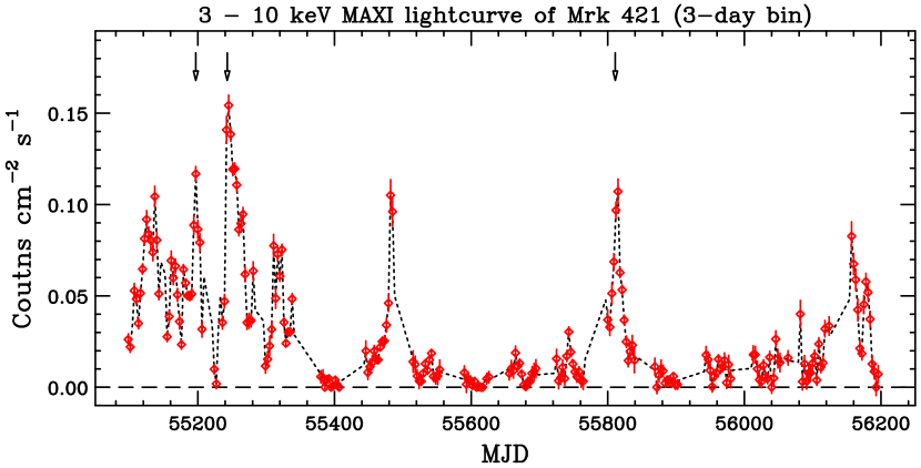
Figure 1: 3 – 10 keV MAXI GSC lightcurve of Mrk 421, covering 3 years between 2009 September 23 (MJD 55097) and 2012 October 15 (MJD 56215). Time resolution is 3 days. Red diamonds are data observed from the source. Unobservable periods (data gaps) have been filled by interpolating the real data (dotted line). The X-ray flares successfully alerted by MAXI (Isobe et al., 2010; Hiroi et al., 2011b) are indicated by arrows.

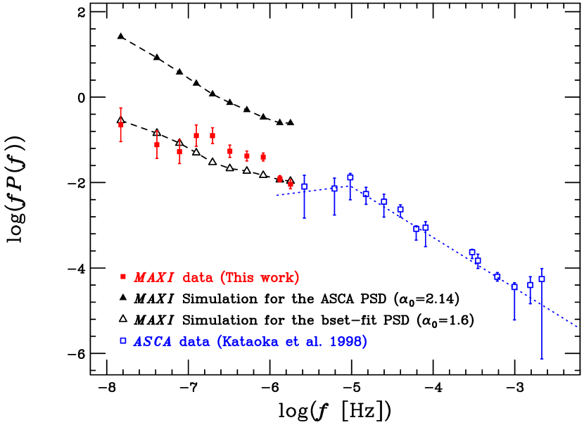
Figure 6: Comparison between the MAXI and ASCA periodograms, which are multiplied by frequency, shown in the logarithmic space (i.e., in the $\log(fP(f))$ form). The red filled squares indicate the MAXI data points (evaluated as $\log(f)+\overline{\log(P(f))}$), which were uncorrected for the artifacts introduced by the data gaps and red-noise leak (see §4). The Poisson level was subtracted. The blue open squares are taken from the long-look ASCA observation in 1998 (Kataoka et al., 2001). The ASCA data were reported to be successfully reproduced by a broken-PL PSD model (dotted line). The filled triangles show the simulated MAXI periodogram ($\log(f)+\langle\overline{\log{P_{\rm s}(f)}}\rangle$) when the PL PSD model with $\alpha_{0}=2.14$ that best-fitted the ASCA data above the break frequency ($f_{\rm b}=9.5\times 10^{-6}$ Hz) was simply extrapolated down to $f=1\times 10^{-9}$ Hz. The open triangles indicate the periodogram simulation of the best-fit PL model to the 6 MAXI data points ($\alpha_{0}=1.60$). All the simulation results account for the data gaps and red-noise leak.

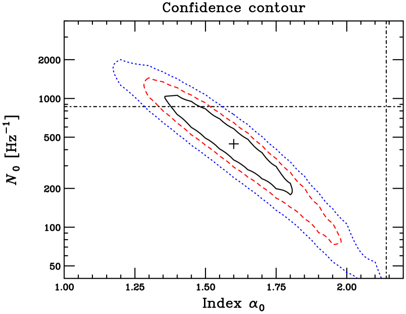
Figure 7: Confidence map on the plane of the PSD normalization $N_{\rm 0}$ and PSD index $\alpha_{\rm 0}$, derived from the 6 MAXI data points. The PSD normalization $N_{0}$ was evaluated at the possible break point suggested from the ASCA observation, $f_{\rm b}=9.5\times 10^{-6}$ Hz (Kataoka et al., 2001). The cross indicates the best-fit $N_{\rm 0}$ and $\alpha_{\rm 0}$ values ($\chi^{2}/{\rm dof}=4.0/4$). Three contours are drawn at the confidence levels of $68$%, $90$% and $99$% (i.e., corresponding to $\Delta\chi^{2}=2.30$, $4.61$ and $9.21$) with the black solid, red dashed and blue dotted lines, respectively. The horizontal and vertical dash-dotted lines indicate the best-fit values to the ASCA data above the break ($N_{0}=8.6\times 10^{2}$ Hz^-1 and $\alpha_{\rm H}=2.14$; Kataoka et al., 2001).

Appendix A Lightcurve simulation for an arbitrary PSD and PDF

The TK95 method, which we adopted for the lightcurve simulation, assumes that the count rate is strictly distributed in a Gaussian function. However, as shown in Figure 1, Mrk 421 exhibited a bursting behavior, indicating that the probability density function (PDF) of its lightcurve significantly deviates from Gaussianity. Recently, Emmanoulopoulos et al. (2013, E13) proposed a sophisticated technique to generate lightcurves satisfying simultaneously an arbitrary PSD and PDF. By comparing the results from these two methods, we briefly investigate systematic impacts on the PSD estimate due to the adopted simulation procedure.

At this point, we are only interested in approximately checking the sensitivity of our results to the lightcurve burstiness. Thus, we use some simplified forms of the input PSD and PDF, just for testing purposes.

Referring to §5.2, we simply adopted the PL-type underlying PSD model described as $S(f)=N_{0}(f/f_{\rm b})^{-\alpha_{0}}$. In order to generate lightcurves with the same statistics as for the observed one, the following condition was imposed (see Appendix of E13);

$$\frac{\sigma^{2}}{\mu^{2}}=2\int_{f_{1}}^{f_{2}}S(f)df,$$ (A1)

where $\mu=2.9\times 10^{-2}$ cts s^-1 and $\sigma=3.2\times 10^{-2}$ cts s^-1, respectively, is the unweighted average and standard deviation of the lightcurve (see §2.2), $f_{1}=1.05\times 10^{-8}$ Hz is the lowest frequency of the periodogram determined from the length of the lightcurve, and $f_{2}=1.93\times 10^{-6}$ Hz corresponds to the Nyquist frequency for the sampling time of $3$ days. Here, we assumed an idealized situation without any Poisson level.

We perform the lightcurve simulation for 3 cases, listed in Table 2. Case 2 represents the best-fit PSD model ($\alpha_{0}=1.60$; see Figure 7), derived from the 6 data points in the binned logarithmic periodogram, although its PSD normalization ($N_{0}=6.6\times 10^{2}$ Hz^-1) is different from the best-fit value ($N_{0}=4.4\times 10^{2}$ Hz^-1). There are two reasons for this discrepancy. The major one is that the hump feature in the observed MAXI periodogram was not considered in the best-fit PSD model as is visualized in Figure 6, while its power is taken into account in the PSD normalization employed here through equation (A1). The other minor reason is that we neglected the Poisson level, which also contributes to the observed standard deviation. The index of Cases 1 and 3 ($\alpha_{0}=1.40$ and $1.80$) is located near the edge of the acceptable range. Note that this section contains a rough implementation of the E13 method just for testing purposes.

Figure 8 plots the distribution of the count rate $x$, extracted from the observed MAXI lightcurve of Mrk 421. The figure confirms that the PDF is significantly far from the Gaussian function. We approximated the count rate histogram with a PDF model described as

$$p(x)=A_{1}\exp\left(-\frac{x}{B_{1}}\right)+A_{2}\exp\left(-\frac{x}{B_{2}}\right).$$ (A2)

The parameters in the function were tied as $A_{2}=\frac{1-A_{1}B_{1}}{B_{2}}$ so that the function meets the condition of $\int p(x)dx=1$ (i.e., the definition of the PDF). As is shown with the solid line in Figure 8, the model was found to reasonably reproduce the observed histogram ($\chi^{2}/{\rm dof}=1.66$) with the parameters tabulated in Table 3. We employed this solution as the input PDF model to the lightcurve simulation by the E13 procedure. We have to be careful about the fact that this PDF model is affected by the data gaps (while the gap effect was subtracted from the input PSD model as shown in §5.2). It is important to note that the standard deviation corresponding to the PDF model ($\sigma=4.2\times 10^{-2}$ cts s^-1) is higher than that of the observed lightcurve, when we integrate it over the range of $x=0$ – $\infty$. This is due to the long tail of the PDF function toward higher count rates, even though its integrated probability at $x>0.16$ is less than 2%. If we limit the count rate at $x\leq 0.16$ cts s^-1, where the observed data points are distributed, the standard deviation becomes consistent to the observed value.

For each parameter set (i.e., Cases 1 – 3), we generated 1000 lightcurves by the E13 technique. We confirmed that the average count rate and standard deviation input to equation (A1) were reproduced in the simulated products for all the cases. After the the data gaps in the observed lightcurve are applied, the individual simulated lightcurves were converted to the binned logarithmic periodogram with the procedure explained in §4. The ensemble average and standard deviation were evaluated from the 1000 binned logarithmic periodograms, in the similar manner to the TK95 simulation.

The binned logarithmic periodograms from the E13 and TK95 simulations are found to coincide with each other within their scatters (i.e., the standard deviations). After the averaged values of the binned logarithmic periodogram from these two methods were re-converted to linear values, we found that the E13 result is smaller by only a factor of $1$ – $2$ than the TK95 result for all the cases. Therefore, we have concluded that our result is relatively insensitive to the adopted simulation technique.

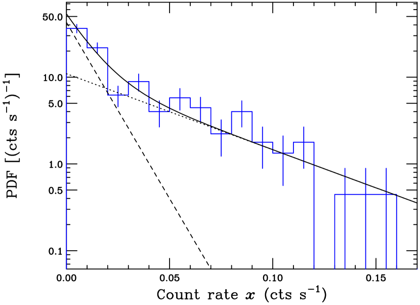
Figure 8: PDF of the observed MAXI lightcurve plotted as a function of the count rate $x$. The solid line indicates the best-fit model function $p(x)$, defined in equation (A2). The two exponential components of $p(x)$ are shown the dotted and dashed lines.

Table 2: Parameters of the underlying PSD model.

Case	$\alpha_{0}$	$N_{0}$ (Hz-1)
1	$1.40$	$1.9\times 10^{3}$
2	$1.60$	$6.6\times 10^{2}$
3	$1.80$	$2.2\times 10^{2}$

Table 3: Best-fit PDF parameters

Parameter	$A_{1}$ (cts s$-^{-1}$)-1	$B_{1}$ cts s-1	$A_{2}$ (cts s$-^{-1}$)-1	$B_{2}$ cts s$-^{-1}$
Value	$42.78$	$0.0107$	$10.95$	$0.0495$

References

- Abramowski et al. (2013) Abramowski, A. et al., 2013, A&A, 550, A4
- Albert et al. (2008) Albert, J., et al., 2008, ApJ, 681, 944
- Błażejowski et al. (2000) Błażejowski, M., Sikora, M., Moderski, R., & Madejski, G.M., 2000, ApJ, 545, 107
- Cash (1979) Cash, W., 1979, ApJ, 228, 939
- Cohen et al. (1976) Cohen, M.H., et al., 1976, ApJ, ApJ, 206 L1
- Dermer & Schlickeiser (1993) Dermer, C.D. & Schlickeiser, R. 1993, ApJ, 416, 458
- Eguchi et al. (2009) Eguchi, S., Hiroi, K., Ueda, Y. Sugizaki, M., Tomida, H., Suzuki, M., & the MAXI Team, 2009, Proceedings of Astrophysics with All-Sky X-Ray Observations – 3rd international MAXI Workshop (JAXA-SP-08-014E), 44
- Emmanoulopoulos et al. (2010) Emmanoulopoulos, D., McHardy, I.M. & Uttley, P., 2010, MNRAS, 404, 931,
- Emmanoulopoulos et al. (2013) Emmanoulopoulos, D., McHardy, I.M. & Papadakis, I.E., 2013, MNRAS, 433, 907 (E13)
- Fosatti et al. (1998) Fossati, G., Maraschi, L., Celotti, A., Comastri, A., & Ghisellini, G. 1998, MNRAS, 299, 433
- Fürst et al. (2010) Fürst, F., 2010, A&A, 519, 37
- Ghisellini et al. (1998) Ghisellini, G., Celotti, A., Fossati, G., Maraschi, L., & Comastri, A., 1998, MNRAS, 301, 451
- Górski et al. (2005) Górski, K.M., Hivon, E., Banday, A.J., Wandelt, B.D., Hansen, F.K., Reinecke, M., & Bartelmann, M., 2005, ApJ, 622, 759
- Hayashida et al. (1998) Hayashida, K., Miyamoto, S., Kitamoto, S., Negoro, H., & Inoue, H., 1998, ApJ, 500, 642
- Hiroi et al. (2011a) Hiroi, K., et al., 2011a, PASJ, 63, S677
- Hiroi et al. (2011b) Hiroi, K., et al., 2011b, The Astronomer’s Telegram, #3637
- Hiroi et al. (2013) Hiroi, K., et al. 2013, ApJS, 207, 36
- Huppenkothen et al. (2013) Huppenkothen, D., et al., 2013, ApJ, 768, 87
- Isobe et al. (2010) Isobe, N., et al., 2010, PASJ, 62, L55
- Jorstad et al. (2005) Jorstad, S.G., et al. 2005, AJ, 130, 1418
- Kataoka et al. (2001) Kataoka, J., et al., 2001, ApJ, 560, 659
- Kino et al. (2002) Kino, M., Takahara, F., & Kusunose, M., 2002, ApJ, 564, 97
- Kirsch et al. (2005) Kirsch, M.G, et al., 2005, SPIE, 5898, 22
- Markowitz et al. (2003) Markowitz, A., et al., 2003, ApJ, 593, 96
- Matsuoka et al. (2009) Matsuoka, M., et al., 2009, PASJ, 61, 999
- Mihara et al. (2011) Mihara, T., et al., 2011, PASJ, 63, 623
- Mitsuda et al. (2007) Mitsuda, K., et al. 2007, PASJ 59, S1-S7
- Miyamoto et al. (1991) Miyamoto, S., Kimura, K., Kitamoto, S., Dotani, T., & Ebisawa, K., 1991, ApJ, 383, 784
- Nolan et al. (2012) Nolan, P.L., et al., 2012, ApJS, 199, 31
- Osone et al. (2001) Osone, S., & Teshima, M., 2001, Proceedings of the 27th International Cosmic Ray Conference (Hamburg), 2695
- Papadakis & Lawrence (1993) Papadakis, I.E., & Lawrence, A., 1993, MNRAS, 261, 612
- Pearson et al. (1981) Pearson, T.J., Unwin, S.C., Cohen, M.H., Linfield, R.P., Readhead, A.C.S., Seielstad, G.A., Simon, R.S., & Walker, R. C., 1981, Nature, 290, 365
- Shimizu & Mushotzky (2013) Shimizu, T.T., & Mushotzky, R.F., 2013, ApJ, 770, 60
- Sikora et al. (1994) Sikora, M., Begelman, M. C., & Rees, M. J., 1994, ApJ, 421, 153
- Simonetti et al. (1985) Simonetti, J.H., Cordes, J.M., & Heeschen, D.S., 1985, ApJ, 296, 46
- Sugizaki et al. (2011) Sugizaki, M., et al., PASJ, 63, 635
- Takahashi et al. (1996) Takahashi, T., et al., 1996, ApJ, 470, 89
- Takahashi et al. (2000) Takahashi, T., et al., 2000, ApJ, 542, L105
- Tanaka et al. (1994) Tanaka, Y., Inoue, H., & Holt, S.S., 1994, PASJ, 46, 37
- Tanihata et al. (2001) Tanihata, C., Urry, C. M., Takahashi, T., Kataoka, J. Wagner, S.J.; Madejski, G.M., Tashiro, M., & Kouda, M. 2001, ApJ, 563, 569
- Tanihata et al. (2003) Tanihata, C., Takahashi, T., Kataoka, J., & Madejski, G.M., 2003, ApJ, 584, 153
- Timmer & Koenig (1995) Timmer, J., & König, M., 1995, A&A, 300, 707 (TK95)
- Uttley et al. (2002) Uttley, P., McHardy, I.M., & Papadakis, I.E., 2002, MNRAS, 332, 231
- Vaughan (2005) Vaughan, S., 2005, A&A, 431, 391