Consistency of dark matter interpretations of the 3.5 keV X-ray line

Abstract

Tentative evidence of a 3.5 keV X-ray line has been found in the stacked spectra of galaxy clusters, individual clusters, the Andromeda galaxy and the galactic center, leading to speculation that it could be due to decays of metastable dark matter such as sterile neutrinos. However searches for the line in other systems such as dwarf satellites of the Milky Way have given negative or ambiguous results. We reanalyze both the positive and negative searches from the point of view that the line is due to inelastic scattering of dark matter to an excited state that subsequently decays—the mechanism of excited dark matter (XDM). Unlike the metastable dark matter scenario, XDM gives a stronger signal in systems with higher velocity dispersions, such as galaxy clusters. We show that the predictions of XDM can be consistent with null searches from dwarf satellites, while the signal from the closest individual galaxies can be detectable having a flux consistent with that from clusters. We discuss the impact of our new fits to the data for two specific realizations of XDM.

I Introduction

A surprising new hint of dark matter emerged from analysis of data from XMM-Newton, in which the spectra of 73 galaxy clusters were combined, showing $>3\sigma$ evidence for an X-ray line with energy 3.55 keV Bulbul:2014sua . It was argued that there were no plausible atomic transitions to account for such a line, but that it could come from the decay of light dark matter (DM) such as sterile neutrinos. Further evidence for the line was found in the spectra of the Perseus cluster and (less prominently) of the Andromeda galaxy Boyarsky:2014jta . A subsequent search for the line in the center of the Milky Way using Chandra data gave negative results Riemer-Sorensen:2014yda whereas a similar search using XMM-Newton data corroborated the line Boyarsky:2014ska . Ref. Anderson:2014tza stacked spectra of 81 and 89 galaxies using Chandra and XMM-Newton data, respectively, finding no evidence for the line, while ref. Malyshev:2014xqa searched for the line in stacked spectra of nearby dwarf spheroidal galaxies, also with negative results. The latter two papers emphasize that there is a definite contradiction to the decaying dark matter interpretation made by ref.  Bulbul:2014sua , at the level of $3.3-4.6$ $\sigma$ for ref. Malyshev:2014xqa and $4.4-11.8$ $\sigma$ for ref. Anderson:2014tza . Previous searches for X-ray lines are reviewed in ref. Boyarsky:2012rt . Most recently (after the first version of this work), ref. Urban:2014yda reported a positive flux using Suzaku data from the Perseus cluster but only upper limits from other nearby clusters.

There is also controversy as to whether an atomic origin for the line is really excluded. Ref. Jeltema:2014qfa argues that transitions of ionized potassium and chlorine explain the line reported by Bulbul:2014sua ; Boyarsky:2014jta . Counterarguments have been given in Boyarsky:2014paa ; Bulbul:2014ala . We do not enter into this debate in the present paper (however see ref. Iakubovskyi:2014yxa for a recent synopsis). Instead we will assume that the line is due to new physics, namely dark matter scattering rather than decays. The kinematical differences between the two processes can explain why an X-ray line would be seen in some data sets and not in others. In particular, if the scattering is inelastic with a small energy threshold, one expects the strongest signal to come from from galaxy clusters, while that from dwarf galaxies would be highly suppressed, and line strengths from nondwarf galaxies would be somewhere between these two extremes.

As a concrete realization of this alternative phenomenology, we focus on a class of dark matter models in which inelastic scattering of two DM particles to excited states, $\chi\chi\to\chi^{\prime}\chi^{\prime}$, is followed by rapid decays $\chi^{\prime}\to\chi\gamma$ Finkbeiner:2007kk ; Pospelov:2007xh ; Finkbeiner:2014sja ; Frandsen:2014lfa . We refer to this as the excited dark matter (XDM) mechanism. The DM need not be as light as 7.1 keV, as in the metastable decaying models; it can be heavy, requiring only the mass splitting between $\chi^{\prime}$ and $\chi$ to be 3.55 keV. Specific examples of XDM models for addressing the 3.55 keV X-ray signal were considered in refs. Cline:2014eaa ; Cline:2014kaa .

The papers that searched for the line signal derived limits (or observed ranges) for the mixing angle $\theta_{\nu}$ of a Majorana sterile neutrino, decaying through its transition magnetic moment to an active neutrino. The mixing angle is related to the partial width for the decay by Boyarsky:2005us

$$\Gamma_{\nu} = {9\,\alpha\,G_{F}^{2}\over 1024\,\pi^{4}}\,\sin^{2}2\theta_{\nu}\,m_{\nu}^{5}$$ (1)

$$= 2.46\times 10^{-28}{\rm s}^{-1}\,{\sin^{2}2\theta\over 10^{-10}}\,\left(m_{\nu}\over 7.1\,{\rm keV}\right)^{5}$$

Ref. Bulbul:2014sua finds the best fit for $\sin^{2}2\theta\cong 6\pm 3\times 10^{-11}$. Ref. Boyarsky:2014jta obtains a consistent result, with larger errors. Ref. Anderson:2014tza finds the $3\sigma$ upper limit $\sin^{2}2\theta\ <2\times 10^{-11}$, while Malyshev:2014xqa obtains $\sin^{2}2\theta\ <(2.7-4.8)\times 10^{-11}$, depending upon different assumptions about the contribution from decays of DM in the main halo of the Milky Way. Ref. Riemer-Sorensen:2014yda finds somewhat weaker limits $\sin^{2}2\theta\ <(5-10)\times 10^{-11}$, depending upon the energy interval that is modeled. These results are summarized in table 1.

(1)	(2)	$\ (3)\ \nu$ mixing	(4) fast decay	(5) intermediate	(6) slow decay	(7) $v$ disp.
Reference	object	$\quad\sin^{2}2\theta_{\nu}$	${\langle\sigma v\rangle_{f}\cdot\left(10\,{\rm GeV}\over m_{\chi}\right)^{2}}^{\phantom{|}}$	$\tau\sim 2\times 10^{6}$y	${\langle\sigma v\rangle_{s}\cdot\left(10\,{\rm GeV}\over m_{\chi}\right)^{2}}^{\phantom{|}}$	$\quad\langle\sigma_{v}\rangle$
		$\ (\times 10^{-11})$	($10^{-22}\,{\rm cm}^{3}{\rm s}^{-1}$)	or $2\times 10^{7}$y	($10^{-22}\,{\rm cm}^{3}{\rm s}^{-1}$)	(km/s)
Bulbul et al. Bulbul:2014sua	clusters	$\quad\ \ 6\pm 3$	$\quad 480\pm 250$		$\quad\ 1200\pm 600$	$\ \ \ 975$
Bulbul et al. Bulbul:2014sua	Perseus	$\quad(26-60)$	$\quad(1400-3400)$		$\ \ (4000-15000)$	$\ \ 1280$
Boyarsky et al. Boyarsky:2014jta	Perseus	$\quad(55-100)$	$\ \ (1-2)\times 10^{5}$		$\ \ \ (1-5)\times 10^{4}$	$\ \ 1280$
Urban et al. Urban:2014yda	Perseus	$\quad(20-100)$	$\ \ (2600-4100)$		$\ \ \ (1-2)\times 10^{4}$	$\ \ 1280$
Bulbul et al. Bulbul:2014sua	CCO	$\quad(18-28)$	$\quad(1200-2000)$		$\quad(5100-8400)$	$\ \ \ 926$
Boyarsky et al. Boyarsky:2014jta	M31	$\quad(2-20)$	$\quad\ \left\{\begin{array}[]{ll}(10-30),&{\rm NFW}\\ (30-50),&{\rm Burkert}\end{array}\right.$	${{\rm NFW}\atop\to}\left\{{{\rm unchanged}\atop(20-50)}\right\}$	$\ \quad(370-970)$	$\ \ \ 116$
Boyarsky et al. Boyarsky:2014ska	MW	$\quad(10-30)$	$\quad\left\{\begin{array}[]{ll}(0.1-0.7),&{\rm NFW}\\ (50-550),&{\rm Burkert}\end{array}\right.$	${{\rm NFW}\atop\to}\left\{{(1-8)\atop(16-110)}\right\}$	$\quad\ (400-3000)$	$\ \ \ 118$
Riemer-Sørensen Riemer-Sorensen:2014yda	MW	$<(6-20)$	$\ <\left\{\begin{array}[]{ll}(0.15-1.1),&{\rm NFW}\\ (80-1200),&{\rm Burkert}\end{array}\right.$	${{\rm NFW}\atop\to}\left\{{(2-12)\atop(24-170)}\right\}$	$\ <(200-2000)$	$\ \ \ 118$
Anderson et al. Anderson:2014tza	galaxies	$<(2-5)$	$\ <(270-620)$		$\ <(170-420)$	$\ \ \ 100$
Malyshev et al. Malyshev:2014xqa	dwarfs	$<(3-5)$	$\ <(0.2-0.3)$		$\ <(0.1-0.2)$	$\ \ \ \ 10$
Bulbul et al. Bulbul:2014sua	Virgo	$<(18-23)$	$<(380-670)$		$\ <(2.5-4.1)\times 10^{4}$	$\ \ \ 643$
Urban et al. Urban:2014yda	Coma	$<(1.5-1.7)$	$\ \ <(130-200)$		$\ <(510-850)$	$\ \ \ 913$

Table 1: Column 3: best-fit values or upper limits on the sterile neutrino mixing angle, $\sin^{2}2\theta$, assuming $\nu_{s}\to\nu\gamma$ for the 3.55 keV X-ray line. Column 4: corresponding values of the cross section for excited dark matter models with $\chi\chi\to\chi^{\prime}\chi^{\prime}\to\chi\chi\gamma\gamma$ for the case of prompt decay of $\chi^{\prime}$. For fast decays of XDM in the Milky Way, fits are given both to NFW and Burkert profiles. Column 5: for the case of excited state lifetimes $\tau\sim 2\times 10^{6}\,$y or $2\times 10^{7}\,$y the MW cross sections change relative to NFW values in column 4 as shown, while others are unaffected. Column 6: same as column 4 but for slow decays (lifetime of order the dynamical time scale). Column 7: average velocity dispersion. Values for Coma, Centaurus clusters from ref. Girardi:1995iy , and for Ophiuchus from 2010MNRAS.405.1624M .

In this work, we will systematically derive the corresponding values for the phase-space-averaged cross section $\langle\sigma v\rangle$ that plays the role of $\Gamma_{\nu}$ for the XDM scenario. We do using the predicted X-ray fluxes from the two models:

$$F_{\gamma} = \quad\,\Gamma_{\nu}\left<\int{d^{\,3}x\over 4\pi\,x^{2}}\,{\rho\over m_{\nu}}\right>,\quad{\rm decays}$$ (2)

$$= \langle\sigma v\rangle_{f}\left<\int{d^{\,3}x\over 4\pi\,x^{2}}\,{\rho^{2}\over m_{\chi}^{2}}\right>,\quad{\rm XDM}$$ (3)

Here $\rho$ is the DM mass density, the origin of $\vec{x}$ is at the observer, and $m_{\nu}=7.1$ keV for decaying DM, while $m_{\chi}$ can be much larger in the XDM model. The subscript on $\langle\sigma v\rangle_{f}$ refers to the assumption that $\chi^{\prime}$ decays relatively fast, as we will discuss further below. The large angle brackets indicate that an average over different sources is typically being carried out, be they dwarf galaxies, normal galaxies, or clusters of galaxies. By performing this average in the same way for XDM as it was carried out by the original authors we can convert their determinations of $\Gamma_{\nu}$ into corresponding values for $\langle\sigma v\rangle$. However in most cases we can work directly from the reported fluxes using eq. (3). This is the first objective of our work. We will then show how the expected DM velocity dependence of $\langle\sigma v\rangle$ can make the derived values consistent with an XDM origin for the observed line.

We identify a small discrepancy in the inferred cross sections (and neutrino mixing angles) for the Milky Way and Andromeda galaxy (M31), despite similar velocity dispersions, if we assume a standard NFW profile. However, if the Milky Way’s DM halo is slightly cored rather than cuspy, the amount of DM in the field of view is reduced, leading to a larger value of the required cross section. Since a similar change does not affect the line-of-sight integral (3) much for M31 due to the greater distance, we find that slight coring removes the discrepancy.

So far we implicitly assumed that the excited state decays immediately, but it is also possible that it could be sufficiently long-lived that it migrates significantly before decaying. In the extreme case where the lifetime is of the same order as the dynamical time scale for the object of interest, the excited states become distributed evenly throughout the halo, and the brightness profile of the X-ray line has the same shape as for decaying DM, although the overall predicted rate differs from that of purely decaying DM. In that case the photon flux takes the same form as in (2), but with the replacements $m_{\nu}\to m_{\chi}$ and $\Gamma_{\nu}\to\Gamma_{\rm eff}$, where the effective decay rate given by

$$\Gamma_{\rm eff}=\left<{\langle\sigma v\rangle_{s}\,\int{d^{\,3}x}\,\rho^{2}\over m_{\chi}\,\int{d^{\,3}x}\,\rho}\right>={\langle\sigma v\rangle_{s}\over m_{\chi}}\left<\rho_{s}{h_{2}(c)\over h_{1}(c)}\right>$$ (4)

with the integrals extending out to the virial radius $R_{\rm vir}$ of the halo. $\rho_{s},\ r_{s}$ are the respective scale density and length for the DM distribution, to be defined below, and $h_{1,2}(c)$ are dimensionless functions of the concentration parameter $c=R_{\rm vir}/r_{s}$, given in the appendix. The subscript on $\langle\sigma v\rangle_{s}$ denotes that $\chi^{\prime}$ is assumed to decay slowly. In the following we will carry out our analysis for both extremes of the excited state lifetime, as well as intermediate cases. We will show that lifetimes of order $10^{6}-10^{7}\,$y provide an alternate resolution to the discrepancy between the galactic center and M31 fluxes.

In the remaining sections II-VIII we determine the required values or upper limits for the cross sections from galaxy clusters, M31, the Milky Way, the Perseus cluster, dwarf spheroidals, and stacked galaxies respectively. In section IX we show how these can be fit to general parameters of the XDM class of models. The implications for two specific models are considered in section X, followed by our conclusions.

II Galaxy clusters

Ref. Bulbul:2014sua combines spectra of 73 galaxy clusters. For each cluster the integral $\int d^{\,3}x\,\rho/x^{2}$ (called $M^{proj}_{DM}/D^{2}$ in Bulbul:2014sua ) is determined within a given field of view (FOV), defined by an extraction radius $R_{ext,i}=\theta_{i}d_{i}$ where $\theta_{i}$ is the angular size of the observed region and $d_{i}=D$ is the distance to the source. The relative exposure ${Exp}_{i}$ for each source is also given.

For each cluster, an NFW profile is assumed,

$$\rho_{\rm\scriptscriptstyle NFW}={\rho_{s,i}\over(r/r_{s,i})(1+r/r_{s,i})^{2}}$$ (5)

The scale radius is taken to be $r_{s,i}=R_{500,i}/c_{500}$ where $R_{500,i}$ is the radius of a sphere whose average density is $500$ times the critical density of the universe, and the concentration parameter is a weakly-varying function of the virial mass that is in the range $c_{500}\sim 3-4$ for most clustersvik . For the more distant clusters, $R_{500,i}=R_{ext,i}$, which is tabulated in ref. Bulbul:2014sua . But for the closer ones, $R_{500}$ exceeds the XMM-Newton $700^{\prime\prime}$ field of view (FOV). In order to determine the NFW parameters for all clusters in a consistent way, we assume (as did Bulbul:2014sua ) a universal value of the concentration parameter, which implies that all clusters have the same value of $\rho_{s}=\delta_{c}\rho_{\rm crit}$, where the critical density is given by $\rho_{\rm crit}=1.25\times 10^{11}M_{\odot}/$Mpc³ (ignoring small redshift-dependent corrections) and $\delta_{c}=(500/3)c^{3}/h_{1}(c)$ (see for example ref. Urban:2014yda ). We then determine $r_{s}$ for each cluster by equating the projected mass tabulated in Bulbul:2014sua to $M^{proj}_{DM}=4\pi\rho_{s}r_{s}^{3}f_{1}(R_{\rm ext}/r_{s})$, where $f_{1}$ is given in eqs. (21).

Once the parameters of $\rho_{\rm\scriptscriptstyle NFW}$ are known, it is straightforward to compute $\int d^{\,3}x\,\rho^{2}/x^{2}$ for each cluster and average them, weighting by the exposures ${Exp}_{i}$. Taking $\Gamma_{\nu}=1.74\times 10^{-28}\,$s^-1 corresponding to ref. Bulbul:2014sua ’s best-fit mixing angle, we obtain from eqs. (2-3) the cross section $\langle\sigma v\rangle_{f}=5.5\times 10^{-20}\,$cm${}^{3}\,$s${}^{-1}\times(m_{\chi}/10{\rm\ GeV})^{2}$, in the case of promptly decaying excited states, assuming $c=3$, and $4.1\times 10^{-20}\,$cm${}^{3}\,$s${}^{-1}\times(m_{\chi}/10{\rm\ GeV})^{2}$ for $c=4$. This gives some idea as to the uncertainties $(\sim 15\%)$ due to the DM halo properties. In table 1 we combine this in quadrature with the significantly larger $(50\%)$ uncertainty from the measured flux.

For slowly decaying $\chi^{\prime}$, we equate $\Gamma_{\nu}/m_{\nu}=\Gamma_{\rm eff}/m_{\chi}$ from (4) and (2) to find

$$\langle\sigma v\rangle_{s}=\Gamma_{\nu}{m_{\chi}^{2}\,h_{1}\over m_{\nu}\,h_{2}}\rho_{s}^{-1}$$ (6)

leading to the higher values $(0.95-1.4)\times 10^{-20}\,$cm${}^{3}\,$s^-1 for $c=3-4$.

III Andromeda Galaxy

Ref. Boyarsky:2014jta attributes a flux of $F_{\gamma}=4.9{+1.6\atop-1.3}\times 10^{-6}$/cm²/s to a combined FOV of radius 0.22${}^{\circ}(\equiv\!\theta)$ centered on M31. We follow Boyarsky:2014jta in adopting the best-fit NFW profile of ref. Corbelli:2009nc for M31, with $r_{s}=23.8\,$kpc and $\rho_{s}=4.3\times 10^{6}\,M_{\odot}$/kpc³.  Taking the distance to be $d=778\,$kpc, hence $a=\theta d/r_{s}=0.13$, we compute the integral of $\rho^{2}/x^{2}$ and find the cross section $\langle\sigma v\rangle=m_{\chi}^{2}F_{\gamma}d^{2}/(\rho_{s}^{2}r_{s}^{3}f_{2}(a))=2.1\times 10^{-21}\,$cm${}^{3}\,$s${}^{-1}\times(m_{\chi}/10{\rm\ GeV})^{2}$ for fast decays. Alternatively, ref. klyp finds best-fit values of $r_{s}=25\,$kpc (also with $c=12$, and $R_{\rm vir}=300\,$kpc, $M_{\rm vir}=1.6\times 10^{12}M_{\odot}$) and $\rho_{s}=5.0\times 10^{6}\,M_{\odot}$/kpc³, giving $1.4\times 10^{-21}\,$cm${}^{3}\,$s^-1. The uncertainty due to the density profile is somewhat smaller than that from the line flux for the overall uncertainty in the cross section. In table 1 we give the range of values that includes both uncertainties.

For slowly-decaying DM, we find, using

$$\langle\sigma v\rangle_{s}={F_{\gamma}\,m_{\chi}^{2}\,d^{2}\,h_{1}(c)\over\rho_{s}^{2}\,r_{s}^{3}}=\langle\sigma v\rangle_{f}{f_{2}(a)\,h_{1}(c)\over f_{1}(a)\,h_{2}(c)}$$ (7)

from (4) and (20), that the cross sections increase to $970\times 10^{-22}$ and $370\times 10^{-22}\,$cm${}^{3}\,$s^-1 respectively, for the two halo profiles. In table 1 we give the ranges including the uncertainty in the flux $F_{\gamma}$.

We have also explored the effect of a cored versus cuspy DM halo. Ref. Tempel:2007eu fits the M31 DM halo to several profiles including NFW (cuspy) and Burkert (cored), the latter being given by

$$\rho_{\rm B}(r)={\rho_{s}\over(1+r/r_{s})(1+r^{2}/r_{s}^{2})}$$ (8)

with best fit values $r_{s}=6.86\,$kpc, $\rho_{s}=5.72\times 10^{7}\,M_{\odot}/$kpc³ for Burkert. The LOS integral of $\rho^{2}$ over the 0.22^∘ FOV differs only by a factor of 1.1-1.7 relative to the NFW profiles considered above, and so we conclude that the cusp versus core issue is not a great source of uncertainty for M31. We will see however that it is much more important for the Milky Way.

IV The Milky Way

Ref. Riemer-Sorensen:2014yda obtains upper limits on the flux of X-ray lines in the energy intervals 3-6 and 2-9 keV, based upon Chandra observations of a $16^{\prime}\times 16^{\prime}$ region at the galactic center, with the central disk of angular size $2.5^{\prime}$ excised. For simplicity we model this region by an annulus of equivalent area with $2.5^{\prime}<\theta<9^{\prime}$. The limits on the flux at photon energy 3.55 keV are found to be 12.1 and $21.4\times 10^{-6}$ counts/cm²/s respectively for the two energy intervals (see footnote 1).

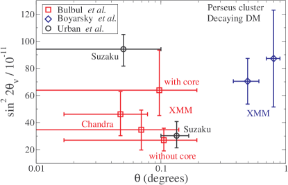
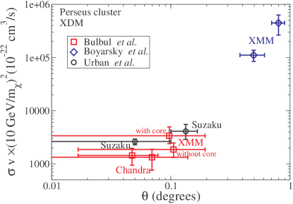
Figure 1: Left: mixing angle of decaying sterile neutrino that would give the measured fluxes for Perseus in the angular intervals indicated by horizontal error bars. Vertical bars correspond to errors in fluxes. Right: similar to left, but showing the cross section for excited dark matter models. Perseus data alone would favor the decaying DM scenario, or possibly XDM with slow decays of the excited state.

We apply these flux limits directly to find the corresponding limits on $\Gamma_{\nu}$ and $\langle\sigma v\rangle$ using eqs. (2,3). To explore the dependence upon the assumed Milky Way DM profile, we first compute $\int d^{\,3}x\,\rho^{n}/x^{2}$ for a range of NFW profiles suggested by simulations (see ref. read ), with $r_{s}=19{+7.5\atop-5.4}\,$ kpc at 68% confidence, and varying the local density $\rho_{\odot}$ between $(0.3-0.4)$ GeV/cm³ while keeping the distance $r_{\odot}$ to the GC fixed at $8.3\,$kpc. (The effect of a cored profile will be considered below.) Varying $r_{s}$, $\rho_{s}$ and the limit on the flux leads to the range of upper limits the neutrino mixing angle $\sin^{2}2\theta<(6-20)\times 10^{-11}$ and on the cross section $\langle\sigma v\rangle(10{\rm\,GeV}/m_{\chi})^{2}<(0.15-1.1)$ in units of $10^{-22}$cm³/s, for the case of fast decays. Repeating this for the $1\sigma$ range of Milky Way NFW profiles found in ref. Nesti:2013uwa , we get the smaller range of $\langle\sigma v\rangle(10{\rm\,GeV}/m_{\chi})^{2}<(0.07-0.15)$. The larger range is shown in table 1.

On the other hand, ref. Boyarsky:2014ska finds positive evidence for the line from the inner $14^{\prime}$ of the GC using XMM-Newton data, with a flux of $(29\pm 5)\times 10^{-6}$ counts/cm²/s which is consistent with the previous bounds at the $2\sigma$ level. Following the same procedure as for the upper limits, we find the allowed ranges of the cross section to be $(0.11-0.65)\times 10^{-22}$cm³/s for the DM profiles reported in ref. read .

For slowly decaying excited states, again using (7) we find that the range of upper limits from Riemer-Sorensen:2014yda becomes $(0.19-1.7)\times 10^{-19}$cm³/s, while the range of measured values from Boyarsky:2014ska is $(0.39-2.7)\times 10^{-19}$cm³/s. These are much larger than the corresponding M31 values because of the large factor $f_{2}|^{a_{2}}_{a_{1}}/f_{1}|^{a_{2}}_{a_{1}}=320$ for the MW in eq. (7), compared to $\sim 1$ for M31.

Because the FOV is so strongly concentrated on the galactic center for the MW observations, the model predictions are extremely sensitive to the assumed behavior of the DM profile in this region. Ref. Nesti:2013uwa prefers the Burkert profile (8) as the best fit to the MW. The LOS integral of $\rho^{2}$ is much smaller with the best fit cored profiles shown in fig. 3 of Nesti:2013uwa than the corresponding NFW profiles also fit there, by a factor of 500-1000. In table 1 we give the ranges of cross sections for fast decays in these cored profiles as well as in the NFW profiles. These are extreme cases, and one could expect the true profile to give cross section values somewhere in between. Because of this uncertainty, the MW observations might be considered not very constraining when trying to distinguish between different kinds of DM models.

V Perseus Cluster

Ref. Bulbul:2014sua obtains several flux measurements of the line, centered on the Perseus cluster using XMM and Chandra data. In two of them, the central region of radius $1^{\prime}$ is removed because of large X-ray fluxes possibly having an origin from atomic transitions in the core of the cluster. These have fluxes of $21.4{+7.0\atop-6.3}$ with XMM MOS and $10.2{+3.7\atop-3.5}$ with Chandra ACIS-S, in units of $10^{-6}$cm^-2s^-1, and respective fields of view $700^{\prime\prime}$ and $281^{\prime\prime}$ (approximating the square by a circle of equivalent area) in radius, minus the excised central region. There are also two measurements including the core, with fluxes of $52.0{+24.1\atop-15.2}$ from XMM MOS and $18.6{+7.8\atop-8.0}$ from Chandra ACIS-I. More recently ref. Urban:2014yda measured nonzero fluxes using Suzaku data, with $F_{\gamma}=2.87{+0.33\atop-0.38}\times 10^{-7}$cm^-2s^-1arcmin${}^{-2}\times 36\pi\,$arcmin² from the central $0.1^{\circ}$, and $F_{\gamma}=4.78{+1.65\atop-1.41}\times 10^{-8}$cm^-2s${}^{-1}\times(18^{2}-36\pi)$ from a surrounding region going out to $0.17^{\circ}$. We model the fields of view as annular regions of equivalent area.

To evaluate the LOS integrals, we use the DM density profile determined by ref. Simionescu:2011ii . It finds virial mass and radius $M_{200}=6.65{+0.43\atop-0.46}\times 10^{14}M_{\odot}$ and $R_{200}=1.79\pm 0.04\,$Mpc, and concentration parameter $c_{200}=5.0\pm 0.5$, leading to NFW scale radius $r_{s}=R_{200}/c=0.36\pm 0.04\,$Mpc, and density $\rho_{s}=M_{200}\,c^{3}/(4\pi\,R_{200}^{3}\,h_{1}(c))=(1.2\pm 0.3)\times 10^{15}M_{\odot}/$Mpc³, where the values are anticorrelated with those of $r_{s}$ via the dependence upon $c$ and we ignore the smaller error due to $M_{200}$. We take the distance to the cluster to be $d=74\,$Mpc.

The data divided by the LOS integrals in (2) or (3) are plotted in fig. 1, so that consistency with a given model should result in no dependence on the angle from the center. The data at low angles do not show a clear preference for decaying versus annihilating or scattering DM models, but including those at larger off-center angles would disfavor scattering (XDM) relative to decays. Ref. Boyarsky:2014jta reports X-ray fluxes of $(13.8\pm 3.3)$ and $(8.3\pm 3.4)\times 10^{-6}$/cm²/s in two off-center angular bins with $\theta=(0.38^{\circ}-0.61^{\circ})$ and $(0.7^{\circ}-0.9^{\circ})$ respectively, and with average field of view 537 arcmin². We model the fields of view by part of an annular region bounded by the polar angles $\theta_{i}$ given above, and an azimuthal interval $\delta\phi$ such that $\delta\phi(\cos\theta_{2}-\cos\theta_{1})=537$ arcmin². Then $\delta\phi=75.1^{\circ},\,53.4^{\circ}$ respectively for the two bins, and we can take $\delta\phi/360^{\circ}$ times the formula (20) for the density integrals when applying (3) or (7). (For annular regions bounded by two polar angles, one must replace $f_{2}(a)/f_{1}(a)\to f_{2}|^{a_{2}}_{a_{1}}/f_{1}|^{a_{2}}_{a_{1}}$.)

Although the Perseus data by themselves appear to be more consistent with decaying DM than with XDM, one should keep in mind that the mixing angle required by the combined Perseus observations is in tension with limits from the Coma cluster, dwarf spheroidals and stacked galaxies to be discussed below, suggesting that the DM signal, if present, may be contaminated by other backgrounds.  Ref. Urban:2014yda notes that the evidence for the line in Perseus disappears if a sufficiently complex model of atomic line backgrounds is adopted. Moreover, the large signal at large off-center angles might be consistent with the hypothesis that baryons in clusters tend to be concentrated at the outskirts due to transport by shock waves Rasheed:2010pq . On the other hand, the XDM model can reconcile some of the Perseus data with the upper limits. In our XDM fits to the data, we will treat the large-angle observations and those including the core as outliers and retain only the lower-angle noncore fluxes reported by Bulbul:2014sua . Including the data of ref. Urban:2014yda deteriorates the quality of the fits somewhat but does not change the shape of the allowed regions significantly.

VI Other nearby clusters

Ref. Bulbul:2014sua finds a positive signal from combining spectra of nearby clusters Coma, Centaurus and Ophiuchus (CCO), with averaged flux $F_{\gamma}=15.9{+3.4\atop-3.8}\times 10^{-6}/$cm${}^{2}/$s over the XMM MOS $700^{\prime\prime}$ field of view. The respective weighting factors for averaging the spectra are $0.35,\,0.51,\,0.14$ bulbul . In addition, a 90% confidence level upper limit of $F_{\gamma}<9.1\times 10^{-6}/$cm${}^{2}/$s on the flux from the Virgo cluster was found using Chandra ACIS-I with $500^{\prime\prime}$ FOV. More recently, ref. Urban:2014yda obtained 95% c.l. upper limits on the line fluxes from Suzaku spectra of Coma, Virgo and Ophiuchus, with that from Coma giving the most stringent constraints on dark matter models: $F_{\gamma}<2.65\times 10^{-9}/$cm${}^{2}/s$/arcmin${}^{2}\times(18{\rm\ arcmin})^{2}$.

To translate these into DM model constraints we follow the procedure of ref. Urban:2014yda for determining the NFW halo parameters, similar to the one which we employed for the stacked clusters: a universal concentration $c_{200}=4.1$ is assumed, implying $\rho_{s}=\delta_{c}\rho_{\rm crit}=7\times 10^{14}M_{\odot}/$Mpc³, while the scale radius is given in terms of virial masses as $r_{s}^{3}=M_{200}/(4\pi\rho_{s}h_{1}(c))$. As in Urban:2014yda we take $M_{200}=(8.54,\,1.40,\,1.47)\times 10^{14}M_{\odot}$ respectively for Coma, Virgo and Ophiuchus, while for Centaurus we take $M_{200}=3\times 10^{14}M_{\odot}$, which follows from the average temperature $kT=3.68$ keV Horner:1999wf and the $M_{200}$-$T$ scaling relation of Arnaud:2005ur .

Using these parameters and eqs. (2-3), we find from the CCO observation the values for the mixing angle and cross section given in table 1 (with uncertainties due to the halo profile estimated by varying $c=3-4$), roughly compatible with the values obtained by the same authors for the Perseus cluster. The upper limits from Virgo are also marginally compatible with these values. However the limit on the mixing angle from the Coma cluster flux limit of ref. Urban:2014yda is quite stringent, $\sin^{2}2\theta_{\nu}\lesssim 2\times 10^{-11}$, and at odds with the values indicated by the other positive observations of the line. The limit on the XDM cross section from Coma on the other hand is in a lesser degree of tension, $\langle\sigma v\rangle_{f}<200\times 10^{-22}$cm³/s for $m_{\chi}=10$ GeV, only marginally below the range of values indicated by the stacked clusters.

VII Dwarf spheroidal limits

Malyshev et al. Malyshev:2014xqa give limits on the neutrino mixing angle from XMM-Newton observations of eight dwarf spheroidal galaxies in the Milky Way. In their analysis, no assumption was made as to the shape of the dwarf density profiles, since they approximate $\int d^{\,3}x\,\rho/x^{2}=M_{FOV}/d^{2}$, where $M_{FOV}$ is the DM mass within the FOV and $d$ is the distance to the dwarf spheroidal. This enclosed mass was estimated in a way that was assumed to be relatively independent of the particular profile.

However for DM scattering, the signal goes like $\rho^{2}$ and can thus have a stronger dependence on the profile shape. Here we consider the possibilities that the dwarf density profiles are either NFW as in eq. (5) or cored, with $\rho_{\rm cored}=\rho_{s}/(1+r/r_{s})^{3}$. Following ref. Walker:2009zp that presents evidence for universal density profiles for dwarf spheroidal galaxies, we take $r_{s}=0.795\,$kpc for each NFW profile, and $r_{s}=0.150\,$kpc for cored, deriving the corresponding XDM limits on $\langle\sigma v\rangle$ for both cases.

Moreover ref. Malyshev:2014xqa accounts for the flux from the Milky Way halo, for which the profile is taken to be NFW, but with two possible values of the scale radius and normalization, klyp . These are $r_{s}=21.5\,$kpc, $\rho_{s}=4.9\times 10^{6}M_{\odot}/$kpc³ and $r_{s}=46\,$kpc, $\rho_{s}=0.6\times 10^{6}M_{\odot}/$kpc³, respectively, and referred to as the “mean” and “minimal” halo models. The total DM density is thus $\rho=\rho_{s}+\rho_{MW}$ in each observed dwarf field of view (FOV), complicating the evaluation of the integral of $\rho^{2}/x^{2}$, which we carry out numerically. (Analytic expressions for the contributions from the dwarf halo densities $\rho_{s}$ alone are given in the appendix, and were used to check the numerics.) The angular radius of the FOV is taken to be the minimum of $\theta_{1/2}=r_{1/2}/d_{i}$ and the XMM-Newton FOV, $15^{\prime}$.

Ref. Malyshev:2014xqa tabulates the distance to each dwarf, its half-light radius $r_{1/2}$ (where the intensity profile of its visible light output drops by a factor of 2 relative to the center), and the mass $M_{1/2}$ enclosed within $r_{1/2}$. These are sufficient for determining the parameters $\rho_{s}$ for either the NFW or the cored profile each dwarf, given the assumed values of $r_{s}$ mentioned above. The only further information required for computing $\int d^{\,3}x\,\rho^{2}/x^{2}$ is the angle $\phi_{i}$ between the line of sight (LOS) to the dwarf and that to the galactic center, since the DM density of the Milky Way halo along the LOS to the dwarf depends upon $\phi_{i}$. This angle is related to the galactic coordinates $(b,l)$ of the dwarf by $\cos\phi=\cos(b)\cos(l)$. We find that $\cos\phi_{i}=\{-0.159,\,0.052,\,-0.224,\,-0.455,\,-0.183,\,-0.704,\,-0.510,$ $-0.496\}$ respectively for the satellites Carina, Draco, Fornax, Leo I, Ursa Minor, Ursa Major II, Willman I, and NGC 185. The distance to the GC is taken to be 8.5 kpc for consistency with Malyshev:2014xqa .

The expected fluxes for the decaying neutrino model are given in Malyshev:2014xqa , so we need not recompute $\int d^{\,3}x\,\rho/x^{2}$ in (2). It can be deduced from the fluxes using the limit on the decay rate $\Gamma_{\nu}<6.68\times 10^{-29}\,$s^-1 that we infer from the limit on the mixing angle $\sin^{2}2\theta<2.67\times 10^{-11}$ for the mean MW model. These limits are weaker by a factor of 1.78 for the minimal MW model. Carrying out the $\rho^{2}$ integrals and weighting them by the exposures given in Malyshev:2014xqa , we find the following limits on $\langle\sigma v\rangle(10{\rm\,GeV}/m_{\chi})^{2}$, in units of $10^{-22}$cm³/s: for the NFW dwarf profiles, 0.18 and 0.26 respectively, in the mean and minimal MW halo models; for the cored dwarf profiles, we obtain the same values to two significant figures, thus finding little difference between cored versus NFW profiles, although there is some dependence upon the assumed shape of the MW halo.

VIII Limit from stacked galaxy spectra

Ref. Anderson:2014tza finds a limit of $\sin^{2}2\theta<0.47\times 10^{-10}$ for a decaying neutrino with $m_{\nu}=7.1$ keV, from stacking Chandra spectra of 81 galaxies. The authors obtain a somewhat stronger limit of $\sin^{2}2\theta<0.19\times 10^{-10}$ from XMM-Newton data for 89 galaxies. They assume NFW profiles for which the scale radii are related to the virial radius as $r_{s}=R_{\rm vir}/c_{200}$, where the concentration parameter is related to the virial mass $M_{\rm vir}$ as determined by ref. Prada:2011jf . The relation can be fit by $\log_{10}c_{200}=1.85-0.08\log_{10}M_{\rm vir}$ (where $M_{\rm vir}=M_{200}$ is in units of $h^{-1}M_{\odot}$) for $\log_{10}M_{\rm vir}<14.6$, and remaining constant for higher masses. Ref. Anderson:2014tza tabulates $R_{\rm vir}$ and $M_{\rm vir}$ (also called $M_{\rm halo}$ in that reference) as well as the distances to each galaxy. This allows us to construct the NFW profiles for their galaxies (using $\rho_{s}=M_{\rm vir}/(4\pi r_{s}^{3}h_{1}(c))$) to calculate the quantities in eq. (2-3).

To avoid sensitivity to the central cusp of the NFW distribution (which may not be present in realistic simulations accounting for effects of baryons), the signal is taken between $r=0.01$ and $1$ times $R_{\rm vir}$ of each galaxy. Analytic expressions can be found for the LOS integrals for NFW density (and density-squared) profiles (see appendix). We compute the exposure-time-weighted averages of the density integrals separately for the Chandra and XMM-Newton data to obtain the equivalent limits on $\langle\sigma v\rangle(10{\rm\,GeV}/m_{\chi})^{2}$ for the two data sets. The limit on $\langle\sigma v\rangle_{f}$ is related to that on the decay rate by $\Gamma_{\nu}(m_{\chi}^{2}/m_{\nu})\langle M_{\rm vir}f_{1}|^{c}_{0.01c}d^{-2}h_{1}^{-1}(c)\rangle/$ $\langle M_{\rm vir}\rho_{s}f_{2}|^{c}_{0.01c}d^{-2}h_{1}^{-1}(c)\rangle$ for fast decays, and for slow decays the relation is $\langle\sigma v\rangle_{s}=$ $\Gamma_{\nu}(m_{\chi}^{2}/m_{\nu})\langle(h_{2}/h_{1})\rho_{s}\rangle^{-1}$. From table 1 we see that the resulting limits on XDM are less constraining than the claimed observations from M31 or MW, and so we can omit this constraint from the fits we undertake next.

IX Compatibility of XDM with data

Decaying dark matter is ostensibly at odds with the required values of the lifetime (here parametrized by the sterile neutrino mixing angle) for the claimed observations, versus the upper limits from null searches. Superficially, it would appear that the same is true for annihilating DM models or XDM, from the required values versus upper limits for the annihilation or excitation cross section. However for XDM there is an additional parameter, since the cross section depends upon the DM velocity due to the energy threshold needed to create the excited states. In the center-of-mass frame, this corresponds to the relative velocity threshold

$${v_{t}/c}=\sqrt{8\,\delta m_{\chi}/m_{\chi}}$$ (9)

The kinetic energy of the scattering DM particle is $m_{\chi}(v_{t}/2)^{2}/2=\delta m_{\chi}$, necessary for creating the excited state with mass $m_{\chi}+\delta m_{\chi}$. This can be used to explain why the X-ray signal from XDM would be stronger in systems with larger DM velocities.

Indeed, the phase space averaged cross section depends upon the velocity dispersion of the DM, $\sigma_{v}=\langle v^{2}\rangle^{1/2}=\sqrt{3/2}\,v_{0}$ (where $v_{0}$ is the circular velocity), corresponding to an assumed Maxwellian distribution $f(v)=Ne^{-(v/v_{0})^{2}}$. The averaged cross section can be approximated as

$$\langle\sigma v\rangle = \sigma_{0}v_{t}\gamma,$$ (10)

$$\gamma = \left\langle\sqrt{v_{\rm rel}^{2}/v_{t}^{2}-1}\,\,\Theta(v_{\rm rel}-v_{t})\right\rangle,$$ (11)

and $\langle F(v_{\rm rel})\rangle=\int d^{3}v_{1}d^{3}v_{2}f(v_{1})f(v_{2})F(|\vec{v}_{1}-\vec{v}_{2}|)$, assuming that there is no significant velocity-dependence in the cross section other than that coming from the phase space integral. The functional form of $\gamma(v_{0}/v_{t})$ is plotted in ref. Cline:2014kaa (and will appear in our figures showing fits to the data below). For $v_{0}>v_{t}$, it is approximately linear, while for $v_{0}<v_{t}$ it falls exponentially,

$$\gamma\cong 1.4\left\{\begin{array}[]{ll}(v_{0}/v_{t}),&v_{0}\gtrsim 1.3\,v_{t}\\ e^{-(v_{t}/v_{0})^{2}/2},&v_{0}\lesssim 0.3\,v_{t}\end{array}\right.$$ (12)

For $v_{0}\sim v_{t}$ there is intermediate behavior that smoothly connects these two expressions.

This additional dependence can explain why no X-ray signal is seen from dwarf ellipsoidal galaxies, whereas it is strong enough in galaxy clusters and nondwarf galaxies. However, it cannot explain the fact that the Perseus cluster seems to give a much stronger line relative to other galaxy clusters, especially at large off-center angles. To pursue the DM explanation, we must assume that these large-angle Perseus observations are contaminated by some background, as was suggested by ref. Bulbul:2014sua , or else that only the Perseus observations are indicative of DM decays, and that the other positive claims are somehow spurious. On the other hand, the error bars on the on-center Perseus measurements are sufficiently large that they do not greatly diminish the goodness of our fits if we include them. In the following, we will show results of fits in which Perseus fluxes are treated as outliers that require further explanation, but we will also indicate the effect of the on-center Perseus fluxes in the computation of the $\chi^{2}$, using the Bulbul et al. values shown in table 1 for the required value of the cross section.

To estimate the average velocity dispersion $\sigma_{v}$ for clusters, we have identified $\sigma_{v}$ for 22 out of the 73 clusters studied by Bulbul et al. using ref. struble ; see table 2. Their average $\sigma_{v}$ is 1055 km/s, and their average weighted by the exposures of ref. Bulbul:2014sua is 975 km/s.

name	$\sigma_{v}$	name	$\sigma_{v}$	name	$\sigma_{v}$	name	$\sigma_{v}$
Perseus	1282	A262	588	A478	904	A496	714
A665	1201	A754	931	A963	1350	A1060	647
A1689	1989	A2063	659	A2147	821	A2218	1370
A2319	1770	A2811	695	A3112	950	A3558	977
A2390	1686	A3571	988	A3581	577	A3888	1831
A4038	882	A4059	628

Table 2: Clusters from ref. Bulbul:2014sua whose velocity dispersions $\sigma_{v}$ (in km/s) are tabulated in ref. struble .

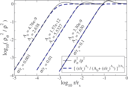
Figure 2: Solid curves: ratio of smeared $\rho^{2}$ to original $\rho^{2}$, eq. (13), for NFW profile with smearing lengths $\sigma=(0.1,\,0.01,\,0.001)\,r_{s}$ (from right to left), and approximate analytic fits (dashed curves).

IX.1 M31 versus Milky Way

We have seen that for NFW DM profiles, there is a discrepancy between the X-ray line strengths from M31 and from the Milky Way, which require seemingly incompatible values of the cross section. Basically the claimed signal from the very small field of view of the MW (relative to its virial radius) should be much higher for a NFW profile, to be compatible with that from M31. This suggests that the density of decaying excited states is lower in this central region than predicted. We have identified two ways of addressing this: (1) the lifetime of the excited state is long enough for the particles to stream out of the central region before decaying; (2) the halo profile is less cuspy than NFW. We will consider both of these possibilities in the following.

IX.1.1 Intermediate lifetime of excited state

Table 1 indicates a dramatic increase in the required scattering cross sections for the case of slow decays versus fast ones suggesting that there exist some intermediate values of the lifetime where the XDM interpretation of M31 and MW fluxes could be made compatible. It is important to realize that the MW observation has a FOV that covers only the inner part of the halo with $r/r_{s}<10^{-3}$, whereas the M31 observation covers a much larger fraction $r/r_{s}<0.13$. This implies that a relatively short excited state lifetime $\tau$ (compared to the dynamical timescale for galaxies) could be enough to deplete the inner region of the MW due to DM transport during time $\tau$, reducing the signal there and boosting the required value of $\langle\sigma v\rangle$, whereas it would have a small effect on the observed region of M31.

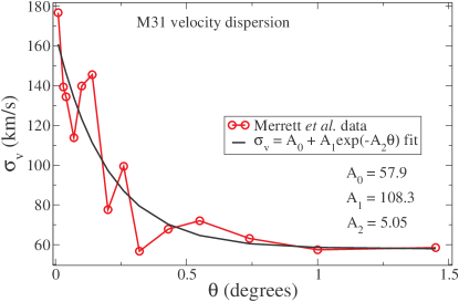
Figure 3: Measurements of M31 velocity dispersion from ref. merrett , and an analytic fit to the data.

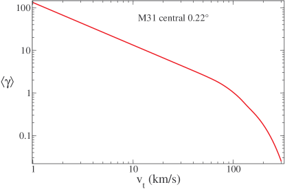
Figure 4: Average value of $\gamma$, eq. (11), $\langle\gamma\rangle=[\int d^{\,3}x\,\gamma\rho^{2}/x^{2}]/[\int d^{\,3}x\,\rho^{2}/x^{2}]$, integrated over the $1.5^{\circ}$ FOV of the M31 observations in ref. Boyarsky:2014jta .

To model the effect of a relatively short excited state lifetime, we will assume that the flux formula (3) holds, but with $\rho^{2}$ replaced by a smeared version,

$$\rho^{2}(x)\to\rho^{2}_{\sigma}=N\int d^{\,3}x^{\prime}\,e^{-(\vec{x}-\vec{x}^{\prime})^{2}/\sigma^{2}}\,\rho^{2}(x^{\prime})$$ (13)

where $\sigma$ is the streaming length of the excited states before they decay, $\sigma\sim\sigma_{v}\tau$, with $\sigma_{v}$ being the velocity dispersion. We consider the relevant values $\sigma=(10^{-3},\,10^{-2},\,10^{-1})\,r_{s}$ (taking for simplicity $r_{s}=23.8\,$kpc for both M31 and MW). By numerically evaluating the integral in (13) for an NFW density profile, we find that $\rho^{2}_{\sigma}$ is given by a function that can be approximated as

$${\rho_{\sigma}^{2}\over\rho^{2}}\cong\left((r/r_{s})^{A_{1}}\over A_{0}+(r/r_{s})^{A_{1}}\right)^{2/A_{1}}$$ (14)

where the values of $A_{0,1}$ for a given $\sigma/r_{s}$ are shown in fig. 2. We see that the $1/r^{2}$ behavior in $\rho^{2}$ gets canceled out in the smeared profile below distances $r\lesssim\sigma$. Hence the flux is reduced for a field of view subtending this region, while it remains relatively unchanged for a much larger FOV. The exact result is compared to this approximate analytic fit in figure 2.

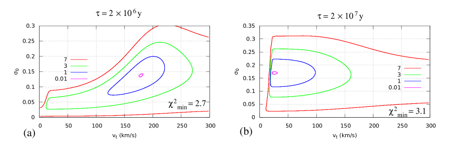
Figure 5: Contours of $\delta\chi^{2}$ in the $v_{t}$-$\sigma_{0}$ plane for excited dark matter with lifetime $\tau\sim 2\times 10^{6}\,$y (a) and $2\times 10^{7}\,$y (b), excluding Perseus data. Minimum values of $\chi^{2}$ increase by $\sim 3$ but shapes of contours do not change significantly with inclusion of Perseus cluster. $\sigma_{0}$ is in units of $10^{-22}$cm³s${}^{-1}/$(km/s)$\cdot(m_{\chi}/{\rm 10\ GeV})^{2}$.

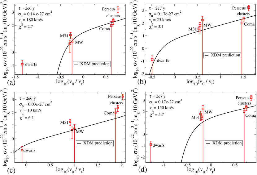
Figure 6: Data points: experimentally motivated values of the cross section (times $(10{\rm\ GeV}/m_{\chi})^{2})$ versus $v_{0}/v_{t}$ (proportional to DM velocity dispersion, $\sigma_{v}=\sqrt{3/2}\,v_{0}$). Curve is theoretical prediction of excited dark matter framework. Left (right) column is for excited state lifetime $\tau=2\times 10^{6}\,$ y ( $2\times 10^{7}\,$ y). Topmost graphs are for best-fit values of $\sigma_{0}$ and $v_{t}$ in fig. 5). Bottom graphs are for the lower or higher values of $v_{t}=10,\,150$ km/s relative to best fits (also acceptable fits), the first being marginally compatible with limit from dwarf spheroidals.

Inserting the approximate correction factors into the (numerically evaluated) integrals of $\rho^{2}/x^{2}$ for the two galaxies, we find no significant change in the predicted flux from M31 except for $\sigma=0.1\,r_{s}$, where it decreases by only a factor of 1.9. On the other hand, for $\sigma=(10^{-2},\,10^{-1})\,r_{s}$ there is a respective factor of $(18,\,300)$ reduction in the flux from the MW for the FOV of ref. Riemer-Sorensen:2014yda , requiring a corresponding increase in the upper limit for the cross section, $(0.15-1.1)\to(3-20)$ or $(40-330)$ as indicated in column 5 of table 1. For the FOV of ref. Boyarsky:2014ska , the reduction is a factor of $(12,\,200)$ respectively, leading to the replacement $(0.1-0.7)\to(2-12)$ or $(20-130)$ in the allowed values of $\langle\sigma v\rangle$. For streaming lengths $\sigma$ closer to $0.01\,r_{s}$ the target values of $\langle\sigma v\rangle$ become comparable for M31 and MW, as would be expected for two such similar galaxies, while the range of upper limits is also compatible with these detections. On the other hand, fluxes from clusters should be unchanged due to the much smaller value of $\sigma/r_{s}$ in those much larger systems. Similarly, galaxy limits of ref. Anderson:2014tza and Malyshev:2014xqa are unchanged since the FOVs cover a much greater fraction of $r_{s}$ than for the MW observation. Streaming lengths $\sigma\lesssim 10^{-3}\,r_{s}$ are too short to make any difference for the MW fluxes.

We do not attempt a more quantitative fit of the smearing length here, in light of the large uncertainties in the desired cross section values. The approximate lifetime needed for the excited state is $\tau\sim\sigma/\sigma_{v}\cong(0.2,\,2)\,$kpc/(100 km/s) $\cong 2\times 10^{6}\,$y or $2\times 10^{7}\,$y respectively, for $\sigma=(0.01,\,0.1)\,r_{s}$. It will be seen presently that the shorter lifetime gives a somewhat better fit to the data.

To fit the resulting cross sections together with those from other systems, we need to know the velocity dispersions of the two galaxies. For the MW, data exists only down to $r\cong 10$ kpc, where estimates range from $\sigma_{v}=105$ to 130 km/s Dehnen:2006cm ; Brown:2009nh . We have adopted an average value 118 km/s. For M31, measurements exist for smaller radii $\sim 0.1\,$kpc merrett . We reproduce these measurements in fig. 3, along with our fit to the analytic form $\sigma_{v}=(57.9+108.3\,e^{-5.05\,\theta})\,$km/s, where $\theta$ is in degrees. Translating this into a radial dependence, we compute the average value $\langle\sigma_{v}\rangle=[\int d^{\,3}x\,\rho^{2}\sigma_{v}/x^{2}]/[\int d^{\,3}x\,\rho^{2}/x^{2}]$ $=116\,$km/s, where the angular part of the integrals is over the $0.22^{\circ}$ FOV. This procedure is only meaningful for estimating the effect on the cross section through eq. (12) if $v_{t}\lesssim\sqrt{2/3}\langle\sigma_{v}\rangle$; otherwise we should compute the average value of $\gamma$ in the integral rather than just $\sigma_{v}$ (for small $v_{t}$ the two are proportional). We have carried this out for the 0.22^∘ FOV and the result is shown in fig. 4.

IX.1.2 Noncuspy halo profiles

Table 1 shows that the cored Burkert profile goes too far in reducing the MW signal relative to that of M31. A dark matter profile somewhere between Burkert and NFW is needed to give maximum overlap between the desired ranges of cross sections for the two galaxies, assuming that the excited state decays promptly. An example that can interpolate between the two is the Einasto profile,

$$\rho_{E}=\rho_{s}\exp\left(-{2\over\alpha}\left[\left(r\over r_{s}\right)^{\alpha}-1\right]\right)$$ (15)

A set of standard values often used, compatible with predictions from DM-only $N$-body simulations Navarro:2008kc , is $\alpha=0.17$, $r_{s}=20\,$kpc. The concentration of DM near the center depends strongly upon $\alpha$, and we find that a large value $\alpha=0.30$ (holding $r_{s}$ fixed at 20 kpc) is required to increase the cross section for MW observations of the X-ray line by a factor of 36 while increasing that of M31 by only a factor of 2, which may be sufficient to reconcile their values within the errors. With larger $r_{s}=30\,$kpc, smaller $\alpha=0.25$ can achieve a similar effect.

The question of whether the MW halo is cuspy or cored is still debated in the literature, with some indications that including the effects of baryons leads to cuspier halo Tissera:2009cm ,Schaller:2014uwa , while others argue that cored profiles are observationally preferred Nesti:2013uwa . We consider the noncuspy possibility as one option for understanding the strength of the 3.5 keV line from the galactic center, and will use this freedom to fit it away using the unknown halo profile in part of the analysis that follows.

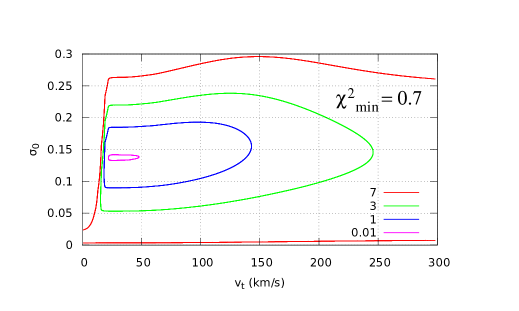
Figure 7: Similar to fig. 5 but for promptly decaying excited states, with MW contributions assumed to be fitted by adjusting the DM halo profile.

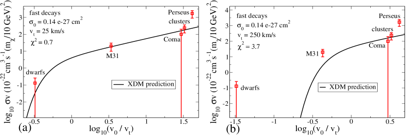
Figure 8: Similar to fig. 6 but for promptly decaying excited states, with MW contributions assumed to be fitted by adjusting the DM halo profile.

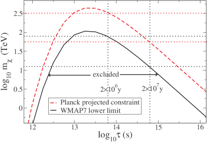
Figure 9: CMB Lower limit on DM mass $m_{\chi}$ versus lifetime of excited state, assuming relative abundance $f_{x}=1/2$ of the excited state.

IX.2 XDM parameter best fits

We proceed to search for the preferred values of the XDM model parameters $v_{t}$, the threshold velocity, and the cross section normalization $\sigma_{0}$, defined in eqs. (9,10), using the cross section values in columns 4 and 5 of table 1. We consider two cases: (1) the excited state has lifetime $\sim 10^{6}-10^{7}\,$y, and the MW has an NFW profile; (2) the excited state undergoes fast decays, and the MW halo is assumed to have the right shape for resolving the tension between MW and M31 observations of the X-ray line. In the first case we include MW data in the fit while in the second we omit them.

IX.2.1 Long-lived excited states

Starting with the intermediate lifetime scenario, recall that the values in column 4 are unchanged for sources that have no entry in column 5, and the upper (lower) entries of the latter apply for the excited state lifetime of $2\times 10^{6}(10^{7})\,$y; we consider both cases here. The predicted value of the cross section is given by eqs. (10,11) with $v_{0}=\sqrt{2/3}\,\sigma_{v}$ and $\sigma_{v}$ given in column 7 of table 1, except for M31 where we use the more quantitative averaging of $\gamma$ over the FOV as described in section IX.1 and fig. 4. As previously discussed, we do not include the measurements of the off-center Perseus cluster flux in our fits since they are not compatible with the model (nor with decaying DM models, if the dwarf spheroidal constraints are believed).

Defining a $\chi^{2}$ statistic using the cross section ranges shown in table 1 to estimate the central values and the uncertainties, we find preferred regions in the $v_{t}$-$\sigma_{0}$ plane as shown in fig. 5. The uncertainties are presently too large to justify a formal statistical analysis, so instead of showing the usual confidence intervals, steps in $\delta\chi^{2}$ of $\sim 1,\,2,\,4$ are chosen for the contours above the minimum value. The best-fit values of the threshold velocity are 180 (25) km/s for the $10^{6}(10^{7})\,$y lifetimes, respectively, not including the Perseus cluster in the fit; including it shifts these values to 186 (25) km/s. Using (9), these correspond to the range of dark matter masses $m_{\chi}\sim 80$ GeV to $4$ TeV, with $m_{\chi}$ going as $v_{t}^{-2}$. The minimum value of $\chi^{2}$ increases by approximately 3 when including Perseus on-center data in the fit, but the best-fit values do not shift significantly. The comparisons of the predictions to the data, in terms of $\langle\sigma v\rangle$ versus $v_{0}/v_{t}$, are shown in figs. 6(a,b) for these two lifetimes. The predicted signal is far below the sensitivity of spheroidal dwarf searches at low $v_{0}$ for $\tau=2\times 10^{6}\,$y, but saturating the dwarf constraint for $\tau=2\times 10^{7}\,$y.

However the minimum of $\chi^{2}$ is rather shallow and allows for larger or smaller values of $v_{t}$ to still give an acceptable fit. Thus the correlation of smaller $\tau$ with larger $v_{t}$ is not mandatory, and we display examples with the opposite behavior yet still providing acceptable fits in figs. 6(c,d), with $v_{t}$ as low as $10$ km/s, corresponding to dark matter mass $m_{\chi}=25$ TeV. Thus in either model it would be possible to start to detect the X-ray line in dwarfs given longer exposures, or for the signal from dwarfs to be far too weak for detection. The range of allowed DM masses remains as previously estimated.

IX.2.2 Fast-decaying excited states

If we assume that the MW halo has the right shape for consistency of the X-ray limits or detections from the galactic center, as we have already argued is plausible, then the MW data can be omitted from our fits, and we obtain the $\chi^{2}$ contours shown in fig. 7. The best fit parameters are similar to those in the previously considered cases of longer excited state lifetimes, and also like those cases, acceptable fits can be found at either high or low threshold velocities where dwarf spheroidals could be respectively far from or close to providing an observable strength of the X-ray line. This is illustrated in fig. 8, showing the data versus the prediction for cross section versus DM velocity. Allowing for $v_{t}$ in the range $25-300$ km/s, we find the range of dark matter masses 40 GeV to 30 TeV, with large masses corresponding to low threshold velocities.

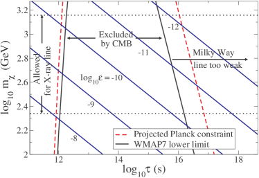
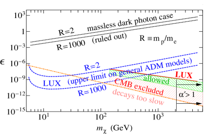
Figure 10: Left: similar to fig. 9, with diagonal lines showing contours of constant gauge kinetic mixing parameter $\epsilon$ in the atomic DM model. Right: impact of CMB constraint on region allowed by direct detection in $m_{\chi}$-$\epsilon$ plane.

IX.3 CMB constraints

There is one further experimental constraint on XDM models that must be considered when the excited state lifetime is as long as those we have investigated. Such decays in the early universe inject electromagnetic energy into the thermal plasma at a time when it can have an impact on the temperature fluctuations of the cosmic microwave background by delaying recombination, changing the optical depth, or the redshift of reionization Chen:2003gz -Diamanti:2013bia . If the lifetime is sufficiently short or long, the decays either complete before the relevant epoch or are too slow to have an appreciable effect. But for the lifetimes we have singled out as being interesting for reconciling X-ray observations of the MW galactic center with other measurements of the 3.5 keV line, decays producing photons can have a significant impact on the cosmic microwave background (CMB).

The constraints on decays are typically expressed as an upper limit on the fraction of the total DM energy density that can released into photons (or other ionizing radiation). This fraction is given by

$$f=f_{x}{\Delta E\over m_{\chi}}$$ (16)

where $f_{x}$ is the abundance of the excited state relative to the total DM abundance, and $\Delta E=3.5$ keV for the current application. An upper limit on $f$ thus translates into a lower limit on the DM mass $m_{\chi}$. We have estimated this limit for the case $f_{x}=1/2$ as a function of the excited state lifetime in fig. 9. The current hard constraint is based upon WMAP7 data, while projected constraints using Planck data await the release of Planck polarization results. We have determined these constraints using the methods described in ref. Cline:2013fm . The latter are limited to injection energies no less than $\sim 5$ GeV, while we are interested in the case of 3.5 keV. We have rescaled the constraints for the case of DM decaying into two 5 GeV photons by a factor of $8.3/2=4.2$ greater sensitivity, by reading off from fig. 6 of ref. Slatyer:2012yq the relative constraint on the lifetime as a function of deposited energy.

From fig. 9 we see that large DM masses are required, $m_{\chi}>5$ TeV, for the least constraining case of $\tau=2\times 10^{7}\,$y, using the WMAP7 data, while at $\tau=2\times 10^{6}\,$y the WMAP7 limit is $m_{\chi}>32$ TeV, both being somewhat in tension with our low-$v_{t}$ fits to the X-ray line strength, notably the limit from nonobservation in dwarf spheroidals. If the projected Planck limits are validated, then the scenario is ruled out, with the limit $m_{\chi}>55$ TeV in the longer lifetime case being incompatible with the dwarf constraints.

One must keep in mind however that these constraints would be relaxed if there is a mechanism for depleting the excited state relative abundance $f_{x}$ before the epoch of decays in the early universe. For example if the kinetic temperature of the DM becomes lower than that of the visible sector at early times, the relaxation process $\chi^{\prime}\chi^{\prime}\to\chi\chi$ can effectively deplete the excited state, before the redshifts relevant for the CMB, due to the relatively high DM density. This requires that inelastic scattering $\chi+X\to\chi^{\prime}+X$ on standard model particles $X$ go out of equilibrium at early times to prevent the repopulation of the excited state. After structure formation, following $\chi\chi\to\chi^{\prime}\chi^{\prime}$ in galaxies, the relaxation process can be slower than decays because of the smaller excited state density relative to that in the early universe.

X Models

We briefly consider the implications of our constraints for some specific models of XDM that have been previously proposed for the 3.5 keV line. In ref. Cline:2014eaa , the hyperfine transition in a model of atomic DM with kinetic mixing of the dark photon to the normal photon was suggested, in which the cross section for $\chi\chi\to\chi^{\prime}\chi^{\prime}$ was estimated to be $100\,a_{0}^{2}$, where $a_{0}$ is the Bohr radius of the dark atom. We identify this with the parameter $\sigma_{0}\cong 0.2\times 10^{-27}$cm${}^{2}(m_{\chi}/10{\rm\ GeV})^{2}$ determined from our fits in the previous section. The mass splitting $\Delta E=3.5$ keV is predicted to be $(8/3)\alpha^{\prime 4}m_{\chi}/f(R)^{2}$, where $\alpha^{\prime}$ is the dark gauge coupling, $R$ is the ratio of the dark proton to dark electron mass, and $f=R+2+1/R\geq 4$. Eliminating $\alpha^{\prime}$ from these relations, one can solve for the dark atom mass $m_{\chi}=90(f/4)^{2/7}$ GeV, smaller by a factor of $0.65$ than the estimate made in Cline:2014eaa . For perturbativity in $\alpha^{\prime}$, one requires $R<5\times 10^{4}$ hence $m_{\chi}<1.4$ TeV, while efficient recombination in the dark sector requires $R\gtrsim 100$ hence $m_{\chi}>225$ GeV. The entire range of allowed values for the DM mass in this model is therefore consistent with the current data for the line (excluding the Perseus cluster as we have discussed).

CMB constraints on the atomic XDM model were not considered in ref. Cline:2014eaa . The lifetime of the excited state is predicted to be $\tau=3m_{\chi}^{2}/(\alpha\epsilon^{2}f^{2}\Delta E^{3})$ where $\epsilon$ is the gauge kinetic mixing parameter. We illustrate the CMB constraints over the relevant mass range by plotting contours of constant $\epsilon$ over the previously shown CMB upper limit on $m_{\chi}$ as a function of $\tau$ in fig. 10(left). The regions between the dotted horizontal lines and to the left of the CMB curve are allowed. The intermediate lifetime cases $\tau\sim 2\times 10^{6}-2\times 10^{7}$y ($10^{13}-10^{15}$s) are excluded for the atomic XDM model, and longer lifetimes are disfavored by the claimed Milky Way observations since they would dilute the signal from the GC too much. We must rely upon a noncuspy halo profile in this case, as discussed in section IX.1.2. The CMB constraint significantly reduces the region of parameter space in the $m_{\chi}$-$\epsilon$ plane that is allowed by direct detection, as shown in fig. 10(right). The model can eventually be ruled out or discovered by improvements in sensitivity of direct DM searches.

A second class of realizations of XDM was provided in ref. Cline:2014kaa , where the dark sector has a broken SU(2) gauge symmetry with nonabelian kinetic mixing between one of the dark gauge boson components and the photon. In these models, the kinetic mixing parameter $\epsilon$ must be sufficiently large to get the observed X-ray line strength, leading to stronger direct detection constraints on $\epsilon$, and the necessity to demand $m_{\chi}\lesssim$ a few GeV to evade these constraints. Through eq. (9) this corresponds to large threshold velocities $v_{t}\gtrsim 1100\,$km/s that are strongly disfavored by our fits since they would suppress signals from any sources except for galaxy clusters. These models thus seem to be in conflict with the current data. It should be kept in mind however our assumption that all the significant velocity dependence in the cross section is due to the phase space. Models with very light mediators, hence an additional source of velocity dependence, require special treatment that is beyond the scope of the present work.

XI Conclusions

In this paper we have reassessed the observational claims for and against the 3.5 keV X-ray line, with emphasis on the possibility that excited dark matter models can overcome the discrepancies that decaying DM models seem to exhibit. Although the flux from the Perseus cluster is somewhat too high compared to the other sources, especially at large angles from the cluster center, the error bars for the on-center data are sufficiently large that it is possible to obtain a reasonable fit to these data, combined with stacked galaxy clusters, galaxies, M31, the galactic center, and dwarf spheroidals, within the XDM framework. While XDM does introduce a new parameter to DM models (the threshold velocity $v_{t}$), it is noteworthy that the data roughly follows the expected dependence on the DM velocity dispersion and removes the contradictory observations between low- and high-dispersion objects. In order to resolve a slight discrepancy between M31 and MW observations, it is possible to introduce another parameter, the lifetime of the excited state decay; however, it is also possible that a slightly cored DM halo for the MW resolves this discrepancy. In fact, this second option is preferred in the concrete XDM model we considered here and is well within the limits of our knowledge about the DM distribution in the MW.

Nonobservation of the line in dwarf galaxies is consistent with expectations that objects with low DM velocity dispersion should give a smaller signal from XDM. However the current data allow a large range of dark matter masses, $m_{\chi}\sim 40$ GeV $-$ 25 TeV. At the heavy extreme, the threshold velocity for producing the excited state can be sufficiently low so that dwarf spheroidals may be close to exhibiting a positive signal for the line, given longer exposures than those used so far to obtain upper limits on the flux. At the lighter end, these systems will always be orders of magnitude below the required sensitivity, whereas it is galaxies like M31 and the MW that are close to the kinematic threshold for producing the excited states. Hopefully recent proposals to observe the line more carefully will lead to clarification of the experimental situation in the near future, and enable us to better constrain this class of models.

Acknowledgments. We thank A. Boyarsky, E. Bulbul, G. Holder, D. Malyshev, G. Moore, O. Ruchayskiy, P. Scott, R. Riemer-Sørensen, T. Slatyer, O. Urban and A. Vincent for helpful discussions or correspondence. We thank J. Conlon for pointing out an error in the first version of this paper. Our work is supported by the Natural Sciences and Engineering Research Council (NSERC) of Canada.

Appendix A Profile integrals

Here we give expressions for various integrals over the DM density. The functions $h_{n}$ from eq. (4) are given by

$$h_{1} = \ln(1+c)-{c\over 1+c}$$

$$h_{2} = {\textstyle{1\over 3}}\left(1-(1+c)^{-3}\right)$$ (17)

for NFW profiles, while for the Einasto profile $\rho=\rho_{s}e^{-(2/\alpha)((r/r_{s})^{\alpha}-1)}$,

$$h_{n}={e^{2^{n}/\alpha}\over\alpha}\left(8^{-{n\over\alpha}}\,\alpha^{3\over\alpha}\,\Gamma_{\nu}\left({\textstyle{3\over\alpha}}\right)-c^{3}\,E_{1-{3\over\alpha}}\left({2^{n}\,c^{\alpha}\over\alpha}\right)\right)$$ (18)

The integrals of $\rho/x^{2}$ and $\rho^{2}/x^{2}$ over a field of view can be performed analytically for NFW profiles using two approximations. First one writes

$$\int{d^{\,3}x\over x^{2}}\rho^{n}\cong 2\pi\int_{\cos\theta_{0}}^{1}\!\!\!\!dy\int_{-\infty}^{\infty}\!\!\!dz\,\rho^{n}(\sqrt{z^{2}+d^{2}-2zyd})$$ (19)

where $\theta_{0}$ is the angular size of the observed region and $y=\cos\theta$. A small error is made by including the region behind the observer in the LOS integral; this makes the $z$ integral analytically tractable after shifting $z\to z+yd$ and completing the square so that $z^{2}+d^{2}-2zyd\to z^{2}+d^{2}(1-y^{2})=z^{2}+d^{2}\sin^{2}\theta$. Then one makes the small-angle approximation $y=1-\theta^{2}/2$ (or $\sin\theta=\theta$) and integrates with respect to $\theta$. The result is

$$\int{d^{\,3}x\over 4\pi\,x^{2}}\rho^{n}\cong{\rho_{s}^{n}r_{s}^{3}\over d^{2}}\,f_{n}(a)$$ (20)

where $a=d\theta_{0}/r_{s}$ and the dimensionless functions are given by

$$f_{1} = {\rm Re}\left[\ln(a/2)+{\ln\left((1+\sqrt{1-a^{2}})/a\right)\over(1-a^{2})^{1/2}}\right]$$

$$f_{2} = {\rm Re}\left[\frac{4-a^{2}}{6\left(a^{2}-1\right)^{2}}+{\pi a\over 2}-\frac{2}{3}\right.$$ (21)

$$- \left.\frac{\left(2a^{4}-5a^{2}+4\right)a^{2}\tanh^{-1}\left(\sqrt{1-a^{2}}\right)}{2\left(1-a^{2}\right)^{5/2}}\right]$$

The above expressions are manifestly real if $a<1$, and their analytic continuation to $a>1$ is correctly given by taking the real parts, which we find simpler than specifying the real analytic continuations explicitly.

The above treatment assumes that the field of view is centered on the object of interest. If the FOV is off-axis by an angle $\theta$ which is much larger than the opening angle of the FOV, then the above treatment is modified; instead of integrating over $\theta$ (and the azimuthal angle), one simply multiplies by the solid angle $\delta\Omega$ of the FOV. In this case we obtain

$$\int{d^{\,3}x\over 4\pi\,x^{2}}\rho^{n}\cong{\rho_{s}^{n}\,r_{s}}\,{\delta\Omega\over 4\pi}\,g_{n}(a)$$ (22)

where $a=d\sin\theta/r_{s}$ and

$$g_{1} = {\ln\left((1+\sqrt{1-a^{2}})/a\right)\over(1-a^{2})^{3/2}}-(1-a^{2})^{-1/2}$$

$$g_{2} = {-6a^{7}+23a^{5}-43a^{3}+26a\over 6a\left(1-a^{2}\right)^{4}}+{\pi\over 2a}$$

$$+ {\left(2a^{6}-7a^{4}+8a^{2}-8\right)\tanh^{-1}\left(\sqrt{1-a^{2}}\right)\over 2(1-a^{2})^{7/2}}$$

References

- (1) E. Bulbul, M. Markevitch, A. Foster, R. K. Smith, M. Loewenstein and S. W. Randall, Astrophys. J. 789, 13 (2014) [arXiv:1402.2301 [astro-ph.CO]].
- (2) A. Boyarsky, O. Ruchayskiy, D. Iakubovskyi and J. Franse, arXiv:1402.4119 [astro-ph.CO].
- (3) S. Riemer-Sørensen, arXiv:1405.7943 [astro-ph.CO].
- (4) A. Boyarsky, J. Franse, D. Iakubovskyi and O. Ruchayskiy, arXiv:1408.2503 [astro-ph.CO].
- (5) M. E. Anderson, E. Churazov and J. N. Bregman, arXiv:1408.4115 [astro-ph.HE].
- (6) D. Malyshev, A. Neronov and D. Eckert, arXiv:1408.3531 [astro-ph.HE].
- (7) A. Boyarsky, D. Iakubovskyi and O. Ruchayskiy, Phys. Dark Univ. 1, 136 (2012) [arXiv:1306.4954 [astro-ph.CO]].
- (8) O. Urban, N. Werner, S. W. Allen, A. Simionescu, J. S. Kaastra and L. E. Strigari, arXiv:1411.0050 [astro-ph.CO].
- (9) T. E. Jeltema and S. Profumo, arXiv:1408.1699 [astro-ph.HE].
- (10) A. Boyarsky, J. Franse, D. Iakubovskyi and O. Ruchayskiy, arXiv:1408.4388 [astro-ph.CO].
- (11) E. Bulbul, M. Markevitch, A. R. Foster, R. K. Smith, M. Loewenstein and S. W. Randall, arXiv:1409.4143 [astro-ph.HE].
- (12) D. Iakubovskyi, arXiv:1410.2852 [astro-ph.HE].
- (13) D. P. Finkbeiner and N. Weiner, Phys. Rev. D 76, 083519 (2007) [astro-ph/0702587].
- (14) M. Pospelov and A. Ritz, Phys. Lett. B 651, 208 (2007) [hep-ph/0703128 [HEP-PH]].
- (15) D. P. Finkbeiner and N. Weiner, arXiv:1402.6671 [hep-ph].
- (16) M. T. Frandsen, F. Sannino, I. M. Shoemaker and O. Svendsen, JCAP 1405, 033 (2014) [arXiv:1403.1570 [hep-ph]].
- (17) J. M. Cline, Y. Farzan, Z. Liu, G. D. Moore and W. Xue, Phys. Rev. D 89, 121302 (2014) [arXiv:1404.3729 [hep-ph]].
- (18) J. M. Cline and A. R. Frey, arXiv:1408.0233 [hep-ph].
- (19) A. Boyarsky, A. Neronov, O. Ruchayskiy and M. Shaposhnikov, Mon. Not. Roy. Astron. Soc. 370, 213 (2006) [astro-ph/0512509].
- (20) Vikhlinin, A., Kravtsov, A., Forman, W., et al. 2006, ApJ, 640, 691
- (21) M. Girardi, D. Fadda, G. Giuricin, F. Mardirossian, M. Mezzetti and A. Biviano, Astrophys. J. 457, 61 (1996) [astro-ph/9507031].
- (22) E.T. Million, S.W. Allen, N. Werner, G.B. Taylor, Mon. Not. Roy. Astron. Soc. 405, 1624 (2010)
- (23) E. Corbelli, S. Lorenzoni, R. A. M. Walterbos, R. Braun and D. A. Thilker, Astron. Astrophys. 511, A89 (2010) [arXiv:0912.4133 [astro-ph.CO]].
- (24) J.I. Read, Journal of Physics G Nuclear Physics, 41, 063101 (2014) [arXiv:1404.1938 [astro-ph.GA]].
- (25) F. Nesti and P. Salucci, JCAP 1307, 016 (2013) [arXiv:1304.5127 [astro-ph.GA]].
- (26) A. Klypin, H. Zhao, and R.S. Somerville, Ap.J. 573, 597 (2002), astro-ph/0110390.
- (27) E. Tempel, A. Tamm and P. Tenjes, [arXiv:0707.4374 [astro-ph]].
- (28) A. Simionescu, S. W. Allen, A. Mantz, N. Werner, Y. Takei, R. G. Morris, A. C. Fabian and J. S. Sanders et al., Science 331, 1576 (2011) [arXiv:1102.2429 [astro-ph.CO]].
- (29) M. Cicoli, J. P. Conlon, M. C. D. Marsh and M. Rummel, Phys. Rev. D 90, 023540 (2014) [arXiv:1403.2370 [hep-ph]].
- (30) B. Rasheed, N. Bahcall and P. Bode, Proc. Nat. Acad. Sci. - PNAS , 108, 3487 (2011), arXiv:1007.1980 [astro-ph.CO].
- (31) E. Bulbul, private communication
- (32) D. J. Horner, R. F. Mushotzky and C. A. Scharf, Astrophys. J. 520, 78 (1999) [astro-ph/9902151].
- (33) M. Arnaud, E. Pointecouteau and G. W. Pratt, Astron. Astrophys. 441, 893 (2005) [astro-ph/0502210].
- (34) M. G. Walker, M. Mateo, E. W. Olszewski, J. Penarrubia, N. W. Evans and G. Gilmore, Astrophys. J. 704, 1274 (2009) [Erratum-ibid. 710, 886 (2010)] [arXiv:0906.0341 [astro-ph.CO]].
- (35) F. Prada, A. A. Klypin, A. J. Cuesta, J. E. Betancort-Rijo and J. Primack, Mon. Not. Roy. Astron. Soc. 428, 3018 (2012) [arXiv:1104.5130 [astro-ph.CO]].
- (36) M.F. Struble, H.J. Rood, Astrophys. J. 125, 35 (1999)
- (37) W. Dehnen, D. McLaughlin and J. Sachania, Mon. Not. Roy. Astron. Soc. 369, 1688 (2006) [astro-ph/0603825].
- (38) W. R. Brown, M. J. Geller, S. J. Kenyon and A. Diaferio, Astrophys. J. 139, 59 (2010) arXiv:0910.2242 [astro-ph.GA].
- (39) H.R. Merrett,, M.R. Merrifield, N.G. Douglas, et al. Mon. Not. Roy. Astron. Soc. 369, 120 (2006)
- (40) J. F. Navarro, A. Ludlow, V. Springel, J. Wang, M. Vogelsberger, S. D. M. White, A. Jenkins and C. S. Frenk et al., arXiv:0810.1522 [astro-ph].
- (41) P. B. Tissera, S. D. M. White, S. Pedrosa and C. Scannapieco, Mon. Not. Roy. Astron. Soc. 406, 922 (2010) [arXiv:0911.2316 [astro-ph.CO]].
- (42) M. Schaller, C. S. Frenk, R. G. Bower, T. Theuns, A. Jenkins, J. Schaye, R. A. Crain and M. Furlong et al., arXiv:1409.8617 [astro-ph.CO].
- (43) X. L. Chen and M. Kamionkowski, Phys. Rev. D 70, 043502 (2004) [astro-ph/0310473].
- (44) D. P. Finkbeiner, S. Galli, T. Lin and T. R. Slatyer, Phys. Rev. D 85, 043522 (2012) [arXiv:1109.6322 [astro-ph.CO]].
- (45) T. R. Slatyer, Phys. Rev. D 87, no. 12, 123513 (2013) [arXiv:1211.0283 [astro-ph.CO]].
- (46) J. M. Cline and P. Scott, JCAP 1303, 044 (2013) [Erratum-ibid. 1305, E01 (2013)] [arXiv:1301.5908 [astro-ph.CO]].
- (47) R. Diamanti, L. Lopez-Honorez, O. Mena, S. Palomares-Ruiz and A. C. Vincent, JCAP 1402, 017 (2014) [arXiv:1308.2578 [astro-ph.CO]].