Brief Review of Saturation Physics

Abstract

We present a short overview of saturation physics followed by a summary of the recent progress in our understanding of nonlinear small-$x$ evolution. Topics include McLerran–Venugopalan model, Glauber–Mueller approximation, nonlinear BK/JIMWLK evolution equations, along with the running-coupling and NLO corrections to these equations. We conclude with selected topics in saturation phenomenology.

12.38.-t, 12.38.Bx, 12.38.Cy, 12.38.Mh

1 Introduction

Saturation physics is built on an observation that small Bjorken-$x$ part of the wave function for an ultrarelativistic hadron or nucleus contains an intrinsic hard scale, the saturation scale $Q_{s}$ [1]. This scale characterizes the typical size of color charge density fluctuations in the small-$x$ wave functions [2, 3, 4]. The number of partons in the proton or nuclear wave function grows at small-$x$, as shown in Fig. 1, leading to a high density of quarks and gluons inside the proton. This high density leads to large color charge fluctuations, and, therefore, to a large value of $Q_{s}$.

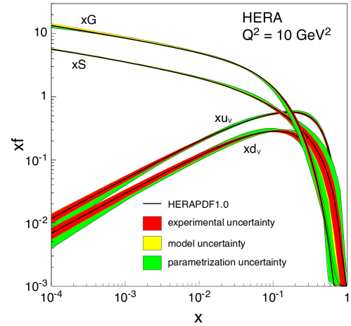
Figure 1: Parton distribution functions (PDFs) of a proton at the scale $Q^{2}=10$ GeV² plotted as functions of Bjorken $x$. Here $xu_{v}$ and $xd_{v}$ are the valence quark distributions, $xS$ is the sea quark distribution, and $xG$ is the gluon distribution. Note that the vertical axis is logarithmic.

In fact, a detailed calculation shows that the saturation scale grows as

$$Q_{s}^{2}\sim A^{1/3}\,\left(\frac{1}{x}\right)^{\lambda},$$ (1)

where $A$ is the atomic number of the nucleus. The numerical value of the inverse power of Bjorken-$x$ is approximately $\lambda\approx 0.2-0.3$. From Eq. (1) we conclude that at small enough value of $x$ and/or for large enough nucleus the saturation scale $Q_{s}$ becomes larger than the QCD confinement scale $\Lambda_{QCD}$, $Q_{s}\gg\Lambda_{QCD}$ such that the strong coupling constant becomes small,

$$\alpha_{s}(Q_{s}^{2})\ll 1.$$ (2)

Therefore, in the saturation regime we are dealing with a high density of gluons and quarks inside the proton or nucleus, while at the same time having a small coupling constant justifying the use of perturbative expansion in the powers of $\alpha_{s}$.

2 Classical Gluon Fields

The most convenient system to study saturation dynamics appears to be the small-$x$ wave function of a large nucleus. From now one we will concentrate on gluons, since they dominate over quarks at small-$x$ as follows from Fig. 1. The small-$x$ gluons “see” the whole nucleus coherently in the longitudinal direction, and can be emitted by any of the nucleons at a given impact parameter. (Note that a gluon with $k_{T}\gg\Lambda_{QCD}$ is localized in the transverse coordinate space and does not interact with the nucleons at other impact parameters.) The small-$x$ gluon can originate in any of the $\sim A^{1/3}$ nucleons at a given transverse position. If the nucleus is ultrarelativistic this means that the gluon is emitted by the effective color charge density which is enhanced by a factor of $A^{1/3}$ compared to that in a single proton. This is illustrated in Fig. 2.

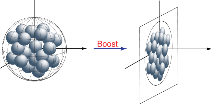
Figure 2: An ultrarelativistic nucleus appears as a “pancake” with the $A^{1/3}$-enhanced color charge density.

If we define the saturation scale squared as the gluon density in the transverse plane, one readily obtains $Q_{s}^{2}\sim A^{1/3}$, such that for a large nucleus $Q_{s}\gg\Lambda_{QCD}$ and $\alpha_{s}(Q_{s}^{2})\ll 1$. At small coupling the leading gluon field is classical (since one can neglect quantum loop corrections): hence, to find the gluon field of a nucleus one has to solve classical Yang-Mills equations

$${\cal D}_{\mu}F^{\mu\nu}=J^{\nu}$$ (3)

with the nucleus providing the source current $J^{\nu}$. This is the main concept behind the McLerran–Venugopalan model [2, 3, 4].

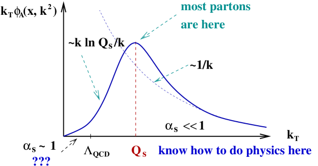
Figure 3: Unintegrated gluon distribution multiplied by the transverse momentum phase-space factor $k_{T}$ sketched as a function of $k_{T}$ (solid line). The dashed line denotes the lowest-order result, without saturation effects.

The Yang-Mills equations (3) were solved for a single nucleus source in [5, 6]. The resulting gluon field could be used to construct the unintegrated gluon distribution of a nucleus $\phi_{A}(x,k_{T}^{2})$, which counts the number of gluons at a given values of Bjorken $x$ and transverse momentum $k_{T}$:

$$\phi_{A}(x,k_{T}^{2})=\frac{C_{F}}{\alpha_{s}\,2\,\pi^{3}}\,\int d^{2}b_{\perp}\,d^{2}r_{\perp}\,e^{i{\bf k}\cdot{\bf r}}\frac{1}{r_{\perp}^{2}}\,\left[1-e^{-\frac{1}{4}\,r_{\perp}^{2}\,Q_{s}^{2}({\vec{b}}_{\perp})\,\ln(1/r_{\perp}\,\Lambda)}\right].$$ (4)

Here the gluon saturation scale is given by

$$Q_{s}^{2}({\bf b})\,=\,4\,\pi\,\alpha_{s}^{2}\,T({\bf b})$$ (5)

with $T({\bf b})$ the nuclear profile function. Transverse vectors are denoted by ${\bf x}=(x^{1},x^{2})$ and $x_{\perp}=x_{T}=|{\bf x}|$. The unintegrated gluon distribution (gluon TMD) $\phi_{A}(x,k_{T}^{2})$, multiplied by the transverse momentum phase-space factor of $k_{T}$ is plotted schematically in Fig. 3 as a function of $k_{T}$. We conclude from this plot that the majority of gluons in this classical nuclear wave function have transverse momentum $k_{T}\sim Q_{s}\gg\Lambda_{QCD}$, such that applicability of perturbation theory is justified.

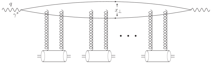
Figure 4: DIS on a large nucleus in the Glauber–Mueller approximation.

Now let us consider deep inelastic scattering (DIS) on a large nucleus, working in the same classical approximation. The DIS process at high energies is shown in Fig. 4: the electron (not shown) emits a virtual photon, which then splits into a $q\bar{q}$ pair which scatters on the nuclear target. At the lowest-order each interaction with the nucleons in the nucleus is limited to a two-gluon exchange: this is known as the Glauber–Mueller model [7]. The resummation parameter of such approximation is then $\alpha_{s}^{2}\,A^{1/3}$. It can be shown that this is also the parameter resummed by the classical gluon fields in the MV model [8].

The high-energy DIS cross section can be written as a convolution of the light-cone wave function $\Psi^{\gamma^{*}\rightarrow q{\bar{q}}}$ of the virtual photon splitting into a $q\bar{q}$ pair and the scattering amplitude of the $q\bar{q}$ on the nuclear target,

$$\sigma_{tot}^{\gamma^{*}A}(x,Q^{2})\,=\,\int\frac{d^{2}x_{\perp}}{4\,\pi}\,\int\limits_{0}^{1}\,\frac{dz}{z\,(1-z)}\ |\Psi^{\gamma^{*}\rightarrow q{\bar{q}}}({\bf x},z)|^{2}\ \sigma_{tot}^{q{\bar{q}}A}({\bf x},Y),$$ (6)

where $Y=\ln 1/x$ is the rapidity variable, $x_{\perp}$ is the transverse size of the dipole, and $z$ is the fraction of the virtual photon’s light-cone momentum carried by the quark.

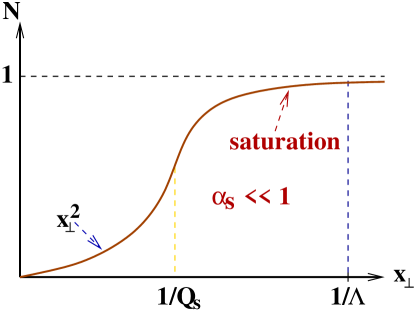
Figure 5: Dipole–nucleus forward scattering amplitude as a function of the dipole size $x_{\perp}$ in the Glauber–Mueller model.

One can write the dipole–nucleus cross section as an integral over impact parameters of the (imaginary part of the) forward dipole–nucleus scattering amplitude $N$,

$$\sigma_{tot}^{q{\bar{q}}A}({\bf x},Y)\,=\,2\,\int d^{2}b\ N({\bf x},{\bf b},Y).$$ (7)

The dipole–nucleus forward scattering amplitude is found in the Glauber–Mueller model to be [7]

$$N({\bf x},{\bf b},Y=0)\,=\,1-\exp\left\{-\frac{x_{\perp}^{2}\,Q_{sq}^{2}({\bf b})\,\ln(1/x_{\perp}\,\Lambda)}{4}\,\right\}$$ (8)

with the quark saturation scale

$$Q_{sq}^{2}({\bf b})\,\equiv\,\frac{4\,\pi\,\alpha_{s}^{2}\,C_{F}}{N_{c}}\,T({\bf b}).$$ (9)

The amplitude $N$ from Eq. (8) is sketched as a function of the dipole size $x_{\perp}$ in Fig. 5. As the dipole size goes to zero, so does the amplitude $N$. This is the manifestation of color transparency: zero-size dipole does not interact. As the dipole size increases, so does the amplitude $N$ again. However, due to multiple rescatterings effects of Fig. 4 which led to the exponentiation in Eq. (8), we always have $N<1$. Using this bound in Eq. (7) we see that, for a nucleus of radius $R$ it translates into $\sigma_{tot}^{q{\bar{q}}A}<2\pi R^{2}$, which is the well-known black disk limit. We see that saturation effects lead to the scattering cross section that preserves the black disk limit: we can invert this observation to argue that saturation is a consequence of unitarity. Note that the onset of saturation effects and the approach to the black disk regime happens around $x_{\perp}\sim 1/Q_{s}$, where the dipole is still perturbatively small and perturbation theory is applicable.

3 Small-$x$ Evolution

The classical picture presented above lacks the energy (or Bjorken-$x$) dependence. The energy-dependence enters the picture through quantum evolution corrections. The corrections for dipole–nucleus scattering in DIS are illustrated in Fig. 6. Each gluon emission brings in a power of $\alpha_{s}$ and, due to the phase-space integral, a factor of rapidity $Y$ (at the leading order). The resulting leading-logarithmic approximation (LLA) resums powers of $\alpha_{s}\,Y$.

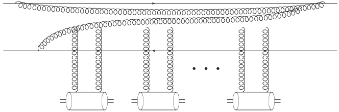
Figure 6: Small-$x$ evolution corrections to the dipole–nucleus forward scattering amplitude.

Small-$x$ evolution corrections in the large-$N_{c}$ approximation can be absorbed into the dipole amplitude $N$ with the help of the Balitsky–Kovchegov (BK) evolution equation [9, 10, 11, 12],

$$\frac{\partial}{\partial Y}\,N_{{\bf x}_{1},{\bf x}_{0}}(Y)\, = \,\frac{\alpha_{s}\,N_{c}}{2\,\pi^{2}}\,\int\,d^{2}x_{2}\,\frac{x^{2}_{10}}{x^{2}_{20}\,x^{2}_{21}}\,\bigg{[}N_{{\bf x}_{1},{\bf x}_{2}}(Y)+N_{{\bf x}_{2},{\bf x}_{0}}(Y)$$ (10)

$$- N_{{\bf x}_{1},{\bf x}_{0}}(Y)-N_{{\bf x}_{1},{\bf x}_{2}}(Y)\,N_{{\bf x}_{2},{\bf x}_{0}}(Y)\bigg{]}.$$

We have slightly modified our notation: the dipole–nucleus amplitude, now denoted by $N_{{\bf x}_{1},{\bf x}_{0}}(Y)$, depends on the positions of the quark and the anti-quark (${\bf x}_{1},{\bf x}_{0}$) in the dipole. Above $x_{ij}=|{\bf x}_{i}-{\bf x}_{j}|$. The initial condition for Eq. (10) is given by the Glauber–Mueller formula (8): this way one resums both the powers of $\alpha_{s}\,Y$ and $\alpha_{s}^{2}\,A^{1/3}$. The linear terms on the right-hand side of Eq. (10) correspond to the Balitsky–Fadin–Kuraev–Lipatov (BFKL) evolution equation [13, 14], while the quadratic term introduced damping due to saturation effects.

No closed integro-differential equation for the amplitude $N$ exists beyond the large-$N_{c}$ approximation. Instead, for general-$N_{c}$ one has to solve the Jalilian-Marian–Iancu–McLerran–Weigert–Leonidov–Kovner (JIMWLK)
evolution equation [15, 16, 17, 18], which is a functional differential equation, giving energy dependence not only for the dipole operator, but for any other operator made out of eikonal Wilson lines along the light-cone. Interestingly enough, a numerical solution of both the BK and JIMWLK evolution equations in [19, 20] indicates that the differences between the large-$N_{c}$ and any-$N_{c}$ expressions for the dipole amplitude $N$ are very small, on the order of $0.1\%$, much smaller than the naively anticipated $1/N_{c}^{2}\approx 0.1$.

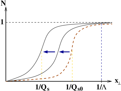
Figure 7: A sketch of the small-$x$ evolution of the dipole amplitude $N$: the initial condition (given by the Glauber-Mueller formula) is shown by the dashed line. As rapidity increases the dipole amplitude shifts to the smaller values of $x_{\perp}$ in the plot, as indicated by the solid-line curves and the arrows.

No exact analytic solution of Eq. (10) exists. Our understanding of its solution stems from several approximate analytic solutions [1, 21, 22, 23] along with the exact numerical solutions [24, 25, 26, 27]. Qualitative behavior of the solution of Eq. (10) is shown in Fig. 7. There we see that small-$x$ evolution makes the dipole amplitude shift left from the initial conditions (dashed curve), toward the smaller values of the dipole size $x_{\perp}$. The two evolved curves are shown by solid lines, with the direction of rapidity increase denoted by arrows. We see two important features in this solution. One is that we always have $N<1$: indeed $N=1$ is the fixed point of the evolution (10), such that the black disk limit is always preserved by the nonlinear evolution. Hence nonlinear small-$x$ evolution is unitary! Another feature is that the saturation scale, as the characteristic of the transition into the saturation region, is growing with rapidity: in Fig. 7 we clearly have $Q_{s}>Q_{s0}$ with $Q_{s0}$ the initial value of the saturation scale. A more careful analysis leads to $Q_{s}^{2}\sim(1/x)^{\lambda}\sim e^{\lambda\,Y}$ scaling of the saturation scale with decreasing Bjorken $x$ or increasing rapidity, justifying the claim we made in Eq. (1). The solution of the BK/JIMWLK evolution for the dipole amplitude has another important property known as the geometric scaling [28]: the dipole amplitude turns out to be a function of only one variable, $N(x_{\perp},Y)=N(x_{\perp}\,Q_{s}(Y))$, over a broad range of the dipole sizes $x_{\perp}$ [1, 21, 23].

We summarize this discussion of the nonlinear small-$x$ evolution with a map of high-energy QCD in Fig. 8.

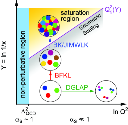
Figure 8: A map of high-energy QCD.

There we plot the action of the QCD evolution equations in the $(\ln Q^{2},\ln 1/x)$ plane. The DGLAP evolution equation, implementing renormalization group flow, evolves PDF toward large $Q^{2}$ with approximately fixed values of $x$. The linear BFKL evolution equation evolves the unintegrated gluon distribution (or dipole amplitude) toward low-$x$, but eventually stops being applicable due to violation of unitarity. The nonlinear BK/JIMWLK equations take over the BFKL evolution at low-$x$ preventing the unitarity violation and guiding the system into the saturation region.

For much more detailed presentations of saturation physics we recommend the review articles [1, 29, 30, 31, 32, 33] along with the book [34].

4 Higher-Order Corrections to the BK and JIMWLK Evolution Equations

Over the past decade, main progress in our understanding of nonlinear small-$x$ evolution came from calculation of higher-order corrections to it, and from successful phenomenological applications of the results of those calculations.

The first development in this direction was the calculation of the running-coupling correction to the BK and JIMWLK evolution equations in [35, 36, 37] using the BLM method [38]. The result, in the scheme used in [37], reads

$$\frac{\partial N_{{\bf x}_{0},{\bf x}_{1}}(Y)}{\partial Y}\,=\,\frac{N_{c}}{2\pi^{2}}\,\int d^{2}x_{2}$$

$$\times\left[\alpha_{s}\left(\frac{1}{x_{20}^{2}}\right)\,\frac{1}{x_{20}^{2}}-2\,\frac{\alpha_{s}\left(\frac{1}{x_{20}^{2}}\right)\ \alpha_{s}\left(\frac{1}{x_{21}^{2}}\right)}{\alpha_{s}\left(\frac{1}{R^{2}}\right)}\,\frac{{\bf x}_{20}\cdot{\bf x}_{21}}{x_{20}^{2}\,x_{21}^{2}}+\alpha_{s}\left(\frac{1}{x_{21}^{2}}\right)\,\frac{1}{x_{21}^{2}}\right]$$

$$\times\,\left[N_{{\bf x}_{0},{\bf x}_{2}}(Y)+N_{{\bf x}_{2},{\bf x}_{1}}(Y)-N_{{\bf x}_{0},{\bf x}_{1}}(Y)-N_{{\bf x}_{0},{\bf x}_{2}}(Y)\,N_{{\bf x}_{2},{\bf x}_{1}}(Y)\right],$$ (11)

with the scale $R$ given by

$$R^{2}({\bf x}_{0},{\bf x}_{1};{\bf z}) =\,|{\bf z}-{\bf x}_{0}|\,|{\bf z}-{\bf x}_{1}|$$

$$\times \!\!\!\!\left(\frac{|{\bf z}-{\bf x}_{1}|}{|{\bf z}-{\bf x}_{0}|}\right)^{\frac{({\bf z}-{\bf x}_{0})^{2}+({\bf z}-{\bf x}_{1})^{2}}{({\bf z}-{\bf x}_{0})^{2}-({\bf z}-{\bf x}_{1})^{2}}-2\,\frac{|{\bf z}-{\bf x}_{0}|^{2}\,|{\bf z}-{\bf x}_{1}|^{2}}{({\bf z}-{\bf x}_{0})\cdot({\bf z}-{\bf x}_{1})}\,\frac{1}{|{\bf z}-{\bf x}_{0}|^{2}-|{\bf z}-{\bf x}_{1}|^{2}}}.$$ (12)

We will refer to the BK evolution equation with running coupling corrections as rcBK. The effect of the running-coupling corrections on the small-$x$ evolution is to suppress the contribution from the very small dipoles (due to asymptotic freedom), thus slowing down the evolution. In fact the parameter $\lambda$ in Eq. (1) goes from being about $0.7-0.8$ at fixed QCD coupling down to about $0.2-0.3$ when the running coupling corrections are included [27, 39, 40]: this is a positive development, since $\lambda\approx 0.2-0.3$ gives us the energy dependence close to that observed in experimental data.

More recently, the full next-to-leading order (NLO) correction to the BK evolution kernel was calculated in a formidable calculation presented in [41]. (Running-coupling evolution of Eq. (4) contains a subset of NLO and higher-order corrections, but is not a complete NLO or higher-order result.) Knowledge of NLO BK corrections is an important part of theoretical progress in the field. Solution of the NLO BK evolution (analytical or, more likely, numerical) has not been constructed at the time of writing.

NLO corrections for the JIMWLK kernel were obtained very recently in [42, 43, 44]. Similar to BK evolution, the impact of the NLO JIMWLK corrections on the evolution of Wilson line correlators is yet to be determined.

NLO correction to the BK or JIMWLK evolution kernel is order-$\alpha_{s}^{2}$. If one solves NLO BK/JIMWLK evolution equation exactly, one would be resumming powers of $\alpha_{s}^{2}\,Y$, in addition to the powers of $\alpha_{s}\,Y$ resummed to all orders by the LLA evolution. Here one runs into the standard power-counting conundrum: two iterations of NLO evolution kernel give a contribution of the order $(\alpha_{s}^{2}\,Y)^{2}$, which is of the same order as one iteration of the leading-order (LO) kernel times an iteration of the next-to-next-to-leading order (NNLO) kernel, $(\alpha_{s}\,Y)\,(\alpha_{s}^{3}\,Y)$. It is thus a priori not clear whether construction of an all-order solution of the NLO non-linear evolution equation is parametrically justified, or whether this would overstep the precision of the approximation. Perhaps knowledge of the overall structure of the solution would facilitate this perturbative expansion (e.g. in DGLAP evolution all perturbative expansion resides in one place in the solution — the anomalous dimensions): while such program has recently been initiated for the linear BFKL evolution [45], it would be much harder to do for the nonlinear evolution case, where we do not know the exact analytic solution even in the LLA.

Figure 9: Data on DIS $\gamma^{*}+p$ total cross section for $x<0.01$ plotted as a function of $\tau=Q^{2}/Q_{s}^{2}(x)$ [28].

5 Some Saturation Phenomenology

The field of phenomenological applications of saturation physics has grown tremendously over the last decade, encompassing scattering processes as diverse as DIS, $p+p$, $p+A$ and heavy ion collisions (see [33] for an up-to-date review of saturation phenomenology). It is impossible to do full justice to this area in this short review. Instead we will only present a few phenomenological successes of saturation physics.

As discussed above, geometric scaling is a consequence of non-linear small-$x$ evolution. In Fig. 9 from [28] we show a compilation of DIS total cross section data for $x<10^{-2}$ plotted as a function of the single scaling variable $\tau=Q^{2}/Q_{s}^{2}(x)$. The figure demonstrates that small-$x$ DIS data appears to exhibit geometric scaling predicted by saturation theory [1, 21, 23]!

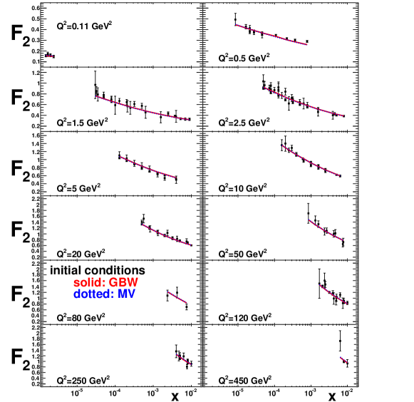
Figure 10: Fit to the HERA DIS data on $F_{2}$ structure function of the proton at low-$x$ within the saturation framework performed in [46] based on the rcBK evolution equation.

A more quantitative comparison of small-$x$ DIS data and saturation theory from [46, 47] is shown in Fig. 10 for the $F_{2}$ structure function of the proton. The theory curves shown are generated using rcBK evolution equation (employing equations like (6) and (7) to obtain the structure function). Clearly the description of the data is very good.

Saturation physics and nonlinear small-$x$ evolution are relevant not only to DIS, but to any high-energy scattering process. They are likely to play an important role in describing particle production and correlations originating in the early stages of heavy ion collisions. Description of heavy ion collisions in the saturation framework starts with determining classical gluon field of the colliding ions in the MV model. One has to solve the same Eq. (3), but now with the source given by two colliding nuclei. This problem is very hard to solve analytically, allowing only for either perturbative or variational solutions [48, 49, 50, 51, 52, 53]. Luckily the problem can be solved numerically [54, 55, 56]. Once the classical gluon production is understood, one needs to include quantum evolution corrections into the obtained formula: at present this is impossible to do analytically, though it is doable numerically [57]. The program is similar to what was done for DIS: quasi-classical Glauber–Mueller formula received quantum evolution corrections through the BK/JIMWLK equations.

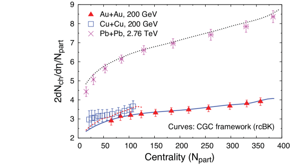
Figure 11: Saturation description of the charged hadron multiplicity in heavy ion collisions based on the KLN-type model with rcBK evolution [58]. RHIC data (Au+Au and Cu+Cu) was fitted (solid and lower dashed lines), while the LHC results (Pb+Pb) were predicted by the top dotted curve.

While the exact saturation calculation for gluon production in heavy ion collisions is rather hard to do, one could use an approximate Kharzeev–Levin–Nardi (KLN) approach [59, 60, 61] which employs the (slightly modified) $k_{T}$-factorization formula which is an exact saturation-physics result for gluon production in $p+A$ collisions [62, 63]. The unintegrated gluon distributions entering the $k_{T}$-factorization formula can be found using rcBK-evolved expression for the dipole amplitude. The result of applying this procedure to charged hadron production in $A+A$ collisions is shown in Fig. 11: while the description of RHIC data in this figure is a result of a fit, the dashed curve for the LHC is a prediction, appearing to be in a very good agreement with the data. Once again saturation physics appears to be consistent with the data, and this time it was in fact able to predict the data.

6 Outlook

While tantalizing evidence for saturation regime was seen in $e+p$, $p+A$ and $A+A$ collisions, the decisive evidence for saturation sealing the discovery case can be found at an $e+A$ collider. In high-energy $e+A$ collisions the saturation scale (1) would get enhancements from both the low value of $x$ and the large value of $A$, making the saturation region much broader than in $e+p$ collisions. Another advantage of $e+A$ collisions is a clean electron probe, allowing for higher precision in theoretical predictions and, with varying virtuality of the photon $Q^{2}$, providing an extra lever for experimental measurements, giving $e+A$ collisions an advantage over $p+A$ and $A+A$ collisions in terms of its potential for saturation discovery. An Electron Ion Collider (EIC) is being proposed in the US: for more details on the proposal we refer the reader to the EIC White Paper [64].

References

- [1] L. V. Gribov, E. M. Levin, and M. G. Ryskin, Semihard Processes in QCD, Phys. Rept. 100 (1983) 1–150.
- [2] L. D. McLerran and R. Venugopalan, Gluon distribution functions for very large nuclei at small transverse momentum, Phys. Rev. D49 (1994) 3352–3355, [hep-ph/9311205].
- [3] L. D. McLerran and R. Venugopalan, Computing quark and gluon distribution functions for very large nuclei, Phys. Rev. D49 (1994) 2233–2241, [hep-ph/9309289].
- [4] L. D. McLerran and R. Venugopalan, Green’s functions in the color field of a large nucleus, Phys. Rev. D50 (1994) 2225–2233, [hep-ph/9402335].
- [5] Y. V. Kovchegov, Non-abelian Weizsäcker-Williams field and a two- dimensional effective color charge density for a very large nucleus, Phys. Rev. D54 (1996) 5463–5469, [hep-ph/9605446].
- [6] J. Jalilian-Marian, A. Kovner, L. D. McLerran, and H. Weigert, The intrinsic glue distribution at very small x, Phys. Rev. D55 (1997) 5414–5428, [hep-ph/9606337].
- [7] A. H. Mueller, Small x Behavior and Parton Saturation: A QCD Model, Nucl. Phys. B335 (1990) 115.
- [8] Y. V. Kovchegov, Quantum structure of the non-Abelian Weizsäcker-Williams field for a very large nucleus, Phys. Rev. D55 (1997) 5445–5455, [hep-ph/9701229].
- [9] I. Balitsky, Operator expansion for high-energy scattering, Nucl. Phys. B463 (1996) 99–160, [hep-ph/9509348].
- [10] I. Balitsky, Factorization and high-energy effective action, Phys. Rev. D60 (1999) 014020, [hep-ph/9812311].
- [11] Y. V. Kovchegov, Small-x structure function of a nucleus including multiple pomeron exchanges, Phys. Rev. D60 (1999) 034008, [hep-ph/9901281].
- [12] Y. V. Kovchegov, Unitarization of the BFKL pomeron on a nucleus, Phys. Rev. D61 (2000) 074018, [hep-ph/9905214].
- [13] E. A. Kuraev, L. N. Lipatov, and V. S. Fadin, The Pomeranchuk singularity in non-Abelian gauge theories, Sov. Phys. JETP 45 (1977) 199–204.
- [14] I. Balitsky and L. Lipatov, The Pomeranchuk Singularity in Quantum Chromodynamics, Sov.J.Nucl.Phys. 28 (1978) 822–829.
- [15] J. Jalilian-Marian, A. Kovner, and H. Weigert, The Wilson renormalization group for low x physics: Gluon evolution at finite parton density, Phys. Rev. D59 (1998) 014015, [hep-ph/9709432].
- [16] J. Jalilian-Marian, A. Kovner, A. Leonidov, and H. Weigert, The Wilson renormalization group for low x physics: Towards the high density regime, Phys. Rev. D59 (1998) 014014, [hep-ph/9706377].
- [17] E. Iancu, A. Leonidov, and L. D. McLerran, The renormalization group equation for the color glass condensate, Phys. Lett. B510 (2001) 133–144.
- [18] E. Iancu, A. Leonidov, and L. D. McLerran, Nonlinear gluon evolution in the color glass condensate. I, Nucl. Phys. A692 (2001) 583–645, [hep-ph/0011241].
- [19] K. Rummukainen and H. Weigert, Universal features of JIMWLK and BK evolution at small , Nucl. Phys. A739 (2004) 183–226, [hep-ph/0309306].
- [20] Y. V. Kovchegov, J. Kuokkanen, K. Rummukainen, and H. Weigert, Subleading- corrections in non-linear small- evolution, Nucl. Phys. A823 (2009) 47–82, [arXiv:0812.3238].
- [21] E. Iancu, K. Itakura, and L. McLerran, Geometric scaling above the saturation scale, Nucl. Phys. A708 (2002) 327–352, [hep-ph/0203137].
- [22] A. H. Mueller and D. N. Triantafyllopoulos, The energy dependence of the saturation momentum, Nucl. Phys. B640 (2002) 331–350, [hep-ph/0205167].
- [23] E. Levin and K. Tuchin, Solution to the evolution equation for high parton density QCD, Nucl. Phys. B573 (2000) 833–852, [hep-ph/9908317].
- [24] K. Golec-Biernat, L. Motyka, and A. M. Stasto, Diffusion into infra-red and unitarization of the BFKL pomeron, Phys. Rev. D65 (2002) 074037, [hep-ph/0110325].
- [25] M. Braun, Structure function of the nucleus in the perturbative QCD with (BFKL pomeron fan diagrams), Eur. Phys. J. C16 (2000) 337–347, [hep-ph/0001268].
- [26] E. Levin and M. Lublinsky, Parton densities and saturation scale from non-linear evolution in dis on nuclei, Nucl. Phys. A696 (2001) 833–850, [hep-ph/0104108].
- [27] J. L. Albacete, N. Armesto, J. G. Milhano, C. A. Salgado, and U. A. Wiedemann, Numerical analysis of the Balitsky-Kovchegov equation with running coupling: Dependence of the saturation scale on nuclear size and rapidity, Phys. Rev. D71 (2005) 014003, [hep-ph/0408216].
- [28] A. M. Stasto, K. Golec-Biernat, and J. Kwiecinski, Geometric scaling for the total cross-section in the low x region, Phys. Rev. Lett. 86 (2001) 596–599, [hep-ph/0007192].
- [29] E. Iancu and R. Venugopalan, The color glass condensate and high energy scattering in QCD, hep-ph/0303204.
- [30] J. Jalilian-Marian and Y. V. Kovchegov, Saturation physics and deuteron gold collisions at RHIC, Prog. Part. Nucl. Phys. 56 (2006) 104–231, [hep-ph/0505052].
- [31] H. Weigert, Evolution at small : The Color Glass Condensate, Prog. Part. Nucl. Phys. 55 (2005) 461–565, [hep-ph/0501087].
- [32] F. Gelis, E. Iancu, J. Jalilian-Marian, and R. Venugopalan, The Color Glass Condensate, Ann.Rev.Nucl.Part.Sci. 60 (2010) 463–489, [arXiv:1002.0333].
- [33] J. L. Albacete and C. Marquet, Gluon saturation and initial conditions for relativistic heavy ion collisions, Prog.Part.Nucl.Phys. 76 (2014) 1–42, [arXiv:1401.4866].
- [34] Y. V. Kovchegov and E. Levin, Quantum Chromodynamics at High Energy. Cambridge University Press, 2012.
- [35] E. Gardi, J. Kuokkanen, K. Rummukainen, and H. Weigert, Running coupling and power corrections in nonlinear evolution at the high-energy limit, Nucl. Phys. A784 (2007) 282–340, [hep-ph/0609087].
- [36] I. I. Balitsky, Quark Contribution to the Small- Evolution of Color Dipole, Phys. Rev. D 75 (2007) 014001, [hep-ph/0609105].
- [37] Y. Kovchegov and H. Weigert, Triumvirate of Running Couplings in Small- Evolution, Nucl. Phys. A 784 (2007) 188–226, [hep-ph/0609090].
- [38] S. J. Brodsky, G. P. Lepage, and P. B. Mackenzie, On the elimination of scale ambiguities in perturbative quantum chromodynamics, Phys. Rev. D28 (1983) 228.
- [39] J. L. Albacete and Y. V. Kovchegov, Solving high energy evolution equation including running coupling corrections, Phys. Rev. D75 (2007) 125021, [0704.0612].
- [40] J. L. Albacete, Particle multiplicities in Lead-Lead collisions at the LHC from non-linear evolution with running coupling, Phys. Rev. Lett. 99 (2007) 262301, [0707.2545].
- [41] I. Balitsky and G. A. Chirilli, Next-to-leading order evolution of color dipoles, Phys. Rev. D77 (2008) 014019, [arXiv:0710.4330].
- [42] A. Grabovsky, On the solution to the NLO forward BFKL equation, JHEP 1309 (2013) 098, [arXiv:1307.3152].
- [43] I. Balitsky and G. A. Chirilli, Rapidity evolution of Wilson lines at the next-to-leading order, Phys.Rev. D88 (2013) 111501, [arXiv:1309.7644].
- [44] A. Kovner, M. Lublinsky, and Y. Mulian, Complete JIMWLK Evolution at NLO, arXiv:1310.0378.
- [45] G. A. Chirilli and Y. V. Kovchegov, Solution of the NLO BFKL Equation and a Strategy for Solving the All-Order BFKL Equation, JHEP 1306 (2013) 055, [arXiv:1305.1924].
- [46] J. L. Albacete, N. Armesto, J. G. Milhano, and C. A. Salgado, Non-linear QCD meets data: A global analysis of lepton- proton scattering with running coupling BK evolution, Phys. Rev. D80 (2009) 034031, [arXiv:0902.1112].
- [47] J. L. Albacete, N. Armesto, J. G. Milhano, P. Quiroga-Arias, and C. A. Salgado, AAMQS: A non-linear QCD analysis of new HERA data at small-x including heavy quarks, Eur. Phys. J. C71 (2011) 1705, [arXiv:1012.4408].
- [48] A. Kovner, L. D. McLerran, and H. Weigert, Gluon production from nonAbelian Weizsacker-Williams fields in nucleus-nucleus collisions, Phys. Rev. D52 (1995) 6231–6237, [hep-ph/9502289].
- [49] Y. V. Kovchegov and D. H. Rischke, Classical gluon radiation in ultrarelativistic nucleus nucleus collisions, Phys. Rev. C56 (1997) 1084–1094, [hep-ph/9704201].
- [50] Y. V. Kovchegov and A. H. Mueller, Gluon production in current nucleus and nucleon nucleus collisions in a quasi-classical approximation, Nucl. Phys. B529 (1998) 451–479, [hep-ph/9802440].
- [51] Y. V. Kovchegov, Classical initial conditions for ultrarelativistic heavy ion collisions, Nucl. Phys. A692 (2001) 557–582, [hep-ph/0011252].
- [52] I. Balitsky, Scattering of shock waves in QCD, Phys. Rev. D70 (2004) 114030, [hep-ph/0409314].
- [53] J. P. Blaizot, T. Lappi, and Y. Mehtar-Tani, On the gluon spectrum in the glasma, Nucl. Phys. A846 (2010) 63–82, [arXiv:1005.0955].
- [54] A. Krasnitz and R. Venugopalan, The initial energy density of gluons produced in very high energy nuclear collisions, Phys. Rev. Lett. 84 (2000) 4309–4312, [hep-ph/9909203].
- [55] A. Krasnitz, Y. Nara, and R. Venugopalan, Probing a color glass condensate in high energy heavy ion collisions, Braz. J. Phys. 33 (2003) 223–230.
- [56] T. Lappi, Production of gluons in the classical field model for heavy ion collisions, Phys. Rev. C67 (2003) 054903, [hep-ph/0303076].
- [57] F. Gelis, T. Lappi, and R. Venugopalan, High energy factorization in nucleus-nucleus collisions. 3. Long range rapidity correlations, Phys.Rev. D79 (2009) 094017, [arXiv:0810.4829].
- [58] J. L. Albacete and A. Dumitru, A model for gluon production in heavy-ion collisions at the LHC with rcBK unintegrated gluon densities, arXiv:1011.5161.
- [59] D. Kharzeev and E. Levin, Manifestations of high density QCD in the first RHIC data, Phys. Lett. B523 (2001) 79–87, [nucl-th/0108006].
- [60] D. Kharzeev and M. Nardi, Hadron production in nuclear collisions at RHIC and high density QCD, Phys. Lett. B507 (2001) 121–128, [nucl-th/0012025].
- [61] D. Kharzeev, E. Levin, and M. Nardi, Hadron multiplicities at the LHC, arXiv:0707.0811.
- [62] Y. V. Kovchegov and K. Tuchin, Inclusive gluon production in DIS at high parton density, Phys. Rev. D65 (2002) 074026, [hep-ph/0111362].
- [63] D. Kharzeev, Y. V. Kovchegov, and K. Tuchin, Cronin effect and high-p(t) suppression in p a collisions, Phys. Rev. D68 (2003) 094013, [hep-ph/0307037].
- [64] A. Accardi, J. Albacete, M. Anselmino, N. Armesto, E. Aschenauer, et. al., Electron Ion Collider: The Next QCD Frontier - Understanding the glue that binds us all, arXiv:1212.1701.