Conservative Anosov diffeomorphisms of $\mathbb{T}^{2}$ without an absolutely continuous invariant measure.

Abstract.

We construct examples of $C^{1}$ Anosov diffeomorphisms on $\mathbb{T}^{2}$ which are of Krieger type ${\rm III}_{1}$ with respect to Lebesgue measure. This shows that the Gurevic Oseledec phenomena that conservative $C^{1+\alpha}$ Anosov diffeomorphisms have a smooth invariant measure does not hold true in the $C^{1}$ setting.

1. Introduction

This paper provides the first examples of Anosov diffeomorphisms of $\mathbb{T}^{2}$ which are conservative and ergodic yet there is no Lebesgue absolutely continuous invariant measure.

Let $M$ be a compact, boundaryless smooth manifold and $f:M\to M$ be a diffeomorphism. A natural question which arises is whether $f$ preserves a measure which is absolutely continuous with respect to the volume measure on $M$. In order to avoid confusion in what follows, we would like to stress out that in this paper, the term conservative means the definition from ergodic theory which is non existence of wandering sets of positive measure. That is $f$ is conservative if and only for every $W\subset M$ so that $\left\{f^{n}W\right\}_{n\in\mathbb{Z}}$ are disjoint (modulo the volume measure), $vol(W)=0$.

It follows from [LS] that for a generic $C^{2}$ Anosov diffeomorphism there exists no absolutely continuous invariant measure (a.c.i.m.), [B, p. 72, Corollary 4.15.]. Following this result Sinai asked whether a generic Anosov diffeomorphism will satisfy Poincare recurrence. This question was answered by Gurevic and Oseledec [GO] who proved that the set of conservative (Poincare recurrent) $C^{2}$ Anosov diffeomorphism is meagre in the $C^{2}$ topology (restricted to the open set of Anosov diffeomorphisms). Indeed, they have proved that if $f$ is a conservative $C^{2}$ Anosov (hyperbolic) diffeomorphism, then $f$ preserves a probability measure in the measure class of the volume measure which combined with the result of Livsic and Sinai proves the non-genericity result. The proof in [GO] uses the absolute continuity of the foliations and existence of SRB measures to show that if the $SRB$ measure for $f$ is not equal to the SRB measure for $f^{-1}$ then there exists a continuous function $g:M\to\mathbb{R}$ and a set $A\subset M$ of positive volume so that,

$$\lim_{n\to\infty}\frac{1}{n}\sum_{k=0}^{n-1}g\left(f^{k}(x)\right)\neq\lim_{n\to\infty}\frac{1}{n}\sum_{k=0}^{n-1}g\left(f^{-k}(x)\right),\ \forall x\in A.$$

It is then a straightforward argument to construct a set $B\subset A$ of positive volume measure so that for almost every $x\in B$, the set $\left\{k\in\mathbb{N}:\ f^{k}x\in B\right\}$ is finite, in contradiction with Halmos Recurrence Theorem [Aar1].

This result remains true for $C^{1+\alpha},\ \alpha>0$ Anosov diffeomorphisms. However, since there exists $C^{1}$ Anosov diffeomorphisms whose stable and unstable foliations are not absolutely continuous [RY], this proof can not be generalized for the $C^{1}$ setting. This paper is concerned with the question whether every conservative $C^{1}$- Anosov diffeomorphism has an absolutely continuous invariant measure?

An easier version of this question was studied before in the context of smooth expanding maps. Every $C^{2}$ expanding map of a manifold has an absolutely continuous invariant measure [Krz]. In contrast to the higher regularity case, Avila and Bochi [AB2, AB1], extending previous results of Campbell and Quas [CQ], have shown that a generic $C^{1}$ expanding map has no a.c.i.m and a generic $C^{1}$ expanding map of the circle is not recurrent [CQ]. It seems natural to argue that these generic statements for expanding maps can be transferred to Anosov diffeormorphisms via the natural extension. However there are several problems with this approach which could be summarised into roughly two parts:

• The natural extension construction is an abstract theorem and in many cases it is not clear if it has an Anosov model. See [VYa] for constructions of smooth natural extensions.

• In order that the natural extension will be conservative, the expanding map has to be recurrent [ST, Th. 4.4] and a generic $C^{1}$ expanding map is not recurrent.

Another natural approach in finding $C^{1}$ examples with a certain property is to prove that the property is generic in the $C^{1}$ topology, see for example [BCW, AB1, AB2]. However since by the result of Sinai and Livsic, a generic $C^{1}$ Anosov map is dissipative, it is not clear to us how to use this approach to find a conservative example without an a.c.i.m. Nonetheless we prove the following.

Theorem 1.

There exists a $C^{1}$- Anosov diffeomorphism of the two torus $\mathbb{T}^{2}$ which is ergodic, conservative and there exists no $\sigma$-finite invariant measure which is absolutely continuous with respect to the Lebesgue measure on $\mathbb{T}^{2}.$

In fact, the ergodic type ${\rm III}$ transformations ( a transformation without an a.c.i.m.) can be further decomposed into the Krieger Araki-Woods classes ${\rm III}_{\lambda},\ 0\leq\lambda\leq 1$ [Kri] , see Section 2, and our examples are of type ${\rm III}_{1}$.

The examples are constructed by modifying a linear Anosov diffeomorphism to obtain a change of coordinates which takes the Lebesgue measure to a measure which is equivalent to a type ${\rm III}$ Markovian measure (on a Markov partition of the linear diffeomorphism). These examples are greatly inspired by the ideas of Bruin and Hawkins [BH] where they modify the map $f(x)=2xmod1$ using the push forward (with respect to the dyadic representation) of a Hamachi product measure on $\{0,1\}^{\mathbb{N}}$ to the circle. Since by embedding a horseshoe in a linear transformation one loses explicit formula for the Radon Nykodym derivatives of the modified transformations we couldn’t use measures on a full shift space but rather measures supported on topological Markov shifts. The measures which play the role of the Hamachi measures in our construction are the type ${\rm III}_{1}$ (for the shift) inhomogeneous Markov measures.

This paper is organized as follows. In Section 2 we start by introducing the definitions and background material from nonsingular ergodic theory and smooth dynamics which are used in this paper. We end this section with a discussion on the method of the construction. Section 3 presents the inductive construction of the type ${\rm III}_{1}$ Markov shift examples. In Section 4 we show how to use the one sided Markov measures from the previous section to obtain a modification of the golden mean shift. In section 5 we show how to embed and modify the one dimensional perturbations of the previous sections to obtain homeomorphisms of the two torus, which when applied as conjugation to a certain total automorphism (the natural extension of the golden mean shift) are examples of type ${\rm III}_{1}$ Anosov diffeomorphisms. Finally in the appendix we prove that these Markovian measures satisfy the aforementioned properties (ergodic, conservative and type ${\rm III}_{1}$).

2. Preliminary definitions and a discussion on the method of construction

2.1. Basics of nonsingular ergodic theory

This subsection is a very short introduction to nonsingular ergodic theory. For more details and explanations please see [Aar1].

Let $\left(X,\mathcal{B},\mu\right)$ be a standard probability space. In what follows equalities (and inclusions) of sets are modulo the measure $\mu$ on the space. A measurable map $T:X\to X$ is nonsingular if $T_{*}\mu:=\mu\circ T^{-1}$ is equivalent to $\mu$ meaning that they have the same collection of negligible sets. If $T$ is invertible one has the Radon Nykodym derivatives

$$\left(T^{n}\right)^{\prime}(x):=\frac{d\mu\circ T^{n}}{d\mu}(x):\ X\to\mathbb{R}_{+},$$

A set $W\subset X$ is wandering if $\left\{T^{n}W\right\}_{n\in\mathbb{Z}}$ are pairwise disjoint and as was stated before we say that $T$ is conservative if there exists no wandering set of positive measure. By the Halmos’ Recurrence Theorem a transformation is conservative if and only if it satisfies Poincare recurrence, that is given a set of positive measure $A\in\mathcal{B}$, almost every $x\in A$ returns to itself infinitely often. A transformation $T$ is ergodic if there are no non trivial $T$ invariant sets. That is $T^{-1}A=A$ implies $A\in\{\emptyset,X\}$.

We end this subsection with the definition of the Krieger ratio set $R(T)$. We say that $r\geq 0$ is in $R(T)$ if for every $A\in\mathcal{B}$ of positive $\mu$ measure and for every $\epsilon>0$ there exists an $n\in\mathbb{Z}$ such that

$$\mu\left(A\cap T^{-n}A\cap\left\{x\in X:\left|\left(T^{n}\right)^{\prime}(x)-r\right|<\epsilon\right\}\right)>0.$$

The ratio set of an ergodic measure preserving transformation is a closed multiplicative subgroup of $[0,\infty)$ and hence it is of the form $\{0\},\{1\},\{0,1\},\{0\}\cup\left\{\lambda^{n}:n\in\mathbb{Z}\right\}$ for $0<\lambda<1$ or $[0,\infty)$. Several ergodic theoretic properties can be seen from the ratio set. One of them is that $0\in R(T)$ if and only if there exists no $\sigma$-finite $T$-invariant $\mu$- a.c.i.m. Another interesting relation is that $1\in R(T)$ if and only if $T$ is conservative (Maharams Theorem). If $R(T)=[0,\infty)$ we say that $T$ is of type ${\rm III}_{1}$.

2.2. Anosov diffeomorphisms and topological Markov shifts

Smooth dynamics deals with the case where $M$ is a Riemannian manifold and $f:M\to M$ is a diffeomorphism on $M$. In this paper we would only talk about the class of Anosov (uniformly hyperbolic) automorphisms. A diffeomorphism $f$ is Anosov if for every $x\in M$ there is a decomposition of the tangent bundle at $x$, $T_{x}M=E_{x}^{s}\oplus E_{x}^{u}$, such that

• The decomposition is $D_{f}$- equivariant, here $D_{f}$ denotes the differential of $f$. That is $\left(D_{f}\right)_{x}\left(E_{x}^{s}\right)=E_{f(x)}^{s}$ and $\left(D_{f}\right)_{x}\left(E_{x}^{u}\right)=E_{f(x)}^{u}$.

• There exists $0<\lambda<1$ and $C>0$ so that

  $$\left\|\left(D_{f^{n}}\right)_{x}v\right\|\leq C\lambda^{n}\left\|v\right\|,\ \text{for every }v\in E_{x}^{s},\ n\geq 0$$

  and

  $$\left\|\left(D_{f^{-n}}\right)_{x}u\right\|\leq C\lambda^{n}\|u\|,\ \text{for every }u\in E_{x}^{u},\ n\geq 0.$$

A topological Markov shift (TMS) on $S$ is the shift on a shift invariant subset $\Sigma\subset S^{\mathbb{Z}}$ of the form

$$\Sigma_{A}:=\left\{x\in S^{\mathbb{Z}}:A_{x_{i},x_{i+1}}=1\right\},$$

where $A=\left\{A_{s,t}\right\}_{s,t\in S}$ is a $\{0,1\}$ valued matrix on $S$. A TMS is mixing if there exists $n\in\mathbb{N}$ such that $A_{s,t}^{n}>0$ for every $s,t\in S$.

Markov partitions of the manifold $M$ as in [AW, Si, B, Adl] are an important tool in the study of $C^{1+\alpha}$ Anosov diffeomorphisms. They provide a semiconjugacy between a TMS and the Anosov transformation $f$. One of the important contributions of this paper is that it uses a connection between inhomogeneous Markov chains supported on a TMS to the Anosov diffeomorphism with the push forward of the Markov measure.

Example 2.

Consider $f:\mathbb{T}^{2}\to\mathbb{T}^{2}$ the Toral automorphism defined by

$$f(x,y)=(\{x+y\},x)=\left(\begin{array}[]{cc}1&1\\ 1&0\end{array}\right)\binom{x}{y}\ \mod 1,$$

where $\{t\}$ is the fractional part of $t$. Since $\left|\det\left(\begin{array}[]{cc}1&1\\ 1&0\end{array}\right)\right|=1$, $f$ preserves the Lebesgue measure on $\mathbb{T}^{2}$. In addition for every $z\in\mathbb{T}^{2}$, the tangent space can be decomposed as $\text{span}\left\{v_{s}\right\}\oplus{\rm span}\left\{v_{u}\right\}$ where $v_{u}=\left(1,1/\varphi\right)$ and $v_{s}=\left(1,-\varphi\right).$ Here and throughout the paper $\varphi$ denotes the golden mean ($\varphi:=\frac{1+\sqrt{5}}{2}$).

For every $w\in V_{u}:=\text{span}\left\{v_{u}\right\}$ and $z\in\mathbb{T}^{2}$

$$D_{f}(z)w=\left(\begin{array}[]{cc}1&1\\ 1&0\end{array}\right)w=\varphi w,$$

For every $u\in V_{s}:=\text{span}\left\{v_{s}\right\}$ and $z\in\mathbb{T}^{2},$ $D_{f}(z)u=\left(-\frac{1}{\varphi}\right)u$. These facts can be used [Adl, AW] to construct the Markov partition for $f$ with three elements $\{R_{1},R_{2},R_{3}\}$, see figure 2.1.

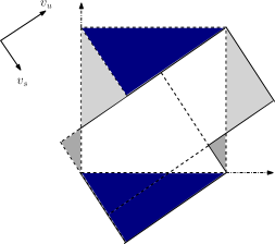
Figure 2.1. The construction of the Markov partition

The adjacency Matrix of the Markov partition is then defined by $A_{i,j}=1$ if and only if ${\rm int}R_{i}\cap f^{-1}\left({\rm int}R_{j}\right)\neq\emptyset$. Here the adjacency Matrix is

$${\bf A}=\left(\begin{array}[]{ccc}1&0&1\\ 1&0&1\\ 0&1&0\end{array}\right).$$

Let $\Phi:\Sigma_{A}\to\mathbb{T}^{2}$ be the map defined by $\Phi(x):=\bigcap_{n=-\infty}^{\infty}\overline{f^{-n}R_{x_{n}}}$. Note that by the Baire Category Theorem since $\left\{\cap_{n=-N}^{N}\overline{f^{-n}R_{x_{n}}}\right\}_{N=1}^{\infty}$ is a decreasing sequence of compact sets, $\Phi(x)$ is well defined. The map $\Phi:\Sigma_{{\bf A}}\to\mathbb{T}^{2}$ is continuous, finite to one, and for every $x\in\Sigma_{{\bf A}}$,

$$\Phi\circ T(x)=f\circ\Phi(x).$$

In other words, $\Phi$ is a semi-conjugacy (topological factor map) between $\left(\Sigma_{{\bf A}},T\right)$ to $\left(\mathbb{T}^{2},f\right)$. In addition, for every $x\in\mathbb{T}^{2}\backslash\cup_{n\in\mathbb{Z}}\cup_{i=1}^{3}f^{-n}\left(\partial R_{i}\right)$ there exists a unique $w\in\Sigma_{{\bf A}}$ so that $\Phi(w)=x$ . The Lebesgue measure $m_{\mathbb{T}^{2}}$ on $\mathbb{T}^{2}$ is invariant under $f$. One can check that $m_{\mathbb{T}^{2}}\left(\cup_{i=1}^{3}\partial R_{i}\right)=0$ and thus $\Phi^{-1}$ defines an isomorphism between $\left(\mathbb{T}^{2},m_{\mathbb{T}^{2}},f\right)$ and $\left(\Sigma_{{\bf A}},\mu_{\pi_{{\bf Q}},{\bf Q}},T\right)$ where $\mu_{\pi_{{\bf Q}},{\bf Q}}$ is the stationary Markov measure with

(2.1) $$P_{j}\equiv\mathbf{Q}:=\left(\begin{array}[]{ccc}\frac{\varphi}{1+\varphi}&0&\frac{1}{1+\varphi}\\ \frac{\varphi}{1+\varphi}&0&\frac{1}{1+\varphi}\\ 0&1&0\end{array}\right)$$

and

(2.2) $$\pi_{j}=\mathbf{{\bf\pi_{Q}}}:=\left(1/\sqrt{5},\ 1/\varphi\sqrt{5},\ 1/\varphi\sqrt{5}\right)=\left(m_{\mathbb{T}^{2}}\left(R_{1}\right),m_{\mathbb{T}^{2}}\left(R_{2}\right),m_{\mathbb{T}^{2}}\left(R_{3}\right)\right).$$

2.2.1. Nonsingular Markov shifts:

Let $\left\{P_{n}\right\}_{n=-\infty}^{\infty}\subset M_{S\times S}$ be a sequence of aperiodic and irreducible stochastic matrices on $S.$ In addition let $\left\{\pi_{n}\right\}_{n=-\infty}^{\infty}$ be a sequence of probability distributions on $S$ so that for every $s\in S$ and $n\in\mathbb{Z}$,

(2.3) $$\sum_{t\in S}\pi_{n-1}(t)\cdot P_{n}\left(t,s\right)=\pi_{n}(s).$$

Then one can define a measure on the collection of cylinder sets,

$$[b]_{k}^{l}:=\left\{x\in S^{\mathbb{Z}}:\ x_{j}=b_{j}\ \forall j\in[k,l]\cap\mathbb{Z}\right\}$$

by

$$\mu\left(\left[b\right]_{k}^{l}\right):=\pi_{k}\left(b_{k}\right)\prod_{j=k}^{l-1}P_{j}\left(b_{j},b_{j+1}\right).$$

Since the equation (2.3) is satisfied, $\mu$ satisfies the consistency condition and therefore by Kolmogorov’s extension theorem $\mu$ defines a measure on $S^{\mathbb{Z}}$. In this case we say that $\mu$ is the Markov measure generated by $\left\{\pi_{n},P_{n}\right\}_{n\in\mathbb{Z}}$ and denote $\mu=\text{M}\left\{\pi_{n},P_{n}:\ n\in\mathbb{Z}\right\}$. By $\text{M}\left\{\pi,P\right\}$ we mean the measure generated by $P_{n}\equiv P$ and $\pi_{n}\equiv\pi$. We say that $\mu$ is nonsingular for the shift $T$ on $S^{\mathbb{Z}}$ if $T_{*}\mu\sim\mu$.

2.3. Local absolute continuity

Let $(X,\mathcal{B})$ be a measure space and $\mathcal{F}_{n}\subset\mathcal{B}$ be a filtration of $X$. That is an increasing sequence of $\sigma$-algebras such that $\mathcal{F}_{n}\uparrow\mathcal{B}$. The method in [KBL, Shi] uses ideas from Martingale theory in order to determine whether two Borel probability measures $\mu,\nu$ are absolutely continuous.

Definition 3.

Given a filtration $\left\{\mathcal{F}_{n}\right\}$, we say that $\nu\ll^{loc}\mu$ ($\nu$ is locally absolutely continuous with respect to $\mu$) if for every $n\in\mathbb{N}$, $\nu_{n}\ll\mu_{n}$ where $\nu_{n}=\nu|_{\mathcal{F}_{n}}.$

Suppose that $\nu\ll^{loc}\mu$ w.r.t $\left\{\mathcal{F}_{n}\right\}$, set $z_{n}:=\frac{d\nu_{n}}{d\mu_{n}}$. The sequence $z_{n}$ is a nonnegative martingale with respect to $\mathcal{F}_{n}$ and thus by the martingale convergence theorem there exists a $[0,\infty]$ valued random variable $z_{\infty}$ such that $\lim_{n\to\infty}z_{n}=z_{\infty}$ a.s. It follows that if $\nu\ll^{loc}\mu$ then $\nu\ll\mu$ if and only if $z_{n}\xrightarrow[n\to\infty]{}z_{\infty}$ in $L^{1}\left(\mu\right)$. The latter holds if and only if the sequence $\left\{z_{n}\right\}_{n=1}^{\infty}$ is uniformly integrable meaning that for all $\epsilon>0$ there exists $M>0$ such that for all $n\in\mathbb{N}$, $\int z_{n}1_{\left[z_{n}>M\right]}d\mu<\epsilon$.

2.4. Sections Overview and explanation of the method of construction

The idea is as follows, let $f(x,y)=(x+y,x){\rm mod}1$, $\left\{R_{1},R_{2},R_{3}\right\}$ be the corresponding Markov partition for $f$, $\Sigma_{A}$ the resulting topological Markov shift and $\Phi:\ \Sigma_{{\bf A}}\to\mathbb{T}^{2}$ the topological semiconjugacy with the shift. In addition $\mathbf{Q}$ will always denote the transition matrix corresponding to the Lebesgue measure.

• In Section 3 we present an inductive construction which produces a family of nonatomic inhomogeneous Markov measures which are fully supported on $\Sigma_{A}\subset\{1,2,3\}^{\mathbb{Z}}$ and are of type ${\rm III}_{1}$.

• Let $\mu$ be such a Markov measure generated by $\left\{\pi_{k},P_{k}:\ k\in\mathbb{Z}\right\}$. Since $\mu$ is conservative $\Phi_{*}\mu$ gives zero measure to the images of the boundaries of the rectangles of the Markov partition. The latter property implies that $\Phi$ is an isomorphism of $\left(\mathbb{T}^{2},\Phi_{*}\mu,f\right)$ and $\left(\Sigma_{{\bf A}},\mu,Shift\right)$ and thus $\left(\mathbb{T}^{2},\Phi_{*}\mu,f\right)$ is a type ${\rm III}_{1}$ dynamical system.

The type ${\rm III}_{1}$, inhomogeneous Markov measures for the shift on $\Sigma_{{\bf A}}$ have the additional property that for every $k\leq 0$ the transition matrices of $\mu$ at $k$ are the same as the ones arising from the Lebesgue measure ($\forall k\leq 0,\ P_{k}={\bf Q}$). This implies that (after a rotation of the coordinates to the $v_{u},v_{s}$ coordinates) with $\Phi:\Sigma_{{\bf A}}\to\mathbb{T}$ being the semiconjugacy map arising from the Markov partition we have

$$d\Phi_{*}\mu(x,y)=d\nu^{+}(x)dy.$$

Here $\nu^{+}$ is the image by the push forward on the stable manifold of the Markov measure on $\{1,2,3\}^{\mathbb{N}}$ given by $\left\{\pi_{k},P_{k}\right\}_{k=1}^{\infty}$. This property will be used (see Subsection 2.5) to show that there exists an homeomorphism $G$ of $\mathbb{T}^{2}$ such that $m_{\mathbb{T}^{2}}\circ G=\Phi_{*}\mu$ and the transformation $G\circ f\circ G^{-1}:\left(\mathbb{T}^{2},m_{\mathbb{T}^{2}}\right)\to\left(\mathbb{T}^{2},m_{\mathbb{T}^{2}}\right)$ is measure theoretically isomorphic to $\left(\mathbb{T}^{2},\Phi_{*}\mu,f\right)$, hence a type ${\rm III}_{1}$ system.

The harder part in the proof of this theorem is to construct a homeomorphism $H:\mathbb{T}^{2}\to\mathbb{T}^{2}$ so that

1. $m\circ H\sim\Phi_{*}\mu=m\circ G$. Consequently the system $\left(\mathbb{T}^{2},\mathcal{B}_{\mathbb{T}^{2}},m_{\mathbb{T}^{2}},H\circ f\circ H^{-1}\right)$ is of type ${\rm III}_{1}$ because it is measure theoretically isomorphic to $\left(\mathbb{T}^{2},\mathcal{B}_{\mathbb{T}^{2}},m_{\mathbb{T}^{2}}\circ H,f\right)$ and the fact that the type ${\rm III}_{1}$ property is invariant upon changing the measure to an equivalent measure.

2. $H\circ f\circ H{}^{-1}$ is $C^{1}$ and Anosov.

In order to obtain this goal and to explain the definition of $G$ it is easier for us to build $f$ as the natural extension of (the non invertible) golden mean shift $Sx=\varphi x{\rm mod}1$.

2.5. The map $f$ as the natural extension of the golden mean shift

The partition $\left\{J_{1}=[0,1/\varphi^{2}],\ J_{2}=[1/\varphi,1],\ J_{3}=\left[1/\varphi^{2},1/\varphi\right]\right\}$ is a Markov partition for the golden mean shift with ${\bf A}$ (the same matrix as the one for $f$) as its adjacency matrix. See figure 2.2.

Figure 2.2. The Markov partition of $\varphi x\mod 1$

Denote by $\sigma$ the one sided shift on $\Sigma_{{\bf A}}^{+}$. It can be verified that $\left(\Sigma_{{\bf A}}^{+},\nu_{\pi_{{\bf Q}},{\bf Q}},\sigma\right)$ is isomorphic to $\left(\mathbb{T},m_{{\rm\mathbb{T}}},S\right)$ where $m_{\mathbb{T}}$ is the Lebesgue measure on $\mathbb{T}$. The natural extension of $\left(\Sigma_{{\bf A}}^{+},\nu_{\pi_{{\bf Q}},{\bf Q}},\sigma\right)$ is $\left(\Sigma_{{\bf A}},\text{M}\left\{\pi_{{\bf Q}},{\bf Q}\right\},\sigma\right)$ which is isomorphic to $\left(\mathbb{T}^{2},m_{{\rm Leb}},f\right)$. This shows that $f$ is indeed the natural extension of the Golden mean shift. To see the geometric picture of how $S$ and $f$ are related one can look at the Markov partitions and move to the $V_{u},V_{s}$ coordinates. On those coordinates $f$ acts almost as

$$(u,v)\mapsto\left(\varphi u\mod 1,-\varphi^{-1}v\right)=\left(Su,-\varphi^{-1}v\right),$$

where the mistake is in the second coordinate. To make it precise let $\mathbb{M}=\left[0,1/\varphi\right]\times\left[-\varphi/\left(\varphi+2\right),\varphi^{2}/\left(\varphi+2\right)\right]\bigcup\left[1/\varphi,1\right]\times\left[-\varphi/\left(\varphi+2\right),1/\left(\varphi+2\right)\right]$. Define $\tilde{f:}\mathbb{M}\to\mathbb{M}$ by

$$\tilde{f}(x,y)=\begin{cases}\left(\varphi x,-\varphi^{-1}y\right),&0\leq x\leq 1/\varphi\\ \left(\varphi x-1,-\varphi^{-1}\left(y-\frac{\varphi^{2}}{\varphi+2}\right)\right),&1/\varphi\leq x\leq 1\end{cases}.$$

See Figure 2.3 for the way $\tilde{f}$ maps its 3 rectangles, as can be seen by this picture the action of $\tilde{f}$ is the same as how $f$ acts on its Markov partition.

Figure 2.3. Action of $\tilde{f}$ on it’s (soon to be) Markov partition

In order that $\tilde{f}$ will be the same as $f$, we identify by orientation preserving piecewise translations the following intervals (for a geometric understanding one can see that this identification comes from the way the Markov partition of $f$ tiles the plane):

$$\{0\}\times\left[0,\varphi^{2}/\left(\varphi+2\right)\right] \simeq \{1\}\times\left[-\varphi/\left(\varphi+2\right),1/\left(\varphi+2\right)\right]$$

$$\{0\}\times\left[-\varphi/\left(\varphi+2\right),0\right] \simeq \left\{1/\varphi\right\}\times\left[1/\left(\varphi+2\right),\varphi^{2}/\left(\varphi+2\right)\right]$$

$$\left[0,1/\varphi^{3}\right]\times\left\{\varphi^{2}/\left(\varphi+2\right)\right\} \simeq \left[1/\varphi^{2},1/\varphi\right]\times\left\{-\varphi/\left(\varphi+2\right)\right\}$$

$$\left[1/\varphi^{3},1/\varphi\right]\times\left\{\varphi^{2}/\left(\varphi+2\right)\right\} \simeq \left[1/\varphi,1\right]\times\left\{-\varphi/\left(\varphi+2\right)\right\}$$

$$\left[0,1/\varphi^{2}\right]\times\left\{-\varphi/\left(\varphi+2\right)\right\} \simeq \left[1/\varphi,1\right]\times\left\{1/\left(\varphi+2\right)\right\}.$$

The resulting Manifold (which is $\mathbb{T}^{2}$) will be denoted by $\mathbb{M}_{\sim}$ in order to remind the reader of this change of coordinates and the geometric relation between $f$ and $S$.

In $\mathbb{M}_{\sim}$, $d\Phi_{*}\mu(x,y)=d\nu^{+}(x)dy$ where $\nu^{+}$ is a non atomic measure on $\mathbb{T}$. This means that the circle homeomorphism $h(x)=\nu^{+}[0,x]$ takes the Lebesgue measure on $\mathbb{T}$ to $\nu^{+}$ and $h\left(1/\varphi\right)=\mu\left(x_{1}\neq 2\right)=\frac{1}{\varphi}$. The homeomorphism of $\mathbb{M}_{\sim}$ defined by $G(x,y)=(h(x),y)$ takes Lebesgue measure of $\mathbb{M}_{\sim}$ to $\Phi_{*}\mu$. The perturbed homeomorphism $H:\mathbb{M}_{\sim}\to\mathbb{M}_{\sim}$ which will be constructed is of the form $H(x,y)=\left(h_{y}(x),y\right)$, where for $y\in\left[-\varphi/\left(\varphi+2\right),\varphi^{2}/\left(\varphi+2\right)\right]$, $h_{y}:\mathbb{T}\to\mathbb{T}$ is a circle homeomorphism such that $m_{\mathbb{T}}\circ h_{y}\sim\nu^{+}$. This construction is carried out by the following steps:

• the first step is to work on the action of $f$ on the unstable manifold which is the Golden mean shift and to construct a circle homeomorphism $\tilde{h}$ such that $\tilde{h}\circ S\circ\tilde{h}^{-1}$ is $C^{1}$ expanding and $m_{\mathbb{T}}\circ\tilde{h}\sim\nu^{+}$. A further important property of the homeomorphisms which we construct is that $\tilde{h}\left(J_{i}\right)=J_{i}$ for all elements of the Markov partition of $S$. This will imply for example that $\left(\tilde{h}(x),y\right)$ is an homeomorphism of $\mathbb{M}_{\sim}$. This step involves adding another parameter for the inductive construction of the measure $\mu=\text{M}\left\{P_{k},\pi_{k}:\ k\in\mathbb{Z}\right\}$ and is carried out in Section 4.

• in Section 5 we modify construction of these homeomorphisms $\tilde{h}$ in order to construct the functions $h_{y}$ in the definition of $H$. A major challenge in this step is to ensure that $\frac{\partial H\circ\tilde{f}\circ H^{-1}}{\partial y}$ is defined and continuous.

3. The type ${\rm{\rm III}_{1}}$ Markov shifts supported on $\Sigma_{A}$

Here we present the inductive construction of the inhomogeneous Markov measures.

3.1. Markov Chains

3.1.1. Basics of Stationary (homogenous) Chains

Let $S$ be a finite set which we regard as the state space of the chain, $\pi=\left\{\pi(s)\right\}_{s\in S}$ a probability vector on $S$ and ${\rm P}=\left(P_{s,t}\right)_{s,t\in S}$ a stochastic matrix. The vector $\pi$ and ${\rm P}$ define a Markov chain $\left\{X_{n}\right\}$ on $S$ by

$$\forall n\in\mathbb{Z},\ \ \mathbb{P}_{\pi}\left(X_{n}=t\right)\pi(t)\ \ \text{\ and\ \ }\ \mathbb{P}\left(X_{n}=s\left|X_{1},..,X_{n-1}\right.\right):=P_{X_{n-1},s}.$$

${\rm P}$ is irreducible if for every $s,t\in S$, there exists $n\in\mathbb{N}$ such that $P_{s,t}^{n}>0$ and ${\rm P}$ is aperiodic if for every $s\in S$, ${\rm gcd}\left\{n:\ P_{s,s}^{n}>0\right\}=1$. Given an irreducible and aperiodic ${\rm P}$, there exists a unique stationary probability $\pi_{{\rm P}}$ (that is $\pi_{P}{\rm P}=\pi_{P}$). In addition for every $s,t\in S$, $P_{s,t}^{n}\xrightarrow[n\to\infty]{}\pi_{P}(t)$. Since $S$ is a finite state space, it follows that for any initial distribution $\pi$ on $S$,

$$\mathbb{P}_{\pi}\left(X_{n}=t\right)=\sum_{s\in S}\pi(s)P_{s,t}^{n}\xrightarrow[n\to\infty]{}\pi_{P}(t).$$

An important fact which will be used in the sequel is that the stationary distribution is continuous with respect to the stochastic matrix. That is if $\left\{{\rm P_{n}}\right\}_{n=1}^{\infty}$ is a sequence of irreducible and aperiodic stochastic matrices such that

$$\|{\rm P}_{n}-{\rm P\|_{\infty}:=}\max_{s,t\in S}\left|\left({\rm P}_{n}\right)_{s,t}-{\rm P}_{s,t}\right|\xrightarrow[n\to\infty]{}0$$

and ${\rm P}$ is irreducible and aperiodic then $\left\|\pi_{{\rm P}_{n}}-\pi_{{\rm P}}\right\|_{\infty}\to 0$.

3.2. Type ${\rm III_{1}}$ Markov Shifts

In this subsection, let $\Omega:=\Sigma_{{\bf A}}$, $\mathcal{B}:=\mathcal{B}_{\Sigma_{{\bf A}}}$ and $T$ is the two sided shift on $\Omega$. For two integers $k<l$, write $\mathcal{F}\left(k,l\right)$ for the algebra of sets generated by cylinders of the form $[b]_{k}^{l},\ b\in\{1,2,3\}^{l-k}$. That is the smallest $\sigma$-algebra which makes the coordinate mappings $\left\{w_{i}(x):=x_{i}:i\in[k,l]\right\}$ measurable.

3.2.1. Idea of the construction of the type ${\rm III}$ Markov measure.

The construction uses the ideas in [Kos]. For every $j\leq 0$

$$P_{j}\equiv\mathbf{Q}\ {\rm and}\ \pi_{j}\equiv\pi_{\mathbf{Q}},$$

where $\mathbf{Q}$ and $\pi_{\mathbf{Q}}$ are as in (2.1) and (2.2) respectively. On the positive axis one defines on larger and larger chunks the stochastic matrices which depend on a distortion parameter $\lambda_{k}\geq 1$ where $1$ means no distortion. Now a cylinder set $[b]_{-n}^{n}$ fixes the values of the first $n$ terms in the product form of the Radon Nykodym derivatives. We would like to be able to correct the values in order that we can enforce a given number to be in the ratio set. This corresponds to a lattice condition on $\lambda_{k}$ which is less straightforward then the one in [Kos]. However this is not enough for a Markov measure, since the states are not independent, this forces us to utilize both the convergence to the stationary distribution and the mixing property for stationary chains.

Another difficulty is that the measure of the set $[b]_{-n}^{n}\cap T^{-N}[b]_{-n}^{n}\cap\left\{\left(T^{N}\right)^{\prime}\approx a\right\}$ could be of very small measure with respect to $\mu\left([b]_{-n}^{n}\right)$. To remedy this problem, and enable approximation of general sets, we look for many approximately independent such events so that their union covers at least a fixed proportion of $[b]_{-n}^{n}$.

More specifically the construction goes as follows. We define inductively $5$ sequences $\left\{\lambda_{j}\right\}$, $\left\{m_{j}\right\}$, $\left\{n_{j}\right\}$, $\left\{N_{j}\right\}$ and $\left\{M_{j}\right\}$ where

$$M_{0} = 1$$

$$N_{j} := N_{j-1}+n_{j}$$

$$M_{j} := N_{j}+m_{j}.$$

This defines a partition of $\mathbb{N}$ into segments $\left\{\left[M_{j-1},N_{j}\right),\ \left[N_{j},M_{j}\right)\right\}_{j=1}^{\infty}$. The sequence $\left\{P_{n}\right\}$ equals $\mathbf{Q}$ on the $\left[N_{j},M_{j}\right)$ segments while on the $\left[M_{j-1},N_{j}\right)$ segments we have $P_{n}\equiv\mathbf{Q}_{\lambda_{j}}$, the $\lambda_{j}$ perturbed stochastic matrix. The $\mathbf{Q}$ segments facilitate the form of some of the Radon Nykodym derivatives while the perturbed segments come to ensure that $\mu\perp\text{M}\left\{\pi_{{\bf Q}},{\bf Q}\right\}$ and that the ratio set condition is satisfied for cylinder sets.

Notation: By $x=a\pm b$ we mean $a-b\leq x\leq a+b$.

3.2.2. The construction.

For $\lambda\geq 1$ let

$$\mathbf{Q_{\lambda}}:=\left(\begin{array}[]{ccc}\frac{\varphi\lambda}{1+\varphi\lambda}&0&\frac{1}{1+\varphi\lambda}\\ \frac{\varphi}{1+\varphi}&0&\frac{1}{1+\varphi}\\ 0&1&0\end{array}\right).$$

Choice of the base of induction: Let $M_{0}=1,\ \lambda_{1}>1$, $n_{1}=2$, $N_{1}=3$ and ${\bf Q}_{1}:={\bf Q}_{\lambda_{1}}$ be the $\lambda_{1}$ perturbed matrix. Set $P_{1}=P_{2}=\mathbf{Q}_{\mathbf{1}}$ and $\pi_{0}=\pi_{\mathbf{Q}}$. The measures $\pi_{1},\pi_{2}$ are then defined by equation (2.3). Let $m_{1}=3$ and thus $M_{1}=6.$ Set $P_{j}=\mathbf{Q}$ for $j\in\left[N_{1},M_{1}\right)=\left[3,6\right)$ and $\pi_{3},\pi_{4},\pi_{5}$ be defined by equation (2.3).

Assume that $\left\{\lambda_{j},m_{j},n_{j},N_{j},M_{j}\right\}_{j=1}^{l-1}$ have been chosen.

Choice of $\lambda_{l}$: Notice that the function $f(x):=x\frac{1+\varphi}{1+\varphi x}$ is monotone increasing and continuous in the segment $[1,\infty)$. Therefore we can choose $\lambda_{l}>1$ which satisfies the following three conditions:

1. Finite approximation of the Radon-Nykodym derivatives condition:

   (3.1) $$\left(\lambda_{l}\right)^{2m_{l-1}}<e^{\frac{1}{2^{l}}}.$$

   This condition ensures an approximation of the derivatives by a finite product.

2. Lattice condition:

   (3.2) $$\lambda_{l-1}\cdot\frac{1+\varphi}{1+\varphi\lambda_{l-1}}\in\left(\lambda_{l}\cdot\frac{1+\varphi}{1+\varphi\lambda_{l}}\right)^{\mathbb{N}},$$

   where $a^{\mathbb{N}}:=\left\{a^{n}:n\in\mathbb{N}\right\}$.

3. Let ${\bf Q}_{l}:={\bf Q}_{\lambda_{l}}$ and $\pi_{\mathbf{Q_{l}}}$ be its unique stationary probability. Notice that when $\lambda_{l}$ is close to $1$, then $\mathbf{Q_{l}}$ is close to $\mathbf{Q}$ in the $L_{\infty}$ sense. Therefore by continuity of the stationary distribution we can demand that

   (3.3) $$\|\pi_{\mathbf{Q}}-\pi_{\mathbf{Q_{l}}}\|_{\infty}<\frac{1}{2^{l}}.$$

Choice of $n_{l}$: It follows from the Lattice condition, equation (3.2), that for each $k\leq l-1$,

$$\left(\lambda_{k}\cdot\frac{1+\varphi}{1+\varphi\lambda_{k}}\right)\in\left(\lambda_{l}\cdot\frac{1+\varphi}{1+\varphi\lambda_{l}}\right)^{\mathbb{N}}.$$

Choose $n_{l}$ large enough so that for every $k\leq l-1$ (notice that the demand on $k=1$ is enough) there exists $\mathbb{N}\ni p=p(k,l)\leq\frac{n_{l}}{20}$ so that

(3.4) $$\left(\lambda_{l}\cdot\frac{1+\varphi}{1+\varphi\lambda_{l}}\right)^{p}=\left(\lambda_{k}\cdot\frac{1+\varphi}{1+\varphi\lambda_{k}}\right).$$

Till now we have defined $\left\{P_{j},\pi_{j}\right\}_{j=-\infty}^{M_{l-1}}$. By the mean ergodic theorem for Markov chains [LPW, Th. 4.16] and (3.3), one can demand by enlarging $n_{l}$ if necessary that in addition

(3.5) $$\nu_{\pi_{M_{l-1}},\mathbf{Q_{l}}}\left(x:\ \frac{1}{n_{l}}\sum_{j=1}^{n_{l}}{\bf 1}_{\left[x_{j}=1\right]}=\frac{1}{\sqrt{5}}\pm 2^{-l}\right)>1-\frac{1}{l},$$

and

(3.6) $$\nu_{\pi_{M_{l-1}},\mathbf{Q_{l}}}\left(x:\ \frac{1}{n_{l}}\sum_{j=1}^{n_{l}}{\bf 1}_{\left[x_{j}=2,x_{j+1}=3\right]}>\frac{1}{15}\right)>1-\frac{1}{l},$$

where $\nu$ is the Markov measure on $\{1,2,3\}^{\mathbb{N}}$ defined by and ${\rm\mathbf{Q_{l}}}$ and $\pi_{M_{t-1}}$. The numbers inside the set were chosen so that

$$\left|\pi_{\mathbf{Q_{l}}}(1)-1/\sqrt{5}\right|<2^{-l},$$

and similarly for $l$ large enough

$$\int{\bf 1}_{\left[x_{0}=2,x_{1}=3\right]}(x)d\nu_{\pi_{\mathbf{Q_{l}}},\mathbf{Q_{l}}} = \pi_{\mathbf{Q_{l}}}(2)\left(\mathbf{Q_{l}}\right)_{2,3}=\left(\frac{1}{\varphi\sqrt{5}}\pm\frac{1}{2^{l}}\right)\frac{1}{\varphi+1}>\frac{1}{15}.$$

Choice of $N_{l}$: Let $N_{l}:=M_{l-1}+n_{l}$. Now set for all $j\in\left[M_{l-1},N_{l}\right)$,

$$P_{j}=\mathbf{Q_{l}}$$

and $\left\{\pi_{j}\right\}_{j=M_{l-1}+1}^{N_{l}}$ be defined by equation (2.3).
Choice of $m_{l}$: Let $k_{l}$ be the $\left(1\pm\left(\frac{1}{3}\right)^{3N_{l}}\right)$ mixing time of $\mathbf{Q}$. That is for every ${\bf n}>k_{l}$, $j\in\mathbb{N}$, $A\in\mathcal{F}\left(0,j\right)$, $B\in\mathcal{F}\left(j+{\bf n},\infty\right)$ and initial distribution $\tilde{\pi}$,

(3.7) $$\nu_{\tilde{\pi},\mathbf{Q}}\left(A\cap B\right)=\left(1\pm 3^{-3N_{l}}\right)\nu_{\tilde{\pi},\mathbf{Q}}\left(A\right)\nu_{\pi_{\mathbf{Q}},\mathbf{Q}}\left(T^{{\bf n}+l}B\right).$$

Demand in addition that $k_{l}>N_{l}$. Let $m_{l}$ be large enough so that

(3.8) $$\left(1-9^{-3N_{l}}\right)^{m_{l}/4k_{l}}\leq\frac{1}{l},$$

and

(3.9) $$\left(m_{l}-N_{l}\right)\lambda_{1}^{-2N_{l}}\geq 1.$$

To summarize the construction. We have defined inductively sequences $\left\{n_{l}\right\},\ \left\{N_{l}\right\},\ \left\{m_{l}\right\},\ \left\{M_{l}\right\}$ of integers which satisfy

$$M_{l}<N_{l+1}=M_{l}+n_{l}<M_{l+1}=N_{l+1}+m_{l+1}.$$

In addition we have defined a monotone decreasing sequence $\left\{\lambda_{l}\right\}$ which decreases to $1$ and using that sequence we defined new stochastic matrices $\left\{\mathbf{Q_{l}}\right\}$. Now we set

(3.10) $$P_{j}:=\begin{cases}\mathbf{Q},&j\leq 0\\ \mathbf{Q_{l}},&M_{l-1}\leq j<N_{l}\\ \mathbf{Q},&N_{l}\leq j<M_{l}\end{cases},$$

and $\pi_{j}=\pi_{{\rm P}}$ for $j\leq 0$. The rest of the $\pi_{j}$’s are defined by the consistency condition, equation (2.3). Finally let $\mu$ be the Markovian measure on $\left\{1,2,3\right\}^{\mathbb{Z}}$ defined by $\left\{\pi_{j},P_{j}\right\}_{j=-\infty}^{\infty}$.

Notice that for all $j\in\mathbb{N}$, ${\rm supp}P_{j}\equiv{\rm supp}A={\rm supp}\mathbf{Q}$.

Theorem 4.

The shift $\left(\left\{1,2,3\right\}^{\mathbb{Z}},\mu,T\right)$ is nonsingular,conservative, ergodic and of type ${\rm III}_{1}$.

The proof of Theorem 4 is given in the appendix.

4. Type ${\rm III}$ perturbation of the Golden Mean Shift arising from Markovian measures

4.1. A perturbation of the golden mean shift:

Let $\nu=\text{M}\left\{\pi_{k},{\rm P}_{k}\right\}_{k=-\infty}^{\infty}$ be the type ${\rm III_{1}}$ (for the shift on $\left\{1,2,3\right\}^{\mathbb{Z}}$) Markov measure from Section 3 for the two sided shift. It follows from [ST, Thm. 4.4.] that the one sided Markov measure $\nu^{+}=\text{M}\left\{\pi_{k},{\rm P}_{k}\right\}_{k=1}^{\infty}$ on $\left\{1,2,3\right\}^{\mathbb{N}}$ is a type ${\rm III}$ measure for the (one sided) shift.

Let $Sx=\varphi x\mod 1$ and $J_{1}:=\left(0,1/\varphi^{2}\right)$, $J_{2}:=\left(1/\varphi,1\right)$ and $J_{3}:=\left(1/\varphi^{2},1/\varphi\right)$ be a Markov partition for $S$. Denote by

$${\rm Bd}\left(S\right):=\bigcup_{n=0}^{\infty}\bigcup_{i=1}^{3}\partial\left(S^{-n}J_{i}\right).$$

The map $\Theta:\Sigma_{{\bf A}}^{+}\to[0,1]$, $\Theta\left(w\right)=\bigcap_{n=0}^{\infty}\overline{S^{-n}J_{w_{n}}}$ is a semiconjugacy of $\left(\Sigma_{{\bf A}}^{+},\sigma\right)$ and $\left(\mathbb{T},S\right)$ and for each $x\notin{\rm Bd}\left(S\right)$, $\Theta^{-1}(x)$ consists of one point (point of uniqueness for the $\Theta$ representation). Since the support of $\nu^{+}$ is contained in ${\rm G}\left(\sigma\right):=\Theta^{-1}\left(\mathbb{T}\backslash{\rm Bd}\left(S\right)\right)$, the map ${\rm\Theta}$ is a metric isomorphism between $\left(\Sigma_{{\bf A}}^{+},\nu^{+},\sigma\right)$ and $\left(\mathbb{T},\Theta_{*}\left(\nu^{+}\right),S\right)$ and therefore the measure $\mu^{+}:=\Theta_{*}\left(\nu^{+}\right)$ is a type ${\rm III}$ measure for $S$. Since $\mu^{+}$ is a continuous measure, its cumulative distribution function $\mathfrak{h}(x)=\mu^{+}\left(\left[0,x\right]\right)$ is a homeomorphism of $\mathbb{T}$ such that $\mu^{+}\circ\mathfrak{h}^{-1}$ is Lebesgue measure on $\mathbb{T}$. It follows that the map $\left(\mathbb{T},m_{\mathbb{T}},\mathfrak{h}\circ S\circ\mathfrak{h}^{-1}\right)$ is a type ${\rm III}$ transformation, where $m_{\text{$\mathbb{T}$}}$ denotes the Lebesgue measure. The problem is that $\mathfrak{h}\circ S\circ\mathfrak{h}^{-1}$ is not necessarily smooth, so we construct $\mathfrak{h}_{\epsilon}$, as in the idea of the examples of Bruin and Hawkins, close to $\mathfrak{h}$ in the $C^{0}$ norm such that

• $\mathfrak{h}_{\epsilon}\circ S\circ\mathfrak{h}_{\epsilon}^{-1}$ is $C^{1}$ and uniformly expanding.

• $m_{\text{$\mathbb{T}$}}\circ\mathfrak{h}_{\epsilon}\sim\mu^{+}$.

• We will have in addition that $\mathfrak{h}_{\mathbb{\epsilon}}J_{i}=J_{i}$ for every $i\in\{1,2,3\}$, this extra property is crucial for the extension to two dimensions.

Before we go through the construction we would like the reader to recall that the Lebesgue measure on $\mathbb{T}$ is the measure arising from $\text{M}\left\{\pi,{\bf Q}\right\}$. The main idea is to approximate the change of measure between Lebesgue measure and $\mu^{+}$ on the semi algebras

$$\mathcal{R}(n):=\left\{C_{\left[w\right]_{1}^{n}}:=\bigcap_{k=0}^{n-1}S^{-k}J_{w_{k}}:x\in\Sigma_{{\bf A}}\right\}=\left\{C_{w}:\ w\in\Sigma_{{\bf A}}(n)\right\}.$$

The construction goes as follows: We first assume that we are given a type ${\rm III}$ Markovian measure defined by $\left\{\lambda_{k},M_{k},N_{k}\right\}_{k=1}^{\infty}$. Then we would like to choose inductively, mostly by continuity arguments a sequence $\underline{\epsilon}=\left\{\epsilon_{k}\right\}$ that will give us the perturbation. However in the end we arrive at a problem that we need that the size of $M_{k}$ is relatively large with respect to $1/\epsilon_{k-1}$. This problem will be solved by modifying the induction process of Section 3 and adding the choice of the sequence $\underline{\epsilon}$ to the induction. The new induction will be explained in Subsection 4.2.2.

Remark 5.

Before we continue with the construction we would like to remind the reader that at each stage in the inductive construction of the Markovian measure in Section 3 we can take $\lambda_{t}$ to be as close to $1$ as we like and $n_{t},\ M_{t}/N_{t}$ to be as large as we want. This is because the conditions on $\lambda_{t}$ ((3.1), (3.2) and (3.3)) are that $\lambda_{t}$ is small enough whilst the conditions on $n_{t}$ ((3.4), (3.5) and (3.6)) and $M_{t}/n_{t}\sim m_{t}/n_{t}$ ((3.8) and (3.9)) are to be large enough.

Special interpolation functions:

Given $\alpha>0$ we would like to define a Lipschitz function $g_{\alpha}$ so that $g_{\alpha}(0)=0$, $g^{\prime}_{\alpha}(0)=1$, $g_{\alpha}(1)=\int_{0}^{1}g_{\alpha}^{\prime}(x)dx=\alpha$ and $g_{\alpha}^{\prime}(1)=\alpha$. We will use the functions $g_{\alpha}:[0,1]\to[0,\alpha]$ defined by $g_{\alpha}(0)=0$ and

$$g^{\prime}_{\alpha}(x)=\begin{cases}1+3x\cdot\frac{5\alpha-5}{4}&0\leq x\leq\frac{1}{3}\\ \frac{5\alpha-1}{4},&\frac{1}{3}\leq x\leq\frac{2}{3}\\ \frac{5\alpha-1}{4}-(3x-2)\frac{\alpha-1}{4},&\frac{2}{3}\leq x\leq 1\end{cases}$$

which have the additional property that if $\alpha>1$ then

$$1=\inf_{x\in[0,1]}g^{\prime}_{\alpha}(x)<\sup_{x\in[0,1]}g^{\prime}_{\alpha}(x)=\frac{5\alpha-1}{4}<\alpha^{2}$$

and if $\frac{1}{4}\leq\alpha<1$ then

$$\alpha^{2}\leq\frac{5\alpha-1}{4}=\inf_{x\in[0,1]}g^{\prime}_{\alpha}(x)<\sup_{x\in[0,1]}g^{\prime}_{\alpha}(x)=1.$$

Remark 6.

For all $\alpha,\epsilon>0$,

$$\int_{0}^{\epsilon}g_{\alpha}^{{}^{\prime}}\left(\frac{x}{\epsilon}\right)dx=\epsilon\int_{0}^{1}g^{\prime}_{\alpha}(x)dx=\epsilon\alpha$$

and for all $u>\epsilon$,

$$\int_{u-\epsilon}^{u}g_{\alpha}^{{}^{\prime}}\left(\frac{u-x}{\epsilon}\right)dx=\epsilon\alpha$$

4.2. Realization of the homeomorphism of change of measures

For $0<\epsilon<\frac{1}{\varphi}$ and $\lambda>1$, let $\psi_{\epsilon,\lambda}:\left[0,1\right]\circlearrowleft$ be the function defined by $\psi_{\epsilon,\lambda}(0)=0$ and

$$\psi_{\epsilon,\lambda}^{{}^{\prime}}(x):=\begin{cases}g_{\left(\frac{\lambda\varphi^{2}}{1+\lambda\varphi}\right)}^{\prime}\left(\frac{x}{\epsilon}\right),&0\leq x\leq\epsilon\\ \frac{\lambda\varphi^{2}}{1+\lambda\varphi},&\epsilon<x\leq\frac{1}{\varphi}-\epsilon\\ g_{\left(\frac{\lambda\varphi^{2}}{1+\lambda\varphi}\right)}^{\prime}\left(\frac{1/\varphi-x}{\epsilon}\right),&\frac{1}{\varphi}-\epsilon<x\leq\frac{1}{\varphi}\\ g_{\left(\frac{\varphi^{2}}{1+\lambda\varphi}\right)}^{\prime}\left(\frac{x-1/\varphi}{\epsilon}\right),&\frac{1}{\varphi}\leq x\leq\frac{1}{\varphi}+\epsilon\\ \frac{\varphi^{2}}{1+\lambda\varphi},&\frac{1}{\varphi}+\epsilon<x\leq 1-\epsilon\\ g_{\left(\frac{\varphi^{2}}{1+\lambda\varphi}\right)}^{\prime}\left(\frac{1-x}{\epsilon}\right),&1-\epsilon<x\leq 1.\end{cases}.$$

Figure 4.1. The graph of $\psi^{\prime}_{\epsilon,\lambda}$

If $\epsilon=0$ then by a rescaling procedure one can use these functions to define the cumulative distribution function of $\Theta_{*}\left(\nu_{\pi_{{\bf Q}_{\lambda}},{\bf Q}_{\lambda}}\right)$. The function $\psi_{\epsilon,\lambda}$ is basically an interpolation of a piecewise constant function in order to make it continuous and that the following properties hold:

1. $\psi_{\epsilon,\lambda}^{\prime}(0)=\psi_{\epsilon,\lambda}^{\prime}(1)=1$. This is needed in order to glue $\psi_{\epsilon,\lambda}$ with the identity function and still have a $C^{1}$ function.

2. For every $\epsilon,\lambda$, by Remark 6,

   $$\psi_{\epsilon,\lambda}\left(\frac{1}{\varphi}\right) =\left[\int_{0}^{\epsilon}g_{\left(\frac{\lambda\varphi^{2}}{1+\lambda\varphi}\right)}^{\prime}\left(\frac{x}{\epsilon}\right)dx+\frac{\lambda\varphi^{2}}{1+\lambda\varphi}\left(\frac{1}{\varphi}-2\epsilon\right)\right.$$

   $$\left.\ \ \ +\int_{\frac{1}{\varphi}-\epsilon}^{\frac{1}{\varphi}}g_{\left(\frac{\lambda\varphi^{2}}{1+\lambda\varphi}\right)}^{\prime}\left(\frac{1/\varphi-x}{\epsilon}\right)dx\right]=\frac{\lambda\varphi}{1+\lambda\varphi}.$$

   Similarly $\psi_{\epsilon,\lambda}(1)=\psi_{\epsilon,\lambda}\left(\frac{1}{\varphi}\right)+\left(\psi_{\epsilon,\lambda}\left(1\right)-\psi_{\epsilon,\lambda}\left(\frac{1}{\varphi}\right)\right)=1$.

3. By Remark 6, $\psi_{\epsilon,\lambda}(\epsilon)=\frac{\lambda\varphi^{2}}{1+\lambda\varphi}\cdot\epsilon$. Thus for every $\epsilon<x<\frac{1}{\varphi}-\epsilon$,

   $$\psi_{\epsilon,\lambda}(x)=\left(\psi_{\epsilon,\lambda}(x)-\psi_{\epsilon,\lambda}(\epsilon)\right)+\psi_{\epsilon,\lambda}(\epsilon)=\frac{\lambda\varphi^{2}}{1+\lambda\varphi}x,$$

   and

   $$\frac{\psi_{\epsilon,\lambda}(x)}{\psi_{\epsilon,\lambda}(1/\varphi)}=\varphi x.$$

   Similarly, $\psi_{\epsilon,\lambda}\left(\frac{1}{\varphi}+\epsilon\right)-\psi_{\epsilon,\lambda}\left(\frac{1}{\varphi}\right)=\frac{\varphi^{2}}{1+\lambda\varphi}\epsilon$, thus for every $\frac{1}{\varphi}+\epsilon<x<1-\epsilon$,

   $$\frac{\psi_{\epsilon,\lambda}(x)-\psi_{\epsilon,\lambda}(1/\varphi)}{\psi_{\epsilon,\lambda}(1)-\psi_{\epsilon,\lambda}(1/\varphi)}=\varphi^{2}\left(x-1/\varphi\right)=\frac{x-1/\varphi}{1-1/\varphi}.$$

4. $\psi^{\prime}_{\epsilon,\lambda}$ is Lipschitz with Lipschitz constant of the order $1/\epsilon$ when $\epsilon\to 0$ and for every $x\in\mathbb{T}$,

   (4.1) $$\lambda^{-2}\leq\psi_{\epsilon,\lambda}^{\prime}(x)<\lambda^{2}.$$

Given two sequences $\epsilon_{k}\geq 0$ and $\lambda_{k}\geq 1$, denote by $\psi_{k}=\psi_{\lambda_{k},\epsilon_{k}}$.

Define an order on $\Sigma_{A}^{+}$ in the following way. For $w,z\in\Sigma_{A}^{+}$, let

$$j(w,z):=\inf\left\{n\in\mathbb{N}:\ w_{n}\neq z_{n}\right\}.$$

Then $w\prec z$ if either $w_{j(w,z)}=1$ or $w_{j(w,z)}=3$ and $z_{j(w,z)}=2$ (notice that in the latter case $j(w,z)=1$). This order has the following property. If $[w]_{1}^{n}\neq[y]_{1}^{n}$ for some $n\in\mathbb{N}$, then $C_{[w]_{1}^{n}}$ is to the left of $C_{[y]_{1}^{n}}$ if and only if $w\prec y$.

In addition for $n\in\mathbb{N}$ we write $\bar{x}_{n},\underline{x}_{n}:\Sigma_{{\bf A}}\to\mathbb{T}$ to be defined by

$$C_{[w]_{1}^{n}}:=\left[\underline{x}_{n}(w),\bar{x}_{n}(w)\right).$$

For $n\in\mathbb{N},$ denote by $\Sigma_{{\bf A}}(n)$ the collection of words $w=w_{1}w_{2}\cdots w_{n}$ with $[w]_{1}^{n}\subset\Sigma_{{\bf A}}$.

We will define inductively a sequence $\left\{h_{n}\right\}_{n=1}^{\infty}$ of diffeomorphisms of $\mathbb{T}$. Since $\mathbb{T}=\bigcup_{w\in\Sigma_{{\bf A}}(n)}C_{[w]_{1}^{n}}$ and each $h_{k},\ k<n$ is onto $\mathbb{T}$,

$$\mathbb{T}=\bigcup_{w\in\Sigma_{{\bf A}}(n)}H_{n-1}\left(C_{[w]_{1}^{n}}\right),$$

where $H_{n-1}:=h_{n-1}\circ h_{n-2}\circ\cdots\circ h_{1}$.

• If $N_{t}<n<M_{t}$ for some $t\in\mathbb{N}$, then $h_{n}$ is the identity.

• If $M_{t-1}<n\leq N_{t}$ for some $t\in\mathbb{N}$, then $h_{n}$ is made from $\#\Sigma_{{\bf A}}(n)$ scalings of $\psi_{t}$ or the identity. Let $w(n,1),..,w(n,\#\Sigma_{{\bf A}}(n))$ be an enumeration of $\Sigma_{{\bf A}}(n)$ with respect to $\prec$. Set $h_{n}(0)=0$. Assume we have defined $h_{n}$ on $\bigcup_{k=1}^{l-1}H_{n-1}\left(C_{w(n,k)}\right)$, we will now define $h_{n}$ on $H_{n-1}\left(C_{w(n,l)}\right)$.
  

  • If $w(n,l)_{n}=1$, we define for $z\in H_{n-1}\left(C_{w(n,l)}\right)$,

    $$h_{n}(z):=H_{n-1}\left(\underline{x}_{n}(w)\right)+\mathfrak{l}(n,w)\psi_{t}\left(\frac{z-H_{n-1}\left(\underline{x}_{n}(w)\right)}{\mathfrak{l}(n,w)}\right),$$

    where $w=w(n,l)$ and

    $$\mathfrak{l}(n,w):=m_{\mathbb{T}}\left(H_{n-1}\left(w\right)\right)=H_{n-1}\left(\bar{x}_{n}(w)\right)-H_{n-1}\left(\underline{x}_{n}(w)\right).$$

  • If $w(n,l)_{n}\neq 1$ then for all $z\in H_{n-1}\left(C_{w(n,l)}\right)$,

    $$h_{n}(z)=z.$$

• Note that since $\psi_{t}(1)=1$ for all $t\in\mathbb{N}$, it follows that $h_{n}\left(H_{n-1}\left(C_{w(n,l)}\right)\right)=H_{n-1}\left(C_{w(n,l)}\right)$ for all $n$ and $l$. Consequently, $h_{n}$ is continuous. The differentiability of $h_{n}$ at points $\left\{H_{n-1}\left(\underline{x}_{n}(w)\right):w\in\Sigma_{{\bf A}}(n)\right\}$ follows from $\psi_{t}^{\prime}(0)=\psi_{t}^{\prime}(1)=1$.

We need to define $h_{n}$ for all $n\in\left\{M_{t}\right\}_{t=1}^{\infty}$. Here we apply a statistical correction procedure which we will now proceed to describe. In what follows we assume that $\epsilon_{1}$ is small enough so that

$$m_{{\rm\mathbb{T}}}\left(\psi_{1}\left(C_{[w]_{1}^{N_{1}}}\right)\right)=m_{{\rm\mathbb{T}}}\left(\psi_{1}\left(C_{[w]_{1}^{2}}\right)\right)m_{{\rm\mathbb{T}}}\left(\left.C_{[w]_{3}^{N_{1}}}\right|C_{[w]_{1}^{2}}\right).$$

The first equality follows from property $3$ of $\psi_{t}$ provided that $\epsilon_{1}$ is small enough so that for every $w\in\Sigma_{{\bf A}}^{+},$ the end points of $C_{[w]_{1}^{N_{1}}}$ are in $\left[\epsilon_{1},\varphi^{-1}-\epsilon_{1}\right]\cup\left[\varphi^{-1}+\epsilon_{1},1-\epsilon_{1}\right]\cup\{0,\varphi^{-1},1\}$. The equality then follows from $\psi_{1}(1/\varphi)=\frac{\lambda_{1}\varphi}{1+\lambda_{1}\varphi}$. This relation gives for example that

$$m_{{\rm\mathbb{T}}}\left(H_{N_{1}}\left(C_{[w]_{1}^{N_{1}}}\right)\right)=\mu^{+}\left(C_{[w]_{1}^{N_{1}}}\right),$$

and we have good knowledge of where the point in $\frac{1}{\varphi}$ proportion in $H_{n-1}\left(C_{[w]_{1}^{n}}\right)$ travels. However, since $M_{t}$ is generally much larger then $N_{t}$ we loose this control and the useful equality

(4.2) $$m_{{\rm\mathbb{T}}}\left(H_{M_{t}}\left(C_{[w]_{1}^{N_{t+1}}}\right)\right)=m_{\mathbb{T}}\left(H_{M_{t}}\left(C_{[w]_{1}^{M_{t}}}\right)\right)m_{{\rm\mathbb{T}}}\left(\left.C_{\left[w\right]{}_{M_{t}+1}^{N_{t+1}}}\right|C_{[w]_{1}^{M_{t}}}\right)$$

need no longer hold true. The role of $h_{M_{t}}$ is to take care that equality (4.2) holds true.

The function $H_{N_{t}}^{{}^{\prime}}$ being a product of bounded Lipschitz functions, is a bounded Lipschitz function. Therefore if $M_{t}$ is large enough with respect to $N_{t}$, then (here we use the fact that $h_{n}=Id$ for $N_{t}<n<M_{t}$) $H^{\prime}_{N_{t}}=H^{\prime}_{M_{t}-1}$ is almost constant on $H_{M_{t}-1}\left(C_{[w]_{1}^{M_{t}}}\right)$. That means that for every $0\neq x\in H_{M_{t}-1}\left(C_{[w]_{1}^{M_{t}}}\right)$ in the interior of $H_{M_{t}-1}\left(C_{[w]_{1}^{M_{t}}}\right)$,

$$\left|\frac{m_{{\rm\mathbb{T}}}\left(C_{[w]_{1}^{M_{t}}}\right)}{\intop_{C_{[w]_{1}^{M_{t}}}}H_{M_{t}-1}^{\prime}(s)ds}\cdot H_{M_{t-1}}^{{}^{\prime}}(x)-1\right|\ll 1.$$

By using a similar idea as in the construction of $\psi$ with the $g_{\alpha}$ we define $h_{M_{t}}$ restricted to $H_{M_{t}-1}\left(C_{[w]_{1}^{M_{t}}}\right)$ so that equality (4.2) holds. This is done as follows: For $\alpha_{1},\alpha_{2}\in\mathbb{R}$, let $G_{\alpha_{1},\alpha_{2}}:[0,1]\to\left[0,\alpha_{2}\right]$ be defined by $G_{\alpha_{1},\alpha_{2}}(0)=0$ and

(4.3) $$G^{\prime}_{\alpha_{1},\alpha_{2}}(x):=\begin{cases}\alpha_{1}+\frac{15\left(\alpha_{2}-\alpha_{1}\right)}{4}x,&0\leq x\leq 1/3\\ \frac{5\alpha_{2}-\alpha_{1}}{4},&1/3\leq x\leq 2/3\\ \frac{5\alpha_{2}-\alpha_{1}}{4}+\frac{\alpha_{2}-\alpha_{1}}{4}(3x-1)&2/3\leq x\leq 1\end{cases}.$$

This function is a $C^{1}$ function which satisfies $\ G^{\prime}_{\alpha_{1},\alpha_{2}}(0)=\alpha_{1}$ and $G^{\prime}_{\alpha_{1},\alpha_{2}}(1)=G_{\alpha_{1},\alpha_{2}}(1)=\alpha_{2}$.

Define $\alpha:\mathbb{N}\times\Sigma_{{\bf A}}\to(0,\infty)$ by

$$\alpha(t,w):=\frac{1}{m_{{\rm\mathbb{T}}}\left(C_{[w]_{1}^{M_{t}}}\right)}\intop_{C_{[w]_{1}^{M_{t}}}}H_{M_{t}-1}^{\prime}(s)ds=\frac{m_{\mathbb{T}}\left(H_{M_{t}-1}\left(C_{[w]_{1}^{M_{t}}}\right)\right)}{m_{\mathbb{T}}\left(C_{[w]_{1}^{M_{t}}}\right)}.$$

In addition for a finite word $w\in\Sigma_{{\bf A}}\left(M_{t}\right)$ we denote by $w^{-}$ the predecessor of $w$ with respect to $\prec$ restricted on $\Sigma_{{\bf A}}\left(M_{t}\right)$. We define $h_{M_{t}}^{\prime}\circ H_{M_{t}-1}(x)$ on $C_{[w]_{1}^{M_{t}}}$ to be equal to $\frac{\alpha(t,w)}{H_{M_{t}-1}^{\prime}(x)}$ off an $\epsilon_{t+1}m_{{\rm Leb}}\left(C_{[w]_{1}^{M_{t}}}\right)$ neighborhood of the left endpoint of the segment $C_{[w]_{1}^{M_{t}}}$, $\frac{\alpha\left(t,w^{-}\right)}{H^{\prime}_{M_{t-1}}(x)}$ on the left endpoint (which is in the boundary of $C_{[w]_{1}^{M_{t}}}$) and an interpolation in between by using $G_{\alpha_{1},\alpha_{2}}$ for an appropriately chosen $\alpha_{1},\alpha_{2}$. Here $\epsilon_{t+1}$ has to be small enough so that the end points of $\left\{H_{M_{t}-1}\left(C_{[w]_{1}^{N_{t+1}}}\right):\ [w]_{1}^{N_{t+1}}\in\Sigma_{{\bf A}}\left(N_{t+1}\right)\right\}$ are not in an $\epsilon_{t+1}$ neighborhood of the left end point of $H_{M_{t}-1}\left(C_{[w]_{1}^{M_{t}}}\right)$. Formally $\left.h_{M_{t}}\circ H_{M_{t}-1}\right|_{C_{[w]_{1}^{M_{t}}}}$ is defined by $h_{M_{t}}\circ H_{M_{t}-1}\left(\underline{x}_{M_{t}}(w)\right)=H_{M_{t}-1}\left(\underline{x}_{M_{t}}(w)\right)$ and

$$h^{\prime}_{M_{t}}\circ H_{M_{t}-1}(x)=\frac{1}{H^{\prime}_{M_{t}-1}(x)}\cdot\begin{cases}G^{\prime}_{\alpha\left(t,w^{-}\right),\alpha(t,w)}\left(\frac{x-\underline{x}_{M_{t}}(w)}{\epsilon_{t+\text{1 }}m_{\mathbb{T}}\left(C_{[w]_{1}^{M_{t}}}\right)}\right),&\underline{x}_{M_{t}}(w)\leq x<\hat{x}_{M_{t}}(w)\\ \alpha(t,w),&\hat{x}_{M_{t}}(w)\leq x<\bar{x}_{M_{t}}(w)\end{cases}.$$

where $\hat{x}_{M_{t}}(w)=\underline{x}_{M_{t}}(w)+\epsilon_{t+1}m_{{\rm\mathbb{T}}}\left(C_{[w]_{1}^{M_{t}}}\right)$. It follows from the chain rule that for $x\in C_{[w]_{1}^{M_{t}}}$,

$$H_{M_{t}}^{{}^{\prime}}(x)=\begin{cases}G^{\prime}_{\alpha\left(t,w^{-}\right),\alpha(t,w)}\left(\frac{x-\underline{x}_{M_{t}}(w)}{\epsilon_{t+\text{1 }}m_{\mathbb{T}}\left(C_{[w]_{1}^{M_{t}}}\right)}\right),&\underline{x}_{M_{t}}(w)\leq x<\hat{x}_{M_{t}}(w)\\ \alpha(t,w),&\hat{x}_{M_{t}}(w)\leq x<\bar{x}_{M_{t}}(w)\end{cases}.$$

Figure 4.2. The graph of $H^{\prime}_{M_{t}}$ restricted to $C_{[w]_{1}^{M_{t}}}$ when $\alpha(t,w)>\alpha\left(t,w^{-}\right)$

Claim 7.

There exists $\delta_{t+1}$ such that if $\epsilon_{t+1}<\delta_{t+1}$ then:

(a) for all $w\in\Sigma_{{\bf A}}$ and $M_{t}\leq n\leq N_{t+1}$

$$H_{M_{t}}\left(C_{[w]_{1}^{M_{t}}}\right)=H_{M_{t}-1}\left(C_{[w]_{1}^{M_{t}}}\right)=H_{N_{t}}\left(C_{[w]_{1}^{M_{t}}}\right).$$

(b) Equation (4.2) holds.

Proof.

Let $\delta_{t+1}$ be small enough so that the end points of

$$\left\{H_{M_{t}-1}\left(C_{[w]_{1}^{N_{t+1}}}\right):\ [w]_{1}^{N_{t+1}}\in\Sigma_{{\bf A}}\left(N_{t+1}\right)\right\}$$

are not in a $\delta_{t+1}$ neighborhood of $\left\{H_{M_{t}-1}\left(\underline{x}_{M_{t}}\left(\tilde{w}\right)\right):\ \tilde{w}\in\Sigma_{{\bf A}}\left(M_{t}\right)\right\}$. As a consequence $H_{M_{t}}^{\prime}(x)=\alpha(t,w)$ for all $w\in\Sigma_{A}$ and $x\in\left\{\underline{x}_{N_{t+1}}(w),\bar{x}_{N_{t+1}}(w)\right\}$.

Fix $w\in\Sigma_{{\bf A}}$ and $\epsilon_{t+1}\leq\delta_{t+1}$, we first prove (a). Write for convenience $\underline{x}=\underline{x}_{M_{t}}(w)$, $\bar{x}=\bar{x}_{M_{t}}(w)$ and $\hat{x}=\underline{x}+\epsilon_{t+1}\left(\bar{x}-\underline{x}\right)=\underline{x}_{M_{t}}(w)+\epsilon_{t+1}m_{{\rm\mathbb{T}}}\left(C_{[w]_{1}^{M_{t}}}\right)$. In this notation $\hat{x}-\underline{x}=\epsilon_{t+1}m_{\mathbb{T}}\left(C_{[w]_{1}^{M_{t}}}\right)$ and we have

$$H_{M_{t}-1}\left(C_{[w]_{1}^{M_{t}}}\right)=\left(H_{M_{t}-1}\left(\underline{x}\right),H_{M_{t}-1}\left(\bar{x}\right)\right)=H_{M_{t}-1}\left(\underline{x}\right)+\left(0,H_{M_{t}-1}\left(\bar{x}\right)-H_{M_{t}-1}\left(\underline{x}\right)\right).$$

In addition, since $h_{M_{t}}\circ H_{M_{t-1}}\left(\underline{x}\right)=H_{M_{t-1}}\left(\underline{x}\right)$, then

$$H_{M_{t}}\left(C_{[w]_{1}^{M_{t}}}\right) =H_{M_{t}}\left(\underline{x}\right)+\left(0,H_{M_{t}}\left(\bar{x}\right)-H_{M_{t}}\left(\underline{x}\right)\right)$$

$$=H_{M_{t}-1}\left(\underline{x}\right)+\left(0,H_{M_{t}}\left(\bar{x}\right)-H_{M_{t}}\left(\underline{x}\right)\right).$$

This shows that (a) is equivalent to showing that

$$H_{M_{t}}\left(\bar{x}\right)-H_{M_{t}}\left(\underline{x}\right)=H_{M_{t}-1}\left(\bar{x}\right)-H_{M_{t}-1}\left(\underline{x}\right).$$

Now

$$H_{M_{t}}\left(\bar{x}\right)-H_{M_{t}}\left(\underline{x}\right) =\int_{\underline{x}}^{\bar{x}}H_{M_{t}}^{\prime}(s)ds$$

$$=\int_{\underline{x}}^{\hat{x}}G^{\prime}_{\alpha\left(t,w^{-}\right),\alpha(t,w)}\left(\frac{s-\underline{x}}{\hat{x}-\underline{x}}\right)ds+\alpha(t,w)\left(\bar{x}-\hat{x}\right)$$

$$=\int_{0}^{\hat{x}-\underline{x}}G^{\prime}_{\alpha\left(t,w^{-}\right),\alpha(t,w)}\left(\frac{s}{\hat{x}-\underline{x}}\right)ds+\alpha(t,w)\left(\bar{x}-\hat{x}\right).$$

For all $\alpha_{1},\alpha_{2},\delta>0$, $\int_{0}^{\delta}G_{\alpha_{1},\alpha_{2}}^{\prime}\left(\frac{x}{\delta}\right)dx=\delta\alpha_{2}$. Whence

$$H_{M_{t}}\left(\bar{x}\right)-H_{M_{t}}\left(\underline{x}\right) =\alpha(t,w)\left(\hat{x}-\underline{x}\right)+\alpha(t,w)\left(\bar{x}-\hat{x}\right)$$

$$=\alpha(t,w)m_{\mathbb{T}}\left(C_{[w]_{1}^{M_{t}}}\right)$$

$$=H_{M_{t}-1}\left(\bar{x}\right)-H_{M_{t}-1}\left(\underline{x}\right),$$

we have finished the proof of part (a).

To see part (b) notice if $\underline{x}\notin C_{[w]_{1}^{N_{t+1}}}$ then $H_{M_{t}}$ restricted to $C_{[w]_{1}^{N_{t+1}}}$ is linear with slope $\alpha(t,w)$. This shows that

$$m_{\mathbb{T}}\left(H_{M_{t}}\left(C_{[w]_{1}^{M_{t}}}\right)\right) =\alpha(t,w)m_{\mathbb{T}}\left(C_{[w]_{1}^{N_{t+1}}}\right)$$

$$=m_{\mathbb{T}}\left(H_{M_{t}}\left(C_{[w]_{1}^{M_{t}}}\right)\right)\frac{m_{\mathbb{T}}\left(C_{[w]_{1}^{N_{t+1}}}\right)}{m_{\mathbb{T}}\left(C_{[w]_{1}^{M_{t}}}\right)}$$

$$=m_{\mathbb{T}}\left(H_{M_{t}}\left(C_{[w]_{1}^{M_{t}}}\right)\right)m_{\mathbb{T}}\left(\left.C_{[w]_{M_{t}+1}^{N_{t+1}}}\right\lfloor C_{[w]_{1}^{M_{t}}}\right),$$

as required. If $\underline{x}\in C_{[w]_{1}^{N_{t+1}}}$ then $C_{[w]_{1}^{N_{t+1}}}=\left[\underline{x},\overline{x}_{N_{t+1}}(w)\right)$ and thus as in the proof of part (a)

$$m_{\mathbb{T}}\left(H_{M_{t}}\left(C_{[w]_{1}^{N_{t+1}}}\right)\right) =H_{M_{t}}\left(\bar{x}_{N_{t+1}}(w)\right)-H_{M_{t}}\left(\underline{x}\right)$$

$$=\int_{0}^{\hat{x}-\underline{x}}G^{\prime}_{\alpha\left(t,w^{-}\right),\alpha(t,w)}\left(\frac{s}{\hat{x}-\underline{x}}\right)ds+\alpha(t,w)\left(\bar{x}_{N_{t+1}}(w)-\hat{x}\right)$$

$$=\alpha(t,w)\left(\bar{x}_{N_{t+1}(w)}-\underline{x}\right)=\alpha(t,w)m_{\mathbb{T}}\left(C_{[w]_{1}^{N_{t+1}}}\right).$$

Continuing as in the case $\underline{x}\notin C_{[w]_{1}^{N_{t+1}}}$ one arrives at the conclusion. ∎

Remark 8.

An important feature of this construction that will be used in the extension to two dimensions is that for any $1\leq l\leq\#\Sigma_{{\bf A}}(n)$,

(4.4) $$h_{n}\left(H_{n-1}\left(C_{w(n,l)}\right)\right)=H_{n-1}\left(C_{w(n,l)}\right).$$

This in turn implies that for every $n\in\mathbb{N}$, $\mathcal{H}_{n}(x,y):=(H_{n}(x),y)$ is a diffeomorphism of $\mathbb{M}{}_{\sim}$ and the Markov partition $\left\{R_{1},R_{2},R_{3}\right\}$ for $\tilde{f}$ defined by

$$R_{i}:=\begin{cases}J_{i}\times\left[-\frac{\varphi}{\varphi+2},\frac{\varphi^{2}}{\varphi+2}\right],&i\in\{1,3\}\\ J_{2}\times\left[-\frac{\varphi}{\varphi+2},\frac{1}{\varphi+2}\right],&i=2\end{cases}.$$

is preserved by $\mathcal{H}_{n}$.

Theorem 9.

There exists a choice of $\lambda_{k}\downarrow 1$, $\left\{n_{k},m_{k},N_{k},M_{k}\right\}_{k\in\mathbb{N}}\subset\mathbb{N}$ and $\underline{\epsilon}=\left\{\epsilon_{k}\right\}_{k\in\mathbb{N}}$ so that:

(i). The Markov measure from the construction of Section 3 is a type ${\rm III}_{1}$ measure for the shift on $\Sigma_{{\bf A}}$.

(ii). The function $\mathfrak{h}_{\underline{\epsilon}}$ is a circle homeomorphism and $m_{{\rm\mathbb{T}}}\circ\mathfrak{h}_{\underline{\epsilon}}\sim\mu^{+}$ where $\mu^{+}=\Theta_{*}\text{M}\left\{P_{k},\pi_{k}\right\}_{k=1}^{\infty}$.

(iii) The function $\mathfrak{g}=\mathfrak{h_{\underline{\epsilon}}}\circ S\circ\mathfrak{h_{\underline{\epsilon}}^{-1}}$ is $C^{1}$, and for every $x\in\mathbb{T}$,

$$1.6\leq\mathfrak{g^{\prime}}(x)\leq 1.7.$$

The proof of this Theorem is by showing that we can realise smoothly a the inductive construction of Section 3 (with three extra conditions) and include a new sequence $\left\{\epsilon_{k}\right\}$ in it so that the following properties hold:

1. $\mathfrak{h}_{\epsilon}:=\lim_{n\to\infty}H_{n}$ is a homeomorphism of $\mathbb{T}$.

2. $\left\{\mathfrak{g}_{n}\right\}$ is a convergent subsequence in the $C^{1}$ topology, here $\mathfrak{g}_{n}:=H_{n}\circ S\circ H_{n}^{-1}$.

3. The limit function $\mathfrak{g}=\lim_{n\to\infty}\mathfrak{g}_{n}=\mathfrak{h}_{\epsilon}\circ S\circ\mathfrak{h}_{\epsilon}^{-1}$ satisfies $1.6\leq\mathfrak{g}^{\prime}(x)\leq 1.7$.

4. $m_{\mathbb{T}}\circ\mathfrak{h}_{\epsilon}\sim\mu^{+}$.

4.2.1. The inductive choice of $\left\{\epsilon_{l}\right\}_{l=1}^{\infty}$.

Before we continue we would like to set up some notation which will be used.

• Given $\underline{\epsilon}=\left\{\epsilon_{k}\right\}_{k=1}^{t}$ and $n\leq N_{t}$ we denote by $h_{\underline{\epsilon},n}$ the function in the construction with the sequence $\underline{\epsilon}$ at level $n$.

• For $j\leq N_{t}$, $H_{\underline{\epsilon},j}:=h_{\underline{\epsilon},j}\circ h_{\underline{\epsilon},j-1}\circ\cdots\circ h_{\underline{\epsilon},1}$. The function $H_{\underline{\epsilon},j}$ only depends on $\left\{\epsilon_{s}\right\}_{s=1}^{t}$ with $j\leq N_{t}$.

• $H_{0,j}$ will denote the function with $\underline{\epsilon}=\underline{0}$.

Lemma 10.

Assume that $\left\{\epsilon_{s}\right\}_{s=1}^{t}$ were chosen so that for all $s<t$ and $x\in\mathbb{T}$, $h_{\underline{\epsilon},M_{s}}^{{}^{\prime}}(x)=e^{\pm 2^{-N_{s}}}$. If $M_{t}$ is sufficiently large with respect to $N_{t}$ and $\epsilon_{t+1}$ is small enough then the following two properties hold:

(i) For all $x\in\mathbb{T}$,

$$h_{\underline{\epsilon},M_{t}}^{\prime}(x)=e^{\pm 2^{-N_{t}}}.$$

(ii) Let $w\in\Sigma_{{\bf A}}$ and $M_{t}<n\leq N_{t+1}$. Denote by $\xi(n,w)=\underline{x}_{n}(w)+\frac{1}{\varphi}\left(\overline{x}_{n}(w)-\underline{x}_{n}(w)\right)$ the point in $\frac{1}{\varphi}$ proportion in $C_{[w]_{1}^{n}}$. Then

$$\frac{H_{\underline{\epsilon},n-1}\left(\xi_{n}\left(w\right)\right)-H_{\underline{\epsilon},n-1}\left(\underline{x}_{n}(w)\right)}{H_{\underline{\epsilon},n-1}\left(\bar{x}_{n}\left(w\right)\right)-H_{\underline{\epsilon},n-1}\left(\underline{x}_{n}(w)\right)}=\frac{1}{\varphi}.$$

That is the (reference) point in $\frac{1}{\varphi}$ proportion in $C_{[w]_{1}^{n}}$ travels under $H_{\underline{\epsilon},n-1}$ to the reference point in $H_{\underline{\epsilon},n-1}\left(C_{[w]_{1}^{n}}\right)$.

Proof.

In the course of the proof we write for $n\leq N_{t+1}$, $h_{n}=h_{\underline{\epsilon},n}$ and $H_{\underline{\epsilon},n}=H_{n}$. Let $\delta>0$. Since $h_{n}$ is the identity for $N_{t}<n<M_{t}$, then $H_{M_{t}-1}=H_{N_{t}}$. The function $H_{N_{t}}^{{}^{\prime}}$ is a product of $N_{t}$ bounded Lipschitz functions and $\inf_{t\in[0,1]}H^{\prime}_{N_{t}}(x)>0$. Therefore there exists $K(t)>1$, which depends only on $\left\{\lambda_{s},N_{s},M_{s},\epsilon_{s}\right\}_{s=1}^{t-1}$ and $\left\{N_{t},\lambda_{t},\epsilon_{t}\right\}$, such that for every $x,y\in\mathbb{T}$,

$$\left|H_{M_{t}-1}^{\prime}(x)-H_{M_{t}-1}^{\prime}(y)\right|=\left|H_{N_{t}}^{\prime}(x)-H_{N_{t}}^{\prime}(y)\right|\leq K(t)|x-y|$$

and for every $x\in\mathbb{T}$,

(4.5) $$K(t)^{-1}\leq\left|H^{\prime}_{M_{t}-1}(x)\right|<K(t).$$

By uniform expansion of $S$, if $M_{t}$ is sufficiently large then

$$\sup_{w\in\Sigma_{{\bf A}}}m_{{\rm\mathbb{T}}}\left(H_{M_{t}-1}\left(C_{[w]_{1}^{M_{t}}}\right)\right)\leq\varphi^{-\left(M_{t}-1\right)}K(t)<\frac{\delta}{K(t)^{2}}.$$

This implies that for every $w\in\Sigma_{{\bf A}}$ and $x,y\in H_{M_{t}-1}\left(C_{[w]_{1}^{M_{t}}}\right)$,

$$\left|H_{M_{t}-1}^{\prime}(x)-H_{M_{t}-1}^{\prime}(y)\right|\leq K(t)|x-y|\leq K(t)m_{{\rm\mathbb{T}}}\left(H_{M_{t}-1}\left(C_{[w]_{1}^{M_{t}}}\right)\right)<\delta/K(t).$$

Averaging this inequality over all $y\in H_{M_{t}-1}\left(C_{[w]_{1}^{M_{t}}}\right)$, for every $x\in H_{M_{t}-1}\left(C_{[w]_{1}^{M_{t}}}\right)$,

$$\left|H_{M_{t}-1}^{\prime}(x)-\alpha(t,w)\right| =\left|H_{M_{t}-1}^{\prime}(x)-\frac{1}{m_{\mathbb{T}}\left(C_{[w]_{1}^{M_{t}}}\right)}\int_{C_{[w]_{1}^{M_{t}}}}H_{M_{t}-1}^{\prime}(y)dy\right|$$

$$\leq K(t)^{-1}\delta.$$

If follows from this and the lower bound in (4.5) that for every $x\in C_{[w]_{1}^{M_{t}}}$,

$$\left|\frac{\alpha(t,w)}{H^{\prime}_{M_{t}-1}(x)}-1\right|<\delta,$$

A consequence of the latter inequality which is proved by fixing ${\bf x}(w)=\underline{x}_{M_{t}}(w)=\overline{x}_{M_{t}}\left(w^{-}\right)$ once on $w$ and once on $w^{-},$ is that

$$\forall w\in\Sigma_{{\bf A}}\left(M_{t}\right),\ \left|\frac{\alpha(t,w)}{H^{\prime}_{M_{t}-1}\left({\bf x}(w)\right)}-\frac{\alpha\left(t,w^{-}\right)}{H^{\prime}_{M_{t}-1}\left({\bf x}(w)\right)}\right|<2\delta.$$

Part $(i)$ follows by choosing an appropriate $\delta$ and the definition of $h_{M_{t}}$.

(ii) By the definition of $h_{M_{t}}$, if $\epsilon_{t+1}$ is small enough then equation (4.2) holds. Using property 3 of $\psi_{\epsilon_{t},\lambda_{t}}$, a proof by induction shows that that for all $M_{t}<n<J\leq N_{t+1}$,

(4.6) $$m_{\mathbb{T}}\left(H_{n}\left(C_{[w]_{1}^{J}}\right)\right)=m_{\mathbb{T}}\left(H_{n}\left(C_{[w]_{1}^{n+1}}\right)\right)m_{{\rm\mathbb{T}}}\left(\left.C_{\left[w\right]{}_{n+1}^{J}}\right|C_{[w]_{1}^{n+1}}\right).$$

The conclusion follows since if $w_{n+1}\in\{1,2\}$ then $C_{[w1]_{1}^{n+2}}=\left[\underline{x}_{n+1}(w),\xi_{n+1}(w)\right)$

$$\frac{H_{n}\left(\xi_{n+1}(w)\right)-H_{n}\left(\underline{x}_{n+1}(w)\right)}{H_{n}\left(\overline{x}_{n+1}(w)\right)-H_{n}\left(\underline{x}_{n+1}(w)\right)} = \frac{m_{{\rm\mathbb{T}}}\left(H_{n}\left(C_{[w1]_{1}^{n+2}}\right)\right)}{m_{\mathbb{T}}\left(H_{n}\left(C_{[w]_{1}^{n+1}}\right)\right)}$$

$$= m_{\mathbb{T}}\left(\left.C_{\left[w1\right]_{n+2}^{n+2}}\right|C_{[w]_{1}^{n+1}}\right)$$

$$= m_{\mathbb{T}}\left(\left.w_{2}=1\right|w_{1}=1\right)=\frac{1}{\varphi}.$$

If $w_{n+1}=3$ then $C_{[w21]_{1}^{n+3}}=\left[\underline{x}_{n+1}(w),\xi_{n+1}(w)\right)$ and then

$$\frac{H_{n}\left(\xi_{n+1}(w)\right)-H_{n}\left(\underline{x}_{n+1}(w)\right)}{H_{n}\left(\overline{x}_{n+1}(w)\right)-H_{n}\left(\underline{x}_{n+1}(w)\right)}=m_{\mathbb{T}}\left(\left.w_{2}=2,w_{3}=1\right|w_{1}=3\right)=\frac{1}{\varphi}.$$

∎

By part (i) of the previous Lemma we can choose sequences $\left\{\lambda_{t},n_{t},N_{t},M_{t},\epsilon_{t}\right\}_{t\in\mathbb{N}}$ so that $\sup_{x\in\mathbb{T}}h^{\prime}_{\underline{\epsilon},M_{t}}(x)\leq e^{2^{-N_{t}}}$ for all $t\in\mathbb{N}$.

Proposition 11.

Assume $\varphi/\lambda_{1}^{2}>1.6$, assume that for all $t\in\mathbb{N}$, $\sup_{x\in\mathbb{T}}h^{\prime}_{\underline{\epsilon},M_{t}}(x)\leq e^{2^{-N_{t}}}$, then

$$\sup_{n\in\mathbb{N}}\left|h_{\underline{\epsilon},n}(x)-x\right|\leq e(1.6)^{-n}$$

and consequently $\lim_{n\to\infty}H_{\underline{\epsilon},n}(x)=\mathfrak{h}_{\underline{\epsilon}}(x)$ is a homeomorphism of $\mathbb{T}$.

Proof.

If for some $\tau\leq T+1$, $M_{\tau}<k<M_{\tau+1}$ then,

(4.7) $$\sup_{x\in\mathbb{T}}h_{\underline{\epsilon},k}^{{}^{\prime}}(x)=\sup_{s\in\mathbb{T}}\left|\psi_{k}(s)\right|\overset{\eqref{eq: bound on derivative}}{\leq}\lambda_{\tau}^{2}\leq\lambda_{1}^{2}.$$

Therefore for every $n\leq M_{T+1}$,

$$m_{\text{$\mathbb{T}$}}\left(H_{\epsilon,n-1}\left(C_{[w]_{1}^{n}}\right)\right) \leq\left(\prod_{k=1}^{T}\sup_{x\in\mathbb{T}}\left|h^{\prime}_{\underline{\epsilon},M_{k}}(x)\right|\right)\lambda_{1}^{2n}m_{\text{$\mathbb{T}$}}\left(C_{[x]_{1}^{n}}\right)$$

$$\leq\exp\left(\sum_{k=1}^{T}2^{-N_{k}}\right)\left(\frac{\lambda_{1}}{\varphi}\right)^{n}\leq e(1.6)^{-n}.$$

The invariance of $H_{\underline{\epsilon},n-1}\left(C_{[w]_{1}^{n}}\right)$ under $h_{\underline{\epsilon},n}$ implies that

$$\sup_{x\in\mathbb{T}}\left|h_{\underline{\epsilon},n}(x)-x\right|\leq\sup_{w\in\Sigma_{{\bf A}}}m_{\text{$\mathbb{T}$}}\left(H_{\underline{\epsilon},n-1}\left(C_{[w]_{1}^{n}}\right)\right)\leq e(1.6)^{-n}.$$

Consequently for every $n<m$,

$$\left|H_{\underline{\epsilon},m}(z)-H_{\underline{\epsilon},n}(z)\right| \leq \sum_{k=n}^{m}\left|H_{\underline{\epsilon},k+1}(z)-H_{\underline{\epsilon},k}(z)\right|$$

$$= \sum_{k=n}^{m}\left|h_{\underline{\epsilon},k+1}\left(H_{\underline{\epsilon},k}(z)\right)-H_{\underline{\epsilon},k}(z)\right|$$

$$\leq e\sum_{k=n}^{m}\sup_{z\in\mathbb{T}}\left|h_{\underline{\epsilon},k+1}(z)-z\right|\leq e\sum_{k=n}^{m}(1.6)^{-k}.$$

This shows that $\left\{H_{\underline{\epsilon},m}\right\}_{m=1}^{\infty}$ is a Cauchy sequence in $C(\mathbb{T})$, it’s limit being a continuous and strictly increasing function is a homeomorphism of $\mathbb{T}$. ∎

Lemma 12.

Assume $\left\{\epsilon_{k}\right\}_{k=1}^{t}$ are already chosen so that for all $s<t$ and $x\in\mathbb{T}$, $h_{\underline{\epsilon},M_{s}}^{{}^{\prime}}(x)=e^{\pm 2^{-N_{s}}}$. If $M_{t}$ is large enough with respect to $N_{t}$ then there exists $\tilde{\delta}_{t+1}>0$ so that for all $\epsilon_{t+1}<\tilde{\delta}_{t+1}$

(4.8) $$\mathfrak{g}_{N_{t+1}}^{\prime}(x)=\lambda_{t+1}^{\pm M_{t}}e^{\pm 2^{-N_{t}+2}}\mathfrak{g}_{N_{t}}^{\prime}(x)$$

Here $\mathfrak{g}_{N_{t}}=H_{\underline{\epsilon},N_{t}}\circ S\circ H_{\underline{\epsilon},N_{t}}^{-1}$.

Proof.

Assume first that $\epsilon_{t+1}=0$ and since we are not going to vary $\underline{\epsilon}$ we write $H_{n}$ and $h_{n}$ to denote $H_{\underline{\epsilon},n}$ and $h_{\underline{\epsilon},n}$. Since $\epsilon_{t+1}=0$, by Lemma 10 if $M_{t}$ is large enough then $h^{\prime}_{M_{t}}(x)=e^{\pm 2^{-N_{t}}}$ for all $x\in\mathbb{T}$. We assume that $M_{t}$ is large enough for this to hold.

Let $z\in\mathbb{T}$, there exists a unique $y=y(z)$ such that $z=H_{N_{t+1}}(y)$. By the chain and differentiation of inverse functions, if $\mathfrak{g}_{N_{t+1}}$ is differentiable at $z$,

$$\mathfrak{g}_{N_{t+1}}^{\prime}(z)=\varphi\frac{H_{N_{t+1}}^{\prime}\left(Sy\right)}{H^{\prime}_{N_{t+1}}(y)}.$$

Therefore since $h_{k}=id.$ for all $N_{t}<k<M_{t}$, $H_{N_{t}}=H_{M_{t}-1}$ and

$$\frac{\mathfrak{g}_{N_{t+1}}^{\prime}(z)}{\mathfrak{g}_{N_{t}}^{\prime}(z)} = \frac{H_{N_{t+1}}^{\prime}\left(Sy\right)}{H^{\prime}_{N_{t}}(Sy)}\cdot\frac{H_{N_{t}}^{\prime}\left(y\right)}{H^{\prime}_{N_{t+1}}(y)}$$

$$= \left(\prod_{k=M_{t}}^{N_{t+1}}h^{\prime}_{k}\left(H_{k-1}\left(Sy\right)\right)\right)\left(\prod_{k=M_{t}}^{N_{t+1}}h^{\prime}_{k}\left(H_{k-1}\left(y\right)\right)\right)^{-1}$$

Fix $j\in\left[M_{t},N_{t+1}\right)$. Notice that $H_{j-1}(y)\in H_{j-1}\left(C_{[w]_{1}^{j}}\right)$ if and only if

$$H_{j-2}\left(Sy\right)\in H_{j-2}\left(C_{\left[w_{2}\cdots w_{j}\right]}\right),$$

and that by Lemma 10.(ii), $H_{j-1}(y)$ and $H_{j-2}\left(Sy\right)$ are to the right of $\xi\left(C_{\left[w\right]_{1}^{j}}\right)$ and $\xi\left(C_{\left[w_{2}\cdots w_{j}\right]}\right)$ respectively if and only if $y$ is to the right of the reference point in $C_{[w]_{1}^{j}}$. Thus under the assumption that $\epsilon_{t+1}=0$ for all $j\in\left(M_{t}+1,N_{t+1}\right]$,

$$\frac{h_{j-1}^{\prime}\left(H_{j-2}\left(Sy\right)\right)}{h_{j}^{\prime}\left(H_{j-1}(y)\right)}=1.$$

The last equality together with Lemma 10(i) implies that if $M_{t}$ is large enough then,

$$\frac{\mathfrak{g}_{N_{t+1}}^{\prime}(z)}{\mathfrak{g}_{N_{t}}^{\prime}(z)} = \frac{h_{M_{t}}^{\prime}\left(H_{M_{t}-1}\left(Sy\right)\right)}{h_{M_{t}}^{\prime}\left(H_{M_{t}-1}(y)\right)}\frac{h_{N_{t+1}}^{\prime}\left(H_{N_{t+1}-1}(Sy)\right)}{h_{M_{t}+1}^{\prime}\left(H_{M_{t}}(y)\right)}\underset{=1}{\underbrace{\prod_{j=M_{t}+2}^{N_{t+1}}\frac{h_{j-1}^{\prime}\left(H_{j-2}\left(Sy\right)\right)}{h_{j}^{\prime}\left(H_{j-1}(y)\right)}}}$$

$$= \left(\lambda_{t+1}^{8}e^{2^{-N_{t}+1}}\right)^{\pm 1}$$

The last inequality makes use of the fact that for $l\in\left\{M_{t}+1,N_{t+1}\right\}$ and $z\in\mathbb{T}$, $\left|h^{\prime}_{l}(z)\right|=\lambda_{t+1}^{\pm 2}$.

In [BH] they argue that the estimate on the derivative is continuous (uniformly) with respect to $\epsilon_{t+1}$ since $\psi_{\epsilon,\lambda_{t+1}}^{{}^{\prime}}$ converges pointwise to $\psi_{0,\lambda_{t+1}}^{{}^{\prime}}$ when $\epsilon\to 0$. However this convergence is not uniform (and it can’t be as it converges to a step function) and therefore their argument is not sufficient for convergence in the $C^{1}$ norm.

We proceed as follows. For $n\in\left(M_{t},N_{t+1}\right]$ and $w\in\Sigma_{{\bf A}}$ with $w_{n}=1$ denote by ${\rm BS}(n,w)$, the Bad Set at stage $n$ for $w$, to be the following set

$$\left\{y\in C_{[w]_{1}^{n}}:\ \forall\delta>0,\ \exists z\in(y-\delta,y+\delta),\ h_{n}^{\prime}\circ H_{n-1}(z)\notin\left\{\frac{\lambda_{t+1}\varphi^{2}}{1+\lambda_{t+1}\varphi},\frac{\varphi^{2}}{1+\lambda_{t+1}\varphi}\right\}\right\}$$

This set, which is a union of four small intervals, is the set of all $y\in C_{[w]_{1}^{n}}$ where the derivative of $h_{n}^{{}^{\prime}}\circ H_{n-1}$ is not constant on a neighborhood of $y$.

First we demand that $\delta_{t+1}$ is small enough so that the conclusion of Lemma 10 and equation (4.6) hold for all $\epsilon_{t+1}<\delta_{t+1}$.

Secondly we demand that $\delta_{t+1}$ is small enough so that for $M_{t}<n<m\leq N_{t+1}$, if ${\rm BS}(m,w)\cap{\rm BS}\left(n,w\right)\neq\emptyset$ then one of the end points of $H_{m-1}\left(C_{[w]_{1}^{m}}\right)$ is either an end point of $H_{n-1}\left(C_{[w]_{1}^{n}}\right)$ or the point in $\frac{1}{\varphi}$ proportion in $H_{n-1}\left(C_{[w]_{1}^{n}}\right)$.

The small intervals demonstrate the possibilities of locations of $BS(m,w)$.

To understand why we choose these points, notice that in those marked endpoints

$$h_{n}^{\prime}(x)=1.$$

This can be done if for example

$$\frac{m_{{\rm\mathbb{T}}}\left(H_{\underline{\epsilon},m-1}\left(C_{[w]_{1}^{m}}\right)\right)}{m_{\mathbb{T}}\left(H_{\underline{\epsilon},n-1}\left(C_{[w]_{1}^{n}}\right)\right)}\geq\left(\frac{1}{\varphi^{2}\lambda_{t+1}^{2}}\right)^{n-m}\geq\frac{1}{5^{-n_{t+1}}}\gg\delta_{t+1},$$

Indeed, if $\epsilon_{t+1}\leq\delta_{t+1}$, then $BS(n,w)$ is union 4 subintervals of $H_{\underline{\epsilon},n-1}\left(C_{[w]_{1}^{n}}\right)$ considerably smaller length then $H_{\underline{\epsilon},m-1}\left(C_{[w]_{1}^{m}}\right)$ and thus their bad sets can only intersect in a unique interval if either $\bar{x}_{m}(w)\in\left\{\bar{x}_{n}(w),\xi_{n}(w)\right\}$ or $\underline{x}_{m}(w)\in\left\{\underline{x}_{m}(w),\xi_{n}(w)\right\}$.

In fact with such a choice of $\delta_{t+1}$ one has that for all $w\in\Sigma_{{\bf A}}$ and $M_{t}<n<m\leq N_{t+1}$, ${\rm BS}(n,w)\cap{\rm BS}(m,w)$ is always one interval for which one of its end points satisfies

(4.9) $$h_{n}^{\prime}(H_{n-1}(x))=1.$$

In addition,

$$\frac{m_{{\rm\mathbb{T}}}\left({\rm BS}(n,w)\cap{\rm BS}(m,w)\right)}{m_{{\rm\mathbb{T}}}\left({\rm BS}(n,w)\right)} \leq \sup_{x\in\mathbb{T}}\left(h_{n}^{-1}\circ\cdots h_{m}^{-1}\right)^{\prime}(x)\frac{m_{\mathbb{T}}\left(C_{[w]_{1}^{m}}\right)}{m_{\mathbb{T}}\left(C_{[w]_{1}^{n}}\right)}$$

$$\leq \left(\frac{\lambda_{1}^{2}}{\varphi}\right)^{n-m}\leq(1.6)^{n-m}.$$

By the definition of $h_{\underline{\epsilon},n}$, $h_{\underline{\epsilon},n}^{\prime}\circ H_{n-1}$ is a Lipschitz function with a Lipschitz constant of order $Const./m_{{\rm\mathbb{T}}}\left({\rm BS}(n,w)\right)$.

It follows from (4.9) and (4.2.1) that there exists a constant $B>0$ such that for all $y\in{\rm BS}(n,w)\cap{\rm BS}(m,w)$,

$$h_{n}^{\prime}(H_{n}(y))=e^{\pm B(1.6)^{n-m}}.$$

The final argument is as follows: Given $x\in\mathbb{T}$ there is a unique $y\in\mathbb{T}$ such that $x=H_{N_{t+1}}(y)$. Let $w$ be such that $y\in C_{[w]_{1}^{N_{t+1}}}$. If $y\notin\cup_{n=M_{t}+1}^{N_{t+1}}{\rm BS}(n,w)$ then a similar analysis as in the case $\epsilon_{t+1}=0$ yields the conclusion. Otherwise there exists a maximal $M_{t}<{\bf J}=J(y)\leq N_{t+1}$ such that $y\in{\rm BS}({\bf J},w)$. A similar argument as in the case $\epsilon_{t+1}=0$ yields

(4.11) $$g_{N_{t+1}}^{\prime}(z)=\prod_{k={\bf J}}^{N_{t+1}}\frac{h_{k}\left(H_{k-1}\left(Sy\right)\right)}{h_{k}\left(H_{k-1}(y)\right)}=\lambda_{t+1}^{\pm 4}g_{{\bf J}}^{\prime}\circ H_{{\bf J}-1}(y).$$

For $M_{t}+2\leq n<{\bf J}-M_{t}/4$, either $y\notin{\rm BS}(k,w)$ for all $k\leq n$ and then we proceed as in the case $\epsilon_{t+1}=0$ or $y\in{\rm BS}(n,w)\cap{\rm BS}\left({\bf J},w\right)$ and then,

$$h_{n}^{\prime}\circ H_{n-1}(y)=e^{\pm B(1.6)^{n-{\bf J}}}.$$

In addition, $S\left({\rm BS}(n,w)\cap{\rm BS}\left({\bf J},w\right)\right)$ is an interval of size $\varphi m_{{\rm\mathbb{T}}}\left({\rm BS}(n,w)\cap{\rm BS}({\bf J},w)\right)$ with one point $x$ for which $h_{n}^{\prime}\circ H_{n-1}(x)=1$. Therefore as before,

$$h_{n}^{\prime}\circ H_{n-1}(Sy)=e^{\pm\varphi B(1.6)^{m-{\bf J}}.}$$

Thus, using that for all $M_{t}\leq k\leq N_{t+1},\frac{h_{k}^{\prime}\left(H_{k-1}(Sy)\right)}{h_{j}^{\prime}\left(H_{k-1}(y)\right)}\leq\lambda_{t+1}^{4}$

$$g_{{\bf J}}^{\prime}\circ H_{J-1}(y) \leq \mathfrak{g}_{N_{t}}^{\prime}\left(H_{M_{t}-1}(y)\right)\frac{h_{M_{t}}^{\prime}\left(H_{M_{t}-1}\left(Sy\right)\right)}{h_{M_{t}}^{\prime}\left(H_{M_{t}-1}(y)\right)}\prod_{n=M_{t}+1}^{{\bf J}-M_{t}/4}e^{3B(1.6)^{n-{\bf J}}}\prod_{k=J-M_{t}/4}^{J}\frac{h_{k}^{\prime}\left(H_{k-1}(Sy)\right)}{h_{j}^{\prime}\left(H_{k-1}(y)\right)}$$

$$\leq \left(\mathfrak{g}_{N_{t}}^{\prime}\left(z\right)e^{2^{-N_{t}+2}}\right)e^{C(1.6)^{-M_{t}/4}}\lambda_{t+1}^{M_{t}}.$$

The upper bound follows from the last equation together with (4.11) since $M_{t}/4\gg N_{t}$. The lower bound is similar. ∎

A consequence Lemma 12 is that we can choose $\underline{\epsilon}=\left\{\epsilon_{k}\right\}_{k=1}^{\infty}$ so that $\mathfrak{g}_{N_{t}}$ and $D_{\mathfrak{g}_{N_{t}}}$ converge uniformly to a map $\mathfrak{g}$ with

(4.12) $$D_{\mathfrak{g}}(x)=\varphi\cdot\left(\prod_{t\in\mathbb{N}}\lambda_{t}^{\pm M_{t-1}}\right)\cdot e^{\sum_{t=1}^{\infty}2^{-N_{t}+4},}.$$

By taking care that for each $t\in\mathbb{N}$, $\lambda_{t}^{M_{t-1}}$ is small enough and the $N_{t}$ are large enough,

$$1.6\leq\varphi\cdot\left(\prod_{t\in\mathbb{N}}\lambda_{t}^{\pm M_{t-1}}\right)\cdot\exp\left(\sum_{t=1}^{\infty}2^{-N_{t}+4}\right)\leq 1.7,$$

thus the limiting transformation $\mathfrak{g}$ is uniformly expanding. What remains to be shown before we can explain the modified inductive construction of $\left\{\lambda_{k},M_{k},N_{k},\epsilon_{k}\right\}_{k=1}^{\infty}$ is that we can choose $\underline{\epsilon}$ so that $m_{{\rm\mathbb{T}}}\circ\mathfrak{h}_{\underline{\epsilon}}\sim\mu^{+}$.

Lemma 13.

Assume that $\mu^{+}$ is a push forward via $\Theta$ of the Markovian type ${\rm III}_{1}$ measure for the shift defined by $\left\{\lambda_{k},m_{k},n_{k},M_{k},N_{k}\right\}_{k=1}^{\infty}$ . Then there exists a sequence $\underline{\varepsilon}=\left\{\varepsilon_{k}\right\}_{k=1}^{\infty}$ such that for every $\underline{\epsilon}=\left\{\epsilon_{k}\right\}_{k=1}^{\infty}$ which satisfies $\forall k\in\mathbb{N},\ \epsilon_{k}\leq\varepsilon_{k}$, the function $\mathfrak{h}_{\underline{\epsilon}}$ defined previously satisfies

$$m_{\text{$\mathbb{T}$}}\circ\mathfrak{h}{}_{\underline{\epsilon}}\sim\mu^{+}.$$

Proof.

The proof of the Lemma will be done by applying the theory of local absolute continuity of Shiryaev with $\mathcal{F}_{t}$ the sigma algebra generated by $\left\{C_{[w]_{1}^{N_{t}}}:\ w\in\Sigma_{{\bf A}}\right\}$. For $\underline{\epsilon}=\left\{\epsilon_{k}\right\}_{k=1}^{\infty}$, we will use the notation $\varrho_{\underline{\epsilon},n}(x):=h_{\underline{\epsilon},n}^{\prime}\left(H_{\underline{\epsilon},n-1}(x)\right)$.

Given $\underline{\epsilon}=\left\{\epsilon_{k}\right\}_{k=1}^{t}$,

$$\left(m_{\text{$\mathbb{T}$}}\circ\mathfrak{h}_{\underline{\epsilon}}\right)_{t}:=\left.m_{\text{$\mathbb{T}$}}\circ\mathfrak{h}_{\underline{\epsilon}}\right|_{\mathcal{F}_{t}}=m_{\mathbb{T}}\circ H_{\underline{\epsilon},N_{t}},$$

and

$$\left(\mu^{+}\right)_{t}:=\left.\mu\right|_{\mathcal{F}_{t}}=m_{\mathbb{T}}\circ H_{0,N_{t}}.$$

A calculation shows that

$$z_{t}(x):=\frac{d\left(m_{\text{$\mathbb{T}$}}\circ\mathfrak{h}_{\underline{\epsilon}}\right)_{t}}{d\left(\mu^{+}\right)_{t}}(x)=\frac{H_{\underline{\epsilon},N_{t}}^{{}^{\prime}}(x)}{H_{0,N_{t}}^{\prime}(x)}.$$

Writing $\tilde{H}_{\underline{\epsilon},k,t}$ for the function $H_{\delta(\underline{\epsilon},k),N_{t}}$ with

$$\delta\left(\underline{\epsilon},k\right)_{j}:=\begin{cases}\epsilon_{j},&1\leq j\leq k\\ 0,&j>k\end{cases},$$

and noticing that $\tilde{H}_{\delta\left(\underline{\epsilon},0\right),N_{t}}=H_{0,N_{t}}$ we get

(4.13) $$z_{t}(x)=\prod_{k=1}^{t}\frac{\tilde{H}_{\underline{\epsilon},k,t}^{\prime}(x)}{\tilde{H}_{\underline{\epsilon},k-1,t}^{\prime}(x)}.$$

By [Shi, p. 527 remark 2] it remains to show that we can choose $\underline{\varepsilon}$ such that if for all $k\in\mathbb{N}$, $\epsilon_{k}<\varepsilon_{k}$, then $\left\{z_{t}\right\}_{t=1}^{\infty}$ is uniformly integrable with respect to $\mu$. We proceed to show how to choose $\underline{\varepsilon}$. Let $x\in\mathbb{T}\backslash{\rm Bd}\left(S\right)$.

Fix $k\in\mathbb{N}$. By the chain rule and the fact that $H_{\delta\left(\underline{\epsilon},k\right),M_{k-1}}=H_{\delta\left(\underline{\epsilon},k-1\right),M_{k-1}}$ one sees that

$$\frac{\tilde{H}_{\underline{\epsilon},k,t}^{\prime}(x)}{\tilde{H}_{\underline{\epsilon},k-1,t}^{\prime}(x)}=\left(\prod_{l=M_{k-1}+1}^{N_{k}}\frac{\rho_{\delta\left(\underline{\epsilon},k\right),l}(x)}{\rho_{\delta\left(\underline{\epsilon},k-1\right),l}(x)}\right)\cdot\left(\prod_{l=N_{k}}^{N_{t}}\frac{\rho_{\delta\left(\underline{\epsilon},k\right),l}(x)}{\rho_{\delta\left(\underline{\epsilon},k-1\right),l}(x)}\right).$$

First we will want to prove that if $\epsilon_{k}$ is small enough, then

(4.14) $$\prod_{l=N_{k}}^{N_{t}}\frac{\rho_{\delta\left(\underline{\epsilon},k\right),l}(x)}{\rho_{\delta\left(\underline{\epsilon},k-1\right),l}(x)}\leq e^{3(1.6)^{-N_{k}}}.$$

To see (4.14), first notice that since for every $s\geq k$ and $N_{s}<n<M_{s}$,

$$h_{\delta\left(\underline{\epsilon},k\right),n}=h_{\delta\left(\underline{\epsilon},k-1\right),n}=id,$$

then for all $k\leq s\leq t-1$,

$$\prod_{l=N_{s}}^{M_{s}-1}\frac{\rho_{\delta\left(\underline{\epsilon},k\right),l}(x)}{\rho_{\delta\left(\underline{\epsilon},k-1\right),l}(x)}=1.$$

Secondly, for $s\geq k$ and $M_{s}<n\leq N_{s+1}$ there exists $w\in\Sigma_{{\bf A}}$ such that $x\in C_{[w]_{1}^{n}}$. If $w_{n}\neq 1$ then $\rho_{\delta\left(\underline{\epsilon},k\right),l}(x)=\rho_{\delta\left(\underline{\epsilon},k\right),l}(x)=1$. Otherwise notice that for $\eta\in\{\delta\left(\underline{\epsilon},k\right),\delta\left(\underline{\epsilon},k-1\right)\}$, $\eta_{s+1}=0$ and $H_{\eta,n-1}(x)$ is to the right of the point in $\frac{1}{\varphi}$ proportion in $H_{\eta,n-1}\left(C_{[w]_{1}^{n}}\right)$ if and only if $x$ is to the right of the point in $\frac{1}{\varphi}$ in $C_{[w]_{1}^{n}}$. Therefore for all $s\geq k$ and $M_{s}<l\leq N_{s+1}$, $\rho_{\delta\left(\underline{\epsilon},k\right),l}(x)=\rho_{\delta\left(\underline{\epsilon},k-1\right),l}(x)$ and by Lemma 10.(i),

$$\prod_{s=k}^{t-1}\prod_{l=M_{s}}^{N_{s+1}}\frac{\rho_{\delta\left(\underline{\epsilon},k\right),l}(x)}{\rho_{\delta\left(\underline{\epsilon},k-1\right),l}(x)} = \prod_{s=k}^{t-1}\frac{\rho_{\delta\left(\underline{\epsilon},k\right),M_{s}}(x)}{\rho_{\delta\left(\underline{\epsilon},k-1\right),M_{s}}(x)}$$

$$\leq \prod_{s=k}^{t-1}\frac{e^{(1.6)^{-N_{t}}}}{e^{-(1.6)^{-N_{t}}}}\leq e^{3(1.6)^{-N_{k}}}\ \ \ \square_{\eqref{eq: the almost markov property for the derivatives}}$$

We remark here that similarly one can get that

$$\prod_{s=k}^{t-1}\prod_{l=M_{s}}^{N_{s+1}}\frac{\rho_{\delta\left(\underline{\epsilon},k\right),l}(x)}{\rho_{\delta\left(\underline{\epsilon},k-1\right),l}(x)}\geq e^{-3(1.6)^{-N_{k}}},$$

which in turn shows that there exists $c>1$ such that

(4.15) $$z_{t}(x)=c^{\pm 1}\prod_{k=1}^{t}\prod_{l=M_{k-1}}^{N_{k}}\frac{\rho_{\delta\left(\underline{\epsilon},k\right),l}(x)}{\rho_{\delta\left(\underline{\epsilon},k-1\right),l}(x)},$$

If for every $t<k$, we have chosen $M_{t}$ to be large enough so that Lemma 10.(i) holds then there exists $c>0$ such that

$$z_{t}(x)=c^{\pm 1}\prod_{k=1}^{t}\prod_{l=M_{k-1}+1}^{N_{k}}\frac{\rho_{\delta\left(\underline{\epsilon},k\right),l}(x)}{\rho_{\delta\left(\underline{\epsilon},k-1\right),l}(x)}.$$

As $\epsilon_{k}\to 0$,

$$\psi^{\prime}_{k}(x):=\psi^{\prime}_{\epsilon_{k},\lambda_{k}}(x)\xrightarrow{}\psi^{\prime}_{0,\lambda_{k}}(x)\ \mu\text{ a.e. }x,$$

It follows that

$$\prod_{l=M_{k-1}+1}^{N_{k}}\frac{\rho_{\delta\left(\underline{\epsilon},k\right),l}(x)}{\rho_{\delta\left(\underline{\epsilon},k-1\right),l}(x)}\xrightarrow[\epsilon_{k}\to 0]{}1\ \mu\ a.e.\ x.$$

By Egorov’s Theorem there exists $A_{k}\in\mathcal{B}_{\mathbb{T}}$, with $\mu\left(A_{k}\right)>1-\frac{1}{2^{k}\prod_{r=1}^{k}\left(\lambda_{r}\right)^{4n_{r}}}$ such that

$$\prod_{l=M_{k-1}+1}^{N_{k}}\frac{\rho_{\delta\left(\underline{\epsilon},k\right),l}(x)}{\rho_{\delta\left(\underline{\epsilon},k-1\right),l}(x)}\xrightarrow[\epsilon_{k}\to 0]{}1,\ \text{uniformly in\ }x\in A_{k}.$$

The lower bound on the measure of $A_{k}$ is chosen because for every $\epsilon_{k}>0$

(4.16) $$\max_{x,y\in\mathbb{T}}\prod_{l=M_{k-1}+1}^{N_{k}}\frac{\rho_{\delta\left(\underline{\epsilon},k\right),l}(x)}{\rho_{\delta\left(\underline{\epsilon},k-1\right),l}(y)}\lessapprox\left(\max_{x,y\in\mathbb{T}}\frac{\psi^{\prime}_{\epsilon_{k},\lambda_{k}}(x)}{\psi^{\prime}_{0,\lambda_{k}}(y)}\right)^{n_{k}}=\left(\lambda_{k}\right)^{4n_{k}}.$$

Now we are finally in a position to define the sequence $\underline{\varepsilon}$. Let $\varepsilon_{k}$ be small enough so that for every $\underline{\epsilon}$ with $\epsilon_{k}<\varepsilon_{k}$ and $x\in A_{k}$,

$$1-\frac{1}{k^{2}}\leq\prod_{l=M_{k-1}+1}^{N_{k}}\frac{\rho_{\delta\left(\underline{\epsilon},k\right),l}(x)}{\rho_{\delta\left(\underline{\epsilon},k-1\right),l}(x)}\leq 1+\frac{1}{k^{2}}.$$

Let $\underline{\epsilon}$ which satisfies for every $k\in\mathbb{N}$, $\epsilon_{k}<\varepsilon_{k}$. For large $M$, if for some $n\in\mathbb{N}$ and $x\in\mathbb{T}$, $z_{n}(x)>M$, then there exists $q=q(M)\leq n$ such that $x\in\cup_{r=q}^{n}A_{r}^{c}$. Therefore by (4.15) and decomposing the set $\left[z_{n}>M\right]$ by the last $r\leq n$ for which $x\in A_{r}^{c}$,

$$\int_{\left[z_{n}>M\right]}z_{n}(x)d\mu(x) \leq c\int_{\left[z_{n}>M\right]}\left(\prod_{k=1}^{n}\prod_{l=M_{k-1}+1}^{N_{k}}\frac{\rho_{\delta\left(\underline{\epsilon},k\right),l}(x)}{\rho_{\delta\left(\underline{\epsilon},k-1\right),l}(x)}\right)d\mu(x)$$

$$\leq c\sum_{r=q(M)}^{n}\int_{\left[A_{r}^{c}\cap\left(\cap_{j=r+1}^{n}A_{j}\right)\right]}\left(\prod_{k=1}^{n}\prod_{l=M_{k-1}+1}^{N_{k}}\frac{\rho_{\delta\left(\underline{\epsilon},k\right),l}(x)}{\rho_{\delta\left(\underline{\epsilon},k-1\right),l}(x)}\right)d\mu(x).$$

Since for $x\in A_{j}$, $\prod_{l=M_{j-1}+1}^{N_{j}}\frac{\rho_{\delta\left(\underline{\epsilon},k\right),l}(x)}{\rho_{\delta\left(\underline{\epsilon},k-1\right),l}(x)}\leq 1+\frac{1}{j^{2}}$,

$$\sum_{r=q(M)}^{n}\int_{\left[A_{r}^{c}\cap\left(\cap_{j=r+1}^{n}A_{j}\right)\right]}\left(\prod_{k=1}^{n}\prod_{l=M_{k-1}+1}^{N_{k}}\frac{\rho_{\delta\left(\underline{\epsilon},k\right),l}(x)}{\rho_{\delta\left(\underline{\epsilon},k-1\right),l}(x)}\right)d\mu(x) \leq$$

$$\sum_{r=q(M)}^{n}\prod_{j=r+1}^{n}\left(1+\frac{1}{j^{2}}\right)\int_{A_{r}^{c}}\left(\prod_{k=1}^{r}\prod_{l=M_{k-1}+1}^{N_{k}}\frac{\rho_{\delta\left(\underline{\epsilon},k\right),l}(x)}{\rho_{\delta\left(\underline{\epsilon},k-1\right),l}(x)}\right)d\mu\left(x\right) \leq$$

$$\left[\prod_{j=1}^{\infty}\left(1+\frac{1}{j^{2}}\right)\right]\sum_{r=q(M)}^{n}\mu\left(A_{r}^{c}\right)\max_{x\in\mathbb{T}}\left(\prod_{k=1}^{r}\prod_{l=M_{k-1}+1}^{N_{k}}\frac{\rho_{\delta\left(\underline{\epsilon},k\right),l}(x)}{\rho_{\delta\left(\underline{\epsilon},k-1\right),l}(x)}\right) \lessapprox$$ by (4.16)

$$\left[\prod_{j=1}^{\infty}\left(1+\frac{1}{j^{2}}\right)\right]\sum_{r=q(M)}^{n}\frac{1}{2^{r}} \lessapprox 2^{-q(M)}\prod_{j=1}^{\infty}\left(1+\frac{1}{j^{2}}\right).$$

When $M\to\infty$ then $q(M)\to\infty$ and therefore

$$\sup_{n\in\mathbb{N}}\int_{\left[z_{n}>M\right]}z_{n}(x)d\mu(x)\lessapprox 2^{-q(M)}\prod_{j=1}^{\infty}\left(1+\frac{1}{j^{2}}\right)\to 0\ \text{as}\ M\to\infty.$$

This shows that $\left\{z_{n}\right\}$ is uniformly integrable and hence $m_{{\rm\mathbb{T}}}\circ\mathfrak{h}_{\underline{\epsilon}}\sim\mu^{+}$. ∎

4.2.2. The modified induction process for choosing $\left\{\lambda_{k},N_{k},M_{k},n_{k},m_{k},\epsilon_{k}\right\}$ and the proof of Theorem 9.

In the course of the construction here we arrived at two conditions on $\{\epsilon_{k}\}$ and two extra conditions on $\left\{\lambda_{k},M_{k}\right\}$. In order to show the existence of these sequences one has to modify the induction process of Section 3 as follows and insert the choice of $\left\{\epsilon_{t}\right\}$ in the induction.

In the proof of the previous Lemmas we have an extra condition on the size of $M_{t}$ (or $m_{t}=M_{t}-N_{t}$) which is determined by $\left\{N_{s},\lambda_{s},M_{s-1},\epsilon_{s}\right\}_{s=1}^{t}$.

The choice of $\varepsilon_{t+1}$ in Lemma 13, $\tilde{\delta}_{t+1}$ in Lemma 12 and $\epsilon_{t+1}$ in Proposition 10 is determined by $\left\{N_{s},\lambda_{s},M_{s-1},\epsilon_{s}\right\}_{s=1}^{t}$ and $\left\{N_{t+1},M_{t}\right\}$. We also need to take care that

$$1.6\leq\varphi\cdot\left(\prod_{t\in\mathbb{N}}\lambda_{t}^{\pm 2M_{t-1}}\right)\cdot\exp\left(\pm\sum_{t=1}^{\infty}2^{-N_{t}+4}\right)\leq 1.7.$$

This shows now that the order of choice in the induction is as follows

$$\left\{\lambda_{s},n_{s},N_{s},m_{s},M_{s},\epsilon_{s}\right\}_{s=1}^{t}\Rightarrow\lambda_{t+1}\Rightarrow\left\{n_{t+1},N_{t+1}\right\}\Rightarrow\epsilon_{t+1}\Rightarrow\left\{m_{t+1},M_{t+1}\right\}.$$

The modifications needed to be done in the inductive construction are: First change the condition (3.1) on $\lambda_{t+1}$ with the condition

$$\lambda_{t+1}^{2M_{t}}\leq\exp\left(2^{-N_{t}}\right),$$

as this involves making $\lambda_{t+1}$ smaller this choice is valid. This gives that

$$\varphi\cdot\left(\prod_{t\in\mathbb{N}}\lambda_{t}^{\pm 2M_{t-1}}\right)\cdot\exp\left(\pm\sum_{t=1}^{\infty}2^{-N_{t}+4}\right)=\varphi\cdot\exp\left(\pm\sum_{t=1}^{\infty}2^{-N_{t}+5}\right).$$

By demanding now that $N_{1}>20$, we get

$$\varphi\cdot\left(\prod_{t\in\mathbb{N}}\lambda_{t}^{\pm 2M_{t-1}}\right)\cdot\exp\left(\pm\sum_{t=1}^{\infty}2^{-N_{t}+4}\right)=\varphi\cdot\exp\left(\pm\sum_{t=1}^{\infty}2^{-N_{t}+5}\right)\in(1.6,1.7)$$

as we required. There is no further change in the inductive choice of $\lambda_{t},n_{t},N_{t}$ as they will not depend on $\underline{\epsilon}$.

Given $\left\{\lambda_{s},n_{s},N_{s},m_{s},M_{s},\epsilon_{s}\right\}_{s=1}^{t}$ and $N_{t+1}$ we choose $\epsilon_{t+1}$ to be small enough so that the conclusions of Lemma 10.(ii), Lemma 12 and Lemma 13 hold true.

Then we choose $m_{t+1}$ based on the original constraints from Section 3 together with the restriction that $M_{t+1}=m_{t+1}+N_{t+1}$ is large enough so that the conclusion of Lemma 10.(i) is true. Since this involves perhaps enlarging $m_{t+1}$ it is consistent with the other constraints of the induction.

Proof of Theorem 9.

Choose $\left\{\lambda_{k},N_{k},M_{k},n_{k},m_{k},\epsilon_{k}\right\}_{k=1}^{\infty}$ as in the inductive construction. Build the Markovian measure $\eta=\text{M}\left\{{\rm P}_{k},\pi_{k}:k\in\mathbb{Z}\right\}$ determined by $\left\{\lambda_{k},N_{k},M_{k},n_{k},m_{k}\right\}_{k=1}^{\infty}$, $\mu:=\Phi_{*}\left(\eta\right)$ and $\mu^{+}=\Theta_{*}\left(\text{M}\left\{{\rm P}_{k},\pi_{k}:\ k\in\mathbb{N}\right\}\right)$.

Part (i) follows from Theorem 4 since $\left\{\lambda_{k},N_{k},M_{k},n_{k},m_{k}\right\}_{k=1}^{\infty}$ satisfy the constraints of the inductive construction in Section 3 hence it is a type ${\rm III}_{1}$ measure for the shift.

(ii) and (iii): Since we chose $\underline{\epsilon}=\left\{\epsilon_{k}\right\}$ so that the conclusion of Lemma 13 holds, it follows that $m_{\mathbb{T}}\circ\mathfrak{h}_{\underline{\epsilon}}\sim\mu^{+}$. As we chose the sequences so that the conditions of Lemma 12 hold, for all $t\in\mathbb{N}$ and $x\in\mathbb{T}$,

$$\mathfrak{g}_{N_{t+1}}^{{}^{\prime}}(x)=\exp\left(\pm 2^{-N_{t}+4}\right)\lambda_{t+1}^{\pm 2M_{t}}\mathfrak{g}_{N_{t}}^{\prime}(x).$$

Therefore $\left\{\mathfrak{g}_{N_{t}}^{\prime}\right\}_{t=1}^{\infty}$ is a Cauchy sequence in $C\left(\mathbb{T}\right)$, it’s limit function satisfies

$$1.6\leq\mathfrak{g}^{\prime}(x)=\varphi\cdot\left(\prod_{t\in\mathbb{N}}\lambda_{t}^{\pm 2M_{t-1}}\right)\cdot\exp\left(\pm\sum_{t=1}^{\infty}2^{-N_{t}+4}\right)\leq 1.7.$$

∎

5. Type ${\rm III}_{1}$ Anosov Diffeomorphisms

Let $\left\{\lambda_{k},m_{k},n_{k},M_{k},N_{k}\right\}_{k=1}^{\infty}$ and $\epsilon=\left\{\epsilon_{k}\right\}_{k=1}^{\infty}$ as in Theorem 9 and let $\mathfrak{h}_{\epsilon}$ be the resulting function. Set $\mathfrak{H}_{\epsilon}(x,y):=(\mathfrak{h}_{\epsilon}(x),y)$ and

$$\mathfrak{G}(x,y):=\mathfrak{H}_{\epsilon}\circ\tilde{f}\circ\mathfrak{H}_{\epsilon}^{-1}(x,y)=\begin{cases}\left(\mathfrak{g}\left(x\right),-\varphi^{-1}y\right),&0\leq x\leq 1/\varphi\\ \left(\mathfrak{g}\left(x\right),-\varphi^{-1}\left(y-\frac{\varphi^{2}}{\varphi+2}\right)\right),&1/\varphi\leq x\leq 1\end{cases}$$

In the construction of Section 3, $P_{k}={\bf Q}$ for all $k<0$. Writing ${\bf m}_{\mathbb{M}}$ for the Lebesgue measure on $\mathbb{M}{}_{\sim}$ one then has

$$d{\bf m}_{\mathbb{M}}\circ\mathfrak{H}_{\underline{0}}(x,y)=d\mu^{+}(x)dy=d\mu(x,y),$$

or in other words ${\bf m}_{\mathbb{M}}\circ\mathfrak{H}_{\underline{0}}=\Phi_{*}\text{M}\left\{{\rm P}_{k},\pi_{k}:\ k\in\mathbb{Z}\right\}$. Therefore since $m_{{\rm\mathbb{T}}}\circ\mathfrak{h}_{\underline{\epsilon}}\sim\mu^{+}$,

$$\mu:=\Phi_{*}\text{M}\left\{{\rm P}_{k},\pi_{k}:\ k\in\mathbb{Z}\right\}\sim{\bf m}_{\mathbb{M}}\circ\mathfrak{H}_{\underline{\epsilon}}.$$

Consequently $\left(\mathbb{M}_{\sim},\mathcal{B}_{\mathbb{M}_{\sim}},{\bf m}_{\mathbb{M}},\mathfrak{G}\right)$ is a type ${\rm III}_{1}$ transformation. This is because $\left(\mathbb{M}_{\sim},\mathcal{B}_{\sim},{\bf m}_{\mathbb{M}},\mathfrak{G}\right)$ is measure theoretically equivalent to $\left(\mathbb{M}_{\sim},\mathcal{B}_{\sim},{\bf m}_{\mathbb{M}}\circ\mathfrak{H}_{\underline{\epsilon}},\tilde{f}\right)$ which is orbit equivalent to $\left(\mathbb{M}_{\sim},\mathcal{B}_{\sim},\mu,\tilde{f}\right)$.

By Remark 8, $\mathfrak{G}{}_{\epsilon}$ is one to one and onto. In addition, for every $\left(x,y\right)\notin\partial\mathbb{M}$, $\mathfrak{G}$ is differentiable in a neighborhood of $(x,y)$ as all the partial derivatives are continuous in $\mathbb{M}\backslash\partial\mathbb{M}$, and

$$D_{\mathfrak{G}}(x,y)=\left(\begin{array}[]{cc}\mathfrak{g}^{\prime}\left(x\right)&0\\ 0&-\varphi^{-1}\end{array}\right).$$

The problem is that $\mathfrak{G}$ when viewed as a transformation of $\mathbb{M}_{\sim}$ is not even continuous on the horizontal lines of $\partial\mathbb{M}$.

We define a sequence of functions $\mathtt{r}_{n}(x,y):\mathbb{T}\times\left[-\varphi/(\varphi+2),\varphi^{2}/(\varphi+2)\right]\to\mathbb{T},n\in\mathbb{N}$ using the construction of the previous section. This defines a sequence $h_{n,y}(\cdot):=\mathtt{r}_{n}\left(\cdot,y\right):(\mathbb{T}\ {\rm or}\ [0,1/\varphi])\to\mathbb{T}$ and

$$\mathfrak{h}_{y}(x):=\lim_{n\to\infty}h_{n,y}\circ h_{n-1,y}\circ\cdots h_{1,y}(x),$$

where we will take care that the limit exists. The new examples will then be of the form

$$\mathfrak{Z}(x,y):=\begin{cases}\left(\mathfrak{h}_{-y/\varphi}\circ S\circ\mathfrak{h}_{y}^{-1}(x),-y/\varphi\right),&x\leq 1/\varphi\\ \left(\mathfrak{h}_{-y/\varphi+\frac{\varphi}{\varphi+2}}\circ S\circ\mathfrak{h}_{y}^{-1}(x),-y/\varphi+\frac{\varphi}{\varphi+2}\right),&1/\varphi\leq x\leq 1\end{cases}:\ \mathbb{M}_{\sim}\to\mathbb{M}_{\sim}.$$

Particular care in the definition of $\mathfrak{h}_{y}$ is taken in order to ensure that if $(x,y)\sim\left(\hat{x},\hat{y}\right)$ then $\mathfrak{h}_{y}(x)=\mathfrak{h}_{\hat{y}}\left(\hat{x}\right)$ as this is needed for the continuity of $\mathfrak{Z}$ on $\partial\mathbb{M}$.

5.1. Definition of the coupling time on the horizontal boundary of $\mathbb{M}$

Denote by

$$U_{1}: = \left([0,1/\varphi]\times\left(\frac{\varphi^{2}}{\varphi+2}-\frac{1}{\varphi^{10}},\frac{\varphi^{2}}{\varphi+2}\right]\right)\bigcup\left([1/\varphi,1]\times\left[-\frac{\varphi}{\varphi+2},-\frac{\varphi}{\varphi+2}+\frac{1}{\varphi^{10}}\right)\right),$$

$$U_{2} := \left((1/\varphi,1)\times\left(\frac{1}{\varphi+2}-\frac{1}{\varphi^{10}},\frac{1}{\varphi+2}\right]\right)\bigcup\left([1/\varphi,1]\times\left[-\frac{\varphi}{\varphi+2},-\frac{\varphi}{\varphi+2}+\frac{1}{\varphi^{10}}\right)\right)$$

and $\mathbb{M}\backslash U:=U_{1}\cup U_{2}$. Then $\mathbb{M}\backslash U$ is a neighborhood of the horizontal lines of $\partial\mathbb{M}$.

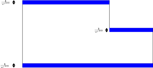
Figure 5.1. The bands are $\mathbb{M}\backslash U$

In our construction for any $(x,y)\in U$,

$$\mathtt{r}_{n}(x,y)=h_{n}(x),$$

with $h_{n}$ the functions in the one dimensional example in Section 4. This means that for any $(x,y)\in U,$

$$\mathfrak{h}_{y}(x)=\mathfrak{h}_{\underline{\epsilon}}(x).$$

We now will proceed to specify the construction of $\mathfrak{h}_{y}(x)$ for $(x,y)\in\mathbb{M}\backslash U$.

The first step is to do a coupling on the horizontal lines which roughly tells us where is the break that the problem that although $\left(x,y\right)$ is the same point in $\mathbb{M}_{\sim}$ as $\left(\hat{x},\hat{y}\right)$,

$$\left(\mathfrak{h}_{\underline{\epsilon}}(x),y\right)\neq\left(\mathfrak{h}_{\underline{\epsilon}}\left(\hat{x}\right),\hat{y}\right).$$

For example consider the case $x=1/\varphi^{3}$, $y=\frac{\varphi^{2}}{\varphi+2}$ and $\hat{x}=1/\varphi$, $\hat{y}=-\frac{\varphi}{\varphi+2}$. The point $\frac{1}{\varphi}$ is a fixed point for $\mathfrak{h}_{\underline{\epsilon}}$ meaning $\mathfrak{h}_{\underline{\epsilon}}\left(1/\varphi\right)=1/\varphi$. Since $\mathfrak{h}_{\underline{\epsilon}}\left(1/\varphi^{3}\right)=\frac{\lambda_{1}}{\varphi\left(1+\lambda_{1}\varphi\right)}\neq\frac{1}{\varphi^{3}}$ we get

$$\left(\mathfrak{h}_{\underline{\epsilon}}(x),y\right)\neq\left(\mathfrak{h}_{\underline{\epsilon}}\left(\hat{x}\right),\hat{y}\right)=\left(\hat{x},\hat{y}\right).$$

However if we took care that $\frac{1}{\varphi^{3}}$ is a fixed point for $\mathfrak{h}_{y}$ then we will have the desired equality. It turns out that the correct way to do this will be by setting $h_{1,y}|_{\left[0,1/\varphi^{3}\right)}=h_{2,y}|_{\left[0,1/\varphi^{3}\right)}=Id|_{\left[0,1/\varphi^{3}\right)}$ and to start perturbing (similarly as in the definition of $h_{n}$ from the previous Section) from $n\geq 3$. In general we will have a decomposition of the horizontal lines of $\partial\mathbb{M}$ to $\left\{V_{i}\right\}_{i=1}^{\infty}$ and we will start perturbing at $V_{i}$ from $n\geq i+1$.

To be more precise the Horizontal boundary consists of the lines $[0,1/\varphi)\times\left\{\varphi^{2}/\left(\varphi+2\right)\right\}$, $[1/\varphi,1)\times\left\{1/\left(\varphi+2\right)\right\}$ and $\mathbb{T}\times\left\{-\varphi/\left(\varphi+2\right)\right\}$. We look at a countable partition of the horizontal lines $\partial\mathbb{M}$ which are identified by $\sim$ and couple them in a time $T\in\mathbb{N}$ such that in the symbolic space on $\mathbb{T}$, the move $w(T)_{T}\to 1$ is possible for both pieces identified.

5.1.1. The horizontal subsegments of $\partial\mathbb{M}$ and their coupling time:

1. $V_{1}:=\left[0,1/\varphi^{2}\right)\times\left\{-\frac{\varphi}{\varphi+2}\right\}\sim\left[1/\varphi,1\right)\times\left\{\frac{1}{\varphi+2}\right\}$. In this case $[0,1/\varphi^{2})=C_{[1]_{1}^{1}}$ and $\left[1/\varphi,1\right)=C_{[2]_{1}^{1}}$ and $T\left(V_{1}\right)=2$.

2. $V_{2}:=\left[0,1/\varphi^{3}\right)\times\left\{\frac{\varphi^{2}}{\varphi+2}\right\}\sim\left[1/\varphi^{2},1/\varphi\right)\times\left\{-\frac{\varphi}{\varphi+2}\right\}$. Here $[0,1/\varphi^{3})=C_{[11]_{1}^{2}}$ and $\left[1/\varphi^{2},1/\varphi\right)=C_{[32]_{1}^{2}}$ and $T\left(V_{2}\right)=3$.

3. $V_{3}:=\left[1/\varphi^{3},1/\varphi^{2}\right)\times\left\{\frac{\varphi^{2}}{\varphi+2}\right\}\sim\left[1/\varphi,1/\varphi+1/\varphi^{4}\right)\times\left\{-\frac{\varphi}{\varphi+2}\right\}$. Here $[1/\varphi,1/\varphi^{2})=C_{[132]_{1}^{3}}$ and $\left[1/\varphi,1/\varphi+1/\varphi^{4}\right)=C_{[211]_{1}^{3}}$ and $T\left(V_{3}\right)=4$.

4. $V_{4}:=\left[1/\varphi^{2},1/\varphi^{2}+1/\varphi^{5}\right)\times\left\{\frac{\varphi^{2}}{\varphi+2}\right\}\sim\left[1/\varphi+1/\varphi^{4},1/\varphi+1/\varphi^{3}\right)\times\left\{-\frac{\varphi}{\varphi+2}\right\}$. Here $C_{[3211]}=\left[1/\varphi^{2},1/\varphi^{2}+1/\varphi^{5}\right)$ and $C_{[2132]}=\left[1/\varphi+1/\varphi^{4},1/\varphi+1/\varphi^{3}\right)$.

5. For general $j>4$, $V_{j}:=C_{\left[{\bf w}(j)\right]_{1}^{j}}\times\left\{\frac{\varphi^{2}}{\varphi+2}\right\}\sim C_{\left[\tilde{{\bf w}}(j)\right]_{1}^{j}}\times\left\{-\frac{\varphi}{\varphi+2}\right\}$ where ${\bf w}(j),\tilde{{\bf w}}(j)$ are the following words of length $j$,

   $${\bf w}(j) = \begin{cases}32\cdots 32132&j\ \text{odd}\\ 32\cdots 3211,&j\ {\rm\text{even}}\end{cases}$$

   $$\tilde{{\bf w}}(j) = \begin{cases}23\cdots 23211,&j\ \text{odd}\\ 23\cdots 232132&j\ \text{even}.\end{cases}$$

   As is expected for all $j\geq 2$, $T\left(V_{j}\right)=j-1$. The following is immediate from the definition.

Claim 14.

For any $j\geq 2$,

$$\tilde{f}\left(V_{j}\right)=V_{j-1},$$

and

$$\tilde{f}\left(V_{1}\right)=[0,1/\varphi)\times\{\frac{1}{\varphi+2}\}\subset U.$$

5.1.2. Definition of the perturbation maps $h_{n,y}$:

For $w\in\Sigma_{{\bf A}}$ and $n\in\mathbb{N}$, we write again $C_{[w]_{1}^{n}}:=\left[\underline{x}_{n}(w),\bar{x}_{n}(w)\right)$. Let

$${\bf u}(x,y):=\begin{cases}\min\left\{\frac{\varphi^{2}}{\varphi+2}-y,y+\frac{\varphi}{\varphi+2}\right\},&0\leq x\leq\frac{1}{\varphi}\\ \min\left\{\frac{1}{\varphi+2}-y,y+\frac{\varphi}{\varphi+2}\right\}&\frac{1}{\varphi}\leq x\leq 1\end{cases}$$

be the minimal distance of $(x,y)$ to the horizontal lines of $\partial\mathbb{M}$. In addition we will write ${\bf{\bf y}}(x,y):\mathbb{M}\to\left\{-\frac{\varphi}{\varphi+2},\frac{1}{\varphi+2},\frac{\varphi^{2}}{\varphi+2}\right\}$ to be the value so that

$${\bf u}(x,y)=\left|{\bf y}(x,y)-y\right|.$$

Under that notation $(x,{\bf y}(x,y))$ is the closest point to $(x,y)$ in the horizontal boundary. Let $(x,y)\in\mathbb{M}_{\sim}$.

Case 1 $(x,y)\in U$: we do the regular construction as in Section 4. That is for any $N_{t}<n<M_{t}$, $h_{n}$ is the identity. For any $M_{t}<n\leq N_{t}$, if $w_{n}=1$ then $h_{n}|_{H_{n-1}\left(C_{[w]_{1}^{n}}\right)}$ is a rescaling of $\psi_{t}$ to the interval $H_{n-1}\left(C_{[w]_{1}^{n}}\right)$ and if $w_{n}\neq 1$ then $h_{n}|_{H_{n-1}\left(C_{[w]_{1}^{n}}\right)}$ is the identity. If for some $t$, $n=M_{t}$ then $\left.h_{M_{t}}\circ H_{M_{t}-1}\right|_{C_{[w]_{1}^{M_{t}}}}$ is the distribution correction function in the construction. Finally we set

$$\mathtt{r}_{n}(x,y)=h_{n,y}(x):=h_{n}(x)$$

and

$$K_{n,y}(x):=h_{n,y}\circ h_{n-1,y}\circ\cdots\circ h_{1,y}(x)=H_{n}(x).$$

Case 2, $(x,y)\notin U$: In this case ${\bf u}\left(x,y\right)<\frac{1}{\varphi^{10}}$. Let $(x,{\bf y}(x,y))\in\partial\mathbb{M}$ be the closest point on the horizontal lines of $\partial\mathbb{M}$ to $(x,y)$. Let ${\bf j}(x,y)\in\mathbb{N}$ be the integer so that

$$\left(x,{\bf y}(x,y)\right)\in V_{{\bf j}(x,y)}.$$

This means that either $x\in C_{\left[{\bf w}(j)\right]_{1}^{j}}$ (if $x\leq 1/\varphi)$ or $x\in C_{\left[\tilde{{\bf w}}(j)\right]_{1}^{j}}$ ($1/\varphi\leq x<1$). We will define the construction for $x\in C_{\left[{\bf w}(j)\right]_{1}^{j}}$, the other case being similar. First we define for any $x\in C_{\left[{\bf w}(j)\right]_{1}^{j}}$,

$$K_{{\bf j}(x,y),{\bf y}(x,y)}(x)=x.$$

Then for any $(x,y)\in\mathbb{M}\backslash U$ such that $x\in C_{\left[{\bf w}({\bf j})\right]_{1}^{{\bf j}}}$ we set

$$K_{{\bf j},y}(x) := \left(H_{{\bf J}}(x)-x\right)\left[3\varphi^{20}\left({\bf u}(x,y)\right)^{2}-2\varphi^{30}{\bf u}(x,y)^{3}\right]+x$$

For $n>{\bf j}(x,y)$, assume we have defined for all ${\bf j}<k<n$, $h_{k,y}:=\mathtt{r}_{k}\left(\cdot,y\right)$ and $x\in C_{[w]_{1}^{n}}\subset C_{\left[{\bf w}({\bf j})\right]_{1}^{{\bf j}}}$. We set

$$K_{n-1,y}|_{C_{[w]_{1}^{n}}}=h_{n-1,y}\circ\cdots h_{{\bf j}+1,y}\circ K_{{\bf j},y}(x),$$

and

$$\mathfrak{l}_{n}(y,w):=m_{\mathbb{T}}\left(K_{n-1,y}\left(C_{[w]_{1}^{n}}\right)\right)=K_{n-1,y}\left(\bar{x}_{n}\left(w)\right)\right)-K_{n-1,y}\left(\underline{x}_{n}\left(w)\right)\right).$$

If $w_{n}\neq 1$ or $N_{t}<n<M_{t}$ for some $t\in\mathbb{N}$, then for all $x\in K_{n-1,y}\left(C_{[w]_{1}^{n}}\right)$, $\mathtt{r}_{n}(x,y):=x$. If $w_{n}=1$ and $M_{t}<n\leq N_{t}$ and ${\bf j}<n$ then

$$\mathtt{r}_{n}(x,y):=K_{n-1,y}\left(\underline{x}_{n}(w)\right)+\mathfrak{l}_{n}(y,w)\psi_{t}\left(\frac{x-K_{n-1,y}\left(\underline{x}_{n}(w)\right)}{\mathfrak{l}_{n}(y,w)}\right).$$

Finally if $j\leq M_{t}=n$ then $r_{M_{t},y}$ is the distribution correction function with $H_{M_{t}-1}$ replaced by $K_{M_{t}-1,y}$.

Remark 15.

The 2 variable function

$$\mathtt{q}_{{\bf J}}(x,{\bf u}):=\left(H_{{\bf J}}(x)-x\right)\left[3\varphi^{20}{\bf u}^{2}-2\varphi^{30}{\bf u}^{3}\right]+x$$

was chosen because of it’s following properties:

1. $\mathtt{q}_{{\bf J}}\left(x,\varphi^{-10}\right)=H_{{\bf J}}\left(x\right)$ and $\mathtt{q}_{{\bf J}}(x,0)=x$. This means that for $y\in\partial\mathbb{M}$, $\mathtt{r}_{n}(x,y)=x$ and therefore $K_{{\bf j},y}$ interpolates between the identity map and $H_{{\bf J}}|_{C_{\left[{\bf w}({\bf j)}\right]_{1}^{{\bf j}}}}$.

2. A consequence of the previous property is that $\frac{\partial\mathtt{q}_{{\bf j}}}{\partial x}\left(x,0\right)=1$ and $\frac{\partial\mathtt{q}_{{\bf J}}}{\partial x}\left(x,\varphi^{-10}\right)=\frac{\partial H_{{\bf J}}}{\partial x}\left(x\right)$. This is needed in order that $\frac{\partial K_{{\bf J},y}}{\partial x}$ will be continuous in $y$.

3. $\frac{\partial\mathtt{q}_{{\bf J}}}{\partial u}\left(x,0\right)=\frac{\partial\mathtt{q}_{{\bf J}}}{\partial u}\left(x,\varphi^{-10}\right)=0$ which is necessary for continuity of $\frac{\partial K_{{\bf j},y}}{\partial y}$.

4. $\sup_{0\leq z\leq\varphi^{-10}}\left|\frac{\partial\mathtt{q}_{{\bf j}}}{\partial u}(x,z)\right|=\frac{3}{2}\varphi^{10}\left|H_{{\bf j}}(x)-x\right|$. We will show that the right hand side is uniformly exponentially small when ${\bf j\to\infty}$. The control of the derivatives in the $y$ direction is to our opinion the hardest part in this section.

The idea behind this construction can be summarized as follows: For a fixed $(x,y)$ which is close enough to the horizontal segment on the boundary we first look at the coupling time of the interval which contains the point closest to $(x,y)$ on the boundary. On the boundary we start to apply the rescaling after the coupling time to ensure that the resulting map will be a map of $\mathbb{M}_{\sim}$ (respects the equivalence relation). Inside $U$ we just start perturbing from the start and in what remains we do an interpolation using $q_{{\bf J}}$, of the map on the boundary and the map on $U$.

5.1.3. Definition of $\mathfrak{Z}_{N}$ and the new examples of Anosov diffeomorphisms:

Define $\mathfrak{Z}_{N}:\mathbb{M}_{\sim}\to\mathbb{M}_{\sim}$,

$$\mathfrak{Z}_{N}(x,y)=\begin{cases}\left(K_{N,-y/\varphi}\circ S\circ K_{N,y}^{-1}(x),-y/\varphi\right),&(x,y)\in R_{1}\cup R_{3}\\ \left(K_{N,-y/\varphi+\frac{\varphi}{\varphi+2}}\circ S\circ K_{N,y}^{-1}(x),-y/\varphi+\frac{\varphi}{\varphi+2}\right),&(x,y)\in R_{2}\end{cases}.$$

Remark 16.

In the construction of the previous subsection for every $n\in\mathbb{N}$, $x\in\left\{0,1/\varphi^{2},1/\varphi\right\}$ are fixed points for $h_{\underline{\epsilon},n}$ (Remark 8). This remains true for $\mathtt{r}_{n}$ in the sense that for all $y$ and $x\in\left\{0,1/\varphi^{2},1/\varphi\right\}$ , $\mathtt{r}_{n}\left(x,y\right)=\hat{r}_{n}(x,y)=x.$ This shows that $\mathfrak{Z}_{N}$ is continuous. In addition if $x$ is an endpoint of the segment $K_{n,y}\left(C_{[w]_{1}^{n}}\right)$ for some $w\in\Sigma_{{\bf A}}$ and $y$, then $\frac{\partial\mathtt{r}_{n}}{\partial x}(x,y)=1.$ This gives that $\mathfrak{Z}_{N}$ is $C^{1}$. The invariance of the Markov partition $\left\{J_{1},J_{2},J_{3}\right\}$ of $S$ under $K_{y,n}$ gives that $\mathfrak{Z}_{N}$ is one to one and onto and

$$\mathfrak{Z}_{n}^{-1}(x,y)=\begin{cases}\left(K_{n,-\varphi y}\circ\left(\left.S\right|_{J_{1}\cup J_{3}}\right)^{-1}\circ K_{n,y}^{-1}(x),-\varphi y\right),&-\frac{\varphi}{\varphi+2}\leq y\leq\frac{1}{\varphi+2}\\ \left(K_{n,-\varphi y+\varphi^{2}/(\varphi+2)}\circ\left(\left.S\right|_{J_{2}}\right)^{-1}\circ K_{n,y}^{-1}(x),-\varphi y+\frac{\varphi^{2}}{\varphi+2}\right),&\frac{1}{\varphi+2}<y\leq\frac{\varphi^{2}}{\varphi+2}\end{cases}.$$

Here $\left(S|_{J_{1}\cup J_{3}}\right)^{-1}(x):=\frac{x}{\varphi}:[0,1]\to\left[1,1/\varphi\right]$ is the inverse branch of $S$ to the segment $[0,1/\varphi]$ and $\left(\left.S\right|_{J_{2}}\right)^{-1}(x)=\frac{x+1}{\varphi}:[0,1/\varphi]\to[1/\varphi,1]$ is the inverse branch of $S$ to the segment $[1/\varphi,1]$. Since $\mathfrak{Z}_{n}^{-1}$ is $C^{1}$, $\mathfrak{Z}_{n}$ is a diffeomorphism.

Theorem 17.

The sequence $\mathfrak{Z}_{N_{t}}$ converges in the $C^{1}$ topology to a type ${\rm III}_{1}$ Anosov diffeomorphism.

The proof of this Theorem of this paper is by a series of Lemma’s. The first step is to show that $K_{N_{t},y}(x)$ converges uniformly in $\mathbb{M}$ as $t\to\infty$.

Lemma 18.

If $x\in C_{\left[{\bf w}(J)\right]_{1}^{J}}\cup C_{\left[\tilde{{\bf w}}(J)\right]_{1}^{J}}$ and $J\in\left[M_{t-1},N_{t}\right)$,

$$\left|H_{J}(x)-x\right|\leq m_{\mathbb{T}}\left(C_{[w(x)]_{1}^{J-3}}\right)\leq\varphi^{-(J-3)},$$

where $w(x)\in\left\{{\bf w}(J),\tilde{{\bf w}}(J)\right\}$ is such that $x\in C_{\left[w(x)\right]_{1}^{J}}$.

Proof.

By the form of ${\bf w}(J)\ \text{and }\tilde{{\bf w}}(J)$ one has that for all $l\leq J-3$, $w(x)_{l}\in\{2,3\}$, hence

$$H_{J-3}(x)|_{C_{[w(x)]_{1}^{J-3}}}=x.$$

Since $\underline{x}_{J-3}(w(x)),\ \bar{x}_{J-3}(w(x))$ are fixed points of $h_{j-2},h_{j-1}$ and $h_{j}$ , $H_{J}\left(C_{[w(x)]_{1}^{J-3}}\right)=C_{[w(x)]_{1}^{J-3}}$, the lemma follows. ∎

Corollary 19.

The limit

$$\lim_{n\to\infty}K_{n,y}(x)=:\mathfrak{h}_{y}(x)$$

exists uniformly in $\mathbb{M}$ and is a continuous function and the function $\mathcal{H}(x,y)=\left(\mathfrak{h}_{y}(x),y\right)$ is a homeomorphism of $\mathbb{M}_{\sim}$.

Proof.

The proof is similar to the proof of Lemma 11. First we claim that for every $n\in\mathbb{N}$,

(5.1) $$\sup_{(x,y)\in\mathbb{M}_{\sim}}\left|\mathtt{r}_{n}(x,y)-x\right|\leq\left(1.5\right)^{-n}.$$

This is true since for every $w\in\Sigma_{{\bf A}}$,

$$\mathtt{r}_{n}\left(K_{n-1,y}\left(C_{[w]_{1}^{n}}\right),y\right)=K_{n-1,y}\left(C_{[w]_{1}^{n}}\right),$$

and consequently

$$\left|\mathtt{r}_{n}(x,y)-x\right|\leq m_{{\rm\mathbb{T}}}\left(K_{n-1,y}\left(C_{[w]_{1}^{n}}\right)\right)\leq\left(\frac{\lambda_{1}^{2}}{\varphi}\right)^{-n}.\ \ \ \boxtimes\eqref{eq: r_n is uniformly close to x}$$

The last inequality follows since $\left|\frac{\partial\psi_{l}}{\partial x}\left(x\right)\right|\leq\lambda_{1}^{2}$ for every $l\in\mathbb{N}$ and thus $\left|\frac{\partial\mathtt{r}_{k}}{\partial x}\right|_{\infty}\leq\lambda_{1}^{2}.$ Proceeding as in Lemma 11, it follows that for every $y$, $\left\{K_{n,y}(x)\right\}_{n=1}^{\infty}$ is a Cauchy sequence in the uniform topology. Thus, $\mathfrak{h}_{y}(x)$ is a continuous function in $\mathbb{M}$ as it is a uniform limit of continuous functions. Notice that $\mathfrak{h}_{y}$ is a homeomorphism of the circle for $y\in\left[-\varphi/\left(\varphi+2\right),1/(\varphi+2)\right]$ or of $\left[0,1/\varphi\right]$ if $y\in\left[1/\left(\varphi+2\right),\varphi^{2}/\left(\varphi+2\right)\right]$.

It remains to show that if $\left(x,y\right)\sim\left(\hat{x},\hat{y}\right)$ (for points on $\partial\mathbb{M}$) then $\left(\mathfrak{h}_{y}(x),y\right)\sim\left(\mathfrak{h}_{\hat{y}}\left(\hat{x}\right),\hat{y}\right)$. Let $\left(x,y\right),\left(\hat{x},\hat{y}\right)\in\partial\mathbb{M}$ with $\left(x,y\right)\sim\left(\hat{x},\hat{y}\right)$. There exists ${\bf j}(x,y)\in\mathbb{N}$ such that $\left(x,y\right),\left(\hat{x},\hat{y}\right)\in V_{{\bf j}}$. Since $\left(x,y\right)\sim\left(\hat{x},\hat{y}\right)$, it follows that for every $n>{\bf j}$ and a word $w\in\Sigma_{{\bf A}}(n)$,

$$x\in C_{\left[{\bf w}({\bf j)}w\right]_{1}^{n+{\bf j}}}\ \Leftrightarrow\ \hat{x}\in C_{\left[\tilde{{\bf w}}\left({\bf j}\right)w\right]_{1}^{n+{\bf j}}}.$$

Since for all $n\leq{\bf j}$, $\mathtt{r}_{n}|_{V_{{\bf J}}}=Id_{\mathbb{T}}$, this property and the definition of $r_{n}(\cdot,\cdot)$ yields that for all $n\in\mathbb{N}$,

$$\left(K_{n,y}(x),y\right)\sim\left(K_{n,\hat{y}}\left(\hat{x}\right),\hat{y}\right).$$

The Lemma follows by taking $n\to\infty$. ∎

Denote the function of the first coordinate by $\mathfrak{z}_{n}(x,y)$. Our goal is to prove that the limit

$$\mathfrak{z}(x,y):=\lim_{t\to\infty}\mathfrak{z}_{N_{t}}(x,y)$$

exists for all $(x,y)$ and $\mathfrak{z}$ is a $C^{1}\left(\mathbb{M}_{\sim}\right)$ function with

$$1.6\leq\frac{\partial\mathfrak{z}}{\partial x}(x,y)\leq 1.7.$$

The conclusion of hyperbolicity of $\mathfrak{Z}$ will follow from a standard Lemma in the theory of Lyapunov exponents.

Lemma 20.

If in addition

$$1.6\leq\varphi\cdot\lambda_{1}^{6}\left(\prod_{t\in\mathbb{N}}\lambda_{t}^{\pm 2M_{t-1}}\right)\cdot\exp\left(\pm\sum_{t=1}^{\infty}2^{-N_{t}+4}\right)\leq 1.7$$

then $\frac{\partial\mathfrak{z}}{\partial x}$ is a continuous function in $\mathbb{M}_{\sim}$ and

$$1.6\leq\frac{\partial\mathfrak{z}}{\partial x}(x,y)\leq 1.7.$$

Remark.

The extra condition in this Lemma can easily be inserted into the inductive construction of the sequence $\left\{\lambda_{k},M_{k},N_{k},m_{k},n_{k},\epsilon_{k}\right\}_{k=1}^{\infty}$.

Proof.

Let $(x,y)\in\mathbb{M}_{\sim}$. For convenience to the reader, we will first show that $\frac{\partial\mathfrak{z}_{N_{t}}}{\partial x}(x,y)$ converges pointwise and $1.6\leq\frac{\partial\mathfrak{z}}{\partial x}(x,y)\leq 1.7$ and then argue that the convergence is in fact uniform.

Let $t\in\mathbb{N}$ and $(x,y)\in\mathbb{M}_{\sim}$ be fixed. There exists a $w=w(x)\in\Sigma_{{\bf A}}$ such that for all $t\in\mathbb{N},$ $x\in K_{N_{t},y}\left(C_{[w]_{1}^{N_{t}}}\right)$. As in the proof of Lemma 12, we write $z_{y}(x)$ to be the unique point in $C_{[w]_{1}^{N_{t}}}$ such that $x=K_{N_{t},y}\left(z_{y}(x)\right)$. Recall that

$$\mathfrak{z}_{N_{t}}(x,y) = \begin{cases}K_{N_{t},-y/\varphi}\left(\varphi K_{N_{t},y}^{-1}(x)\right),&0\leq x\leq 1/\varphi\\ K_{N_{t},-y/\varphi+\varphi/\varphi+2}\left(\varphi K_{N_{t},y}^{-1}(x)-1\right),&1/\varphi\leq x\leq 1\end{cases}$$

$$= \begin{cases}K_{N_{t},-y/\varphi}\left(Sz_{y}(x)\right),&0\leq x\leq 1/\varphi\\ K_{N_{t},-y/\varphi+\varphi/\varphi+2}\left(Sz_{y}(x)\right),&1/\varphi\leq x\leq 1\end{cases}.$$

By the chain rule, the Lemma will follow once we show that uniformly in $\left(x,y\right)\in\mathbb{M}_{\sim}$ with $0\leq x\leq 1/\varphi$,

(5.2) $$\lim_{t\to\infty}\left(\frac{\partial K_{N_{t},-y/\varphi}}{\partial x}\left(Sz_{y}(x)\right)\right)\cdot\left(\frac{\partial K_{N_{t},y}}{\partial x}\left(z_{y}(x)\right)\right)^{-1} \in \left(\frac{1.6}{\varphi},\frac{1.7}{\varphi}\right),$$

and for every $\left(x,y\right)\in\mathbb{M}_{\sim}$ with $1/\varphi\leq x\leq 1$,

$$\lim_{t\to\infty}\left(\frac{\partial K_{N_{t},-y/\varphi+\varphi/\varphi+2}}{\partial x}\left(Sz_{y}(x)\right)\right)\cdot\left(\frac{\partial K_{N_{t},y}}{\partial x}\left(z_{y}(x)\right)\right)\in\left(\frac{1.6}{\varphi},\frac{1.7}{\varphi}\right).$$

We will separate the proof for three cases: We assume that $(x,y)\in R_{1}\cup R_{3}$, equivalently $0\leq x\leq 1/\varphi$, the proof when $(x,y)\in R_{2}$ is similar and just involves changing the appearance of $-y/\varphi$ by $-y/\varphi+\varphi/(\varphi+2)$.

Case 1: $(x,y)\in U\cap\mathfrak{Z}^{-1}U$. In this case

$$\mathfrak{z}_{N_{t}}(x,y)=H_{N_{t}}\circ S\circ H_{N_{t}}^{-1}(x),$$

and the conclusion is true by Lemma 12.

Case 2: $(x,y)\in U\cap\mathfrak{Z}^{-1}U^{c}$. Firstly since $(x,y)\in U$ then $K_{n,y}(x)=H_{n}(x)$. In addition, because $\mathfrak{Z}(x,y)\notin U$ there exists $\mathbf{J\in\mathbb{N}}$ such that

$$\left[w_{2},...,w_{{\bf J}+1}\right]_{1}^{{\bf J}}=\left[{\bf w}({\bf J})\right]_{1}^{{\bf J}}\ \text{or }\left[\tilde{{\bf w}}({\bf J})\right]_{1}^{{\bf J}},$$

and consequently $w_{n}\neq 1$ for all $2\leq l<\mathbf{J}-2$. This shows that $\left.K_{n,y}\right|_{C_{[w]_{1}^{n}}}=h_{n}\circ\cdots h_{{\bf J}-2}\circ h_{1}$ and writing $z_{y}(x)\in\mathbb{T}$ for the point such that $K_{N_{t},y}\left(z_{y}(x)\right)=x$,

$$\frac{\partial K_{N_{t},y}}{\partial x}\left(z_{y}(x)\right)=\frac{\partial h_{1}}{\partial x}\left(z_{y}(x)\right)\cdot\prod_{k={\bf J}-2}^{N_{t}}\frac{\partial h_{l}}{\partial x}\left(H_{l-1}\left(z_{y}(x)\right)\right).$$

By the definition of the construction

$$\frac{\partial K_{N_{t},-y/\varphi}}{\partial x}\left(Sz_{y}(x)\right)=\prod_{l={\bf J}}^{N_{t}}\frac{\partial h_{l,-y/\varphi}}{\partial x}\left(K_{l-1,-y/\varphi}(Sz_{y}(x))\right),$$

and, here $\lambda_{t\left({\bf J}\right)}=\lambda_{k}$ if $N_{k-1}<{\bf J}\leq N_{k}$ or $1$ otherwise,

$$\left(\frac{\partial K_{N_{t},-y/\varphi}}{\partial x}\left(Sz_{y}(x)\right)\right)\cdot\left(\frac{\partial K_{N_{t},y}}{\partial x}\left(z_{y}(x)\right)\right)^{-1} = \lambda_{t\left({\bf J}\right)}^{\pm 6}\left(\frac{\partial h_{1}}{\partial x}\left(z_{y}(x)\right)\right)^{-1}{\bf\cdot I},$$

Where

$${\bf I}:=\left(\prod_{l={\bf J}}^{N_{t}}\frac{\partial h_{l,-y/\varphi}}{\partial x}\left(K_{l-1,-y/\varphi}\left(Sz_{y}(x)\right)\right)\right)\cdot\left(\prod_{l={\bf J}}^{N_{t}}\frac{\partial h_{l,y}}{\partial x}\left(H_{l}\left(z_{y}(x)\right)\right)\right)^{-1}.$$

As in the proof of Lemma 12, assuming that $\underline{\epsilon}\equiv 0$, one has that for $l\geq{\bf J}+1$, $K_{l-1,-y/\varphi}\left(Sz_{y}(x)\right)$ is to the right of the point in $1/\varphi$ proportion in $K_{l-1,-y/\varphi}\left(C_{[w_{2},...,w_{l+1}]}\right)$ if and only if $K_{l-1,y}\left(z_{y}(x)\right)$ is to the right of the point in $1/\varphi$ proportion in $K_{l,-y/\varphi}\left(C_{[w]_{1}^{l+1}}\right)$. This means that in the case $\underline{\epsilon}=0$,

$$\left(\frac{\partial h_{l-1,-y/\varphi}}{\partial x}\left(K_{l-2,-y/\varphi}(Sz_{y}(x))\right)\right)\cdot\left(\frac{\partial h_{l,y}}{\partial x}\left(K_{l-1,y}(z_{y}(x))\right)\right)^{-1}=1.$$

By proceeding with the analysis of the the bad sets as in Lemma 12 one proves that

$${\bf I}=\left(\prod_{k=t\left({\bf J}\right)}^{t}\lambda_{k}^{\pm 2M_{k-1}}\right)\exp\left(\pm\sum_{k=t\left({\bf J}\right)}^{t}2^{-N_{k}+4}\right),$$

and thus

$$\left(\frac{\partial K_{N_{t},-y/\varphi}}{\partial x}\left(Sz_{y}(x)\right)\right)\cdot\left(\frac{\partial K_{N_{t},y}}{\partial x}\left(z_{y}(x)\right)\right)^{-1} = \left[\left(\frac{\partial h_{1}}{\partial x}\left(z_{y}(x))\right)\right)^{-1}\left(\prod_{k=t\left({\bf J}\right)}^{t}\lambda_{k}^{\pm 2M_{k-1}}\right)\right.$$

$$\left.\cdot\exp\left(\pm\sum_{k=t\left({\bf J}\right)}^{t}2^{-N_{k}+4}\right)\right].$$

This shows (5.2). In fact, because

$$\lim_{s\to\infty}\left(\prod_{k=s}^{\infty}\lambda_{k}^{\pm 2M_{k-1}}\right)\exp\left(\pm\sum_{k=s}^{\infty}2^{-N_{k}+4}\right)=1,$$

the convergence is uniform as $t\to\infty$.

Case 3: $(x,y)\in U^{c}$. In this case let ${\bf\tilde{J}}\in\mathbb{N}$ be such that the closest point to $(x,y)$ on the Horizontal segments of $\partial\mathbb{M}$ is in $V_{\tilde{{\bf J}}}$. If $\tilde{{\bf J}}=1$ then $\left(Sz_{y}(x),-y/\varphi\right)\in U$. Otherwise $\left(Sz_{y}(x),-y/\varphi\right)$ is in $U^{c}$ and the closest point to it on the Horizontal segments of $\partial\mathbb{M}$ is in $V_{\tilde{{\bf J}}-1}$. Consequently

$$\left(\frac{\partial K_{N_{t},-y/\varphi}}{\partial x}\left(Sz_{y}(x)\right)\right)\cdot\left(\frac{\partial K_{N_{t},y}}{\partial x}\left(z_{y}(x)\right)\right)^{-1} = \left(\prod_{l={\bf\tilde{J}}-1}^{N_{t}}\frac{\partial h_{l,-y/\varphi}}{\partial x}\left(K_{l-1,-y/\varphi}\left(Sz_{y}(x)\right)\right)\right)$$

$$\cdot\left(\prod_{l={\bf\tilde{J}}}^{N_{t}}\frac{\partial h_{l,y}}{\partial x}\left(K_{l-1,y}\left(z_{y}(x)\right)\right)\right)^{-1}.$$

Similarly as in case 2, one has

$$\left(\frac{\partial K_{N_{t},-y/\varphi}}{\partial x}\left(Sz_{y}(x)\right)\right)\cdot\left(\frac{\partial K_{N_{t},y}}{\partial x}\left(z_{y}(x)\right)\right)^{-1}=\lambda_{t\left({\bf\tilde{J}}\right)}^{\pm 2}\left(\prod_{k=t\left(\tilde{{\bf J}}\right)}^{t}\lambda_{k}^{\pm 2M_{k-1}}\right)\exp\left(\pm\sum_{k=t\left(\tilde{{\bf J}}\right)}^{t}2^{-N_{k}+4}\right)$$

and the convergence is uniform. ∎

5.1.4. Proving differentiability in the $y$-direction.

Again we will prove differentiability in the $y$ direction for $(x,y)\in R_{1}\cup R_{3}$. The idea of the proof here is as follows. If $(x,y)\in U$ then $K_{n,\tilde{y}}(x)=H_{\underline{\epsilon},n}(x)$ for all $\tilde{y}$ in a neighborhood of $(x,y)$, hence $\frac{\partial K_{n,y}}{\partial y}(\cdot)\equiv 0$. Otherwise, for $(x,y)\in\mathbb{M}\backslash U$, $K_{{\bf j}(x,y)-2,\tilde{y}}(x)=x$ and the first (major) change between $K_{n,y}(x)$ and $K_{n,\tilde{y}}(x)$ appears at time $n={\bf j}(x,y)$. We will show that for our construction the $y$ derivative of $K_{n,y}(x)$ can be bounded above by a (bounded) constant times $\frac{\partial K_{{\bf j}(x,y),y}(x)}{\partial y}$, the uniform convergence of $\partial\mathfrak{z}_{n}/\partial y$ will follow from the chain rule and simple arithmetic.

The following notation will be used in this subsection. Usually we will consider $x\in[0,1/\varphi$] and work constantly with a fixed $w\in\Sigma_{{\bf A}}$ such that $x\in C_{[w]_{1}^{n}}$ for all $n\in\mathbb{N}$. If that is the case we will write $\left[\underline{x}_{n},\bar{x}_{n}\right)$ to denote $C_{[w]_{1}^{n}}$.

For $-\frac{\varphi}{\varphi+2}\leq y\leq\frac{\varphi^{2}}{\varphi+2}$ and $n\geq{\bf N}(y)$, let ${\rm BS}(n,w,y)\subset C_{[w]_{1}^{n}}$ to be the bad set as in the proof of Lemma 12 with $h_{n}^{\prime}\circ H_{n}$ replaced by $\left(\frac{\partial r_{n,y}}{\partial x}\right)\circ K_{n-1,y}$.

For an $w\in\Sigma_{{\bf A}}$ we denote by $w_{1}^{n}=w_{1}w_{2}\cdots w_{n}$ the finite word derived by $w$ up to time $n$. Given a finite word $w_{1}^{n}$, $[w_{1}^{n}]$ denotes the $n$-periodic word defined by $w_{1}^{n}$. Finally given two words $w$ and $\tilde{w}$ (in which case $w$ is a finite word), the word $w\tilde{w}$ denotes the concatenation of $w$ and $\tilde{w}$.

Recall the definition of $K_{{\bf j}(x,y),y}(x)=\mathtt{r}_{{\bf j}(x,y)}\left(x,y\right)$ which is defined by

$$\mathtt{r}_{{\bf j}(x,y)}(x,y):=\left(H_{{\bf j}(x,y)}(x)-x\right)\mathscr{P}(x,y)+x,$$

where

$$\mathscr{P}(x,y)=\left[3\varphi^{20}\left({\bf u}(x,y)\right)^{2}-2\varphi^{30}{\bf u}(x,y)^{3}\right].$$

In the following proof if ${\bf j}(x,y)={\bf J}$ we will need a different definition of the bad set for $n={\bf J}$. Let

$$\mathbb{BS}\left({\bf J}\right):=\begin{cases}{\rm BS}\left({\bf J}-2,{\bf w}\left({\bf J}\right)\right),&{\bf J}\ odd\\ {\rm BS}\left({\bf J}-1,{\bf w}\left({\bf J}\right)\right)\cup{\rm BS}\left({\bf J},{\bf w}\left({\bf J}\right)\right)&{\bf J}\ even\end{cases}$$

if $(x,y)\in R_{1}\cup R_{3}$ (For $(x,y)\in R_{2}$ change the odd to even and even to odd).

Lemma 21.

Assume that $M_{t}\leq{\bf j}\leq N_{t+1}$, and $x\in C_{[w]_{1}^{N_{t+1}}}$. If $x\notin\mathbb{BS}\left({\bf J}\right)$, for every ${\bf j<}n\leq N_{t+1}$, there exists $0\leq\beta_{n}(x)\leq\varphi$ such that for every $(x,y)$ with ${\bf j}\left(x,y\right)={\bf j}$,

$$K_{n,y}(x)=K_{n,y}\left(\underline{x}_{n}\right)+\beta_{n}(x)l_{n}\left(y,w\right),$$

in addition $\beta_{N_{t+1}}(x)$ is continuous in $x$.

Proof.

Let $(x,y)\in\left(\mathbb{M}\backslash U\right)\cup\left(R_{1}\cup R_{3}\right)$ so that ${\bf j}(x,y)={\bf j}$ (the case $(x,y)\in R_{2}$ is similar). The proof is by induction on $n$. Since $x\notin\mathbb{BS}\left({\bf J}\right)$, $\underline{x}_{{\bf J}+1}\in\left\{\underline{x}_{{\bf J}},\underline{x}_{{\bf J}}+\varphi^{-1}\left(\bar{x}_{{\bf J}}-\underline{x}_{{\bf J}}\right)\right\}$ and

$${\bf w}\left({\bf J}\right)=\begin{cases}32\cdots 32132,&{\bf J}\ \text{odd}\\ 32\cdots 3211,&{\bf J}\ \text{even}\end{cases},$$

it follows that if ${\bf J}$ is even then by property (3) of $\psi_{t}$,

$$H_{{\bf J}}\left(x\right)-H_{{\bf J}}\left(\underline{x}_{{\bf J}+1}(w)\right) = \begin{cases}\left(\varphi\psi_{t+1}(1/\varphi)\right)^{2}\left(x-\underline{x}_{{\bf{\bf J}}+1}\right),&w_{{\bf{\bf J}}+1}=1\\ \left(\varphi\psi_{t+1}(1/\varphi)\right)\left(\varphi^{2}\left(1-\psi_{t+1}\left(1/\varphi\right)\right)\right)\left(x-\underline{x}_{{\bf J}+1}\right),&w_{{\bf N+1}}=3\end{cases}$$

$$= \frac{P_{{\bf J}-1}\left(w_{{\bf J}-1},w_{{\bf J}}\right)}{{\rm Q}\left(w_{{\bf J}},w_{{\bf J}+1}\right)}\frac{P_{{\bf J}}\left(w_{{\bf J}},w_{{\bf J}+1}\right)}{{\rm Q}\left(w_{{\bf J}},w_{{\bf J}+1}\right)}\left(x-\underline{x}_{{\bf J}+1}\right)$$

$$:= b\left(x-\underline{x}_{{\bf J+1}}\right).$$

and if ${\bf J}$ is odd then

$$H_{{\bf J}}\left(x\right)-H_{{\bf J}}\left(\underline{x}_{{\bf J}+1}\right) = \varphi^{2}\left(1-\psi_{t+1}\left(1/\varphi\right)\right)\left(x-\underline{x}_{{\bf J}+1}\right)$$

$$= \frac{P_{{\bf J}-2}\left(w_{{\bf J}-2},w_{{\bf J}-1}\right)}{{\rm Q}\left(w_{{\bf J}-2},w_{{\bf J}-1}\right)}\left(x-\underline{x}_{{\bf J}+1}\right)$$

$$:= b\left(x-\underline{x}_{{\bf J+1}}\right).$$

It then follows that

$$K_{{\bf J},y}(x)-K_{{\bf J},y}\left(\underline{x}_{{\bf J}+1}\right): = \mathtt{r}_{{\bf J}}\left(x,y\right)-\mathtt{r}_{{\bf J}}\left(\underline{x}_{{\bf J}+1},y\right)$$

$$= \left(x-\underline{x}_{{\bf J}+1}\right)\left[\left(b-1\right)\mathscr{P}(x,y)+1\right],$$

and

$$\mathfrak{l}_{{\bf j+1}}(y,w) := K_{{\bf j},y}\left(\bar{x}_{{\bf J}+1}\right)-K_{{\bf j},y}\left(\underline{x}_{{\bf j+1}}\right)$$

$$= \left(\bar{x}_{{\bf j}+1}-\underline{x}_{{\bf J}+1}\right)\left[\left(b-1\right)\mathscr{P}(x,y)+1\right].$$

This implies that

(5.3) $$\frac{K_{{\bf J},y}\left(x\right)-K_{{\bf J},y}\left(\underline{x}_{{\bf J}+1}\right)}{\mathfrak{l}_{{\bf J}+1}(y,w)}=\frac{x-\underline{x}_{{\bf J}+1}}{\bar{x}_{{\bf J}+1}-\underline{x}_{{\bf J+1}}}.$$

Therefore

$$K_{{\bf J}+1,y}(x)=K_{{\bf J+1},y}\left(\underline{x}_{{\bf J}+1}\right)+\underset{:=\beta_{{\bf j}}(x)}{\underbrace{\psi_{t+1}\left(\frac{x-\underline{x}_{{\bf j+1}}}{\bar{x}_{{\bf J}+1}-\underline{x}_{{\bf j+1}}}\right)}}\mathfrak{l}_{{\bf J}+1}\left(y,w\right)$$

and the base of induction is proved.

For the inductive step notice that if the conclusion of the Lemma is true for $n\in\mathbb{N}$, then

$$\frac{K_{n,y}(x)-K_{n,y}\left(\underline{x}_{n+1}\right)}{\mathfrak{l}_{n+1}(y,w)}=\frac{\beta_{n}(x)-\beta_{n}\left(\underline{x}_{n+1}\right)}{\beta_{n}\left(\bar{x}_{n+1}\right)-\beta_{n}\left(\underline{x}_{n+1}\right)}$$

does not depend on $y.$ The conclusion then follows for $n+1$ with

$$\beta_{n+1}(x):=\psi_{t+1}\left(\frac{\beta_{n}(x)-\beta_{n}\left(\underline{x}_{n+1}\right)}{\beta_{n}\left(\bar{x}_{n+1}\right)-\beta_{n}\left(\underline{x}_{n+1}\right)}\right)$$

and the continuity of $\beta_{n+1}$ follows from the continuity of $\beta_{n}$ and $\psi_{t+1}$. ∎

The last lemma shows the importance of knowing how $\frac{\partial\mathfrak{l}_{n}}{\partial y}$ decays when ${\bf N}(y)<n\leq N_{t+1}$. We will now show that it is exponential in $n$.

Lemma 22.

Let $M_{t}\leq{\bf j}<n\leq N_{t+1}$, a $w\in\Sigma_{{\bf A}}$ with $w_{1}^{{\bf j}}={\bf w(j)}$ and $-\frac{\varphi}{\varphi+2}\leq y\leq\frac{\varphi^{2}}{\varphi+2}$, then

$$\left|\frac{\partial\mathfrak{l}_{n}}{\partial y}(y,w)\right|\leq(1.6)^{{\bf j}-n}\left|\frac{\partial l_{{\bf j}}}{\partial y}(y,w)\right|$$

and

$$\left|\frac{\partial\mathfrak{l}_{{\bf j}+1}}{\partial y}(y,w)\right|\lesssim(1.6)^{-{\bf j}}.$$

Proof.

We assume $\left(\underline{x}_{N_{t+1}},y\right)\notin\partial U$, the proof for the case $\left(\underline{x}_{N_{t+1}},y\right)\in\partial U$ is similar. In this case for small $|h|$, $\left(\underline{x}_{N_{t+1}},y+h\right)\in U^{c}$.

Since $\bar{x}_{N_{t+1}}(w)$ is not in the bad set $\mathbb{BS}\left({\bf j}(x,y)\right)$, it follows from (5.3) that for small $|h|$,

$$\frac{m_{{\rm\mathbb{T}}}\left(K_{{\bf j},y+h}\left(C_{[w]_{1}^{N_{t+1}}}\right)\right)}{m_{\mathbb{T}}\left(K_{{\bf j},y+h}\left(C_{[w]_{1}^{{\bf j}+1}}\right)\right)}: = \frac{K_{{\bf j},y+h}\left(\bar{x}_{N_{t+1}}\right)-K_{{\bf j},y+h}\left(\underline{x}_{N_{t+1}}\right)}{K_{{\bf j},y+h}\left(\bar{x}_{{\bf j}+1}\right)-K_{{\bf j},y+h}\left(\underline{x}_{{\bf j}+1}\right)}$$

$$= \frac{\bar{x}_{N_{t+1}}-\underline{x}_{N_{t+1}}}{\bar{x}_{{\bf j}+1}-\underline{x}_{{\bf j}+1}}$$

$$= \frac{m_{{\rm\mathbb{T}}}\left(C_{[w]_{1}^{N_{t}+1}}\right)}{m_{\mathbb{T}}\left(C_{[w]_{1}^{{\bf j}+1}}\right)}.$$

It then follows by definition of $h_{n,y}$ for $n>{\bf j}$ that for $|h|$ small,

$$\mathfrak{l}_{N_{t+1}}(y+h,w)=l_{{\bf j}+1}(y+h,w)\prod_{k={\bf j}+1}^{N_{t+1}}P_{k}\left(w_{k},w_{k+1}\right),$$

hence

$$\frac{\mathfrak{l}_{N_{t+1}}(y+h,w)}{\mathfrak{l}_{N_{t+1}}(y,w)}=\frac{\mathfrak{l}_{{\bf j}+1}(y+h,w)}{\mathfrak{l}_{{\bf j}+1}(y,w)}.$$

This yields that

$$\mathfrak{l}_{N_{t+1}}(y+h,w)-\mathfrak{l}_{N_{t+1}}(y,w)=\frac{\mathfrak{l}_{N_{t+1}}(y,w)}{\mathfrak{l}_{{\bf j}(x,y)+1}(y,w)}\left[\mathfrak{l}_{{\bf j}(x,y)+1}(y+h,w)-\mathfrak{l}_{{\bf j}(x,y)+1}(y,w)\right],$$

dividing by $h$ and taking limit $h\to 0$ we get

$$\left|\frac{\partial\mathfrak{l}_{N_{t+1}}(y,w)}{\partial y}\right|=\frac{\mathfrak{l}_{N_{t+1}}(y,w)}{\mathfrak{l}_{{\bf j}+1}(y,w)}\left|\frac{\partial\mathfrak{l}_{{\bf j}+1}(y,w)}{\partial y}\right|\leq(1.6)^{{\bf j}-N_{t+1}}\left|\frac{\partial\mathfrak{l}_{{\bf j}+1}(y,w)}{\partial y}\right|.$$

The last inequality follows from, for all $N_{t}\leq{\bf j}<n\leq N_{t+1}$,

$$\prod_{k={\bf j}}^{n-1}P_{k}\left(w_{k},w_{k+1}\right)\leq\left(\frac{\lambda_{t+1}\varphi}{1+\lambda_{t+1}\varphi}\right)^{{\bf j}-n}\leq\left(\frac{\lambda_{t+1}}{\varphi}\right)^{{\bf j}-n}<(1.6)^{{\bf j}-n}.$$

For the proof of the second part notice that for $x\in\left\{\underline{x}_{{\bf j}},\bar{x}_{{\bf j}}\right\}$,

$$\left|\frac{\partial K{}_{{\bf j},y}}{\partial y}(x)\right| = \left|\frac{\partial\mathtt{r}{}_{{\bf j}}}{\partial y}(x,y)\right|$$

$$\leq \left|\frac{\mathtt{\partial}\mathscr{P}}{\partial y}(x,y)\right|\left|H_{\underline{\epsilon},{\bf j}}(x)-x\right|$$

$$\leq \frac{3}{2}\varphi^{10}\left|m\left(C_{[w]_{1}^{{\bf j}-2}}\right)\right|\leq\frac{3}{2}\varphi^{12}\varphi^{-{\bf j}}\leq\frac{1}{2}(1.62)^{-{\bf j}},$$

for all large ${\bf j}$. Thus (recall $\mathfrak{l}_{{\bf j}+1}(y,w)=\mathtt{r}{}_{{\bf j}(x,y)}\left(\bar{x}_{{\bf j}+1}\right)-\mathtt{r}{}_{{\bf j}}\left(\underline{x}_{{\bf j}+1}\right)$)

$$\left|\frac{\partial\mathfrak{l}_{{\bf j}+1}}{\partial y}(y,w)\right| \leq (1.6)^{-{\bf j}},\ \ \text{for all large}\ {\bf j.}$$

∎

Lemma 21 shows that if $x\in C_{[{\bf w}\left({\bf j}\right)]_{1}^{n}}$ is not in $x\in\mathbb{BS}\left({\bf j}\right)$ then the $y$- derivative of $K_{N_{t+1},y}(x)$ (here $t$ is the number such that $N_{t}<{\bf j}<N_{t+1}$) is controlled by the derivative on a finite collection of points plus the evolution of the lengths of the intervals. We would like to point out that there is actually no bad set if $N_{t}<{\bf j}\leq M_{t}$ because then $K_{{\bf j},y}|_{C_{[{\bf w}\left({\bf j}\right)]_{1}^{{\bf j}}}}=id_{\mathbb{T}}$. This idea will be reiterated with a slight modification for the derivatives $\partial K_{n,y}/\partial y$ for $M_{s}<n<N_{s}$ where $M_{s}>{\bf j}(x,y)$.

For points in the bad set we will apply a correction point procedure which we call the $x$-delta method. Assume that $x\in\mathbb{BS}\left({\bf j}\right)$. For $\Delta$-small (so that $(x,y\pm\Delta)\in U^{c})$) there exists a unique ${\bf x}\left(\Delta\right)$ such that

(5.5) $$\frac{K_{{\bf j}(x,y),y+\Delta}({\bf x}\left(\Delta\right))-K_{{\bf j}(x,y),y+\Delta}\left(\underline{x}_{{\bf j}(x,y)+1}\right)}{\mathfrak{l}_{{\bf j}(x,y)+1}(y+\Delta,w)}=\frac{K_{{\bf j}(x,y),y}(x)-K_{{\bf j}(x,y),y}\left(\underline{x}_{{\bf j}(x,y)+1}\right)}{\mathfrak{l}_{{\bf j}(x,y)+1}(y,w)}.$$

We will use Lemma 22 to obtain a first order approximation for ${\bf x}\left(\Delta\right)$ when $\Delta$ is small.

In the next Lemma, if $M_{t}<{\bf j}+1<N_{t+1}$ $\beta_{{\bf j}+1}(x):=\psi_{t+1}\left(\frac{K_{{\bf j},y}(x)-K_{{\bf j},y}\left(\underline{x}_{{\bf j}+1}\right)}{\mathfrak{l}_{{\bf j}+1}(y,w)}\right)$ and for $M_{t}<{\bf j}+1<n\leq N_{t+1}$

$$\beta_{n+1}(x):=\psi_{t+1}\left(\frac{\beta_{n}(x)-\beta_{n}\left(\underline{x}_{n+1}\right)}{\beta_{n}\left(\bar{x}_{n+1}\right)-\beta_{n}\left(\underline{x}_{n+1}\right)}\right).$$

Lemma 23.

Assume that $M_{t}\leq{\bf j}\leq N_{t+1}$, and $x\in C_{[w]_{1}^{N_{t+1}}}$ with $w_{1}^{{\bf j}}={\bf w}\left({\bf j}\right)$. The following holds:

(i) For every $y$ so that ${\bf j}\left(x,y\right)={\bf j}$ and $\Delta$ so that $(x,y\pm\Delta)\in\mathbb{M}\backslash U$,

$$K_{N_{t+1},y+\Delta}\left({\bf x}\left(\Delta\right)\right)=K_{N_{t+1},y+\Delta}\left(\underline{x}_{N_{t+1}}\right)+\beta_{N_{t+1}}(x)l_{N_{t+1}}\left(y+\Delta,w\right),$$

(ii) $\left|{\bf x}\left(\Delta\right)-x\right|\leq 4(1.6)^{-N_{t+1}}\Delta+o\left(\Delta\right)$ as $\Delta\to 0$.

Proof.

(i) This is the same as the proof of Lemma 21 by using (5.5) as the starting point.

(ii) If $x\notin\mathbb{BS}\left({\bf j}\right)\cap C_{[w]_{1}^{N_{t}}}$ then by Lemma 21, ${\bf x}\left(\Delta\right)=x$. Since $\underline{x}_{N_{t+1}}\notin\mathbb{BS}\left({\bf j}\right)$,

$$\frac{K_{{\bf j},y+\Delta}\left(\underline{x}_{N_{t+1}}\right)-K_{{\bf j},y+\Delta}\left(\underline{x}_{{\bf j}(x,y)+1}\right)}{\mathfrak{l}_{{\bf j}+1}(y+\Delta,w)} = \frac{\underline{x}_{N_{t+1}}-\underline{x}_{{\bf j}(x,y)+1}}{\overline{x}_{{\bf j}+1}-\underline{x}_{{\bf j}+1}}$$

$$= \frac{K_{{\bf j},y}\left(\underline{x}_{N_{t+1}}\right)-K_{{\bf j},y}\left(\underline{x}_{{\bf j}+1}\right)}{\mathfrak{l}_{{\bf j}+1}(y,w)}.$$

Therefore by adding and subtracting $K_{{\bf j},y+\Delta}\left(\underline{x}_{N_{t+1}}\right)/\mathfrak{l}_{{\bf j}+1}(y+\Delta,w)$ on the right hand side and $K_{{\bf j},y}\left(\underline{x}_{N_{t+1}}\right)/\mathfrak{l}_{{\bf j}+1}(y,w)$ in the left hand side of equation 5.5, if follows that equation (5.5) is equivalent to

(5.6) $$K_{{\bf j},y+\Delta}({\bf x}\left(\Delta\right))-K_{{\bf j},y+\Delta}\left(\underline{x}_{N_{t+1}}\right)=\frac{\mathfrak{l}_{{\bf j}+1}(y+\Delta,w)}{\mathfrak{l}_{{\bf j}+1}(y,w)}\left(K_{{\bf j},y}(x)-K_{{\bf j},y}\left(\underline{x}_{N_{t+1}}\right)\right).$$

For the ease of notation we will write $\underline{X}:=\underline{x}_{N_{t+1}}$ and $H_{{\bf j}}(z):=H_{\underline{\epsilon}.{\bf j}}\left(z\right)$. Since by Lemma 22,

$$\mathfrak{l}_{{\bf j}+1}(y+\Delta,w)=\mathfrak{l}_{{\bf j}+1}(y,w)\pm(1.6)^{-{\bf J}}\Delta+o(\Delta)$$

we have

$$\frac{\mathfrak{l}_{{\bf j}+1}(y+\Delta,w)}{\mathfrak{l}_{{\bf j}+1}(y,w)}\left(K_{{\bf j},y}(x)-K_{{\bf j},y}\left(\underline{x}\right)\right)=\left[1\pm\frac{(1.6)^{-{\bf j}}\Delta}{\mathfrak{l}_{{\bf j}+1}(y,w)}\right]\left(K_{{\bf j},y}(x)-K_{{\bf j},y}\left(\underline{X}\right)\right)+o\left(\Delta\right).$$

In addition for all $\left|\Delta\right|$ small ,

$$K_{{\bf j},y+\Delta}({\bf x}\left(\Delta\right))-K_{{\bf j},y+\Delta}\left(\underline{X}\right)=\left(H_{{\bf j}}({\bf x}(\Delta))-H_{{\bf{\bf j}}}\left(\underline{X}\right)-\left({\bf x}(\Delta)-\underline{X}\right)\right)\mathscr{P}(x,y+\Delta)+\left({\bf x}(\Delta)-\underline{X}\right)$$

By Taylor expansion

$$\mathscr{P}(x,y+\Delta)=\mathscr{P}(x,y)+\Delta\frac{\partial\mathscr{P}}{\partial y}(x,y)+o\left(\Delta\right).$$

Using this one can show that (5.6) yields,

$$\left({\bf x}\left(\Delta\right)-x\right)+\left(H_{{\bf j}}({\bf x}(\Delta))-H_{{\bf j}}\left(x\right)-\left({\bf x}(\Delta)-x\right)\right)\mathscr{P}(x,y)=\Delta\left({\bf I}+{\bf II}\right)+o\left(\Delta\right)$$

where

$$\left|{\bf I}\right|:=\left|\frac{(1.6)^{-{\bf j}}}{\mathfrak{l}_{{\bf j}+1}(y,w)}\left(K_{{\bf j},y}(x)-K_{{\bf j},y}\left(\underline{X}\right)\right)\right|\leq\left(1.6\right)^{-{\bf j}}\varphi^{-N_{t+1}+{\bf j}}$$

and

$${\bf\left|II\right|}: = \left|\left(H_{{\bf j}}({\bf x}(\Delta))-H_{{\bf j}}\left(\underline{X}\right)-\left({\bf x}(\Delta)-\underline{X}\right)\right)\frac{\partial\mathscr{P}}{\partial y}(x,y)\right|$$

$$\leq \left|\lambda_{t+1}^{4}-1\right|\max_{(x,y)\in U^{c}}\left|\frac{\partial\mathscr{P}}{\partial y}(x,y)\right|\left|{\bf x}(\Delta)-\underline{X}\right|$$

$$\leq \left|\lambda_{t+1}^{4}-1\right|\left(\frac{3}{2}\varphi^{10}\right)\varphi^{-N_{t+1}}$$

$$\leq \varphi^{-N_{t+1}}.$$

For both inequalities we used the fact that

$$\max\left\{\left|{\bf x}\left(\Delta\right)-\underline{x}_{N_{t+1}}\right|,\left|x-\underline{x}_{N_{t+1}}\right|\right\}\leq\varphi^{-N_{t+1}}.$$

Since

$$\left|\left(H_{{\bf j}}({\bf x}(\Delta))-H_{{\bf j}}\left(x\right)-\left({\bf x}(\Delta)-x\right)\right)\mathscr{P}(x,y)\right|\leq\left|\lambda_{t+1}^{4}-1\right|\left|{\bf x}\left(\Delta\right)-x\right|$$

we get by the triangle inequality that

$$\left|{\bf x}\left(\Delta\right)-x\right|\left(1-\left|\lambda_{t+1}^{4}-1\right|\right) \leq \left|{\bf x}\left(\Delta\right)-x+\left(H_{{\bf j}}({\bf x}(\Delta))-H_{{\bf j}}\left(x\right)-\left({\bf x}(\Delta)-x\right)\right)\mathscr{P}(x,y)\right|$$

$$\leq \Delta\left(\left|{\bf I}\right|+\left|{\bf II}\right|\right)+o\left(\Delta\right)$$

$$\leq 2\Delta(1.6)^{-N_{t+1}}+o\left(\Delta\right).$$

As $1-\left|\lambda_{t+1}-1\right|\geq\frac{1}{2}$ the conclusion of part (ii) follows. ∎

From now on we work under the assumption that $(1.62)/\lambda_{1}^{2}\geq 1.6$. As $\lambda_{1}$ can be made arbitrarily small this is compatible with the inductive procedure.

Corollary 24.

For every $(x,y)\in R_{1}\cup R_{3}$, if $N_{t}<{\bf j}(x,y)\leq N_{t+1}$ then

$$(i)\ \ \ \ \left|\frac{\partial K_{N_{t+1},y}(x)}{\partial y}\right|\leq 6(1.6)^{-{\bf j}(x,y)}.$$

In addition if $(x,y)\in\partial U^{c}\cup\partial\mathbb{M}$ then

$$\frac{\partial K_{N_{t+1},y}(x)}{\partial y}=0.$$

(ii) Assume that $\left\{N_{k},M_{k-1},\epsilon_{k},\lambda_{k}\right\}_{k=1}^{s}$ are chosen, there exists a choice of $M_{s},\lambda_{s+1},N_{s+1}\ \text{and }\epsilon_{s+1}$ (compatible with the inductive procedure) such that

$$\left|\frac{\partial\mathfrak{l}_{M_{t+1}}}{\partial y}(y,w)\right|\leq 3(1.6)^{-N_{t+1}}.$$

Proof.

(i) First we claim that for all $w\in\Sigma_{{\bf A}}$ such that $[w]_{1}^{{\bf j}(x,y)}={\bf w}\left({\bf j}(x,y)\right)$,

(5.7) $$\frac{\partial K_{N_{t+1},y}\left(\underline{x}_{N_{t+1}}\right)}{\partial y}=\pm 4(1.6)^{-{\bf j}(x,y)}.$$

This is true because of the following argument. For each ${\bf j}(x,y)<n\leq N_{t+1}$, either $\underline{x}_{n-1}=\underline{x}_{n}$ and then

$$K_{n,y}\left(\underline{x}_{n}\right)=K_{n-1,y}\left(\underline{x}_{n-1}\right)$$

or $\underline{x}_{n}=\underline{x}_{n-1}+\varphi^{-1}\left(\bar{x}_{n-1}-\underline{x}_{n-1}\right)$ and then

$$K_{n,y}\left(\underline{x}_{n}\right)=K_{n-1,y}\left(\underline{x}_{n}\right)=K_{n-1,y}\left(\underline{x}_{n-1}\right)+\frac{\lambda_{t+1}\varphi}{1+\lambda_{t+1}\varphi}\mathfrak{l}_{n}(y,w).$$

This equality remains true in a neighborhood of $y$. Therefore for all ${\bf j}(x,y)<n\leq N_{t+1}$,

$$\left|\frac{\partial K_{n,y}\left(\underline{x}_{n}(w)\right)}{\partial y}\right| \leq \left|\frac{\partial K_{n-1,y}\left(\underline{x}_{n-1}(w)\right)}{\partial y}\right|+\frac{2}{3}\max_{[w]_{1}^{N_{t+1}}\subset[{\bf w}\left({\bf j}(x,y)\right)]}\left|\frac{\partial\mathfrak{l}_{n}}{\partial y}(y,w)\right|$$

$$\overset{\text{Lem.}\ \ref{lem: derivatives of scaling functions}}{\leq} \left|\frac{\partial K_{n-1,y}\left(\underline{x}_{n-1}(w)\right)}{\partial y}\right|+\frac{2}{3}(1.6)^{-n}$$

and so

$$\left|\frac{\partial K_{N_{t+1},y}\left(\underline{x}_{N_{t+1}}(w)\right)}{\partial y}\right| \leq \left|\frac{\partial K_{{\bf j}(x,y),y}\left(\underline{x}_{{\bf j}(x,y)}\right)}{\partial y}\right|+\frac{2}{3}\sum_{n={\bf j}(x,y)+1}^{N_{t+1}}(1.6)^{-n}$$

$$\overset{\eqref{eq: decay of r_j}}{\leq} 4(1.6)^{-{\bf j}(x,y)}.\ \ \ \Square_{\eqref{eq: derivative at special points}}$$

Now for a general $0\leq x\leq 1/\varphi$,

$$\frac{\partial K_{N_{t+1},y}(x)}{\partial y} = \lim_{\Delta\to 0}\frac{K_{N_{t+1},y+\Delta}(x)-K_{N_{t+1},y}(x)}{\Delta}$$

$$= \lim_{\Delta\to 0}\frac{K_{N_{t+1},y+\Delta}\left({\bf x}\left(\Delta\right)\right)-K_{N_{t+1},y}(x)}{\Delta}+\lim_{\Delta\to 0}\frac{K_{N_{t+1},y+\Delta}\left({\bf x}\left(\Delta\right)\right)-K_{N_{t+1},y+\Delta}(x)}{\Delta}.$$

As

$$\left|\frac{\partial K_{N_{t+1},y+\Delta}(x)}{\partial x}\right|\leq\lambda_{t+1}^{2\left(N_{t+1}-{\bf j}(x,y)\right)},$$

it follows that

$$\lim_{\Delta\to 0}\left|\frac{K_{N_{t+1},y+\Delta}\left({\bf x}\left(\Delta\right)\right)-K_{N_{t+1},y+\Delta}(x)}{\Delta}\right| \leq \lambda_{t+1}^{2N_{t+1}}\lim_{\Delta\to 0}\left|\frac{{\bf x}\left(\Delta\right)-x}{\Delta}\right|$$

$$\overset{{}_{{\rm Lem\ \ref{lem:first use of the x-delta method}}}}{\leq} \left(\frac{1.62}{\lambda_{1}^{2}}\right)^{-N_{t+1}}.$$

By Lemma 23.(i) if $x\in C_{[w]_{1}^{N_{t+1}}}$ then,

$$\lim_{\Delta\to 0}\left|\frac{K_{N_{t+1},y+\Delta}\left({\bf x}\left(\Delta\right)\right)-K_{N_{t+1},y}(x)}{\Delta}\right| \leq \lim_{\Delta\to 0}\left|\frac{K_{N_{t+1},y+\Delta}\left(\underline{x}_{N_{t+1}}(w)\right)-K_{N_{t+1},y}\left(\underline{x}_{N_{t+1}}(w)\right)}{\Delta}\right|$$

$$+\beta_{n}(x)\lim_{\Delta\to 0}\left|\frac{\mathfrak{l}_{N_{t+1}}(y+\Delta,w)-\mathfrak{l}_{N_{t+1}}(y,w)}{\Delta}\right|$$

$$\leq \left|\frac{\partial K_{N_{t+1},y}\left(\underline{x}_{N_{t+1}}\right)}{\partial y}\right|+\left|\frac{\partial\mathfrak{l}_{N_{t+1}}}{\partial y}(y,w)\right|$$

$$\leq 4(1.6)^{-{\bf j}(x,y)}+\left(1.6\right)^{-N_{t+1}}.$$

and the conclusion follows.

The second of part (i) in the Corollary is true since if $(x,y)\in\partial U^{c}\cup\partial\mathbb{M}$, then $\frac{\partial\mathscr{P}}{\partial y}(x,y)=0$. Therefore $\frac{\partial\mathfrak{l}_{{\bf j}(x,y)+1}}{\partial y}(y,w)=0$ and ${\bf x}\left(\Delta\right)=x+o(\Delta)$.

(ii) Let $w\in\Sigma_{{\bf A}}\left(M_{t+1}\right)$. As for all $y$, $\left\{K_{N_{t+1},y}\left(\underline{x}_{M_{t+1}}\right),K_{N_{t+1},y}\left(\bar{x}_{M_{t+1}}\right):\ w\in\Sigma_{{\bf A}}\left(M_{t+1}\right)\right\}$ are fixed points for $h_{M_{t+1},y}$ it follows that for all $\Delta$,

$$\mathfrak{l}_{M_{t+1}}(y+\Delta,w) = K_{M_{t+1}-1,y+\Delta}\left(\bar{x}_{M_{t+1}}\right)-K_{M_{t+1}-1,y+\Delta}\left(\underline{x}_{M_{t+1}}\right)$$

$$= K_{N_{t+1},y+\Delta}\left(\bar{x}_{M_{t+1}}\right)-K_{N_{t+1},y+\Delta}\left(\underline{x}_{M_{t+1}}\right).$$

The last line follows from $h_{n,y+\Delta}=id_{\mathbb{T}}$ for $N_{t+1}<n<M_{t+1}$. Writing $\underline{{\bf x}}(\Delta)$ (respectively $\bar{{\bf x}}\left(\Delta\right)$) for the x-delta point of $\underline{x}_{M_{t+1}}(w)$ (respectively $\bar{x}_{M_{t+1}}(w)$). By Lemma 23, for $\left|\Delta\right|$ small,

$$K_{N_{t+1},y+\Delta}\left(\underline{{\bf x}}\left(\Delta\right)\right)=K_{N_{t+1},y+\Delta}\left(\underline{x}_{N_{t+1}}\right)+\beta_{N_{t+1}}\left(\underline{x}_{M_{t+1}}\right)\mathfrak{l}_{N_{t+1}}(y+\Delta,w),$$

and

$$K_{N_{t+1},y+\Delta}\left(\bar{{\bf x}}\left(\Delta\right)\right)=K_{N_{t+1},y+\Delta}\left(\underline{x}_{N_{t+1}}\right)+\beta_{N_{t+1}}\left(\bar{x}_{M_{t+1}}\right)\mathfrak{l}_{N_{t+1}}(y+\Delta,w).$$

It then follows that for $|\Delta|$ small,

$$\mathfrak{l}_{M_{t+1}}(y+\Delta,w)=\left\{\beta_{N_{t+1}}\left(\bar{x}_{M_{t+1}}\right)-\beta_{N_{t+1}}\left(\underline{x}_{M_{t+1}}\right)\right\}\mathfrak{l}_{N_{t+1}}(y+\Delta,w)+\overline{I}_{\Delta}+\underline{I}_{\Delta}.$$

where by (5.1.4),

$$\left|\overline{I}_{\Delta}\right|:=\left|K_{N_{t+1},y+\Delta}\left(\bar{{\bf x}}\left(\Delta\right)\right)-K_{N_{t+1},y+\Delta}\left(\bar{x}_{M_{t+1}}\right)\right|\leq\left(1.1\right)\Delta(1.59)^{-N_{t+1}}$$

and

$$\left|\underline{I}_{\Delta}\right|:=\left|K_{N_{t+1},y+\Delta}\left(\underline{{\bf x}}\left(\Delta\right)\right)-K_{N_{t+1},y+\Delta}\left(\underline{x}_{M_{t+1}}\right)\right|\leq\left(1.1\right)\Delta(1.59)^{-N_{t+1}}.$$

It then follows that

$$\left|\frac{\partial\mathfrak{l}_{M_{t+1}}}{\partial y}(y,w)\right| \leq \underset{\ll 1}{\underbrace{\left\{\beta_{N_{t+1}}\left(\bar{x}_{M_{t+1}}\right)-\beta_{N_{t+1}}\left(\underline{x}_{M_{t+1}}\right)\right\}}}\left|\frac{\partial\mathfrak{l}_{N_{t+1}}}{\partial y}(y,w)\right|+\lim_{\Delta\to 0}\frac{\left|\overline{I}_{\Delta}\right|+\left|\underline{I}_{\Delta}\right|}{\Delta}$$

$$\lesssim 3(1.6)^{-N_{t+1}}\ \text{as}\ M_{t+1}\to\infty.$$

∎

So far we have managed to show to control $\frac{\partial K_{N_{t+1},y}(x)}{\partial y}$ by a constant times the derivative at level ${\bf j}(x,y)$ where $t=t(y)=\min\left\{t\in\mathbb{N}:N_{t+1}\geq{\bf j}(x,y)\right\}$. The next step is for $s>t(y)$, to obtain a relation between $\frac{\partial K_{s+1,y}(x)}{\partial y}$ and $\frac{\partial K_{N_{s,y}}}{\partial y}$.

Definition 25.

For $M_{s}<n\leq N_{s+1}$, $x\in C_{[w]_{1}^{N_{s+1}}}$ and $\left|\Delta\right|$ small we define ${\bf x}_{s}\left(\Delta\right)$ to be the unique point such that

$$\frac{K_{M_{s},y+\Delta}\left({\bf x}_{s}\left(\Delta\right)\right)-K_{M_{s},y+\Delta}\left(\underline{x}_{M_{s}+1}\right)}{\mathfrak{l}_{M_{s}+1}\left(y+\Delta,w\right)}=\frac{K_{M_{s},y}\left(x\right)-K_{M_{s},y}\left(\underline{x}_{M_{s}+1}\right)}{\mathfrak{l}_{M_{s}+1}\left(y,w\right)}.$$

Setting similarly to before for $0\leq x\leq 1/\varphi$ and $y$ such that ${\bf j}(x,y)<M_{s}$,

$$\beta_{M_{s}+1}(x):=\psi_{s+1}\left(\frac{K_{M_{s},y}\left(x\right)-K_{M_{s},y}\left(\underline{x}_{M_{s}+1}\right)}{\mathfrak{l}_{M_{s}+1}\left(y,w\right)}\right)$$

and for $M_{s}+1<n\leq N_{s+1}$,

$$\beta_{n}(x):=\psi_{s+1}\left(\frac{\beta_{n-1}(x)-\beta_{n-1}\left(\underline{x}_{n}\right)}{\beta_{n-1}\left(\bar{x}_{n}\right)-\beta_{n-1}\left(\underline{x}_{n}\right)}\right).$$

Lemma 26.

For all $(x,y)\in R_{1}\cup R_{3}$ with ${\bf j}(x,y)<N_{s}$ the following holds:

1. for every $|\Delta|$ small,

$$K_{N_{s+1},y+\Delta}\left({\bf x}_{s}\left(\Delta\right)\right)=K_{N_{s+1},y+\Delta}\left(\underline{x}_{N_{s+1}}\right)+\beta_{N_{s+1}}(x)l_{N_{s+1}}\left(y+\Delta,w\right).$$

2. (i) For every $M_{s}<n\leq N_{s+1}$,

$$\left|\frac{\partial\mathfrak{l}_{n}}{\partial y}(y,w)\right|\leq(1.6)^{M_{s}-n}\left|\frac{\partial\mathfrak{l}_{M_{s}}}{\partial y}(y,w)\right|.$$

(ii) $\left|\frac{\partial\mathfrak{l}_{M_{s}}}{\partial y}(y,w)\right|\leq(1.6)^{-n_{s}}.$

(iii) Assume that $\left\{N_{k},M_{k-1},\epsilon_{k},\lambda_{k}\right\}_{k=1}^{s}$ are chosen, there exists a choice of $M_{s},\lambda_{s+1},N_{s+1}\ \text{and }\epsilon_{s+1}$ (compatible with the inductive procedure) such that

$$\left|{\bf x}_{s}\left(\Delta\right)-x\right|\leq\varphi^{-N_{s+1}}\Delta+o\left(\Delta\right)$$

as $\Delta\to 0$.

Proof.

This is done by induction on $s$. The base of induction is the first $s\in\mathbb{N}$ such that $N_{s}>{\bf j}(x,y)$.

1. This is similar to the proof of Lemma 21 and Lemma 23.(i).

2. (i) Let $w\in\Sigma_{{\bf A}}$. The starting point is that by the definition of $h_{M_{t},y}$ (as a distribution correcting function), equation 4.2 holds for $K_{M_{t},y}$. Therefore for all $w\in\Sigma_{{\bf A}}$ and $h>0$ small,

$$m_{{\rm\mathbb{T}}}\left(K_{M_{s},y+h}\left(C_{[w]_{1}^{N_{s+1}}}\right)\right)=\mathfrak{l}_{M_{s}}(y+h,w)\frac{m_{\mathbb{T}}\left(C_{[w]_{1}^{N_{s+1}}}\right)}{m_{\mathbb{T}}\left(C_{[w]_{1}^{M_{s}}}\right)}.$$

The rest is similar to the proof of the first part of Lemma 22 with ${\bf j}(x,y)$ replaced by $M_{s}$.

2.(ii) Since for all $y$, $\left\{K_{N_{s},y}\left(\underline{x}_{M_{s}}(w)\right),K_{N_{s},y}\left(\bar{x}_{M_{s}}(w)\right):\ w\in\Sigma_{{\bf A}}\left(M_{s}\right)\right\}$ are fixed points for $h_{M_{s},y}$ it follows that (here $\underline{x}_{M_{s}}=\underline{x}_{M_{s}}(w)$)

$$\mathfrak{l}_{M_{s}}(y+\Delta,w)=K_{N_{s},y+\Delta}\left(\bar{x}_{M_{s}}\right)-K_{N_{s},y+\Delta}\left(\underline{x}_{M_{s}}\right).$$

The base of induction is Corollary 24.(ii).

The proof of the inductive step is the same as the proof of the base of induction where we use the induction hypothesis that

$$\left|\frac{\partial\mathfrak{l}_{N_{s}}}{\partial y}(y,w)\right|\leq(1.6)^{M_{s-1}-N_{s}}\left|\frac{\partial\mathfrak{l}_{M_{s-1}}}{\partial y}(y,w)\right|\leq(1.6)^{-N_{s-1}-n_{s}},$$

and

$$\left|{\bf x}_{s}\left(\Delta\right)-x\right|\leq\varphi^{-N_{s+1}}\Delta+o\left(\Delta\right).$$

Therefore,

$$\left|\overline{I}_{\Delta}(s)\right|:=\left|K_{N_{t+1},y+\Delta}\left(\bar{{\bf x}}_{s}\left(\Delta\right)\right)-K_{N_{t+1},y+\Delta}\left(\bar{x}_{M_{s}}\right)\right|\leq\Delta(1.6)^{-N_{s+1}}$$

and

$$\left|\underline{I}_{\Delta}\right|:=\left|K_{N_{t+1},y+\Delta}\left(\underline{{\bf x}}_{s}\left(\Delta\right)\right)-K_{N_{t+1},y+\Delta}\left(\underline{x}_{M_{s}}\right)\right|\leq\Delta(1.6)^{-N_{s+1}}.$$

It then follows that

$$\left|\frac{\partial\mathfrak{l}_{M_{s}}}{\partial y}(y,w)\right| \leq \underset{\ll 1}{\underbrace{\left\{\beta_{N_{s}}\left(\bar{x}_{M_{s}}\right)-\beta_{N_{s}}\left(\underline{x}_{M_{s}}\right)\right\}}}\left|\frac{\partial\mathfrak{l}_{N_{s}}}{\partial y}(y,w)\right|+\lim_{\Delta\to 0}\frac{\left|\overline{I}_{\Delta}(s)\right|+\left|\underline{I}_{\Delta}(s)\right|}{\Delta}$$

$$\lesssim (1.6)^{-N_{s-1}}(1.6)^{-n_{s}}+2(1.6)^{-N_{s+1}}$$

$$\leq (1.6)^{-n_{s}}.$$

(iii) We first recall the definition of $K_{M_{s},y}$. Define $\alpha:\mathbb{N}\times\Sigma_{{\bf A}}\times\left[-\varphi/\left(\varphi+2\right),\varphi^{2}/\left(\varphi+2\right)\right]$ by

$$\alpha(s,w,y):=\frac{\int_{C_{[w]_{1}^{M_{s}}}}\frac{\partial K_{M_{s}-1,y}}{\partial x}(x)dx}{m_{\mathbb{T}}\left(C_{[w]_{1}^{M_{s}}}\right)}=\frac{\mathfrak{l}_{M_{s}}\left(y,w\right)}{m_{\mathbb{T}}\left(C_{[w]_{1}^{M_{s}}}\right)}.$$

It follows that for $s\in\mathbb{N}$ such that $N_{s}>{\bf j}(x,y)$, the definition of $K_{M_{s},y}$ restricted to $C_{[w]_{1}^{M_{s}}}$ is the function defined by $K_{M_{s},y}\left(\underline{x}_{M_{s}}\right)=K_{N_{s},y}\left(\underline{x}_{M_{s}}\right)$ and $x$-derivative

$$\frac{\partial K_{M_{s},y}}{\partial x}(x):=\begin{cases}\frac{\partial G_{\alpha\left(s,w^{-},y\right),\alpha\left(s,w,y\right)}}{\partial x}\left(\frac{x-\underline{x}_{M_{s}}}{\epsilon_{t+1}m_{\mathbb{T}}\left(C_{[w]_{1}^{M_{s}}}\right)}\right)&0\leq x-\underline{x}_{M_{s}}\leq\epsilon_{s+1}m_{\mathbb{T}}\left(C_{[w]_{1}^{M_{s}}}\right)\\ \alpha(s,w,y)&x-\underline{x}_{M_{s}}\geq\epsilon_{s+1}m_{\mathbb{T}}\left(C_{[w]_{1}^{M_{s}}}\right)\end{cases},$$

where $w^{-}$ is the predecessor of $w$ in $\Sigma_{{\bf A}}\left(M_{t}\right)$ and $G_{\alpha_{1},\alpha_{2}}:[0,1]\to[0,1]$ is the function defined by (4.3).

Therefore the function

$$\mathscr{K}_{t,y}(x):=\frac{K_{M_{s},y}(x)-K_{M_{s},y}\left(\underline{x}_{M_{s}}\right)}{\mathfrak{l}_{M_{s}}\left(y,w\right)}=\left(m_{\mathbb{T}}\left(C_{[w]_{1}^{M_{s}}}\right)\right)^{-1}\left[\frac{K_{M_{s},y}(x)-K_{M_{s},y}\left(\underline{x}_{M_{s}}\right)}{\mathfrak{\alpha}\left(s,y,w\right)}\right]$$

satisfies $\mathscr{K}_{t,y}\left(\underline{x}_{M_{t}}(w)\right)=0$ and

$$\frac{\partial\mathscr{K}_{t,y}}{\partial x}(x):=m_{\mathbb{T}}\left(C_{[w]_{1}^{M_{s}}}\right)^{-1}\cdot\begin{cases}\frac{\partial G_{\Upsilon(s,w,y),1}}{\partial x}\left(\frac{x-\underline{x}_{M_{s}}}{\epsilon_{s+1}m_{\mathbb{T}}\left(C_{[w]_{1}^{M_{s}}}\right)}\right),&0\leq x-\underline{x}_{M_{s}}\leq\epsilon_{s+1}m_{\mathbb{T}}\left(C_{[w]_{1}^{M_{s}}}\right)\\ 1&x-\underline{x}_{M_{s}}\geq\epsilon_{s+1}m_{\mathbb{T}}\left(C_{[w]_{1}^{M_{s}}}\right)\end{cases},$$

where $\Upsilon(s,w,y)=\frac{\alpha\left(s,w^{-},y\right)}{\alpha\left(s,w,y\right)}.$ The function $\mathscr{K}_{s,y}$ is important since the definition of ${\bf x}_{s}(\Delta)$ is as the unique point so that

$$\mathscr{K}_{s,y+\Delta}\left({\bf x}_{t}(\Delta)\right)=\mathscr{K}_{t,y}\left(x\right).$$

Since for all $0<a$, $\int_{0}^{1}G^{\prime}_{a,1}(x)dx=1$, it follows that if $x-\underline{x}_{M_{s}}\geq\epsilon_{s+1}m_{\mathbb{T}}\left(C_{[w]_{1}^{M_{s}}}\right)$ then writing $\hat{x}=\underline{x}_{M_{s}}+\epsilon m_{\mathbb{T}}\left(C_{[w]_{1}^{M_{s}}}\right)$

$$\mathscr{K}_{s,y+\Delta}(x) =\int_{\underline{x}_{M_{s}}}^{x}\frac{\partial\mathscr{K}_{s,y+\Delta}}{\partial x}(x)$$

$$=\left(m_{\mathbb{T}}\left(C_{[w]_{1}^{M_{s}}}\right)\right)^{-1}\left(\int_{\underline{x}_{M_{s}}}^{\hat{x}}\frac{\partial G_{\Upsilon(s,w,y+\Delta),1}}{\partial x}\left(\frac{x-\underline{x}_{M_{s}}}{\epsilon_{s+1}m_{\mathbb{T}}\left(C_{[w]_{1}^{M_{s}}}\right)}\right)dx+(x-\hat{x})\right)$$

$$=\frac{x-\underline{x}_{M_{s}}}{m_{\mathbb{T}}\left(C_{[w]_{1}^{M_{s}}}\right)}=\mathscr{K}_{s,y}(x)\ \ \ \ \text{by a similar reasonning. }$$

If $x-\underline{x}_{M_{s}}\leq\epsilon_{s+1}m\left(C_{[w]_{1}^{M_{s}}}\right)$ then using the fact that for all $0\leq x\leq 1$, $\left|G_{a,1}(x)-G_{b,1}(x)\right|\leq x\left|b-a\right|$,

$$\mathscr{K}_{s,y+\Delta}(x) = \mathscr{K}_{s,y}(x)\pm\left|\Upsilon(s,w,y+\Delta)-\Upsilon(s,w,y)\right|\cdot\left(x-\underline{x}_{M_{s}}(w)\right)$$

$$= \mathscr{K}_{s,y}(x)\pm\epsilon_{s+1}\left|\Upsilon(s,w,y+\Delta)-\Upsilon(s,w,y)\right|.$$

$$\left|\Upsilon(s,w,y+\Delta)-\Upsilon(s,w,y)\right| = \frac{m\left(C_{[w]_{1}^{M_{s}}}\right)}{m\left(C_{\left[w^{-}\right]_{1}^{M_{s}}}\right)}\left|\frac{\mathfrak{l}_{M_{s}}\left(y+\Delta,w^{-}\right)}{\mathfrak{l}_{M_{s}}\left(y+\Delta,w\right)}-\frac{\mathfrak{l}_{M_{s}}\left(y,w^{-}\right)}{\mathfrak{l}_{M_{s}}\left(y,w\right)}\right|$$

$$\leq \Delta\frac{\varphi\left(\left|\frac{\partial\mathfrak{l}_{M_{s}}}{\partial y}(y,w)\right|+\left|\frac{\partial\mathfrak{l}_{M_{s}}}{\partial y}\left(y,w^{-}\right)\right|\right)}{\min\left(\mathfrak{l}_{M_{s}}(y,w),\mathfrak{l}_{M_{s}}\left(y,w^{-}\right)\right)}+o(\Delta).$$

Thus if $\epsilon_{s+1}$ is sufficiently small (this choice depends on $\{N_{t},M_{t},\lambda_{t}:t\leq t$ } and $N_{s+1}$) then

$$\mathscr{K}_{s,y+\Delta}(x)=\mathscr{K}_{s,y}(x)\pm\frac{1}{2}\Delta\varphi^{-N_{s+1}-M_{s}}+o(\Delta),$$

and for all $\Delta$ sufficiently small

$$\mathscr{K}_{s,y}\left(x\right) = \mathscr{K}_{s,y+\Delta}\left({\bf x}_{s}(\Delta)\right)$$

$$= \mathscr{K}_{s,y}\left({\bf x}_{s}(\Delta)\right)\pm\frac{1}{2}\Delta\varphi^{-N_{s+1}}+o(\Delta).$$

Since

$$\frac{\partial\mathscr{K}_{s,y}}{\partial x}(x)\geq\left(2m_{\mathbb{T}}\left(C_{[w]_{1}^{M_{t}}}\right)\right)^{-1}\geq\frac{\varphi^{-M_{s}}}{2},$$

it follows that

$$\left|x-{\bf x}_{s}(\Delta)\right| \leq 2\varphi^{M_{s}}\left|\mathscr{K}_{s,y}\left(x\right)-\mathscr{K}_{s,y}\left({\bf x}_{t}(\Delta)\right)\right|$$

$$\leq \Delta\varphi^{-N_{s+1}}+o(\Delta)$$

as required. ∎

The next corollary is the final ingredient for the proof of Theorem 17.

Corollary 27.

There exists a choice of $\left\{\lambda_{t},n_{t},N_{t},m_{t},M_{t},\epsilon_{t}\right\}_{t\in\mathbb{N}}$ such that:

(i) For all $(x,y)\in\mathbb{M}_{\sim}$ and for all $t\in\mathbb{N}$ such that ${\bf j}(x,y)<N_{t}$,

$$\left|\frac{\partial K_{N_{t+1},y}(x)}{\partial y}\right|\leq\left|\frac{\partial K_{N_{t},y}\left(\underline{x}_{M_{t}}\left(w\right)\right)}{\partial y}\right|+2(1.6)^{-n_{t}}.$$

(ii) $\frac{\partial K_{N_{t+1},y}(x)}{\partial y}$ converges uniformly in $R_{1}\cup R_{3}$ as $t\to\infty$. For every $(x,y)\in\partial\left(R_{1}\cup R_{3}\right)$ or $(x,y)\in U$,

$$\lim_{t\to\infty}\left|\frac{\partial K_{N_{t+1},y}(x)}{\partial y}\right|=0$$

Proof.

We assume that $\left\{\lambda_{t},n_{t},N_{t},m_{t},M_{t},\epsilon_{t}\right\}$ are chosen so that Lemma 26 holds.

(i) Similarly as in the proof of Corollary 24.(i) one can use the facts that

$$\left|\frac{\partial K_{N_{t+1},y}\left(\underline{x}_{N_{t+1}}\left(w\right)\right)}{\partial y}\right|\leq\left|\frac{\partial K_{M_{t},y}\left(\underline{x}_{M_{t}}\left(w\right)\right)}{\partial y}\right|+\sum_{n=M_{t}+1}^{N_{t+1}}\left|\frac{\partial\mathfrak{l}_{n}}{\partial y}(y,w)\right|,$$

and

$$K_{M_{t},y}\left(\underline{x}_{M_{t}}\left(w\right)\right)=K_{N_{t},y}\left(\underline{x}_{M_{t}}\left(w\right)\right)$$

to show that

$$\left|\frac{\partial K_{N_{t+1},y}\left(\underline{x}_{N_{t+1}}\right)}{\partial y}\right| \overset{{\rm Lem.}\ref{lem: derivatives, scaling function long after the breaking point}.2.i}{\leq} \left|\frac{\partial K_{N_{t},y}\left(\underline{x}_{M_{t}}\right)}{\partial y}\right|+\sum_{n=M_{t}+1}^{N_{t+1}}(1.6)^{M_{t}-n}\left|\frac{\partial\mathfrak{l}_{M_{t}}}{\partial y}(y,w)\right|$$

$$\overset{{\rm Lem.}\ref{lem: derivatives, scaling function long after the breaking point}.2.ii}{\leq} \left|\frac{\partial K_{N_{t},y}\left(\underline{x}_{M_{t}}\right)}{\partial y}\right|+(1.6)^{-n_{t}}\sum_{n=M_{t}+1}^{N_{t}}(1.6)^{M_{t}-n}$$

$$\leq \left|\frac{\partial K_{N_{t},y}\left(\underline{x}_{M_{t}}\right)}{\partial y}\right|+\frac{5}{3}(1.6)^{-n_{t}}.$$

Therefore by Lemma 26,

$$\lim_{\Delta\to 0}\left|\frac{K_{N_{t+1},y+\Delta}\left({\bf x}_{t}\left(\Delta\right)\right)-K_{N_{t+1},y}\left(x\right)}{\Delta}\right| \leq\left(\left|\frac{\partial K_{N_{t},y}\left(\underline{x}_{M_{t}}\right)}{\partial y}\right|+\frac{5}{3}(1.6)^{-n_{t}}\right)+\beta_{n}(x)\frac{\partial l_{N_{t+1}}}{\partial y}(y,w)$$

$$\leq\left(\left|\frac{\partial K_{N_{t},y}\left(\underline{x}_{M_{t}}\right)}{\partial y}\right|+\frac{5}{3}(1.6)^{-n_{t}}\right)+\beta_{n}(x)\left(1.6\right)^{-n_{t+1}}$$

and by Lemma 26.2.(iii),

$$\left|\frac{K_{N_{t+1},y+\Delta}\left({\bf x}_{t}\left(\Delta\right)\right)-K_{N_{t+1},y+\Delta}\left(x\right)}{\Delta}\right| \leq\left(\sup_{\left(x,y\right)\in\mathbb{M}_{\sim}}\left|\frac{\partial K_{N_{t+1},y+\Delta}\left(x\right)}{\partial x}\right|\right)\left(\frac{\left|{\bf x}_{t}\left(\Delta\right)-x\right|}{\Delta}\right)$$

$$\leq\lambda_{1}^{2N_{t+1}}\varphi^{-N_{t+1}}+o(\Delta)\leq(1.6)^{-N_{t}}+o(\Delta).$$

A combination of the previous two inequalities and $n_{t}=o(N_{t})$, $N_{t}=o\left(n_{t+1}\right)$ shows that

$$\left|\frac{\partial K_{N_{t+1},y}\left(x)\right)}{\partial y}\right|\leq\left|\frac{\partial K_{N_{t},y}\left(\underline{x}_{M_{t}}\left(w\right)\right)}{\partial y}\right|+2(1.6)^{-n_{t}}.$$

(ii) Let $t\in\mathbb{N}$, and $(x,y)\in R_{1}\cup R_{3}$ By applying part (i) of this corollary repeatedly one has that with $t(x,y)=\min\left\{t:\ N_{t}>{\bf j}(x,y)\right\}$. For $t>t(x,y)+1$ and $w$ such that $x\in C_{[w]_{1}^{N_{t+1}}}$, by the first part of the corollary

$$\left|\frac{\partial K_{N_{t},y}\left(\underline{x}_{M_{t}}\right)}{\partial y}\right|\leq\left|\frac{\partial K_{N_{t-1},y}\left(\underline{x}_{M_{t-1}}\right)}{\partial y}\right|+2\left(1.6\right)^{-n_{t}}$$

For $t=t(x,y)$ by Corollary 24

$$\left|\frac{\partial K_{N_{t(x,y)},y}\left(\underline{x}_{M_{t(x,y)}}\right)}{\partial y}\right|\leq(1.6)^{-{\bf j}(x,y)}.$$

A combination of these two observations shows that for $t>t(x,y)$

$$\left|\frac{\partial K_{N_{t},y}(x)}{\partial y}\right| \leq \left|\frac{\partial K_{N_{t(x,y)},y}\left(\underline{x}_{M_{t(x,y)}}\right)}{\partial y}\right|+2\sum_{k=t(x,y)}^{t}(1.6)^{-n_{k}}.$$

$$\overset{}{\leq} (1.6)^{-{\bf j}(x,y)}+2(1.6)^{-n_{t(x,y)}}.$$

This is enough to show that $\left\{\frac{\partial K_{N_{s+1},y}(x)}{\partial y}\right\}_{s=1}^{\infty}$ is a Cauchy sequence in the uniform topology. Indeed if $s,t>t(x,y)$, then

$$\left|\frac{\partial K_{N_{t},y}(x)}{\partial y}-\frac{\partial K_{N_{s},y}(x)}{\partial y}\right|\leq\sum_{k=t}^{s}(1.6)^{-n_{k}}\leq 2(1.6)^{-n_{t}}.$$

If $N_{t}<{\bf j}(x,y)-3\leq N_{s+1}$ then $K_{N_{t+1},y}(x)=x$ in a neighborhood of $y$ and hence

$$\left|\frac{\partial K_{N_{t+1},y}(x)}{\partial y}-\frac{\partial K_{N_{s+1},y}(x)}{\partial y}\right| = \left|\frac{\partial K_{N_{s+1},y}(x)}{\partial y}\right|$$

$$\leq (1.6)^{-{\bf j}(x,y)}+2(1.6)^{-n_{t}}$$

$$\leq 3(1.6)^{-n_{t}}$$

We leave the bound on the easier cases $t=t(x,y)-1<s$, $s,t<t(x,y)-1$ to the reader. ∎

Remark 28.

The latter corollary shows that $\lim_{t\to\infty}\frac{\partial K_{N_{t},y}}{\partial y}$ is uniformly continuous in $x$ as a uniform limit of continuous functions. As a consequence, since for all $x\in[0,1/\varphi]$, the sequence $K_{N_{t},y}^{-1}(x)$ converges uniformly to $\mathfrak{h}_{y}^{-1}(x)$ and $\mathfrak{h}_{y}^{-1}$ is a homeomorphism of $[0,1/\varphi]$ then for all $x\in[0,1/\varphi]$,

$$\frac{\partial K_{N_{t},y}\left(K_{N_{t},y}^{-1}(x)\right)}{\partial y}\xrightarrow[t\to\infty]{}\lim_{t\to\infty}\frac{\partial K_{N_{t},y}\left(\mathfrak{h}_{y}^{-1}(x)\right)}{\partial y}$$

and the convergence is uniform in $t\in\mathbb{N}$.

Proof of Theorem 17.

Lemma 20 shows that $\frac{\partial\mathfrak{z}}{\partial x}=\lim_{t\to\infty}\frac{\partial\mathfrak{z}_{N_{t}}}{\partial x}(x,y)$ exists and is a continuous function of $\mathbb{M}_{\sim}$. It remains to show that $\frac{\partial\mathfrak{z}}{\partial y}=\lim_{t\to\infty}\frac{\partial\mathfrak{z}_{N_{t}}}{\partial y}(x,y)$ exists and is a continuous function of $\mathbb{M}_{\sim}$. To this end, write

$$B_{N}(x,y)=\left(\begin{array}[]{cc}\frac{\partial K_{N,y}(x)}{\partial x}&\frac{\partial K_{N,y}(x)}{\partial y}\\ 0&1\end{array}\right)$$

for the differential of the map $(x,y)\mapsto\left(K_{N,y}(x),y\right)$. By the chain rule

$$D_{\mathfrak{Z}_{N_{t}}}(x,y)=B_{N_{t}}\left(SK_{N_{t},y}^{-1}(x),-y/\varphi)\right)\left(\begin{array}[]{cc}\varphi&0\\ 0&-1/\varphi\end{array}\right)B_{N_{t}}^{-1}\left(K_{N_{t},y}^{-1}(x),y\right).$$

This yields that

$$\frac{\partial\mathfrak{z}_{N_{t}}}{\partial y}(x,y) = \varphi\frac{\partial K_{N_{t},-y/\varphi}(SK_{N_{t},y}^{-1}(x))}{\partial x}\cdot\left(-\left(\frac{\partial K_{N_{t},-y/\varphi}\left(K_{N_{t},y}^{-1}(x)\right)}{\partial x}\right)^{-1}\left(\frac{\partial K_{N_{t},y}\left(K_{N_{t},y}^{-1}(x)\right)}{\partial y}\right)\right)$$

$$-\frac{1}{\varphi}\frac{\partial K_{N_{t},-y/\varphi}\left(SK_{N_{t},y}^{-1}(x)\right)}{\partial y}$$

$$= -\frac{\partial\mathfrak{z}_{N_{t}}}{\partial x}(x,y)\cdot\frac{\partial K_{N_{t},y}\left(K_{N_{t},y}^{-1}(x)\right)}{\partial y}-\frac{1}{\varphi}\frac{\partial K_{N_{t},-y/\varphi}\left(SK_{N_{t},y}^{-1}(x)\right)}{\partial y}.$$

Since all the terms on the right hand side converge uniformly as $t\to\infty$, the Theorem is proved.

∎

5.2. Proof of the Anosov property for $\mathfrak{Z}$.

So far we have shown that $\mathfrak{Z}_{N_{t}}$ converges uniformly to $\mathfrak{Z}$ and estimated the derivatives. We are going to use the following well known Lemma, it’s proof can be found in [Vi]. A function $\mathcal{A}:\mathbb{M}_{\sim}\times\mathbb{Z}\to SL(2,\mathbb{R})$ is linear cocycle over a homeomorphism $\mathfrak{f:}\mathbb{M}_{\sim}\to M_{\sim}$ if for any $m.n\in\mathbb{Z}$ and $x\in\mathbb{T}^{2}$,

$$\mathcal{A}_{m+n}(x)=\mathcal{A}_{m}\circ\mathfrak{f}^{n}(x)\mathcal{A}_{n}(x).$$

We say that the cocycle is Hyperbolic if there are $\sigma>1$ and $C>0$ so that for every $x\in\mathbb{M}_{\sim}$ there exists transverse lines $E_{x}^{s}$ and $E_{x}^{u}$ in $\mathbb{R}^{2}$ such that

1. $\mathscr{A}(x)E_{x}^{s}=E_{\mathfrak{f}(x)}^{s}$ and $\mathscr{A}(x)E_{x}^{u}=E_{\mathfrak{f}(x)}^{u}$.

2. $\left|\mathcal{A}_{n}(x)v^{s}\right|\leq C\sigma^{n}\left|v^{s}\right|$ and $\left|\mathcal{A}_{-n}(x)v^{u}\right|\leq C\sigma^{n}\left|v^{u}\right|$ for every $v^{s}\in E_{x}^{s}$, $v^{u}\in E_{x}^{u}$ and $n\geq 1$.

Proposition.

[Vi, Prop. 2.1 ]Let $A:\mathbb{M}_{\sim}\times\mathbb{Z}\to SL(2,\mathbb{R})$ be a linear cocycle over a homeomorphism $\mathfrak{f:}M_{\sim}\to M_{\sim}$. If there exists $v\in\mathbb{R}^{2}$, constants $c>0$ and $\sigma>1$ such that $\left|A_{n}(x)v\right|\geq c\sigma^{n}$ then $\mathcal{A}$ is hyperbolic. The transverse lines $E_{x}^{s},E_{x,}^{u}$ in $\mathbb{R}^{2}$ satisfy that for any $\sigma_{0}<\sigma$, there exists $C>0$ so that for any $v^{s}\in E_{x}^{s}$, $v^{u}\in E_{x}^{u}$ and $n\geq 1$,

$$\left|\mathcal{A}_{n}(x)v^{s}\right|\leq C\sigma_{0}^{n}\left|v^{s}\right|\text{ and }\left|\mathcal{A}_{-n}(x)v^{u}\right|\leq C\sigma_{0}^{n}\left|v^{u}\right|.$$

Proof that $\mathfrak{Z}$ is Anosov.

Define $\mathcal{A}:\mathbb{M}_{\sim}\times\mathbb{Z}\to SL\left(2,\mathbb{R}\right)$ by

$$\mathcal{A}(x)=\frac{1}{\det\left(D_{\mathfrak{Z}}(x,y)\right)}D_{\mathfrak{Z}}(x,y).$$

Since $D_{\mathfrak{Z}}$ is of the form

$$\left(\begin{array}[]{cc}\frac{\partial\mathfrak{z}}{\partial x}(x,y)&*\\ 0&-1/\varphi\end{array}\right)$$

and

$$1.6\leq\frac{\partial\mathfrak{z}}{\partial y}(x,y)\leq 1.7$$

one has that for all $(x,y)\in M_{\sim,}$

$$\frac{1.6}{\varphi}\leq\left|\det\left(D_{\mathfrak{Z}}(x,y)\right)\right|\leq\frac{1.7}{\varphi}.$$

and

$$\left|D_{\mathfrak{Z}^{n}}(x,y)\left(\begin{array}[]{c}1\\ 0\end{array}\right)\right|=\left|\left(\begin{array}[]{c}\prod_{k=0}^{n-1}\frac{\partial\mathfrak{z}}{\partial x}\circ\mathfrak{Z}^{k}(x,y)\\ 0\end{array}\right)\right|\geq(1.6)^{n}\left|\left(\begin{array}[]{c}1\\ 0\end{array}\right)\right|.$$

It then follows that with $v=(1,0)^{tr}$

$$\left|\mathcal{A}_{n}(x,y)v\right|=\left(\det\left(D_{\mathfrak{Z}^{n}}(x,y)\right)\right)^{-1}\left|D_{\mathfrak{Z}^{n}}(x,y)v\right|\geq\left(\frac{\varphi\cdot 1.6}{1.7}\right)^{n}|v|\geq(1.52)^{n}|v|$$

there exists transverse lines $E_{x}^{s}$ and $E_{x}^{u}$ in $\mathbb{R}^{2}\simeq T_{x}M_{\sim}$ and $C>0$ so that for any $v^{u}\in E_{x}^{u}$,

$$\left|\mathcal{A}_{n}(x)v^{u}\right|\geq(1.5)^{n}\left|v^{u}\right|.$$

It follows that

$$\left|D_{\mathfrak{Z}^{n}}(x,y)v^{u}\right| = \left|\mathcal{A}_{n}(x)v^{u}\right|\prod_{k=0}^{n-1}\left|\det\left(D_{\mathfrak{Z}}\left(\mathfrak{Z}^{k}(x,y)\right)\right)\right|$$

$$\geq C(1.5)^{n}\left(\frac{1.6}{\varphi}\right)^{n}\left|v^{u}\right|$$

$$\geq C(1.48)^{n}\left|v^{u}\right|.$$

Similarly one has for every $v^{s}\in E_{x}^{s}$,

$$\left|D_{\mathfrak{Z}^{n}}(x,y)v^{s}\right| \leq C(1.5)^{-n}\left(\frac{1.7}{\varphi}\right)^{n}\left|v^{s}\right|$$

$$\leq C\left(0.7\right)^{n}$$

and so $\mathfrak{Z:}\mathbb{M}_{\sim}\to\mathbb{M}_{\sim}$ is Anosov.

∎

5.3. Proof of the type ${\rm III}_{1}$ property for $\mathcal{\mathfrak{Z}}$.

For $-\frac{\varphi}{\varphi+2}<y<\frac{1}{\varphi+2}$ let,

$$\mathfrak{K}_{y}(x):=\lim_{n\to\infty}K_{n,y}(x):\mathbb{T}\to\mathbb{T}$$

and for $\frac{1}{\varphi+2}\leq y\leq\frac{\varphi^{2}}{\varphi+2}$,

$$\mathfrak{K}_{y}(x):=\lim_{n\to\infty}K_{n,y}(x):[0,1/\varphi]\to[0,1/\varphi].$$

In both cases it is an orientation preserving homeomorphism.

We will show that the measures $m_{{\rm Leb}(\mathbb{T})}\circ\mathfrak{K}_{y}$ and $m_{{\rm Leb(\left[0,1/\varphi\right])}}\circ\mathfrak{K}_{y}$ are equivalent measures to $\mu^{+}$, the measure on $\mathbb{T}$ arising from $\left\{\lambda_{k},m_{k}.M_{k},n_{k}.N_{k}\right\}$ in the previous section.

In addition the Radon Nykodym derivatives

$$\frac{d\eta_{y}}{d\mu^{+}}(x):\mathbb{M}\to[0,\infty)$$

defined by

$$\frac{d\eta_{y}}{d\mu^{+}}(x):=\frac{dm_{\mathbb{T}}\circ\mathfrak{K}_{y}}{d\mu^{+}}(x),$$

is a $\left(\mathbb{M}_{\sim},\mathcal{B}\left(\mathbb{M}_{\sim}\right),\mu\right)$ measurable function. This means that the measure $\eta$ on $\mathbb{M}_{\sim}$ defined by

$$\int_{M_{\sim}}u(x,y)d\eta = \int_{\mathbb{M}_{\sim}}u(x,y)d\eta_{y}(x)dy$$

$$= \int_{\mathbb{M}_{\sim}}u(x,y)\frac{d\eta_{y}}{d\mu^{+}}(x)d\mu^{+}(x)dy$$

is equivalent to $\mu={\bf m}_{\mathbb{M}}\circ\mathfrak{H}_{\underline{0}}=\mu^{+}\otimes dy$.

Since $\left(\mathbb{M_{\sim}},\mathcal{B}_{\mathbb{M}},\mu,\tilde{f}\right)$ is a type ${\rm III}_{1}$ transformation and $\mu\sim\eta$, $\left(\mathbb{M},\mathcal{B}_{\mathbb{M}},\eta,\tilde{f}\right)$ is a type ${\rm III}_{1}$ transformations. Thus $\left(\mathbb{M},\mathcal{B}_{\mathbb{M}},{\rm m}_{\mathbb{M}},\mathfrak{Z}\right)$ is a type ${\rm III}_{1}$ transformation since $\pi(x,y):=\left(\mathfrak{K}_{y}(x),y\right):\left(\mathbb{M},\mathcal{B}_{\mathbb{M}},{\rm m}_{\mathbb{M}},\mathfrak{Z}\right)\to\left(\mathbb{M},\mathcal{B}_{\mathbb{M}},\eta,\tilde{f}\right)$ is an isomorphism. Therefore what is left to prove is the following.

Lemma 29.

(i) For all $-\frac{\varphi}{\varphi+2}<y<\frac{1}{\varphi+2}$, $\left(\mathfrak{K}_{y}^{-1}\right)_{*}m_{\mathbb{T}}$ is an equivalent measure to $\mu^{+}$ (the measure on $\mathbb{T}$ arising from $\left\{\lambda_{k},m_{k}.M_{k},n_{k}.N_{k},\epsilon_{k}\right\}$ in the previous section).

(ii) For all $\frac{1}{\varphi+2}<y<\frac{\varphi^{2}}{\varphi+2}$, $\left(\mathfrak{K}_{y}\right)_{*}\left.m_{\mathbb{T}}\right|_{[0,1/\varphi]}$ is an equivalent measure to $\mu^{+}|_{[0,1/\varphi]}$.

(iii) The Radon Nykodym derivatives $\frac{d\eta_{y}}{d\mu^{+}}(x):\mathbb{M}\to[0,\infty)$ are measurable in $\left(\mathbb{M}_{\sim},\mathcal{B}_{\mathbb{M}_{\sim}},\mu\right)$.

Proof.

Fix $-\frac{\varphi}{\varphi+2}<y<\frac{1}{\varphi+2}$. The proof is the same as in Lemma 13 by using the theory of local absolute continuity of Shiryaev with $\mathcal{F}_{t}:=\left\{C_{[w]_{1}^{N_{t}}}:\ w\in\Sigma_{{\bf A}}\right\}$. By the construction

$$\left(m_{\mathbb{T}}\circ\mathfrak{K}_{y}\right)_{t}:=\left.m_{\mathbb{T}}\circ\mathfrak{K}_{y}\right|_{\mathcal{F}_{t}}=m_{\mathbb{T}}\circ K_{N_{t},y},$$

and

$$\left(\mu^{+}\right)=m_{\mathbb{T}}\circ H_{\underline{0},N_{t}}.$$

Therefore,

$$Z_{t,y}(x):=\frac{d\left(m_{\mathbb{T}}\circ\mathfrak{K}_{y}\right)_{t}}{d\left(\mu^{+}\right)_{t}}(x)=\frac{\left(\frac{\partial K_{N_{t},y}}{\partial x}\right)}{\left(\frac{\partial H_{\underline{0},N_{t}}}{\partial x}\right)}(x).$$

The rest of the proof that $Z_{t,y}(x)$ is uniformly integrable and hence converges a.s. as $t\to\infty$ is the same as in Lemma 13. This proves (i) and $(ii)$.

To see $(iii)$, notice that the function

$$\left(x,y\right)\mapsto\frac{d\eta_{y}}{d\mu^{+}}(x)=\lim_{t\to\infty}Z_{t,y}(x)$$

is almost surely a limit of continuous functions, hence measurable. ∎

Chapter Appendix: Proof of Theorem 4

Assume that $\left\{\lambda_{k},n_{k},N_{k},m_{k},M_{k}\right\}_{k\geq 1}$ and $M_{0}$ are chosen via the inductive construction, $\left\{\pi_{k},P_{k}\right\}_{k\in\mathbb{Z}}$ are defined by (3.10) and $\mu=\text{M}\left\{\pi_{k},P_{k}:\ k\in\mathbb{Z}\right\}.$Again $T$ denotes the shift on $\Sigma_{{\bf A}}$. The proof of non-singularity, the $K$-property of the shift with respect to $\mu$ and that

$$T^{\prime}(x)=\frac{d\mu\circ T}{d\mu}(x)=\prod_{k=1}^{\infty}\frac{P_{k-1}\left(x_{k},x_{k+1}\right)}{P_{k}\left(x_{k},x_{k+1}\right)}$$

appears in [Kos2, Thm. 6]. In order to show the other properties of the Markov Shift, we will need a more concrete expression of the Radon Nykodym derivatives. The measure $\mu$, or more concretely it’s transition matrices, differs from the stationary $\left\{\pi_{\mathbf{Q}},\mathbf{Q}\right\}$ measure only when one moves inside state $1$ in the segments $\left[M_{j},N_{j+1}\right)$. Denote by

$$L_{j}(x):=\#\left\{k\in\left[M_{j-1},N_{j}\right):\ x_{k}=1\right\}$$

and

$$V_{j}(x)=\#\left\{k\in\left[M_{j-1},N_{j}\right):\ x_{k}=x_{k+1}=1\right\}.$$

Lemma 30.

For every $\epsilon>0$, there exists $t_{0}\in\mathbb{N}$ s.t for every $t>t_{0}$, $N_{t}\leq n<m_{t}$ and $x\in\{1,2,3\}^{\mathbb{Z}}$,

$$\left(T^{n}\right)^{\prime}(x)=(1\pm\epsilon)\prod_{k=1}^{t}\left[\left(\frac{1+\varphi}{1+\varphi\lambda_{k}}\right)^{L_{k}\circ T^{n}(x)-L_{k}(x)}\cdot\lambda_{k}^{V_{k}\circ T^{n}(x)-V_{k}(x)}\right].$$

Proof.

Let $\epsilon>0$, $t\in\mathbb{N}$ and $N_{t}\leq n<m_{t}$. Canceling out all the $k^{\prime}s$ such that $P_{k-n}=P_{k}$ one can see that

$$\left(T^{n}\right)^{\prime}(x) = I_{t}\cdot\tilde{I_{t}}$$

where (notice in the definition of $I_{t}$ that $n>N_{t}$)

$$I_{t}=\prod_{u=1}^{t}\left[\left(\prod_{k=M_{u-1}}^{N_{u}}\frac{P_{k-n}\left(x_{k},x_{k+1}\right)}{P_{k}\left(x_{k},x_{k+1}\right)}\right)\cdot\left(\prod_{k=M_{u-1}+n}^{N_{u}+n-1}\frac{P_{k-n}\left(x_{k},x_{k+1}\right)}{P_{k}\left(x_{k},x_{k+1}\right)}\right)\right]$$

and (here notice that $M_{t}>N_{t}+m_{t}>N_{t}+n)$

$$\tilde{I}_{t}=\prod_{u=t+1}^{\infty}\left[\left(\prod_{k=M_{u-1}}^{M_{u-1}+n-1}\frac{P_{k-n}\left(x_{k},x_{k+1}\right)}{P_{k}\left(x_{k},x_{k+1}\right)}\right)\cdot\left(\prod_{k=N_{u}}^{N_{u}+n-1}\frac{P_{k-n}\left(x_{k},x_{k+1}\right)}{P_{k}\left(x_{k},x_{k+1}\right)}\right)\right].$$

We will analyze the two terms separately. Since for every $M_{u-1}\leq k<M_{u-1}+n$, $P_{k}=\mathbf{Q_{u}}$ and $P_{k-n}=\mathbf{Q}$,

$$\frac{P_{k-n}\left(x_{k},x_{k+1}\right)}{P_{k}\left(x_{k},x_{k+1}\right)}\leq\frac{{\rm\mathbf{Q}_{1,3}}}{{\rm\left(\mathbf{Q_{u}}\right)}_{1,3}}=\frac{1+\varphi\lambda_{u}}{1+\varphi}\leq\lambda_{u}.$$

Similarly for $N_{u}\leq k<N_{u}+n$, $P^{(k)}=\mathbf{Q}$ and $P_{k-n}={\rm\mathbf{Q_{u}}}$ . Therefore

$$\frac{P_{k-n}\left(x_{k},x_{k+1}\right)}{P_{k}\left(x_{k},x_{k+1}\right)}\leq\frac{{\rm\left(\mathbf{Q_{u}}\right)_{1,1}}}{\mathbf{Q}_{1,1}}\leq\lambda_{u}.$$

and

$$\lambda_{u}^{-2n}\leq\left(\prod_{k=M_{u-1}}^{M_{u-1}+n-1}\frac{P_{k-n}\left(x_{k},x_{k+1}\right)}{P_{k}\left(x_{k},x_{k+1}\right)}\right)\cdot\left(\prod_{k=N_{u}}^{N_{u}+n-1}\frac{P_{k-n}\left(x_{k},x_{k+1}\right)}{P_{k}\left(x_{k},x_{k+1}\right)}\right)\leq\lambda_{u}^{2n},$$

here the lower bound is achieved by a similar analysis. This gives

$$\tilde{I}_{t} =\prod_{u=t+1}^{\infty}\left[\lambda_{u}^{\pm 2n}\right]=\prod_{u=t+1}^{\infty}\left[\lambda_{u}^{\pm 2m_{u-1}}\right]\quad\text{(since\ $\forall u>t$,\ $n<m_{t}<m_{u})$}$$

$$\overset{\eqref{eq:condition on Lambda}}{=}e^{\pm\sum_{n=t+1}^{\infty}\frac{1}{2^{n}}}\xrightarrow[t\to\infty]{}1.$$

Consequently there exists $t_{0}\in\mathbb{N}$ so that for all $x\in\Sigma_{{\bf A}}$, $t>t_{0}$ and $N_{t}\leq n\leq m_{t}$,

$$\left(T^{n}\right)^{\prime}(x)=(1\pm\epsilon)I_{t}.$$

By noticing that for $k\in\bigcup_{j=1}^{t}\left(\left[M_{j-1},N_{j}\right)\cup\left[M_{j-1}+n,N_{j}+n\right)\right),$

$$P_{k-n}\left(x_{k},x_{k+1}\right)\neq P_{k}\left(x_{k},x_{k+1}\right)$$

if and only if $x_{k}=1$ one can check that

$$I_{t}=\prod_{k=1}^{t}\left[\left(\frac{1+\varphi}{1+\varphi\lambda_{k}}\right)^{L_{k}\circ T^{n}(x)-L_{k}(x)}\lambda_{k}^{V_{k}\circ T^{n}(x)-V_{k}(x)}\right].$$

∎

Corollary 31.

The shift $\left(\{1,2,3\}^{\mathbb{Z}},\mu,T\right)$ is conservative and ergodic.

Proof.

Since the shift is a $K$-automorphism it is enough to prove conservativity.

For every $j\in\mathbb{N}$, $0\leq L_{k}(x),D_{k}(x)\leq n_{k}$. Whence

$$\left(\frac{1+\varphi}{1+\varphi\lambda_{k}}\right)^{L_{k}\circ T^{n}(x)-L_{k}(x)}\lambda_{k}^{V_{k}\circ T^{n}(x)-V_{k}(x)} \geq \left(\frac{1+\varphi}{1+\varphi\lambda_{k}}\right)^{L_{k}\circ T^{n}(x)}\lambda_{k}^{-V_{k}(x)}$$

$$\geq \lambda_{k}^{-2n_{k}}\geq\lambda_{1}^{-2n_{k}},$$

and for every $t\in\mathbb{N}$,

$$\prod_{k=1}^{t}\left[\left(\frac{1+\varphi}{1+\varphi\lambda_{k}}\right)^{L_{k}\circ T^{n}(x)-L_{k}(x)}\lambda_{k}^{V_{k}\circ T^{n}(x)-V_{k}(x)}\right]\geq\lambda_{1}^{-2\sum_{k=1}^{t}n_{k}}\geq\lambda_{1}^{-2N_{t}}.$$

By Lemma 30 there exists $t_{0}\in\mathbb{N}$ such that for all $t\geq t_{0}$, $N_{t}\leq n\leq m_{t}$ and $x\in\Sigma_{{\bf A}}$, $\left(T^{n}\right)^{\prime}(x)\geq\frac{\lambda_{1}^{-2N_{t}}}{2}$. Therefore for all $x\in\Sigma_{{\bf A}}$,

$$\sum_{n=1}^{\infty}\left(T^{n}\right)^{\prime}(x)\geq\sum_{t=1}^{\infty}\sum_{n=N_{t}}^{m_{t}}\left(T^{n}\right)^{\prime}(x)\geq\sum_{t=t_{0}}^{\infty}\frac{1}{2}\left(m_{t}-N_{t}\right)\lambda_{1}^{-2N_{t}}\overset{\eqref{m_l is large enough for shift conservative}}{=}\infty.$$

By Hopfs criteria the shift is conservative. ∎

5.3.1. Proof of the type ${\rm III}_{1}$ property

In order to prove that the ratio set is $[0,\infty)$ we are going to use the following principle: since $R(T)$ is a multiplicative subset it is enough to show that there exists $y_{n}\in R(T)\backslash\{1\}$ with $y_{n}\to 1$ as $n\to\infty$.

Theorem 32.

Let $\mu$ be the Markov measure constructed in Subsection 3.2.2. For every $n\in\mathbb{N}$, $\lambda_{n}\cdot\frac{1+\varphi}{1+\varphi\lambda_{n}}\in R(T)$ and therefore the shift is type ${\rm III}_{1}$.

Fix $n\in\mathbb{N}$. The first stage in proving that $\lambda_{n}\cdot\frac{1+\varphi}{1+\varphi\lambda_{n}}\in R(T)$ is to show that the ratio set condition is satisfied for all cylinders with a positive proportion of the measure of the cylinder set. Then for a general $A\in\mathcal{B}_{+}$, we use the density of cylinder sets in $\mathcal{B}$.

Given $t\in\mathbb{N}$, denote by $\mathcal{C}(t)$ the collection of all $[c]_{0}^{N_{t}}$ cylinder sets such that

(5.9) $$L_{t}(c)=\sum_{k=M_{t-1}}^{N_{t}-1}{\bf 1}_{\left[c_{k}=1\right]}\in\left(\frac{n_{t}}{4},\frac{n_{t}}{2}\right)\text{ and}\ \sum_{k=M_{t-1}}^{N_{t}-1}{\bf 1}_{\left[c_{k}=2,c_{k+1}=3\right]}\geq\frac{n_{t}}{15}.$$

Since

$$\mu\left([c]_{M_{t-1}}^{N_{t}}\right)=\nu_{\pi_{M_{t-1}},\mathbf{Q_{t}}}\left([c]_{0}^{n_{t}}\right),$$

it follows from (3.5) and (3.6) that for all $t$ large enough,

$$\mu\left(\bigcup_{C\in\mathcal{C}(t)}C\right)\geq 1-\frac{1}{2t}.$$

In order to shorten the notation, given $M,j\in\mathbb{N}$, $B\in\mathcal{B}$ and $\epsilon>0$, let

$$\mathfrak{RSC}\left(M,B,j,\epsilon\right):=B\cap T^{-M}B\cap\left[\left(T^{M}\right)^{\prime}=\lambda_{j}\cdot\frac{1+\varphi}{1+\varphi\lambda_{j}}\cdot\left(1\pm\epsilon\right)\right],$$

and for $M\in\mathbb{N}$,

$$\Sigma_{{\bf A}}\left(M\right):=\{1,2,3\}^{M}\cap\Sigma_{{\bf A}}.$$

Lemma 33.

For every $[b]_{-n}^{n}$ cylinder set, $\epsilon>0$ and $j\in\mathbb{N}$, there exists a $t_{0}\in\mathbb{N}$ so that for all $t>t_{0}$ the following holds:

For every $C=[c]_{0}^{N_{t}-1}\in\mathcal{C}(t)$ there exists $d=d(b,C)\in\Sigma_{{\bf A}}\left(N_{t}+n\right)$ such that for every $\mathbb{N}\ni l\leq m_{t}/k_{t}$,

(5.10) $$C\cap[d]_{lk_{t}-n}^{lk_{t}+N_{t}-1}\subset T^{-lk_{t}}[b]_{-n}^{n}\cap\left[\left(T^{lk_{t}}\right)^{\prime}=\lambda_{j}\cdot\frac{1+\varphi}{1+\varphi\lambda_{j}}\cdot\left(1\pm\epsilon\right)\right].$$

Recall that $k_{t}>N_{t}$ is defined as a $\left(1\pm 3^{-3N_{t}}\right)$ mixing time for ${\bf Q}$.

Proof.

Let $[b]_{-n}^{n},\epsilon>0$ and $j\in\mathbb{N}$ be given. By Lemma 30 there exists $\tau$ such that for every $t\geq\tau$ and $1\leq l\leq m_{t}/k_{t}$ (here $lk_{t}\in\left[N_{t},m_{t}\right)$),

$$\left(T^{lk_{t}}\right)^{\prime}(x)=(1\pm\epsilon)\prod_{k=1}^{t}\left[\left(\frac{1+\varphi}{1+\varphi\lambda_{k}}\right)^{L_{k}\circ T^{lk_{t}}(x)-L_{k}(x)}\cdot\lambda_{k}^{V_{k}\circ T^{lk_{t}}(x)-V_{k}(x)}\right].$$

Choose $t_{0}$ to be any integer which satisfies $t_{0}>\max\left(\tau,j\right)$ and $M_{t_{0}}>n$.

Let $t>t_{0}$ and choose a cylinder set $[c]_{0}^{N_{t}}\in\mathcal{C}(t)$ which intersects $[b]_{-n}^{n}.$ That is $c_{i}=b_{i}$ for $i\in[0,n]$. We need now to choose $d\in\Sigma_{{\bf A}}\left(N_{t}+n\right)$ which satisfies (5.10). Notice that for $x\in[d]_{lk_{t}-n}^{lk_{t}+N_{t}}\cap[c]_{0}^{N_{t}},$

$$\prod_{k=1}^{t}\left[\left(\frac{1+\varphi}{1+\varphi\lambda_{k}}\right)^{L_{k}\circ T^{lk_{t}}(x)-L_{k}(x)}\cdot\lambda_{k}^{V_{k}\circ T^{lk_{t}}(x)-V_{k}(x)}\right]$$

$$= \prod_{k=1}^{t}\left[\left(\frac{1+\varphi}{1+\varphi\lambda_{k}}\right)^{L_{k}(d)-L_{k}(c)}\cdot\lambda_{k}^{V_{k}(d)-V_{k}(c)}\right],$$

in this representation we look at $[d]_{-n}^{N_{t}}$. For all $k\in[0,M_{t-1}]$, let

$$d_{k}=c_{k}$$

and for all $k\in[-n,0)$,

$$d_{k}=b_{k}.$$

Notice that this means that for $k\in[-n,n]$, $d_{k}=b_{k}$ and thus

$$[d]_{lk_{t}-n}^{lk_{t}+N_{t}}\subset T^{-lk_{t}}[b]_{-n}^{n}.$$

Let $p(j,t)\leq\frac{n_{t}}{20}$ be the integer (condition (3.4)) such that

$$\left(\lambda_{t}\cdot\frac{1+\varphi}{1+\varphi\lambda_{t}}\right)^{p(j,t)}=\lambda_{j}\cdot\frac{1+\varphi}{1+\varphi\lambda_{j}}.$$

Set $d_{k}=1$ for all $k\in\left[M_{t-1},M_{t-1}+V_{t}(c)+p(j,t)\right]$ and then continue repeatedly with the sequence $"321"$ $L_{t}(c)-V_{t}(c)$ times. Since $c$ satisfies (5.9), this construction is well defined (e.g. we have not reached yet $k=N_{t}-1$). Continue with sequences of $32$ till $k=N_{t}-1$.

Thus we have defined $d$ in such a way so that

$$L_{t}(d)-L_{t}(c)=p(j,t)$$

and

$$V_{t}(d)-V_{t}(c)=p(j,t).$$

In addition for all $0\leq k<t$, $L_{k}(d)=L_{k}(c)\ {\rm and}\ V_{k}(c)=V_{k}(d)$. Thus for all $x\in[d]_{lk_{t}-n}^{lk_{t}+N_{t}}\cap[c]_{0}^{N_{t}},$

$$\left(T^{lk_{t}}\right)^{\prime}(x) = \left(1\pm\epsilon\right)\prod_{k=1}^{t}\left[\left(\frac{1+\varphi}{1+\varphi\lambda_{k}}\right)^{L_{k}(d)-L_{k}(c)}\cdot\lambda_{k}^{V_{k}(d)-V_{k}(c)}\right]$$

$$= \left(1\pm\epsilon\right)\left(\lambda_{t}\cdot\frac{1+\varphi}{1+\varphi\lambda_{t}}\right)^{p(j,t)}$$

$$= \left(1\pm\epsilon\right)\left(\lambda_{j}\frac{1+\varphi}{1+\varphi\lambda_{j}}\right).$$

This proves the lemma. ∎

In the course of the proof one sees that the event

$$\left([b]_{-n}^{n}\cap[c]_{0}^{N_{t}}\right)\cap\left(T^{-lk_{t}}[b]_{-n}^{n}\cap\left\{\left(T^{lk_{t}}\right)^{\prime}=\lambda_{j}\cdot\frac{1+\varphi}{1+\varphi\lambda_{j}}\cdot\left(1\pm\epsilon\right)\right\}\right)^{c}$$

is $\mathcal{F}\left(lk_{t}-n,lk_{t}+N_{t}\right)$ measurable and does not depend on $\mathcal{F}\left(lk_{t}+N_{t},lk_{t}+2N_{t}\right)$.

Remark 34.

Given $[c]_{0}^{N_{t}}\in\mathcal{C}_{t}$ we have defined $d=d(c)\in\Sigma_{{\bf A}}\left(N_{t}+n\right)$. The definition of $d$ is not necessarily one to one. This is because if $\left[\tilde{c}\right]_{0}^{M_{t-1}}=[c]_{0}^{M_{t-1}}$, $V_{t}(c)=V_{t}\left(\tilde{c}\right)$ and $L_{t}(c)=L_{t}\left(\tilde{c}\right)$ then $d(c)=d\left(\tilde{c}\right)$. In order to make it one to one we will use

$$[d(c),c]_{lk_{t}-n}^{lk_{t}+2N_{t}}$$

instead of $[d(c)]_{lk_{t}}^{lk_{t}+N_{t}}$where by $\left[a,b\right]_{l}^{l+{\rm length}(a)+{\rm length}(b)}$ we mean the concatenation of $a$ and $b$. This can be thought of as putting a Marker on $d(c)$. In order that the concatenation will be in $\Sigma_{A}$ we need that

$${\bf Q}\left(d(c)_{N_{t}-1},c_{0}\right)>0.$$

This can be done by possibly changing the last two coordinates of $d(c)$. This will change the value of $\left(T^{lk_{t}}\right)^{\prime}$ by at most a factor of $\lambda_{t}^{\pm 4}$ , which is close enough to one. We will denote by ${\bf d}(c):=(\tilde{d}(c),c)$. We still have

$$[\mathbf{d}(c)]_{lk_{t}-n}^{lk_{t}+2N_{t}}\subset T^{-lk_{t}}[b]_{-n}^{n}\cap\left[\left(T^{lk_{t}}\right)^{\prime}=\lambda_{j}\cdot\frac{1+\varphi}{1+\varphi\lambda_{j}}\cdot\left(1\pm\epsilon\right)\right],$$

but now the map $c\mapsto\mathbf{d}(c)$ is one to one.

In the proof of the next lemma we will make use of the fact that for every cylinder set $\left([a]_{m}^{l}\right)^{c}$ is $\mathcal{F}(m,l)$ measurable.

Lemma 35.

For every $[b]_{-n}^{n}$ cylinder set, $\epsilon>0$ and $j\in\mathbb{N}$ there exists $t_{0}\in\mathbb{N}$ such that for all $t>t_{0}$,

$$\mu\left(\bigcup_{l=1}^{m_{t}/4k_{t}}\mathfrak{RSC}\left(4lk_{t},[b]_{-n}^{n},j,\epsilon\right)\right)\geq 0.8\mu\left([b]_{-n}^{n}\right).$$

Proof.

Let $[b]_{-n}^{n}$ be a cylinder set and $t_{0}$ be as in Lemma 33. For all $t\geq t_{0}$, $[c]_{0}^{N_{t}}\in\mathcal{C}(t)$ which intersects $[b]_{-n}^{n}$ and $1\leq l\leq m_{t}/4k_{t}$,

$$\left([c]_{0}^{N_{t}}\cap[b]_{-n}^{n}\right)\cap\left(\mathfrak{RSC}\left(4lk_{t},[b]_{-n}^{n},j,\epsilon\right)\right)^{c}\subset[c]_{0}^{N_{T}}\cap[b]_{-n}^{n}\cap\left([\mathbf{d}(c)]_{4lk_{t}-n}^{4lk_{t}+N_{t}}\right)^{c}$$

As ${\bf Q}_{1,3}=\min\left\{{\bf Q}_{i,j}:\ 1\leq i,j\leq 3\right\}$,

$$\nu_{\pi_{{\bf Q}},{\bf Q}}\left([d(c)]_{4lk_{t}-n}^{4lk_{t}+N_{t}}\right) \geq \pi_{{\bf Q}}\left(3\right)\mathbf{Q}_{1,3}^{2N_{t}+n-1}\gtrsim\frac{1}{3^{3N_{t}}}.$$

Therefore, one has by repeated applications of (3.7) (mixing time condition),

$$\mu\left(\left([b]_{-n}^{n}\cap[c]_{0}^{N_{t}}\right)\cap\left(\bigcup_{l=1}^{m_{t}/4k_{t}}\mathfrak{RSC}\left(lk_{t},[b]_{-n}^{n},j,\epsilon\right)\right)^{c}\right)$$

$$\leq \mu\left(\left([b]_{-n}^{n}\cap[c]_{0}^{N_{t}}\right)\cap\left\{\bigcap_{l=1}^{m_{t}/4k_{t}}\left([d_{c}]_{4lk_{t}-n}^{4lk_{t}+N_{t}}\right)^{c}\right\}\right)$$

$$\leq \mu\left(\left([b]_{-n}^{n}\cap[c]_{0}^{N_{t}}\right)\right)\prod_{1=1}^{m_{t}/4k_{t}}\left[\left(1+3^{-3N_{t}}\right)\left(1-\nu_{\pi_{{\bf Q}},{\bf Q}}\left([d(c)]_{4lk_{t}}^{4lk_{t}+N_{t}}\right)\right)\right]$$

$$\leq \mu\left(\left([b]_{-n}^{n}\cap[c]_{0}^{N_{t}}\right)\right)\left[\left(1+3^{-3N_{t}}\right)\left(1-3^{-3N_{t}}\right)\right]^{m_{t}/4k_{t}}$$

$$\overset{\eqref{m_l large so that the sum of bad events is small}}{\leq} \frac{1}{t}\mu\left(\left([b]_{-n}^{n}\cap[c]_{0}^{N_{t}}\right)\right).$$

Notice that in the application of the mixing time condition we used that

$$\left(4\left(l+1\right)k_{t}-n\right)-\left(4lk_{t}+N_{t}\right)>(4l+3)k_{t}-\left(4l+1\right)k_{t}=2k_{t}.$$

If $t$ is large enough then

$$\mu\left(\Sigma_{{\bf A}}\backslash\bigcup_{C\in\mathcal{C}(t)}C\right)<0.1\mu\left([b]_{-n}^{n}\right),$$

and for all $[c]_{0}^{N_{t}}=C\in\mathcal{C}(t)$,

$$\mu\left([b]_{-n}^{n}\cap[c]_{0}^{N_{t}}\cap\left(\bigcup_{l=1}^{m_{t}/4k_{t}}\mathfrak{RSC}\left(lk_{t},[b]_{-n}^{n},j,\epsilon\right)\right)\right) > \left(1-\frac{1}{t}\right)\mu\left([b]_{-n}^{n}\cap[c]_{0}^{N_{t}}\right)$$

$$\geq 0.9\mu\left([b]_{-n}^{n}\cap[c]_{0}^{N_{t}}\right).$$

The Lemma follows from

$$\mu\left(\bigcup_{l=1}^{m_{t}/4k_{t}}\mathfrak{RSC}\left(lk_{t},[b]_{-n}^{n},j,\epsilon\right)\right)$$

$$\geq \mu\left(\uplus_{[c]_{0}^{N_{t}}\in\mathcal{C}(t)}[b]_{-n}^{n}\cap[c]_{0}^{N_{t}}\cap\bigcup_{l=1}^{m_{t}/4k_{t}}\mathfrak{RSC}\left(lk_{t},[b]_{-n}^{n},j,\epsilon\right)\right)$$

$$\geq 0.9\sum_{[c]_{0}^{N_{T}}\in\mathcal{C}(t)}\mu\left([b]_{-n}^{n}\cap[c]_{0}^{N_{t}}\right)$$

$$\geq 0.8\mu\left(\left[b\right]_{-n}^{n}\right)$$

∎

Proof of Theorem 32.

This is a standard approximation technique. Let $j\in\mathbb{N}$, $A\in\mathcal{B}$, $\mu(A)>0$ and $\epsilon>0$. Since the ratio set condition on the derivative is monotone with respect to $\epsilon$ and

$$1<\lambda_{j}\cdot\frac{1+\varphi}{1+\varphi\lambda_{j}}<2,$$

we can assume that

(5.11) $$1\leq\lambda_{j}\cdot\frac{1+\varphi}{1+\varphi\lambda_{j}}(1\pm\epsilon)\leq 2.$$

Since $\mathcal{F}(-n,n)\uparrow\mathcal{B}$ as $n\to\infty$, there exists a cylinder set $\mathfrak{b}=[b]_{-n}^{n}$ such that

$$\mu\left(A\cap\mathfrak{b}\right)>0.99\mu\left(\mathfrak{b}\right).$$

By Lemma 35 there exists $t\in\mathbb{N}$ for which

$$\mu\left(\mathfrak{b\cap}\left\{\bigcup_{l=1}^{m_{t}/4k_{t}}T^{-4lk_{t}}\mathfrak{b}\cap\left[\left(T^{4lk_{t}}\right)^{\prime}=\lambda_{j}\cdot\frac{1+\varphi}{1+\varphi\lambda_{j}}\cdot\left(1\pm\epsilon\right)\right]\right\}\right)>0.8\mu(\mathfrak{b}).$$

Denote by

$$B=\mathfrak{b\cap}\left\{\bigcup_{l=1}^{m_{t}/4k_{t}}T^{-4lk_{t}}\mathfrak{b}\cap\left[\left(T^{4lk_{t}}\right)^{\prime}=\lambda_{j}\cdot\frac{1+\varphi}{1+\varphi\lambda_{j}}\cdot\left(1\pm\epsilon\right)\right]\right\}.$$

We can assume that for $x\in B$, there exists $C(x)=[c]_{0}^{N_{t}}\in\mathcal{C}_{t}$ so that $x\in C(x)$. Then by the proof of Lemma 33 there exists $d(C(x))\in\Sigma_{{\bf A}}\left(2N_{t}+n\right)$ such that if $x\in[d(C(x))]_{4lk_{t}-n}^{4lk_{t}+2N_{t}}$, then

(5.12) $$\left(T^{4lk_{t}}\right)^{\prime}(x)=\lambda_{j}\cdot\frac{1+\varphi}{1+\varphi\lambda_{j}}\cdot\left(1\pm\epsilon\right)\ \text{and}\ x\in T^{-4lk_{t}}\mathfrak{b}.$$

Define $\phi:B\to\mathbb{N}$

$$\phi(x):=\inf\left\{l\leq m_{t}/4k_{t}:\ [x]_{4lk_{t}-n}^{4lk_{t}+2N_{t}}=[{\bf d}(C(x))]_{4lk_{t}-n}^{4lk_{t}+2N_{t}}\right\}$$

and $S=T^{\phi}:B\to S(B)\subset\mathfrak{b}$. We claim that $S$ is one to one. Indeed, since the map $[c]_{0}^{N_{t}}\mapsto{\bf d}(c)$ is one to one, for every $x,y\in B$ such that $C(x)\neq C(y)$,

$$[Sy]_{-n}^{2N_{t}}=[{\bf d}(C(y))]_{-n}^{2N_{t}}\neq[{\bf d}(C(x))]_{-n}^{2N_{t}}=[Sx]_{-n}^{2N_{t}},$$

consequently $Sx\neq Sy$. In addition, by the definition of $\phi$, if $x\neq y$ and $C(x)=C(y)$ then $Sx\neq Sy$.

It follows from (5.12) and (5.11), that for all $x\in B$,

$$S^{\prime}(x):=\frac{d\mu\circ S}{d\mu}(x)=\lambda_{j}\cdot\frac{1+\varphi}{1+\varphi\lambda_{j}}\cdot\left(1\pm\epsilon\right)\in\left[1,2\right].$$

Therefore $\frac{d\mu\circ S^{-1}}{d\mu}(y)\geq\frac{1}{2}$ for all $y\in S(B)$. A calculation shows that

$$\mu(S(B)\cap A) > \mu(S(B))-\mu(\mathfrak{b}\backslash A)$$

$$> \mu(B)-\mu(\mathfrak{b}\backslash A)$$

$$= 0.79\mu\left(\mathfrak{b}\right),$$

and

$$\mu\left(S^{-1}\left(S(B)\cap A\right)\right)>\frac{\mu\left(S(B)\cap A\right)}{2}>0.39\mu(\mathfrak{b}).$$

So

$$\sum_{l=1}^{m_{t}/4lk_{t}}\mu\left(A\cap\left\{T^{-4lk_{t}}A\cap\left[\left(T^{4lk_{t}}\right)^{\prime}=\lambda_{j}\cdot\frac{1+\varphi}{1+\varphi\lambda_{j}}\cdot\left(1\pm\epsilon\right)\right]\right\}\cap\left[\phi=4lk_{t}\right]\right)$$

$$\geq \mu\left(\left(B\cap A\right)\cap S^{-1}\left(S(B)\cap A\right)\right)\ \ \ \ \ \left\{\text{Notice that }B,\ S(B)\subset\mathfrak{b}\right\}$$

$$\geq \mu\left(B\cap A\right)-\mu\left(\mathfrak{b}\backslash S^{-1}\left(S(B)\cap A\right)\right)$$

$$\geq 0.18\mu\left(\mathfrak{b}\right),$$

and thus there exists $l\in\mathbb{N}$ such that

$$\mu\left(A\cap T^{-4lk_{t}}A\cap\left[\left(T^{4lk_{t}}\right)^{\prime}=\lambda_{j}\cdot\frac{1+\varphi}{1+\varphi\lambda_{j}}\cdot\left(1\pm\epsilon\right)\right]\right)>0.$$

This proves the Theorem.

∎

Acknowledgement: Section 3 is part of the Author’s PhD thesis in Tel Aviv University done under the supervision of Jon Aaronson. I would like to thank many people among them Jon Aaronson, Omri Sarig and Ian Melbourne for many helpful discussions and their continuous support. This research was supported in part by the European Advanced Grant StochExtHomog (ERC AdG 320977).

References

- [Aar1] J. Aaronson, An introduction to infinite ergodic theory, Amer. Math. Soc., Providence, R.I., 1997.
- [ALV] J. Aaronson, M. Lemańczyk, D.Voln . A cut salad of cocycles. Fund. Math. 157 (1998), no. 2-3, 99–119
- [Adl] R.L. Adler. Symbolic dynamics and Markov partitions. Bull. Amer. Math. Soc. (N.S.) 35 (1998), no. 1, 1–56.
- [AW] R.L. Adler, B. Weiss. Similarity of automorphisms of the torus. Memoirs of the American Mathematical Society, No. 98 American Mathematical Society, Providence, R.I. 1970 ii+43 pp.
- [Arn] L. K. Arnold, On -finite invariant measures, Zeit. Wahr. verw. Geb. 9 (1968), 85–97.
- [AB1] A. Avila, Artur, J. Bochi. Generic expanding maps without absolutely continuous invariant ς-finite measure. Math. Res. Lett. 14 (2007), no. 5, 721–730.
- [AB2] A. Avila, Artur, J. Bochi. A generic C1 map has no absolutely continuous invariant probability measure. Nonlinearity 19 (2006), no. 11, 2717–2725.
- [BCW] C. Bonatti, S. Crovisier and A. Wilkinson. The -generic diffeomorphism has trivial centralizer. Publ. Math. IHES, 109 (2009) 185–244.
- [B] R. Bowen. Equilibrium states and the ergodic theory of Anosov diffeomorphisms. Second revised edition. With a preface by David Ruelle. Edited by Jean-Ren Chazottes. Lecture Notes in Mathematics, 470. Springer-Verlag, Berlin, 2008.
- [BH] Bruin, Henk; Hawkins, Jane Examples of expanding C1 maps having no ς-finite invariant measure equivalent to Lebesgue. Israel J. Math. 108 (1998), 83–107.
- [CQ] J. Campbell, James, A. Quas. A generic expanding map has a singular S-R-B measure. Comm. Math. Phys. 221 (2001), no. 2, 335–349.
- [GO] Gurevič, B. M, Oseledec, V. I. Gibbs distributions, and the dissipativity of C-diffeomorphisms. Dokl. Akad. Nauk SSSR 209 (1973), 1021–1023.
- [Ha] P. Halmos. Invariant measures. Ann. of Math. (2) 48, (1947). 735–754.
- [Ham] T. Hamachi, On a Bernoulli shift with non-identical factor measures, Ergod. Th. & Dynam. Sys. 1 (1981), pp 273–283, MR 83i:28025, Zbl 597.28022.
- [KBL] J. Kabanov, R. . Lipcer , A.N. Shiryaev. On the issue of the absolute continuity and singularity of probability Measures. (Russian) Mat. Sb. (NS) 104 (146) (1977), no. 2 (10), 227-247, 335.
- [Kos] Z.Kosloff. On a type III1 Bernoulli shift. Ergodic Theory Dynam. Systems 31 (2011), no. 6, 1727–1743.
- [Kos2] Z. Kosloff. On manifolds admitting type Anosov diffeomorphism. Accepted to Journal of Modern Dynamics.
- [Kre] U. Krengel, Transformations without finite invariant measure have finite strong generators. 1970 Contributions to Ergodic Theory and Probability (Proc. Conf., Ohio State Univ., Columbus, Ohio, 1970) pp. 133–157 Springer.
- [Kri] W. Krieger, On non-singular transformations of a measure space. I, II. Z. Wahrscheinlichkeitstheorie und Verw. Gebiete 11 (1969), 83-97
- [Krz] K. Krzyzewski. On expanding mappings. Bull. Acad. Polon. Sci. S´er. Sci. Math. Astronom. Phys. 19, 23–24 (1971)
- [LM] R. LePage, V. Mandrekar. On likelihood ratios of measures given by Markov chains. Proc. Amer. Math. Soc. 52 (1975), 377–380.
- [LPW] D.A. Levin, Y. Peres, E.L. Wilmer. Markov chains and mixing times. With a chapter by James G. Propp and David B. Wilson. American Mathematical Society, Providence, RI, 2009.
- [LS] A.N. Livic, J.G. Sinai. Invariant measures that are compatible with smoothness for transitive C-systems. (Russian) Dokl. Akad. Nauk SSSR 207 (1972), 1039–1041.
- [Qu] A. Quas. Most expanding maps have no absolutely continuous invariant measure. Studia Math. 134 (1999), no. 1, 69–78.
- [RY] C. Robinson, L.S. Young, Nonabsolutely continuous foliations for an Anosov diffeomorphism. Invent. Math. 61 (1980), no. 2, 159–176.
- [Si] J.G. Sinai, Markov partitions and -diffeomorphisms. (Russian) Funkcional. Anal. i Prilo en 2 1968 no. 1, 64–89.
- [Shi] Shiryayev, A. N. Probability, second edition. Translated from the Russian by R. P. Boas. Graduate Texts in Mathematics, 95. Springer-Verlag, New York, 1984.
- [ST] C. E. Silva and P. Thieullen, A skew product entropy for nonsingular transformations, J. Lon. Math. Soc. (2) 52 (1995), 497–516.
- [Vi] M. Viana, Lectures on Lyapunov exponents, Cambridge University Press, 2014.
- [VYa] M. Viana, J. Yang, Continuity of Lyapunov exponents in the topology. Available at arXiv:1612.09361