Model Checking Gene Regulatory Networks

Abstract

The behaviour of gene regulatory networks (GRNs) is typically analysed using simulation-based statistical testing-like methods. In this paper, we demonstrate that we can replace this approach by a formal verification-like method that gives higher assurance and scalability. We focus on Wagner’s weighted GRN model with varying weights, which is used in evolutionary biology. In the model, weight parameters represent the gene interaction strength that may change due to genetic mutations. For a property of interest, we synthesise the constraints over the parameter space that represent the set of GRNs satisfying the property. We experimentally show that our parameter synthesis procedure computes the mutational robustness of GRNs –an important problem of interest in evolutionary biology– more efficiently than the classical simulation method. We specify the property in linear temporal logics. We employ symbolic bounded model checking and SMT solving to compute the space of GRNs that satisfy the property, which amounts to synthesizing a set of linear constraints on the weights.

1 Introduction

Gene regulatory networks (GRNs) are one of the most prevalent and fundamental type of biological networks whose main actors are genes regulating other genes. A topology of a GRN is represented by a graph of interactions among a finite set of genes, where nodes represent genes, and edges denote the type of regulation (activation or repression) between the genes, if any. In [21], Wagner introduced a simple but useful model for GRNs that captures important features of GRNs. In the model, a system state specifies the activity of each gene as a Boolean value. The system is executed in discrete time steps, and all gene values are synchronously and deterministically updated: a gene active at time $n$ affects the value of its neighbouring genes at time $n+1$. This effect is modelled through two kinds of parameters: threshold parameters assigned to each gene, which specify the strength necessary to sustain the gene’s activity, and weight parameters assigned to pairs of genes, which denote the strength of their directed effect.

Some properties of GRNs can be expressed in linear temporal logic (LTL)(such as reaching a steady-state), where atomic propositions are modelled by gene values. A single GRN may or may not satisfy a property of interest. Biologists are often interested in the behavior of populations of GRNs, and in presence of environmental perturbations. For example, the parameters of GRNs from a population may change from one generation to another due to mutations, and the distribution over the different GRNs in a population changes accordingly. We refer to the set of GRNs obtained by varying parameters on a fixed topology as GRN space. For a given population of GRNs instantiated from a GRN space, typical quantities of interest refer to the long-run average behavior. For example, robustness refers to the averaged satisfiability of the property within a population of GRNs, after an extended number of generations. In this context, Wagner’s model of GRN has been used to show that mutational robustness can gradually evolve in GRNs [10], that sexual reproduction can enhance robustness to recombination [1], or to predict the phenotypic effect of mutations [17]. The computational analysis used in these studies relies on explicitly executing GRNs, with the purpose of checking if they satisfy the property. Then, in order to compute the robustness of a population of GRNs, the satisfaction check must be performed repeatedly for many different GRNs. In other words, robustness is estimated by statistically sampling GRNs from the GRN space and executing each of them until the property is (dis)proven. In this work, we pursue formal analysis of Wagner’s GRNs which allows to avoid repeated executions of GRNs, and to compute mutational robustness with higher assurance and scalability.

In this paper, we present a novel method for synthesizing the space of parameters which characterize GRNs that satisfy a given property. These constraints eliminate the need of explicitly executing the GRN to check the satisfaction of the property. Importantly, the synthesized parameter constraints allow to efficiently answer questions that are very difficult or impossible to answer by simulation, e.g. emptiness check or parameter sensitivity analysis. In this work, we chose to demonstrate how the synthesized constraints can be used to compute the robustness of a population of GRNs with respect to genetic mutations. Since constraint evaluation is usually faster than executing a GRN, the constraints pre-computation enables faster computation of robustness. This further allows to compute the robustness with higher precision, within the same computational time. Moreover, it sometimes becomes possible to replace the statistical sampling with the exact computation of robustness.

In our method, for a given GRN space and LTL property, we used SMT solving and bounded model checking to generate a set of constraints such that a GRN satisfies the LTL property if and only if its weight parameters satisfy the constraints. The key insight in this method is that the obtained constraints are complex Boolean combinations of linear inequalities. Solving linear constraints has been the focus of both industry and academia for some time. However, the technology for solving linear constraints with Boolean structure, namely SMT solving, has matured only in the last decade [3]. This technology has enabled us to successfully apply an SMT solver to generate the desired constraints.

We have built a tool which computes the constraints for a given GRN space  and a property expressed in a fragment of LTL. In order to demonstrate the effectiveness of our method, we computed the robustness of five GRNs listed in [8], and for three GRNs known to exhibit oscillatory behavior. We first synthesized the constraints and then we used them to estimate robustness based on statistical sampling of GRNs from the GRN space. Then, in order to compare the performance with the simulation-based methods, we implemented the approximate computation of robustness, where the satisfiability of the property is verified by executing the GRNs explicitly. The results show that in six out of eight tested networks, the pre-computation of constraints provides greater efficiency, performing up to three times faster than the simulation method.

Related Work Formal verification techniques are already used for aiding various aspects of biological research [11, 13, 16, 15, 22]. In particular, the robustness of models of biochemical systems with respect to temporal properties has been studied [18, 6, 19]. Our work is, to the best of our knowledge, the first application of formal verification to studying the evolution of mutational robustness of gene regulatory networks and, as such, it opens up a novel application area for the formal verification community. As previously discussed, with respect to related studies in evolutionary biology, our method can offer a higher degree of assurance, more accuracy, and better scalability than the traditional, simulation-based approaches. In addition, while the mutational robustness has been studied only for invariant properties, our method allows to compute the mutational robustness for non-trivial temporal properties that are expressible in LTL, such as bistability or oscillations between gene states.

1.1 Motivating example

(a)

(b)

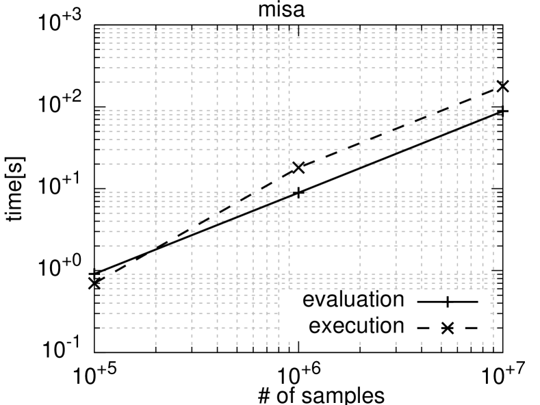
(c)

Figure 1: Motivating example. a) The topology of a GRN with mutual inhibition of genes $A$ and $B$. b) The labelled transition system where labels denote the linear constraints which enable the transition. $\alpha_{0}$, $\alpha_{1}$, $\beta_{0}$, and $\beta_{1}$ denote linear atomic formulas $i_{A}-w_{BA}\leq t_{A}$, $i_{B}+w_{BB}>t_{B}$, $i_{B}-w_{AB}\leq t_{B}$, and $i_{A}+w_{AA}>t_{A}$ respectively. c) Run-times comparison between execution method (dashed lines) and our evaluation method (solid lines).

In the following, we will illustrate the main idea of the paper on an example of a GRN space $T$ generated from the GRN network shown in Fig. 1(a). Two genes $A$ and $B$ inhibit each other, and both genes have a self-activating loop. The parameters $(i_{A},i_{B})$ represent constant inputs, which we assume to be regulated by some other genes that are not presented in the figure. Each of the genes is assigned a threshold value ($t_{A}$, $t_{B}$), and each edge is assigned a weight ($w_{AA}$,$w_{AB}$, $w_{BA}$, $w_{BB}$). The dynamics of a GRN-individual chosen from $T$ depends on these parameters. Genes are in either active or inactive state, which we represent with Boolean variables. For a given initial state of all genes, and for fixed values of weights and thresholds, the values of all genes evolve deterministically in discrete time-steps that are synchronized over all genes. Let $a$ (resp. $b$) be the Boolean variable representing the activity of gene $A$ (resp. $B$). We denote a GRN state by a pair $(a,b)$. Let $\tau$ be the function that governs the dynamics of $\mathcal{G}$ (see Def. 3):

$$\tau(a,b) =(i_{A}+aw_{AA}-bw_{BA}>t_{A},\;i_{B}+bw_{BB}-aw_{AB}>t_{B})$$

The next state of a gene is the result of arithmetically adding the influence from other active genes.

The topology of mutually inhibiting pair of genes is known to be bistable: whenever one gene is highly expressed and the other is barely expressed, the system remains stable [14, 19]. The bistability property can be written as the following LTL formula (see Def. 4):

$$(A\land\neg B\implies\Box(A\land\neg B))\land(\neg A\land B\implies\Box(\neg A\land B)).$$

Let us fix values for parameters $t_{A}=t_{B}=0.6$, $w_{AB}=w_{BA}=w_{BB}=0.3$, and $i_{A}=i_{B}=\frac{2}{3}$. Then, we can check that a GRN is bistable by executing the GRN. Indeed, for the given parameter values, the states $(0,1)$ and $(1,0)$ are fixed points of $\tau$. In other words, the GRN with those parameter values have two stable states: if they start in state $(0,1)$ (resp. $(1,0)$), they remain there. Now let us choose $i_{A}=\frac{2}{3}$, $i_{B}=\frac{1}{3}$. Again, by executing the GRN, we can conclude that it does not satisfy the property: at state $(0,1)$, $B$ does not have sufficiently strong activation to surpass its threshold and the system jumps to $(0,0)$. Intuitively, since the external activation of $B$ is too small, the phenotype has changed to a single stable state. In general, it is not hard to inspect that the bistability property will be met by any choice of parameters satisfying the following constraints:

$$\{i_{A}-w_{BA}\leq t_{A},\;i_{A}+w_{AA}>t_{A},\;i_{B}-w_{AB}\leq t_{B},\;i_{B}+w_{BB}>t_{B}\}.$$ (1)

Let’s now suppose that we want to compute the robustness of $T$ in presence of variations on edges due to mutations. Then, for each possible value of parameters, one needs to verify if the respective GRN satisfies the property. Using the constraints (1), one may verify GRNs without executing them.

Our method automatizes this idea to any given GRN topology and any property specified in LTL. We first encode $T$ as a parametrized labelled transition system, partly shown in  Fig. 1(b). Our implementation does not explicitly construct this transition system, nor executes the GRNs (the implementation is described in Section 5.1). Then, we apply symbolic model checking to compute the constraints which represent the space of GRN’s from $T$ that satisfy the bi-stability property.

To illustrate the scalability of our method in comparison with the standard methods, in Fig. 1(c), we compare the performance of computing the mutational robustness with and without precomputing the constraints (referred to as evaluation and execution method respectively). We choose a mutation model such that each parameter takes 13 possible values distributed according to the binomial distribution (see Appendix for more details on the mutation model). We estimate the robustness value by statistical sampling of the possible parameter values. For a small number of samples, our method is slower because we spend extra time in computing the constraints. However, more samples may be necessary for achieving the desired precision. As the number of samples increases, our method becomes faster, because each evaluation of the constraints is two times faster than checking bistability by executing GRN-individuals. For $1.2\times 10^{5}$ many simulations, execution and evaluation methods take same total time, and the robustness value estimated from these many samples lies in the interval $(0.8871,0.8907)$ with $95\%$ confidence. Hence, for this GRN, if one needs better precision for the robustness value, our method is preferred.

One may think that for this example, we may compute exact robustness because the number of parameter values is only $13^{6}$ (four weights and two inputs). For simplicity of illustration, we chose this example, and we later present examples with a much larger space of parameters, for which exact computation of robustness is infeasible.

2 Preliminaries

In this section, we start by defining a GRN space, which will serve to specify common features for GRNs from the same population. These common features are types of gene interactions (topology), constant parameters (thresholds), and ranges of parameter values that are subject to some environmental perturbation (weights). Then, we formally introduce a model of an individual GRN from the GRN space and temporal logic to express its properties.

2.1 Basic notation

$\mathbb{R}_{\geq 0}$ (resp. $\mathbb{Q}_{\geq 0}$) is the set of non-negative real (resp. rational) numbers. For $m<n$, let $m..n$ denote the set of integers from $m$ to $n$. With abuse of notation, we treat finite maps with ordered domain as vectors with size of the map.

Let $V$ be an infinite set of variable names. For rationals $k_{1},\dots,k_{n}$, a rational variable vector $v=(v_{1},\dots,v_{n})$, and a rational $t$, let $k_{1}v_{1}+\dots+k_{n}v_{n}+t$ denote a linear term. Let $k_{1}v_{1}+\dots+k_{n}v_{n}+t>0$ and $k_{1}v_{1}+\dots+k_{n}v_{n}+t\geq 0$ be a strict and non-strict inequality over $v$ respectively. Let $linear(v)$ be the set of all the (non-)strict inequalities over $v$. Let $polyhedra(v)$ be the set of all the finite conjunctions of the elements of $linear(v)$.

2.2 GRN space

The key characteristics of the behaviour of a GRN are typically summarised by a directed graph where nodes represent genes and edges denote the type of regulation between the genes. A regulation edge is either activation (one gene’s activity increases the activity of the other gene) or repression (one gene’s activity decreases the activity of the other gene) [20]. In Wagner’s model of a GRN, in addition to the activation types between genes, each gene is assigned a threshold and each edge (pair of genes) is assigned a weight. The threshold of a gene models the amount of activation level necessary to sustain activity of the gene. The weight on an edge quantifies the influence of the source gene on destination gene of the edge.

We extend the Wagner’s model by allowing a range of values for weight parameters. We call our model GRN space, denoting that all GRNs instantiated from that space share the same topology, and their parameters fall into given ranges. We assume that each gene always has some minimum level of expression without any external influence. In the model, this constant input is incorporated by a special gene which is always active, and activates all other genes from the network. The weight on the edge between the special gene and some other gene represents the minimum level of activation. The minimal activation is also subject to perturbation.

Definition 1 (GRN space)

A GRN space is a tuple

$$T=(G,g_{in},\leavevmode\hbox to10.01pt{\vbox to3.2pt{\text{[drawing]}}},\leavevmode\hbox to9.01pt{\vbox to5.2pt{\text{[drawing]}}},t,w^{max},{W}),$$

where

• $G=\{g_{1},\ldots,g_{d}\}$ is a finite ordered set of genes,

• $g_{in}\in G$ is the special gene used to model the constant input for all genes,

• $\leavevmode\hbox to9.01pt{\vbox to0.4pt{\text{[drawing]}}}\subseteq G\times G$ is the activation relation such that $\forall g\in G\setminus\{g_{in}\}\;(g_{in},g)\in\leavevmode\hbox to9.01pt{\vbox to0.4pt{\text{[drawing]}}}$ and $\forall g\;(g,g_{in})\notin\leavevmode\hbox to9.01pt{\vbox to0.4pt{\text{[drawing]}}}$,

• $\leavevmode\hbox to9.01pt{\vbox to0.4pt{\text{[drawing]}}}\subseteq G\times G$ is the repression relation such that $\leavevmode\hbox to9.01pt{\vbox to0.4pt{\text{[drawing]}}}\cap\leavevmode\hbox to9.01pt{\vbox to0.4pt{\text{[drawing]}}}=\emptyset\land\forall g\;(g,g_{in})\notin\leavevmode\hbox to9.01pt{\vbox to0.4pt{\text{[drawing]}}}$,

• $t\colon G\to\mathbb{Q}$ is the threshold function such that $\forall g\in G\setminus\{g_{in}\}\;t(g)\geq 0$ and $t(g_{in})<0$,

• $w^{max}\colon(\leavevmode\hbox to9.01pt{\vbox to0.4pt{\text{[drawing]}}}\cup\leavevmode\hbox to9.01pt{\vbox to0.4pt{\text{[drawing]}}})\to\mathbb{Q}_{\geq 0}$ is the maximum value of an activation/repression,

• ${W}=\mathcal{P}((\leavevmode\hbox to9.01pt{\vbox to0.4pt{\text{[drawing]}}}\cup\leavevmode\hbox to9.01pt{\vbox to0.4pt{\text{[drawing]}}})\to\mathbb{Q}_{\geq 0})$ assigns a set of possible weight functions to each activation/inhibition relation, so that $w\in{W}\Rightarrow\forall(g,g^{\prime})\in\leavevmode\hbox to9.01pt{\vbox to0.4pt{\text{[drawing]}}}\cup\leavevmode\hbox to9.01pt{\vbox to0.4pt{\text{[drawing]}}}\;w(g,g^{\prime})\leq w^{max}(g,g^{\prime})$.

In the following text, if not explicitly specified otherwise, we will be referring to the GRN space  $T=(G,g_{in},\leavevmode\hbox to9.01pt{\vbox to0.4pt{\text{[drawing]}}},\leavevmode\hbox to9.01pt{\vbox to0.4pt{\text{[drawing]}}},t,w^{max},{W})$.

2.3 GRN-individual

Definition 2 (GRN-individual)

A GRN-individual $\mathcal{G}$ is a pair $(T,w)$, where $w\in{W}$ is a weight function from the GRN space.

A state $\mathbf{\sigma}\colon G\to\mathbb{B}$ of a GRN-individual $\mathcal{G}=(T,w)$ denotes the activation state of each gene in terms of a Boolean value. Let $\Sigma(\mathcal{G})$ (resp. $\Sigma(T)$) denote the set of all states of $\mathcal{G}$ (resp. $T$), such that $\mathbf{\sigma}(g_{in})=true$. The GRN model executes in discrete time steps by updating all the activation states synchronously and deterministically according to the following rule: a gene is active at next time if and only if the total influence on that gene, from genes active at current time, surpasses its threshold.

Definition 3 (Semantics of a GRN-individual)

A run of a GRN-individual  $\mathcal{G}=(T,w)$ is an infinite sequence of states $\mathbf{\sigma}_{0},\mathbf{\sigma}_{1},\dots$ such that $\mathbf{\sigma}_{n}\in\Sigma(\mathcal{G})$ and $\tau(\mathbf{\sigma}_{n})=\mathbf{\sigma}_{n+1}$ for all $n\geq 0$, where $\tau\colon\Sigma(\mathcal{G})\to\Sigma(\mathcal{G})$ is a deterministic transition function defined by

$$\tau(\mathbf{\sigma}):=\lambda g^{\prime}.\left[\qquad\sum_{\mathrlap{\{g\mid\mathbf{\sigma}(g)\land(g,g^{\prime})\in\leavevmode\hbox to6.43pt{\vbox to0.4pt{\text{[drawing]}}}\}}}w(g)\quad~{}-\quad\sum_{\mathrlap{\{g\mid\mathbf{\sigma}(g)\land(g,g^{\prime})\in\leavevmode\hbox to6.43pt{\vbox to0.4pt{\text{[drawing]}}}\}}}w(g)\qquad>t(g^{\prime})\right]\text{.}$$ (2)

The language of $\mathcal{G}$, denoted by $\llbracket\mathcal{G}\rrbracket$, is a set of all possible runs of $\mathcal{G}$. Note that a GRN-individual does not specify the initial state. Therefore, $\llbracket\mathcal{G}\rrbracket$ may contain more than one run.

2.4 Temporal properties

A GRN exists in a living organism to exhibit certain behaviors. Here we present a linear temporal logic (LTL) to express the expected behaviors of GRNs.

Definition 4 (Syntax of Linear Temporal properties)

The grammar of the language of temporal linear logic formulae are given by the following rules

$$\varphi ::=~{}~{}g~{}\mid~{}(\lnot\varphi)~{}\mid~{}(\varphi\lor\varphi)~{}\mid~{}(\varphi\mathcal{U}\varphi)\text{,}$$

where $g\in G$ is a gene.

Linear temporal properties are evaluated over all (in)finite runs of states from $\Sigma(G)$. Let us consider a run $r=\mathbf{\sigma}_{1},\mathbf{\sigma}_{2},\mathbf{\sigma}_{3},\dots\in\Sigma(G)^{*}\cup\Sigma(G)^{\infty}$. Let $r^{i}$ be the suffix of $r$ after $i$ states and $r_{i}$ is the $i$th state of $r$. The satisfaction relation $\models$ between a run and an LTL formula is defined as follows:

$$r\models g\text{ if }r_{1}(g),\qquad\;\;\;\;r\models\lnot\varphi\text{ if }r\not\models\varphi,\qquad r\models\varphi_{1}\lor\varphi_{2}\text{ if }r\models\varphi_{1}\text{ or }r\models\varphi_{2},$$

$$r\models(\varphi_{1}\mathcal{U}\varphi_{2})\text{ if }\exists i.r^{i}\models\varphi_{2}\text{ and }\forall j\leq i.r^{j}\models\varphi_{1}.$$

Note that if $|r|<i$ then $r^{i}$ has no meaning. In such a situation, the above semantics returns undefined, i.e., $r$ is too short to decide the LTL formula. We say a language ${\cal L}\models\varphi$ if for each run $r\in{\cal L}$, $r\models\varphi$, and a GRN $\mathcal{G}\models\varphi$ if ${\cal L}\llbracket\mathcal{G}\rrbracket\models\varphi$. Let $\Diamond\varphi$ be shorthand of $true\mathcal{U}\varphi$ and $\Box\varphi$ be shorthand of $\lnot\Diamond\lnot\varphi$.

Note that we did not include next operator in the definition of LTL. This is because a typical GRN does not expect something is to be done in strictly next cycle.

3 Algorithm for parameter synthesis

In this section we present an algorithm for synthesizing the weights’ space corresponding to a given property in linear temporal logic. The method combines LTL model checking [2] and satisfiability modulo theory (SMT) solving [4].

The method operates in two steps. First, we represent any GRN-individual  from the GRN space  with a parametrized transition system. In this system, a transition exists between every two states, and it is labelled by linear constraints, that are necessary and sufficient constraints to enable that transition in a concrete GRN-individual  (for example, see Fig. 1b)). We say that a run of the parametrized transition system is feasible if the conjunction of all the constraints labelled along the run is satisfiable. Second, we search for all the feasible runs that satisfy the desired LTL property and we record the constraints collected along them. The disjunction of such run constraints fully characterizes the regions of weights which ensure that LTL property holds in the respective GRN-individual.

Definition 5 (Parametrized transition system)

For a given GRN space  $T$ and rational parameters map $v:G\to V$, the parametrized transition system $(T,v)$ is a labelled transition system $(\Sigma(T),\Phi)$, where the labeling of edges $\Phi:\Sigma(T)\times\Sigma(T)\to polyhedra(v)$ is defined as follows:

$$\Phi:=\lambda\mathbf{\sigma}\mathbf{\sigma}^{\prime}.\bigwedge_{g^{\prime}\in G}\left[\quad\sum_{\mathrlap{\{g\mid\mathbf{\sigma}(g)\land(g,g^{\prime})\in\leavevmode\hbox to6.43pt{\vbox to0.4pt{\text{[drawing]}}}\}}}v(g)\quad~{}-\quad\sum_{\mathrlap{\{g\mid\mathbf{\sigma}(g)\land(g,g^{\prime})\in\leavevmode\hbox to6.43pt{\vbox to0.4pt{\text{[drawing]}}}\}}}v(g)\;\;>\;\;t(g^{\prime})\iff\mathbf{\sigma}^{\prime}(g^{\prime})\right]\text{.}$$

$\Phi(\mathbf{\sigma},\mathbf{\sigma}^{\prime})$ says that a gene $g^{\prime}$ is active in $\mathbf{\sigma}^{\prime}$ iff the weighted sum of activation and suppression activity of the regulators of $g^{\prime}$ is above its threshold.

A run of $(T,v)$ is a sequence of states $\mathbf{\sigma}_{0},\mathbf{\sigma}_{1},\dots$ such that $\mathbf{\sigma}_{n}\in\Sigma(T)$ for all $n\geq 0$, and $\Phi(\mathbf{\sigma}_{0},\mathbf{\sigma}_{1})\land\Phi(\mathbf{\sigma}_{1},\mathbf{\sigma}_{2})\land\dots$ is said to be the run constraint of the run. A run is feasible if its run constraint is satisfiable. We denote by $\llbracket(T,v)\rrbracket$ the set of feasible traces for $(T,v)$. For a weight function ${w}$, let $\Phi(\mathbf{\sigma},\mathbf{\sigma}^{\prime})[{w}/v]$ denote the formula obtained by substituting $v$ by ${w}$ and let $(T,v)[{w}/v]=(\Sigma(T),\Phi^{\prime})$, where $\Phi^{\prime}(\mathbf{\sigma},\mathbf{\sigma}^{\prime})=\Phi(\mathbf{\sigma},\mathbf{\sigma}^{\prime})[{w}/v]$ for each $\mathbf{\sigma},\mathbf{\sigma}^{\prime}\in\Sigma(T)$.

In the following text, we refer to the parametrized transition system $(T,v)$ and an LTL property $\varphi$. Moreover, we denote the run constraint of run $r=\mathbf{\sigma}_{0},\mathbf{\sigma}_{1},\ldots\in\llbracket(T,v)\rrbracket$ by ${cons}(r)$.

Lemma 1

For a weight function ${w}$, the set of feasible runs of $(T,v)[{w}/v]$ is equal to $\llbracket(T,{w})\rrbracket$.

The proof of the above lemma follows from the definition of the semantics for GRN-individual. Note that the run constraints are conjunctions of linear (non)-strict inequalities. Therefore, we may apply efficient SMT solvers to analyze $(T,v)$.

3.1 Constraint generation via model checking

1
2
3
4
5




6
7
8
9
10
11
12
13
14
15

function $\textsc{GenCons}((T,v)=(\Sigma(T),\Phi),\varphi)$

begin

$goodCons:=true$

for each $\mathbf{\sigma}\in\Sigma(T)$ do

$goodCons:=\textsc{GenConsRec}(\mathbf{\sigma},true,goodCons,\Sigma(T),\Phi,\varphi)$

done

return $goodCons$

end

function $\textsc{GenConsRec}(run.\mathbf{\sigma},runCons,goodCons,\Sigma(T),\Phi,\varphi)$

begin

if $|run.\mathbf{\sigma}|<|\Sigma(T)|$ then

for each $\mathbf{\sigma}^{\prime}\in\Sigma(T)$ do

$runCons^{\prime}:=runCons\land\Phi(\mathbf{\sigma},\mathbf{\sigma}^{\prime})$

if $goodCons\wedge runCons^{\prime}$ is sat then

if $run.\mathbf{\sigma}\mathbf{\sigma}^{\prime}\models\neg\varphi$ then $(\ast$ check may return undef $\ast)$

$goodCons:=goodCons\land\neg runCons^{\prime}$

else

$goodCons:=\textsc{GenConsRec}(run.\mathbf{\sigma}\mathbf{\sigma}^{\prime},runCons^{\prime},goodCons,\Sigma(T),\Phi,\varphi)$

   done

return $goodCons$

end

Figure 2: Counterexample guided computation of the mutation space feasible wrt. $\varphi$. Let “.” be an operator that appends two sequences. $run.\mathbf{\sigma}\mathbf{\sigma}^{\prime}\models\neg\varphi$ can be implemented by converting $\neg\varphi$ into a Büchi automaton and searching for an accepting run over $run.\mathbf{\sigma}\mathbf{\sigma}^{\prime}$. However, a finite path may be too short to decide whether $\varphi$ holds or not. In that case, the condition at line 10 fails. Since $(T,v)$ is finite, the finite runs are bound to form lassos within $|\Sigma(T)|$ steps. If a finite run forms a lasso, then the truth value of $run.\mathbf{\sigma}\mathbf{\sigma}^{\prime}\models\neg\varphi$ will be determined.

Now our goal is to synthesize the constraints over $v$ which characterise exactly the set of weight functions $w$, for which $(T,{w})$ satisfies $\varphi$. Each feasible run violating $\varphi$ reports a set of constraints which weight parameters should avoid. Once all runs violating $\varphi$ are accounted for, the desired region of weights is completely characterized. More explicitly, the desired space of weights is obtained by conjuncting negations of run constraints of all feasible runs that satisfy $\neg\varphi$.

In Fig. 2, we present our algorithm GenCons for the constraint generation. GenCons unfolds $(T,v)$ in depth-first-order manner to search for runs which satisfy $\neg\varphi$. At line 3, GenCons calls recursive function GenConsRec to do the unfolding for each state in $\Sigma(T)$. GenConsRec takes six input parameters. The parameter $run.\mathbf{\sigma}$ and $runCons$ are the states of the currently traced run and its respective run constraint. The third parameter are the constraints, collected due to the discovery of counterexamples, i.e., runs which violate $\varphi$. The forth, fifth and sixth parameter are the description of the input transition system and the LTL property $\varphi$. Since GRN-individuals have deterministic transitions, we only need to look for the lassos upto length $|\Sigma(T)|$ for LTL model checking. Therefore, we execute the loop at line 7 only if the $run.\mathbf{\sigma}$ has length smaller than $|\Sigma(T)|$. The loop iterates over each state in $\Sigma(T)$. The condition at line 9 checks if $run.\mathbf{\sigma}\mathbf{\sigma}^{\prime}$ is feasible and, if it is not, the loop goes to another iteration. Otherwise, the condition at line 10 checks if $run.\mathbf{\sigma}\mathbf{\sigma}^{\prime}\models\neg\varphi$. Note that $run.\mathbf{\sigma}\mathbf{\sigma}^{\prime}\models\neg\varphi$ may also return undefined because the run may be too short to decide the LTL property. If the condition returns true, we add negation of the run constraint in $goodCons$. Otherwise, we make a recursive call to extend the run at line 13. $goodCons$ tells us the set of values of $v$ for which we have discovered no counterexample. GenCons returns $goodCons$ at the end.

Since run constraints are always a conjunction of linear inequalities, $goodCons$ is a conjunction of clauses over linear inequalities. Therefore, we can apply efficient SMT technology to evaluate the condition at line 9. The following theorem states that the algorithm GenCons computes the parameter region which satisfies property $\varphi$.

Theorem 3.1

For every weight function $w\in{W}$, the desired set of weight functions for which a GRN-individual  satisfies $\varphi$ equals the weight functions which satisfy the constraints returned by GenCons:

$$(T,w)\models\varphi\hbox{ iff }w\models\textsc{GenCons}((T,v),\varphi).$$

Proof

The statement amounts to showing that the sets $A=\{w\mid(T,w)\models\varphi\}$ and $B=\bigcap_{r\in\llbracket(T,v)\rrbracket\wedge r\models\neg\varphi}\{w\mid w\models\neg{cons}(r)\}$ are equivalent. Notice that

$$W\setminus A =\{w\mid\exists r\in\llbracket(T,v)\rrbracket\hbox{ such that }w\models cons(r)\wedge r\models\neg\varphi\}$$

$$=\bigcup_{r\in\llbracket(T,v)\rrbracket\wedge r\models\neg\varphi}\{w\mid w\models cons(r)\}$$

$$=W\setminus\bigcap_{r\in\llbracket(T,v)\rrbracket\wedge r\models\neg\varphi}\{w\mid w\models\neg cons(r)\}.$$

We use the above presentation of the algorithm for easy readability. However, our implementation of the above algorithm differs significantly from the presentation. We follow the encoding of [7] to encode the path exploration as a bounded-model checking problem. Further details about implementation are available in Section 5. The algorithm has exponential complexity in the size of $T$. However, one may view the above procedure as the clause learning in SMT solvers, where clauses are learnt when the LTL formula is violated [23]. Similar to SMT solvers, in practice, this algorithm may not suffer from the worst-case complexity.

Example 1

The GRN osc3 (shown in  Fig. 3) was the model of a pioneering work in synthetic biology [12], and it is known to provide oscillatory behaviour: each gene should alternate its expression between ‘on’ and ‘off’ state:

$$\varphi_{3}=\bigwedge_{v\in\{A,B,C\}}(v\Rightarrow\Diamond\neg{v})\wedge(\neg{v}\Rightarrow\Diamond{v}).$$

The solutions are the constraints:

$$(T,w)\models\varphi_{3} \hbox{ iff }(i_{A}>t_{A})\wedge(i_{B}>t_{B})\wedge(i_{C}>t_{C})\wedge$$

$$(i_{B}-w_{AB}\leq t_{B})\wedge(i_{C}-w_{BC}\leq t_{C})\wedge(i_{A}-w_{CA}\leq t_{A}).$$

4 Computing Robustness

In this section, we present an application of our parameter synthesis algorithm, namely computing robustness of GRNs in presence of mutations. To this end, we formalize GRN-population and its robustness. Then, we present a method to compute the robustness using our synthesized parameters.

A GRN-population  models a large number of GRN-individuals with varying weights. All the GRN-individuals are defined over the same GRN space, hence they differ only in their weight functions. The GRN-population  is characterised by the GRN space  $T$ and a probability distribution over the weight functions. In the experimental section, we will use the range of weights ${W}$ and the distribution $\pi$ based on the mutation model outlined in the Appendix.

Definition 6 (GRN-population)

A GRN-population  $\mathcal{Z}$ is a pair $(T,\pi)$, where $\pi:{W}\rightarrow[0,1]$ is a probability distribution over all weight functions from GRN space $T$.

We write $\varphi({\mathcal{Z}})\in[0,1]$ to denote an expectation that a GRN instantiated from a GRN-population $\mathcal{Z}=(T,\pi)$ satisfies $\varphi$. The value $\varphi({\mathcal{Z}})$ is in the interval $[0,1]$ and we call it robustness.

Definition 7 (Robustness)

Let $\mathcal{Z}=(T,\pi)$ be a GRN-population, and $\varphi$ be an LTL formula which expresses the desired LTL property. Then, robustness of $\mathcal{Z}$ with respect to property $\varphi$ is given by

$$\varphi(\mathcal{Z}):=\sum_{\{w\mid\llbracket(T,w)\rrbracket\models\varphi\}}\pi(w)$$

The above definition extends that of [10], because it allows for expressing any LTL property as a phenotype, and hence it can capture more complex properties such as oscillatory behaviour.

In the following, we will present an algorithm for computing the robustness, which employs algorithm GenCons.

4.1 Evaluating robustness

Let us suppose we get a GRN-population  $\mathcal{Z}=(T,\pi)$ and LTL property $\varphi$ as input to compute robustness.

For small size of GRN space $T$, robustness can be computed by explicitly enumerating all the GRN-individuals from $T$, and verifying each GRN-individual  against $\varphi$. The probabilities of all satisfying GRN-individuals are added up. However, the exhaustive enumeration of the GRN space  is often intractable due to a large range of weight functions ${W}$ in $T$. In those cases, the robustness is estimated statistically: a number of GRN-individuals are sampled from $T$ according to the distribution $\pi$, and the fraction of satisfying GRN-individuals is stored. The sampling experiment is repeated a number of times, and the mean (respectively variance) of the stored values are reported as robustness (respectively precision).

Depending on how a sampled GRN-individual is verified against the LTL property, we have two methods:

• In the first method, which we will call execution method, each sampled GRN-individual is verified by executing the GRN-individual  from all initial states and checking if each run satisfies $\varphi$;

• In the second method, which we will call evaluation method, the constraints are first precomputed with GenCons, and each sampled GRN-individual  is verified by evaluating the constraints.

Clearly, the time of computing the constraints initially renders the evaluation method less efficient. This cost is amortized when verifying a GRN-individual by constraint evaluation is faster than by execution. In the experimental section, we compare the overall performance of the two approaches on a number of GRNs from literature.

5 Experimental results

		Property	Space size
mi:		$(Y\bar{Z}\implies\Box Y\bar{Z})\land(Z\bar{Y}\implies\Box Z\bar{Y})$	$4225$
misa:		$(Y\bar{Z}\implies\Box Y\bar{Z})\land(Z\bar{Y}\implies\Box Z\bar{Y})$	$105625$
qi:		$(YS\bar{Z}\bar{R}\implies\Box YS\bar{Z}\bar{R})\hskip 4.0pt\land$ $(\bar{Y}\bar{S}ZR\implies\Box\bar{Y}\bar{S}ZR)$	$\approx 10^{9}$
cc:		$\Diamond\Box X\lor\Diamond\Box\bar{X}$	$\approx 10^{10}$
ncc:		$(YQS\bar{Z}\bar{P}\bar{R}\implies\Box YQS\bar{Z}\bar{P}\bar{R})\hskip 4.0pt\land$ $(\bar{Y}\bar{Q}\bar{S}ZPR\implies\Box\bar{Y}\bar{Q}\bar{S}ZPR)$	$\approx 10^{18}$
oscN:		$X_{1}\implies\Diamond\bar{X_{1}}\land\bar{X_{1}}\implies\Diamond X_{1}\hskip 8.0pt\land$ $X_{2}\implies\Diamond\bar{X_{2}}\land\bar{X_{2}}\implies\Diamond X_{2}\hskip 8.0pt\land$ … $X_{N}\implies\Diamond\bar{X}_{N}\land\bar{X}_{N}\implies\Diamond X_{N}$	3:$274625$ 5:$\approx 10^{9}$ 7:$\approx 10^{12}$

Figure 3: GRN benchmarks. mi, misa (mutual inhibition), qi (quad inhibition), and ncc (cell cycle switch) satisfy different forms of bistability. For the networks ci (cell cycle switch), the value of gene eventually stabilizes [9]. In osc3, also known as the repressilator [12], the gene values alternate. osc5 and osc7 (not shown) are generalizations of osc3, and also exhibit oscilating behavior.

We implemented a tool which synthesizes the parameter constraints for a given LTL property (explained in Section 3), and the methods for computing the mutational robustness (explained in Section 4.1). We ran our tool on a set of GRNs from literature.

5.1 Implementation

Our implementation does not explicitly construct the parametrised transition system described in Section 3 (Dfn. 5 and Alg. 2). Instead, we encode the bounded model-checking (Alg. 2) as a satisfiability problem, and we use an SMT solver to efficiently find $goodCons$. More concretely, we initially build a formula which encodes the parametrized transition system and it is satisfied if and only if some run of $(T,v)$ satisfies $\neg\varphi$. If the encoding formula is satisfiable, the constraints $cons(r)$ along the run are collected, and $\neg cons(r)$ is added to $goodCons$. Then, we expand the encoding formula by adding $\neg cons(r)$, so as to rule out finding the same run again. We continue the search until no satisfying assignment of the encoding formula can be found. The algorithm always terminates because the validity of the property is always decided on finite runs (as explained in Section 3).

The implementation involves 8k lines of C++ and we use Z3 SMT solver as the solving engine. We use CUDD to reduce the size of the Boolean structure of the resulting formula. We ran the experiments on a GridEngine managed cluster system. Our tool, as well as the examples and the simulation results are available online..

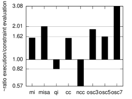
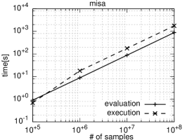
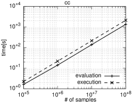
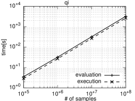
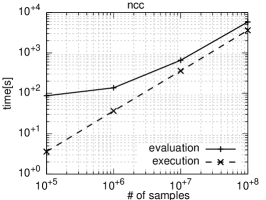
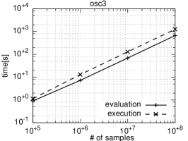
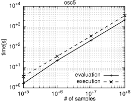
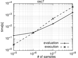
Figure 4: The comparison in performance when mutational robustness is statistically estimated, and a property check is performed either by evaluation, or by execution (see Section 4.1 for the description of the two methods). The bar (top-left) shows the ratio of average times needed to verify the property of one sampled GRN-individual. For example, for osc7, the performance of evaluation method is more than three times faster. The other graphs show how the robustness computation time depends on the total number of sampled GRNs (in order to obtain robustness and to estimate the precision, we computed the mean of $100$ experiments, each containing a number of samples ranging from $10^{3}$ to $10^{6}$). The graph is shown in log-log scale. The non-linear slope of the evaluation method is most notable in examples mcc and osc7, and it is due to the longer time used for compute the constraints.

5.2 Performance evaluation

We chose eight GRN topologies as benchmarks for our tool. The benchmarks are presented in Fig. 3. The first five of the GRN topologies are collected from [8]. On these benchmarks we check for the steady-state properties. On the final three GRN topologies, we check for the oscillatory behavior. The results are presented in Fig. 4.

We ran the robustness computation by the evaluation and execution methods (the methods are described in Section 4.1). In order to obtain robustness and to estimate the precision, we computed the mean of $100$ experiments, each containing a number of samples ranging from $10^{3}$ to $10^{6}$. The total computation time in the execution methods linearly depends on the number of samples used. The total computation time in the evaluation method depends linearly on the number of samples, but initially needs time to compute the constraints. Technically, the time needed to compute robustness by execution method is $t_{ex}=k_{ex}p$, and the time needed to compute robustness by evaluation approach $t_{ev}=k_{ev}p+t_{c}$, where $p$ represents the total number of samples used, $t_{c}$ is the time to compute the constraints, and $k_{ex}$ (resp. $k_{ev}$) is the time needed to verify the property by evaluation (resp. execution). We used linear regression to estimate the parameters $k_{ex}$ and $k_{ev}$, and we present the ratio $\frac{k_{ex}}{k_{ev}}$ in top-left position of Fig. 4. The results indicate that on six out of eight tested networks, evaluation is more efficient than execution. For some networks, such as osc7, the time for computing the constraints is large, and the gain in performance becomes visible only once the number of samples is larger than $10^{6}$.

6 Conclusion and discussion

In this paper, we pursued formal analysis of Wagner’s GRN model, which allows symbolic reasoning about the behavior of GRNs under parameter perturbations. More precisely, for a given space of GRNs and a property specified in LTL, we have synthesized the space of parameters for which the concrete, individual GRN from a given space satisfies the property. The resulting space of parameters is represented by complex linear inequalities. In our analysis, we have encoded a bounded model-checking search into a satisfiability problem, and we used efficient SMT solvers to find the desired constraints. We demonstrated that these constraints can be used to efficiently compute the mutational robustness of populations of GRNs. Our results have shown the cases in which the computation can be three times faster than the standard (simulation) techniques employed in computational biology.

While computing mutational robustness is one of the applications of our synthesized constraints, the constraints allow to efficiently answer many other questions that are very difficult or impossible to answer by executing the sampled GRNs. In our future work, we aim to work on further applications of our method, such as parameter sensitivity analysis for Wagner’s model. Moreover, we plan to work on the method for exact computation of robustness by applying the point counting algorithm [5].

The Wagner’s model of GRN is maybe the simplest dynamical model of a GRN – there are many ways to add expressiveness to it: for example, by incorporating multi-state expression level of genes, non-determinism, asynchronous updates, stochasticity. We are planning to study these variations and chart the territory of applicability of our method.

Mutation model

In this section, we present the mutation model that is grounded in evolutionary biology research. Genetic mutations refer to events of changing base pairs in the DNA sequence of the genes and they may disturb the regular functioning of the host cell. Such mutations affect the weight functions and we assume their range to be between a maximum weight and zero.

0..0.1 Modeling mutations in a nucleotide.

The mutations of a single nucleotide follow a discrete-time Markov chain (DTMC), illustrated in Fig. 5a). When the DNA is passed from the mother to the daughter cell, a ‘correct’ nucleotide (in figure it is the $\mathtt{A}$) can mutate to each different value ($\mathtt{T}$, $\mathtt{C}$ or $\mathtt{G}$) with some probability. In the model in Fig. 5a), the probability of each possible mutation is $\frac{p}{3}$, and hence, the probability of retaining the same nucleotide is $1-p$. In Fig. 5b), there is a process where all mutated states are lumped together - the probability to get to the ‘correct’ nucleotide is equal to $\frac{p}{3}$, and to remain mutated is therefore $(1-\frac{p}{3})$. We will refer to the general probabilities of the lumped process with a matrix

$$P^{id}=\left[\begin{array}[]{ccc}p_{00}&p_{01}\\ p_{10}&p_{11}\end{array}\right],$$

with the intuition $0$ being the non-mutated state and $1$ the mutated state. Let $X_{n}^{i}\in\{\mathbf{0},\mathbf{1}\}$ be a process (DTMC) reporting whether the $i$-th nucleotide is in its ‘correct’ configuration, or mutated configuration at $n$-th generation. The number $P(X_{n}^{i}=\mathbf{1})$ can be interpreted also as that the fraction of mutated $i$-th nucleotides observed in the population at generation $n$. Notably, for the values shown in Fig. 5b), the stationary distribution of $X_{n}^{i}$ is $(0.75,0.25)$, independently of the probability of a single mutation $p$.

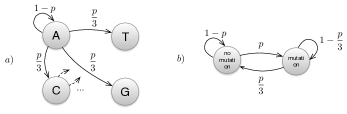
Figure 5: A model of changes of a single nucleotide from one generation to another

0..0.2 Modeling mutations in a single gene.

Let us assume $l$ to be the length of the DNA binding region of a gene $g$, and $P^{id}$ to be specify the probabilities of single point mutations occurring in it. Moreover, we assume that the maximal weight for influence of gene $g$ to $g^{\prime}$, i.e. $w(g,g^{\prime})$, is achieved for a single sequence of nucleotides, and that the weight will linearly decrease with the number of mutated nucleotides (where ‘mutated’ refers to being different to the sequence achieving the maximal weight). Therefore, if $k$ out of $l$ nucleotides in the promoter region of $g^{\prime}$ that is affected by $g$ are mutated, the weight $w(g,g^{\prime})$ becomes $w^{max}(g,g^{\prime})(1-\frac{k}{l})$.

If the whole promoter sequence of one gene is modelled by a string $\mathbf{a}\in\{\mathtt{A},\mathtt{T},\mathtt{C},\mathtt{G}\}^{l}$, its changes over generations are captured by an $l$-dimensional random process $(X_{n}^{1},\ldots,X_{n}^{l})(\mathbf{a})\in\{\mathbf{0},\mathbf{1}\}^{l}$. Mutation events $X_{n}^{1}$, $X_{n}^{2}$,…, $X_{n}^{l}$ are assumed to happen independently within the genome, and independently of the history of mutations. Then, a random process $M_{n}:=X_{n}^{1}+\ldots+X_{n}^{l}$, such that $M_{n}=k\in\{0,\ldots,l\}$, denotes that the configuration at generation $n$ differs from the optimal configuration in exactly $k$ points. The following lemma defines the values of the transition matrix of the process $\{M_{n}\}$.

Lemma 2

The process $\{M_{n}\}$ is a DTMC, with transition probabilities $P(M_{n+1}=j\mid M_{n}=i)=T({i,j})$, where $T:0..l\times 0..l\to[0,1]$ amounts to:

$$T(i,j):=\sum_{u=0}^{\min\{i,j\}}{i\choose u}p_{11}^{u}p_{10}^{i-u}{{l-i}\choose{j-u}}p_{01}^{j-u}p_{00}^{l-i-(j-u)}.$$ (3)

Moreover, $\{M_{n}\}$ converges to a unique stationary distribution, which is a binomial, with success probability $\beta=\lim_{n\to\infty}P(X_{n}^{i}=\mathbf{1})$. In a special case $\hat{P}^{id}=\left[\begin{array}[]{ccc}1-p&{p}\\ \frac{p}{3}&1-\frac{p}{3}\end{array}\right]$, the stationary distribution is $\beta=\frac{3}{4}$, independently of the value of $p$.

Proof

(Lem. 2) It suffices to observe that $u$ represents the number of mutated nucleotides which remain mutated at time $(n+1)$, and $(j-u)$ is the number of unmated nucleotides which become mutated at time $(n+1)$. The existence and convergence of the stationary trivially follows from that $\{M_{n}\}$ is regular (irreducible and aperiodic). Each process $\{X_{n}^{i}\}$ at a stationary behaves as a Bernoulli process, with probability of being mutated equal to $\beta=\lim_{n\to\infty}P(X_{n}^{i}=1)$, and a probability of remaining un-mutated $1-\beta$. The claim follows as the sum of $l$ independent Bernoulli processes is binomially distributed. The special case follows because matrix $\hat{P}^{id}$ has a unique stationary distribution $(0.25,0.75)$ (denoting by $a$ and $b$ its coordinates, we obtain equations $a(1-p)+b\frac{p}{3}=a$ and $ap+b(1-\frac{p}{3})=b$, which can be satisfied only if $a=\frac{b}{3}$).

Remark that in a special case when $p_{00}=0.25$, the transition matrix of the process $\{M_{t}\}$ has the transition probabilities

$$P(K_{n+1}=j\mid K_{n}=i) =p_{11}^{j}p_{00}^{l-j}\sum_{u=0}^{i}{i\choose u}{{l-i}\choose{j-u}}$$

$$={l\choose j}0.75^{j}0.25^{l-j},$$

which do not depend on $i$.

The special case of matrix $T$ for $l=2$ is illustrated in Fig. 6.

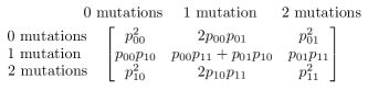
Figure 6: The transition matrix for the evolutionary process of one gene with two nucleotides. The transition probabilities are computed based on the assumption that the single nucleotide mutations happen independently across the genome: for example, the transition from zero to two mutation is equal to $p_{01}^{2}$, because it occurs iff both nucleotides transition from a correct to a mutated state.

0..0.3 Modeling mutations in a GRN.

We assume that mutations happen independently across the genome, and therefore, if the genome is in the configuration $\mathbf{k}=(k_{1},\ldots,k_{d})$, the probability that the next generation will be in the configuration $\mathbf{k}^{\prime}=(k_{1}^{\prime},\ldots,k_{d}^{\prime})$ will be a product of transition probabilities from $k_{i}$ to $k_{i}^{\prime}$, for $i=1,\ldots,d$.

Each sequence $\mathbf{k}=(k_{1},\ldots,k_{d})\in 0..l_{1}\times\ldots\times 0..l_{d}$ defines one weight function $w_{\mathbf{k}}$, with $w_{\mathbf{k}}(g_{i},g_{j})=w^{max}(g_{i},g_{j})(1-\frac{k_{j}}{l_{j}})$. Hence, the domain of weight functions is given by

$${W}=\{w_{\textbf{k}}\mid\textbf{k}\in 0..l_{1}\times\ldots\times 0..l_{d}\},$$

and the distribution is given by

$$\pi(w_{\textbf{k}})=\prod_{i=1}^{d}{d\choose k_{i}}\beta^{k_{i}}(1-\beta)^{d-k_{i}}.$$

References

- [1] R. B. R. Azevedo, R. Lohaus, S. Srinivasan, K. K. Dang, and C. L. Burch. Sexual reproduction selects for robustness and negative epistasis in artificial gene networks. Nature, 440(7080):87–90, Mar. 2006.
- [2] C. Baier and J.-P. Katoen. Principles of model checking. MIT Press, 2008.
- [3] C. Barrett, M. Deters, L. de Moura, A. Oliveras, and A. Stump. 6 years of SMT-COMP. Journal of Automated Reasoning, 50(3):243–277, 2013.
- [4] C. W. Barrett, R. Sebastiani, S. A. Seshia, and C. Tinelli. Satisfiability modulo theories. Handbook of satisfiability, 185:825–885, 2009.
- [5] A. Barvinok and J. E. Pommersheim. An algorithmic theory of lattice points in polyhedra. New perspectives in algebraic combinatorics, 38:91–147, 1999.
- [6] G. Batt, C. Belta, and R. Weiss. Model checking genetic regulatory networks with parameter uncertainty. In Hybrid systems: computation and control, pages 61–75. Springer, 2007.
- [7] A. Biere, A. Cimatti, E. M. Clarke, O. Strichman, and Y. Zhu. Bounded model checking. Advances in computers, 58:117–148, 2003.
- [8] L. Cardelli. Morphisms of reaction networks that couple structure to function.
- [9] L. Cardelli and A. Csikász-Nagy. The cell cycle switch computes approximate majority. Scientific reports, 2, 2012.
- [10] S. Ciliberti, O. C. Martin, and A. Wagner. Robustness can evolve gradually in complex regulatory gene networks with varying topology. PLoS Computational Biology, 3(2), 2007.
- [11] V. Danos and C. Laneve. Formal molecular biology. Theoretical Computer Science, 325(1):69–110, 2004.
- [12] M. B. Elowitz and S. Leibler. A synthetic oscillatory network of transcriptional regulators. Nature, 403(6767):335–338, 2000.
- [13] J. Fisher and T. A. Henzinger. Executable cell biology. Nature biotechnology, 25(11):1239–1249, 2007.
- [14] T. S. Gardner, C. R. Cantor, and J. J. Collins. Construction of a genetic toggle switch in escherichia coli. Nature, 403(6767):339–342, 2000.
- [15] S. K. Jha, E. M. Clarke, C. J. Langmead, A. Legay, A. Platzer, and P. Zuliani. A bayesian approach to model checking biological systems. In Computational Methods in Systems Biology, pages 218–234. Springer, 2009.
- [16] M. Kwiatkowska, G. Norman, and D. Parker. Using probabilistic model checking in systems biology. ACM SIGMETRICS Performance Evaluation Review, 35(4):14–21, 2008.
- [17] T. MacCarthy, R. Seymour, and A. Pomiankowski. The evolutionary potential of the drosophila sex determination gene network. Journal of Theoretical Biology, 225(4):461–468, 2003.
- [18] R. Mateescu, P. T. Monteiro, E. Dumas, and H. De Jong. Ctrl: Extension of ctl with regular expressions and fairness operators to verify genetic regulatory networks. Theoretical Computer Science, 412(26):2854–2883, 2011.
- [19] A. Rizk, G. Batt, F. Fages, and S. Soliman. A general computational method for robustness analysis with applications to synthetic gene networks. Bioinformatics, 25(12):i169–i178, 2009.
- [20] T. Schlitt and A. Brazma. Current approaches to gene regulatory network modelling. BMC bioinformatics, 8(Suppl 6):S9, 2007.
- [21] A. Wagner. Does evolutionary plasticity evolve? Evolution, 50(3):1008–1023, 1996.
- [22] B. Yordanov, C. M. Wintersteiger, Y. Hamadi, and H. Kugler. SMT-based analysis of biological computation. In NASA Formal Methods, pages 78–92. Springer, 2013.
- [23] L. Zhang, C. F. Madigan, M. H. Moskewicz, and S. Malik. Efficient conflict driven learning in a boolean satisfiability solver. In Proceedings of the 2001 IEEE/ACM international conference on Computer-aided design, pages 279–285. IEEE Press, 2001.