Achievable Throughput and Training Optimization of Uplink Multiuser Massive MIMO Systems

Abstract

We study the performance of uplink transmission in a large-scale (massive) MIMO system, where all the transmitters have single antennas and the base station has a large number of antennas. Specifically, we first derive the rates that are possible through minimum mean-squared error (MMSE) channel estimation and three linear receivers: maximum ratio combining (MRC), zero-forcing (ZF), and MMSE. Based on the derived rates, we quantify the amount of energy savings that are possible through increased number of base-station antennas or increased coherence interval. We also analyze achievable total degrees of freedom (DoF) of such a system without assuming channel state information at the receiver, which is shown to be the same as that of a point-to-point MIMO channel. Linear receiver is sufficient to achieve total DoF when the number of users is less than the number of antennas. When the number of users is equal to or larger than the number of antennas, nonlinear processing is necessary to achieve the full degrees of freedom. Finally, the training period and optimal training energy allocation under the average and peak power constraints are optimized jointly to maximize the achievable sum rate when either MRC or ZF receiver is adopted at the receiver.

I Introduction

Massive multiple-input multiple-output (MIMO) systems are a type of cellular communication where the base station is equipped with a large number of antennas. The base station serves multiple mobile stations that are usually equipped with a small number of antennas, typically one. Massive MIMO holds good potential for improving future communication system performance. There are several challenges with designing such massive MIMO systems, including e.g., channel state information (CSI) acquisition [24], base station received signal processing [8], downlink precoding with imperfect CSI [20], signal detection algorithm [10], etc. For multi-cell system, pilot contamination and inter-cell interference also need to be dealt with [13]. There is already a body of results in the literature about the analysis and design of large MIMO systems; see e.g., the overview articles [25, 15] and references there in.

To reveal the potential that is possible with massive MIMO systems, it is important to quantify the achievable performance of such systems in realistic scenarios. For example, it is too optimistic to assume that perfect CSI can be acquired at the base station in the uplink, because such acquisition takes time, energy, and channel estimation error will always exist. For the downlink, in order to perform effective beamforming, CSI is again needed, which needs to be either estimated by the mobile stations and then fed back to the base station, which is a non-trivial task, or, acquired by the base station by exploiting channel reciprocity in a time-division duplexing setup.

I-A Scope of this paper

In this paper, we are interested in performance of the uplink transmission in a single-cell system. In particular, we ask what rates can be achieved in the uplink by the mobile users if we assume realistic channel estimation at the base station. Similar analysis has been performed in [22, 28, 29], but the analysis therein assumes equal power transmission during the channel training phase and the data transmission phase. Also, the effect of channel coherence interval on system throughput was discussed in [4] and power allocation and training duration optimization for the uplink MIMO system were considered in [16] for single-cell system and in [23] for a multi-cell system. However, peak power constraint was not considered. For a fixed training period, to obtain an accurate estimate the training power needs to be high to enable enough training energy. As a result, peak power constraint, if present, may be violated. The solution is to optimize the training duration also.

If we allow the users to cooperate, then the system can be viewed as a point-to-point MIMO channel. The rates obtained in [11], and the stronger result on non-coherent MIMO channel capacity in [30] can serve as upper bound for the system sum rate. The question is how much of this sum rate can be achieved without user cooperation and without using elaborate signaling such as signal packing on Grassmannian manifolds.

For a system with $K$ mobile users, $M$ base station antennas, and block fading channel with coherence interval $T$, we derive achievable rate using linear channel estimation and linear base station (front-end) processing, including maximum ratio combining (MRC), zero-forcing (ZF), and minimum mean-squared estimation (MMSE) processing. The total degrees of freedom (DoF) is also quantified. We also quantify the needed transmission power for achieving a given rate, when $M\gg 1$, which is an refinement of the corresponding result in [22].

Furthermore, the energy allocation and training duration are also both optimized for uplink multi-user (MU) MIMO systems in a systematic way. Two linear receivers, MRC and ZF, are adopted with imperfect CSI. The average and peak power constraints are both incorporated. We analyze the convexity of this optimization problem, and derive the optimal solution. The solution is in closed form except in one case where a one-dimensional search of a quasi-concave function is needed. Simulation results are also provided to demonstrate the benefit of optimized training, compared to equal power allocation considered in the literature.

The main contributions of this paper are listed as follows:

1. We consider the energy allocation between training phase and data phase, and derive achievable rate using linear channel estimation and linear base station (front-end) processing, including MRC, ZF and MMSE processing.

2. We quantify the total degrees of freedom (DoF) with estimated channels.

3. We quantify the needed transmission power for achieving a given rate, when $M\gg 1$, which is an refinement of the corresponding result in [22].

4. We provide a complete solution for the optimal training duration and training energy in an uplink MU-MIMO system with both MRC and ZF receiver, under both peak and average power constraints.

I-B Related Works

The throughput of massive MIMO systems has been studied in several recent papers. For example, the issue of non-ideal hardware and its effect on the achievable rates were investigated in [3, 4]. In [22, 21], the achievable rates with perfect or estimated CSI were derived and scaling laws were obtained in terms of the power savings as the number base station antennas is increased. For channel estimation, the training power and training duration were not optimized for rate maximization. Expressions for uplink achievable rates under perfect or imperfect CSI were derived in [29] for Ricean channels with an arbitrary-rank deterministic component. For the downlink MIMO broadcast channel, the optimization over training period and power in both training phase and feedback phase was investigated in [14]. An optimized energy reduction scheme was proposed in [19] for uplink MU MIMO in a single cell scenario, where both RF transmission power and circuit power consumption were incorporated. Wireless energy transfer using massive MIMO was considered in [27], where the uplink channels were estimated and the uplink rate for the worst user was maximized. Downlink throughput scaling behavior was investigated in [2], where it was shown that unused uplink throughput can be used to trade off for downlink throughput and that the downlink throughput is proportional to the logarithm of the number of base-station antennas. Stochastic geometry was used [1] to analyze the uplink SINR and rate performance of large-scale massive MIMO systems with maximum ratio combining or zero-forcing receivers. Scaling laws between the required number of antennas and the number of users to maintain the same signal to interference ratio (SIR) distributions were derived.

The rest of the paper is organized as follows. A system model is developed in Section II. The channel estimation is discussed in Section III. The achievable rates for linear receivers and the achievable total degrees of freedom of the system are derived in Section IV. Section V formulates the problem of maximization of achievable rate with both average and peak power constraints. The solution of this optimization problem is presented in Sections VI and VII. When $M\to\infty$, simplified expressions for the achievable rates are discussed in Section VIII. Numerical simulation results are reported in Section IX and finally conclusions are drawn in Section X.

II System Model

Notation: We use $\mathbf{A}^{\dagger}$ to denote the Hermitian transpose of a matrix $\mathbf{A}$, $\mathbf{I}_{K}$ to denote a $K\times K$ identity matrix, ${\mathbb{C}}$ to denote the complex number set, $\lfloor\cdot\rfloor$ to denote the integer floor operation, i.i.d. to denote “independent and identically distributed”, and $\mathcal{CN}(0,1)$ to denote circularly symmetric complex Gaussian distribution with zero mean and unit variance.

Consider a single-cell uplink system, where there are $K$ mobile users and one base station. Each user is equipped with one transmit antenna, and the base station is equipped with $M$ receive antennas. The received signal at the base station is expressible as

$$\mathbf{y}=\mathbf{H}\mathbf{s}+\mathbf{n}$$ (1)

where $\mathbf{H}\in{\mathbb{C}}^{M\times K}$ is the channel matrix, $\mathbf{s}\in{\mathbb{C}}^{K\times 1}$ is the transmitted signals from all the $K$ users; $\mathbf{n}\in{\mathbb{C}}^{M\times 1}$ is the additive noise, $\mathbf{y}\in{\mathbb{C}}^{M\times 1}$ is the received signal. We make the following assumptions:

A1) The channel is block fading such that within a coherence interval of $T$ channel uses, the channel remains constant. The entries of $\mathbf{H}$ are i.i.d. and taken from ${\mathcal{C}\mathcal{N}}(0,1)$. The channel changes independently from block to block. The CSI is neither available at the transmitters nor at the receiver.

A2) Entries of the noise vector $\mathbf{n}$ are i.i.d. and from ${\mathcal{C}\mathcal{N}}(0,1)$. Noises in different channel uses are independent.

A3) The average transmit power per user per symbol is $\rho$. So within a coherence interval the total transmitted energy is $\rho T$.

In summary, the system has four parameters, $(M,K,T,\rho)$. We will allow the system to operate in the ergodic regime, so coding and decoding can occur over multiple coherent intervals.

III Channel Estimation

We assume that $K\leq M$ and $K<T$ in this section. To derive the achievable rates for the users, we use a well-known scheme that consists of two phases (see e.g., [11]):

Training Phase. This phase consists of $T_{\tau}$ time intervals. The $K$ users send time-orthogonal signals at power level $\rho_{\tau}$ per user. The training signal transmitted can be represented by a $K\times T_{\tau}$ matrix $\mathbf{\Phi}$ such that $\mathbf{\Phi}\mathbf{\Phi}^{\dagger}=E\mathbf{I}_{K}$, where $E=\rho_{\tau}T_{\tau}$ is the total training energy per user per coherent interval. Note that we require $T_{\tau}\geq K$ to satisfy the time-orthogonality.

Data Transmission Phase. Information-bearing symbols are transmitted by the users in the remaining $T_{d}=T-T_{\tau}$ time intervals. The average power per symbol per user is $\rho_{d}=(\rho T-E)/T_{d}$.

III-A MMSE Channel Estimation

In the training phase, we will choose $\mathbf{\Phi}=\sqrt{E}\mathbf{I}_{K}$ for simplicity. Other scaled unitary matrix can also be used without affecting the achievable rate. Note that the transmission power is allowed to vary from the training phase to the data transmission phase. With our choice of $\mathbf{\Phi}$, the received signal $\mathbf{Y}_{p}\in\mathbb{C}^{M\times T_{\tau}}$ during the training phase can be written as

$$\mathbf{Y}_{p}=\mathbf{H}\mathbf{\Phi}+\mathbf{N}=\sqrt{E}\mathbf{H}+\mathbf{N}$$ (2)

where $\mathbf{N}\in\mathbb{C}^{M\times T_{\tau}}$ is the additive noise. The equation describes $M\times T_{\tau}$ independent identities, one for each channel coefficient. The (linear) MMSE estimate for the channel $\mathbf{H}$ is given by

$$\widehat{\mathbf{H}}=\frac{\sqrt{E}}{E+1}\mathbf{Y}_{\text{p}}=\frac{E}{E+1}\mathbf{H}+\frac{\sqrt{E}}{E+1}\mathbf{N}.$$ (3)

The channel estimation error is defined as

$$\widetilde{\mathbf{H}}=\mathbf{H}-\widehat{\mathbf{H}}=\frac{1}{E+1}\mathbf{H}-\frac{\sqrt{E}}{E+1}\mathbf{N}.$$ (4)

It is well known and easy to verify that the elements of $\widehat{\mathbf{H}}$ are i.i.d. complex Gaussian with zero mean and variance

$$\sigma_{\widehat{\mathbf{H}}}^{2}=\frac{E}{E+1},$$ (5)

and the elements of $\widetilde{\mathbf{H}}$ are i.i.d. complex Gaussian with zero mean and variance

$$\sigma_{\widetilde{\mathbf{H}}}^{2}=\frac{1}{E+1}.$$ (6)

Moreover, $\widehat{\mathbf{H}}$ and $\widetilde{\mathbf{H}}$ are in general uncorrelated as a property of linear MMSE estimator, and in this case independent thanks to the Gaussian assumptions.

III-B Equivalent Channel

Once the channel is estimated, the base station has $\widehat{\mathbf{H}}$ and will decode the users’ information using $\widehat{\mathbf{H}}$. We can write the received signal as

$$\mathbf{y}=\widehat{\mathbf{H}}\mathbf{s}+\widetilde{\mathbf{H}}\mathbf{s}+\mathbf{n}:=\widehat{\mathbf{H}}\mathbf{s}+\mathbf{v}$$ (7)

where $\mathbf{v}\operatorname{:\!=}\widetilde{\mathbf{H}}\mathbf{s}+\mathbf{n}$ is the new equivalent noise containing actual noise $\mathbf{n}$ and self interference $\widetilde{\mathbf{H}}\mathbf{s}$ caused by inaccurate channel estimation. Assuming that each element of $\mathbf{s}$ has variance $\rho_{d}$ during the data transmission phase, and there is no cooperation among the users, the variance of each component of $\mathbf{v}$ is

$$\sigma_{v}^{2}=\frac{K\rho_{d}}{E+1}+1.$$ (8)

If we replace $\mathbf{v}$ with a zero-mean complex Gaussian noise with equal variance $\sigma_{v}^{2}$, but independent of $\mathbf{s}$, then the system described in (7) can be viewed as MIMO system with perfect CSI at the receiver, and equivalent signal to noise ratio (SNR)

$$\rho_{\text{eff}}\operatorname{:\!=}\frac{\rho_{d}\sigma_{\widehat{\mathbf{H}}}^{2}}{\sigma_{v}^{2}}=\frac{\rho_{d}E}{K\rho_{d}+E+1}=\frac{\rho_{d}}{1+\frac{K\rho_{d}+1}{E}}.$$ (9)

The SNR is the signal power from a single transmitter per receive antenna divided by the noise variance per receive antenna. It is a standard argument that a noise equivalent to $\mathbf{v}$ but assumed independent of $\mathbf{s}$ is “worse” (see e.g., [11]). As a result, the derived rate based on such assumption is achievable. In the following, for notational brevity, we assume that $\mathbf{v}$ in (7) is independent of $\mathbf{s}$ without introducing a new symbol to represent the equivalent independent noise.

Note that the effective SNR $\rho_{\text{eff}}$ is the actual SNR $\rho_{d}$ divided by a loss factor $1+(K\rho_{d}+1)/E$. The loss factor can be made small if the energy $E$ used in the training phase is large.

III-C Energy Splitting Optimization

The energy in the training phase can be optimized to maximize the effective SNR $\rho_{\text{eff}}$ in (9) for point-to-point MIMO system, as has been done in [11, Theorem 2]. We adapt only the result below for our case because it is relevant to our discussion. Importantly, with the effective SNR adopted in this paper, the achievable rate with MRC, ZF and MMSE receiver can be easily optimized in a closed form.

We assume the average transmitted power over one coherence interval $T$ is equal to a given constant $\rho$, namely $\rho_{d}T_{d}+\rho_{\tau}T_{\tau}=\rho T$. Let $\alpha:=\rho_{\tau}T_{\tau}/(\rho T)$ denote the fraction of the total transmit energy that is devoted to channel training; i.e.,

$$\rho_{\tau}T_{\tau}=\alpha\rho T,\quad\rho_{d}T_{d}=(1-\alpha)\rho T,\quad 0\leq\alpha\leq 1.$$ (10)

Define an auxiliary variable when $T_{d}\neq K$:

$$\gamma\operatorname{:\!=}\frac{K\rho T+T_{d}}{\rho T(T_{d}-K)}$$ (11)

which is positive if $T_{d}>K$ and negative if $T_{d}<K$.

It can be easily verified that in all the three cases, namely $T_{d}=K$, $T_{d}>K$, and $T_{d}<K$, $\rho_{\text{eff}}$ is concave in $\alpha$ within $\alpha\in(0,1)$. The optimal value for $\alpha$ that maximizes $\rho_{\text{eff}}$ is given as follows:

$$\alpha^{*}=\begin{cases}-\gamma+\sqrt{\gamma(\gamma+1)},&T_{d}>K\\ \frac{1}{2},&T_{d}=K\\ -\gamma-\sqrt{\gamma(\gamma+1)},&T_{d}<K\end{cases}$$ (12)

The maximized effective SNR $\rho_{\text{eff}}^{*}$ is given as

$$\rho_{\text{eff}}^{*}=\begin{cases}\frac{\rho T}{T_{d}-K}(-2\sqrt{\gamma(\gamma+1)}+(1+2\gamma)),&T_{d}>K\\ \frac{(\rho T)^{2}}{4K(1+\rho T)},&T_{d}=K\\ \frac{\rho T}{T_{d}-K}(2\sqrt{\gamma(\gamma+1)}+(1+2\gamma)),&T_{d}<K\end{cases}$$ (13)

At high SNR ($\rho\gg 1$), we have

$$\gamma\approx\frac{K}{T_{d}-K},$$ (14)

and the optimal values are

$$\alpha^{*}_{\textrm{H}}\approx\frac{\sqrt{K}}{\sqrt{T_{d}}+\sqrt{K}},\quad\rho_{\text{eff}}^{*}\approx\frac{T}{(\sqrt{T_{d}}+\sqrt{K})^{2}}\rho.$$ (15)

At low SNR ($\rho\ll 1$), we have

$$\gamma\approx\frac{T_{d}}{\rho T(T_{d}-K)},$$ (16)

and the optimal values are

$$\alpha^{*}_{\textrm{L}}\approx\frac{1}{2},\quad\rho_{\text{eff}}^{*}\approx\frac{(\rho T)^{2}}{4T_{d}}.$$ (17)

IV Achievable rates

IV-A Rates of Linear Receivers

Given the channel model (7), linear processing can be applied to $\mathbf{y}$ to recover $\mathbf{s}$, as in e.g., [22]. Let $\mathbf{A}\in{\mathbb{C}}^{K\times M}$ denote the linear processing matrix. The processed signal is

$$\widehat{\mathbf{s}}\operatorname{:\!=}\mathbf{A}\mathbf{y}=\mathbf{A}\widehat{\mathbf{H}}\mathbf{s}+\mathbf{A}\mathbf{v}.$$ (18)

The MRC processing is obtained by setting $\mathbf{A}=\widehat{\mathbf{H}}^{\dagger}$. The ZF processing is obtained by setting $\mathbf{A}=(\widehat{\mathbf{H}}^{\dagger}\widehat{\mathbf{H}})^{-1}\widehat{\mathbf{H}}^{\dagger}$. And the MMSE processing is obtained by setting $\mathbf{A}=\widehat{\mathbf{H}}^{\dagger}(\widehat{\mathbf{H}}^{\dagger}\widehat{\mathbf{H}}+\frac{\sigma_{v}^{2}}{\rho_{d}})^{-1}$, where $\sigma_{v}^{2}$ is as given in (8).

Based on the equivalent channel model, viewed as a multi-user MIMO systems with perfect receiver CSI and equivalent SNR $\rho_{\text{eff}}$, the achievable rates lower bounds derived in [22, Propositions 2 and 3] can then be applied. Also, setting the training period equal to the total number of transmit antennas possesses certain optimality as derived in [11], which means $T^{*}_{\tau}=K$. Specifically, for MRC the following ergodic sum rate is achievable:

$$R^{\text{(MRC)}}\operatorname{:\!=}K\left(1-\frac{K}{T}\right)\log_{2}\left(1+\frac{\rho_{\text{eff}}(M-1)}{\rho_{\text{eff}}(K-1)+1}\right).$$ (19)

For ZF, assuming $M>K$, the following sum rate is achievable:

$$R^{\text{(ZF)}}\operatorname{:\!=}K\left(1-\frac{K}{T}\right)\log_{2}\left(1+\rho_{\text{eff}}(M-K)\right).$$ (20)

Note that the factor $(1-\frac{K}{T})$ is due to the fact that during one coherence interval of length $T$, $K$ time slots have been used for the training purpose. The number of data transmission slots is $T-K$, and the achieved rate needs to be averaged over $T$ channel uses. Also, these rates are actually lower bounds on achievable rates (due to the usage of Jensen’s inequality).

For the MMSE processing, we assume that the noise $\mathbf{v}$ in (7) is independent of $\widehat{\mathbf{H}}$ and Gaussian distributed. The total received useful signal energy per receive antenna is $K\rho_{d}E/(E+1)$. The noise variance per receive antenna is $\sigma_{v}^{2}$ as in (8). Therefore the SNR per receive antenna is equal to

$$\textsf{SNR}=\frac{K\rho_{d}E}{K\rho_{d}+E+1}.$$ (21)

Using a recent result in [18, Proposition 1], we obtain an achievable sum rate for MMSE processing after MMSE channel estimation, given by

$$R^{\text{(MMSE)}}\operatorname{:\!=}Ke^{K/\textsf{SNR}}\left(f(M,K,\frac{K}{\textsf{SNR}})-f(M,K-1,\frac{K}{\textsf{SNR}})\right)\log_{2}e$$ (22)

where the function $f()$ is defined as

$$f(m,n,x)=\frac{\sum_{k=1}^{n}\det\mathbf{\Psi}_{n,m}(k,x)}{\Gamma_{n}(m)\Gamma_{n}(n)}.$$ (23)

In (23), $\mathbf{\Psi}_{n,m}(k,x)$ is an $n\times n$ matrix with $(s,t)$th entry $[\Phi_{n,m}(k,x)]_{s,t}$ given by

$$\frac{[\Phi_{n,m}(k,x)]_{s,t}}{(n+m-s-t)!}=\begin{cases}\sum_{h=1}^{(n+m-s-t)+1}E_{h}(x),&t=k\\ 1&t\neq k\end{cases}$$

where $E_{h}(\cdot)$ is the exponential integral function; and

$$\Gamma_{n}(m)=\prod_{i=1}^{n}\Gamma(m-i+1)$$ (24)

with $\Gamma(\cdot)$ being the Gamma function.

We summarize the results in the following theorem.

Theorem 1

With $K$ mobile users and $M$ antennas at the base station, and a channel model as given in (1), coherence interval length $T$, training energy $E$, and data transmission power $\rho_{d}$, the following rates are achievable: 1) rate given by (19) with MRC receiver; 2) rate given by (20) with ZF receiver; and 3) rate given by (22) with MMSE receiver.

As a numerical example, we depict in Fig. 1 the rates that can be achieved for a test system for optimized $\alpha$ as in (12), as well as the unoptimized $\alpha=(T-K)/T$. It can be observed that the achievable rate with optimized $\alpha$ is higher than the unoptimized one. When SNR is large, the slops of the achievable with ZF and MMSE are the same whatever energy slitting optimization is applied or not. We will analyze the DoF in the next section.

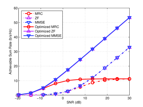
Figure 1: Achievable sum rate of MRC, ZF and MMSE receivers, where $M=20$, $K=4$, $T=196$. Solid lines indicate the sum rate with optimized $\alpha$ and dashed lines illustrate the results with allocating the same power for both training and data phases.

IV-B Degrees of Freedom

We define the DoF of the system as

$$d(M,K,T)\operatorname{:\!=}\sup\lim_{\rho\to\infty}\frac{R^{(\text{total})}(\rho)}{\log_{2}(\rho)}$$ (25)

where the supremum is taken over the totality of all reliable communication schemes for the system, and $R^{(\text{total})}$ denotes the sum rate of the $K$ users under the power constraint $\rho$. We may also speak of the (achieved) degree of freedom of one user for a particular achievability scheme, which is the achieved rate of the user normalized by $\log_{2}(\rho)$ in the limit of $\rho\to\infty$. The DoF measures the multiplexing gain offered by the system when compared to a reference point-to-point single-antenna communication link, in the high SNR regime (see e.g., [12]).

Theorem 2

For an $(M,K,T)$ MIMO uplink system with $M$ receive antennas, $K$ users, and coherence interval $T$, the total DoF of the system is

$$d(M,K,T)=K^{{\dagger}}\left(1-\frac{K^{{\dagger}}}{T}\right).$$ (26)

where $K^{{\dagger}}\operatorname{:\!=}\min(M,K,\lfloor T/2\rfloor)$. $\square$

Proof: To prove the converse, we observe that if we allow the $K$ transmitters to cooperate, then the system is a point-to-point MIMO system with $K$ transmit antennas, $M$ receive antennas, and with no CSI at the receiver. The DoF of this channel has been quantified in [30], in the same form as in the theorem. Without cooperation, the users can at most achieve a rate as high as in the cooperation case.

To prove the achievability, we first look at the case $K^{{\dagger}}<M$. In this case, we note that if we allow only $K^{{\dagger}}$ users to transmit, and let the remaining users be silent, then using the achievability scheme describe in Section III, each of the $K^{{\dagger}}$ users can achieve a rate per user using the zero-forcing receiver given as follows (cf. (20))

$$\left(1-\frac{K^{{\dagger}}}{T}\right)\log_{2}\left(1+\rho_{\text{eff}}(M-K^{{\dagger}})\right).$$ (27)

Note that the condition $K^{{\dagger}}<M$ is needed. If we choose $E=K^{{\dagger}}\rho$ and $\rho_{d}=\rho$, then the effective SNR in (9) becomes

$$\rho_{\text{eff}}=\frac{\rho}{1+\frac{K\rho+1}{K\rho}}.$$ (28)

It can be seen that as $\rho\to\infty$, $\log(\rho_{\text{eff}})/\log(\rho)\to 1$ and a DoF per user of $(1-K^{{\dagger}}/T)$ is achieved. The total achieved DoF is therefore $K^{{\dagger}}(1-K^{{\dagger}}/T)$. Although better energy splitting is possible, as in Section III-C, it will not improve the DoF.

When $K^{{\dagger}}=M$, the case is more subtle. In this case the zero-forcing receive is no longer sufficient. In fact, even the optimal linear processing, which is the MMSE receiver [22, eq. (31)], is not sufficient. The insufficiency can be established by using the results in [7, Sec.IV.C] to show that as $\rho\to\infty$, the effective SNR at the output of MMSE receiver has a limit distribution that is independent of SNR. We skip the details here, since it is not the main concern in this paper.

Instead, we notice that the equivalent channel (7) has SNR given by (28), which for $K\rho>1$ is greater than $\rho/3$. So, the MIMO system can be viewed as a multiple access channel (MAC) with $K^{{\dagger}}$ single-antenna transmitters, and one receiver with $M$ receive antennas. Perfect CSI is known at the receiver, and the SNR between $\rho/3$ and $\rho$. Using the MAC capacity region result [6, Theorem 14.3.1], [26, Sec. 10.2.1], it can be shown that a total DoF of $K^{{\dagger}}$ can be achieved over $T-K^{{\dagger}}$ the time slots.   $\square$

Remark 1. The DoF is the same as that of a point-to-point MIMO channel with $K$ transmit antennas and $M$ receive antennas without transmit- or receive-side CSI [30]. This is a bit surprising because optimal signaling over non-coherent MIMO channel generally requires cooperation among the transmit antennas. It turns out that as far as DoF is concerned, transmit antenna cooperation is not necessary. This is the new twist compared to the point-to-point case.

Remark 2. It can be seen from the achievability proof that for $M>K$, which is generally applicable for massive MIMO systems, ZF at the base station is sufficient for achieving the optimal DoF. However, MRC is not sufficient because $\rho$ shows up both in the numerator and denominator of (19). So as $\rho\to\infty$, the achieved rate is limited. This is due to the interference among the users.

Remark 3. For the case $K^{{\dagger}}=M$, non-linear decoding such as successive interference cancellation is needed.

Remark 4. When $T$ is large, a per-user DoF close to 1 is achievable, as long as $K\leq M$.

Remark 5. When $M$ is larger than $K^{{\dagger}}$, increasing $M$ further has no effect on the DoF. However, it is clear that more receive antennas is useful because more energy is collected by additional antennas. We will discuss the benefit of energy savings in the next section.

IV-C Discussion

IV-C1 Power Savings for Fixed Rate

As more antennas are added to the base station, more energy can be collected. Therefore, it is possible that less energy is needed to be transmitted from the mobile stations. When there is perfect CSI at the base station, it has been shown in [22] that the transmission power can be reduced by a factor $1/M$ to maintain the same rate, compared to a single-user single-antenna system.

When there is no CSI at the receiver, however, it was observed in [22] that the power savings factor is $1/\sqrt{M}$ instead of $1/M$. In the following we do a slightly finer analysis of the effected power savings when $M$ is large, assuming the training phase has been optimized as in Section III.

Consider $M\gg K>1$. Because the received power is linearly proportional to $M$, the transmitted power can be smaller when $M$ is larger. When $M\gg 1$, the system is operating in power-limited regime. It can be seen from (19) and (20) that when $\rho$ is small, MRC performs better than ZF, which has been previously observed, e.g., [22]. On the other hand, in the low-SNR regime the difference between them is a constant factor $(M-1)/(M-K)$ in the SNR term within the logarithmic functions in (19) and (20). The difference becomes negligible when $M$ is large. Using either result, and the effective SNR in (17), we are able to obtain the following.

Corollary 1

If we fix the per-user rate at $R=(1-K/T)\log_{2}(1+\rho_{0})$, then the required power $\rho$ is

$$\rho=\sqrt{\frac{4\rho_{0}(T-K)}{MT^{2}}}+o\left(\frac{1}{\sqrt{M}}\right)$$ (29)

Proof: This can be proved by setting $\rho M=\rho_{0}$ in the rate expression for ZF. Since the achievable rate with ZF processing is worse than MRC and MMSE when SNR is very low, the result is still applied for MRC and MMSE processing.   $\square$

It is interesting to note that increasing $T$ has a similar effect as increasing $M$ on the required transmission power, reducing the power by $1/\sqrt{M}$ or $1/\sqrt{T}$. The reason is the if $T$ is increased, then the energy that can be expended on training is increased, improving the quality of channel estimation. On the other hand, for (29) to be applicable, we need $M\gg K$.

IV-C2 MMSE and Optimal Processing

If MMSE processing is used at the base station, then the performance can be improved compared to MRC and ZF. However, at low SNR, MRC is near optimal and at high SNR, ZF is near optimal. So MMSE processing will not change the nature of the results that we have obtained, although a slightly higher rate is possible. Also, it is observed that the difference between ZF and MMSE is negligible for a wide range of SNR as shown in Figure 1 and the similar results can be found at [22].

IV-C3 Large Scale Fading

When large scale fading is considered, the channel matrix becomes $\mathbf{G}=\mathbf{H}\mathbf{P}$. The matrix $\mathbf{P}=\textrm{diag}\{\sqrt{p_{1}},\ldots,\sqrt{p_{K}}\}\in\mathbb{R}^{K\times K}$ is diagonal where each entry models the path loss and shadow between the base station and the $k$th user. The MMSE estimate of channel is given by $\widehat{\mathbf{G}}=\frac{1}{\sqrt{E}}\mathbf{Y}_{p}(\frac{\mathbf{P}^{-1}}{E}+\mathbf{I})^{-1}$, where the $k$th column of $\widehat{\mathbf{G}}$ is

$$\widehat{\mathbf{G}}_{k}=\frac{p^{\frac{3}{2}}_{k}E}{p_{k}E+1}\mathbf{h}_{k}+\frac{p_{k}\sqrt{E}}{p_{k}E+1}\mathbf{n}_{k}$$ (30)

where $\mathbf{h}_{k}$ and $\mathbf{n}_{k}$ are the $k$th column of $\mathbf{H}$ and $\mathbf{N}$. With the definition of channel estimate error $\widetilde{\mathbf{G}}=\mathbf{G}-\widehat{\mathbf{G}}$, we have the $k$th column of $\widetilde{\mathbf{G}}$, i.e.,

$$\widetilde{\mathbf{G}}_{k}=\mathbf{G}_{k}-\widehat{\mathbf{G}}_{k}=\frac{p_{k}^{\frac{1}{2}}}{p_{k}E+1}\mathbf{h}_{k}-\frac{p_{k}\sqrt{E}}{p_{k}E+1}\mathbf{n}_{k}$$ (31)

where $\mathbf{G}_{k}$ denotes the $k$th column of $\mathbf{G}$. Similar as in Section III-A, we know that the elements of $\widehat{\mathbf{G}}$ and $\widetilde{\mathbf{G}}$ are independent complex Gaussian with zero mean. Also, we can get the variances of each element of $\widehat{\mathbf{G}}_{k}$ and $\widetilde{\mathbf{G}}_{k}$ are

$$\sigma^{2}_{\widehat{\mathbf{G}}_{k}}=\frac{p^{2}_{k}E}{p_{k}E+1}\quad\textrm{and}\quad\sigma^{2}_{\widetilde{\mathbf{G}}_{k}}=\frac{p_{k}}{p_{k}E+1}.$$ (32)

Based on the definition of the equivalent channel in Section III-B, we can obtain the equivalent noise

$$\sigma^{2}_{v}=\sum^{K}_{i=1}\frac{\rho_{d}p_{i}}{p_{i}E+1}+1$$ (33)

and effective SNR of the $k$th user

$$\rho_{\text{eff},k}\operatorname{:\!=} \frac{\rho_{d}\sigma^{2}_{\widehat{\mathbf{G}}_{k}}}{\sigma_{v}^{2}}=\frac{\rho_{d}p^{2}_{k}E}{(p_{k}E+1)(\sum^{K}_{i=1}\frac{\rho_{d}p_{i}}{p_{i}E+1}+1)}$$

$$= \frac{p^{2}_{k}\rho_{d}\rho_{\tau}T_{\tau}}{(p_{k}\rho_{\tau}T_{\tau}+1)(\sum^{K}_{i=1}\frac{\rho_{d}p_{i}}{p_{i}\rho_{\tau}T_{\tau}+1}+1)}.$$ (34)

Then, the corresponding achievable rates can be derived. Specifically, for MRC the following ergodic rate of the $k$th user is achievable:

$$R^{\text{(MRC)}}_{k}\operatorname{:\!=}\left(1-\frac{K}{T}\right)\log_{2}\left(1+\frac{\rho_{\text{eff},k}(M-1)}{\sum^{M}_{i=1,i\neq k}\rho_{\text{eff},i}+1}\right)$$

$$=\left(1-\frac{K}{T}\right)\log_{2}\bigg{(}1+$$

$$\quad\frac{p^{2}_{k}\rho_{d}\rho_{\tau}T_{\tau}(M-1)}{\rho_{d}(p_{k}\rho_{\tau}T_{\tau}+1)\sum^{K}_{i=1,i\neq k}p_{k}+p_{k}(\rho_{d}+\rho_{\tau}T_{\tau})+1}\bigg{)}.$$ (35)

For ZF, assuming $M>K$, the following rate of the $k$th user is achievable:

$$R^{\text{(ZF)}}_{k}\operatorname{:\!=} \left(1-\frac{K}{T}\right)\log_{2}\left(1+\rho_{\text{eff},k}(M-K)\right).$$ (36)

Remark 6. The DoF is not changed when large scale fading is considered. Since we can still choose $E=K^{{\dagger}}\rho$ and $\rho_{d}=\rho$, then the effective SNR in (36) becomes

$$\rho_{\text{eff},k}=\frac{\rho\frac{Kp^{2}_{k}}{Kp_{k}+1/\rho}}{\sum^{K}_{i=1}\frac{p_{i}}{Kp_{i}+1/\rho}+1}.$$ (37)

Similar as in Theorem. 2, when $\rho\to\infty$, $\log(\rho_{\text{eff},k})/\log(\rho)\to 1$ and a DoF per user of $(1-K^{{\dagger}}/T)$ is still achieved.

Remark 7. The convexity of $\rho_{\text{eff},k}$ in terms of $\alpha$ is not easy to prove, but with chosen some special parameters, we can know $\rho_{\text{eff},k}$ is not concave. But it can be proved as quasi-concave. Therefore, the achievable rate can be improved with optimizing $\alpha$ but without global optimal guarantee. However, for the MRC case, the sum achievable rate $\sum^{K}_{k=1}R^{\text{(MRC)}}_{k}$ is concave in terms of $\alpha$ which can be proved easily by Lemma 1 in the Section VI-A. Hence, the optimal $\alpha$ can be also given in both case of average power constraint and peak power constraint.

Remark 8. In a practical system, the channel statistic information is provided from downlink, and adaptive power control mechanism can be adopted for the block fading channel. Since most of the effect of large scale fading can be compensated [9], the power allocation for large scale fading within one coherence interval is not the main issue for the single cell case.

V Joint Optimization of Energy Allocation and Training Duration

If the peak power, rather than the average power, is limited, then our DoF result still holds because the achievability proof actually uses equal power in the training and data transmission phases. The power savings discussion in the previous subsection still applies, because the system is limited by the total amount of energy available, and not how the energy is expended. In the regime where the SNR is neither very high or very low, the peak power constraint will affect the rate. Also, there is a peak power limit for hardware implementation in practical. We provide a detailed analysis in this section.

V-A Energy Allocation

We assume that the transmitters are subject to both peak and average power constraints, where the peak power during the transmission is assumed to be no more than $\rho_{\text{max}}$; i.e.,

$$0\leq\rho_{d},\rho_{\tau}\leq\rho_{\text{max}}.$$ (38)

V-B The Optimization Problem

For an adopted receiver, $\mathcal{A}\in\{\text{MRC},\text{ZF}\}$, our goal is to maximize the uplink achievable rate subject to the peak and average power constraints. Based on the model in (7), we will consider two linear demodulation schemes: MRC and ZF receivers.

For MRC receiver, the received SNR for any of the $K$ users’ symbols can be obtained by substituting $\rho_{\text{eff}}$ into $\rho_{\text{eff}}(M-1)/(\rho_{\text{eff}}(K-1)+1)$ (see [22, eq. (39)]):

$$\textsf{SNR}^{\text{(MRC)}}=\frac{T_{\tau}\rho_{\tau}\rho_{d}(M-1)}{T_{\tau}\rho_{\tau}\rho_{d}(K-1)+K\rho_{d}+T_{\tau}\rho_{\tau}+1}.$$ (39)

For the ZF Receiver, the received SNR for any of the $K$ users’ symbols can be obtained by substituting $\rho_{\text{eff}}$ into $\rho_{\text{eff}}(M-K)$ (see [22, eq. (42)]):

$$\textsf{SNR}^{\text{(ZF)}}=\frac{T_{\tau}\rho_{\tau}\rho_{d}(M-K)}{K\rho_{d}+T_{\tau}\rho_{\tau}+1}.$$ (40)

For either receiver, a lower bound on the sum rate achieved by the $K$ users is given by

$$R^{(\mathcal{A})}(\alpha,T_{d})=\frac{T_{d}}{T}K\log_{2}(1+\textsf{SNR}^{(\mathcal{A})})$$ (41)

where $\mathcal{A}\in\{\text{MRC},\text{ZF}\}$.

Our optimization problem can be formulated as follows:

$$(\textbf{OP})\qquad\mathop{\text{maximize}}_{\alpha,T_{d}}\quad R^{(\mathcal{A})}(\alpha,T_{d})$$ (42)

subject to $$T_{d}+T_{\tau}=T$$ (43)

$$\rho T\alpha+\rho_{\text{max}}T_{d}\leq\rho_{\text{max}}T$$ (44)

$$- \rho T\alpha-\rho_{\text{max}}T_{d}\leq-\rho T$$ (45)

$$0\leq\alpha\leq 1$$ (46)

$$0<T_{d}\leq T-K$$ (47)

where $R^{(\mathcal{A})}(\alpha,T_{d})$ is as given in (41); (44) and (45) are from the peak power constraints in the training and data phases, respectively; and the last constraint is from the requirement that $T_{\tau}\geq K$.

VI SNR Maximization when $T_{d}$ is Fixed

The feasible set of the problem (OP) is convex, but the convexity of the objective function is not obvious. In this section, we consider the optimization problem when $T_{d}$ is fixed. In this case, we will prove that $R^{(\mathcal{A})}(\alpha,T_{d})$ is concave in $\alpha$, and derive the optimized $\alpha$. The result will be useful in the next section where $\alpha$ and $T_{d}$ are jointly optimized.

For a fixed $T_{d}$, from the peak power constraints (44) and (45), we have

$$\frac{\rho_{\text{max}}T_{\tau}}{\rho T}+\left(1-\frac{\rho_{\text{max}}}{\rho}\right)\leq\alpha\leq\frac{\rho_{\text{max}}T_{\tau}}{\rho T}.$$ (48)

Combined with (46), the overall constraints on $\alpha$ are

$$\min\{0,\frac{\rho_{\text{max}}T_{\tau}}{\rho T}+\left(1-\frac{\rho_{\text{max}}}{\rho}\right)\}\leq\alpha\leq\max\{\frac{\rho_{\text{max}}T_{\tau}}{\rho T},1\}.$$ (49)

In the remaining part of this section, we will first ignore the peak power constraint, and derive the optimal $\alpha\in(0,1)$ for a given $T_{d}$. At the end of this section, we will reconsider the effect of the peak power constraint on the optimal $\alpha$.

VI-A MRC Case without Peak Power Constraint

Using (10) we can rewrite (39) as

$$\textsf{SNR}^{\text{(MRC)}}(\alpha)=\frac{M-1}{K-1}\frac{\alpha(\alpha-1)}{\alpha^{2}-a_{1}\alpha-b_{1}}$$ (50)

where

$$a_{1}=1+\frac{T_{d}-K}{\rho T(K-1)},\quad b_{1}=\frac{\rho TK+T_{d}}{\rho^{2}T^{2}(K-1)}>0.$$ (51)

It can be verified that $1-a_{1}-b_{1}\leq 0$.

VI-A1 Behavior of the $\textsf{SNR}^{\text{(MRC)}}(\alpha)$ Function

Define

$$g(\alpha):=\textsf{SNR}^{\text{(MRC)}}\cdot(K-1)/(M-1).$$ (52)

And let $g_{d}(\alpha)=\alpha^{2}-a_{1}\alpha-b_{1}$, which is the denominator of $g(\alpha)$.

Lemma 1

The function $g(\alpha)$ is concave in $\alpha$ over $(0,1)$ when $1-a_{1}-b_{1}\leq 0$ and $b_{1}>0$.

Proof: See Appendix A.   $\square$

Lemma 1 gives the convex conditions of the objective function. According to Lemma 1, we know that there is a global maximal point for (50). Taking the derivative of (50) and setting it as 0, we have

$$(1-a_{1})\alpha^{2}-2b_{1}\alpha+b_{1}=0.$$ (53)

Remark 9. It can be observed that when $1-a_{1}-b_{1}\leq 0$ and $b_{1}>0$, $g_{d}(\alpha)$ is non-positive at both $\alpha=0$ and $\alpha=1$. Since the leading coefficient of $g_{d}(\alpha)$ is positive, $g_{d}(\alpha)<0$ for $\alpha\in(0,1)$, and it has no root in $(0,1)$.

Based on Remark 1, we deduce that $g(\alpha)>0$ for $\alpha\in(0,1)$. In addition, we have $g(0)=0$ and $g(1)=0$. Therefore, there is an optimal $\alpha$ within $(0,1)$ rather than at boundaries.

VI-A2 The Optimizing $\alpha$

We discuss the optimal $\alpha$ in three cases, depending on $T_{d}$, as compared to $K$.

• If $T_{d}=K$, then $1-a_{1}=0$. Hence, we have $\alpha^{*}=1/2$, and

  $$\textsf{SNR}^{\text{(MRC)}}(\frac{1}{2})=\frac{M-1}{K-1}\frac{1/4}{1/4+\frac{K(\rho T+1)}{\rho^{2}T^{2}(K-1)}}$$ (54)

• If $T_{d}<K$, then $1-a_{1}>0$. Since $b_{1}>1-a_{1}$, $b_{1}/(1-a_{1})>1$. Between the two roots of (53), the one in between 0 and 1 is

  $$\alpha^{*}=\frac{b_{1}-\sqrt{b_{1}(a_{1}+b_{1}-1)}}{1-a_{1}}.$$ (55)

• If $T_{d}>K$, then $1-a_{1}<0$. It can be deduced that in this case $\alpha^{*}$ in (55) is still between 0 and 1 and therefore is the optimal $\alpha$.

Substituting (51) into (55), we have

$$\alpha^{*}=\frac{\sqrt{(\rho TK+T_{d})(\rho TT_{d}+T_{d})}-(\rho TK+T_{d})}{\rho T(T_{d}-K)}.$$ (56)

We can simplify the expression for the optimal $\alpha$ at high and low SNR:

• At high SNR, the optimal $\alpha^{*}$ is

  $$\alpha^{*}_{\rm H}\approx\frac{\sqrt{KT_{d}}-K}{T_{d}-K}=\frac{\sqrt{K}}{\sqrt{T_{d}}+\sqrt{K}}.$$ (57)

• Similarly, at low SNR, the optimal $\alpha^{*}$ is

  $$\alpha^{*}_{\rm L}\approx\frac{1}{2}.$$ (58)

  As a result, $\textsf{SNR}^{\text{(MRC)}}(\alpha^{*}_{\rm L})=(M-1)/(4T_{d}(K-1))$. If the SNR is low, the fraction between the training and data is independent on the system parameters $M$, $K$, $\rho_{d}$, $\rho_{\tau}$, $T_{\tau}$, and $T$.

VI-B ZF Case without Peak Power Constraint

This optimization problem in the ZF case is similar to that in Section. III-C. Here, we only give the final optimization results.

Using (10) we can rewrite (40) as

$$\textsf{SNR}^{\text{(ZF)}}(\alpha)=\frac{\rho T(M-K)\alpha(1-\alpha)}{(T_{d}-K)(\gamma+\alpha)}$$ (59)

The optimized results of $\alpha^{*}$ are the same as in (12). The optimized $\textsf{SNR}^{\text{(ZF)}}$ is just given by $(M-K)\rho_{\text{eff}}^{*}$. At both high SNR and low SNR, the results are the same as in the MRC case.

VI-C MRC and ZF with Peak Power Constraint

So far we have ignored the peak power constraint. When the peak power is considered, and $\alpha^{*}$ is not within the feasible set (49), the optimal $\widetilde{\alpha}^{*}$ with the peak power constraint is the $\alpha$ within the feasible set that is closest to the $\alpha^{*}$ we derived, which is at one of the two boundaries of the feasible set, due to the concavity of the objective function.

VII Achievable Rate Maximization in General

In this section, $\alpha$ and $T_{d}$ are jointly optimized for maximizing the achievable rate of uplink MU-MIMO system as illustrated in (42)–(47) when both average and peak power constraints are considered.

The feasible set with respective to $\alpha$ and $T_{d}$ is illustrated in Fig. 2. It can be observed that the feasible region is in between the following two lines

$$T_{d} = -\rho T\alpha/\rho_{\text{max}}+T,$$ (60)

$$T_{d} = -\rho T\alpha/\rho_{\text{max}}+\rho T/\rho_{\text{max}}$$ (61)

where $\alpha$ and $T_{d}$ satisfy (46) and (47).

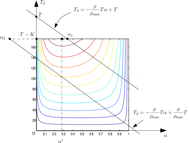
Figure 2: Feasible region and the contour of the objective function in the MRC case; $T=196$, $K=20$ and $M=50$.

We have the following lemma that is useful for describing the behavior of our objective function $R^{(\mathcal{A})}(\alpha,T_{d})$ when $\alpha$ is fixed.

Lemma 2

The function $f(x)=x\ln(1+a/(b+cx))$, when $a,b,c,x>0$, is concave and monotonically increasing.

Proof: See Appendix B.   $\square$

In summary, the convexity of the objective function is known to have the following two properties:

1. From Lemma 1, for fixed $T_{d}$, $R^{(\mathcal{A})}$ is a concave function with respect to $\alpha$.

2. From Lemma 2, for fixed $\alpha$, $R^{(\mathcal{A})}$ is a concave function and monotonically increasing with respect to $T_{d}$.

Since the feasible set is convex, our optimization problem (OP) is a biconvex problem that may include multiple local optimal solutions. However, after studying the convexity of the objective function, there are only three possible cases for the optimal solutions, as we discuss below.

In the remainder of this section, let $\alpha^{\dagger}$ denote the optimal $\alpha$ when $T_{d}=T-K$, which is given by Section VI-A and Section VI-B for MRC and ZF processing.

VII-A Case 1: $\rho_{\tau}$ is limited by $\rho_{\text{max}}$

Define $\alpha_{1}:=\rho_{\text{max}}K/\rho T$, which is the root of $T-K=-\rho T\alpha/\rho_{\text{max}}+T$ in $\alpha$ (see Fig. 2). In the case where $\alpha_{1}<\alpha^{\dagger}$, because of the property P2 the optimal $(\alpha^{*},T_{d}^{*})$ must be on one of the two lines given by i) $T_{d}=-\rho T\alpha/\rho_{\text{max}}+T$, $\alpha\in[\alpha_{1},1]$, and ii) $T_{d}=T-K$, $\alpha\in[0,\alpha_{1}]$.

On the line $T_{d}=T-K,\alpha\in[0,\alpha_{1}]$ the objective function is concave and increasing with $\alpha$, thanks to property P1. Hence, we only need to consider the line $T_{d}=-\rho T\alpha/\rho_{\text{max}}+T,\alpha\in[\alpha_{1},1]$.

Lemma 3

The objective function $R^{(\text{MRC})}(\alpha,T_{d})$ along the line $T_{d}=-\rho T\alpha/\rho_{\text{max}}+T,\alpha\in[\alpha_{1},1]$ is quasiconcave in $\alpha$.

Proof: Consider MRC processing. Substituting (60) into $R^{(\text{MRC})}(\alpha,T_{d})$, we have

$$R^{\text{(MRC)}}(\alpha)=\frac{K}{T}\left(-\frac{\rho T}{\rho_{\text{max}}}\alpha+T\right)\log_{2}(1+\textsf{SNR}^{\text{(MRC)}}(\alpha))$$ (62)

where

$$\textsf{SNR}^{\text{(MRC)}}(\alpha)=\frac{\alpha(\alpha-1)\rho^{2}T^{2}(M-1)}{a_{2}\alpha^{2}-b_{2}\alpha-c_{2}},$$ (63)

and $a_{2}=\rho^{2}T^{2}(K-1)+\rho^{2}T^{2}/\rho_{\text{max}}$, $b_{2}=\rho^{2}T^{2}(K-1)+\rho T^{2}-\rho TK-\rho T/\rho_{\text{max}}$ and $c_{2}=K\rho T+T$. Since $R^{\text{(MRC)}}(\alpha)>0$, in order to prove the quasi-concavity of $R^{\text{(MRC)}}(\alpha)$, we need to prove that the super-level set $\mathcal{S}_{\beta}=\{\alpha|0<\alpha<1,R^{\text{(MRC)}}(\alpha)\geq\beta\}$ for each $\beta\in\mathbb{R}^{+}$ is convex. Equivalently, if we define

$$\phi_{\beta}(\alpha)=\frac{\beta}{\frac{K}{T}(\frac{\rho T\alpha}{\rho_{\text{max}}}-T)}+\log_{2}(1+\textsf{SNR}^{\text{(MRC)}}(\alpha)).$$ (64)

we only need to prove that $\mathcal{S}_{\phi}=\{\alpha|0<\alpha<1,\phi_{\beta}(\alpha)\geq 0\}$ is a convex set.

It can be checked that the first part of $\phi_{\beta}(\alpha)$, namely $\beta/[{\frac{K}{T}(\frac{\rho T\alpha}{\rho_{\text{max}}}-T)}]$, is concave for $\alpha\in[0,1]$. For the other part of $\phi_{\beta}(\alpha)$, from (63) we know that

$$a_{2}-b_{2}-c_{2}=\rho T(\frac{\rho}{\rho_{\text{max}}}-1)-T(1-\alpha\frac{\rho}{\rho_{\text{max}}})<0$$ (65)

where $a_{2},c_{2}>0$. Applying Lemma 1, we know $\textsf{SNR}^{\text{(MRC)}}(\alpha)$ is concave. Hence, $\log_{2}(1+\textsf{SNR}^{\text{(MRC)}}(\alpha))$ is also concave since function $\log(1+x)$ is concave and non-decreasing [5]. Therefore, its super-level set $\mathcal{S}_{\phi}$ is convex. It follows that the super-level set $\mathcal{S}_{\beta}$ of $R^{\text{(MRC)}}(\alpha)$ is convex for each $\beta\geq 0$. The objective function is thus quasiconcave.   $\square$

Thanks to Lemma 3, we can find the optimal $\alpha$ by setting the derivative of (62) with respect to $\alpha$ to 0. Efficient one-dimensional searching algorithm such as Newton method or bisection algorithm [5], can be adopted to find out the optimal $\alpha$.

VII-B Case 2: $\rho_{d}$ is limited by $\rho_{\text{max}}$

Define $\alpha_{2}:=1-\rho_{\text{max}}(T-K)/\rho T$, which is the root of $T-K=\rho T\alpha/\rho_{\text{max}}+\rho T/\rho_{\text{max}}$ in $\alpha$. If $\alpha_{2}>\alpha^{\dagger}$, because of the property P2 the optimal $(\alpha^{*},T_{d}^{*})$ must be on one of the two lines given by i) $T_{d}=-\rho T\alpha/\rho_{\text{max}}+T,\alpha\in(\alpha_{1},1)$, $\alpha\in[\alpha_{1},1]$, and ii) $T_{d}=T-K$, $\alpha\in[\alpha_{2},\alpha_{1}]$. Along the line $T_{d}=T-K,\alpha\in(\alpha_{1},1)$, the corresponding function is decreasing in $\alpha$ because of the property P1. Also considering P2, which implies that the optimal point in this case cannot include $T_{d}<T-K$, we conclude that the point $(\alpha^{*},T_{d}^{*})=(\alpha_{2},T-K)$ is the global optimal solution of the problem.

VII-C Case 3: Both $\rho_{d}$ and $\rho_{\tau}$ are not limited by $\rho_{\text{max}}$

If $\alpha_{2}<\alpha^{\dagger}<\alpha_{1}$, the optimal point is achieved at $(\alpha^{*},T_{d}^{*})=(\alpha^{\dagger},T-K)$, according to properties P1 and P2.

Summarizing what we have discussed so far, we have the following theorem.

Theorem 3

For the MRC receiver, set $\alpha^{\dagger}=1/2$ if $T_{d}=K$ and otherwise set $\alpha^{\dagger}$ according to (56) when $T_{d}=T-K$. Set $\alpha_{1}=\rho_{\text{max}}K/\rho T$ and set $\alpha_{2}=1-\rho_{\text{max}}(T-K)/\rho T$. The solution for the joint optimization of training energy allocation $\alpha$ and the training duration $T_{\tau}=T-T_{d}$ is given in three cases. Case 1) If $\alpha_{1}<\alpha^{\dagger}$, then $\alpha^{*}$ is given by the maximizer of $R^{(\text{MRC})}(\alpha)$ in (62), and $T_{d}^{*}=-\rho T\alpha^{*}/\rho_{\text{max}}+T$; Case 2) If $\alpha_{2}>\alpha^{\dagger}$ then $(\alpha^{*},T_{d}^{*})=(\alpha_{2},T-K)$; Case 3) If $\alpha_{2}<\alpha^{\dagger}<\alpha_{1}$, then $(\alpha^{*},T_{d}^{*})=(\alpha^{\dagger},T-K)$.

We also have similar results regarding the optimal energy allocation factor $\alpha$ and training period $T_{\tau}$ for the ZF case. The only difference is that the achievable rate $R^{\text{(ZF)}}(\alpha)$ should be given by substituting (60) into $R^{(\text{ZF})}(\alpha,T_{d})$, which is

$$R^{\text{(ZF)}}(\alpha)=\frac{K}{T}\left(-\frac{\rho T}{\rho_{\text{max}}}\alpha+T\right)\log_{2}(1+\textsf{SNR}^{\text{(ZF)}}(\alpha))$$ (66)

where

$$\textsf{SNR}^{\text{(MRC)}}(\alpha)=\frac{\alpha(\alpha-1)\rho^{2}T^{2}(M-K)}{a_{3}\alpha^{2}-b_{3}\alpha-c_{3}},$$ (67)

and $a_{3}=\rho^{2}T^{2}/\rho_{\text{max}}$, $b_{3}=\rho T^{2}-\rho TK-\rho T/\rho_{\text{max}}$ and $c_{3}=K\rho T+T$. Comparing (62), (63) and (66), (67), we can obtain the results for ZF receiver as follows.

Theorem 4

For the ZF receiver, set $\alpha^{\dagger}=1/2$ if $T_{d}=K$ and otherwise set $\alpha^{\dagger}$ according to (12) when $T_{d}=T-K$. Set $\alpha_{1}=\rho_{\text{max}}K/\rho T$ and set $\alpha_{2}=1-\rho_{\text{max}}(T-K)/\rho T$. The solution for the joint optimization of training energy allocation $\alpha$ and the training duration $T_{\tau}=T-T_{d}$ is given in three cases. Case 1) If $\alpha_{1}<\alpha^{\dagger}$, then $\alpha^{*}$ is given by the maximizer of $R^{(\text{ZF})}(\alpha)$ in (66), and $T_{d}^{*}=-\rho T\alpha^{*}/\rho_{\text{max}}+T$; Case 2) If $\alpha_{2}>\alpha^{\dagger}$ then $(\alpha^{*},T_{d}^{*})=(\alpha_{2},T-K)$; Case 3) If $\alpha_{2}<\alpha^{\dagger}<\alpha_{1}$, then $(\alpha^{*},T_{d}^{*})=(\alpha^{\dagger},T-K)$.

We also remark that our results are applicable for any $M>K$, including when $M\gg K$, i.e., the massive MIMO system case.

VIII Discussion

When $M$ increases, the transmit power of each user can be reduced proportionally to $1/\sqrt{M}$ for large $M$ while maintaining a fixed rate as discussed in Section IV-C1 and [22]. Here we discuss the asymptotic achievable rates when $M\to\infty$.

VIII-A Optimized $\alpha$ if $T_{d}$ is fixed when $M\to\infty$

If the energy over the training and data phases is allocated differently, we have the following results after optimizing the $\alpha$ for large $M$.

Theorem 5

For both ZF and MRC, let $\rho_{u}:=\sqrt{M}\rho$ be fixed. Then, the maximum achievable rate can be

$$R^{(\mathcal{A})}\rightarrow\frac{T_{d}}{T}K\log_{2}(1+\frac{\rho_{u}^{2}T^{2}}{4T_{d}}),\quad M\to\infty$$ (68)

Proof: According to (50) and (59), when $M\to\infty$, we have

$$\textsf{SNR}^{(\mathcal{A})}(\alpha)=\frac{\alpha(1-\alpha)\rho_{u}^{2}T^{2}}{T_{d}},$$ (69)

where the maximum received SNR can be obviously obtained when $\alpha=1/2$.   $\square$

Note, if the peak power constraints are considered, $\alpha$ needs to be within the interval as shown in (49). Otherwise, the optimal solution is located at the boundary of (49).

Remark 10. If the power is allocated equally between the two phases, we have $\alpha=T_{\tau}/T$ [22], then the difference of achievable rate between the optimized and the equally allocated power scheme is

$$\Delta R^{(\mathcal{A})}(\alpha) =\frac{T_{d}}{T}K(\log_{2}(1+\frac{\rho^{2}_{u}T^{2}}{4T_{d}})-\log_{2}(1+T_{\tau}\rho^{2}_{u})),$$

$$=\frac{T_{d}}{T}K\log_{2}(\frac{4T_{d}+\rho^{2}_{u}T^{2}}{4T_{d}+4T_{d}(T-T_{d})\rho^{2}_{u}}),$$ (70)

where the numerator minus the denominator within the $\log_{2}(\cdot)$ is equal to $\rho^{2}_{u}(T^{2}-4TT_{d}+T_{d}^{2})=\rho^{2}_{u}(T-T_{d})^{2}\geq 0$. Therefore, it is clear that the optimized achievable rate is always larger than the unoptimized one. The gain in rate offered by optimizing the energy allocated for training is given by (70).

VIII-B Optimized $\alpha$ and $T_{d}$ when $M\to\infty$

For both MRC and ZF, under the peak power constraints, the average transmit power of each user is $\rho=\rho_{u}/\sqrt{M}$, where $\rho_{u}$ is fixed. Define $\rho/\rho_{\max}=\xi$. Consequently, the corresponding $\rho_{\max}=\rho_{u}/(\xi\sqrt{M})$. When $M\to\infty$, applying Theorems 3 and 4, we have the following cases:

• Case 1: $\rho_{\tau}$ is limited by $\rho_{\text{max}}$

  $$R^{(\mathcal{A})}(\alpha)=K(-\xi\alpha+1)\log_{2}\left(1+\frac{\alpha(\alpha-1)\rho_{u}^{2}T}{\xi\alpha-1}\right)$$ (71)

  Taking the derivative of (71) and setting it to zero, we can obtain the optimal $\alpha$ with one dimension search algorithm [5]. Then, the duration $T^{*}_{d}$ can be obtained by (60) directly with substituting $\alpha^{*}$.

• Case 2: $\rho_{d}$ is limited by $\rho_{\text{max}}$

  $$R^{(\mathcal{A})}(\alpha^{*})=K\xi(-\alpha^{*}+1)\log_{2}\left(1+\frac{\alpha^{*}(\alpha^{*}-1)\rho^{2}_{u}T}{T-K}\right)$$ (72)

  where $\alpha^{*}=1-(T-K)/(\xi T)$ and $T^{*}_{d}=T-K$.

• Case 3: Neither $\rho_{d}$ nor $\rho_{\tau}$ is not limited by $\rho_{\text{max}}$

  $$R^{(\mathcal{A})}(\alpha^{*})=\frac{T-K}{T}K\log_{2}\left(1+\frac{\rho_{u}^{2}T^{2}}{4(T-K)}\right)$$ (73)

  where $\alpha^{*}=1/2$ and $T_{d}^{*}=T-K$.

IX Numerical Results

In this section, we compare the achievable rates between equal power allocation scheme and our optimized one under average and peak power constraints. In our simulations, we set $\rho_{\max}=1.2\rho$, $K=10$, and $T=196$. We consider the following schemes: 1) MRC, which refers to the case where MRC receiver is used and the same average power is used in both training and data transmission phases [22]. 2) A-MRC, which refers to the case where MRC receiver is used, the training duration is $K$, and there is only average power constraint. 3) AP-MRC, where MRC receiver is used, and both the training duration and training energy are optimized under both the average and peak power constraints. We will also consider the ZF variants of the above three cases, namely ZF, A-ZF, and AP-ZF. The energy efficiency is defined as $\eta^{\mathcal{A}}:=R^{\mathcal{A}}(\alpha,T_{d})/\rho$.

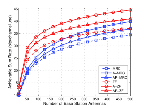
Figure 3: Comparison between equal and optimized power allocations when the number of base station antennas increases; $\rho_{u}=3$dB.

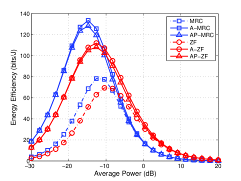
Figure 4: Comparison of energy efficiency for different SNR $\rho$; where $M=30$.

In Fig. 3, we show the achieved rates of various schemes as the number of antennas increases. It can be seen that the A-MRC (ZF) performs better than the MRC (ZF) as well as the AP-MRC (ZF). In Fig. 4, the energy efficiency is shown as a function of $\rho$. It can be seen that there is an optimal average transmitted power for maximum energy efficiency as has been also observed before in [22]. It can also be seen that optimized schemes, e.g., A-MRC (A-ZF) and AP-MRC (AP-ZF), show a significant gain when SNR is low, since the power resource is scarce. Thus, the optimization of power allocation and training duration plays much more important role when $\rho$ is small than the case when $\rho$ is large. In Fig. 5, we show the energy efficiency versus sum rate. In particular, the optimized schemes achieve higher energy efficiencies. Also from the simulations, we can see that ZF performs better than MRC at high SNR, but worse when SNR is low.

Moreover, the impact of peak power constraint on achievable rates and energy efficiencies for both MRC and ZF receivers can be observed through from Fig. 3 to Fig. 5 clearly. They illustrate that when peak power is limited at the training phase, the achievable rate with AP-MRC and AP-ZF cannot be as high as the case with A-MRC and ZF. Although the training period is increased, the time slot is still very precious when the achievable rate needs to be maximized. In addition, we give an example about energy efficiency versus the peak power limit in Fig. 6. It can be observed that as the power limit increases, the energy efficiency with AP-MRC and AP-ZF approaches the one with A-MRC and A-ZF, meaning that the channel can be estimated accurately and more time slots are allocated to the data phase.

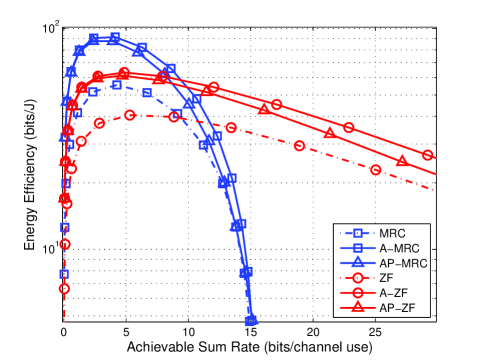
Figure 5: Comparison of energy efficiency versus the achievable sum rate, where $M=20$.

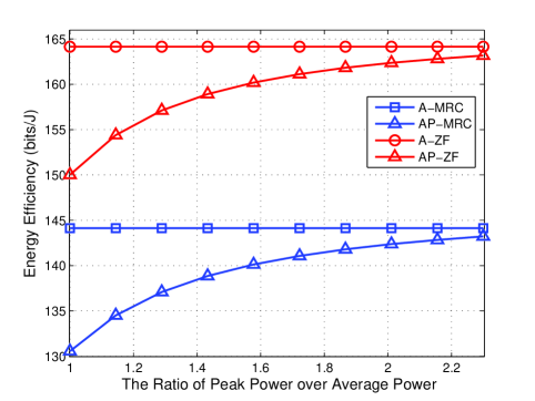
Figure 6: Comparison of energy efficiency versus the ratio of peak power over average power, where $M=50$ and $\rho=-10$dB.

X Conclusions

In this paper, we considered an uplink multiuser cellular system where the base station is equipped with multiple antennas. The channels were assumed to be acquired by the base station through training symbols transmitted by the mobile users. With estimated channels at the base station, we derived sum rates that is achievable with MMSE channel estimation and MRC, ZF, and MMSE detectors. Based on the derived rates, we were able to quantify the amount of energy savings that are possible through the increase of either the number of base station antennas, or the coherence interval length. We also quantified the degrees of freedom that is possible in this scenarios, which is the same as that of a point-to-point MIMO system. The achievability scheme when the number of users is less than the number of base station antennas is linear: zero-forcing is sufficient. Otherwise, nonlinear processing at the base station is necessary to achieve the optimal total degrees of freedom.

For the case that both average and peak power constraints were considered, we considered the problem of joint training energy and training duration optimization for the MRC and ZF receivers so that the sum achievable rate is maximized. We also performed a careful analysis of the convexity of the problem and derived optimal solutions either in closed forms or in one case through a one-dimensional search of a quasi-concave function. Our results were illustrated and verified through numerical examples.

The effect of pilot contamination for multi-cell setup should also be the importance influence on the achievable sum rate where the large scale fading would be one of the main concerns, which will be considered as the future work.

XI Appendix

XI-A Proof of Lemma 1

Replacing $\alpha$ as $x$ in (50), we need to verify that the second derivative of (50) with respective to $x$ is negative [5]. The first derivative of $g(x)$ is

$$g^{\prime}(x)=\frac{(1-a)x^{2}-2bx+b}{(x^{2}-ax-b)^{2}}$$ (74)

where $1-a-b<0$, $b>0$ and $x\in(0,1)$. Then, taking the second derivative of $g(x)$, we have

$$g^{\prime\prime}(x)=\frac{2}{(x^{2}-ax-b)^{3}}\underbrace{\big{(}(a-1)x^{3}+3bx^{2}-3bx+ab+b^{2}\big{)}}_{f(x)}$$ (75)

From Remark 1 and $b>0$, we know that $(x^{2}-ax-b)^{3}<0$. We need to show $f(x)>0$.

Checking the boundary of $f(x)$, we know that

$$f(0)=ab+b^{2}=b(b+a)>b>0,$$ (76)

$$f(1)=ab+b^{2}=a-1+ab+b^{2}=(a+b-1)(b+1)>0.$$ (77)

Next, we need to consider the monotonicity of the function during the interval $x\in(0,1)$. Taking the derivative of $f(x)$, we get

$$f^{\prime}(x)= 3(a-1)x^{2}+6bx-3b$$

$$=3(a-1)(x^{2}+\frac{2b}{a-1}x-\frac{b}{a-1}),$$ (78)

which is a quadratic function.

When $a=1$, $f^{\prime}(x)=6bx-3b=3b(2x-1)$. The function is decreasing until $x=1/2$ and increasing afterwards. Since

$$f(\frac{1}{2})=\frac{1}{4}b+b^{2}>0,$$ (79)

it can be deduced that $f(x)>0$.

When $a\neq 1$, we know that $f^{\prime}(1)=3(a+b-1)>0$, $f^{\prime}(0)=-3b$, meaning that the function $f(x)$ is decreasing first and increasing after the minimum point.

Here, we need to verify the minimum value of $f(x^{*})$ is always greater than 0. According to (XI-A), the minimum point given by the root of $f^{\prime}(x^{*})=0$ is

$$x^{*}=-\frac{b}{a-1}+\sqrt{\frac{b(a+b-1)}{(a-1)^{2}}},$$ (80)

since $a+b>1$ and $b>0$. Substituting (80) into $f(x)$, we have

$$f(x^{*})= [x((a-1)x^{2}+2bx-b)+bx^{2}-2bx+ab+b^{2}]\bigr{|}_{x=x^{*}}$$

$$= \frac{b(a+b-1)}{a-1}\underbrace{(\frac{2b}{a-1}-2\sqrt{\frac{b(a+b-1)}{(a-1)^{2}}}+a)}_{h}.$$ (81)

For $a-1>0$,

$$h= \frac{2b}{a-1}-\frac{\sqrt{b(a+b-1)}}{a-1}+a$$

$$= \frac{2}{a-1}\frac{b^{2}-b(a+b-1)}{b+\sqrt{b(a+b-1)}}+a$$ (82)

$$\mathop{>}\limits^{(a)} a-\frac{2b}{b+\sqrt{b^{2}}}>0$$ (83)

where (a) is based on $a-1>0$. Therefore, $f(x)>0$.

For $a-1<0$,

$$h =\frac{2b}{a-1}+\frac{2\sqrt{b(a+b-1)}}{a-1}+a$$ (84)

$$\mathop{<}^{(b)}\frac{2(1-a)}{a-1}+a<0,$$ (85)

where (b) is due to $b>1-a$. Hence, $f(x)>0$.

XI-B Proof of Lemma 2

The derivative of $f(x)=x\ln(1+a/(b+cx))$, where $a,b,c,x>0$, is

$$f^{\prime}(x)=\ln(1+\frac{a}{cx+b})-\frac{acx}{(cx+a+b)(cx+b)}$$ (86)

It is clear that $\lim_{x\to\infty}f^{\prime}(x)=0$. If we can verify that the function $f^{\prime}(x)$ is monotonically decreasing, then $f^{\prime}(x)$ is always positive. Hence, we take the derivative of $f^{\prime}(x)$, and obtain

$$f^{\prime\prime}(x)=-\frac{abc^{2}x+ac^{2}(a+b)x+2ac(a+b)b}{[(cx+b)(cx+a+b)]^{2}}<0,$$ (87)

since $a,b,c,x>0$. This means that $f^{\prime}(x)$ is decreasing. Therefore, $f^{\prime}(x)$ is always positive, i.e., $f(x)$ is an increasing and concave function.

References

- [1] T. Bai and R. W. H. Jr., “Analyzing uplink SIR and rate in massive MIMO systems using stochastic geometry,” CoRR, vol. abs/1510.02538, 2015.
- [2] I. Bergel, Y. Perets, and S. Shamai, “Uplink downlink rate balancing and throughput scaling in FDD massive MIMO systems,” CoRR, vol. abs/1507.03762, 2015.
- [3] E. Bjornson, J. Hoydis, M. Kountouris, and M. Debbah, “Massive MIMO systems with non-ideal hardware: Energy efficiency, estimation, and capacity limits,” IEEE Trans. Info. Theory, vol. 60, no. 11, pp. 7112–7139, Nov 2014.
- [4] E. Bjornson, M. Matthaiou, and M. Debbah, “Massive MIMO with non-ideal arbitrary arrays: Hardware scaling laws and circuit-aware design,” arXiv:1409.0875 [cs.IT], 2014.
- [5] S. Boyd and L. Vandenberghe, Convex Optimization, Cambridge University Press, 2004.
- [6] T. M. Cover and J. A. Thomas, Elements of Information Theory, John Wiley & Sons, Inc., 1991.
- [7] H. Gao, P. J. Smith, and M. V. Clark, “Theoretical reliability of MMSE linear diversity combining in Rayleigh-fading additive interference channels,” IEEE Trans. Commun., vol. 46, no. 5, pp. 666–672, May 1998.
- [8] M. Gkizeli and G. Karystinos, “Maximum-SNR antenna selection among a large number of transmit antennas,” IEEE J. Sel. Topics Signal Process., vol. 8, no. 5, pp. 891–901, Oct. 2014.
- [9] A. Goldsmith, Wireless Communications, Cambridge University Press, 2005.
- [10] B. Hassibi, M. Hansen, A. Dimakis, H. Alshamary, and W. Xu, “Optimized Markov chain Monte Carlo for signal detection in MIMO systems: An analysis of the stationary distribution and mixing time,” IEEE Trans. Signal Process., vol. 62, no. 17, pp. 4436–4450, Sept. 2014.
- [11] B. Hassibi and B. M. Hochwald, “How much training is needed in multiple-antenna wireless links?” IEEE Trans. Info. Theory, vol. 49, no. 4, pp. 951–963, Apr. 2003.
- [12] S. A. Jafar, “Interference alignment: A new look at signal dimensions in a communication network,” Foundations and Trends in Communications and Information Theory, vol. 7, no. 1, pp. 1–134, 2010.
- [13] J. Jose, A. Ashikhmin, T. Marzetta, and S. Vishwanath, “Pilot contamination and precoding in multi-cell TDD systems,” IEEE Trans. Wireless Commun., vol. 10, no. 8, pp. 2640–2651, Aug. 2011.
- [14] M. Kobayashi, N. Jindal, and G. Caire, “Training and feedback optimization for multiuser MIMO downlink,” IEEE Trans. Commun., vol. 59, no. 8, pp. 2228–2240, Aug. 2011.
- [15] E. Larsson, O. Edfors, F. Tufvesson, and T. Marzetta, “Massive MIMO for next generation wireless systems,” IEEE Commun. Mag., vol. 52, no. 2, pp. 186–195, Feb. 2014.
- [16] S. Lu and Z. Wang, “Achievable rates of uplink multiuser massive MIMO systems with estimated channels,” in Proc. of IEEE Global Communications Conference (GLOBECOM), Austin, USA, pp. 3772–3777, Dec. 2014.
- [17] S. Lu and Z. Wang, “Joint optimization of power allocation and training duration for uplink multiuser MIMO communications,” in Proc. of IEEE Wireless Communications and Networking Conference (WCNC), New Orleans, USA, pp. 322–327, Mar. 2015.
- [18] M. R. McKay, I. B. Collings, and A. M. Tulino, “Achievable sum rate of MIMO MMSE receivers: A general analytic framework,” IEEE Trans. Info. Theory, vol. 56, no. 1, pp. 396–410, Jan. 2010.
- [19] G. Miao, “Energy-efficient uplink multi-user MIMO,” IEEE Trans. Wireless Commun., vol. 12, no. 5, pp. 2302–2313, May 2013.
- [20] S. Mohammed and E. Larsson, “Per-antenna constant envelope precoding for large multi-user MIMO systems,” IEEE Trans. Commun., vol. 61, no. 3, pp. 1059–1071, Mar. 2013.
- [21] H. Q. Ngo, E. G. Larsson, and T. L. Marzetta, “The multicell multiuser MIMO uplink with very large antenna arrays and a finite-dimensional channel,” IEEE Trans. Commun., vol. 61, no. 6, pp. 2350–2361, June 2013.
- [22] H. Q. Ngo, E. G. Larsson, and T. L. Marzetta, “Energy and spectral efficiency of very large multiuser MIMO systems,” IEEE Trans. Commun., vol. 61, no. 4, pp. 1436–1449, Apr. 2013.
- [23] H. Ngo, M. Matthaiou, and E. Larsson, “Massive MIMO with optimal power and training duration allocation,” IEEE Wireless Commun. Lett., vol. 3, no. 6, pp. 605–608, Dec 2014.
- [24] S. Noh, M. Zoltowski, Y. Sung, and D. Love, “Pilot beam pattern design for channel estimation in massive MIMO systems,” IEEE J. Sel. Topics Signal Process., vol. 8, no. 5, pp. 787–801, Oct. 2014.
- [25] F. Rusek, D. Persson, B. K. Lau, E. G. Larsson, T. L. Marzetta, O. Edfors, and F. Tufvesson, “Scaling up MIMO: opportunities and challenges with very large arrays,” IEEE Signal Process. Mag., vol. 30, no. 1, pp. 40–60, Jan. 2013.
- [26] D. Tse and P. Viswanath, Fundamentals of Wireless Communication, Cambridge University Press, 2005.
- [27] G. Yang, C. K. Ho, R. Zhang, and Y. L. Guan, “Throughput optimization for massive MIMO systems powered by wireless energy transfer,” IEEE J. Select. Areas Commun., vol. 33, no. 8, pp. 1640–1650, 2015.
- [28] H. Yang and T. Marzetta, “Performance of conjugate and zero-forcing beamforming in large-scale antenna systems,” IEEE J. Select. Areas Commun., vol. 31, no. 2, pp. 172–179, Feb. 2013.
- [29] Q. Zhang, S. Jin, K.-K. Wong, H. Zhu, and M. Matthaiou, “Power scaling of uplink massive MIMO systems with arbitrary-rank channel means,” IEEE J. Sel. Topics Signal Process., vol. 8, no. 5, pp. 966–981, Oct. 2014.
- [30] L. Zheng and D. Tse, “Communicating on the Grassmann manifold: A geometric approach to the non-coherent multiple antenna channel,” IEEE Trans. Info. Theory, vol. 48, no. 2, pp. 359–383, Feb. 2002.