Optimal designs for comparing curves

Abstract

We consider the optimal design problem for a comparison of two regression curves, which is used to establish the similarity between the dose response relationships of two groups. An optimal pair of designs minimizes the width of the confidence band for the difference between the two regression functions. Optimal design theory (equivalence theorems, efficiency bounds) is developed for this non standard design problem and for some commonly used dose response models optimal designs are found explicitly. The results are illustrated in several examples modeling dose response relationships. It is demonstrated that the optimal pair of designs for the comparison of the regression curves is not the pair of the optimal designs for the individual models. In particular it is shown that the use of the optimal designs proposed in this paper instead of commonly used ”non-optimal” designs yields a reduction of the width of the confidence band by more than $50\%$.

AMS Subject Classification: Primary 62K05; Secondary 62F03
Keywords and Phrases: similarity of regression curves, confidence band, optimal design

1 Introduction

An important problem in many scientific research areas is the comparison of two regression models that describe the relation between a common response and the same covariates for two groups. Such comparisons are typically used to establish the non-superiority of one model to the other or to check whether the difference between two regression models can be neglected. These investigations have important applications in drug development and several methods for assessing non-superiority, non-inferiority or equivalence have been proposed in the recent literature [for recent references see for example liubrehaywynn2009, gsteiger2011, liujamzhang2011 among others]. For example, if the “equivalence” between two regression models describing the dose response relationships in the groups individually has been established subsequent inference in drug development could be based on the combined samples. This results in more precise estimates of the relevant parameters, for example the minimum effective dose (MED) or the median effective dose (ED50). A common approach in all these references is to estimate regression curves in the different samples and to investigate the maximum or an $L_{2}$-distance (taking over the possible range of the covariates) of the difference between these estimates (after an appropriate standardization by a variance estimate). Comparison of curves problems have been investigated in linear and nonlinear models [see liubrehaywynn2009, gsteiger2011, liujamzhang2011] and also in nonparametric regression models [see for example halhar1990, harmar1990 and detneu2001].
This paper is devoted to the construction of efficient designs for the comparison of two parametric curves. Although the consideration of optimal designs for dose response models has found considerable interest in the recent literature [see for example fedleo2001, laueretal1997, wang2006, zhuwong2000, debrpepi2008, dragetal2010 and detborbre2013 among many others], we are not aware of any work on design of experiments for the comparison of two parametric regression curves. However, the effective planning of the experiments in the comparison of curves will yield to a substantially more accurate statistical inference. We demonstrate these advantages here in a small example to motivate the theoretical investigations of the following sections. More examples illustrating the advantages of optimal design theory in the context of comparing curves can be found in Section 5.
gsteiger2011 proposed a confidence band for the difference of two regression curves, say $m_{1}(\cdot,\vartheta_{1})-m_{2}(\cdot,\vartheta_{2})$, using a bootstrap approach, where $m_{1}(\cdot,\vartheta_{1})$ and $m_{2}(\cdot,\vartheta_{2})$ are two parametric regression models with parameters $\vartheta_{1}$ and $\vartheta_{2}$, respectively. This band is then used to decide at a controlled type I error for the similarity of the curves, that is for a test of the hypotheses

$$H_{0}:~{}\sup_{t\in{\cal Z}}|m_{1}(t,\vartheta_{1})-m_{2}(t,\vartheta_{2})|>\Delta~{}~{}~{}\mbox{versus}~{}~{}~{}H_{1}:~{}\sup_{t\in{\cal Z}}|m_{1}(t,\vartheta_{1})-m_{2}(t,\vartheta_{2})|\leq\Delta~{},$$ (1.1)

where ${\cal Z}$ is a region of interest for the predictor (for example the dose range in a dose finding study) and $\Delta>0$ a pre-specified constant, for which the difference between the two models is considered as negligible. Roughly speaking these authors considered the curves as similar if the maximum (minimum) of the upper (lower) confidence bound is smaller (larger) than $\Delta$ ($-\Delta$). In Figure 1 we display uniform confidence bands for the difference of an EMAX and a loglinear model, which were investigated by bretz2005 for modeling dose response relationships. The sample sizes for both groups are $n_{1}=100$ and $n_{2}=100$, respectively. The left hand part of Figure 1 shows the average of uniform confidence bands (solid lines), the average estimate of the difference calculated by $100$ simulation runs (dashed line) and the ”true” difference of the two functions (dotted line), where patients are allocated to the different dose levels according to a standard design (for details see Section 5). The corresponding confidence bands calculated from observations sampled with respect to the optimal designs derived in this paper are shown in the right part of Figure 1 and we observe that an optimal design yields to substantially narrower confidence bands for the difference of the regression functions. As a consequence tests of the hypotheses of the form (1.1) are substantially more powerful. In other words: we actually decide more often for the similarity of the curves, resulting in a more accurate statistical inference by finally merging the information of the two groups.

Figure 1: Confidence bands for the difference of the EMAX and loglinear model using a standard design (left panel) and the optimal design (right panel).

The present paper is motivated by observations of this type and will address the problem of constructing optimal designs of experiments for the comparison of curves. Some terminology (for the comparison of two parametric curves) will be introduced in Section 2, where we also give an introduction to optimal design theory in the present context. The particular difference to the classical setup is that for the comparison of two curves two designs have to be chosen simultaneously (each for one group or regression model). A pair of optimal designs minimizes an integral or the maximum of the variance of the prediction for the difference of the two regression curves calculated in the common region of interest.
Section 3 is devoted to some optimal design theory and we derive particular equivalence theorems corresponding to the new optimality criteria and a lower bound for the efficiencies, which can be used without knowing the optimal designs. It turns out that in general the optimal pair of designs is not the pair of the optimal designs in the individual models. We also consider the problem where a design (for one curve) is fixed and only the design for estimating the second curve has to be determined, such that a most efficient comparison of the curves can be conducted.
In general, the problem of constructing optimal designs is very difficult and has to be solved numerically in most cases of practical interest. Some analytical results are given in Section 4, where we deal with the problem of extrapolation. We first derive an explicit solution for weighted polynomial regression models of arbitrary degree, which is of its own interest. These results are then used to determine optimal designs for comparing curves modeled by the commonly used Michaelis Menten, EMAX and loglinear model. In Section 5 we use the developed theory to investigate specific optimal design problems for the comparison of nonlinear regression models, which are frequently used in drug development. In particular we demonstrate by means of a simulation study that the derived optimal designs yield substantially narrower confidence bands (and as a consequence more powerful tests for the hypotheses (1.1)). Finally, in Section 6 we briefly indicate how the results can be generalized if optimization can also be performed with respect to the allocation of patients to the different groups, while all proofs are deferred to an Appendix in Section 7.
For the sake of brevity we restricted ourselves to locally optimal designs which require a-priori information about the unknown model parameters if the models are nonlinear [see chernoff1953]. In several situations preliminary knowledge regarding the unknown parameters of a nonlinear model is available, and the application of locally optimal designs is well justified. A typical example are phase II clinical dose finding trials, where some useful knowledge is already available from phase I [see debrpepi2008]. Moreover, these designs can be used as benchmarks for commonly used designs, and locally optimal designs serve as basis for constructing optimal designs with respect to more sophisticated optimality criteria, which are robust against a misspecification of the unknown parameters [see pronwalt1985 or chaver1995, dette1997 among others]. Following this line of research the methodology introduced in the present paper can be further developed to address uncertainty in the preliminary information for the unknown parameters.

2 Comparing parametric curves

Consider the regression model

$$Y_{ijk}=m_{i}(t_{ij},\vartheta_{i})+\varepsilon_{ijk}\ ;\quad i=1,2;\quad j=1,\dots,\ell_{i}\ ;\quad k=1,\dots,n_{ij},$$ (2.1)

where $\varepsilon_{ijk}$ are independent random variables, such that $\varepsilon_{ijk}\sim\mathcal{N}(0,\sigma^{2}_{i})$, $i=1,2$. This means that two groups $(i=1,2)$ are investigated and in each group observations are taken at $\ell_{i}$ different experimental conditions $t_{i1},\dots,t_{i,\ell_{i}}$, which vary in the design space (for example the dose range) $\mathcal{X}\subset\mathbb{R}$, and $n_{ij}$ observations are taken at each $t_{ij}\ (i=1,2;\ j=1,\dots,\ell_{i})$. Let $n_{i}=\sum^{\ell_{i}}_{j=1}n_{ij}$ denote the total number of observations in group $i\ (=1,2)$ and $n=n_{1}+n_{2}$ the total sample size. Two regression models $m_{1}$ and $m_{2}$ with $d_{1}$- and $d_{2}$-dimensional parameters $\vartheta_{1}$ and $\vartheta_{2}$ are used to describe the dependency between response and predictor in the two groups. For asymptotic arguments we assume that $\lim_{n_{i}\to\infty}\frac{n_{ij}}{n_{i}}=\xi_{ij}\in(0,1)$ and collect this information in the matrix

$$\xi_{i}=\left(\begin{array}[]{ccc}t_{i1}&\dots&t_{i\ell_{i}}\\ \xi_{i1}&\dots&\xi_{i\ell_{i}}\end{array}\right),\quad i=1,2.$$

Following kiefer1974 we call $\xi_{i}$ an approximate design on the design space $\mathcal{X}$. This means that the support points ${t_{ij}}$ define the distinct experimental conditions where observations are to be taken and the weights $\xi_{ij}$ represent the relative proportion of observations at the corresponding support point $t_{ij}$ (in each group). If an approximate design is given and $n_{i}$ observations can be taken, a rounding procedure is applied to obtain integers $n_{ij}$ ($i=1,2$, $j=1,\ldots,{\ell_{i}})$ from the not necessarily integer valued quantities $\xi_{ij}n_{i}$ [see pukrie1992].
If observations are taken according to an approximate design and an appropriate rounding procedure has been applied such that $\lim_{n_{i}\to\infty}\frac{n_{ij}}{n_{i}}=\xi_{ij}\in(0,1)$, then under the common assumptions of regularity, the maximum likelihood estimates $\hat{\vartheta}_{1},\hat{\vartheta}_{2}$ of both samples satisfy

$$\sqrt{n_{i}}(\hat{\vartheta}_{i}-\vartheta_{i})\stackrel{{\scriptstyle\mathcal{D}}}{{\longrightarrow}}\mathcal{N}(0,\sigma^{2}_{i}M^{-1}_{i}(\xi_{i},\vartheta_{i})),\quad i=1,2~{},$$

where the symbol $\stackrel{{\scriptstyle\mathcal{D}}}{{\longrightarrow}}$ denotes weak convergence,

$$M_{i}(\xi_{i},\vartheta_{i})=\int_{\mathcal{X}}f_{i}(t)f^{T}_{i}(t)d\xi_{i}(t)$$

is the information matrix of the design $\xi_{i}$ in model $m_{i}$ and $f_{i}(t)=\frac{\partial}{\partial\vartheta_{i}}m_{i}(t,\vartheta_{i})\in\mathbb{R}^{d_{i}}$ is the gradient of $m_{i}$ with respect to the parameter $\vartheta_{i}\in\mathbb{R}^{d_{i}}\ (i=1,2)$. Note that under different distributional assumptions on the errors $\varepsilon_{ijk}$ in model (2.1) similar statements can be derived with different covariance matrices in the asymptotic distribution.
By the delta method we obtain for the difference of the prediction $m_{1}(t,\hat{\vartheta}_{1})-m_{2}(t,\hat{\vartheta}_{2})$ at the point $t$

$$\sqrt{n}\bigl{(}m_{1}(t,\hat{\vartheta}_{1})-m_{2}(t,\hat{\vartheta}_{2})-(m_{1}(t,\vartheta_{1})-m_{2}(t,\vartheta_{2})\bigr{)}\stackrel{{\scriptstyle\mathcal{D}}}{{\longrightarrow}}\mathcal{N}\bigl{(}0,\varphi(t,\xi_{1},\xi_{2})\bigr{)},$$

where the function $\varphi$ is defined by

$$\varphi(t,\xi_{1},\xi_{2})=\frac{\sigma^{2}_{1}}{\gamma_{1}}f^{T}_{1}(t)M^{-1}_{1}(\xi_{1},\vartheta_{1})f_{1}(t)+\frac{\sigma^{2}_{2}}{\gamma_{2}}f^{T}_{2}(t)M^{-1}_{2}(\xi_{2},\vartheta_{2})f_{2}(t).$$ (2.2)

For these calculations we assume in particular the existence

$$\gamma_{i}=\lim_{n\to\infty}\frac{n_{i}}{n}\in(0,1),\qquad i=1,2$$

with $\gamma_{1}+\gamma_{2}=1$ and that $m_{1},\,m_{2}$ are continuously differentiable with respect to the parameters $\vartheta_{1},\vartheta_{2}$. Therefore the asymptotic variance of the prediction $m_{1}(t,\hat{\vartheta}_{1})-\hat{m}_{2}(t,\hat{\vartheta}_{2})$ at an experimental condition $t$ is given by $\varphi(t,\xi_{1},\xi_{2})$, where $\xi=(\xi_{1},\xi_{2})$ is the pair of designs under consideration. gsteiger2011 used this result to obtain a simultaneous confidence band for the difference of the two curves. More precisely, if $\mathcal{Z}$ is a range where the two curves should be compared (note that in contrast to gsteiger2011 here the set $\mathcal{Z}$ does not necessarily coincide with the design space $\mathcal{X}$) the confidence band is defined by

$$\hat{T}\equiv\sup_{t\in\mathcal{Z}}\ \frac{|m_{1}(t,\hat{\vartheta}_{1})-m_{2}(t,\hat{\vartheta}_{2})-(m_{1}(t,\vartheta_{1})-m_{2}(t,\vartheta_{2}))|}{\{\frac{\hat{\sigma}^{2}_{1}}{\gamma_{1}}\hat{f}_{1}(t)M^{-1}_{1}(\xi_{1},\hat{\vartheta}_{1})\hat{f}_{1}(t)+\frac{\hat{\sigma}^{2}_{2}}{\gamma_{2}}\hat{f}_{2}(t)M^{-1}_{2}(\xi_{2},\hat{\vartheta}_{2})\hat{f}_{2}(t)\}^{1/2}}\leq D.$$ (2.3)

Here, $\hat{\sigma}^{2}_{1},\hat{\sigma}^{2}_{2},\hat{f}_{1},\hat{f}_{2}$ denote estimates of the quantities $\sigma^{2}_{1},\sigma^{2}_{2},f_{1},f_{2}$, respectively and the constant $d$ is chosen, such that $\mathbb{P}(\hat{T}\leq D)\approx 1-\alpha$. Note that gsteiger2011 proposed the parametric bootstrap for this purpose. Consequently, a “good” design, more precisely, a pair $\xi=(\xi_{1},\xi_{2})$ of two designs on $\mathcal{X}$, should make the width of this band as small as possible at each $t\in\mathcal{Z}$. This corresponds to a simultaneous minimization of the asymptotic variance in (2.2) with respect to the choice of the designs $\xi_{1}$ and $\xi_{2}$. Obviously, this is only possible in rare circumstances and we propose to minimize a norm of the function $\varphi$ as a design criterion. For a precise definition of the optimality criterion we assume that the set $\mathcal{Z}$ contains at least $d=\max\{d_{1},d_{2}\}$ points, say $t_{1},\ldots,t_{d}$, such that the vectors $f_{1}(t_{1}),\ldots,f_{1}(t_{d_{1}})$ and $f_{2}(t_{1}),\ldots,f_{2}(t_{d_{2}})$ are linearly independent in $\mathbb{R}^{d_{1}}$ and $\mathbb{R}^{d_{2}}$, respectively. It then follows, that a pair of designs $\xi=(\xi_{1},\xi_{2})$, which allows to predict the regression $m_{1}$ at the points $t_{1},\ldots,t_{d_{1}}$ and $m_{2}$ at $t_{1},\ldots,t_{d_{2}}$, must have nonsingular information matrices $M_{1}(\xi_{1},\vartheta_{1})$ and $M_{2}(\xi_{2},\vartheta_{2})$, respectively. This means that optimization will be restricted to the class of all designs $\xi_{1}$ and $\xi_{2}$ with non-singular information matrices throughout this paper.
A worst case criterion is to minimize

$$\mu_{\infty}(\xi) = \mu_{\infty}(\xi_{1},\xi_{2})=\sup_{t\in\mathcal{Z}}\{\varphi(t,\xi_{1},\xi_{2})\}$$

$$= \sup_{t\in\mathcal{Z}}\Bigl{(}\frac{\sigma^{2}_{1}}{\gamma_{1}}f^{T}_{1}(t)M^{-1}_{1}(\xi_{1},\vartheta_{1})f_{1}(t)+\frac{\sigma^{2}_{2}}{\gamma_{2}}f^{T}_{2}(t)M^{-1}_{2}(\xi_{2},\vartheta_{2})f_{2}(t)\Bigr{)}$$

with respect to $\xi=(\xi_{1},\xi_{2})$ over a region of interest $\mathcal{Z}$. Alternatively, one could use an $L_{p}$-norm

$$\mu_{p}(\xi)=\mu_{p}(\xi_{1},\xi_{2})=\Bigl{(}\int_{\mathcal{Z}}\varphi^{p}(t,\xi_{1},\xi_{2})d\lambda(t)\Bigr{)}^{1/p}$$ (2.5)

of the function $\varphi$ defined in (2.2) with respect to a given measure $\lambda$ on the region $\mathcal{Z}$ ($p\in[1,\infty)$), where the measure $\lambda$ has at least $d=\max\{d_{1},d_{2}\}$ support points, say $t_{1},\ldots,t_{d}$, such that the vectors $f_{1}(t_{1}),\ldots,f_{1}(t_{d_{1}})$ and $f_{2}(t_{2}),\ldots,f_{2}(t_{d_{2}})$ are linearly independent in $\mathbb{R}^{d_{1}}$ and $\mathbb{R}^{d_{2}}$, respectively.

Definition 2.1.

For $p\in[1,\infty]$ a pair of designs $\xi^{\star,p}=(\xi^{\star,p}_{1},\xi^{\star,p}_{2})$ is called locally $\mu_{p}$-optimal design (for the comparison of the curves $m_{1}$ and $m_{2}$) if it minimizes the function $\mu_{p}(\xi_{1},\xi_{2})$ over the space of all approximate pairs of designs $(\xi_{1},\xi_{2})$ on $\mathcal{X}\times\mathcal{X}$ with nonsingular information matrices $M(\xi_{1},\vartheta_{1})$, $M(\xi_{2},\vartheta_{2})$.

Remark 2.2.

(a) The space $\mathcal{Z}$ does not necessarily coincide with the design space $\mathcal{X}$. The special case $\mathcal{Z}\cap\mathcal{X}=\emptyset$ corresponds to the problem of extrapolation and will be discussed in more detail in Section 4.

(b) If one requires $\xi_{1}=\xi_{2}$ (for example by logistic reasons) and $\mathcal{Z}=\mathcal{X}$ the criterion $\mu_{\infty}$ is equivalent to the weighted $D$-optimality criterion $(\det M_{1}(\xi,\vartheta_{1}))^{\omega_{1}}(\det M_{2}(\xi,\vartheta_{2}))^{\omega_{2}},$ where the weights are given by $\omega_{1}=\frac{\sigma^{2}_{1}}{\gamma_{1}}$ and $\omega_{2}=\frac{\sigma^{2}_{2}}{\gamma_{2}}.$ Criteria of this type have been studied intensively in the literature [see laustu1985, dette1990, zentsai2004 among others]. Similarly, the criterion $\mu_{1}$ corresponds to a weighted sum of $I$-optimality criteria in the case $\mathcal{X}=\mathcal{Z}$.

(c) It follows from Minkowski inequality that in general the pair of the optimal designs for the individual models $m_{i}\ (i=1,2)$, is not necessarily $\mu_{p}$-optimal in terms of Definition 2.1.

In some applications it might not be possible to conduct the experiments for both groups simultaneously. This situation arises, for example, in the analysis of clinical trials where data from different sources is available and one trial has already been conducted, while the other is planned in order to compare the corresponding two response curves. In this case only one design (for one group), say $\xi_{1}$, can be chosen, while the other is fixed, say $\eta$. The corresponding criteria are defined as

$$\nu_{p}(\xi_{1})=\mu_{p}(\xi_{1},\eta),\qquad p\in[1,\infty],$$ (2.6)

and $\nu_{p}$ is minimized in the class of all designs on the design space $\mathcal{X}$ with non-singular information matrix $M_{1}(\xi_{1},\vartheta_{1})$. The corresponding design minimizing $\nu_{p}$ is called $\nu_{p}$-optimal throughout this paper.

3 Optimal Design Theory

A main tool of optimal design theory are equivalence theorems which, on the one hand, provide a characterization of the optimal design and, on the other hand, are the basis of many procedures for their numerical construction [see for example detpep2008 or yu2010, yanbie2013]. The following two results give the equivalence theorems for the $\mu_{p}$-criterion in the cases $p\in[1,\infty)$ (Theorem 3.1) and $p=\infty$ (Theorem 3.2). Proofs can be found in Section 7. Throughout this paper $\mbox{supp}(\xi)$ denotes the support of the design $\xi$ on $\mathcal{X}$.

Theorem 3.1.

Let $p\in[1,\infty)$. The design $\xi^{\star,p}=(\xi^{\star,p}_{1},\xi^{\star,p}_{2})$ is $\mu_{p}$-optimal if and only if the inequality

$$\int_{\mathcal{Z}}\varphi(t,\xi^{\star,p}_{1},\xi^{\star,p}_{2})^{p-1}\Bigl{(}\frac{\gamma_{1}}{\sigma^{2}_{1}}{\varphi}^{2}_{1}(t_{1},t,\xi^{\star,p}_{1})+\frac{\gamma_{2}}{\sigma^{2}_{2}}{\varphi}^{2}_{2}(t_{2},t,\xi^{\star,p}_{2})\Bigr{)}d\lambda(t)-\mu^{p}_{p}(\xi^{\star,p}_{1},\xi^{\star,p}_{2})\leq 0$$ (3.1)

holds for all $t_{1},t_{2}\in\mathcal{X}$, where

$${\varphi}_{i}(d,t,\xi^{\star,p}_{i})=\frac{\sigma^{2}_{i}}{\gamma_{i}}f^{T}_{i}(d)M^{-1}_{i}(\xi^{\star,p}_{i},\vartheta_{i})f_{i}(t),~{}i=1,2;$$ (3.2)

and the function $\varphi(t,\xi^{\star,p}_{1},\xi^{\star,p}_{2})$ is defined in (2.2). Moreover, equality is achieved in (3.1) for any $(t_{1},t_{2})\in\mbox{supp}(\xi^{\star,p}_{1})\times\mbox{supp}(\xi^{\star,p}_{2})$.

Theorem 3.2.

The design $\xi^{\star,\infty}=(\xi^{\star,\infty}_{1},\xi^{\star,\infty}_{2})$ is $\mu_{\infty}$-optimal if and only if there exists a measure $\varrho^{\star}$ on the set of the extremal points

$$\mathcal{Z}(\xi^{\star,\infty})=\left\{t_{0}\in\mathcal{Z}:\varphi(t_{0},\xi^{\star,\infty}_{1},\xi^{\star,\infty}_{2})=\sup_{t\in\mathcal{Z}}\varphi(t,\xi^{\star,\infty}_{1},\xi^{\star,\infty}_{2})\right\}$$

of the function $\varphi(t,\xi^{\star,\infty}_{1},\xi^{\star,\infty}_{2})$, such that the inequality

$$\int_{\mathcal{Z}(\xi^{\star,\infty})}\Bigl{(}\frac{\gamma_{1}}{\sigma^{2}_{1}}{\varphi}^{2}_{1}(t_{1},t,\xi^{\star,\infty}_{1})+\frac{\gamma_{2}}{\sigma^{2}_{2}}{\varphi}^{2}_{2}(t_{2},t,\xi^{\star,\infty}_{2})\Bigr{)}d\varrho^{\star}(t)-\mu_{\infty}(\xi^{\star,\infty})\leq 0$$ (3.3)

holds for all $t_{1},t_{2}\in\mathcal{X}$, where the functions ${\varphi}_{1}$ and ${\varphi}_{2}$ are defined in (3.2). Moreover, equality is achieved in (3.3) for any $(t_{1},t_{2})\in\mbox{supp}(\xi^{\star,\infty}_{1})\times\mbox{supp}(\xi^{\star,\infty}_{2})$.

Theorem 3.1 and Theorem 3.2 can be used to check the optimality of a given design. However, in general, the explicit calculation of locally $\mu_{p}$-optimal designs is very difficult, and in order to investigate the quality of a (non-optimal) designs $\xi=(\xi_{1},\xi_{2})$ for the purpose of comparing curves, we consider its $\mu_{p}$-efficiency which is defined by

$$\mbox{eff}_{p}(\xi)=\frac{\mu_{p}(\xi^{\star,p})}{\mu_{p}(\xi)}\in[0,1].$$ (3.4)

The following theorem provides a lower bound for the efficiency of a design $\xi=(\xi_{1},\xi_{2})$ in terms of the functions appearing in the equivalence Theorems 3.1 and 3.2. It is remarkable that this bound does not require knowledge of the optimal design.

Theorem 3.3.

Let $\xi=(\xi_{1},\xi_{2})$ be a pair of designs with non singular information matrices $M_{1}(\xi_{1},\vartheta_{1})$, $M_{2}(\xi_{2},\vartheta_{2})$.

1. If $p\in[1,\infty)$, then

   $$\small{\rm eff}_{p}(\xi)\geq\frac{\mu^{p}_{p}(\xi)}{\max_{t_{1},t_{2}\in\mathcal{X}}\int_{\mathcal{Z}}\varphi(t,\xi_{1},\xi_{2})^{p-1}\left(\frac{\gamma_{1}}{\sigma^{2}_{1}}\left({\varphi}_{1}(t,t_{1},\xi_{1})\right)^{2}+\frac{\gamma_{2}}{\sigma^{2}_{2}}\left({\varphi}_{2}(t,t_{2},\xi_{2})\right)^{2}\right)d\lambda(t)}.$$ (3.5)

2. If $p=\infty$, then

   $$\small{\rm eff}_{\infty}(\xi)\geq\frac{\mu_{\infty}(\xi)}{\max_{t\in\mathcal{Z}(\xi)}\max_{t_{1},t_{2}\in\mathcal{X}}\frac{\gamma_{1}}{\sigma^{2}_{1}}{\varphi}^{2}_{1}(t_{1},t,\xi_{1})+\frac{\gamma_{2}}{\sigma^{2}_{2}}{\varphi}^{2}_{2}(t_{2},t,\xi_{2})}.$$ (3.6)

Now, we consider the case where one design $\eta$ is already fixed and the criterion can only be optimized by the other design. The proofs of the following two results are omitted since they are similar to the proofs of Theorems 3.1 and 3.2.

Theorem 3.4.

Let $p\in[1,\infty)$. The design $\xi_{1}^{\star,p}$ is $\nu_{p}$-optimal if and only if the inequality

$$\int_{\mathcal{Z}}\varphi^{p-1}(t,\xi^{\star,p}_{1},\eta)\Bigl{(}\frac{\gamma_{1}}{\sigma^{2}_{1}}{\varphi}^{2}_{1}(t_{1},t,\xi^{\star,p}_{1})+\varphi_{2}(t,t,\eta)\Bigr{)}d\lambda(t)-\nu^{p}_{p}(\xi^{\star,p}_{1})\leq 0$$ (3.7)

holds for all $t_{1}\in\mathcal{X}$, where ${\varphi}_{i}$ and $\varphi$ are defined in (3.2) and (2.2), respectively. Moreover, equality is achieved in (3.7) for any $t_{1}\in\mbox{supp}(\xi^{\star,p}_{1})$.

Theorem 3.5.

The design $\xi_{1}^{\star,\infty}$ is $\nu_{\infty}$-optimal if and only if there exists a measure $\varrho^{\star}$ on the set of the extremal points

$$\mathcal{Z}(\xi^{\star,\infty}_{1})=\left\{t_{0}\in\mathcal{Z}:\varphi(t_{0},\xi^{\star,\infty}_{1},\eta)=\sup_{t\in\mathcal{Z}}\varphi(t,\xi^{\star,\infty}_{1},\eta)\right\}$$

of the function $\varphi(t,\xi^{\star,\infty}_{1},\eta)$, such that the inequality

$$\int_{\mathcal{Z}(\xi^{\star,\infty}_{1})}\frac{\gamma_{1}}{\sigma^{2}_{1}}{\varphi}^{2}_{1}(t_{1},t,\xi^{\star,\infty}_{1})d\varrho^{\star}(t)-\int_{\mathcal{Z}(\xi^{\star,\infty}_{1})}\varphi_{1}(t,t,\xi^{\star,\infty}_{1})d\varrho^{\star}(t)\leq 0$$ (3.8)

holds for all $t_{1}\in\mathcal{X}$, where the functions ${\varphi}_{1}$ is defined in (3.2). Moreover, equality is achieved in (3.8) for any $t_{1}\in\mbox{supp}(\xi^{\star,\infty}_{1})$.

4 Extrapolation

In this section we consider the criterion $\mu_{\infty}$ and the case where the design space $\mathcal{X}$ and the space $\mathcal{Z}$ do not intersect, which corresponds to the problem of comparing two curves for extrapolation. We are particularly interested in the difference between curves modeled by the Michaelis Menten, EMAX and loglinear model. It turns out that the results for these models can be easily obtained from a general result for weighted polynomial regression models, which is of own interest and will be considered first. For this purpose assume that the design space $\mathcal{X}$ and the range ${\cal Z}$ are intervals, that is $\mathcal{X}=[L_{\mathcal{X}},U_{\mathcal{X}}]$, $\mathcal{Z}=[L_{\mathcal{Z}},U_{\mathcal{Z}}]$ and that both regression models $m_{1}$ and $m_{2}$ are given by functions of the type

$$m_{i}(t)=\omega_{i}(t)\sum_{j=0}^{p_{i}}\vartheta_{ij}\,t^{j}\quad i=1,2,$$ (4.1)

where $\omega_{1},\omega_{2}$ are positive weight functions on $\mathcal{X}\cup\mathcal{Z}$. The models $m_{1},\,m_{2}$ are called weighted polynomial regression models and in the case of one model several design problems have been discussed in the literature, mainly for the $D$- and $E$-optimality criterion [see for example det1993, hei1994, ant2003, chang2005b; chang2005a or detttram2010]. It is easy to show that the systems $\{\omega_{i}(t)t^{j}|j=0,\ldots,p_{i}\}$ are Chebyshev systems on the convex hull of $\mathcal{X}\cup\mathcal{Z}$, say conv$(\mathcal{X}\cup\mathcal{Z})$, which means that for any choice $\vartheta_{i0},\ldots,\vartheta_{ip_{i}}$ the equation $\omega_{i}(t)\sum_{j=0}^{p_{i}}\vartheta_{ij}t^{j}=0$ has at most $p_{i}$ solutions in conv$(\mathcal{X}\cup\mathcal{Z})$ [see karstu1966]. It then follows from this reference that there exist unique polynomials $\underline{v}_{i}(t)=\omega_{i}(t)\sum_{j=0}^{p_{i}}a_{ij}t^{j},\,i=1,2$ satisfying the properties

1. for all $t\in\mathcal{X}$ the inequality $|\underline{v}_{i}(t)|\leq 1$ holds.

2. there exist $p_{i}+1$ points $L_{\mathcal{X}}\leq t_{i0}<t_{i1}<\ldots<t_{ip_{i}}\leq U_{\mathcal{X}}$ such that $\underline{v}_{i}(t_{ij})=(-1)^{j}$ for $j=0,\ldots,p_{i}$.

The points $t_{i0},\ldots,t_{ip_{i}}$ are called Chebyshev points while $\underline{v}_{i}$ is called Chebyshev or equioscillating polynomial. The following results give an explicit solution of the $\mu_{\infty}$-optimal design problem if the functions $m_{1}$ and $m_{2}$ are weighted polynomials.

Theorem 4.1.

Consider the weighted polynomials (4.1) with differentiable, positive weight functions $\omega_{1},\,\omega_{2}$ such that for $\omega_{i}(t)\neq c\in\mathbb{R}$ $\{1,\omega_{i}(t),\omega_{i}(t)t,\ldots,\omega_{i}(t)t^{2p_{i}-1}\}$ and
$\{1,\omega_{i}(t),\omega_{i}(t)t,\ldots,\omega_{i}(t)t^{2p_{i}}\}$ are Chebshev systems ($i=1,2$). Assume that $\mathcal{X}\cap\mathcal{Z}=[L_{\mathcal{X}},U_{\mathcal{X}}]\cap[L_{\mathcal{Z}},U_{\mathcal{Z}}]=\emptyset$.

1. If $U_{\mathcal{X}}<L_{\mathcal{Z}}$ and $\omega_{1},\omega_{2}$ are strictly increasing on $\mathcal{Z}$, the support points of the $\mu_{\infty}$- optimal design $\xi^{\star,\infty}=(\xi^{\star,\infty}_{1},\xi_{2}^{\star,\infty})$ are given by the extremal points of the Chebyshev polynomial $\underline{v}_{1}(t)$ for $\xi^{\star,\infty}_{1}$ and $\underline{v}_{2}(t)$ for $\xi^{\star,\infty}_{2}$ with corresponding weights

   $$\xi_{ij}=\frac{|L_{ij}({U}_{\mathcal{Z}})|}{\sum_{k=0}^{p_{i}}|L_{ik}({U}_{\mathcal{Z}})|}\quad j=0,\ldots,p_{i},\quad i=1,2.$$ (4.2)

   Here $L_{ij}(t)=\omega_{i}(t)\sum_{j=0}^{p_{i}}\ell_{ij}t^{j}$ is the $j$-th Lagrange interpolation polynomial with knots $t_{i0},\ldots,t_{ip_{i}}$, $i=1,2$ defined by the properties $L_{ij}(t_{ik})=\delta_{jk}$, $j,k=1,\ldots,p_{i}$ (and $\delta_{jk}$ denotes the Kronecker symbol).

2. If $L_{\mathcal{X}}>U_{\mathcal{Z}}$ and $\omega_{1},\omega_{2}$ are strictly decreasing on $\mathcal{Z}$, the support points of the $\mu_{\infty}$-optimal design $\xi^{\star,\infty}=(\xi^{\star,\infty}_{1},\xi_{2}^{\star,\infty})$ are given by the extremal points of the Chebyshev polynomial $\underline{v}_{1}(t)$ for $\xi^{\star,\infty}_{1}$ and $\underline{v}_{2}(t)$ for $\xi^{\star,\infty}_{2}$ with corresponding weights

   $$\xi_{ij}=\frac{|L_{ij}({L}_{\mathcal{Z}})|}{\sum_{k=0}^{p_{i}}|L_{ik}({L}_{\mathcal{Z}})|},\quad j=0,\ldots,p_{i},\quad i=1,2.$$

Example 4.2.

If both regression models $m_{1}$ and $m_{2}$ are given by polynomials of degree $p_{1}$ and $p_{2}$, we have $\omega_{1}\equiv\omega_{2}\equiv 1$ and the $\mu_{\infty}$-optimal design can be described even more explicitly. For the sake of brevity we only consider the case $U_{\mathcal{X}}<L_{\mathcal{Z}}$. According to Theorem 4.1 $\xi_{1}^{\star,\infty}$ and $\xi_{2}^{\star,\infty}$ are supported at the extremal points of the polynomials $\underline{v}_{1}(t)$ and $\underline{v}_{2}(t)$. If $\omega_{1}\equiv\omega_{2}\equiv 1$ these are given by the Chebyshev polynomials of the first kind on the interval $[L_{\mathcal{X}},U_{\mathcal{X}}]$, that is

$$\underline{v}_{1}(t)=T_{p_{1}}\left(\frac{2t-(U_{\mathcal{X}}+L_{\mathcal{X}})}{U_{\mathcal{X}}-L_{\mathcal{X}}}\right)\quad\mbox{and}\quad\underline{v}_{2}(t)=T_{p_{2}}\left(\frac{2t-(U_{\mathcal{X}}+L_{\mathcal{X}})}{U_{\mathcal{X}}-L_{\mathcal{X}}}\right),$$

where $T_{p}(x)=\cos(p\arccos x)$, $x\in[-1,1]$. Consequently, the component $\xi^{\star,\infty}_{i}$ of the optimal design is supported at the $p_{i}+1$ Chebyshev points

$$t_{ij}=\frac{(1-\cos(\tfrac{j}{p_{i}}\,\pi))U_{\mathcal{X}}+(1+\cos(\frac{j}{p_{i}}\,\pi))L_{\mathcal{X}}}{2},\quad j=0,\ldots,p_{i}$$

with corresponding weights

$$\xi_{ij}=\frac{|L_{ij}({U}_{\mathcal{Z}})|}{\sum_{k=0}^{p_{i}}|L_{ik}({U}_{\mathcal{Z}})|},\quad j=0,\ldots,p_{i}$$ (4.3)

where

$$L_{ij}(t)=\prod_{k=0,k\neq j}^{p_{i}}\frac{t-t_{ik}}{t_{ij}-t_{ik}}.$$

is the Lagrange interpolation polynomial at the knots $t_{i0},\ldots,t_{ip_{i}}$.

While Theorem 4.1 and Example 4.2 are of own interest, they turn out to be particularly useful to find $\mu_{\infty}$-optimal designs for some commonly used dose response models. To be precise we consider the Michaelis Menten model

$$m(t,\vartheta)=\frac{\vartheta_{1}t}{\vartheta_{2}+t}$$ (4.4)

the loglinear model with fixed parameter $\vartheta_{3}$

$$m(t,\vartheta)=\vartheta_{1}+\vartheta_{2}\log(t+\vartheta_{3})$$ (4.5)

and the EMAX model

$$m(t,\vartheta)=\vartheta_{1}+\frac{\vartheta_{2}t}{\vartheta_{3}+t}.$$ (4.6)

The following result specifies the $\mu_{\infty}$-optimal designs for the comparison of curves if $\mathcal{X}\cap\mathcal{Z}=\emptyset$ and $m_{1}$ and $m_{2}$ are given by any of these models.

Corollary 4.3.

Assume that the regression models $m_{1}$ and $m_{2}$ are given by one of the models (4.4) - (4.6), $L_{\mathcal{X}}\geq 0$ and $U_{\mathcal{X}}<L_{\mathcal{Z}}$. The $\mu_{\infty}$-optimal design is given by $\xi^{\star,\infty}=(\xi^{\star,\infty}_{1},\xi^{\star,\infty}_{2})$, where $\xi^{\star,\infty}_{i}$ is given by

$$\xi^{\star,\infty}_{MM}=\begin{pmatrix}\tfrac{\vartheta_{2}U_{\mathcal{X}}(\sqrt{2}-1)}{(2-\sqrt{2})U_{\mathcal{X}}+\vartheta_{2}}&U_{\mathcal{X}}\\ \tfrac{\vartheta_{2}(U_{\mathcal{Z}}-U_{\mathcal{X}})}{U_{\mathcal{X}}U_{\mathcal{Z}}(3\sqrt{2}-4)+\vartheta_{2}(\sqrt{2}U_{\mathcal{Z}}-(4-2\sqrt{2})U_{\mathcal{X}})}&\tfrac{(\sqrt{2}-1)\left[(2-\sqrt{2})U_{\mathcal{X}}U_{\mathcal{Z}}+\vartheta_{2}(U_{\mathcal{Z}}-(\sqrt{2}-1)U_{\mathcal{X}})\right]}{U_{\mathcal{X}}U_{\mathcal{Z}}(3\sqrt{2}-4)+\vartheta_{2}\left[\sqrt{2}U_{\mathcal{Z}}-(4-2\sqrt{2})U_{\mathcal{X}}\right]}\end{pmatrix},$$

if $m_{i}$ is the Michaelis Menten model and $L_{\mathcal{X}}>0$, by

$$\xi^{\star,\infty}_{LogLin}=\begin{pmatrix}L_{\mathcal{X}}&U_{\mathcal{X}}\\ \frac{\exp(U_{\mathcal{Z}})-\exp(U_{\mathcal{X}})}{2\exp(U_{\mathcal{Z}})-(\exp(L_{\mathcal{X}})+\exp(U_{\mathcal{X}}))}&\frac{\exp(U_{\mathcal{Z}})-\exp(L_{\mathcal{X}})}{2\exp(U_{\mathcal{Z}})-(\exp(L_{\mathcal{X}})+\exp(U_{\mathcal{X}}))}\end{pmatrix},$$

if $m_{i}$ is the loglinear model and by

$$\xi^{\star,\infty}_{Emax}=\begin{pmatrix}L_{\mathcal{X}}&\frac{2U_{\mathcal{X}}L_{\mathcal{X}}+(U_{\mathcal{X}}+L_{\mathcal{X}})\vartheta_{3}}{2\vartheta_{3}+U_{\mathcal{X}}+L_{\mathcal{X}}}&U_{\mathcal{X}}\\ \frac{(g(U_{\mathcal{Z}},U_{\mathcal{X}})+g(U_{\mathcal{Z}},L_{\mathcal{X}}))g(U_{\mathcal{Z}},U_{\mathcal{X}})}{L}&\frac{4g(U_{\mathcal{Z}},U_{\mathcal{X}})g(U_{\mathcal{Z}},L_{\mathcal{X}})}{L}&\frac{(g(U_{\mathcal{Z}},U_{\mathcal{X}})+g(U_{\mathcal{Z}},L_{\mathcal{X}}))g(U_{\mathcal{Z}},L_{\mathcal{X}})}{L}\end{pmatrix}$$

if $m_{i}$ is the EMAX model. Here the function $g$ is defined by $g(a,b)=\tfrac{a}{a+\vartheta_{3}}-\tfrac{b}{b+\vartheta_{3}}$ and $L$ is a normalizing constant, that is $L=g^{2}(U_{\mathcal{Z}},U_{\mathcal{X}})+6g(U_{\mathcal{Z}},U_{\mathcal{X}})g(U_{\mathcal{Z}},L_{\mathcal{X}})+g^{2}(U_{\mathcal{Z}},L_{\mathcal{X}})$.

5 Numerical results

In most cases of practical interest the $\mu_{p}$-optimal design have to be found numerically. In the case $p<\infty$ the optimality criteria are in fact differentiable and several procedures can be used for this purpose [see detpep2008, yang2010 or yanbie2013]. In particular the optimality of the numerically constructed designs can be easily checked using the equivalence Theorem 3.1. For this reason we concentrate on the case $p=\infty$ which is also probably of most practical interest, because it directly refers to the maximum width of the confidence band. The $\mu_{\infty}$-optimality criterion is not necessarily differentiable. As a consequence there appears the unknown measure $\varrho^{\star}$ in Theorem 3.2, which has to be calculated simultaneously with the optimal design in order check its $\mu_{\infty}$-optimality. For this purpose we adapt a procedure introduced by wong1993. To be precise recall the definition of $\tilde{\varphi}_{i}$ in (3.2), and consider an arbitrary design $\xi=(\xi_{1},\xi_{2})$ and an arbitrary measure $\varrho$ defined on the set of the extremal points $\mathcal{Z}(\xi)$, then the following inequality holds

$$\max_{t_{1},t_{2}\in\mathcal{X}}\int_{\mathcal{Z}(\xi)}(\tfrac{\gamma_{1}}{\sigma^{2}_{1}}{\varphi}^{2}_{1}(t_{1},t,\xi_{1})+\tfrac{\gamma_{2}}{\sigma^{2}_{2}}{\varphi}^{2}_{2}(t_{2},t,\xi_{2}))d\varrho(t)$$

$$\geq \int_{\mathcal{X}}\int_{\mathcal{Z}(\xi)}\tfrac{\gamma_{1}}{\sigma^{2}_{1}}{\varphi}^{2}_{1}(t_{1},t,\xi_{1})d\varrho(t)d\xi_{1}(t_{1})+\int_{\mathcal{X}}\int_{\mathcal{Z}(\xi)}\tfrac{\gamma_{2}}{\sigma^{2}_{2}}{\varphi}^{2}_{2}(t_{2},t,\xi_{2})d\varrho(t)d\xi_{2}(t_{2})$$

$$= \int_{\mathcal{Z}(\xi)}\varphi(t,\xi_{1},\xi_{2})d\varrho(t)=\mu_{\infty}(\xi).$$

On the other hand it follows from the equivalence Theorem 3.2 that the opposite inequality also holds for the $\mu_{\infty}$-optimal design $\xi^{\star,\infty}=(\xi^{\star,\infty}_{1},\xi^{\star,\infty}_{2})$ and the corresponding measure $\varrho^{\star}$ on $\mathcal{Z}(\xi^{\star,\infty})$ [see inequality (3.3)]. Consequently, the measure $\varrho^{\star}$ is the measure on $\mathcal{Z}(\xi^{\star,\infty})$ which minimizes the function

$$N_{\infty}(\varrho,\xi^{\star,\infty}) = \max_{t_{1},t_{2}\in\mathcal{X}}\int_{\mathcal{Z}(\xi^{\star,\infty})}(\tfrac{\gamma_{1}}{\sigma^{2}_{1}}{\varphi}^{2}_{1}(t_{1},t,\xi^{\star,\infty}_{1})+\tfrac{\gamma_{2}}{\sigma^{2}_{2}}{\varphi}^{2}_{2}(t_{2},t,\xi^{\star,\infty}_{2}))d\varrho(t)$$

$$= \max_{t_{1}\in\mathcal{X}}\tfrac{\sigma^{2}}{\gamma_{1}}f^{T}_{1}(t_{1})M_{1}^{-1}(\xi_{1}^{\star,\infty})M_{1}(\varrho)M_{1}^{-1}(\xi_{1}^{\star,\infty})f_{1}(t_{1})$$

$$+ \max_{t_{2}\in\mathcal{X}}\tfrac{\sigma^{2}}{\gamma_{2}}f^{T}_{2}(t_{2})M_{2}^{-1}(\xi_{2}^{\star,\infty})M_{2}(\varrho)M_{2}^{-1}(\xi_{2}^{\star,\infty})f_{2}(t_{2}).$$

The $\mu_{\infty}$-optimal design $\xi^{\star,\infty}=(\xi^{\star,\infty}_{1},\xi^{\star,\infty}_{2})$ and the corresponding measures $\varrho^{\star}$ for the equivalence theorems are now calculated numerically in three steps using Particle Swarm Optimization (PSO) [see for example Clerc2006]:

1. We calculate the $\mu_{\infty}$-optimal design $\xi^{\star,\infty}=(\xi^{\star,\infty}_{1},\xi^{\star,\infty}_{2})$ using PSO.

2. We calculate numerically the set of extremal points $\mathcal{Z}(\xi^{\star,\infty})=\{z_{1},\ldots,z_{k}\}$ of the function $\varphi(t,\xi^{\star,\infty}_{1},\xi^{\star,\infty}_{2})$.

3. We calculate numerically the measure $\varrho^{\star}$ on $\mathcal{Z}(\xi^{\star,\infty})=\{z_{1},\ldots,z_{k}\}$ which minimizes the function $N_{\infty}(\varrho,\xi^{\star,\infty})$ defined in (5) using PSO.

The calculations are terminated if the lower bound for the efficiency in Theorem 3.3 exceeds a given threshold, say $0.99$. In the following discussion we consider the exponential, loglinear and EMAX model with their corresponding parameter specifications depicted in Table 1.

model	$m(t,\vartheta)$	parameters
EMAX	$\vartheta_{1}+\frac{\vartheta_{2}t}{t+\vartheta_{3}}$	$(0.2,0.7,0.2)$
exponential	$\vartheta_{1}+\vartheta_{2}\exp(t/\vartheta_{3})$	$(0.183,0.017,0.28)$
loglinear	$\vartheta_{1}+\vartheta_{2}\log(t+\vartheta_{3})$	$(0.74,0.33,0.2)$

Table 1: Commonly used dose response models with their parameter specifications [from bretz2005].

These models have been proposed by bretz2005 as a selection of commonly used models to represent dose response relationships on the dose range $[0,1]$. These authors also proposed a design which allocates $20\%$ of the patients to the dose levels $0,\,0.05,\,0.2,\,0.6$ and $1$, and which will be called standard design in the following discussion. We consider $\mu_{\infty}$-optimal designs for the three combinations of these models, where the design space $\mathcal{X}=\mathcal{Z}=[0,1]$. The variances $\sigma^{2}_{1}$ and $\sigma^{2}_{2}$ are equal and given by $\sigma^{2}=1.478^{2}$ as proposed in bretz2005 and we assume $\gamma_{1}=\gamma_{2}=0.5$. The resulting $\mu_{\infty}$-optimal designs are displayed in Table 2. In the diagonal blocks we have two identical designs reflecting the fact that in this case $m_{1}=m_{2}$. These designs are actually the $D$-optimal designs for the corresponding common model, which follows by a straightforward application of the famous equivalence theorem for $D$- and $G$-optimal designs [see kiewol1960].
In the other cases the optimal designs are obtained from Table 2 as follows. For example, the $\mu_{\infty}$-optimal design for the combination of the EMAX ($m_{1}$) and the exponential model ($m_{2}$) can be obtained from the right upper block. The first component is the design for the exponential model, which allocates $40.3\%\,,27.4\%\,,32.3\%$ of the patients to the dose levels $0.00,\,0.74,\,1.00$. The second component is the design for the EMAX model which allocates $32.0\%\,,28.2\%$, $39.8\%$ of the patients to the dose levels $0.00,\,0.15,\,1.00$. Note that the optimal designs for the particular model vary with respect to the different combinations of the models. For example, the weights of the optimal design for the EMAX and exponential model differ from the weights of the optimal design for the EMAX and loglinear model.

$m_{1}$/ $m_{2}$	EMAX			loglinear			exponential
EMAX	0.00	0.14	1.00	0.00	0.22	1.00	0.00	0.74	1.00
	$33.\bar{3}$	$33.\bar{3}$	$33.\bar{3}$	34.0	32.5	33.5	40.3	27.4	32.3
	0.00	0.14	1.00	0.00	0.15	1.00	0.00	0.15	1.00
	$33.\bar{3}$	$33.\bar{3}$	$33.\bar{3}$	33.4	32.7	33.9	32.0	28.2	39.8
loglinear				0.00	0.23	1.00	0.00	0.74	1.00
				$33.\bar{3}$	$33.\bar{3}$	$33.\bar{3}$	39.2	26.8	34.0
				0.00	0.23	1.00	0.00	0.24	1.00
				$33.\bar{3}$	$33.\bar{3}$	$33.\bar{3}$	33.5	27.8	38.7
exponential							0.00	0.75	1.00
							$33.\bar{3}$	$33.\bar{3}$	$33.\bar{3}$
							0.00	0.75	1.00
							$33.\bar{3}$	$33.\bar{3}$	$33.\bar{3}$

Table 2: $\mu_{\infty}$-optimal designs for different model combinations. Upper rows: support points. Lower rows: weights given in percent ($\%$).

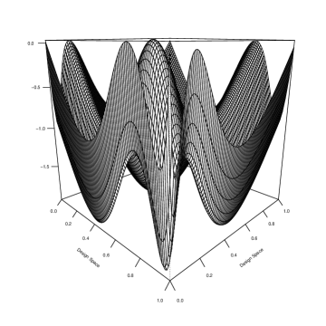
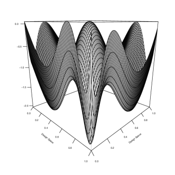
Figure 2: Illustration of Theorem 3.2. The figures show the function on left hand side of inequality (3.3). Left figure: The combination of exponential and EMAX model. Right figure: The combination of the loglinear and the exponential model.

Figure 3: Confidence bands obtained from the $\mu_{\infty}$-optimal design (solid lines) and a standard design (dashed lines). The dotted line shows the true difference of the curves. Left figure: The combination of exponential and EMAX model. Right figure: The combination of the loglinear and the exponential model.

In Figure 2 we demonstrate the application of the equivalence Theorem 3.2 for the combinations EMAX and exponential model and exponential and loglinear model. Figure 3 presents the improvement of the confidence bands for the difference between the two regression functions if the $\mu_{\infty}$-optimal design is used instead of a pair of the standard designs. The sample sizes in both groups are $n_{1}=100$ and $n_{2}=100$, respectively. The presented confidence bands are the averages of uniform confidence bands calculated by $100$ simulation runs. We observe that inference on the basis of an $\mu_{\infty}$-optimal design yields a substantial reduction in the (maximal) width of the confidence band.

model 1 / model 2	loglin / exp	loglin / EMAX	exp / EMAX
standard design	58.85	72.83	59.00
$D$-optimal designs for EMAX	2.21	93.81	2.24
$D$-optimal designs for loglinear	7.31	92.44	7.40
$D$-optimal designs for exponential	15.08	3.72	4.29
$\nu_{\infty}$-optimal design (model 1 fixed)	95.72	99.94	96.70
$\nu_{\infty}$-optimal design (model 2 fixed)	96.63	99.96	96.00

Table 3: The $\mu_{\infty}$-efficiencies (in $\%$) of the standard design, pairs of $D$-optimal designs (displayed in the diagonal blocks of Table 2) and the $\nu_{\infty}$-optimal designs (see Table 4) .

Besides the comparison of the different confidence bands produced by the $\mu_{\infty}$-optimal design and the standard design proposed in bretz2005 we are able to compare them using the efficiency defined by (3.4). The resulting efficiencies are depicted in the first row of Table 3. We observe a substantial loss of efficiency if the standard design is used instead of a $\mu_{\infty}$-optimal design. As described in the previous paragraph the $\mu_{\infty}$-optimal design is a pair of two identical $D$-optimal designs if both models coincide. These designs are depicted in the diagonal blocks of Table 2. In the row $2$-$4$ of Table 3 we show the corresponding efficiencies, if these designs are used for the comparison of curves. For example, the $\mu_{\infty}$-optimal design for two EMAX models has $\mu_{\infty}$-efficiencies $2.21\%$, $93.81\%$ and $2.24\%$, if it is used for the comparison of the loglinear and exponential, the loglinear and EMAX and the exponential and EMAX model, respectively. Note that the pair of $D$-optimal designs for the EMAX or loglinear model is more efficient than the standard designs, if these two models are under consideration. In all other cases these designs have very low efficiency and cannot be recommended for the comparison of curves. Finally, we consider the $\nu_{\infty}$-criterion defined in (2.6) assuming that the design for one model is already fixed as the $D$-optimal design and we calculate the corresponding $\nu_{\infty}$-optimal designs, which are depicted in Table 4 for the six possible combinations. For example, the $\nu_{\infty}$-optimal design for the comparison of the exponential and EMAX model where the design for the exponential model is fixed as $D$-optimal design puts weights $35.1\%$, $29.7\%$ and $35.2\%$ at the points $0.00$, $0.14$ and $1.00$, respectively. The $\mu_{\infty}$-efficiencies of these designs are presented in the row $5-6$ of Table 3 and we observe that these designs have very good efficiencies for the comparison of curves.

$m_{1}$/ $m_{2}$	EMAX			loglinear			exponential
EMAX	0.00	0.14	1.00	0.00	0.15	1.00	0.00	0.14	1.00
	$33.\bar{3}$	$33.\bar{3}$	$33.\bar{3}$	34.0	32.0	34.0	35.1	29.7	35.2
loglinear	0.00	0.23	1.00	0.00	0.23	1.00	0.00	0.22	1.00
	34.0	32.0	34.0	$33.\bar{3}$	$33.\bar{3}$	$33.\bar{3}$	36.0	28.0	36.0
exponential	0.00	0.76	1.00	0.00	0.75	1.00	0.00	0.75	1.00
	35.7	28.6	35.7	36.7	26.6	36.7	$33.\bar{3}$	$33.\bar{3}$	$33.\bar{3}$

Table 4: $\nu_{\infty}$-optimal designs, where one design is given by the $D$-optimal design of the second model. The weights are given in percent ($\%$).

6 Optimal allocation to the two groups

So far we have assumed that the sample sizes $n_{1}$ and $n_{2}$ in the two groups are fixed and cannot be chosen by the experimenter. In this section we will briefly indicate some results, if optimization can also be performed with respect to the relative proportions $\gamma_{1}=n_{1}/(n_{1}+n_{2})$ and $\gamma_{2}=n_{2}/(n_{1}+n_{2})$ for the two groups. Following the approximate design approach we define $\gamma$ as a probability measure with masses $\gamma_{1}$ and $\gamma_{2}$ at the points $0$ and $1$, respectively, and a $\mu_{\infty}$-optimal design as a triple $\xi^{\star,\infty}=(\xi^{\star,\infty}_{1},\xi^{\star,\infty}_{2},\gamma^{\star})$, which minimizes the functional

$$\mu_{\infty}(\xi_{1},\xi_{2},\gamma) = \sup_{t\in\mathcal{Z}}\varphi(t,\xi_{1},\xi_{2},\gamma),$$

where

$$\varphi(t,\xi_{1},\xi_{2},\gamma) = \frac{\sigma^{2}_{1}}{\gamma_{1}}f_{1}^{T}(t)M_{1}^{-1}(\xi_{1},\vartheta_{1})f_{1}(t)+\frac{\sigma^{2}_{1}}{\gamma_{2}}f_{2}^{T}(t)M_{2}^{-1}(\xi_{2},\vartheta_{2})f_{2}(t).$$

Similar arguments as given in the proof of Theorem 3.1 give a characterization of the optimal designs. The details are omitted for the sake of brevity.

Theorem 6.1.

A design $\xi^{\star,\infty}=(\xi^{\star,\infty}_{1},\xi^{\star,\infty}_{2},\gamma^{\star})$ is $\mu_{\infty}$-optimal if and only if there exists a measure $\varrho^{\star}$ on the set

$$\mathcal{Z}(\xi^{\star,\infty}_{1},\xi^{\star,\infty}_{2},\gamma^{\star})=\{t\in\mathcal{Z}:\mu_{\infty}(\xi^{\star,\infty}_{1},\xi^{\star,\infty}_{2},\gamma^{\star})=\varphi(t,\xi^{\star,\infty}_{1},\xi^{\star,\infty}_{2},\gamma^{\star})\}$$

such that the inequality

$$\int_{\mathcal{Z}(\xi^{\star,\infty}_{1},\xi^{\star,\infty}_{2},\gamma^{\star})}\tfrac{I\{\omega=0\}}{{\sigma_{1}^{2}}}\varphi_{1}^{2}(t,t_{1},\xi_{1}^{\star,\infty})+\tfrac{I\{\omega=1\}}{{\sigma_{2}^{2}}}\varphi_{2}^{2}(t,t_{2},\xi_{2}^{\star,\infty})\,d\varrho^{\star}(t)-\mu_{\infty}(\xi^{\star,\infty}_{1},\xi^{\star,\infty}_{2},\gamma^{\star})\leq 0\\$$ (5.2)

is satisfied for all $t_{1},t_{2}\in\mathcal{X}$ and $\omega\in\{0,1\}$, where $\varphi_{i}$ is defined in (3.2) with $\gamma_{i}=\gamma^{\star}_{i}$. Moreover, equality is achieved in (3.3) for any $(t_{1},t_{2},\omega)\in\mbox{supp}(\xi^{\star,\infty}_{1})\times\mbox{supp}(\xi^{\star,\infty}_{2})\times\{0,1\}$.

Example 6.2.

The $\mu_{\infty}$-optimal design $(\xi^{\star,\infty}_{1},\xi^{\star,\infty}_{2},\gamma^{\star})$ can be determined numerically in a similar way as described in Section 5, and we briefly illustrate some results for the comparison of the EMAX model with the exponential model, where the parameters are given in Table 1. The variances are $\sigma^{2}_{1}=1.478^{2}$ in the first group and $\sigma_{2}^{2}=5\cdot 1.478^{2}$ in the second group and the optimal designs (calculated by the PSO) are presented in Table 5. Note that the optimal design allocates only $30.2\%$ of the observations to the first group. A comparison of the optimal designs from Table 5 with the corresponding optimal designs from Table 2 (calculated under the assumptions $\sigma^{2}_{1}=\sigma^{2}_{2}$ and $\gamma_{1}=\gamma_{2}=0.5$) shows that the support points are very similar, but there appear differences in the weights.

$\gamma^{*}$	$\xi^{\star,\infty}_{1}$	$\xi^{\star,\infty}_{2}$
(30.2, 69.8)	$\begin{matrix}0.00&0.15&1.00\\ ~32.4&24.9&42.7\end{matrix}$	$\begin{matrix}0.00&0.75&1.00\\ ~36.9&30.4&32.7\end{matrix}$

Table 5: The $\mu_{\infty}$-optimal design $(\xi^{\star,\infty}_{1},\xi^{\star,\infty}_{2},\gamma^{\star})$ for the comparison of the EMAX- and exponential model, where optimization is also performed with respect to the relative sample sizes $\gamma=(\gamma_{1},\gamma_{2})$ for the two groups. The weights are given in $\%$.

Acknowledgements. The authors would like to thank Martina Stein, who typed parts of this manuscript with considerable technical expertise. We are also grateful to Kathrin Möllenhoff for interesting discussions on the subject of comparing curves and for computational assistance. This project has received funding from the European Union’s 7th Framework Programme for research, technological development and demonstration under the IDEAL Grant Agreement no 602552. The work has also been supported in part by the National Institute Of General Medical Sciences of the National Institutes of Health under Award Number R01GM107639. The content is solely the responsibility of the authors and does not necessarily represent the official views of the National Institutes of Health.

7 Proofs

Let $\Xi$ denote the space of all approximate designs on $\mathcal{X}$ and define for $\xi_{1},\xi_{2}\in\Xi$

$$M(\xi_{1},\xi_{2},\vartheta_{1},\vartheta_{2})=\begin{pmatrix}\frac{\gamma_{1}}{\sigma^{2}_{1}}M_{1}(\xi_{1},\vartheta_{1})&0_{s_{1}\times s_{2}}\\ 0_{s_{2}\times s_{1}}&\frac{\gamma_{2}}{\sigma^{2}_{2}}M_{2}(\xi_{2},\vartheta_{2})\end{pmatrix}$$ (7.1)

as the block diagonal matrix with information matrices $\frac{\gamma_{1}}{\sigma^{2}_{1}}M_{1}(\xi_{1},\vartheta_{1})$ and $\frac{\gamma_{2}}{\sigma^{2}_{2}}M_{2}(\xi_{2},\vartheta_{2})$ in the diagonal. The set

$$\mathcal{M}^{(2)}=\left\{M(\xi_{1},\xi_{2},\vartheta_{1},\vartheta_{2}):\xi_{1},\xi_{2}\in\Xi\right\}$$

is obviously a convex subset of the the set $\mbox{NND}(s_{1}+s_{2})$ of all non-negative definite $(s_{1}+s_{2})\times(s_{1}+s_{2})$ matrices. Moreover, if $\delta_{t}$ denotes the Dirac measure at the point $t\in{\cal X}$ it is easy to see that $\mathcal{M}^{(2)}$ is the convex hull of the set

$$\mathcal{D}^{(2)}=\left\{M(\delta_{t_{1}},\delta_{t_{2}},\vartheta_{1},\vartheta_{2}):t_{1},t_{2}\in\mathcal{X}\right\},$$

and that for any $p\in[1,\infty]$ the function $\mu_{p}(\xi)=\mu_{p}((\xi_{1},\xi_{2}))$ defined in (2.5) and (2) is convex on the set $\Xi\times\Xi$.

Proof of Theorem 3.1 Note that the function $\varphi$ in (2.2) can be written as

$$\varphi(t,\xi_{1},\xi_{2})=f^{T}(t)M^{-1}(\xi_{1},\xi_{2},\vartheta_{1},\vartheta_{2})f(t),$$

where $f^{T}(t)=(f^{T}_{1}(t),f^{T}_{2}(t))$ and $M(\xi_{1},\xi_{2})\in\mathcal{M}^{(2)}$ is defined in (7.1). Similarly, we introduce for a matrix $M\in\mathcal{M}^{(2)}$ the notation $\Phi(M,t)=f^{T}(t)M^{-1}f(t)$ and we rewrite the function $\mu_{p}(\xi_{1},\xi_{2})$ as

$$\tilde{\mu}_{p}(M)=\Bigl{(}\int_{\mathcal{Z}}\left(\Phi(M,t)\right)^{p}d\lambda(t)\Bigr{)}^{1/p}=\Bigl{(}\int_{\mathcal{Z}}\left(f^{T}(t)M^{-1}f(t)\right)^{p}d\lambda(t)\Bigr{)}^{1/p}.$$ (7.2)

Because of the convexity of $\mu_{p}$ the design $\xi^{\star,p}=(\xi_{1}^{\star,p},\xi_{2}^{\star,p})$ is $\mu_{p}$-optimal if and only if the derivative of $\tilde{\mu}_{p}(M)$ evaluated in $M_{0}=M(\xi_{1}^{\star,p},\xi_{2}^{\star,p},\vartheta_{1},\vartheta_{2})$ is non-negative for all directions $E_{0}=E-M_{0}$, where $E\in\mathcal{M}^{(2)}$, i.e. $\partial\tilde{\mu}_{p}(M_{0},E_{0})\geq 0.$ Since $\mathcal{M}^{(2)}=\mbox{conv}(\mathcal{D}^{(2)})$ it is sufficient to verify this inequality for all $E\in\mathcal{D}^{(2)}$.
Assuming that integration and differentiation are interchangeable, the derivative at $M_{0}=M(\xi_{1},\xi_{2},\vartheta_{1},\vartheta_{2})$ in direction $E_{0}=M(\delta_{t_{1}}\delta_{t_{2}},\vartheta_{1},\vartheta_{2})-M_{0}$ is given by

$$\partial\tilde{\mu}_{p}(M_{0},E_{0})=\tilde{\mu}_{p}(M_{0})^{1-p}\int_{\mathcal{Z}}\left(f^{T}(t)M_{0}^{-1}f(t)\right)^{p-1}\left(-f^{T}(t)M_{0}^{-1}E_{0}M^{-1}f(t)\right)d\lambda(t)$$

$$~{}~{}~{}=\tilde{\mu}_{p}(M_{0})^{1-p}\int_{\mathcal{Z}}\left(f^{T}(t)M_{0}^{-1}f(t)\right)^{p}d\lambda(t)$$

$$~{}~{}~{}\quad-\tilde{\mu}_{p}(M_{0})^{1-p}\int_{\mathcal{Z}}\left(f^{T}(t)M^{-1}f(t)\right)^{p-1}\left(f^{T}(t)M_{0}^{-1}M(\delta_{t_{1}},\delta_{t_{2}},\vartheta_{1},\vartheta_{2})M_{0}^{-1}f(t)\right)d\lambda(t)$$

$$~{}~{}~{}=\tilde{\mu}_{p}(M_{0})-\tilde{\mu}_{p}(M_{0})^{1-p}$$

$$~{}~{}~{}\int_{\mathcal{Z}}\Phi(M_{0},t)^{p-1}\Bigl{(}\tfrac{\sigma^{2}_{1}}{\gamma_{1}}(f^{T}_{1}(t)M_{1}^{-1}(\xi_{1},\vartheta_{1})f_{2}(t_{1}))^{2}+\tfrac{\sigma^{2}_{2}}{\gamma_{2}}(f^{T}_{2}(t)M_{2}^{-1}(\xi_{2},\vartheta_{2})f_{2}(t_{2}))^{2}\bigr{)}d\lambda(t)$$

$$~{}~{}~{}=\mu_{p}(\xi_{1},\xi_{2})\Bigl{[}1-{\mu}_{p}(\xi_{1},\xi_{2})^{-p}\int_{\mathcal{Z}}\beta(t,t_{1},t_{2})d\lambda(t)\Bigr{]},~{}~{}~{}~{}~{}~{}~{}~{}$$ (7.3)

where the function $\beta$ is given by

$$\beta(t,t_{1},t_{2})=\varphi(t,\xi_{1},\xi_{2})^{p-1}(\tfrac{\gamma_{1}}{\sigma^{2}_{1}}({\varphi}_{1}(t,t_{1},\xi_{1}))^{2}+\tfrac{\gamma_{2}}{\sigma^{2}_{2}}({\varphi}_{2}(t,t_{2},\xi_{2}))^{2}).$$ (7.4)

Consequently, the design $\xi^{\star,p}=(\xi^{\star,p}_{1},\xi^{\star,p}_{2})$ is $\mu_{p}$-optimal if and only if the inequality

$$\int_{\mathcal{Z}}\beta(t,t_{1},t_{2})d\lambda(t)-\left(\mu_{p}(\xi^{\star,p}_{1},\xi^{\star,p}_{2})\right)^{p}\leq 0$$ (7.5)

is satisfied for all $t_{1},t_{2}\in\mathcal{X}$, which proves the first part of the assertion.
It remains to prove that equality holds for any point $(t_{1},t_{2})\in\mbox{supp}(\xi^{\star,p}_{1})\times\mbox{supp}(\xi^{\star,p}_{2})$. For this purpose we assume the opposite, i.e. there exists a point $(t_{1},t_{2})\in\mbox{supp}(\xi^{\star,p}_{1})\times\mbox{supp}(\xi^{\star,p}_{2})$, such that there is strict inequality in (7.5). This gives

$$\int_{\mathcal{X}}\int_{\mathcal{X}}\int_{\mathcal{Z}}\beta(t,t_{1},t_{2})d\lambda(t)d\xi^{\star,p}_{1}(t_{1})d\xi^{\star,p}_{2}(t_{2})\\ <\left(\mu_{p}(\xi^{\star,p}_{1},\xi^{\star,p}_{2})\right)^{p}.$$

On the other hand, we have

$$\int_{\mathcal{X}}\int_{\mathcal{X}}\int_{\mathcal{Z}}\beta(t,t_{1},t_{2})d\lambda(t)d\xi^{\star,p}_{1}(t_{1})d\xi^{\star,p}_{2}(t_{2})=\int_{\mathcal{Z}}\varphi(t,\xi^{\star,p}_{1},\xi^{\star,p}_{2})^{p}d\lambda(t)=\left(\mu_{p}(\xi^{\star,p}_{1},\xi^{\star,p}_{2})\right)^{p}.$$

This contradiction shows that equality in (7.5) must hold whenever $(t_{1},t_{2})\in\mbox{supp}(\xi^{\star,p}_{1})\times\mbox{supp}(\xi^{\star,p}_{2})$.

Proof of Theorem 3.2 By the discussion at the beginning of the proof of Theroem 3.1 the minimization of the function $\mu_{\infty}(\xi_{1},\xi_{2})$ is equivalent to the minimization of

$$\tilde{\mu}_{\infty}(M)=\sup_{t\in\mathcal{Z}}\Phi(M,t)=\sup_{t\in\mathcal{Z}}f^{T}(t)M^{-1}f(t)$$ (7.6)

for $M\in\mathcal{M}^{(2)}$. From Theorem 3.5 in pshe1971 the subgradient of $\tilde{\mu}_{\infty}(M)$ evaluated at a matrix $M_{0}$ in direction $E$ is given by

$$\mbox{D}\tilde{\mu}_{\infty}(M_{0},E)=\Bigl{\{}\int_{\mathcal{Z}(M_{0})}\partial\Phi(M_{0},E,t)d\varrho(t):\varrho\mbox{ measure on }\mathcal{Z}(M_{0})\Bigr{\}},$$

where the set $\mathcal{Z}(M_{0})$ is defined by $\mathcal{Z}(M_{0})=\left\{t\in\mathcal{Z}:\tilde{\mu}_{\infty}(M_{0})=\Phi(M_{0},t)\right\},$ and the derivative of $\Phi(M_{0},t)$ in direction $E$ is given by $\partial\Phi(M_{0},E,t)=-f^{T}(t)M_{0}^{-1}EM_{0}^{-1}f(t).$ Applying the results from page $59$ in pshe1971 it therefore follows that the design $\xi^{\star,\infty}=(\xi^{\star,\infty}_{1},\xi^{\star,\infty}_{2})$ is $\mu_{\infty}$-optimal if and only if there exists a measure $\varrho^{\star}$ on $\mathcal{Z}(M(\xi^{\star,\infty}_{1},\xi^{\star,\infty}_{2},\vartheta_{1},\vartheta_{2}))$ such that the inequality

$$\int_{\mathcal{Z}(M_{0})}\partial\Phi(M_{0},E_{0},t)d\varrho^{\star}(t)=\int_{\mathcal{Z}(M_{0})}\partial\Phi(M_{0},E,t)d\varrho^{\star}(t)+\int_{\mathcal{Z}(M_{0})}f^{T}(t)M_{0}^{-1}f(t)d\varrho^{\star}(t)\geq 0$$

holds for all $E_{0}=E-M_{0}$, $E\in\mathcal{M}^{(2)}$. Since $\mathcal{M}^{(2)}=\mbox{conv}(\mathcal{D}^{(2)})$ it is sufficient to consider the directions $E_{0}=E-M_{0}$, where $E\in\mathcal{D}^{(2)}$. Thus, this inequality is fulfilled if and only if there exists a measure $\varrho^{\star}$ on $\mathcal{Z}(M_{0})=\mathcal{Z}(\xi^{\star,\infty})$, such that the inequality

$$\begin{split}\int_{\mathcal{Z}(\xi^{\star,\infty})}&f^{T}(t)M^{-1}(\xi^{\star,\infty}_{1},\xi^{\star,\infty}_{2},\vartheta_{1},\vartheta_{2})M(\delta_{t_{1}},\delta_{t_{2}},\vartheta_{1},\vartheta_{2})M^{-1}(\xi^{\star,\infty}_{1},\xi^{\star,\infty}_{2},\vartheta_{1},\vartheta_{2})d\varrho^{\star}(t)\\ \leq&\int_{\mathcal{Z}(\xi^{\star,\infty})}f^{T}(t)M^{-1}(\xi^{\star,\infty}_{1},\xi^{\star,\infty}_{2},\vartheta_{1},\vartheta_{2})f(t)\,d\varrho^{\star}(t)=\mu_{\infty}(\xi^{\star,\infty}_{1},\xi^{\star,\infty}_{2})\end{split}$$ (7.7)

is satisfied for all $M(\delta_{t_{1}},\delta_{t_{2}},\vartheta_{1},\vartheta_{2})\in\mathcal{D}^{(2)}$. Observing the definition of $\varphi_{i}$ in (3.2), the left-hand part of (7.7) can be rewritten as $\int_{\mathcal{Z}(\xi^{\star,\infty})}\tfrac{\gamma_{1}}{\sigma^{2}_{1}}{\varphi}^{2}_{1}(t_{1},t,\xi^{\star,\infty}_{1})+\tfrac{\gamma_{2}}{\sigma^{2}_{2}}{\varphi}^{2}_{2}(t_{2},t,\xi^{\star,\infty}_{2})\,d\varrho^{\star}(t),$ and the inequality (7.7) reduces to (3.3). The remaining statement regarding the equality at the support points follows by the same arguments as in the proof of Theorem 3.1 and the details are omitted for the sake of brevity.

Proof of Theorem 3.3 For both cases consider the function $(\tilde{\mu}_{p}(M))^{-1}$ where $\tilde{\mu}_{p}$ has already been defined in (7.2) and (7.6). Note that for each $t\in\mathcal{Z}$ the function $M\to(f(t)^{T}M^{-1}f(t))^{-1}$ is concave [see pukelsheim2006, p. 77], and consequently the function

$$(\tilde{\mu}_{\infty}(M))^{-1}={1\over\max_{t\in\mathcal{Z}}f(t)^{T}M^{-1}f(t)}=\min_{t\in\mathcal{Z}}(f(t)^{T}M^{-1}f(t))^{-1}$$

is also conave. The concavity of $(\tilde{\mu}_{p}(M))^{-1}$ in the case $1\leq p<\infty$ follows by similar arguments. For $p\in[1,\infty]$ the directional derivative of $(\tilde{\mu}_{p}(M))^{-1}$ at the point $M_{0}$ in direction $E_{0}=M-M_{0}$ is given by

$$\partial{(\tilde{\mu}_{p}}(M_{0},E_{0}))^{-1}=-(\tilde{\mu}_{p}(M_{0}))^{-2}\partial{\tilde{\mu}_{p}}(M_{0},E_{0}).$$

We now consider the case $p\in[1,\infty)$, the remaining case $p=\infty$ is briefly indicated at the end of this proof. Observing (7.3) a lower bound of the directional derivative of ${\tilde{\mu}_{p}}$ at $M_{0}=M(\xi_{1},\xi_{2},\vartheta_{1},\vartheta_{2})$ in direction $E_{0}=M(\delta_{t_{1}}\delta_{t_{2}},\vartheta_{1},\vartheta_{2})-M_{0}$ is given by

$$\partial{\tilde{\mu}_{p}}(M_{0},E_{0}) \geq \tilde{\mu}_{p}(M_{0})\Bigl{[}1-{\max_{t_{1},t_{2}}\int_{\mathcal{Z}}\beta(t,t_{1},t_{2})d\lambda(t)\over{\tilde{\mu}}_{p}^{p}(M_{0})}\Bigr{]}$$

where $\beta(t,t_{1},t_{2})$ is defined in (7.4). Consequently, we have

$$\partial{(\tilde{\mu}_{p}}(M_{0},E_{0}))^{-1}\leq\frac{1}{\tilde{\mu}_{p}(M_{0})}\Bigl{[}{\max_{t_{1},t_{2}}\int_{\mathcal{Z}}\beta(t,t_{1},t_{2})d\lambda(t)\over{\tilde{\mu}}_{p}^{p}(M_{0})}-1\Bigr{]}.$$ (7.8)

Now, we consider the matrices $M_{0}=M(\xi_{1}^{\star,p},\xi_{2}^{\star,p},\vartheta_{1},\vartheta_{2})$ of the $\mu_{p}$-optimal design and $M=M(\xi_{1},\xi_{2},\vartheta_{1},\vartheta_{2})$ of any design $\xi=(\xi_{1},\xi_{2})$ with nonsingular information matrices $M_{1}(\xi_{1},\vartheta_{1})$ and $M_{2}(\xi_{2},\vartheta_{2})$ and define the function $g_{p}(\alpha)=\tilde{\mu}_{p}((1-\alpha)M_{0}+\alpha M))^{-1}$, which is concave because of the concavity of $(\tilde{\mu}_{p}(M))^{-1}$. This yields

$$\frac{1}{\tilde{\mu}_{p}(M)}-\frac{1}{\tilde{\mu}_{p}(M_{0})} = g_{p}(1)-g_{p}(0)\leq{\partial g_{p}(\alpha)\over\partial\alpha}\Bigl{|}_{\alpha=0}=\partial{(\tilde{\mu}_{p}}(M_{0},E_{0}))^{-1}$$

Consequently, we obtain from (7.8) the inequality

$$\mbox{eff}_{p}(\xi)=\frac{\tilde{\mu}_{p}(M)}{\tilde{\mu}_{p}(M_{0})}\geq\frac{\tilde{\mu}^{p}_{p}(M)}{\max_{t_{1},t_{2}}\int_{\mathcal{Z}}\beta(t,t_{1},t_{2})d\lambda(t)},$$

which proves the assertion of Theorem 3.3 in the case $1\leq p<\infty$. For the proof in the case $p=\infty$ we use similar arguments and Theorem 3.2 in pshe1971, which provides the upper bound

$$\partial{(\tilde{\mu}_{\infty}(M_{0},E_{0}))^{-1}}\leq\frac{1}{\tilde{\mu}_{\infty}(M_{0})}\Bigl{\{}\max_{d\in\mathcal{Z}(M_{0})}\max_{t_{1},t_{2}\in\mathcal{X}}(f^{T}(d)M^{-1}_{0}f(t_{1},t_{2}))^{2}-1\Bigr{\}},$$ (7.9)

where $f(t_{1},t_{2})$ is defined by $f^{T}(t_{1},t_{2})=(f_{1}^{T}(t_{1}),f^{T}_{2}(t_{2}))^{T}$. The details are omitted for the sake of brevity.

Proof of Theorem 4.1 For the sake of brevity we now restrict ourselves to the proof of the first part of Theorem 4.1. The second part can be proved analogously. Let $U_{\mathcal{X}}<L_{\mathcal{Z}}$ and recall the definition of the function $\varphi(t,\xi_{1},\xi_{2})$ defined in (2.2). The function $\varphi(t,\xi_{1},\xi_{2})$ is obviously increasing on $\mathcal{Z}$, if the functions

$$\varphi_{i}(t,t,\xi_{i})={\sigma_{i}^{2}\over\gamma_{i}}f^{T}_{i}(t)M_{i}^{-1}(\xi_{i})f_{i}(t)={\sigma_{i}^{2}\over\gamma_{i}}\omega_{i}^{2}(t)(1,t,\ldots,t^{p_{i}})M^{-1}_{i}(\xi_{i})(1,t,\ldots,t^{p_{i}})^{T}$$

are increasing on $\mathcal{Z}$ for $i=1,2$. In this case we have

$$\max_{t\in\mathcal{Z}}\varphi(t,\xi_{1},\xi_{2})=\varphi(U_{\mathcal{Z}},\xi_{1},\xi_{2})=\varphi_{1}(U_{\mathcal{Z}},\xi_{1})+\varphi_{2}(U_{\mathcal{Z}},\xi_{2}).$$ (7.10)

Because of this structure the components of the optimal design can be calculated separately for $\varphi_{1}$ and $\varphi_{2}$. Since both $\{\omega_{1}(t),\omega_{1}(t)t,\ldots,\omega_{1}(t)t^{p_{1}}\}$ and $\{\omega_{2}(t),\omega_{2}(t)t,\ldots,\omega_{2}(t)t^{p_{2}}\}$ are Chebyshev systems on $\mathcal{X}\cup\mathcal{Z}$ it follows from Theorem X.7.7 in karstu1966 that the support points of the design $\xi_{i}$ minimizing $\varphi_{i}(U_{\mathcal{Z}},\xi_{i})$ are given by the extremal points of the equioscillating polynomials $\underline{v}_{i}(t)$, while the corresponding weights are given by (4.2).
In order to prove the monotonicity of $\varphi_{i}$, ($i=1,2$) let $\xi_{i}$ denote a design with $k_{i}$ support points $t_{i0},\ldots,t_{i{k_{i}-1}}\in\mathcal{X}$ and corresponding weights $\xi_{i0},\ldots,\xi_{i{k_{i}-1}}$.
Since$\{1,\omega_{i}(t),\omega_{i}(t)t,\ldots,\omega_{i}(t)t^{2p_{i}-1}\}$ and $\{1,\omega_{i}(t),\omega_{i}(t)t,\ldots,\omega_{i}(t)t^{2p_{i}}\}$ are Chebshev systems for $\omega_{i}(t)\neq c\in\mathbb{R}$, the complete class theorem of detmel2011 can be applied and it is sufficient to consider minimal supported designs $\xi_{i}$. Consequently, we set $k_{i}=p_{i}+1$.

Define $X_{i}=\left(\omega_{i}(t_{ik})t^{l}_{ik}\right)_{k,l=0,\ldots,p_{i}}$, then it is easy to see that the $j$th Langrange interpolation polynomial is given by $L_{ij}(t)=e_{j}^{T}X_{i}^{-1}\left(\omega_{i}(t),\omega_{i}(t)t,\ldots,\omega_{i}(t)t^{p_{i}}\right)^{T}$, where $e_{j}$ denotes the $j$th unit vector (just check the defining condition $L_{ij}(t_{i\ell})=\delta_{j\ell}$). With these notations the function $\varphi_{i}(t,\xi_{i})$ can be rewritten as

$$\begin{split}\varphi_{i}(t,t,\xi_{i})&={\sigma_{i}^{2}\over\gamma_{i}}\left(\omega_{i}(t),\omega_{i}(t)t,\ldots,\omega_{i}(t)t^{p_{i}}\right)X_{i}^{-T}W^{-1}_{i}X_{i}^{-1}\left(\omega_{i}(t),\omega_{i}(t)t,\ldots,\omega_{i}(t)t^{p_{i}}\right)^{T}\\ &:={\sigma_{i}^{2}\over\gamma_{i}}\sum_{j=0}^{p_{i}}\frac{1}{\xi_{ij}}(L_{ij}(t))^{2},\end{split}$$ (7.11)

where $W_{i}=\mbox{diag}(\xi_{i0},\ldots,\xi_{ip_{i}})$. Now Cramer’s rule and a straightforward calculation yields the following representation for the Lagrange interpolation polynomial

$$L_{ij}(t) = (-1)^{p_{i}-j}\omega_{i}(t)\frac{\prod_{k=0,k\neq j}^{p_{i}}\omega_{i}(t_{ik})}{\prod_{k=0}^{p_{i}}\omega_{i}(t_{ik})}\frac{\det\begin{pmatrix}1&\ldots&1&1&\ldots&1&1\\ t_{i0}&\ldots&t_{ij-1}&t_{ij+1}&\ldots&t_{ip_{i}}&t\\ \vdots&\ldots&\vdots&\vdots&\ldots&\vdots&\vdots\\ t^{p_{i}}_{i0}&\ldots&t^{p_{i}}_{ij-1}&t^{p_{i}}_{ij+1}&\ldots&t^{p_{i}}_{ip_{i}}&t^{p_{i}}\end{pmatrix}}{\det\begin{pmatrix}1&\ldots&1\\ t_{i0}&\ldots&t_{ip_{i}}\\ \vdots&\ldots&\vdots\\ t^{p_{i}}_{i0}&\ldots&t^{p_{i}}_{ip_{i}}\end{pmatrix}}$$

$$= \frac{\omega_{i}(t)}{\omega_{i}(t_{j})}\prod_{k=0,k\neq j}^{p_{i}}\frac{t-t_{ik}}{t_{ij}-t_{ik}}.$$

Therefore the partial derivative of $\varphi_{i}(t,\xi_{i})$ with respect to $t$ is given by

$$\frac{\partial}{\partial t}\varphi_{i}(t,t,\xi_{i})={\sigma_{i}^{2}\over\gamma_{i}}\sum_{j=0}^{p_{i}}\frac{2}{\xi_{ij}}(L_{ij}(t))^{2}\Bigl{(}\frac{\omega^{\prime}_{i}(t)}{\omega_{i}(t)}+\sum_{l=0}^{p_{i}}\frac{1}{t-t_{il}}\Bigr{)}.$$

Note that $t_{il}<t$ for all $t_{il}\in\mathcal{X}$ and $t\in\mathcal{Z}$ and that both $\omega_{i}(t)$ and $\omega^{\prime}_{i}(t)$ are positive. Consequently, the partial derivative is positive and the function $\varphi_{i}(t,\xi_{i})$ is increasing in $t\in\mathcal{Z}$. Thus, the maximum value of $\varphi_{i}(t,\xi_{i})$ is attained in $U_{\mathcal{Z}}\in\mathcal{Z}$ and (7.10) follows.

Proof of Corollary 4.3 For the sake of brevity we only prove the result for the EMAX model (4.6), where it essentially follows by an application of Theorem 4.1 with $\omega(t)\equiv 1$. The proofs for the Michaelis Menten model and for the loglinear model are similar. In the the EMAX model the gradient is given by $f(t,\vartheta)=(1,\frac{t}{t+\vartheta_{3}},\frac{-\vartheta_{2}t}{(t+\vartheta_{3})^{2}})$. Using the strictly increasing transformation $z=v(t)=\frac{t}{\vartheta_{3}+t}$ the function $f$ can be rewritten by

$$f(t,\vartheta)=\begin{pmatrix}1&0&0\\ 0&1&0\\ 0&-\frac{\vartheta_{2}}{\vartheta_{3}}&\frac{\vartheta_{2}}{\vartheta_{3}}\end{pmatrix}\begin{pmatrix}1\\ z\\ z^{2}\end{pmatrix}:=P_{\vartheta}\begin{pmatrix}1\\ z\\ z^{2}\end{pmatrix}.$$

Thus, for an arbitrary design $\xi$ the function $f^{T}(t)M^{-1}(\xi)f(t)$ reduces to

$$\varphi(t,\xi)=f^{T}(t)M^{-1}(\xi)f(t) = (1,z,z^{2})P_{\vartheta}^{T}\left(P_{\vartheta}\tilde{M}(\tilde{\xi})P^{T}_{\vartheta}\right)^{-1}P_{\vartheta}\,(1,z,z^{2})^{T}$$

$$= (1,z,z^{2})\tilde{M}^{-1}(\tilde{\xi})(1,z,z^{2})^{T}=\tilde{\varphi}(z,\tilde{\xi})$$

where $\tilde{M}(\tilde{\xi})=(\int_{\mathcal{X}}z^{i+j}d\tilde{\xi}(z))_{i,j=0,1,2}$ and $\tilde{\xi}$ is the design on the design space $\tilde{\mathcal{X}}=[\frac{L_{\mathcal{X}}}{\vartheta_{3}+L_{\mathcal{X}}},\frac{U_{\mathcal{X}}}{\vartheta_{3}+U_{\mathcal{X}}}]$ induced from the actual design $\xi$ by the transformation $z=\frac{t}{\vartheta_{3}+t}$. The function $\tilde{\varphi}(z,\tilde{\xi})$ coincides with the variance function of a polynomial regression model with degree $2$ and constant weight function $\omega(t)\equiv 1$. The corresponding design and extrapolation space are given by $\tilde{\mathcal{X}}=[\frac{L_{\mathcal{X}}}{\vartheta_{3}+L_{\mathcal{X}}},\frac{U_{\mathcal{X}}}{\vartheta_{3}+U_{\mathcal{X}}}]$ and $\tilde{\mathcal{Z}}=[\frac{L_{\mathcal{Z}}}{\vartheta_{3}+L_{\mathcal{Z}}},\frac{U_{\mathcal{Z}}}{\vartheta_{3}+U_{\mathcal{Z}}}]$, respectively. According to Example 4.2 $(p_{1}=2)$ the component $\tilde{\xi}_{i}$ of the $\mu_{\infty}$-optimal design is supported at the extremal points of the Chebyshev polynomial of the first kind on the interval $\mathcal{X}$, which are given by

$$\frac{L_{\mathcal{X}}}{\vartheta_{3}+L_{\mathcal{X}}},~{}{1\over 2}\Bigl{(}\frac{L_{\mathcal{X}}}{\vartheta_{3}+L_{\mathcal{X}}}+\frac{U_{\mathcal{X}}}{\vartheta_{3}+U_{\mathcal{X}}}\Bigr{)},~{}\frac{U_{\mathcal{X}}}{\vartheta_{3}+U_{\mathcal{X}}}$$

For the weights we obtain by the same result $\xi_{0}=\tfrac{|L_{0}|}{L},\xi_{1}=\tfrac{|L_{1}|}{L},\xi_{2}=\tfrac{|L_{2}|}{L}$ where

$$|L_{0}| = \left(2\tfrac{U_{\mathcal{Z}}}{U_{\mathcal{Z}}+\vartheta_{3}}-\left(\tfrac{U_{\mathcal{X}}}{U_{\mathcal{X}}+\vartheta_{3}}+\tfrac{L_{\mathcal{X}}}{L_{\mathcal{X}}+\vartheta_{3}}\right)\right)\left(\tfrac{U_{\mathcal{Z}}}{U_{\mathcal{Z}}+\vartheta_{3}}-\tfrac{U_{\mathcal{X}}}{U_{\mathcal{X}}+\vartheta_{3}}\right)$$

$$|L_{1}| = 4\left(\tfrac{U_{\mathcal{Z}}}{U_{\mathcal{Z}}+\vartheta_{3}}-\tfrac{L_{\mathcal{X}}}{L_{\mathcal{X}}+\vartheta_{3}}\right)\left(\tfrac{U_{\mathcal{Z}}}{U_{\mathcal{Z}}+\vartheta_{3}}-\tfrac{U_{\mathcal{X}}}{U_{\mathcal{X}}+\vartheta_{3}}\right)$$

$$|L_{2}| = \left(\tfrac{U_{\mathcal{Z}}}{U_{\mathcal{Z}}+\vartheta_{3}}-\tfrac{L_{\mathcal{X}}}{L_{\mathcal{X}}+\vartheta_{3}}\right)\left(2\tfrac{U_{\mathcal{Z}}}{U_{\mathcal{Z}}+\vartheta_{3}}-\left(\tfrac{U_{\mathcal{X}}}{U_{\mathcal{X}}+\vartheta_{3}}+\tfrac{L_{\mathcal{X}}}{L_{\mathcal{X}}+\vartheta_{3}}\right)\right)$$

$$L = |L_{0}|+|L_{1}|+|L_{2}|.$$

The support points of the of the $\mu_{\infty}$-optimal design $\xi$ are now obtained by the inverse of the transformation and the assertion for the EMAX model follows from the definition of the function $g$ and a straightforward calculation.