On the semimetal-insulator transition and Lifshitz transition in simulations of mono-layer graphene

Abstract:

We report on the status of ongoing Hybrid-Monte-Carlo simulations of the tight-binding model of mono-layer graphene. We present results concerning the semimetal-insulator phase transition, whereby two-body interactions are modeled by a partially screened Coulomb potential which takes into account screening by electrons in the lower $\sigma$-orbitals. We obtain evidence that finite-size effects may still be present in the current estimate of the critical coupling strength $\alpha_{C}$, which was previously extracted from simulations on lattice-sizes up to $N_{x}=N_{y}=18$. We also present preliminary results concerning the Neck-disrupting Lifshitz transition which occurs at finite Fermion-density in the limit of vanishing two-body interactions. A sign-problem is circumvented by using a spin-dependent chemical potential in our simulations.

1 Introduction

In recent years, much interest has arisen in graphene, a two-dimensional sheet of carbon atoms arranged on a hexagonal lattice, due to its many unusual properties which make it an interesting candidate for a number of technological applications [1]. From a theoretical perspective, graphene is interesting because its electronic properties are governed by a massless Dirac equation in the limit of low energies and because the small Fermi velocity $v_{F}\approx c/300$ leads to strong electromagnetic interactions with an effective fine-structure constant of $\alpha_{\textrm{eff}}=e^{2}/(\hbar v_{F})\approx 2.2$ [2]. Thus, graphene provides an example of the physics of strongly coupled relativistic field theory, realized in a condensed matter system. Furthermore, the coupling-constant in graphene can be directly manipulated by affixing the sheet to a substrate, which leads to di-electric rescaling $\alpha_{\textrm{eff}}\to\alpha_{\textrm{eff}}/\epsilon$.

Early on, the lattice community took an interest in graphene since it seemed obvious that the well-developed machinery for simulating field theories should be applicable. Several works were published which focused on electronic properties in the low-energy limit (see e.g. Refs. [3]). Later it was shown how the full microscopic theory with hexagonal symmetry can be formulated as a lattice theory [4]. This was henceforth adopted as the de-facto standard and a number of works were published presenting simulations based on this derivation [5, 6, 7, 8].

In this work we report on our ongoing efforts to simulate the electronic properties of graphene via Hybrid-Monte-Carlo. We implement a fully hexagonal lattice theory based on the derivations presented in Ref. [4].

The aim of this paper is two-fold: After summarizing the methodology, we first present a follow-up discussion of our investigation of the semimetal-insulator phase-transition which was published in Ref. [8]. Therein simulations of the interacting tight-binding theory of graphene were presented in which electronic two-body interactions were modeled by a partially screened Coulomb potential, which accounts for screening by electrons in the lower $\sigma$-orbits at short distances and crosses over smoothly to an unscreened Coulomb potential at long distances. We contrasted these results to a similar study presented in Ref. [6], which instead assumed that at long distances the potential is screened by a constant di-electric screening factor. We found that for a lattice of dimensions $N_{x}=N_{y}=18$ the exact form of the long-range tail doesn’t seem to affect the precise location of the critical coupling strength $\alpha_{C}$ for gap-formation much. In this work we present results obtained on $N_{x}=N_{y}=36$ which may indicate that for larger systems the transition is shifted to smaller $\alpha_{C}$. This would mean that previous simulations are affected by finite-size effects and that an extrapolation to infinite surface area is in order to conclusively decide whether the long-range part of the potential is of relevance.

Second we present preliminary results concerning the Neck-disrupting Lifshitz transition, which is known to occur in the limit of vanishing two-body interactions at finite Fermion-density and which is characterized by a change of the topology of the Fermi surface and a logarithmic divergence of the density of states [9]. To avoid a Fermion sign-problem we implement the “isospin” chemical potential, the sign of which differs for the two spin-orientations of electrons. The results presented here concern the non-interacting limit only. Our long-term goal is to investigate how a small interaction term affects the Lifshitz transition.

2 The setup

The setup of our simulations has been described in great detail in Ref. [8], where a step-by-step derivation of every component of the Hybrid-Monte-Carlo algorithm for the interacting tight-binding theory based on the concepts worked out in Ref. [4] is presented. We will only summarize the basic principles here. Our goal is to simulate the thermodynamics of the interacting tight-binding theory of graphene

$$H=\sum_{\langle x,y\rangle}(-\kappa)(a_{x}^{\dagger}a_{y}-b_{x}^{\dagger}b_{y}+\textrm{h.c.})+\sum_{x,y}\,q_{x}V_{xy}q_{y}+\sum_{x}m_{s}(a_{x}^{\dagger}a_{x}+b_{x}^{\dagger}b_{x})~{},$$ (1)

where $a_{x},a_{x}^{\dagger},b_{x},b_{x}^{\dagger}$ are ladder operators for particles with spin $+1/2$ and anti-particles (“holes”) with spin $-1/2$ respectively. The sums run over all pairs of nearest neighbors, pairs of coordinates and all coordinates of the hexagonal lattice respectively. $q_{x}=a_{x}^{\dagger}a_{x}-b_{x}^{\dagger}b_{x}$ is the charge operator, $\kappa\approx 2.7$ the hopping parameter and $m_{s}$ a “staggered” mass-term, the sign of which alternates on the triangular sub-lattices of the hexagonal lattice. The mass term is added to remove zero-modes from the Hamiltonian and the limit $m_{s}\to 0$ is later taken. The matrix $V$, which describes two-body interactions, must be positive-definite but otherwise may be chosen arbitrarily. We use the “partially screened Coulomb potential” in our simulations as described below.

A lattice path-integral representation for the grand-canonical partition function $Z={\rm Tr}\,e^{-\beta H}$, in which the operators $a_{x},a_{x}^{\dagger},b_{x},b_{x}^{\dagger}$ are replaced by Grassmann-valued field variables, can be derived by factorizing $e^{-\beta H}$ into $N_{t}$ terms (implying a discretization error ${\cal O}(\delta^{2})$ where $\delta=\beta/N_{t}$) and inserting complete sets of of Fermionic coherent states. The interaction term $\sim q_{x}V_{xy}q_{y}$ at first prevents the usual procedure of integrating out Grassmann-fields via Gaussian integration, since it contains fourth-powers of latter operators. These can be eliminated through Hubbard-Stratonovich transformation

$$\exp\big{\{}-\frac{\delta}{2}\sum_{x,y}q_{x}V_{xy}q_{y}\big{\}}\propto\int\big{[}\prod_{x}\phi_{x}\big{]}\,\exp\big{\{}-\frac{\delta}{2}\sum_{x,y}\phi_{x}V_{xy}^{-1}\phi_{y}-i\,\delta\sum_{x}\phi_{x}q_{x}\big{\}}~{},$$ (2)

at the expense of introducing a dynamical scalar auxiliary field $\phi$ (“Hubbard field”), which plays the role of a gauge field. In fact, $\phi$ can be understood as representing the scalar electric potential. A magnetic vector-potential does not appear since interactions are taken to be instantaneous (which is a valid approximation since $v_{F}\ll c$). The final result is the functional integral

$$Z=\int\mathcal{D}\phi\,\det\big{[}M(\phi)M^{\dagger}(\phi)\big{]}\exp\big{\{}-\frac{\delta}{2}\sum_{t=0}^{N_{t}-1}\sum_{x,y}\phi_{x,t}V_{xy}^{-1}\phi_{y,t}\big{\}}~{},$$ (3)

which is of a form that can be dealt with, using a standard Hybrid-Monte-Carlo algorithm to generate representative configurations of the Hubbard field $\phi$. The Fermion-operator is given by

$$M_{(x,t)(y,t^{\prime})}~{}=~{}\delta_{xy}(\delta_{tt^{\prime}}-e^{-i\frac{\beta}{N_{t}}\phi_{x,t}}\delta_{t-1,t^{\prime}})-\kappa\frac{\beta}{N_{t}}\sum\limits_{\vec{n}}\delta_{y,x+\vec{n}}\delta_{t-1,t^{\prime}}+m_{s}\frac{\beta}{N_{t}}\delta_{xy}\delta_{t-1,t^{\prime}}~{}.$$ (4)

We choose to simulate rectangular graphene sheets with periodic boundary conditions. The dimensions $N_{x}$ and $N_{y}$ refer to the rhombic coordinate system which spans the triangular sub-lattices.

3 Semimetal-insulator transition

A question which is of immediate significance to technological applications (since electronic devices require a gate-voltage) is whether two-body interactions generate a band-gap for some effective coupling constant $\alpha_{\textrm{eff}}$ which is smaller than the upper bound given by suspended graphene ($\alpha_{\textrm{eff}}\approx 2.2$). This corresponds to electronic quasi-particles acquiring a dynamical mass and at a microscopic level implies a spontaneous breaking of the symmetry under exchange of the two triangular sub-lattices by formation of some condensate. Both charge-density-wave (CDW) and spin-density-wave (SDW) formation are mechanisms which have been discussed in literature. As a result of studies which directly assumed or indirectly implied that the two-body interactions in graphene were essentially unmodified Coulomb-type interactions (see e.g. Refs. [3, 5] and references therein) it was predicted that the transition to a gapped phase happens for $\alpha_{\textrm{eff}}\gtrsim 1.0$, well within the physically accessible region. This contradicted experiments which found graphene in vacuum to be a conductor [10].

In Ref. [6] a Monte-Carlo study of the formation of an anti-ferromagnetic condensate was conducted which suggested screening of interactions by electrons in the lower $\sigma$-orbitals as a mechanism which moves the transition to $\alpha_{\textrm{eff}}\approx 3.14$ (to the unphysical region) and thus reconciles theory with experiment. Therein explicit values for the on-site ($V_{00}$), nearest-neighbor ($V_{01}$), next-nearest-neighbor ($V_{02}$) and third-nearest-neighbor ($V_{03}$) potentials from calculations within a constrained random phase approximation (cRPA) conducted in Ref. [11] were used. At long distances, it was assumed that the potential falls off as $\sim 1/(\epsilon_{\sigma}\,r)$, where the constant $\epsilon_{\sigma}\approx 1.41$ was adjusted to match the $V_{03}$ term. A single lattice-size ($N_{x}=N_{y}=18,N_{t}=20$) and temperature ($\beta=2\mathrm{eV}^{-1}$) were considered.

Our work (Ref. [8]) aimed at eliminating residual doubts concerning the long range tail. At long-distances we thus instead used a phenomenological model

$$\epsilon^{-1}_{\sigma}(\vec{k})=\frac{1}{\epsilon_{1}}\frac{\epsilon_{1}+1+(\epsilon_{1}-1)e^{-kd}}{\epsilon_{1}+1-(\epsilon_{1}-1)e^{-kd}}~{},$$ (5)

proposed in Ref. [11] that describes a thin film of thickness $d=2.8\;\textrm{\AA}$ ($\approx 1.41\cdot 10^{-3}\,\mathrm{eV}^{-1}$) with a dielectric screening constant $\epsilon_{1}=2.4$ and computed a partially screened Coulomb potential via Fourier back-transformation

$$V(\vec{r}) =\frac{1}{(2\pi)^{2}}\int_{\mathbb{K}^{2}}d^{2}k\,\widetilde{V}_{0}(\vec{k})\,\epsilon^{-1}_{\sigma}(\vec{k})\,e^{-i\vec{k}\vec{r}}~{},\quad\quad\widetilde{V}_{0}(\vec{k})=(2\pi e^{2})/k~{},$$ (6)

which smoothly goes over to an unscreened potential as $r\to\infty$ (see Fig. 1, left). Simulations using this potential were carried out, and the $\alpha_{\textrm{eff}}$ dependence of the anti-ferromagnetic condensate

$$\Delta_{N}=\frac{1}{N_{x}N_{y}}\big{\{}\sum\limits_{x\in X_{A}}(a^{\dagger}_{x}a_{x}+b^{\dagger}_{x}b_{x})-\sum\limits_{x\in X_{B}}(a^{\dagger}_{x}a_{x}+b^{\dagger}_{x}b_{x})\big{\}},$$ (7)

was investigated for $N_{x}=N_{y}=18,N_{t}=20$ and $\beta=2\mathrm{eV}^{-1}$ (the sums in Eq. (7) run over coordinates in the two sub-lattices). We found no substantial difference to the results of Ref. [6] and thus concluded that the gap-transition is insensitive to the long-range tail of the potential for this lattice-size.

Fig. 1, right, shows recent results for $\Delta_{N}(\alpha_{\textrm{eff}})$ which were obtained on several hundreds of independent configurations of a $N_{x}=N_{y}=36,N_{t}=20$ lattice (for a range of $m_{s}$ which allowed the limit $m_{s}\to 0$ to be taken) and compares them with our published results obtained from $N_{x}=N_{y}=18$. A slight systematic effect is visible which may indicate a small shift of the transition to a smaller value of $\alpha_{\textrm{eff}}$. We take this result as evidence that finite-volume effects may still be present on $N_{x}=N_{y}=18$ and that an infinite volume extrapolation is thus in order. It is conceivable that the precise form of the long-range tail becomes more relevant for larger system-size.

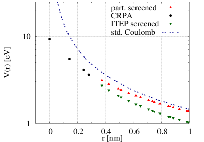
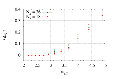
Figure 1: Left: Comparison of standard Coulomb potential, partially screened potential and potential used in Ref. [6] (“ITEP screened”). Right: Order-parameter for gap-transition in the limit $m_{s}\to 0$.

4 Neck-disrupting Lifshitz transition

In the non-interacting limit the band structure of the tight-binding Hamiltonian can be computed exactly [2]. It is known that the valence and conduction bands possess within the first Brillouin zone, (following the convention to count points which are shared by cells fractionally) three saddle-points, the so-called $M$-points. These points separate the low-energy region, where the dispersion relation is approximately linear, from a region in which electronic excitations are described by the non-relativistic Schroedinger equation. By introducing a chemical potential ($H\to H+\mu\sum_{x,s}n_{x,s}$) it is possible to shift the Fermi-energy across these points, which leads to a change of the topology of iso-energy lines (see Fig. 2). This is known as a Neck-disrupting Lifshitz transition and is accompanied by a logarithmic divergence of the density of states [9] (“Van-Hove singularity”).

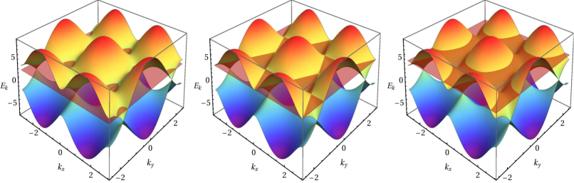
Figure 2: Band structure of tight-binding model, with Fermi-energy below (left), exactly crossing (middle) and above (right) the $M$-points (saddle points). Topology of the intersecting lines (“Fermi surface”) are different in each case.

To date, little is known about the effect of two-body interactions on the Lifshitz transition. Our goal is to clarify this issue through Monte-Carlo simulation. In particular, it will be interesting to see how a small interaction term affects the logarithmic scaling behavior. Adding a chemical potential leads to a Fermion sign-problem however, since the Fermion operators are modified as

$$M_{(x,t)(y,t^{\prime})}\to M_{(x,t)(y,t^{\prime})}+\mu\frac{\beta}{N_{t}}\delta_{xy}\delta_{t-1,t^{\prime}}~{},\quad\quad M^{\dagger}_{(x,t)(y,t^{\prime})}\to M^{\dagger}_{(x,t)(y,t^{\prime})}-\mu\frac{\beta}{N_{t}}\delta_{xy}\delta_{t+1,t^{\prime}}~{},$$ (8)

which implies that the phases in Eq. (3) no longer cancel. As a first step it is reasonable to consider an isospin chemical potential $\mu_{S}\equiv s\mu$ (the sign of $\mu_{S}$ depends on the direction of electron spin). In the non-interacting limit it is clear that the Lifshitz transition is blind to the sign of the spin. For $\mu_{S}$ there is no sign-problem since positive terms are added to both $M$ and $M^{\dagger}$.

We have so-far obtained preliminary results concerning the particle-number-susceptibility associated with $\mu_{S}$

$$\chi(\mu_{S})=\frac{1}{V\beta}\frac{d^{2}\ln{Z}}{d\mu_{S}^{2}}~{},$$ (9)

which is related to the density of states $\rho(\mu)$ (for $T=0$ they are exactly proportional) and displays the characteristic scaling behavior of the Lifshitz transition. Hereby we restricted ourselves to the the non-interacting limit, where $\chi(\mu_{S})$ can be computed directly from inversions of the Fermion matrix on Gaussian noise vectors and no HMC updates are necessary (since the Hubbard field is taken to zero). Furthermore, $\chi(\mu_{S})$ can in fact be computed exactly in this limit (by numerical integration) from the retarded particle-hole polarization (Lindhard) function (see Ref. [9]). For a given temperature $T$ it is (in infinite volume) given by

$$\chi(\mu_{S})=\frac{1}{2T}\int_{BZ}\frac{d^{2}k}{4\pi^{2}}\Big{[}\text{sech}^{2}\Big{(}\frac{\mu_{S}-E(\vec{k})}{2T}\Big{)}+\text{sech}^{2}\Big{(}\frac{\mu_{S}+E(\vec{k})}{2T}\Big{)}\Big{]}~{},$$ (10)

where $E(\vec{k})$ is the dispersion-relation of the tight-binding theory and the integral runs over the first Brillouin zone. These results are important, since they allow us to compare lattice results to direct calculations and serve as a validation of our method. Simulations at non-zero coupling are currently in progress.

Fig. 3 shows the susceptibility for two different temperatures ($\beta=2;\,4\,\mathrm{eV}^{-1}$) obtained from a $N_{x}=N_{y}=24$ lattice with $m_{s}=0.5\mathrm{eV}$. We obtained data for different lattice-spacings and extrapolated to the limit $\delta\to 0$. The results are compared to solutions of Eq. (10) (for finite volumes the integral is replaced by a sum over discrete momenta). We find exact agreement within errors. Furthermore, we have confirmed that the peak-height scales logarithmically with temperature as Eq. (10) also predicts.

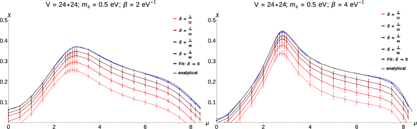
Figure 3: $\chi(\mu_{S})$ in the non-interacting limit for $N_{x}=N_{y}=24$ and $m_{s}=0.5\mathrm{eV}$. Results are obtained with different discretizations and the limit $\delta\to 0$ is extrapolated. Two temperatures ($\beta=2;\,4\,\mathrm{eV}^{-1}$) are displayed. The solid line represents the exact results, obtained from Eq. (10).

Acknowledgments

We have benefited from discussions with Pavel Buividovich, Maxim Ulybyshev and David Scheffler. This work was supported by the Deutsche Forschungsgemeinschaft within SFB 634, by the Helmholtz International Center for FAIR within the LOEWE initiative of the State of Hesse, and the European Commission, FP-7-PEOPLE-2009-RG, No. 249203. All results were obtained using Nvidia GTX and Tesla graphics cards.

References

- [1] A. H. Castro Neto et al., Rev. Mod. Phys. 81, 109 (2009); V. N. Kotov et al., Rev. Mod. Phys. 84, 1067 (2012) [arXiv:1012.3484].
- [2] V. P. Gusynin et al., Int. J. Mod. Phys. B 21 (2007) 4611 [arXiv:0706.3016].
- [3] J. E. Drut and T. A. Lähde, Phys. Rev. Lett. 102, 026802 (2009) [arXiv:0807.0834]; Phys. Rev. B 79, 165425 (2009) [arXiv:0901.0584]. W. Armour, S. Hands and C. Strouthos, Phys. Rev. B 81, 125105 (2010) [arXiv:0910.5646].
- [4] R. Brower, C. Rebbi and D. Schaich, PoS LATTICE 2011, 056 (2012) [arXiv:1204.5424]; [arXiv:1101.5131].
- [5] P. V. Buividovich and M. I. Polikarpov, Phys. Rev. B 86, 245117 (2012) [arXiv:1206.0619].
- [6] M. V. Ulybyshev, P. V. Buividovich, M. I. Katsnelson and M. I. Polikarpov, Phys. Rev. Lett. 111, 056801 (2013) [arXiv:1304.3660].
- [7] D. Smith and L. von Smekal, PoS (LATTICE 2013) 048 [arXiv:1311.1130].
- [8] D. Smith and L. von Smekal, Phys. Rev. B 89, 195429 (2014) [arXiv:1403.3620 [hep-lat]].
- [9] B. Dietz, F. Iachello, M. Miski-Oglu, N. Pietralla, A. Richter, L. von Smekal, and J. Wambach, Phys. Rev. B 88, 104101 (2013) [arXiv:1304.4764].
- [10] D. C. Elias et al., Nature Phys. 7, 701 (2011) [arXiv:1104.1396]; A. S. Mayorov et al., Nano Lett. 12, 4629 (2012), [arXiv:1206.3848].
- [11] T. O. Wehling et. al., Phys. Rev. Lett. 106, 236805 (2011) [arXiv:1101.4007].